Physics-informed Neural Network for Acoustic Resonance Analysis

Abstract

This study proposes the physics-informed neural network (PINN) framework to solve the wave equation for acoustic resonance analysis. ResoNet, the analytical model proposed in this study, minimizes the loss function for periodic solutions, in addition to conventional PINN loss functions, thereby effectively using the function approximation capability of neural networks, while performing resonance analysis. Additionally, it can be easily applied to inverse problems. Herein, the resonance in a one-dimensional acoustic tube was analyzed. The effectiveness of the proposed method was validated through the forward and inverse analyses of the wave equation with energy-loss terms. In the forward analysis, the applicability of PINN to the resonance problem was evaluated by comparison with the finite-difference method. The inverse analysis, which included the identification of the energy loss term in the wave equation and design optimization of the acoustic tube, was performed with good accuracy.

[The following article has been submitted to the Journal of the Acoustical Society of America. After it is published, it will be found at https://pubs.aip.org/asa/jasa.]

I Introduction

Machine learning has made significant advances over the last decade, yielding state-of-the-art methods in numerous fields including speech synthesis[1][2] and image recognition[3][4]. Advances in machine learning have enhanced numerical simulation technology, which has been applied to turbulence models[5][6], design optimization of machine materials[7], and to accelerate the computation time in fluid analysis[8][9]. Recent years have seen an increased demand for machine learning in numerical simulation as it effectively addresses inverse problems such as design optimization and parameter identification. The physics-informed neural network (PINN), proposed by Raissi et al. [10], is a numerical analysis method that introduces constraints on the governing partial differential equations (PDEs) in the loss functions of a neural network. In PINN, a loss function based on PDE residuals evaluated by automatic differentiation (AD)[11] along with the loss functions of the initial and boundary conditions are defined and then minimized to obtain the simulation results. The PINN can be used for inverse problems to identify uncertain parameters of the governing PDEs. It has also been applied in thermodynamics and fluid mechanics for parameter identification of the equation of state[12], application to inverse problems in supersonic flows[13], and identification of the thermal diffusivity of materials[14].

Despite the aforementioned advances in PINN, their application in the field of acoustics has been limited. Moreover, although the wave equation governing the acoustic phenomena is linear, it is subject to reflection, interference, and diffraction, and its solutions have a wide range of amplitudes and frequencies[15]. Therefore, the dynamics of sound waves can be extremely complex, thus rendering the development of PINN for acoustic analysis difficult [16]. Only a few studies have analyzed acoustic resonance using PINN.

Existing studies that employed PINN for wave equation analyses[16][17][18] have considered only unidirectional traveling waves or a small number of acoustic wave reflections and interferences, and thus, they do not apply to resonance phenomena. Several practical PINN based on the wave equation have been reported for seismic wave analysis[19][20][21]; however, they are for large-scale Earth’s ground and inapplicable to sound fields with complex dynamics, such as those of human-scale acoustic instruments. A previous study on acoustic holography using PINN based on the Kirchhoff–Helmholtz integral[22][23] demonstrated the applicability of PINN to acoustic resonance; however, this resonance analysis was in the frequency domain and could not perform time-dependent analysis.

Time-domain analysis of resonance is extremely important in the field of acoustics. For example, the two-mass model[24][25] and body-cover model[26][27] describing vocal fold vibrations in speech production, describe vocal fold vibrations as equations in the time domain. The equations describing lip motion in brass instruments[28][29] and reed motion in woodwinds[30][31] are also described as time-domain equations. Time-domain analysis of resonance using PINN could considerably benefit various acoustics fields, including the analysis of speech production and design optimization of acoustic equipment.

In this study, we propose ResoNet, a PINN that analyzes acoustic resonance in the time domain based on the wave equation while effectively utilizing the function approximation capability of neural networks[32] by training the neural network to minimize the loss function with respect to periodic solutions. The main contributions of this study are as follows. (i) This study proposes a novel framework for analyzing resonances in the time domain using PINN; (ii) it presents a detailed investigation of the applicability of PINN to acoustic resonance analysis, and (iii) it presents an investigation of the performance of inverse problem analysis on acoustic resonance phenomena.

The remainder of this paper is organized as follows. Section II describes the one-dimensional wave equation with energy loss terms, and the acoustic field setup analyzed in this study. Section III describes ResoNet, which is a PINN that analyzes resonances based on the wave equation described in Section II. Section IV describes the forward and inverse analyses using ResoNet and its performance. Section V summarizes the study and discusses the application potential of PINN in acoustic resonance.

II Governing equations of acoustic resonance

This section describes the wave equation and the acoustic field setup analyzed in this study.

II.1 One-dimensional wave equation with energy loss terms

We considered the propagation of plane sound waves in an acoustic tube of length $l$ and circular cross-sectional area of $A(x)$, as shown in Fig. 1, with $x$ as the axial direction. Let the sound pressure in the acoustic tube be $p$ and air volume velocity be $u$. Assuming $p=Pe^{j\omega t}$ and $u=Ue^{j\omega t}$, the telegrapher’s equations for the acoustic tube considering energy loss are as follows[33].

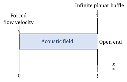
Figure 1: (Color online) Acoustic tube.

$$\dfrac{dU}{dx} =-\left(G+j\omega\dfrac{A}{K}\right)P,$$ (1)

$$\dfrac{dP}{dx} =-\left(R+j\omega\dfrac{\rho}{A}\right)U,$$ (2)

where $G$ is the coefficient of energy loss owing to thermal conduction at the tube wall; $R$ is the coefficient of energy loss owing to viscous friction at the tube wall; $j$ is the imaginary unit; $\omega$ is the angular velocity; $K$ is the bulk modulus; and $\rho$ is the air density. Equations (1) and (2) can be expressed in the time domain, as follows.

$$\dfrac{\partial u}{\partial x} =-Gp-\dfrac{A}{K}\dfrac{\partial p}{\partial t},$$ (3)

$$\dfrac{\partial p}{\partial x} =-Ru-\dfrac{\rho}{A}\dfrac{\partial u}{\partial t}.$$ (4)

The velocity potential $\phi$ is defined as:

$$u =-A\dfrac{\partial\phi}{\partial x},$$ (5)

$$p =RA\phi+\rho\dfrac{\partial\phi}{\partial t}.$$ (6)

From equations (3)-(6), we obtain the following wave equation with energy loss terms, as follows.

$$\dfrac{\partial^{2}\phi}{\partial x^{2}}+\dfrac{1}{A}\dfrac{\partial A}{\partial x}\dfrac{\partial\phi}{\partial x}=GR\phi+\left(\dfrac{G\rho}{A}+\dfrac{RA}{K}\right)\dfrac{\partial\phi}{\partial t}+\dfrac{\rho}{K}\dfrac{\partial^{2}\phi}{\partial t^{2}}.$$ (7)

Detailed derivation of Eq. (7) is provided in Appendix A.

Theoretical solutions for $R$ and $G$ have been proposed, as follows, under the assumptions that the wall surface is rigid and thermal conductivity is infinite[33].

$$R =\dfrac{S}{A^{2}}\sqrt{\dfrac{\omega_{c}\rho\mu}{2}},$$ (8)

$$G =S\dfrac{\eta-1}{\rho c^{2}}\sqrt{\dfrac{\lambda\omega_{c}}{2c_{p}\rho}},$$ (9)

where $S$ is the circumference of the acoustic tube; $\mu$, $\eta$, $c$, $\lambda$, and $c_{p}$ are the viscosity coefficient, heat-capacity ratio, speed of sound, thermal conductivity, and specific heat at constant pressure, respectively; and $\omega_{c}$ is the angular velocity used to calculate the energy loss term. As $R$ and $G$ vary with the physical properties of air and the condition of the walls of the acoustic tube, these parameters are generally unknown. We confirmed that the energy loss parameters of the acoustic tube should be measured experimentally[34]. Additionally, as demonstrated in the field of vocal tract analysis, we have experimentally confirmed that the energy loss parameters can be approximated as frequency-independent constants in a limited frequency range[34]. Therefore, in this study, $\omega_{c}$ was set as constant, and consequently, $R$ and $G$ were assumed to be frequency-independent constants.

II.2 Acoustic field and boundary conditions

The acoustic field analyzed in this study is shown in light blue in Fig. 1. The acoustic tube was straight, and a forced-flow boundary condition was given at $x=0$. It had an open end with an infinite planar baffle at $x=l$, and the boundary condition was given by the equivalent circuit described in Section II.3.

The above boundary conditions are fundamental in human speech production[24][25] and in the acoustic analysis of brass instruments[35]. In this study, we used these boundary conditions to investigate the performance of resonance analysis with PINN.

II.3 Modeling of radiation

This section describes the modeling of the radiation at $x=l$ in Fig. 1. Assuming that the particle velocity $u_{l}$ at the open end is uniform, air at the open end can be regarded as a planar sound source. In response to the acoustic radiation, the plane receives sound pressure $p_{l}$ from outside the acoustic tube. If the open end is surrounded by an infinite planar baffle, the relationship between $u_{l}$ and $p_{l}$ can be approximated using the equivalent circuit shown in Fig. 2[24]. In Fig. 2, the volume velocity $u_{l}$ corresponds to the current and the sound pressure $p_{l}$ to the voltage. The equations connecting $u_{l}$ and $p_{l}$ are as follows.

$$\left(u_{l}-u_{r}\right)R_{r} =L_{r}\dfrac{du_{r}}{dt},$$ (10)

$$p_{l} =\left(u_{l}-u_{r}\right)R_{r},$$ (11)

where $R_{r}$ is the circuit resistance; $L_{r}$ is the circuit reactance; and $u_{l}$ is the current (corresponding to the volume velocity) flowing through the coil side. Here, $R_{r}$ and $L_{r}$ are expressed as follows.

$$R_{r} =\dfrac{128\rho c}{9\pi^{2}A_{r}},$$ (12)

$$L_{r} =\dfrac{8\rho}{3\pi\sqrt{\pi A_{r}}},$$ (13)

where $A_{l}$ denotes the cross-sectional area for $x=l$.

Figure 2: Equivalent circuit of acoustic radiation.

III Proposed method

This section describes the structure of ResoNet, a PINN for analyzing the acoustic resonance, and a training method for the neural network.

III.1 Overview of ResoNet

The proposed neural network structure for the resonance analysis in acoustic tubes is shown in Fig. 3; we refer to this architecture as ResoNet. As shown in Fig. 3, ResoNet has two blocks of neural networks.

The first is a network that calculates the solutions to the wave equation in Eq. (7), taking $x_{i}$ and $t_{i}$ as inputs (where $i$ is the sample number) to predict the velocity potential $\hat{\phi}_{i}$. In this study, this input–output relationship is expressed in the following equation.

$$\hat{\phi}_{i}=F_{w}\left(x_{i},t_{i};\Theta_{w}\right),$$ (14)

where $F_{w}$ is the operator of the neural network for the wave equation and $\Theta_{w}$ is the set of trainable parameters of the neural network.

The other is a network for calculating the acoustic radiation, utilizing $t_{i}$ as the input for predicting $\hat{u}_{ri}$ by calculating the solution of the equivalent circuit in Fig. 2. The input–output relationship is expressed as:

$$\hat{u}_{ri}=F_{r}\left(t_{i};\Theta_{r}\right),$$ (15)

where $F_{r}$ is the operator of the neural network for acoustic radiation analysis and $\Theta_{r}$ is the set of trainable parameters of the neural network.

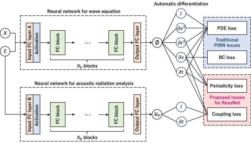
Figure 3: (Color online) Structure of ResoNet.

Automatic differentiation is performed on $\hat{\phi}_{i}$ and $\hat{u}_{ri}$, and the various loss functions shown on the right side of Fig. 3 are defined. The traditional PINN uses the PDE and boundary condition (BC) loss functions. The PDE loss introduces the constraints of Eq. (7), and the BC loss introduces constraints owing to the boundary conditions into the neural network. We used periodicity loss and coupling loss as the loss functions for ResoNet, where periodicity loss introduced constraints owing to the resonance periodicity, and coupling loss introduced constraints owing to the coupling of the wave equation and the external system (acoustic radiation in this study) into the neural network. Each item is described in detail in the following sections.

III.2 Neural network blocks

As shown in Fig. 3, ResoNet has two neural network blocks: one calculates the solution of the wave equation in Eq. (7), whereas the other calculates the solution for the acoustic radiation circuit in Fig. 2.

III.2.1 Neural network for wave equation

This network uses $x_{i}$ and $t_{i}$ as inputs, and predicts the velocity potential $\hat{\phi}_{i}$ for the wave equation. Initially, two-channel data ($x_{i}$, $t_{i}$) are fed to ”Input FC layer A” which is a fully connected layer[36] that outputs $N_{f}$ channel data as shown in Fig. 3. An activation layer is present immediately afterward, and it is given by:

$$f(a)=a+\sin^{2}a,$$ (16)

where $a$ denotes the input to layer. This activation function is called a Snake, and has been reported to be robust to periodic inputs[37].

After the first activation layer, data is fed into the ”FC block.” All FC blocks in Fig. 3 have the same structure, and its details are shown in Fig. 4. The fully connected layer in Fig. 4 has $N_{f}$ input channels and $N_{f}$ output channels, and the activation layer is the Snake, as shown in Eq. (16). To circumvent the vanishing gradient problem[38], a residual connection[39] is applied before the last activation layer.

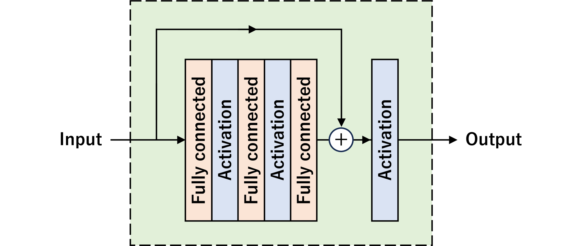
Figure 4: (Color online) Details of FC block.

After $N_{b}$ FC blocks, the data is fed into the ”Output FC layer” which is a fully connected layer with $N_{f}$ input channels and one output channel that predicts the $\hat{\phi}_{i}$ value of the solution for the wave equation.

III.2.2 Neural network for acoustic radiation analysis

This network uses $t_{i}$ as the input, and predicts the $\hat{u}_{ri}$ value of the equivalent circuit shown in Fig. 2. The only difference from the neural network for the wave equation (described in Section III.2.1) is that the number of input channels is one ($t_{i}$ only) and the ”Input FC layer B” is a fully connected layer with one input channel and $N_{f}$ output channels. All the other structures are identical to those described in Section III.2.1.

III.3 Loss functions

The loss function of ResoNet is calculated as the sum of the following partial loss functions: traditional PINN losses (PDE loss and BC loss), periodicity loss, and coupling loss.

III.3.1 Traditional PINN losses

For PDE loss, the output $\hat{\phi}_{i}$ of the neural network is defined as:

$$\hat{\phi}_{i,E}:=F_{w}\left(x_{i},t_{i};\Theta_{w}\right),\quad x_{i}\in\left[0,l\right],\quad t_{i}\in\left[0,T\right],$$ (17)

where $T$ is the simulation time ( one resonance period in this study). For $\hat{\phi}_{i,E}$ to follow Eq. (7), the PDE loss is defined as:

$$\begin{split}L_{E}&=\dfrac{1}{N_{E}}\sum_{i=1}^{N_{E}}\left\{\dfrac{\partial^{2}\hat{\phi}_{i,E}}{\partial x_{i}^{2}}+\dfrac{1}{A_{i}}\dfrac{\partial A_{i}}{\partial x_{i}}\dfrac{\partial\hat{\phi}_{i,E}}{\partial x_{i}}-G_{i}R_{i}\hat{\phi}_{i,E}\right.\\ &\left.\quad-\left(\dfrac{G_{i}\rho}{A_{i}}+\dfrac{R_{i}A_{i}}{K}\right)\dfrac{\partial\hat{\phi}_{i,E}}{\partial t_{i}}-\dfrac{\rho}{K}\dfrac{\partial^{2}\hat{\phi}_{i,E}}{\partial t_{i}^{2}}\right\}^{2},\end{split}$$ (18)

where $N_{E}$ is the number of collocation points for the PDE loss. The partial differential values of $\hat{\phi}_{i,E}$ required to calculate Eqs. (18) are obtained via automatic differentiation[38] of the neural network.

Similarly, $\hat{\phi}_{i}$ must follow boundary conditions. As described in Section II.2, the boundary condition in this study at $x=0$ is given by the forced flow velocity. For the BC loss, the output $\hat{\phi}_{i}$ of the neural network is defined as:

$$\hat{\phi}_{i,B}:=F_{w}\left(x_{0},t_{i};\Theta_{w}\right),\quad t_{i}\in\left[0,T\right],$$ (19)

where $x_{0}=0$. The loss function $L_{B}$ with respect to the boundary condition is defined as:

$$L_{B}=\dfrac{1}{N_{B}}\sum_{i=1}^{N_{B}}\left(\hat{u}_{i,B}-\bar{u}_{i,B}\right)^{2},$$ (20)

where $N_{B}$ is the number of collocation points for the BC loss and $\bar{u}_{i,B}$ is the volume flow velocity data given as the boundary condition. Based on Eq. (5), $\hat{u}_{i,B}$ is calculated from $\hat{\phi}_{i,B}$ using the following equation.

$$\hat{u}_{i}=-A_{i}\dfrac{\partial\hat{\phi}_{i}}{\partial x_{i}}.$$ (21)

III.3.2 Periodicity loss

This section explains the core idea of ResoNet, the loss function with respect to periodicity. When performing time-domain resonance analysis, the transient state must be included until a steady state is reached. As mentioned in Section I, because sound waves have complex dynamics, a large-scale neural network is required to perform long simulations, which poses challenges in terms of the computational cost and neural network convergence.

In the acoustic resonance analysis, the object of interest is one period in the steady state, as shown in Fig. 5. Therefore, in ResoNet, only one period was analyzed and the function approximation capability of the neural network was effectively used. For this purpose, we proposed a ”periodicity loss,” which forces the output of the neural network to have the same value as $\hat{\phi}_{i}$ at $t=0$ and $t=T$ in the steady state. The following describes the procedure for calculating periodicity loss.

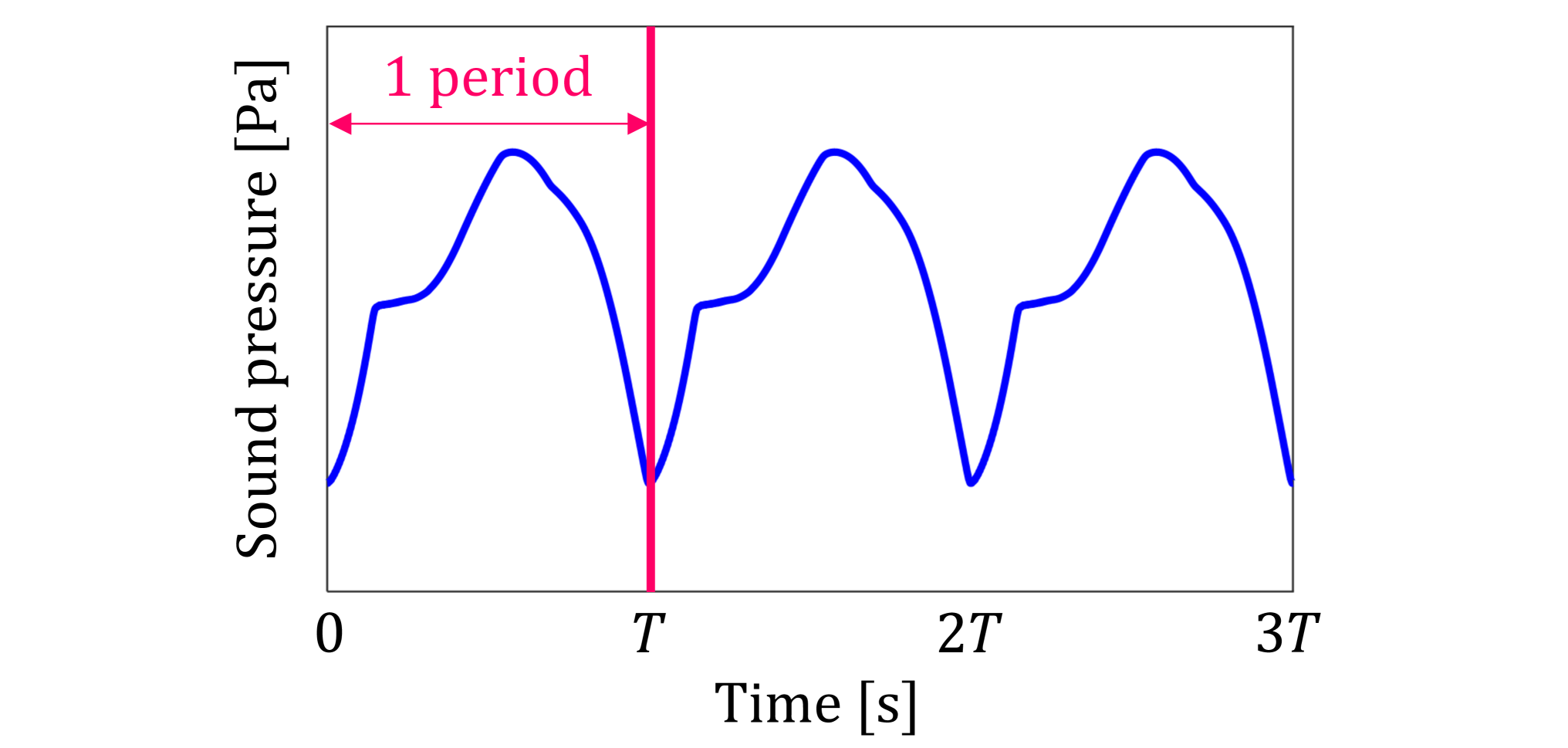
Figure 5: (Color online) Sound pressure waveform at steady state of resonance.

First, the output $\hat{\phi}_{i}$ of the neural network for the wave equation is defined using the following two equations.

$$\begin{array}[]{c}\hat{\phi}_{i,P1}:=F_{w}\left(x_{i},t_{0};\Theta_{w}\right)\\ \hat{\phi}_{i,P2}:=F_{w}\left(x_{i},t_{T};\Theta_{w}\right)\end{array},\quad x_{i}\in\left[0,l\right],$$ (22)

where $t_{0}=0$ and $t_{T}=T$ ($T$: period); and $\phi_{i,P1}$ and $\phi_{i,P2}$ are the values of the output $\hat{\phi}_{i}$ for times $t=0$ and $t=T$ at the same position $x_{i}$, respectively.

Based on Eq. (6), the sound pressure is obtained from $\hat{\phi}_{i}$ as follows.

$$\hat{p}_{i}=R_{i}A_{i}\hat{\phi}_{i}+\rho\dfrac{\partial\hat{\phi}_{i}}{\partial t_{i}}.$$ (23)

The volume velocity is obtained from $\hat{\phi}_{i}$ using Eq. (21). Let $\hat{u}_{i,P1}$ and $\hat{p}_{i,P1}$ be the volume velocity and sound pressure obtained from $\hat{\phi}_{i,P1}$, and let $\hat{u}_{i,P2}$ and $\hat{p}_{i,P2}$ be those obtained from $\hat{\phi}_{i,P2}$, respectively. In the steady state, if the input $x_{i}$ (position) is the same, the continuity condition must hold between $\hat{p}_{i,P1}$ and $\hat{p}_{i,P2}$ and between $\hat{u}_{i,P1}$ and $\hat{u}_{i,P2}$. Therefore, the following loss functions are defined to force the neural network to enforce the conditions $\hat{p}_{i,P1}=\hat{p}_{i,P2}$ and $\hat{u}_{i,P1}=\hat{u}_{i,P2}$.

$$L_{u} =\dfrac{1}{N_{P}}\sum_{i=1}^{N_{P}}\left(\hat{u}_{i,P1}-\hat{u}_{i,P2}\right)^{2}$$ (24)

$$L_{p} =\dfrac{1}{N_{P}}\sum_{i=1}^{N_{P}}\left(\hat{p}_{i,P1}-\hat{p}_{i,P2}\right)^{2},$$ (25)

where $N_{P}$ is the number of collocation points for the periodicity loss. Additionally, we define the following loss function to enforce the continuous condition of the time derivative.

$$L_{t}=\dfrac{1}{N_{P}}\sum_{i=1}^{N_{P}}\left(\dfrac{\partial^{2}\hat{\phi}_{i,P1}}{\partial t_{0}^{2}}-\dfrac{\partial^{2}\hat{\phi}_{i,P2}}{\partial t_{T}^{2}}\right)^{2}.$$ (26)

From Eqs. (24)–(26), the periodicity loss $L_{P}$ proposed in this study is defined as

$$L_{P}=\lambda_{u}L_{u}+\lambda_{p}L_{p}+\lambda_{t}L_{t},$$ (27)

where $\lambda_{u}$, $\lambda_{p}$ and $\lambda_{t}$ are the weight parameters for each term.

III.3.3 Coupling loss

In ResoNet, the coupling condition between the system described by the wave equation and external system is introduced as the coupling loss. In this study, the external system is an acoustic radiation system, as shown in Fig. 2, and the Eqs. (10) and (11) describe coupling. In this section, we describe a method for calculating the coupling loss.

First, we define the output $\hat{\phi}_{i}$ of the neural network for the wave equation as:

$$\hat{\phi}_{i,C}:=F_{w}\left(x_{l},t_{i};\Theta_{w}\right),\quad\quad t_{i}\in\left[0,T\right],$$ (28)

where $x_{l}=l$. Let $\hat{u}_{i,C}$ and $\hat{p}_{i,C}$ be the volume velocity and sound pressure at $x=l$, obtained by applying Eqs. (21) and (23) to $\hat{\phi}_{i,C}$, respectively. Additionally, as defined in Eq. (15), let $\hat{u}_{ri}$ be the output of the neural network for acoustic radiation for input $t_{i}$. Based on Eqs. (10) and (11), the coupling loss $L_{C}$ is defined as:

$$\begin{split}L_{C}&=\dfrac{\lambda_{l}}{N_{C}}\sum_{i=1}^{N_{C}}\left\{\left(\hat{u}_{ri}-\hat{u}_{i,C}\right)R_{r}-L_{r}\dfrac{d\hat{u}_{ri}}{dt_{i}}\right\}^{2}\\ &\quad+\dfrac{\lambda_{r}}{N_{C}}\sum_{i=1}^{N_{C}}\left\{\hat{p}_{i,C}-\left(\hat{u}_{ri}-\hat{u}_{i,C}\right)R_{r}\right\}^{2},\end{split}$$ (29)

where $N_{C}$ is the number of collocation points of the coupling loss; and $\lambda_{l}$ and $\lambda_{r}$ are the weight parameters of each term.

III.3.4 Loss function for the whole network

The loss function $L_{all}$ for the entire network was calculated as the sum of the traditional PINN losses, periodic loss, and coupling loss, as follows.

$$L_{all}=\lambda_{E}L_{E}+\lambda_{B}L_{B}+\lambda_{P}L_{P}+\lambda_{C}L_{C},$$ (30)

where $\lambda_{E}$, $\lambda_{B}$, $\lambda_{P}$, and $\lambda_{C}$ denote the weight parameters of the respective loss functions. Finally, the optimization problem of ResoNet was formulated as:

$$\min_{\Theta_{w},\Theta_{r}}L_{all}(\Theta_{w},\Theta_{r}).$$ (31)

By minimizing the loss function $L_{all}$, the trainable parameters $\Theta_{w}$ and $\Theta_{r}$ of the neural network were optimized. For this purpose, we used the Adam optimizer[40] to determine the optimal values of $\Theta_{w}$ and $\Theta_{r}$ through iterative calculations.

III.4 Implementation

We implemented ResoNet using the Deep Learning Toolbox in MATLAB (MathWorks, USA) and used the ”dlfeval” function to code a custom training loop. We used ”sobolset” function from the Statistics and Machine Learning Toolbox to create datasets for $x_{i}$ and $t_{i}$. The neural network was trained via GPU-assisted computation using the Parallel Computing Toolbox.

The neural network training and prediction were performed on a computer equipped with a Core i9-13900KS CPU (Intel, USA) and GeForce RTX 4090 GPU (NVIDIA, USA) with 128 GB of main memory and 24 GB of video memory.

IV Validation of proposed method

The performance of the proposed method was validated through forward and inverse analysis of the acoustic resonance using ResoNet.

IV.1 Forward analysis

IV.1.1 Analysis conditions for forward analysis

The effectiveness of the proposed method was assessed through a forward analysis of the acoustic tube, as shown in Fig. 1 using the boundary conditions described in Section II.2. The length of the acoustic tube, $l$, was set to 1 m, and the diameter was set to 10 mm.

Note that the forced-flow velocity waveform, given as a boundary condition, is a smoothed Rosenberg wave[41] as shown in Fig. 6. To smooth the waveform, similar to an R++ wave[42], a moving average filter was applied to the original Rosenberg wave. The fundamental frequency $F_{0}$ of the forced flow waveform was 261.6 Hz (C4 on the musical scale). Therefore, $T=3.82\times 10^{-3}$ s.

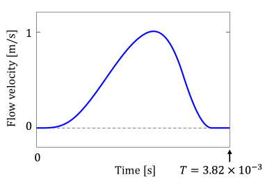
Figure 6: (Color online) Forced flow velocity waveform (smoothed Rosenberg waveform).

The physical properties of air used in the analysis are listed in Table 1. For the energy loss coefficients, Ishizaka et al. calculated $R$ by substituting a constant for $\omega_{c}$ in Eqs. (8)[24]. In this study, we calculated $R$ and $G$ by substituting $\omega_{c}=1643.7$ rad/s (261.6 Hz, C4 in the musical scale) in Eqs. (8) and (9), respectively; thus, we obtained $R=6.99\times 10^{5}$ $\mathrm{m^{2}/(Pa\cdot s)}$ and $G=3.65\times 10^{-7}$ $\mathrm{Pa\cdot s/m^{4}}$.

Table 1: Physical properties of air.

Parameter	Value
Air density $\rho$	1.20 $\mathrm{kg/m^{3}}$
Bulk modulus $K$	$1.39\times 10^{5}$ $\mathrm{Pa}$
Speed of sound $c$	340 $\mathrm{m/s}$
Viscosity coefficient $\mu$	19.0$\times 10^{-6}$ $\mathrm{Pa\cdot s}$
Heat capacity ratio $\eta$	1.40
Thermal conductivity $\lambda$	2.41$\times 10^{-2}$ $\mathrm{W/(m\cdot K)}$
Specific heat for const. pressure $c_{p}$	1.01 $\mathrm{kJ/(kg\cdot K)}$

In the forward analysis, the number of nodes in the neural network $N_{f}$ was set to 200 and the number of FC blocks $N_{b}$ was set to five. Further, a dataset ($x_{i}$, $t_{i}$) for each loss function was created, as follows. In Eq. (17) for the PDE loss calculation, we used quasi-random numbers generated by the ”sobolset” function in MATLAB for $x_{i}$ and $t_{i}$, and the number of collocation points $N_{E}$ was 5000. Next, for $t_{i}$ in Eq. (19), and Eq. (28) used in the calculation of the BC and coupling losses, the range $[0,T]$ was divided into 1000 equal parts to create a dataset of $t_{i}$; thus, $N_{B}$ and $N_{C}$ were 1000. Finally, for $x_{i}$ in Eqs. (22) used in the calculation of the periodicity loss, the range $[0,l]$ was divided into 1000 equal parts to create a dataset of $x_{i}$; thus, $N_{P}$ was 1000. As in Rasht-Behesht et al.[20], the value ranges of $x_{i}$ and $t_{i}$ were normalized to $[-1,1]$ when inputting them into the neural network.

IV.1.2 Results of forward analysis

Figure 7(a) shows the analyzed sound pressure in the range of $x=[0,l]$ and $t=[0,T]$ after 20,000 training epochs. Although only one period was analyzed, the same result is shown twice along the time axis to confirm the continuity of the waveform at $t=0$ and $t=T$. The results of the finite difference method (FDM) is shown for comparison in Fig. 7(b). Figure 7 demonstrates strong agreement between the ResoNet and FDM analysis results. Figure 8 shows the differences between the results of ResoNet and FDM. The difference was less than 1% in most regions; however, some streaked regions with a difference of 2% or more were noted. The regions with large differences are discussed later in this section.

Fig7a.pdf8cm(a) Result of ResoNet. Fig7b.pdf8cm(b) Result of FDM.

Figure 7: (Color online) Analyzed sound pressure.

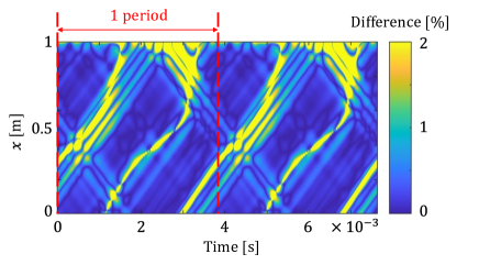
Figure 8: (Color online) Error of the ResoNet from the FDM.

Figure 9 shows the analyzed sound pressure waveforms at $x=l$ and Fig. 10 shows the frequency spectra. Although differences are observed in the high-frequency domain in Fig. 10, the ResoNet results in the time domain indicate its high accuracy in acoustic resonance analysis.

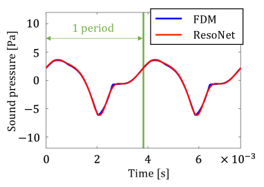
Figure 9: (Color online) Sound pressure waveforms at $x=l$.

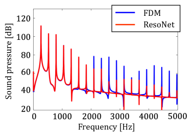
Figure 10: (Color online) Frequency spectra of the waveforms of Fig. 9.

The regions with large differences in Fig. 8 were discussed considering the sound pressure waveform and frequency spectra. Figure 11 shows the difference and sound pressure waveforms for one period on the same timescale; evidently, the difference is particularly large in region A. The corresponding region in the sound pressure waveform shows a difference between the FDM and ResoNet waveforms at the points indicated by B and C. At point B, the waveform suddenly changes from monotonically decreasing to monotonically increasing, and at point C, it shifts from monotonically increasing to a horizontal phase. Considering that a neural network is a function approximator, such steep waveform changes may not have been approximated well by ResoNet. This is evident from the difference between FDM and ResoNet in the high-frequency region shown in Fig. 10. Thus, similar to other PINNs, ResoNet accurately analyzes in the low-frequency domain; however, its accuracy degrades in the high-frequency domain. This could be improved by modifying the structure of the neural network and learning method, and this remains a subject for future studies.

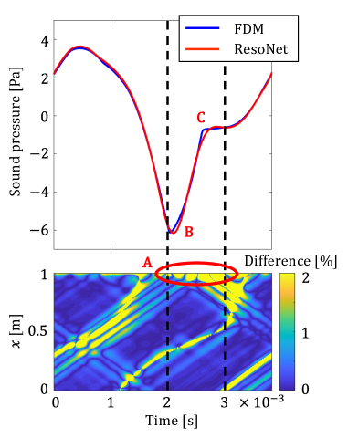
Figure 11: (Color online) Sound pressure waveforms at $x=l$ and errors in the same time scale.

The training time was 5267 s; however, the trained ResoNet could run a simulation in 0.86 s, which is approximately four times faster than FDM’s 3.67 s. Additionally, because ResoNet is a PINN-based method, it allows meshless analysis.

IV.2 Inverse analysis

Additionally, we performed an inverse analysis on the acoustic tube, as shown in Fig. 1, using the boundary conditions in Section II.2. The forced-flow waveform and physical properties were identical to those described in Section IV.1.1.

We considered two specific situations for inverse analysis: first, the identification of energy loss coefficients, and second, the design optimization of acoustic tubes. The information provided to ResoNet has two waveforms: a flow waveform at $x=0$ and a sound pressure waveform at $x=L$.

IV.2.1 Additional loss function for inverse analysis

The loss function for the sound pressure waveform at $x=l$ was introduced into ResoNet using the following procedure: First, the output $\hat{\phi}_{i,M}$ is defined as:

$$\hat{\phi}_{i,M}:=F_{w}\left(x_{l},t_{i};\Theta_{w}\right),\quad t_{i}\in\left[0,T\right],$$ (32)

where $x_{l}=l$. The loss function for the sound pressure at $x=l$ is defined as:

$$L_{M}=\dfrac{1}{N_{M}}\sum_{i=1}^{N_{M}}\left(\hat{p}_{i,M}-\bar{p}_{i,M}\right)^{2},$$ (33)

where $N_{M}$ denotes the number of collocation points for the loss. $\hat{p}_{i,M}$ was obtained from $\hat{\phi}_{i,M}$ by using Eq. (23) and $\bar{p}_{i,M}$, the measured sound pressure waveform, was obtained from the analysis results of FDM simulation. The waveform is shown in Fig. 12. The loss function for the entire network is defined as:

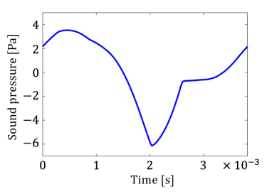
Figure 12: (Color online) Sound pressure waveform at $x=l$ (obtained by FDM simulation).

$$L_{all}=\lambda_{E}L_{E}+\lambda_{B}L_{B}+\lambda_{P}L_{P}+\lambda_{C}L_{C}+\lambda_{M}L_{M},$$ (34)

where $\lambda_{M}$ is the weight parameter of $L_{M}$.

In the inverse analysis, the number of nodes in the neural network $N_{f}$ was set to 400 and the number of FC blocks $N_{b}$ was set to two.

IV.2.2 Case 1: Identification of energy loss coefficients

Assuming that the energy-loss coefficients follow Eqs. (8)–(9) and $\omega_{c}$ in these equations is unknown, we performed an inverse analysis to determine $\omega_{c}$. As described at the beginning of section IV.2, the flow velocity waveform at $x=0$ (Fig. 6) and the sound pressure waveform at position $x=l$ (Fig. 12) are given to ResoNet. Because $w_{c}$ is a trainable parameter of the neural network, the optimization problem was formulated as:

$$\min_{\Theta_{w},\Theta_{r},\omega_{c}}L_{all}(\Theta_{w},\Theta_{r},\omega_{c}).$$ (35)

The identification results are shown in Fig. 13. The initial value of $\omega_{c}$ was set to $1.3149\times 10^{3}$ (20% error) for a true value of $1.6437\times 10^{3}$; however, after 100,000 training epochs, the value converged to $1.6671\times 10^{3}$, which indicated that $\omega_{c}$ could be identified with an error of 1.01%.

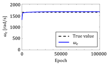
Figure 13: (Color online) Identification result of $\omega_{c}$.

IV.2.3 Case 2: Design optimization of acoustic tube

This section describes the design optimization of the length $l$ and diameter $d$ of the acoustic tube that simultaneously satisfy the flow velocity waveform at $x=0$ and the sound pressure waveform at $x=l$. The flow velocity waveform at $x=0$ in Fig. 6 and the sound pressure waveform at $x=l$ in Fig. 12 were given to ResoNet. Because $l$ and $d$ are the trainable parameters of the neural network, the optimization problem was formulated as:

$$\min_{\Theta_{w},\Theta_{r},l,d}L_{all}(\Theta_{w},\Theta_{r},l,d).$$ (36)

The identification results are shown in Fig. 14. The initial value of $l$ was set to 0.8 (20% error) for an optimal value of 1 and the initial value of $d$ was set to 8 (20% error) for an optimal value of 10. Table 2 indicates that $l$ and $d$ were identified with high accuracy with respect to the optimal values after 100,000 training epochs.

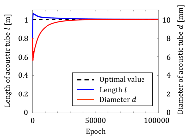
Figure 14: (Color online) Identification result of $l$ and $d$.

Table 2: Optimal and identified value of $l$ and $d$.

	Optimal	Identified
Length $l$ [m]	1	1.0022 (0.22% error)
Diameter $d$ [mm]	10	10.009 (0.09% error)

V Conclusion

In this study, we proposed ResoNet, a PINN for analyzing acoustic resonance, and demonstrated its effectiveness by performing a time-domain analysis of acoustic resonance by introducing a loss function for periodicity into a neural network.

The forward analysis performed using an acoustic tube of length 1 m, which is the scale of a musical instrument or car muffler, revealed that acoustic resonance analysis could be performed with sufficient accuracy in the time domain. The analysis accuracy decreased with abrupt changes in the sound pressure waveform and also in the high-frequency region in the frequency domain. Given that this is due to the function approximation capability of the neural network, designing a PINN structure that is more suitable for acoustic analysis is a topic for future studies. The trained ResoNet can perform simulations approximately four times faster than FDM, and as a PINN-based method, ResoNet offers the advantage of meshless analysis.

For the inverse analysis, the identification of energy loss coefficient in the acoustic tube and the design optimization of the acoustic tube were performed. In these inverse problems, the true and optimal values could be identified with high accuracy from the waveform data at the endpoints of the acoustic tube.

These results demonstrate that ResoNet enables analyzing acoustic inverse problems without requiring the advanced creation of specialized analytical models for each problem. This highlights the potential for broad applicability not only for parameter identification but also to other inverse problems related to 1D acoustic tubes, such as the design optimization of musical instruments and glottal inverse filtering (GIF). In future work, we intend to address these acoustic inverse problems using ResoNet.

Appendix A Derivation of wave equation

This section describes the derivation of the wave equation using the energy-loss terms (Eq. (7)). First, the telegrapher’s equation in the time domain (Eq. (3) and (4)).

$$\dfrac{\partial u}{\partial x} =-Gp-\dfrac{A}{K}\dfrac{\partial p}{\partial t},$$ (37)

$$\dfrac{\partial p}{\partial x} =-Ru-\dfrac{\rho}{A}\dfrac{\partial u}{\partial t}.$$ (38)

The velocity potential is defined as:

$$u =-A\dfrac{\partial\phi}{\partial x}.$$ (39)

By substituting Eq. (39) into Eq. (38), we obtain:

$$p =RA\phi+\rho\dfrac{\partial\phi}{\partial t}.$$ (40)

By substituting Eqs. (39) and (40) into Eq. (37), we obtain:

$$\begin{split}-\dfrac{\partial}{\partial x}\left(A\dfrac{\partial\phi}{\partial x}\right)&=-G\left(RA\phi+\rho\dfrac{\partial\phi}{\partial t}\right)\\ &\quad-\dfrac{A}{K}\dfrac{\partial}{\partial t}\left(RA\phi+\rho\dfrac{\partial\phi}{\partial t}\right).\end{split}$$ (41)

By expanding and simplifying Eq. (41), we obtain the following wave equation with energy loss terms.

$$\dfrac{\partial^{2}\phi}{\partial x^{2}}+\dfrac{1}{A}\dfrac{\partial A}{\partial x}\dfrac{\partial\phi}{\partial x}=GR\phi+\left(\dfrac{G\rho}{A}+\dfrac{RA}{K}\right)\dfrac{\partial\phi}{\partial t}+\dfrac{\rho}{K}\dfrac{\partial^{2}\phi}{\partial t^{2}}.$$ (42)

References

- [1] A. v. d. Oord, S. Dieleman, H. Zen, K. Simonyan, O. Vinyals, A. Graves, N. Kalchbrenner, A. Senior, and K. Kavukcuoglu, “Wavenet: A generative model for raw audio,” arXiv:1609.03499 (2016).
- [2] I. Elias, H. Zen, J. Shen, Y. Zhang, Y. Jia, R. Skerry-Ryan, and Y. Wu, “Parallel Tacotron 2: A Non-Autoregressive Neural TTS Model with Differentiable Duration Modeling,” in Proc. Interspeech 2021 (2021), pp. 141–145.
- [3] A. Krizhevsky, I. Sutskever, and G. E. Hinton, “Imagenet classification with deep convolutional neural networks,” in Advances in Neural Information Processing Systems (2012), Vol. 25.
- [4] F. N. Iandola, S. Han, M. W. Moskewicz, K. Ashraf, W. J. Dally, and K. Keutzer, “Squeezenet: Alexnet-level accuracy with 50x fewer parameters and¡ 0.5 mb model size,” arXiv:1602.07360 (2016).
- [5] J. Ling, A. Kurzawski, and J. Templeton, “Reynolds averaged turbulence modelling using deep neural networks with embedded invariance,” Journal of Fluid Mechanics 807, 155–166 (2016).
- [6] R. Fang, D. Sondak, P. Protopapas, and S. Succi, “Neural network models for the anisotropic reynolds stress tensor in turbulent channel flow,” Journal of Turbulence 21(9-10), 525–543 (2020).
- [7] K. Guo, Z. Yang, C.-H. Yu, and M. J. Buehler, “Artificial intelligence and machine learning in design of mechanical materials,” Materials Horizons 8(4), 1153–1172 (2021).
- [8] D. Kochkov, J. A. Smith, A. Alieva, Q. Wang, M. P. Brenner, and S. Hoyer, “Machine learning–accelerated computational fluid dynamics,” Proceedings of the National Academy of Sciences 118(21), e2101784118 (2021).
- [9] B. Kim, V. C. Azevedo, N. Thuerey, T. Kim, M. Gross, and B. Solenthaler, “Deep fluids: A generative network for parameterized fluid simulations,” in Computer graphics forum (2019), Vol. 38, pp. 59–70.
- [10] M. Raissi, P. Perdikaris, and G. E. Karniadakis, “Physics-informed neural networks: A deep learning framework for solving forward and inverse problems involving nonlinear partial differential equations,” Journal of Computational physics 378, 686–707 (2019).
- [11] L. B. Rall, Automatic differentiation: Techniques and applications (Springer, 1981).
- [12] Z. Mao, A. D. Jagtap, and G. E. Karniadakis, “Physics-informed neural networks for high-speed flows,” Computer Methods in Applied Mechanics and Engineering 360, 112789 (2020).
- [13] A. D. Jagtap, Z. Mao, N. Adams, and G. E. Karniadakis, “Physics-informed neural networks for inverse problems in supersonic flows,” Journal of Computational Physics 466, 111402 (2022).
- [14] S. Cai, Z. Wang, S. Wang, P. Perdikaris, and G. E. Karniadakis, “Physics-informed neural networks for heat transfer problems,” Journal of Heat Transfer 143(6), 060801 (2021).
- [15] H. Igel, Computational Seismology: A Practical Introduction (Oxford University Press, 2016).
- [16] B. Moseley, A. Markham, and T. Nissen-Meyer, “Solving the wave equation with physics-informed deep learning,” arXiv preprint arXiv:2006.11894 (2020).
- [17] S. Alkhadhr, X. Liu, and M. Almekkawy, “Modeling of the forward wave propagation using physics-informed neural networks,” in 2021 IEEE International Ultrasonics Symposium (IUS) (2021), pp. 1–4.
- [18] H. Wang, J. Li, L. Wang, L. Liang, Z. Zeng, and Y. Liu, “On acoustic fields of complex scatters based on physics-informed neural networks,” Ultrasonics 128, 106872 (2023).
- [19] S. Karimpouli and P. Tahmasebi, “Physics informed machine learning: Seismic wave equation,” Geoscience Frontiers 11(6), 1993–2001 (2020).
- [20] M. Rasht-Behesht, C. Huber, K. Shukla, and G. E. Karniadakis, “Physics-informed neural networks (pinns) for wave propagation and full waveform inversions,” Journal of Geophysical Research: Solid Earth 127(5), e2021JB023120 (2022).
- [21] Y. Zhang, X. Zhu, and J. Gao, “Seismic inversion based on acoustic wave equations using physics-informed neural network,” IEEE transactions on geoscience and remote sensing 61, 1–11 (2023).
- [22] M. Olivieri, M. Pezzoli, F. Antonacci, and A. Sarti, “A physics-informed neural network approach for nearfield acoustic holography,” Sensors 21(23), 7834 (2021).
- [23] H. Kafri, M. Olivieri, F. Antonacci, M. Moradi, A. Sarti, and S. Gannot, “Grad-cam-inspired interpretation of nearfield acoustic holography using physics-informed explainable neural network,” in ICASSP 2023-2023 IEEE International Conference on Acoustics, Speech and Signal Processing (ICASSP) (2023), pp. 1–5.
- [24] K. Ishizaka and J. L. Flanagan, “Synthesis of voiced sounds from a two-mass model of the vocal cords,” Bell system technical journal 51(6), 1233–1268 (1972).
- [25] L. Cveticanin et al., “Review on mathematical and mechanical models of the vocal cord,” Journal of Applied Mathematics 2012 (2012).
- [26] B. H. Story and I. R. Titze, “Voice simulation with a body-cover model of the vocal folds,” The Journal of the Acoustical Society of America 97(2), 1249–1260 (1995).
- [27] L. P. Fulcher and R. C. Scherer, “Recent measurements with a synthetic two-layer model of the vocal folds and extension of titze’s surface wave model to a body-cover model,” The Journal of the Acoustical Society of America 146(6), EL502–EL508 (2019).
- [28] S. Adachi and M.-a. Sato, “Time-domain simulation of sound production in the brass instrument,” The Journal of the Acoustical Society of America 97(6), 3850–3861 (1995).
- [29] J.-F. Petiot, R. Tournemenne, and J. Gilbert, “Physical modeling sound simulations for the study of the quality of wind instruments,” in ICSV2019-26th International Congress on Sound and Vibration (2019).
- [30] E. Ducasse, “A physical model of a single-reed wind instrument including actions of the player,” Computer Music Journal 27(1), 59–70 (2003).
- [31] V. Chatziioannou and M. van Walstijn, “Reed vibration modelling for woodwind instruments using a two-dimensional finite difference method approach,” in International Symposium on Musical Acoustics (2007).
- [32] K. Hornik, M. Stinchcombe, and H. White, “Multilayer feedforward networks are universal approximators,” Neural networks 2(5), 359–366 (1989).
- [33] J. L. Flanagan, Speech analysis synthesis and perception, Vol. 3 (Springer Science & Business Media, 2013).
- [34] K. Yokota, S. Ishikawa, Y. Koba, S. Kijimoto, and S. Sugiki, “Inverse analysis of vocal sound source using an analytical model of the vocal tract,” Applied Acoustics 150, 89–103 (2019).
- [35] T. Hélie, T. Hézard, R. Mignot, and D. Matignon, “One-dimensional acoustic models of horns and comparison with measurements,” Acta acustica united with Acustica 99(6), 960–974 (2013).
- [36] B. Kröse, B. Krose, P. van der Smagt, and P. Smagt, “An introduction to neural networks,” J Comput Sci 48 (1993).
- [37] L. Ziyin, T. Hartwig, and M. Ueda, “Neural networks fail to learn periodic functions and how to fix it,” Advances in Neural Information Processing Systems 33, 1583–1594 (2020).
- [38] J. Schmidhuber, “Deep learning in neural networks: An overview,” Neural networks 61 (2015).
- [39] K. He, X. Zhang, S. Ren, and J. Sun, “Deep residual learning for image recognition,” in Proceedings of the IEEE conference on computer vision and pattern recognition (2016).
- [40] D. P. Kingma and J. Ba, “Adam: A method for stochastic optimization,” arXiv preprint arXiv:1412.6980 (2014).
- [41] A. E. Rosenberg, “Effect of glottal pulse shape on the quality of natural vowels,” The Journal of the Acoustical Society of America 49(2B) (1971).
- [42] R. Veldhuis, “A computationally efficient alternative for the liljencrants–fant model and its perceptual evaluation,” The Journal of the Acoustical Society of America 103(1) (1998).