Perpetual Futures Pricing

Abstract

Perpetual futures are contracts without expiration date in which the anchoring of the futures price to the spot price is ensured by periodic funding payments from long to short. We derive explicit expressions for the no-arbitrage price of various perpetual contracts, including linear, inverse, and quantos futures in both discrete and continuous-time. In particular, we show that the futures price is given by the risk-neutral expectation of the spot sampled at a random time that reflects the intensity of the price anchoring. Furthermore, we identify funding specifications that guarantee the coincidence of futures and spot prices, and show that for such specifications perpetual futures contracts can be replicated by dynamic trading in primitive securities.

Keywords. Cryptocurrencies, Derivatives, Futures contracts.

JEL Classification. E12, G13.

1 Introduction

Perpetual futures contracts are financial derivatives that offer the same characteristics as traditional futures contracts but without an expiration date. Like traditional futures, perpetual futures allow traders to speculate at no cost on the price movements of an underlying asset without actually holding it. The fact that the contract does not have a fixed maturity date presents two related advantages. First, it implies that traders can take positions for the duration of their choice without having to rollover from maturing contracts to newly minted contracts and thus tremendously simplifies the investment process. Second, and related, the fact that a single contract is traded on each underlying fosters a higher liquidity which in turn facilitates price discovery. At the time of writing, perpetual futures are particularly popular in cryptocurrency markets (see Figure 1 for some data on BTC/USD futures) but we expect that they will soon find traction in other asset classes.

In a well-functioning perpetual futures market, the contract’s price should closely track the spot price of the underlying. However, the demand and supply dynamics at play in the market imply that there can be temporary deviations between the futures price and the spot. These deviations may lead to a premium or positive basis when the futures prices price is higher than the spot, or to a discount when the futures price is lower than the spot. In traditional futures, the existence of a finite maturity forces the futures price to converge to the spot price at the expiry date, and this terminal contraint effectively limits the size of the basis. In a perpetual futures contract without maturity the anchoring of the futures price to the spot is instead achieved through periodic funding payments from the long to the short. These funding payments are computed periodically (e.g., every 8h on most cryptocurrency platforms) as the sum of a premium term that depends positively on the spread between the futures price and the spot, and of an interest term that reflects the interest rate differential between the base and quote currency.

The terms of a standard, or linear, perpetual futures contract include the underlying asset (e.g., BTC/USD) representing the value of one unit of the base currency (BTC) in units of the quote currency (USD), a contract size expressed in units of the base asset (1BTC), and a margin and settlement currency (USD) in which profits and losses are realized. Cryptocurrency trading platforms have introduced multiple variations of the linear contracts. The most important such variation is the inverse contract where the base currency itself (BTC) is used as the margin and settlement asset and the contract size is expressed in units of the quote currency (10’000USD). This innovative product allows to speculate on the exchange rate between a crypto and a fiat currency without the need to actually hold units of that fiat currency and was thus widely adapted by trading platforms that typically cannot accept deposits in fiat currencies since they do not qualify as banks under the existing regulation. Another important variation is the perpetual quanto futures that uses a third currency (ETH), different from the quote and base currencies, for margining and settlement. Perpetual futures contracts where the target spot price is a function of the spot price (rather than the spot price itself) have been proposed in Bankman-Fried and White (2021) under the somehow misleading name of everlasting options but, outside of a few power contracts, they have found limited traction so far.

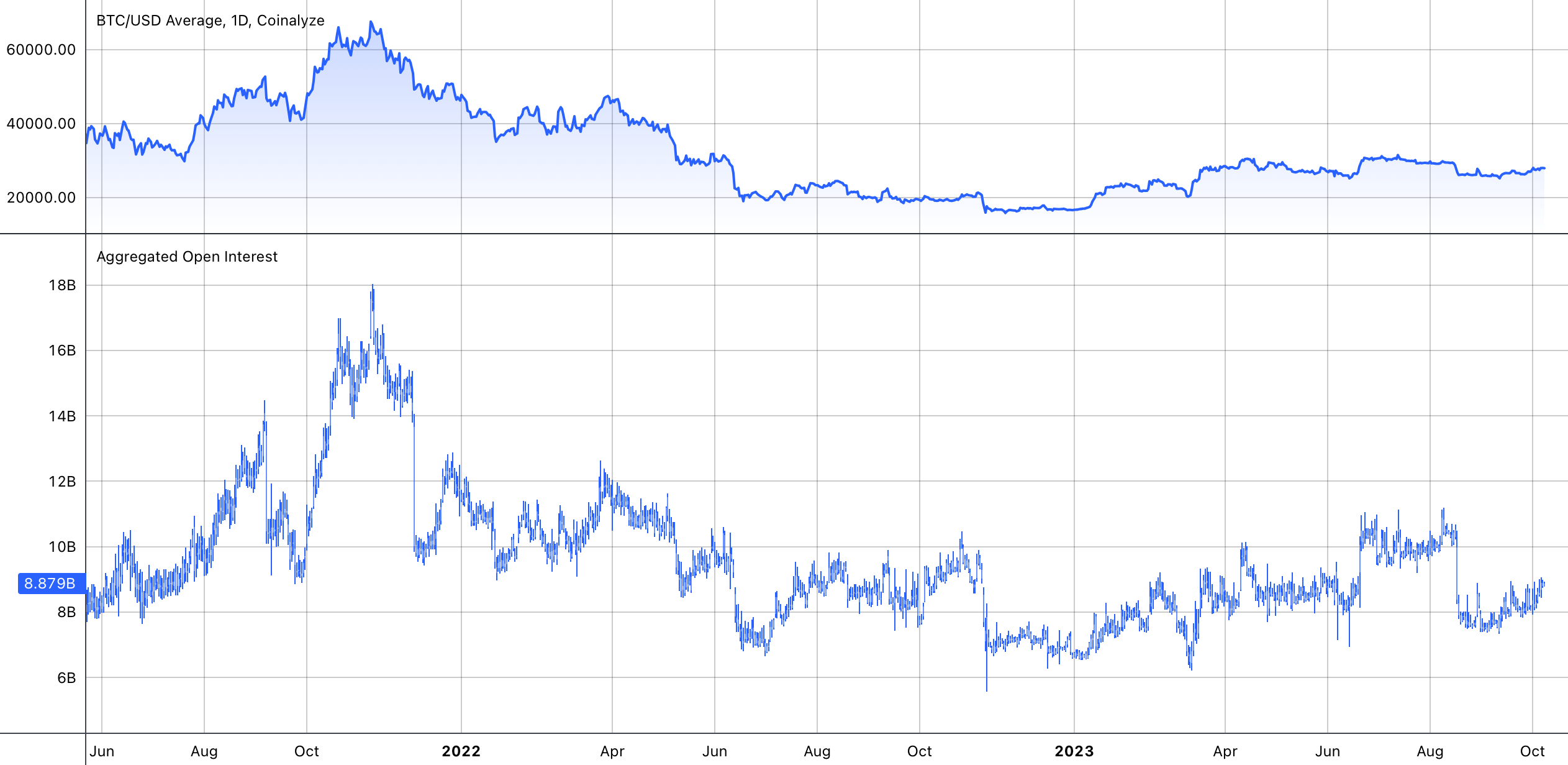
Figure 1: Perpetual Bitcoin futures.

The bottom panels show the evolution of the Bitcoin price and the aggregated open interest in perpetual Bitcoin futures from May 2021 to October 2023. The top panel gives the repartition of open interest across the main trading platforms on October 8, 2023. All data is downloaded from coinalyze.com.

In this paper, we derive the prices of different perpetual futures contracts under the absence of arbitrage. We study discrete-time and continuous-time formulations. We identify funding specifications for the linear and inverse contracts that guarantee that the perpetual future price coincides with the spot so that the basis is constantly equal to zero. In both cases, the required interest term is an easily implementable function of the interest rates in the two currencies. With the assumption of constant funding parameters and interest rates, we derive explicit model-free expressions for the linear and inverse futures prices. We show that, in general, the perpetual future price is the discounted expected value of the future underlying asset’s price at a random time that reflects the funding specification. In the continuous-time case, we provide a general expression for the quanto futures price and use it to obtain a closed-form solution for the required convexity correction in a Black-Scholes setting. Finally, we derive general pricing formulas for everlasting options that we illustrate with closed form solutions for calls and puts in a Black-Scholes setting.

The first case of futures contracts without maturity can be found at the Chinese Gold and Silver Exchange of Hong Kong who developed an undated futures market. However, these contracts did not allow the futures price to fluctuate freely and would instead be settled everyday against the spot price with an interest payment analog to the funding payment. In essence, these undated contracts were automatically rolled over one-day futures contracts, see Gehr Jr (1988) for a discussion. Perpetual futures contracts were formally introduced by Shiller (1993) who proposed the creation of perpetual claims on economic indicators (such as real estate prices and/or corporate profits) where the funding rate would depends on observable cash-flows such as rental rates. While the focus of Shiller (1993) was on real economic indicators rather than cryptocurrencies, his paper laid the groundwork for the subsequent development of perpetual futures. BitMEX is credited with pioneering and popularizing perpetual contracts for cryptocurrencies. In particular, that trading platform introduced inverse contracts in 2016. At the time of writing, perpetual futures are listed on dozens of exchanges and constitute by far the dominant derivatives instrument in that space. For example, of all the listed futures contracts on Bitcoin traded during the first half of 2023, $75\%$ of the 27B USD daily average volume and $94\%$ of the 8B USD daily average open interests can be attributed to perpetual futures.

The literature on the theoretical pricing of perpetual futures contracts is very scarce. Angeris et al. (2023) study a related but different problem in a no-arbitrage framework. They derive the funding rate value such that the perpetual future price is explicitly given by a function of the spot price and the unobservable parameters of the prices process. This type of contract is different from the perpetual future contracts actually traded in cryptocurrency markets, and is not implemented by any exchange at the time of writing. In a recent paper He et al. (2022) derive no-arbitrage prices and bounds for the perpetual futures price, and perform an empirical study of the deviations between their theoretical price and market observations. Their price bounds use a more restrictive definition of the funding rate and rely on a specification of cash flows that is incompatible with the assumption that entering the contract is costless. To the best of our knowledge there is currently no theoretical studies of inverse and quanto contracts. Despite the scarcity of the theoretical literature there are several empirical studies of perpetual futures contracts focusing on price discovery (Alexander et al., 2020), cost of carry (Schmeling et al., 2022; Christin et al., 2023), and market structure (De Blasis and Webb, 2022).

The paper is split in two parts. In the first we consider a discrete-time formulation of a market with two currencies and derive explicit expressions for linear and inverse perpetual futures prices. In the second part we move to a continuous-time formulation in which we derive expressions for linear, inverse, and quantos futures prices that we compare with the recent results of He et al. (2022) and Angeris et al. (2023). Finally, we briefly consider everlasting options and illustrate their pricing within a standard lognormal setting. The proofs of all results are provided in the appendix.

Part I Discrete-time

2 The underlying model

Time is discrete and indexed by $t\in\{0,1,\dots\}$. Uncertainty in the economy is captured by a probability space $(\Omega,{\mathscr{F}},P)$ that we equip with a filtration ${\mathbb{F}}=\{{\mathscr{F}}_{t}\}_{t\geq 0}$. Unless specified otherwise all stochastic processes to appear in what follows are implicitly assumed to be adapted to ${\mathbb{F}}$.

There are two currencies indexed by $i\in\{a,b\}$, for example the US Dollar and Bitcoin. We denote by $x_{t}>0$ the $b/a$ exchange rate at date $t$, that is the price in $a$ of 1 unit of $b$. Investors can freely exchange currencies at this rate and are allowed to invest in two locally risk free bonds: one denominated in units of $a$ and the other in units of $b$. The price of these assets satisfy

$$B_{it+1}=\left(1+r_{it}\right)B_{it},\qquad B_{i0}=1,\qquad i\in\{a,b\},$$ (1)

where $r_{it}>-1$ is the ${\mathscr{F}}_{t}-$measurable return on the $i-$denominated risk free asset over the period from date $t$ to date $t+1$.

To ensure the absence of arbitrages between these two primitive assets, we assume that there exists a probability $Q_{a}$ that is equivalent to $P$ when restricted to ${\mathscr{F}}_{t}$ for any fixed $t\in{\mathbb{N}}$ and such that the price of the $b-$riskless asset expressed in units of $a$ and discounted at the $a-$risk free rate is a martingale under $Q_{a}$:

$$E^{Q_{a}}_{t}\left[\frac{B_{bs}}{B_{as}}x_{s}\right]=\frac{B_{bt}}{B_{at}}x_{t},\qquad\forall t\leq s.$$ (2)

Note that the choice of $a$ as the reference currency is without loss. Indeed, using the strictly positive $Q_{a}-$martingale $\frac{B_{bt}}{B_{at}}\frac{x_{t}}{x_{0}}$ as a density process shows that under the above no-arbitrage assumption there exists a probability $Q_{b}$ that is equivalent to $P$ when restricted to ${\mathscr{F}}_{t}$ for any fixed $t$ and such that

$$E^{Q_{b}}_{t}\left[\frac{B_{as}}{B_{bs}}x^{*}_{s}\right]=\frac{B_{at}}{B_{bt}}x^{*}_{t},\qquad\forall t\leq s,$$ (3)

where $x^{*}_{t}\equiv 1/x_{t}$ denote the $a/b$ exchange rate. We will have the occasion to use both of these currency-specific pricing measures in what follows.

3 Perpetual futures pricing

A perpetual (linear) futures contract provides exposure to one unit of currency $b$ from the point of view of an investor whose unit of account is $a$. Accordingly, the perpetual futures price $f_{t}$ is quoted in units of currency $a$ and all margining operations required by the contract are carried out in that currency.

Entering a contract at date $t$ is costless and, as in a classical futures contract, the long receives at date $t+1$ the one period variation

$$f_{t+1}-f_{t}$$ (4)

in the futures price. If the futures contract had a finite maturity date, say $T$, then this periodic cash flow and the condition that the futures price should equal the spot at maturity are sufficient to uniquely pin down the futures price as the conditional expectation

$$f^{T}_{t}:=E^{Q_{a}}_{t}\left[x_{T}\right]$$ (5)

of the terminal spot price under the $a-$risk neutral probability $Q_{a}$. Without a fixed maturity one needs to introduce additional periodic funding payments to keep the futures price anchored to the spot. The specification of the funding payment varies across exchanges but generally consists in two predictable components: A premium part and an interest part. At date $t+1$ the premium part is

$$\kappa_{t}\left(f_{t}-x_{t}\right)$$ (6)

where the rate $\kappa_{t}>0$ controls the intensity of the anchoring between the spot and the futures price. Intuitively, if the futures price is high relative to the spot at date $t$ then the long will have to pay more at date $t+1$. This in turn makes the long side less attractive and should induce the futures price to move towards the spot. On the other hand, the interest part of the periodic funding payment is given by

$$\iota_{t}x_{t}$$ (7)

where the factor $\iota_{t}$ is set by the exchange to reflect the possibly time varying interest rate differential between the two currencies.

In accordance with these definitions the $a-$denominated cash flow at date $t+1$ from holding a long position over the period from $t$ to $t+1$ is

$$\left(f_{t+1}-f_{t}\right)-\kappa_{t}\left(f_{t}-x_{t}\right)-\iota_{t}x_{t}$$ (8)

and, since entering a futures position is costsless, the absence of arbitrage between the futures, spot, and financial markets requires that

$$E^{Q_{a}}_{t}\left[\left(f_{t+1}-f_{t}\right)-\kappa_{t}\left(f_{t}-x_{t}\right)-\iota_{t}x_{t}\right]=0,\qquad\forall t\geq 0.$$ (9)

Rearranging this equality gives

$$f_{t}=\frac{1}{1+\kappa_{t}}E^{Q_{a}}_{t}\left[f_{t+1}\right]+\left(\frac{\kappa_{t}-\iota_{t}}{1+\kappa_{t}}\right)x_{t}$$ (10)

and iterating this relation forward reveals that

$$f_{t}=E^{Q_{a}}_{t}\left[\left(\prod_{\tau=t}^{T-1}\frac{1}{1+\kappa_{\tau}}\right)f_{T}+\sum_{\sigma=t}^{T-1}\left(\prod_{\tau=t}^{\sigma}\frac{1}{1+\kappa_{\tau}}\right)\left(\kappa_{\sigma}-\iota_{\sigma}\right)x_{\sigma}\right]$$ (11)

for all $t\leq T-1$. To pin down a unique solution to this recursive equation we require that the futures price satisfies the transversality condition:

$$\lim_{T\to\infty}E^{Q_{a}}_{t}\left[\left(\prod_{\tau=t}^{T-1}\frac{1}{1+\kappa_{\tau}}\right)f_{T}\right]=0,\qquad\forall t\geq 0.$$ (12)

Standard arguments then lead to the following results:

Proposition 1.

Assume that

$$E^{Q_{a}}\left[\sum_{\sigma=0}^{\infty}\left(\prod_{\tau=0}^{\sigma}\frac{1}{1+\kappa_{\tau}}\right)\left|\kappa_{\sigma}-\iota_{\sigma}\right|x_{\sigma}\right]<\infty.$$ (13)

Then the process

$$f_{t}=E^{Q_{a}}_{t}\left[\sum_{\sigma=t}^{\infty}\left(\prod_{\tau=t}^{\sigma}\frac{1}{1+\kappa_{\tau}}\right)\left(\kappa_{\sigma}-\iota_{\sigma}\right)x_{\sigma}\right]$$ (14)

is the unique solution to (11) that satisfies condition (12).

Corollary 1.

If $\iota<\kappa$ and $(r_{a},r_{b})$ are constants such that

$$\frac{1}{1+\kappa}\left(\frac{1+r_{a}}{1+r_{b}}\right)<1$$ (15)

then the perpetual futures price

$$f_{t}=\frac{\kappa-\iota}{1+\kappa}\,E^{Q_{a}}_{t}\left[\sum_{\sigma=t}^{\infty}\left(\frac{1}{1+\kappa}\right)^{\sigma-t}x_{\sigma}\right]=\frac{\left(\kappa-\iota\right)\left(1+r_{b}\right)}{r_{b}-r_{a}+\kappa\left(1+r_{b}\right)}x_{t}$$ (16)

is increasing in $r_{a}$ as well as decreasing in $r_{b}$ and $\iota$, and converges monotonically to the spot price as the premium rate $\kappa\to\infty$.

Next, we show that the interest factor $\iota_{t}$ can be chosen by the exchange in such a way that the perpetual futures price and the spot price coincide for any sufficiently large premium rate $\kappa_{t}$ . This result is important from the market design point of view because it delivers a perfect anchoring of the futures price to the spot price through a simple specification of the sole interest factor. It is also important from the financial engineering point of view because if the contract is such that $f_{t}=x_{t}$ then the perpetual futures contract can be dynamically replicated trading in the two primitives assets despite any potential market incompleteness.

Corollary 2.

If the interest factor

$$\iota_{t}=\frac{r_{at}-r_{bt}}{1+r_{bt}}<\kappa_{t}$$ (17)

then the perpetual futures price is equal to the spot price at all times. In this case, the one period cash flow of a long position can be replicated by borrowing

$$m_{t}x_{t}=\frac{x_{t}}{1+r_{bt}}$$ (18)

units of $a$ at rate $r_{at}$ and investing $m_{t}$ units of $b$ at rate $r_{bt}$.

In the standard case of a finite maturity contract the futures price is simply given by the risk-neutral expectation of the terminal spot price under $Q_{a}$ as in (5). Our next result shows that a similar representation holds for the perpetual futures price albeit with a random maturity date whose distribution reflects the funding parameters of the perpetual contract.

Proposition 2.

Assume that (13) holds and that $-1<\iota_{t}<\kappa_{t}$. Then the perpetual futures price satisfies

$$f_{t}=E^{Q_{a}}_{t}\left[\left(\prod_{\tau=t}^{\theta_{t}-1}\frac{1}{1+\iota_{\tau}}\right)x_{\theta_{t}}\right]$$ (19)

where $\theta_{t}\geq t$ is a random time that is defined on an extension of the probability space and distributed according to

$$Q_{a}\left(\theta_{t}=\sigma\middle|{\mathscr{F}}\right)=\mathbf{1}_{\left\{t\leq\sigma\right\}}\frac{\kappa_{\sigma}-\iota_{\sigma}}{1+\iota_{\sigma}}\left(\prod_{\tau=t}^{\sigma}\frac{1+\iota_{\tau}}{1+\kappa_{\tau}}\right).$$ (20)

In particular, if the premium rate $\kappa$ is constant and the interest factor $\iota\equiv 0$ then the perpetual futures price is simply given by

$$f_{t}=E^{Q_{a}}_{t}\left[\sum_{n=0}^{\infty}\kappa\left(1+\kappa\right)^{-(n+1)}x_{t+n}\right]=E^{Q_{a}}_{t}\left[x_{t+\eta}\right]$$ (21)

where $\eta$ is a geometrically distributed random time with mean $1/\kappa$.

4 Inverse futures pricing

The inverse perpetual futures contract offers an exposure to the $b/a$ exchange rate and is quoted in units of currency $a$ but, unlike the linear contract, its margined and funded in currency $b$. This alternative form of futures contract is particularly well suited to crypto-currency investors. Indeed, the fact that the contract operates entirely in the target currency, say Bitcoin or Ether, implies that it can be run entirely on chain without ever having to own or transfer any units of fiat money.

The contract size is expressed in units of $a$ and fixed to one. As a result, the $b-$denominated cash flow at date $t+1$ from holding a long position in the inverse perpetual futures over the period from date $t$ to date $t+1$ is

$$\left(\frac{1}{f_{It+1}}-\frac{1}{f_{It}}\right)-\kappa_{It}\left(\frac{1}{f_{It}}-x^{*}_{t}\right)-\iota_{It}x^{*}_{t}$$ (22)

where $f_{It}$ denotes the inverse perpetual futures price quoted in units of $a$, $x^{*}_{t}=1/x_{t}$ denotes the price of one unit of $a$ in units of $b$, and $(\iota_{It},\kappa_{It})$ are contract-specific adapted funding parameters set by the exchange. Since entering an inverse futures position is costless, the absence of arbitrage requires that

$$E^{Q_{b}}_{t}\left[\left(\frac{1}{f_{It+1}}-\frac{1}{f_{It}}\right)-\kappa_{It}\left(\frac{1}{f_{It}}-x^{*}_{t}\right)-\iota_{It}x^{*}_{t}\right]=0,\qquad\forall t\geq 0,$$ (23)

where $Q_{b}$ is the pricing measure for $b-$denominated cash flows. Rearranging this identity we find that

$$\frac{1}{f_{It}}=\frac{1}{1+\kappa_{It}}E^{Q_{b}}_{t}\left[\frac{1}{f_{It+1}}\right]+\left(\frac{\kappa_{It}-\iota_{It}}{1+\kappa_{It}}\right)x^{*}_{t}$$ (24)

and iterating this relation forward reveals that

$$\frac{1}{f_{It}}=E^{Q_{b}}_{t}\left[\left(\prod_{\tau=t}^{T-1}\frac{1}{1+\kappa_{I\tau}}\right)\frac{1}{f_{IT}}+\sum_{\sigma=t}^{T-1}\left(\prod_{\tau=t}^{\sigma}\frac{1}{1+\kappa_{I\tau}}\right)\left(\kappa_{I\sigma}-\iota_{I\sigma}\right)x^{*}_{\sigma}\right].$$ (25)

for all $t+1\leq T$. As in the linear case, we single out a natural solution to this recursive equation by imposing the transversality condition

$$\lim_{T\to\infty}E^{Q_{b}}_{t}\left[\left(\prod_{\tau=t}^{T-1}\frac{1}{1+\kappa_{I\tau}}\right)\frac{1}{f_{IT}}\right]=0,\qquad\forall t\geq 0.$$ (26)

Arguments similar to those of Section 4 then deliver the following counterparts of Propositions 1–2 and Corollaries 1–2 for the inverse contract.

Proposition 3.

Assume that

$$E^{Q_{b}}\left[\sum_{\sigma=0}^{\infty}\left(\prod_{\tau=0}^{\sigma}\frac{1}{1+\kappa_{I\tau}}\right)\left|\kappa_{I\sigma}-\iota_{I\sigma}\right|x^{*}_{\sigma}\right]<\infty.$$ (27)

Then the process

$$\frac{1}{f_{It}}=E^{Q_{b}}_{t}\left[\sum_{\sigma=t}^{\infty}\left(\prod_{\tau=t}^{\sigma}\frac{1}{1+\kappa_{I\tau}}\right)\left(\kappa_{I\sigma}-\iota_{I\sigma}\right)x^{*}_{\sigma}\right]$$ (28)

is the unique solution to (25) that satisfies condition (26).

Corollary 3.

If the interest factor

$$\iota_{It}=\frac{r_{bt}-r_{at}}{1+r_{at}}<\kappa_{It}$$ (29)

then the perpetual inverse futures price is equal to the spot price. In this case, the one period cash flow of a long position can be replicated by borrowing

$$m_{It}x^{*}_{t}=\frac{x^{*}_{t}}{1+r_{at}}$$ (30)

units of $b$ at rate $r_{bt}$ and investing $m_{It}$ units of $a$ at rate $r_{at}$.

Corollary 4.

If $\iota_{I}<\kappa_{I}$ and $(r_{a},r_{b})$ are constants such that

$$\frac{1}{1+\kappa_{I}}\left(\frac{1+r_{b}}{1+r_{a}}\right)<1$$ (31)

then the perpetual inverse futures price

$$f_{It} =\frac{r_{a}-r_{b}+\kappa_{I}\left(1+r_{a}\right)}{\left(\kappa_{I}-\iota_{I}\right)\left(1+r_{a}\right)}x_{t}$$ (32)

is decreasing in $r_{b}$ as well as increasing in $r_{a}$ and $\iota_{I}$, and converges monotonically to the spot price as the premium rate $\kappa_{I}\to\infty$.

Proposition 4.

Assume that (27) holds and that $-1<\iota_{It}<\kappa_{It}$. Then the perpetual futures price satisfies

$$\frac{1}{f_{It}}=E^{Q_{b}}_{t}\left[\left(\prod_{\tau=t}^{\theta_{It}-1}\frac{1}{1+\iota_{I\tau}}\right)x^{*}_{\theta_{It}}\right]$$ (33)

where $\theta_{It}\geq t$ is a random time that is defined on an extension of the probability space and distributed according to

$$Q_{b}\left(\theta_{It}=\sigma\middle|{\mathscr{F}}\right)=\mathbf{1}_{\left\{t\leq\sigma\right\}}\frac{\kappa_{I\sigma}-\iota_{I\sigma}}{1+\iota_{I\sigma}}\left(\prod_{\tau=t}^{\sigma}\frac{1+\iota_{I\tau}}{1+\kappa_{I\tau}}\right).$$ (34)

In particular, if the premium rate $\kappa_{I}$ is constant and the interest factor $\iota_{I}\equiv 0$ then the perpetual inverse futures price is simply given by

$${f_{It}}={E^{Q_{b}}_{t}\left[x^{*}_{t+\eta_{I}}\right]}^{-1}$$ (35)

where $\eta_{I}$ is a geometrically distributed random time with mean $1/\kappa_{I}$.

Part II Continuous-time

5 The model

Time is continuous and indexed by $t\geq 0$. Uncertainty is represented by a filtered probability space $(\Omega,{\mathscr{F}},{\mathbb{F}},P)$ where the filtration is right continuous and such that ${\mathscr{F}}=\cap_{t\geq 0}{\mathscr{F}}_{t}$. Unless specified otherwise all processes to appear in what follows are assumed to be adapted to the filtration ${\mathbb{F}}$.

As in discrete-time, there are two currencies $i\in\{a,b\}$ and we denote by $x_{t}$ the $b/a$ exchange rate at date $t$. Investors can freely exchange currencies at this rate and are allowed to invest in two locally riskless assets: one denominated in units of $a$ and the other in units of $b$. The price of these assets satisfy

$$dB_{it}=r_{it}B_{it}dt,\qquad B_{i0}=1,\qquad i\in\{a,b\}$$ (36)

where $r_{it}>-1$ captures the return on the $i-$denominated asset over an infinitesimal time interval starting at date $t$. To ensure the absence of arbitrages between these primitive assets we assume that there exists a probability $Q_{a}$ that is equivalent to $P$ when restricted to ${\mathscr{F}}_{t}$ for any finite $t$ and such that (2) holds for all real $t\leq s$; and we note that, as in the discrete-time formulation, this assumption implies the existence of a probability $Q_{b}$ that is equivalent to $P$ when restricted to ${\mathscr{F}}_{t}$ for any finite $t$ and such that (3) is satisfied for all real $t\leq s$.

6 Linear futures pricing

Let $\tau\leq\sigma$ be stopping times. In view of the single period cash flow in (8) it is clear that the cumulative $a-$discounted cash flows from holding a long position in a perpetual futures contract over $[\![\tau,\sigma]\!]$ are given by

$$\int_{\tau}^{\sigma}\frac{dC_{t}}{B_{at}}=\int_{\tau}^{\sigma}\frac{1}{B_{at}}\left(df_{t}-\left(\iota_{t}x_{t}+\kappa_{t}\left(f_{t}-x_{t}\right)\right)dt\right)$$ (37)

where the premium rate $\kappa_{t}>0$ and the interest factor $\iota_{t}$ are set by the exchange. Since a position in the contract can be opened or closed without cost at any point in time, the absence of arbitrage requires that

$$E^{Q_{a}}_{\tau}\left[\int_{\tau}^{\sigma}\frac{dC_{t}}{B_{at}}\right]=0,\qquad\forall\tau\leq\sigma\in{\mathscr{S}}$$ (38)

where ${\mathscr{S}}$ denotes the set of stopping times of the filtration. Rearranging this equality shows that the process

$$M_{t}:=\int_{0}^{t}\frac{dC_{s}}{B_{as}}$$ (39)

is a martingale under $Q_{a}$. This in turn implies that $C_{t}$ is a local martingales under $Q_{a}$ and substituting the definition of the cumulative cash flow process reveals that the perpetual futures prices evolves according to

$$df_{t}=B_{at}dM_{t}+\left(\iota_{t}x_{t}+\kappa_{t}\left(f_{t}-x_{t}\right)\right)dt.$$ (40)

Finally, discounting at the premium rate $\kappa_{t}$ on both sides and integrating the resulting expression shows that

$$e^{-\int_{0}^{t}\kappa_{u}du}f_{t}+\int_{0}^{t}e^{-\int_{0}^{s}\kappa_{u}du}\left(\iota_{s}-\kappa_{s}\right)x_{s}ds\in\mathscr{M}_{\mathrm{loc}}(Q_{a})$$ (41)

where $\mathscr{M}_{\mathrm{loc}}(Q_{a})$ denotes the set of $Q_{a}-$local martingales. As in discrete-time, one can single out a unique process satisfying this restriction by imposing a transversality condition which here takes the following form:

$$\lim_{\sigma\to\infty}E^{Q_{a}}_{t}\left[e^{-\int_{0}^{\sigma_{n}}\kappa_{u}du}f_{\sigma_{n}}\right]=0,\qquad\forall t\geq 0\text{ and }(\sigma_{n})_{n=1}^{\infty}\subset{\mathscr{S}}\text{ s.t. }\sigma_{n}\uparrow\infty.$$ (42)

Classical arguments then lead to the following continuous-time versions of the results of Propositions 1–2 and Corollaries 1–2. While the proofs are slightly more involved in continuous-time we stress that the results themselves are the exact counterparts of the discrete-time results.

Proposition 5.

Assume that

$$E^{Q_{a}}\left[\int_{0}^{\infty}e^{-\int_{0}^{s}\kappa_{u}du}\left|\kappa_{s}-\iota_{s}\right|x_{s}ds\right]<\infty.$$ (43)

Then

$$f_{t}=E^{Q_{a}}_{t}\left[\int_{t}^{\infty}e^{-\int_{t}^{s}\kappa_{u}du}\left(\kappa_{s}-\iota_{s}\right)x_{s}ds\right]$$ (44)

is the unique process that satisfies both (41) and (42).

Corollary 5.

If $\iota<\kappa$ and $(r_{a},r_{b})$ are constants such that $\kappa+r_{b}-r_{a}>0$ then the perpetual futures price

$$f_{t}=\frac{\left(\kappa-\iota\right)}{\kappa+r_{b}-r_{a}}x_{t}$$ (45)

is increasing in $r_{a}$ as well as decreasing in $r_{b}$ and $\iota$, and converges monotonically to the spot price as the premium rate $\kappa\to\infty$.

In a contemporaneous paper He, Manela, Ross, and von Wachter (2022) show that in a continuous-time setting with constant parameters and $r_{b}=\iota\equiv 0$ the perpetual futures price is given by $\left(1+\frac{r_{a}}{\kappa}\right)x_{t}$ which is clearly different from the prescription of Corollary 5. The reason for this discrepancy is that the specification considered by He et al. (2022) if different from ours and, in fact, inconsistent with the assumption that entering a contract is costless unless $r_{a}\equiv 0$. Specifically, He et al. (2022, Definition 1 and Table 1) assume that the discounted payoff generated by holding a long position in one unit of the contract between two stopping times $\tau$ and $\sigma$ is

$$e^{-r_{a}\sigma}\left(F_{\sigma}-F_{\tau}\right)-\int_{\tau}^{\sigma}{e^{-r_{a}s}\kappa\left(F_{s}-x_{s}\right)ds}.$$ (46)

If entering the contract is costless then the value of this payoff at date $\tau$ should be zero for all stopping times $\tau\leq\sigma$, i.e. we should have

$$E^{Q_{a}}_{\tau}\left[e^{-r_{a}\sigma}\left(F_{\sigma}-F_{\tau}\right)-\int_{\tau}^{\sigma}{e^{-r_{a}s}\kappa\left(F_{s}-x_{s}\right)ds}\right]=0,\qquad\tau\leq\sigma\in{\mathscr{S}}.$$ (47)

But this restriction implies that

$$M_{t}(T)=F_{t\wedge T}-\int_{0}^{t\wedge T}e^{r_{a}(T-s)}\kappa\left(F_{s}-x_{s}\right)ds$$ (48)

is a martingale under $Q_{a}$ for any $T<\infty$ which is not possible if $r_{a}\neq 0$. Indeed, if that property was satisfied then the difference

$$M_{t}(T)-M_{t}(T+h)=\int_{0}^{t}\left(e^{r_{a}(T-s)}-e^{r_{a}(T+h-s)}\right)\kappa\left(F_{s}-x_{s}\right)ds$$ (49)

would be a continuous $Q_{a}-$martingale of finite variation on $[0,T]$ and thus a constant. If $r_{a}=0$ then this is not a problem. However, if $r_{a}\neq 0$ then the constancy of the above difference requires that $F_{t}=x_{t}$ which is inconsistent with (47) because the exchange rate cannot be a martingale under $Q_{a}$ when $r_{a}\neq 0=r_{b}$. Intuitively, the problem in the specification of He et al. (2022) is that, instead of being paid continuously over time, the margin $F_{\sigma}-F_{\tau}$ is paid in a lumpsum upon exiting the contract.

Corollary 6.

Assume that

$$\iota_{t}\equiv r_{at}-r_{bt}<\kappa_{t}$$ (50)

then the perpetual futures price is equal to the spot price at all times and can be dynamically replicated by trading in the two riskless assets.

Proposition 6.

Assume that condition (43) holds and that $\iota_{t}<\kappa_{t}$. Then the perpetual futures price can be expressed as

$$f_{t}=E^{Q_{a}}_{t}\left[e^{-\int_{t}^{\theta_{t}}\iota_{u}du}x_{\theta_{t}}\right]$$ (51)

where $\theta_{t}\geq t$ is a random time that is defined on an extension of the probability space and distributed according to

$$Q_{a}\left(\theta_{t}\in ds\middle|{\mathscr{F}}\right)=\mathbf{1}_{\left\{s\geq t\right\}}e^{-\int_{t}^{s}(\kappa_{u}-\iota_{u})du}\left(\kappa_{s}-\iota_{s}\right)ds,\qquad s\geq 0.$$ (52)

In particular, if the premium rate $\kappa$ is constant and the interest factor $\iota\equiv 0$ then the perpetual futures price is simply given by

$$f_{t}=E^{Q_{a}}_{t}\left[\int_{t}^{\infty}\kappa e^{-\kappa(s-t)}x_{s}ds\right]=E^{Q_{a}}_{t}\left[x_{t+\tau}\right]$$ (53)

where $\tau$ is an exponentially distributed random time with mean $1/\kappa$.

7 Inverse and quanto futures pricing

Perpetual inverse futures.

Let $x^{*}_{t}:=1/x_{t}$ denote the price of one unit of $a$ in units of $b$ and recall that $Q_{b}$ is the pricing measure for $b-$denominated cash flows. Proceeding as in the case of the linear contract shows that the arbitrage restriction for the inverse contract is given by

$$E^{Q_{b}}_{\tau}\left[\int_{\tau}^{\sigma}\frac{dC_{it}}{B_{bt}}\right]=0,\qquad\forall\tau\leq\sigma\in{\mathscr{S}},$$ (54)

where the incremental cash flow

$$dC_{it}=d\left(\frac{1}{f_{It}}\right)-\kappa_{It}\left(\frac{1}{f_{It}}-x^{*}_{t}\right)dt-\iota_{It}x^{*}_{t}dt$$ (55)

is denominated in units of $b$ and the parameters $(\iota_{It},\kappa_{It})$ are set by the exchange subject to $\kappa_{It}>0$. The same arguments as in the linear case then imply that

$$e^{-\int_{0}^{t}\kappa_{Iu}du}\frac{1}{f_{It}}+\int_{0}^{t}e^{-\int_{0}^{s}\kappa_{Iu}du}\left(\iota_{Iu}-\kappa_{Iu}\right)x^{*}_{s}ds\in\mathscr{M}_{\mathrm{loc}}(Q_{b})$$ (56)

and imposing the transversality condition

$$\lim_{\sigma\to\infty}E^{Q_{b}}_{t}\left[e^{-\int_{0}^{\sigma_{n}}\kappa_{Iu}du}\frac{1}{f_{I\sigma_{n}}}\right]=0,\qquad\forall t\geq 0\text{ and }(\sigma_{n})_{n=1}^{\infty}\subset{\mathscr{S}}\text{ s.t. }\sigma_{n}\uparrow\infty$$ (57)

allows to uniquely determine the inverse futures price. In particular, we have the following counterparts to Propositions 5–6 and Corollaries 5–6.

Proposition 7.

Assume that

$$E^{Q_{b}}\left[\int_{0}^{\infty}e^{-\int_{0}^{s}\kappa_{Iu}du}\left|\kappa_{Is}-\iota_{Is}\right|x^{*}_{s}ds\right]<\infty.$$ (58)

Then the process

$$\frac{1}{f_{It}}=E^{Q_{b}}_{t}\left[\int_{t}^{\infty}e^{-\int_{t}^{s}\kappa_{Iu}du}\left(\kappa_{Is}-\iota_{Is}\right)x^{*}_{s}ds\right]$$ (59)

is the unique solution to (56) that satisfies condition (42).

Corollary 7.

If the interest factor

$$\iota_{It}=r_{bt}-r_{at}<\kappa_{t}$$ (60)

then the perpetual inverse futures price equals the spot price at all times and can be dynamically replicated by trading in the two riskless assets.

Corollary 8.

If $\iota_{I}<\kappa_{I}$ and $(r_{a},r_{b})$ are constants such that $\kappa_{I}+r_{a}-r_{b}>0$ then the perpetual inverse futures price

$$f_{It}=\frac{\left(\kappa_{I}+r_{a}-r_{b}\right)}{\kappa_{I}-\iota_{I}}x_{t}$$ (61)

is decreasing in $r_{b}$ as well as increasing in $r_{a}$ and $\iota$, and converges monotonically to the spot price as the premium rate $\kappa_{I}\to\infty$.

Proposition 8.

Assume that (58) holds and that $\iota_{It}<\kappa_{It}$. Then the perpetual futures price can be expressed as

$$\frac{1}{f_{It}}=E^{Q_{b}}_{t}\left[e^{-\int_{t}^{\theta_{It}}\iota_{Iu}du}x^{*}_{\theta_{It}}\right]$$ (62)

where $\theta_{It}\geq t$ is a random time that is defined on an extension of the probability space and distributed according to

$$Q_{b}\left(\theta_{It}\in ds\middle|{\mathscr{F}}\right)=\mathbf{1}_{\left\{t\leq s\right\}}e^{-\int_{t}^{s}(\kappa_{Iu}-\iota_{Iu})du}\left(\kappa_{Is}-\iota_{Is}\right)ds,\qquad s\geq 0.$$ (63)

In particular, if the premium rate $\kappa_{I}$ is constant and the interest factor $\iota_{I}\equiv 0$ then the perpetual inverse futures price is simply given by

$$\frac{1}{f_{It}}=E^{Q_{b}}_{t}\left[\int_{t}^{\infty}\kappa_{I}e^{-\kappa_{I}(s-t)}x^{*}_{s}ds\right]=E^{Q_{b}}_{t}\left[x^{*}_{t+\tau_{i}}\right]$$ (64)

where $\tau_{i}$ is an exponentially distributed random time with mean $1/\kappa_{I}$.

Perpetual quanto futures.

Let now $c$ denote a third currency. Quanto futures are contracts that give exposure to the $c/a$ exchange rate $z_{t}>0$ but are quoted, margined, and funded using currency $b$. Specifically, the size of the contract is set to one unit of $c$ and the periodic cash flows are computed in units of $a$ but paid in units $b$ after conversion using a constant $a/b$ exchange rate $\chi^{*}$ specified in the contract.

Accordingly, the instantaneous cash flow in units of $b$ from a long position in the perpetual quanto futures contract is

$$dC_{qt}=\chi^{*}df_{qt}-\chi^{*}\left(\iota_{qt}z_{t}+\kappa_{qt}\left({f_{qt}}-z_{t}\right)\right)dt$$ (65)

where the funding parameters $(\iota_{qt},\kappa_{qt})$ are set by the exchange subject to $\kappa_{qt}>0$, and the absence of arbitrage requires that

$$\chi^{*}E^{Q_{b}}_{\tau}\left[\int_{\tau}^{\sigma}\frac{dC_{qt}}{B_{bt}}\right]=0,\qquad\forall\tau\leq\sigma\in{\mathscr{S}}.$$ (66)

Proceeding as in the linear case then shows that

$$e^{-\int_{0}^{t}\kappa_{qu}du}f_{qt}+\int_{0}^{t}e^{-\int_{0}^{s}\kappa_{qu}du}\left(\iota_{qu}-\kappa_{qu}\right)z_{s}ds\in\mathscr{M}_{\mathrm{loc}}(Q_{b}),$$ (67)

and imposing the transversality condition

$$\lim_{\sigma\to\infty}E^{Q_{b}}_{t}\left[e^{-\int_{0}^{\sigma_{n}}\kappa_{qu}du}{f_{q\sigma_{n}}}\right]=0,\qquad\forall t\geq 0\text{ and }(\sigma_{n})_{n=1}^{\infty}\subset{\mathscr{S}}\text{ s.t. }\sigma_{n}\uparrow\infty$$ (68)

allows to uniquely determine the quanto futures price.

Proposition 9.

Assume that

$$E^{Q_{b}}\left[\int_{0}^{\infty}e^{-\int_{0}^{s}\kappa_{qu}du}\left|\kappa_{qs}-\iota_{qs}\right|z_{s}ds\right]<\infty.$$ (69)

Then the process

$$f_{qt}=E^{Q_{b}}_{t}\left[\int_{t}^{\infty}e^{-\int_{t}^{s}\kappa_{qu}du}\left(\kappa_{qs}-\iota_{qs}\right)z_{s}ds\right]$$ (70)

is the unique solution to (56) that satisfies condition (42). If, furthermore, $\kappa_{qt}-\iota_{qt}>0$ then the perpetual quanto futures price can expressed as

$$E^{Q_{b}}_{t}\left[e^{-\int_{t}^{\theta_{qt}}\iota_{qu}du}z_{\theta_{qt}}\right]$$ (71)

where $\theta_{qt}\geq t$ is a random time that is defined on an extension of the probability space and distributed according to

$$Q_{b}\left(\theta_{qt}\in ds\middle|{\mathscr{F}}\right)=\mathbf{1}_{\left\{t\leq s\right\}}e^{-\int_{t}^{s}(\kappa_{qu}-\iota_{qu})du}\left(\kappa_{qs}-\iota_{qs}\right)ds,\qquad s\geq 0.$$ (72)

In particular, if the premium rate $\kappa_{q}$ is constant and the interest factor $\iota_{q}\equiv 0$ then the perpetual quanto futures price is simply given by

$$f_{qt}=E^{Q_{b}}_{t}\left[\int_{t}^{\infty}\kappa_{q}e^{-\kappa_{q}(s-t)}z_{s}ds\right]=E^{Q_{b}}_{t}\left[z_{t+\tau_{q}}\right]$$ (73)

where $\tau_{q}$ is an exponentially distributed random time with mean $1/\kappa_{q}$.

In contrast to the linear and inverse cases it is no longer possible to obtain explicit expressions for the futures price or the equalizing interest factor without specifying a model for the exchange rates $z_{t}$ and $x_{t}$. This difficulty arises from the fact that $z_{t}$ applies to the currency pair $c/a$ and thus is unrelated to currency $b$. As a result, its drift under $Q_{b}$ depends on the covariance between changes in $z_{t}$ and changes in the $b/a$ exchange rate $x_{t}$, and this covariance can only be computed once we specify the sources of risk that affect theses processes.

To illustrate this convexity adjustment assume that $r_{a},r_{b},r_{c},\iota_{q},\kappa_{q}$ are constants and that the pair $(x_{t},z_{t})$ evolves according to

$$dx_{t}/x_{t}=\left(r_{a}-r_{b}\right)dt+\sigma_{x}^{*}dZ_{at}$$ (74)

$$dz_{t}/z_{t}=\left(r_{a}-r_{c}\right)dt+\sigma_{z}^{*}dZ_{at}$$ (75)

where $r_{c}$ is the constant interest rate that applies to $c-$denominated riskfree deposits and loans, $(\sigma_{x},\sigma_{z})$ are constant vectors of dimension $n$, and $Z_{at}$ is a $n-$dimensional Brownian under measure $Q_{a}$. Since

$$\left.\frac{dQ_{b}}{dQ_{a}}\right|_{{\mathscr{F}}_{t}}=e^{(r_{b}-r_{a})t}\frac{x_{t}}{x_{0}}=e^{-\frac{1}{2}\|\sigma_{x}\|^{2}t+\sigma_{x}^{*}Z_{at}}$$ (76)

it follows from Girsanov’s theorem that

$$dz_{t}/z_{t}=\left(r_{a}-r_{c}+\sigma_{x}^{*}\sigma_{z}\right)dt+\sigma_{z}^{*}dZ_{bt}$$ (77)

where $Z_{bt}$ is an $n-$dimensional Brownian under $Q_{b}$ and using this evolution allows to derive the following result:

Proposition 10.

Assume that $\iota_{q}<\kappa_{q}$ and $\kappa_{q}+r_{c}-r_{a}-\sigma_{x}^{*}\sigma_{z}>0$. Then the perpetual quanto futures price

$$f_{qt}=\frac{\left(\kappa_{q}-\iota_{q}\right)z_{t}}{\kappa_{q}+r_{c}-r_{a}-\sigma_{x}^{*}\sigma_{z}}$$ (78)

is decreasing in $r_{c}$ and $\iota_{q}$ as well as increasing in $r_{a}$ and $\sigma_{x}^{*}\sigma_{z}$, and converges monotonically to the spot price as the premium rate $\kappa_{q}\to\infty$.

8 Everlasting options

Everlasting options work in a similar manner as perpetual futures but track a function of the spot price instead of the spot price itself. The idea and the name seem to go back to Bankman-Fried and White (2021) and some specifications, such as quadratic perpetuals, are traded on some exchanges. See, for example Prospere (2022). Note however that the name can be misleading: Everlasting options are actually not options but perpetual future contracts. In particular, an everlasting call or put option is very different from a perpetual American option.

Let $\varphi:{\mathbb{R}}_{+}\to{\mathbb{R}}$ denote a payoff function. The futures price for the corresponding everlasting option is quoted and margined in units of $a$. As a result, the cumulative cash flows from holding a long position evolves according to

$$dC_{ot}=df_{ot}-\kappa_{ot}\left(f_{ot}-\varphi(x_{t})\right)dt$$ (79)

where $f_{ot}$ denotes the (futures) price of the everlasting option and $\kappa_{ot}>0$ is a premium rate set by the exchange. The same arguments as in the linear case then imply that the absence of arbitrage requires that

$$e^{-\int_{0}^{t}\kappa_{Iu}du}f_{ot}+\int_{0}^{t}e^{-\int_{0}^{s}\kappa_{Iu}du}\kappa_{os}\varphi\left(x_{s}\right)ds\in\mathscr{M}_{\mathrm{loc}}(Q_{a})$$ (80)

and imposing the transversality condition

$$\lim_{\sigma\to\infty}E^{Q_{a}}_{t}\left[e^{-\int_{0}^{\sigma_{n}}\kappa_{ou}du}f_{o\sigma_{n}}\right]=0,\qquad\forall t\geq 0\text{ and }(\sigma_{n})_{n=1}^{\infty}\subset{\mathscr{S}}\text{ s.t. }\sigma_{n}\uparrow\infty$$ (81)

allows to uniquely determine the inverse futures price.

Proposition 11.

Assume that

$$E^{Q_{a}}\left[\int_{0}^{\infty}e^{-\int_{0}^{s}\kappa_{ou}du}\kappa_{qs}x_{s}ds\right]<\infty.$$ (82)

Then the process

$$f_{ot}=E^{Q_{b}}_{t}\left[\int_{t}^{\infty}e^{-\int_{t}^{s}\kappa_{ou}du}\kappa_{os}x_{s}ds\right]$$ (83)

is the unique solution to (80) that satisfies condition (81). Furthermore, this unique solution can be expressed as

$$f_{ot}=E^{Q_{a}}_{t}\left[\varphi\left(x_{\theta_{ot}}\right)\right]$$ (84)

where $\theta_{ot}\geq t$ is a random time that is defined an extension of the probability space and distributed according to

$$Q_{a}\left(\theta_{ot}\in ds\middle|{\mathscr{F}}\right)=\mathbf{1}_{\left\{t\leq s\right\}}e^{-\int_{t}^{s}\kappa_{ou}du}\kappa_{os}ds,\qquad s\geq 0.$$ (85)

In particular, if $\kappa_{o}$ is constant then

$$f_{ot}=E^{Q_{a}}_{t}\left[\int_{t}^{\infty}\kappa_{o}e^{-\kappa_{o}(s-t)}\varphi\left(x_{s}\right)ds\right]=E^{Q_{a}}_{t}\left[\varphi\left(x_{t+\tau_{o}}\right)\right]$$ (86)

where $\tau_{o}$ is an exponentially distributed random time with mean $1/\kappa_{o}$.

In a recent paper, Angeris et al. (2023) study an inverse problem that is related to Corollary 6. However, their results are not directly comparable to ours because the contract that they analyze is different. Indeed, they consider an $a-$denominated perpetual contract which the long pays some amount $\Phi_{\tau}$ upon entering the contract at date $\tau$ as well as funding at some rate $F_{t}dt$ and receives the amount $\Phi_{\sigma}$ upon exiting the contract at date $\sigma\geq\tau$. In this specification, the cumulative net discounted cash flow to the long over the holding period is

$$N:=\frac{\Phi_{\sigma}}{B_{a\sigma}}-\frac{\Phi_{\tau}}{B_{a\tau}}-\int_{\tau}^{\sigma}{\frac{F_{s}}{B_{as}}ds}=\int_{\tau}^{\sigma}d\left(\frac{\Phi_{s}}{B_{as}}\right)-\int_{\tau}^{\sigma}{\frac{F_{s}}{B_{as}}ds}.$$ (87)

By contrast, in our formulation the cumulative discounted cash flows from holding a long position in the corresponding perpetual futures would be

$$\int_{\tau}^{\sigma}\left(\frac{d\Phi_{s}}{B_{as}}-\frac{F_{s}}{B_{as}}ds\right)=N+\int_{\tau}^{\sigma}r_{as}\frac{\Phi_{s}}{B_{as}}ds$$ (88)

because the contract is margined continuously rather than only at the beginning and end. We believe that our formulation more closely reflects the actual functioning of markets because in practice contracts do not require an upfront payment.

Within our formulation, the problem analyzed by Angeris et al. (2023) consists in determining the funding rate $F_{t}$ in such a way that the associated perpetual futures price $\Phi_{t}=\varphi(x_{t})$ at all times for some given function. If the exchange rate follows an Itô process as in their paper, then (2) implies that

$$dx_{t}=\left(r_{at}-r_{bt}\right)x_{t}dt+\Sigma_{xt}^{*}dZ_{at}$$ (89)

for some diffusion coefficient $\Sigma_{xt}$ and some $Q_{a}-$Brownian motion $Z_{at}$ of the same dimension. In this case, the problem can be solved by a direct application of Itô’s lemma. Indeed, if $\varphi\in C^{2}$ then the funding rate

$$F_{t}(\varphi):=\varphi^{\prime}(x_{t})\left(r_{at}-r_{bt}\right)x_{t}+\frac{1}{2}\varphi^{\prime\prime}(x_{t})\|\Sigma_{xt}\|^{2}$$ (90)

has the property that

$$\int_{0}^{t}\frac{1}{B_{as}}\left(d\varphi(x_{s})-F_{s}(\varphi)\right)ds\in\mathscr{M}_{\mathrm{loc}}(Q_{a}).$$ (91)

Under appropriate integrability assumptions on $\varphi(x_{t})$ this local martingale property in turn implies that

$$E^{Q_{a}}_{\tau}\left[\int_{\tau}^{\sigma}\frac{1}{B_{as}}\left(d\varphi(x_{s})-F_{s}(\varphi)\right)ds\right]=0,\qquad\forall\tau\leq\sigma\in{\mathscr{S}},$$ (92)

and it follows that $\varphi(x_{t})$ is the futures price induced by the funding rate $F_{t}(\varphi)$. In particular, for the identity function we find that

$$F_{t}(\varphi)=\left(r_{at}-r_{bt}\right)x_{t}$$ (93)

from which we recover the result of Corollary 6. Note however that the latter corollary was proved without any assumption on the evolution of the exchange rate other than the no-arbitrage condition.

To illustrate the pricing of everlasting options, assume the exchange rate evolves according to (74) and consider the call and put options with premium rate $\kappa>0$. The associated prices are given by

$${c_{t}} =E^{Q_{a}}_{t}\left[\int_{t}^{\infty}\kappa e^{-\kappa(s-t)}\left({x}_{s}-K\right)^{+}ds\right],$$ (94)

$${p_{t}} =E^{Q_{a}}_{t}\left[\int_{t}^{\infty}\kappa e^{-\kappa(s-t)}\left({K}-x_{s}\right)^{+}ds\right],$$ (95)

and satisfy the everlasting put-call parity

$${c_{t}-p_{t}} =E^{Q_{a}}\left[\int_{t}^{\infty}\kappa e^{-\kappa(s-t)}\left(x_{s}-K\right)ds\right]=f(x_{t})-K$$ (96)

where

$$f(x_{t}):=E^{Q_{a}}_{t}\left[\int_{t}^{\infty}\kappa e^{-\kappa(s-t)}x_{s}ds\right]=\frac{\kappa x_{t}}{\kappa-r_{a}+r_{b}}$$ (97)

denotes the perpetual futures price with premium rate $\kappa$ and interest factor $\iota=0$. Furthermore, a standard calculation based on properties of the geometric Brownian motion delivers an explicit formula for the everlasting option prices:

Proposition 12.

Assume that $\kappa-r_{a}+r_{b}>0$. Then the Black-Scholes-Merton prices of the everlasting call and put are explicitly given by

$$p_{t} =c_{t}+K-f(x_{t}),$$ (98)

$$c_{t} =\begin{cases}x_{t}^{\Theta}K^{1-\Theta}\left(\frac{\Pi\left(r_{a}-r_{b}\right)-\kappa}{\left(\Pi-\Theta\right)\left(\kappa-r_{a}+r_{b}\right)}\right),&x_{t}\leq K\\ x_{t}^{\Pi}K^{1-\Pi}\left(\frac{\Theta\left(r_{a}-r_{b}\right)-\kappa}{\left(\Pi-\Theta\right)\left(\kappa-r_{a}+r_{b}\right)}\right)+f(x_{t})-K,&x_{t}>K\end{cases}$$ (99)

where $\Pi<0$ and $\Theta>1$ are the roots of the quadratic equation

$$\kappa\xi+\frac{1}{2}\xi\left(\xi-1\right)\|\sigma_{x}\|^{2}-\kappa=0$$ (100)

associated with the dynamics of the $b/a$ exchange rate under $Q_{a}$.

Explicit pricing formulas along these lines can be derived in closed form for any given payoff function $\varphi$ as long as (82) is satisfied.

Appendix A Proofs

A.1 Discrete-time results

Since the proofs are similar in the linear and inverse cases we only provide complete details for the results pertaining to linear contracts.

Proof of Proposition 1.

Assume that the process $f_{t}$ is a solution to (11) that satisfies (12). Passing to the limit in (11) and using (12) shows that

$$f_{t}=\lim_{T\to\infty}E^{Q_{a}}_{t}\left[\sum_{\sigma=t}^{T-1}\left(\prod_{\tau=t}^{\sigma}\frac{1}{1+\kappa_{\tau}}\right)\left(\kappa_{\sigma}-\iota_{\sigma}\right)x_{\sigma}\right]$$ (101)

and the conclusion now follows from (13) by dominated convergence. ∎

Proof of Corollary 1.

Under the stated assumption

$$\sum_{\sigma=0}^{\infty}\left(\prod_{\tau=0}^{\sigma}\frac{1}{1+\kappa}\right)E^{Q_{a}}\left[x_{\sigma}\right] =\frac{1}{1+\kappa}\sum_{\sigma=0}^{\infty}\left[\frac{1}{1+\kappa}\left(\frac{1+r_{a}}{1+r_{b}}\right)\right]^{\sigma}x_{0}$$ (102)

$$=\frac{1+r_{b}}{r_{b}-r_{a}+\kappa(1+r_{b})}x_{0}<\infty$$ (103)

where the second equality follows from the no-arbitrage restriction (2). Therefore, condition (13) is satisfied and it thus follows from Proposition 1 that

$$f_{t} =\frac{\kappa-\iota}{1+\kappa}\sum_{\sigma=t}^{\infty}\left(\frac{1}{1+\kappa}\right)^{\sigma-t}E^{Q_{a}}_{t}\left[x_{\sigma}\right]$$ (104)

$$=\frac{\kappa-\iota}{1+\kappa}\sum_{\sigma=t}^{\infty}\left[\frac{1}{1+\kappa}\left(\frac{1+r_{a}}{1+r_{b}}\right)\right]^{\sigma-t}x_{t}=\frac{\left(\kappa-\iota\right)\left(1+r_{b}\right)}{r_{b}-r_{a}+\kappa(1+r_{b})}x_{t}$$ (105)

where the second equality also follows from (2). The comparative statics follow by differentiating the futures price.

To prove the second part observe that under this specification the cash flow at date $t+1$ from a long position in the perpetual futures

$$x_{t+1}-x_{t}+\frac{r_{at}-r_{bt}}{1+r_{bt}}x_{t}=m_{t}\left(1+r_{bt}\right)x_{t+1}-m_{t}x_{t}\left(1+r_{at}\right)$$ (106)

coincides with the outcome of a cash and carry trade that borrows $m_{t}x_{t}$ units of $a$ at rate $r_{at}$ to buy $m_{t}$ units of $b$ which are invested at rate $r_{bt}$ until date $t+1$ where the proceeds are converted back to units of $a$ and used to payback the loan. ∎

Proof of Corollary 2.

Under the stated assumptions

$$E^{Q_{a}}\left[\sum_{\sigma=0}^{\infty}\left(\prod_{\tau=0}^{\sigma}\frac{1}{1+\kappa_{\tau}}\right)\left|\kappa_{\sigma}-\iota_{\sigma}\right|x_{\sigma}\right]$$ (107)

$$=E^{Q_{a}}\left[\sum_{\sigma=0}^{\infty}\left(\prod_{\tau=0}^{\sigma-1}\frac{1}{1+\kappa_{\tau}}\frac{1+r_{a\tau}}{1+r_{b\tau}}\right)\frac{r_{b\sigma}-r_{a\sigma}+\kappa_{\sigma}\left(1+r_{b\sigma}\right)}{\left(1+\kappa_{\sigma}\right)\left(1+r_{b\sigma}\right)}\left(\frac{B_{b\sigma}}{B_{a\sigma}}x_{\sigma}\right)\right]$$ (108)

$$=E^{Q_{b}}\left[\sum_{\sigma=0}^{\infty}\left(\prod_{\tau=0}^{\sigma-1}\frac{1}{1+\kappa_{\tau}}\frac{1+r_{a\tau}}{1+r_{b\tau}}\right)\frac{r_{b\sigma}-r_{a\sigma}+\kappa_{\sigma}\left(1+r_{b\sigma}\right)}{\left(1+\kappa_{\sigma}\right)\left(1+r_{b\sigma}\right)}\right]x_{0}=x_{0}<\infty$$ (109)

where the second equality follows from the fact that absent arbitrage opportunities the pricing measures are related by

$$\left.\frac{dQ_{a}}{dQ_{b}}\right|_{{\mathscr{F}}_{t}}=\frac{B_{bt}}{B_{at}}\frac{x_{t}}{x_{0}},\qquad t\geq 0.$$ (110)

Therefore, condition (13) is satisfied and it thus follows from Proposition 1 that the perpetual futures price is given by

$$f_{t} =E^{Q_{a}}_{t}\left[\sum_{\sigma=t}^{\infty}\left(\prod_{\tau=t}^{\sigma-1}\frac{1}{1+\kappa_{\tau}}\frac{1+r_{a\tau}}{1+r_{b\tau}}\right)\frac{r_{b\sigma}-r_{a\sigma}+\kappa_{\sigma}\left(1+r_{b\sigma}\right)}{\left(1+\kappa_{\sigma}\right)\left(1+r_{b\sigma}\right)}\left(\frac{B_{b\sigma}B_{at}}{B_{a\sigma}B_{bt}}x_{\sigma}\right)\right]$$ (111)

$$=E^{Q_{b}}_{t}\left[\sum_{\sigma=t}^{\infty}\left(\prod_{\tau=t}^{\sigma-1}\frac{1}{1+\kappa_{\tau}}\frac{1+r_{a\tau}}{1+r_{b\tau}}\right)\frac{r_{b\sigma}-r_{a\sigma}+\kappa_{\sigma}\left(1+r_{b\sigma}\right)}{\left(1+\kappa_{\sigma}\right)\left(1+r_{b\sigma}\right)}\right]x_{t}=x_{t}$$ (112)

where the second equality follows from (110). ∎

Proof of Proposition 2.

Under the stated assumption

$$E^{Q_{a}}_{t} \left[\left(\prod_{\tau=t}^{\theta_{t}-1}\frac{1}{1+\iota_{\tau}}\right)x_{\theta_{t}}\right]=E^{Q_{a}}_{t}\left[\sum_{\sigma=t}^{\infty}\left(\prod_{\tau=t}^{\sigma-1}\frac{1}{1+\iota_{\tau}}\right)x_{\sigma}\,Q_{a}\left(\theta_{t}=\sigma\middle|{\mathscr{F}}\right)\right]$$ (113)

$$=E^{Q_{a}}_{t}\left[\sum_{\sigma=t}^{\infty}\left(\prod_{\tau=t}^{\sigma-1}\frac{1}{1+\iota_{\tau}}\right)x_{\sigma}\frac{\kappa_{\sigma}-\iota_{\sigma}}{1+\iota_{\sigma}}\left(\prod_{\tau=t}^{\sigma}\frac{1+\iota_{\tau}}{1+\kappa_{\tau}}\right)\right]$$ (114)

$$=E^{Q_{a}}_{t}\left[\sum_{\sigma=t}^{\infty}\left(\prod_{\tau=t}^{\sigma}\frac{1}{1+\kappa_{\tau}}\right)\left(\kappa_{\sigma}-\iota_{\sigma}\right)x_{\sigma}\right]=f_{t}$$ (115)

where the last equality follows from Proposition 5. The second part directly follows from the first when $\kappa$ is constant and $\iota\equiv 0$. ∎

A.2 Continuous-time results

Since the proofs are similar in the linear, inverse, and quanto cases we only provide complete details for the results pertaining to linear contracts.

Proof of Proposition 5.

Assume that the process $f_{t}$ satisfies both (41) and (42). Due to (41) we have that

$$e^{-\int_{0}^{t}\kappa_{u}du}f_{t}+\int_{0}^{t}e^{-\int_{0}^{s}\kappa_{u}du}\left(\iota_{s}-\kappa_{s}\right)x_{s}ds\in\mathscr{M}_{\mathrm{loc}}(Q_{a}).$$ (116)

Therefore, it follows that for any given date $t\geq 0$ there exists a sequence of stopping times $(\sigma_{n})_{n=1}^{\infty}$ such that $t\leq\sigma_{n}\uparrow\infty$ and

$$f_{t}=E^{Q_{a}}_{t}\left[e^{-\int_{t}^{\sigma_{n}}\kappa_{u}du}f_{\sigma_{n}}+\int_{t}^{\sigma_{n}}e^{-\int_{t}^{s}\kappa_{u}du}\left(\kappa_{s}-\iota_{s}\right)x_{s}ds\right],\qquad n\geq 1.$$ (117)

Letting $n\to\infty$ on both sides of this equality and using the transversality condition (42) then shows that we have

$$f_{t}=\lim_{n\to\infty}E^{Q_{a}}_{t}\left[\int_{t}^{\sigma_{n}}e^{-\int_{t}^{s}\kappa_{u}du}\left(\kappa_{s}-\iota_{s}\right)x_{s}ds\right]$$ (118)

and the required conclusion now follows from (43) by dominated convergence. Note that if $\kappa_{t}-\iota_{t}\geq 0$ then (43) becomes superfluous since the result can then be obtained by monotone convergence. However, nothing guarantees that the perpetual futures price process in (44) is well defined under this weaker assumption. ∎

Proof of Corollary 5.

Under the stated assumption

$$E {}^{Q_{a}}\left[\int_{0}^{\infty}e^{-\kappa s}\left|\kappa-\iota\right|x_{s}ds\right]$$ (119)

$$=E^{Q_{a}}\left[\int_{0}^{\infty}e^{-\left(\kappa_{u}-r_{a}+r_{b}\right)s}\left(\kappa-\iota\right)\left(\frac{B_{bs}}{B_{as}}x_{s}\right)ds\right]$$ (120)

$$=E^{Q_{b}}\left[\int_{0}^{\infty}e^{-\left(\kappa_{u}-r_{a}+r_{b}\right)s}\left(\kappa-\iota\right)x_{0}ds\right]=\frac{\left(\kappa-\iota\right)x_{0}}{\kappa-r_{a}+r_{b}}<\infty$$ (121)

where the third equality follows $\kappa-r_{a}+r_{b}>0$ and the fact that pricing measures are related by (128). This shows that condition (43) is satisfied. Therefore, Proposition 5 and the same change of probability now imply that

$$f_{t} =E^{Q_{a}}_{t}\left[\int_{t}^{\infty}e^{-\kappa(s-t)}\left(\kappa-\iota\right)x_{s}ds\right]$$ (122)

$$=E^{Q_{a}}_{t}\left[\int_{t}^{\infty}e^{-\left(\kappa-r_{a}+r_{b}\right)(s-t)}\left(\kappa-\iota\right)\left(\frac{B_{bs}B_{at}}{B_{as}B_{bt}}x_{s}\right)ds\right]$$ (123)

$$=E^{Q_{b}}_{t}\left[\int_{t}^{\infty}e^{-\left(\kappa-r_{a}+r_{b}\right)(s-t)}\left(\kappa-\iota\right)x_{t}ds\right]=\frac{\left(\kappa-\iota\right)x_{t}}{\kappa-r_{a}+r_{b}}.$$ (124)

This establishes the required pricing formula and the comparative statics now follow by differentiating the result. ∎

Proof of Corollary 6.

Under the stated assumption

$$E^{Q_{a}} \left[\int_{0}^{\infty}e^{-\int_{0}^{s}\kappa_{u}du}\left|\kappa_{s}-\iota_{s}\right|x_{s}ds\right]$$ (125)

$$=-E^{Q_{a}}\left[\int_{0}^{\infty}\left(\frac{B_{bs}}{B_{as}}x_{s}\right)d\left(e^{-\int_{0}^{s}\left(\kappa_{u}-r_{au}+r_{bu}\right)du}\right)\right]$$ (126)

$$=-E^{Q_{b}}\left[\int_{0}^{\infty}x_{0}d\left(e^{-\int_{0}^{s}\left(\kappa_{u}-r_{au}+r_{bu}\right)du}\right)ds\right]=x_{0}<\infty$$ (127)

where the third equality follows from $\kappa_{t}-r_{at}+r_{bt}>0$ and the second from the fact that the pricing measures are related by

$$\left.\frac{dQ_{b}}{dQ_{a}}\right|_{{\mathscr{F}}_{s}}=\frac{B_{bs}}{B_{as}}\frac{x_{s}}{x_{0}},\qquad 0\leq s<\infty.$$ (128)

This shows that condition (43) is satisfied. Therefore, Proposition 5 and the same change of probability now imply that

$$f_{t} =E^{Q_{a}}_{t}\left[\int_{t}^{\infty}e^{-\int_{t}^{s}\kappa_{u}du}\left(\kappa_{s}-\iota_{s}\right)x_{s}ds\right]$$ (129)

$$=-E^{Q_{a}}_{t}\left[\int_{t}^{\infty}\left(\frac{B_{bs}B_{at}}{B_{as}B_{bt}}x_{s}\right)d\left(e^{-\int_{t}^{s}\left(\kappa_{u}-r_{au}+r_{bu}\right)du}\right)\right]$$ (130)

$$=-E^{Q_{b}}_{t}\left[x_{t}\int_{t}^{\infty}d\left(e^{-\int_{t}^{s}\left(\kappa_{u}-r_{au}+r_{bu}\right)du}\right)\right]=x_{t}.$$ (131)

To establish the second part consider the self-financing strategy that starts from zero at some stopping time $\tau$, is long one unit of the contract, short $n_{t}=-1/B_{bt}$ units of the $b-$riskfree asset, and invests the remainder in the $a-$riskfree asset. Under the given specification the value of this strategy evolves according to

$$dv_{t} =r_{at}\left(v_{t}-n_{t}B_{bt}x_{t}\right)dt+n_{t}d\left(B_{bt}x_{t}\right)+dx_{t}-\left(r_{at}-r_{bt}\right)x_{t}dt$$ (132)

$$=r_{at}\left(v_{t}+x_{t}\right)dt-\left(dx_{t}+r_{bt}x_{t}dt\right)+dx_{t}-\left(r_{at}-r_{bt}\right)x_{t}dt=r_{at}v_{t}dt$$ (133)

subject to the initial condition $v_{\tau}=0$. This readily implies that $v_{t}=0$ for all $t\geq\tau$ and completes the proof. ∎

Proof of Proposition 6.

Under the stated assumption

$$E^{Q_{a}}_{t}\left[e^{-\int_{t}^{\theta_{t}}\iota_{u}du}x_{\theta_{t}}\right] =E^{Q_{a}}_{t}\left[\int_{t}^{\infty}e^{-\int_{t}^{s}\iota_{u}du}x_{s}Q_{a}\left(\theta_{t}\in ds\middle|{\mathscr{F}}\right)\right]$$ (134)

$$=E^{Q_{a}}_{t}\left[\int_{t}^{\infty}e^{-\int_{t}^{s}\kappa_{u}du}\left(\kappa_{s}-\iota_{s}\right)x_{s}ds\right]=f_{t}$$ (135)

where the last equality follows from Proposition 5. The second part directly follows from the first when $\kappa$ is constant and $\iota\equiv 0$. ∎

Proof.

By Lemma 1 in Appendix B we have that $c_{t}=c(x_{t})$ where $c:{\mathbb{R}}_{+}\to{\mathbb{R}}$ is the unique solution to

$$\kappa c^{\prime}(x)=(r_{a}-r_{b})xc^{\prime}(x)+\frac{1}{2}x^{2}\|\sigma_{x}\|^{2}c^{\prime\prime}(x)+\kappa(x-K)^{+}$$ (136)

in the space of linear growing $C^{1}$ and piecewise $C^{2}$ functions on ${\mathbb{R}}_{+}$. Standard results show that the general solution to this equation is

$$c(x)=\begin{cases}x^{\Theta}A_{0}+x^{\Pi}A_{1},&x\leq K,\\ x^{\Theta}A_{2}+x^{\Pi}A_{3}+f(x)-K,&x>K,\end{cases}$$ (137)

for some constants $(A_{i})_{i=0}^{3}$ where the exponents are defined as in the statement. Since the solution we seek grows at most linearly we must have that $A_{1}=A_{2}=0$. On the other hand, requiring that the solution is $C^{1}$ at the strike gives a two linear equations for $(A_{0},A_{4})$ and solving this system gives the result in the statement. ∎

Appendix B A technical lemma

Denote by

$$\mathscr{L}=\left\{\ell:\mathbb{R}_{+}\rightarrow\mathbb{R}:\sup_{x\geq 0}\frac{|\ell(x)|}{1+x}<\infty\right\}.$$ (138)

the set of functions that satisfy a linear growth condition and set

$$v(x_{t}):=E_{t}\left[\int_{t}^{\infty}e^{-\rho(s-t)}\ell\left(x_{s}\right)ds\right]$$ (139)

where $x_{t}$ is a geometric Brownian motion with parameters $(\mu,\sigma)$ such that $\rho-\mu>0$ and the reward function $\ell\in\mathscr{L}$

Lemma 1.

The differential equation

$$\rho w(x)=\mu xw^{\prime}(x)+\frac{1}{2}\sigma^{2}x^{2}w^{\prime\prime}(x)+\ell(x)$$ (140)

admits a unique $C^{1}$ and piecewise $C^{2}$ solution in $\mathscr{L}$ and this solution is $v$.

Proof.

The existence of a solution with the required properties follows from standard results on second order differential equations. To prove the second let $w$ denote any such a solution. Since $w$ solves (140) it follows from Itô’s lemma that

$$e^{-\rho t}w\left(x_{t}\right)+\int_{0}^{t}e^{-\rho s}\ell\left(x_{s}\right)ds$$ (141)

is a local martingale. Therefore, for any given date $t\geq 0$ there exist an increasing sequence of stopping times $(\tau_{n})_{n=1}^{\infty}$ such that $t\leq\tau_{n}\to\infty$ and

$$w\left(x_{t}\right)=E_{t}\left[\int_{t}^{\tau_{n}}e^{-\rho s}\ell\left(x_{s}\right)ds+e^{-\rho\tau_{n}}w\left(x_{\tau_{n}}\right)\right].$$ (142)

Since $\rho>\mu$ and $w\in\mathscr{L}$ we have that

$$e^{-\rho\tau_{n}}\left|w\left(x_{\tau_{n}}\right)\right|\leq e^{-\rho\tau_{n}}\alpha\left(1+x_{\tau_{n}}\right)\equiv y_{\tau_{n}}$$ (143)

for some $\alpha>0$ where the process $y_{t}=e^{-\rho t}x_{t}$ is supermartingale of class $\mathbb{D}$ that converges to zero, and it follows that

$$\lim_{n\rightarrow\infty}\left|E_{t}\left[e^{-\rho\tau_{n}}w\left(x_{\tau_{n}}\right)\right]\right|\leq\lim_{n\rightarrow\infty}E_{t}\left[y_{\tau_{n}}\right]=E_{t}\left[\lim_{n\rightarrow\infty}y_{\tau_{n}}\right]=0.$$ (144)

On other hand, because $\ell\in\mathscr{L}$ we have that

$$E_{t}\left[\int_{t}^{\infty}e^{-\rho s}\left|\ell\left(x_{s}\right)\right|ds\right]\leq\alpha E_{t}\left[\int_{t}^{\infty}e^{-\rho s}\left(1+x_{s}\right)ds\right]=\frac{\alpha x_{t}}{\rho-\mu}+\frac{\alpha}{\rho}$$ (145)

and, therefore,

$$\lim_{n\rightarrow\infty}E_{t}\left[\int_{t}^{\tau_{n}}e^{-\rho s}\ell\left(x_{s}\right)ds\right]=E_{t}\left[\int_{t}^{\infty}e^{-\rho s}\ell\left(x_{s}\right)ds\right]$$ (146)

by the dominated convergence theorem. Combining this identity with (144) then shows that $w=v$ and thus also establishes the uniqueness claim. ∎

References

- Alexander et al. (2020) Carol Alexander, Jaehyuk Choi, Heungju Park, and Sungbin Sohn. Bitmex bitcoin derivatives: Price discovery, informational efficiency, and hedging effectiveness. Journal of Futures Markets, 40(1):23–43, 2020. doi:10.1002/fut.22050.
- Angeris et al. (2023) Guillermo Angeris, Tarun Chitra, Alex Evans, and Matthew Lorig. A primer on perpetuals. SIAM Journal on Financial Mathematics, 14(1):SC17–SC30, 2023. doi:10.1137/22M1520931.
- Bankman-Fried and White (2021) Sam Bankman-Fried and Dave White. Everlasting options, May 2021. Online blog post available at paradigm.xyz; posted 11-May-2021.
- Christin et al. (2023) Nicholas Christin, Bryan Routledge, Kyle Soska, and Ariel Zetlin-Jones. The crypto carry trade. Preprint at http://gerbil.life/papers/CarryTrade.v1.2.pdf, 2023.
- De Blasis and Webb (2022) Riccardo De Blasis and Alexander Webb. Arbitrage, contract design, and market structure in bitcoin futures markets. Journal of Futures Markets, 42(3):492–524, 2022. doi:10.1002/fut.22305.
- Gehr Jr (1988) Adam K Gehr Jr. Undated futures markets. The Journal of Futures Markets, 8(1):89, 1988. doi:10.1002/fut.3990080108.
- He et al. (2022) Songrun He, Asaf Manela, Omri Ross, and Victor von Wachter. Fundamentals of perpetual futures. Preprint at https://arxiv.org/abs/2212.06888, 2022.
- Prospere (2022) Wade Prospere. Squeeth primer: A guide to understanding Opyn’s implementation of Squeeth, January 2022. Online blog post available at medium.com; posted 9-January-2022.
- Schmeling et al. (2022) Maik Schmeling, Andreas Schrimpf, and Karamfil Todorov. Crypto carry. Preprint at https://ssrn.com/abstract=4268371, 2022.
- Shiller (1993) Robert J Shiller. Measuring asset values for cash settlement in derivative markets: Hedonic repeated measures indices and perpetual futures. The Journal of Finance, 48(3):911–931, 1993. doi:10.1111/j.1540-6261.1993.tb04024.x.