Causal hydrodynamic fluctuations
in one-dimensional expanding system

Abstract

We derive equations of motion of hydrodynamic fluctuations performing perturbative expansion of the energy-momentum conservation equations around the boost invariant solution in one-dimensional expanding system. In the course of derivation, we do not assume any specific forms of constitutive equations for shear stress tensor $\pi^{\mu\nu}$ and bulk pressure $\Pi$. Therefore, the framework enables us to employ any constitutive equations beyond the Navier-Stokes theory which satisfy the causality. Employing Israel-Stewart equations as examples of the constitutive equations, we demonstrate the dynamics of causal hydrodynamic fluctuations in (1+1)-dimensional Milne coordinates. We observe that structure of energy density fluctuations is almost frozen in the early stage of the expansion. Two-point correlations of energy density fluctuations turn out to be closely related with the properties of the medium such as sound velocity, viscosity, and relaxation time. Furthermore, we show that two-particle correlation functions of final hadrons after freezeout inherit correlations of thermodynamic variables and flow rapidity. This opens a new door for an analysis of transport properties of the medium produced in relativistic heavy ion collisions.

I Introduction

One of the main goals of physics of relativistic heavy ion collisions is to reveal the bulk and the transport properties of the quark gluon plasma (QGP), namely, matter composed of quarks and gluons as elementary degrees of freedom under extremely high temperature and/or density. So far, a huge amount of experimental data of relativistic heavy ion collisions at the Relativistic Heavy Ion Collider (RHIC) and the Large Hadron Collider (LHC) has been reported. Relativistic ideal hydrodynamic models Kolb et al. (2001); Huovinen et al. (2001); Heinz and Kolb (2002); Teaney et al. (2001); Hirano (2002); Hirano and Tsuda (2002); Hirano and Gyulassy (2006) greatly succeeded to describe the elliptic flow data at RHIC energies. Since then, relativistic hydrodynamics became a major framework to describe the space-time evolution of the QGP. We are now in the stage to sophisticate the dynamical model and to use it to extract the properties of the QGP more precisely.

Nowadays, relativistic dissipative hydrodynamics including shear and/or bulk viscosities has been used to extract transport properties of the QGP from experimental data through Bayesian parameter estimation Bernhard et al. (2016, 2019); Auvinen et al. (2020); Nijs et al. (2021a, b); Parkkila et al. (2021); Everett et al. (2021). Fluctuations and dissipations are, however, always accompanied with each other according to the fluctuation-dissipation relations (FDR) in non-equilibrium statistical physics Kubo (1957). Since phenomena induced by the hydrodynamic fluctuations, namely, thermal fluctuations associated with the viscosities during hydrodynamic evolution, include the information of transport coefficients through FDRs, these provide a multidimensional analysis of transport properties of the QGP. Therefore, it is indispensable to incorporate hydrodynamic fluctuations in the dynamical framework of relativistic heavy ion collisions. This could open up a new way of diagnosing the QGP properties precisely.

In this paper, we formulate dynamics of causal hydrodynamic fluctuations in one-dimensional expanding system Bjorken (1983) linearizing equations of energy-momentum conservation around the boost invariant solutions up to the first order without any assumption of specific constitutive equations. We also linearize constitutive equations around the boost invariant solutions. We regard them as stochastic differential equations for hydrodynamic fluctuations. We demonstrate the space-time evolution of fluctuations of thermodynamic variables and analyze the two-point correlation functions for them. To see the effects of hydrodynamic fluctuations in observables, we also analyze two-particle correlation functions of final hadrons.

Linearization of hydrodynamic equations under boost invariant solution Bjorken (1983) has been performed in, e.g., Refs. Kouno et al. (1990); Denicol et al. (2008) for analysis of stability and causality against perturbation. The first application of hydrodynamic fluctuations to the phenomenological model of relativistic heavy ion collisions was made in Ref. Kapusta et al. (2012). They linearized the relativistic hydrodynamic equations under boost invariant solutions Bjorken (1983) as backgrounds and regarded the first order perturbative equations as equations of motion for hydrodynamic fluctuations. With these solutions, they obtained correlations of pion yield fluctuations in the rapidity direction. This study was further extended to (3+1)-dimensional expansion Yan and Grönqvist (2016) by employing Gubser flow Gubser (2010) as a background. However, both of them employed the first order constitutive equations in which gradient of flow velocity is included up to the first order for shear stress tensor $\pi^{\mu\nu}$ and bulk pressure $\Pi$. It is well known that relativistic hydrodynamic equations with first order theory are classified as parabolic equations: The time derivative is of the first order while the space derivative is of the second order. Since the Green’s function of parabolic equations is Gaussian and the long tail of it has a small but finite value, the propagation speed of sound exceeds the speed of light (acausal). The first order theory exhibits pathological behaviors and has not only an acausal problem but also instability Hiscock and Lindblom (1983, 1985, 1987); Kouno et al. (1990); Denicol et al. (2008). Therefore, one has to extend its framework to the causal one Israel (1976); Israel and Stewart (1979); Hiscock and Lindblom (1983); Baier et al. (2006, 2008); Betz et al. (2009a, b); Denicol et al. (2012); Monnai and Hirano (2010); Jaiswal et al. (2013); Jaiswal (2013); Tsumura et al. (2015) in the stage of sophistication to study the properties of the QGP more precisely.

There have already been several studies based on (3+1)-dimensional hydrodynamic models which include causal hydrodynamic fluctuations Young (2014); Murase and Hirano (2013); Murase (2015); Murase and Hirano (2016); Singh (2021); Sakai et al. (2020, 2022); Kuroki et al. (2023). It is, however, quite difficult to intuitively understand what results from hydrodynamic fluctuations in heavy-ion collisions due to its complicated dynamics. Hence a relatively simpler geometry like (1+1)-dimensional boost invariance is of particular useful to understand consequences of hydrodynamic fluctuations even if both viscosity and fluctuations are incorporated perturbatively Kapusta et al. (2012). Thus, a study of causal hydrodynamic fluctuations in one-dimensional expanding system has a practical advantage over the full (3+1)-dimensional hydrodynamic simulations thanks to a much simpler framework. Since the hydrodynamic fluctuations originate from (local) thermal equilibrium, novel phenomena associated with hydrodynamic fluctuations would be clear and direct evidence of thermalization in relativistic heavy ion collisions.

The present paper is organized as follows: We derive a system of partial differential equation to describe the dynamics of causal hydrodynamic fluctuations in Sec. II. In Sec. III, we first discuss the validity of perturbation and then analyze space-time evolution of thermodynamic variables and their correlations. We also calculate the two-particle correlation function of hadrons after freezout to see how the properties of the QGP affect observables. Section IV is devoted to the summary of the present study.

Throughout this paper, we use the natural unit, $\hbar=c=k_{B}=1$, and the Minkowski metric, $g_{\mu\nu}=\mathrm{diag}(1,-1,-1,-1)$.

II Model

In this section, we derive equations of motion (EoMs) of causal hydrodynamic fluctuations in (1+1)-dimensional expanding system. In Sec. II.1, we first derive the equations of background and of perturbation in one-dimensional expanding system from the balance equations in relativistic hydrodynamics. We also perform perturbative expansion for constitutive equations with hydrodynamic fluctuations employing Israel-Stewart equations in Sec. II.2. We introduce fluctuation-dissipation relations (FDRs) in the Milne coordinate in Sec. II.3. We discuss some other variables in the pertubative expansion in Sec. II.4. We finally introduce models of equation of state (EoS) and transport coefficients in Sec. II.5

II.1 Balance equations

Hydrodynamic balance equations are composed of conservation laws of energy, momentum, and charges. Throughout this paper, we neglect the conserved charges for simplicity. By means of tensor decomposition, the energy-momentum tensor, $T^{\mu\nu}$, can be expressed as

$$T^{\mu\nu}=eu^{\mu}u^{\nu}-(p+\Pi)\Delta^{\mu\nu}+\pi^{\mu\nu},$$ (1)

where, $e$, $p$, $\Pi$, and $\pi^{\mu\nu}$ are energy density, hydrostatic pressure, bulk pressure, and shear stress tensor, respectively. As a definition of flow velocity $u^{\mu}$, we employ the Landau frame which satisfies an eigenvalue equation, $T^{\mu}_{\enskip\nu}u^{\nu}=eu^{\mu}$. A projection tensor, $\Delta^{\mu\nu}\equiv g^{\mu\nu}-u^{\mu}u^{\nu}$, maps a four-vector to a space perpendicular to $u^{\mu}$.

A boost invariant solution in (1+1)-dimensional space for relativistic hydrodynamic equations is written as Bjorken (1983)

$$u_{\mathrm{Bj}}^{\mu}=\frac{t}{\tau}\left(1,0,0,\frac{z}{t}\right)=(\cosh\eta_{s},0,0,\sinh\eta_{s}),$$ (2)

where $\tau\equiv\sqrt{t^{2}-z^{2}}$ and $\eta_{s}\equiv\tanh^{-1}(z/t)$ are proper time and space-time rapidity, respectively. This solution exhibits the one-dimensional Hubble-like expansion along the collision axis ($z$-axis), intrinsically holds boost invariant property, and, as a result, thermodynamic variables do not depend on $\eta_{s}$.

In order to perform perturbative expansion around boost invariant solutions, we first assume small deviations of flow velocity. Flow velocity with small flow rapidity, $\delta y(\tau,\eta_{s})$, is

$$u^{\mu} =\left(\cosh\left(\eta_{s}+\delta y(\tau,\eta_{s})\right),0,0,\sinh\left(\eta_{s}+\delta y(\tau,\eta_{s})\right)\right)$$

$$\approx\left(\cosh\eta_{s},0,0,\sinh\eta_{s}\right)+\left(\sinh\eta_{s},0,0,\cosh\eta_{s}\right)\delta y$$

$$\equiv u^{\mu}_{(0)}(\eta_{s})+u^{\mu}_{(1)}(\tau,\eta_{s}),$$ (3)

where subscripts $(0)$ and $(1)$ denote the zeroth and the first order in perturbation, respectively. Correspondingly, thermodynamic variables and dissipative currents in the energy-momentum tensor (1) can be expanded as

$$e\approx e_{(0)}(\tau)+e_{(1)}(\tau,\eta_{s}),$$ (4)

$$p\approx p_{(0)}(\tau)+p_{(1)}(\tau,\eta_{s}),$$ (5)

$$\Pi\approx\Pi_{(0)}(\tau)+\Pi_{(1)}(\tau,\eta_{s}),$$ (6)

$$\pi^{\mu\nu}\approx\pi^{\mu\nu}_{(0)}(\tau)+\pi^{\mu\nu}_{(1)}(\tau,\eta_{s}).$$ (7)

Here the variables with subscript $(0)$ are independent of $\eta_{s}$ because of the boost invariant property of backgrounds. Consequently, some other quantities become

$$\Delta^{\mu\nu}=g^{\mu\nu}-u^{\mu}u^{\nu}\approx g^{\mu\nu}-u^{\mu}_{(0)}u^{\nu}_{(0)}-u^{\mu}_{(0)}u^{\nu}_{(1)}-u^{\mu}_{(1)}u^{\nu}_{(0)}$$

$$\quad\;\equiv\Delta^{\mu\nu}_{(0)}+\Delta^{\mu\nu}_{(1)},$$ (8)

$$\mathcal{D}=u^{\mu}\partial_{\mu}\approx\frac{\partial}{\partial\tau}+\frac{\delta y}{\tau}\frac{\partial}{\partial\eta_{s}}\equiv\mathcal{D}_{(0)}+\mathcal{D}_{(1)},$$ (9)

$$\nabla^{\alpha}=\Delta^{\alpha\mu}\partial_{\mu}\approx\partial^{\alpha}-u^{\alpha}_{(0)}\mathcal{D}_{(0)}-u^{\alpha}_{(1)}\mathcal{D}_{(0)}-u^{\alpha}_{(0)}\mathcal{D}_{(1)}$$

$$\quad\;\equiv\nabla^{\alpha}_{(0)}+\nabla^{\alpha}_{(1)},$$ (10)

$$\theta=\partial_{\mu}u^{\mu}\approx\frac{1}{\tau}+\frac{1}{\tau}\frac{\partial}{\partial\eta_{s}}\delta y\equiv\theta_{(0)}+\theta_{(1)}.$$ (11)

Here a partial derivative is decomposed as $\partial^{\mu}=u^{\mu}\mathcal{D}+\nabla^{\mu}$ and $\theta$ is an expansion scalar. Substituting these variables and differential operators into balance equations of the energy and momentum, $\partial_{\mu}T^{\mu\nu}=0$, we derive the EoMs of backgrounds and of fluctuations in one-dimensional expanding system. Time-like and space-like parts of the energy-momentum conservation are, respectively,

$$u_{\nu}\partial_{\mu}T^{\mu\nu}=0,$$ (12)

$$\Delta_{\alpha\nu}\partial_{\mu}T^{\mu\nu}=0.$$ (13)

From Eq. (12), we obtain,

$$\mathcal{D}e+(e+p+\Pi)\theta-\pi_{\mu\nu}\partial^{\langle\mu}u^{\nu\rangle}=0,$$ (14)

where angle brackets in the third term stand for the following operation for any second-rank tensor $A^{\mu\nu}$:

$$A^{\langle\mu\nu\rangle} \equiv\Delta^{\mu\nu}_{\enskip\enskip\alpha\beta}A^{\alpha\beta},$$

$$=\left[\frac{1}{2}\left(\Delta^{\mu}_{\enskip\alpha}\Delta^{\nu}_{\enskip\beta}+\Delta^{\nu}_{\enskip\alpha}\Delta^{\mu}_{\enskip\beta}\right)-\frac{1}{3}\Delta^{\mu\nu}\Delta_{\alpha\beta}\right]A^{\alpha\beta}.$$ (15)

The resultant tensor becomes symmetric, traceless, and transverse to flow velocity. Inserting thermodynamic variables and differential operators up to the first order in perturbation into Eq. (14), we obtain

$$\mathrm{0th:}\quad\frac{d}{d\tau}e_{(0)}+\frac{1}{\tau}\left(e_{(0)}+p_{(0)}+\Pi_{(0)}-\pi_{(0)}\right)=0,$$ (16)

$$\mathrm{1st:}\quad\frac{\partial}{\partial\tau}e_{(1)}+\frac{1}{\tau}\left(e_{(1)}+p_{(1)}+\Pi_{(1)}-\pi_{(1)}\right)$$

$$\quad\qquad+\frac{1}{\tau}\frac{\partial}{\partial\eta_{s}}\delta y\left(e_{(0)}+p_{(0)}+\Pi_{(0)}-\pi_{(0)}\right)=0,$$ (17)

where we separate equations order by order and define shear pressure $\pi$ as,

$$\pi\equiv\pi^{00}-\pi^{33}\approx\pi_{(0)}(\tau)+\pi_{(1)}(\tau,\eta_{s}).$$ (18)

The zeroth order equation (16) describes the time evolution of background energy density. This equation is nothing but the Bjorken’s equation with viscosity. The first and the second terms in the left hand side of Eq. (17) share the same form as those in Eq. (16), while the third term appears as a consequence of linearization. The additional third term contains a gradient of fluctuations of flow rapidity with respect to $\eta_{s}$ and describes longitudinal dynamics of fluctuations. Thus, the system is no longer boost invariant.

From Eq. (13), we derive EoMs of flow velocity:

$$(e+p+\Pi)\mathcal{D}u^{\alpha}-\nabla^{\alpha}(p+\Pi)+{\Delta^{\alpha}}_{\nu}\partial_{\mu}\pi^{\mu\nu}=0.$$ (19)

Following the same prescription as above, we finally obtain,

$$\mathrm{0th:}\quad \frac{\partial}{\partial\eta_{s}}(p_{(0)}+\Pi_{(0)}-\pi_{(0)})=0,$$ (20)

$$\mathrm{1st:}\quad \frac{\partial}{\partial\tau}\delta y\left(e_{(0)}+p_{(0)}+\Pi_{(0)}-\pi_{(0)}\right)$$

$$+\frac{2\delta y}{\tau}\left(e_{(0)}+p_{(0)}+\Pi_{(0)}-\pi_{(0)}\right)$$

$$+\frac{1}{\tau}\frac{\partial}{\partial\eta_{s}}(p_{(1)}+\Pi_{(1)}-\pi_{(1)})=0.$$ (21)

The zeroth order equation (20) gives a condition for the background pressure and dissipative currents to be boost invariant. Therefore, this equation can be neglected as long as we implicitly assume a boost invariant property of backgrounds. As seen in Eq. (17), a gradient with respect to $\eta_{s}$ appears in the third term of Eq. (21): The flow rapidity fluctuations are induced by the spatial gradient of fluctuations of total pressure, $p_{(1)}+\Pi_{(1)}-\pi_{(1)}$. Since we do not assume any specific forms of constitutive equations, these balance equations obtained above, Eqs. (16)-(21), are generic and are used for any models of phenomenological constitutive equations.

II.2 Constitutive equations with noises

In this paper, we employ the simplest constitutive equations derived by Israel and Stewart Israel (1976); Israel and Stewart (1979) for the purpose of demonstration of the current framework,

$$\pi^{\mu\nu}+\Delta^{\mu\nu}_{\enskip\enskip\alpha\beta}\tau_{\pi}\mathcal{D}\pi^{\alpha\beta}=2\eta\nabla^{\langle\mu}u^{\nu\rangle}+\xi_{\pi}^{\mu\nu},$$ (22)

$$(1+\tau_{\Pi}\mathcal{D})\Pi=-\zeta\theta+\xi_{\Pi},$$ (23)

where noise terms $\xi_{\pi}^{\mu\nu}(\tau,\eta_{s})$ and $\xi_{\Pi}(\tau,\eta_{s})$ for shear stress tensor and bulk pressure, respectively, are introduced as hydrodynamic fluctuations. Here transport coefficients $\eta$, $\zeta$, $\tau_{\pi}$, and $\tau_{\Pi}$ are shear viscosity, bulk viscosity, relaxation time for shear stress tensor, and relaxation time for bulk pressure, respectively. Since the transport coefficients are, in general, functions of temperature which has boost invariant background and small fluctuations through the EoS, the transport coefficients can be also decomposed into the boost invariant zeroth order terms and the space-time rapidity dependent first order terms as fluctuations:

$$\eta\approx\eta_{(0)}(\tau)+\eta_{(1)}(\tau,\eta_{s}),$$ (24)

$$\zeta\approx\zeta_{(0)}(\tau)+\zeta_{(1)}(\tau,\eta_{s}),$$ (25)

$$\tau_{\pi}\approx\tau_{\pi(0)}(\tau)+\tau_{\pi(1)}(\tau,\eta_{s}),$$ (26)

$$\tau_{\Pi}\approx\tau_{\Pi(0)}(\tau)+\tau_{\Pi(1)}(\tau,\eta_{s}).$$ (27)

With these assumptions, we finally obtain the constitutive equations for shear pressure, $\pi$, as,

$$\mathrm{0th:}\quad \pi_{(0)}+\tau_{\pi(0)}\frac{d}{d\tau}\pi_{(0)}=\frac{4\eta_{(0)}}{3\tau},$$ (28)

$$\mathrm{1st:}\quad \pi_{(1)}+\tau_{\pi(0)}\frac{\partial}{\partial\tau}\pi_{(1)}+\tau_{\pi(1)}\frac{d}{d\tau}\pi_{(0)}$$

$$=\frac{4\eta_{(1)}}{3\tau}+\frac{4\eta_{(0)}}{3\tau}\frac{\partial}{\partial\eta_{s}}\delta y+\xi_{\pi},$$ (29)

where, for both the zeroth order and the first order perturbative equations, shear stress tensor $\pi^{\mu\nu}$ in Eq. (22) is simply reduced to $\pi_{(0)}=\pi_{(0)}^{00}-\pi_{(0)}^{33}$ and $\pi_{(1)}=\pi_{(1)}^{00}-\pi_{(1)}^{33}$ within the present assumptions. The noise term $\xi_{\pi}$ is also defined as $\xi_{\pi}\equiv\xi_{\pi}^{00}-\xi_{\pi}^{33}$. Similarly, the constitutive equations for bulk pressure $\Pi$ are obtained as,

$$\mathrm{0th:}\quad \Pi_{(0)}+\tau_{\Pi(0)}\frac{d}{d\tau}\Pi_{(0)}=-\frac{\zeta_{(0)}}{\tau},$$ (30)

$$\mathrm{1st:}\quad \Pi_{(1)}+\tau_{\Pi(0)}\frac{\partial}{\partial\tau}\Pi_{(1)}+\tau_{\Pi(1)}\frac{d}{d\tau}\Pi_{(0)}$$

$$=-\frac{\zeta_{(1)}}{\tau}-\frac{\zeta_{(0)}}{\tau}\frac{\partial}{\partial\eta_{s}}\delta y+\xi_{\Pi}.$$ (31)

In the course of derivation, we regarded noise terms $\xi_{\pi}$ and $\xi_{\Pi}$ as variables at the first order Kapusta et al. (2012). In other words, fluctuations of thermodynamic variables on top of boost-invariant background are induced directly ($\pi_{(1)}$ and $\Pi_{(1)}$) or indirectly ($e_{(1)}$ and $\delta y$) by hydrodynamic fluctuations.

II.3 Fluctuation-dissipation relation

We next set the power of noises and their probability distributions. When the background medium keeps local equilibrium but dynamically evolves as often assumed in the space-time evolution in relativistic heavy ion collisions, it is not trivial whether the ordinary FDRs can be used. The FDR was generalized in such a case in Ref. Murase (2019). Although one should have employed this generalized version of FDR in the current setting, we postpone analysis of the effect of generalization in future work and employ the ordinary FDR in this study.

From the consequences of non-equilibrium statistical physics, Gaussian white noises, $\xi_{\pi}$ and $\xi_{\Pi}$, obey the following FDRs in the Milne coordinate Hirano et al. (2019):

$$\langle\xi_{\pi}(x)\rangle =0,$$ (32)

$$\langle\xi_{\pi}(x)\xi_{\pi}(x^{\prime})\rangle =\frac{8\eta_{(0)}T_{(0)}}{3}\delta^{4}(x-x^{\prime})$$

$$=\frac{8\eta_{(0)}T_{(0)}}{3\tau}\delta(\tau-\tau^{\prime})\delta(\eta_{s}-\eta_{s}^{\prime})\delta^{2}(\bm{x}_{\perp}-\bm{x}_{\perp}^{\prime}),$$ (33)

$$\langle\xi_{\Pi}(x)\rangle =0,$$ (34)

$$\langle\xi_{\Pi}(x)\xi_{\Pi}(x^{\prime})\rangle =2\zeta_{(0)}T_{(0)}\delta^{4}(x-x^{\prime})$$

$$=\frac{2\zeta_{(0)}T_{(0)}}{\tau}\delta(\tau-\tau^{\prime})\delta(\eta_{s}-\eta_{s}^{\prime})\delta^{2}(\bm{x}_{\perp}-\bm{x}_{\perp}^{\prime}),$$ (35)

where $T_{(0)}$ is temperature of background and $\bm{x}_{\perp}\equiv(x,y)$ are transverse coordinates. Regarding the FDR of shear pressure (33), the original form has four Lorentz indices,

$$\langle\xi_{\pi}^{\mu\nu}(x)\xi_{\pi}^{\alpha\beta}(x^{\prime})\rangle=4\eta_{(0)}T_{(0)}\delta^{4}(x-x^{\prime})\Delta^{\mu\nu\alpha\beta}.$$ (36)

Under the present situations, the noise term is, however, no longer tensor and reduced to $\xi_{\pi}(x)\equiv\xi_{\pi}^{00}(x)-\xi_{\pi}^{33}(x)$ due to the symmetry. Thus, Eq. (33) can be obtained from Eq. (36) through the following calculations:

$$\langle\xi_{\pi}(x)\xi_{\pi}(x^{\prime})\rangle$$

$$=\big{\langle}\left(\xi_{\pi}^{00}(x)-\xi_{\pi}^{33}(x)\right)\left(\xi_{\pi}^{00}(x^{\prime})-\xi_{\pi}^{33}(x^{\prime})\right)\big{\rangle}$$

$$=4\eta_{(0)}T_{(0)}\delta^{4}(x-x^{\prime})\left(\Delta^{0000}+\Delta^{3333}-\Delta^{0033}-\Delta^{3300}\right)$$

$$=\frac{8\eta_{(0)}T_{(0)}}{3}\delta^{4}(x-x^{\prime}).$$ (37)

When it comes to solving the stochastic differential equations numerically, both space and time should be discretized by introducing finite timestep $\Delta\tau$ and cell size $\Delta\eta_{s}$. Regarding FDRs (33) and (35), delta functions also should be discretized by following replacement:

$$\delta(\tau-\tau^{\prime})\rightarrow\frac{\delta_{\tau\tau^{\prime}}}{\Delta\tau},$$ (38)

$$\delta^{2}(x_{\perp}-x^{\prime}_{\perp})\rightarrow\frac{1}{\Delta x\Delta y},$$ (39)

$$\delta(\eta_{s}-\eta_{s}^{\prime})\rightarrow G(\eta_{s}-\eta_{s}^{\prime})\equiv\frac{1}{\sqrt{2\pi\sigma_{\eta_{s}}^{2}}}\text{exp}\left(-\frac{(\eta_{s}-\eta_{s}^{\prime})^{2}}{2\sigma_{\eta_{s}}^{2}}\right),$$ (40)

where the delta function of $\eta_{s}$ is replaced with Gaussian function with finite standard deviation $\sigma_{\eta_{s}}$ so that spatially smeared noises are generated Murase (2015). This essentially suppresses the higher wave numbers (momenta) of noises in the space-time rapidity direction. For the time integration of stochastic differential equations, the second-order stochastic Runge-Kutta method is employed Kloeden and Platen (1992); Hirano et al. (2019).

Throughout this paper, we set $\Delta\tau=0.01$ fm, $\Delta x=\Delta y=2$ fm, $\Delta\eta_{s}=0.1$, and $\sigma_{\eta_{s}}=0.1$. We introduce the smearing of hydrodynamic noises with cutoff $(=5\sigma_{\eta_{s}})$ and the noises are no longer correlated beyond the cutoff length in the space-time rapidity direction. The region of space-time rapidity is defined in $\eta_{s,\mathrm{min}}\leq\eta_{s}\leq\eta_{s,\mathrm{max}}$ with $\eta_{s,\mathrm{min}}=0$ and $\eta_{s,\mathrm{max}}=10$. We employ periodic boundary conditions of the first-order variables, $e_{(1)}(\eta_{s}=\eta_{s,\mathrm{min}})=e_{(1)}(\eta_{s}=\eta_{s,\mathrm{max}})$, and so on in the numerical calculations.

II.4 Other variables

In order to deal with the first order variables of transport coefficients, we assume they depend on temperature and convert variables into fluctuations of energy density $e_{(1)}$. Then, the first order variables of transport coefficients are written as

$$\tau_{\pi(1)}(T)=\frac{\partial\tau_{\pi(0)}(T)}{\partial T}\frac{\partial T}{\partial e_{(0)}}e_{(1)},$$ (41)

$$\tau_{\Pi(1)}(T)=\frac{\partial\tau_{\Pi(0)}(T)}{\partial T}\frac{\partial T}{\partial e_{(0)}}e_{(1)},$$ (42)

$$\eta_{(1)}(T)=\frac{\partial\eta_{(0)}(T)}{\partial T}\frac{\partial T}{\partial e_{(0)}}e_{(1)},$$ (43)

$$\zeta_{(1)}(T)=\frac{\partial\zeta_{(0)}(T)}{\partial T}\frac{\partial T}{\partial e_{(0)}}e_{(1)}.$$ (44)

Here $\partial e_{(0)}/\partial T\equiv c_{V}(T)$ is heat capacity per unit volume. Once specific models of transport coefficients are given, the first order variables can be treated in this way.

The first order term of hydrostatic pressure is obtained after a specific model of the EoS, $p=p(e)$, is given:

$$p_{(1)}=\frac{\partial p_{(0)}}{\partial e_{(0)}}e_{(1)}=c_{s}^{2}e_{(1)},$$ (45)

where $c_{s}^{2}$ is the square of sound velocity.

II.5 Models of EoS and transport coefficients

In the following, we specify models of EoS and transport coefficients. We employ two models of the EoS: the conformal EoS, $p=\frac{1}{3}e$, with the degrees of freedom, $d=47.5$, for massless $N_{f}=3$ QCD as one model and a parametrization of lattice EoS results Bazavov et al. (2014) as the other model. In the case of conformal EoS, bulk pressure $\Pi$ vanishes because of conformal symmetry. Hence we also neglect the bulk pressure $\Pi$ even in the case of lattice EoS for comparison and focus on the shear pressure $\pi$ as a dissipative current. For the transport coefficients, we choose the specific shear viscosity $\eta/s=1/4\pi$ Kovtun et al. (2005) and relaxation time $\tau_{\pi}=(2-\text{ln}2)/2\pi T$ Baier et al. (2008) obtained from AdS/CFT correspondence. These parameters are used as a default setting. When we investigate parameter dependence on final results, we multiply these transport coefficients by a constant factor.

III Results

In what follows, we change the notation of background energy density as $e_{(0)}\rightarrow e_{0}$ and a fluctuation of energy density as $e_{(1)}\rightarrow\delta e$, for simplicity. Then, the total energy density of the system is written as $e(\tau,\eta_{s})=e_{0}(\tau)+\delta e(\tau,\eta_{s})$. The notation of the other variables is also changed accordingly. Since equations to be solved are the first order differential equations in time, we need to assign initial conditions for each variable. We start the hydrodynamic evolution at initial time $\tau_{\mathrm{ini}}=1\;\text{fm}$. Initial conditions are summarized in Table 1. These initial conditions are commonly used throughout this paper. The smooth initial conditions with vanishing fluctuations are chosen in the longitudinal direction. We plan to investigate the effects of initial longitudinal fluctuations on final observables in the future publications.

Table 1: Initial conditions

Variables	Values
$\tau$	1 ${\rm fm}$
$e_{0}$	10 ${\rm GeV/fm^{3}}$
$\pi_{0}$	$4\eta_{0}/3\tau_{\mathrm{ini}}$ ${\rm GeV/fm^{3}}$
$\delta e$	0 ${\rm GeV/fm^{3}}$
$\delta\pi$	0 ${\rm GeV/fm^{3}}$
$\delta y$	0

Before going details on the results, we discuss how the sound wave propagates in one-dimensional expanding system in Appendix A. The property of sound propagation in one-dimensional expanding system is totally different from that of static medium. When the reference of frame moves at some constant speed, one observes the sound horizon. On the other hand, when the background medium expands, one sees the information of fluctuations reaches infinitely in $\eta_{s}$ space. These are helpful in understanding how the individual fluctuation induced by thermal noises propagates in the space-time rapidity direction.

III.1 Validity of perturbation

First of all, we discuss the validity of perturbation and clarify the applicability of our model. Since we linearized the EoMs under the assumptions that fluctuations are sufficiently smaller than backgrounds, we need to care about the magnitude of fluctuations. Figure 1 shows the time evolution of the absolute values of the ratio (a) $|\delta e/e_{0}|$, (b) $|\delta\pi/\pi_{0}|$, and (c) $|\delta y|$. Here, the magnitude of fluctuation of flow rapidity, $\delta y$, should be compared to just unity since flow velocity (3) in the co-moving system ($y=\eta_{s}$) is,

$$u_{\mathrm{co-moving}}^{\mu}=(1,0,0,\delta y).$$ (46)

It is clear that the ratios are always smaller than $0.1$ for energy density and flow rapidity, while the ratio of shear pressure monotonically increases and exceeds unity at $\tau\sim 4\;\text{fm}$ in the case of conformal EoS and default transport coefficients. On the other hand, in the case of lattice EoS, it exceeds unity at $\tau\sim 2.5$ fm. To understand the EoS dependence of the behaviors of $|\delta\pi/\pi_{0}|$ in Fig. 1 (c), let us analytically assess the time dependence of $|\xi_{\pi}|/\pi_{0}$ instead of $\delta\pi/\pi_{0}$ by assuming a model EoS, $p=c_{s}^{2}e$, and shear viscosity, $\eta/s=1/4\pi$ at the first order theory. First, time dependence of $\pi_{0}$ can be estimated as

$$\pi_{0}=\frac{4\eta_{0}}{3\tau}\propto s_{0}\times\tau^{-1}\propto\tau^{-2},$$ (47)

where $s_{0}$ is entropy density of background and the effect of entropy production on time dependence can be neglected. On the other hand, time dependence of the standard deviation of noise $\xi_{\pi}$ can be given by the FDR (33),

$$|\xi_{\pi}|\approx\langle\xi_{\pi}\xi_{\pi}\rangle^{\frac{1}{2}}\propto\left(\frac{\eta_{0}T_{0}}{\tau}\right)^{\frac{1}{2}}\propto\left(s_{0}T_{0}\tau^{-1}\right)^{\frac{1}{2}}\propto\tau^{-1-\frac{1}{2}c_{s}^{2}}.$$ (48)

Therefore, time dependence of a typical value of the ratio $|\xi_{\pi}|/\pi_{0}$ is led to

$$\frac{|\xi_{\pi}|}{\pi_{0}}\propto\tau^{1-\frac{1}{2}c_{s}^{2}}.$$ (49)

Since the power of $\tau$ in Eq. (49) is always positive, $1-\frac{1}{2}c_{s}^{2}\geq 0$, the ratio monotonically increases with proper time and that fluctuations become dominant against the background shear pressure eventually. Moreover, the softer EoS is, the more rapidly the ratio increases. This is the reason why the ratio with lattice EoS increases more rapidly than the one with conformal EoS. When it becomes larger than unity, this framework breaks down.

The stability condition of the thermal state is nothing but the FDR. Thus, in the thermal bath, the background shear stress tensor vanishes on average, while fluctuations of it always exist due to thermal fluctuations. Since the expansion rate of the volume decreases as $\theta\approx\tau^{-1}$ in one-dimensional expanding system, breakdown of the current framework in which the background shear pressure is supposed to be larger than its fluctuations is inevitable.

As a possible makeshift prescription to this issue, we may use larger values of $\Delta x$ and $\Delta y$ in Eq. (39) to suppress the noise, or use larger initial conditions for background. As seen in Fig. 1, the larger transport coefficients are chosen, the better the perturbative treatment is. This can be understood from Eqs. (47) and (48) since the ratio becomes,

$$\frac{\xi_{\pi}}{\pi_{0}}\propto\frac{1}{\sqrt{\eta_{0}}},$$ (50)

at fixed time.

Although we should have had to pay attention to the behavior of shear pressure in the present study, we postpone a detailed analysis of conditions for the validity of perturbation in the future publication, which includes reformulation of equation of motion for shear pressure. In Sec. III.4, we will boldly use the information in the later stage under hydrodynamic evolution with lattice EoS when we calculate two-particle correlation functions, which might not have been justified from a view point of validity conditions discussed in this section.

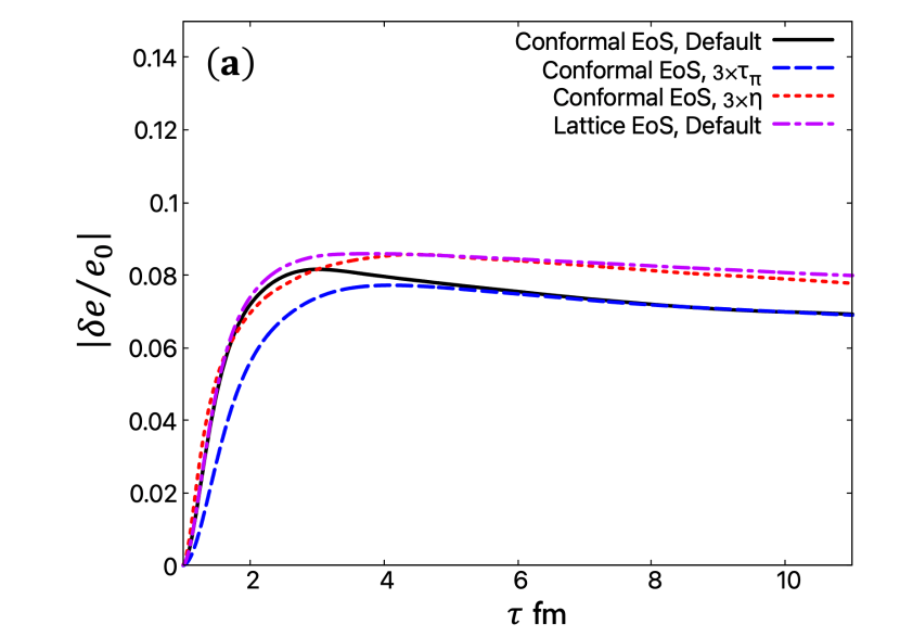
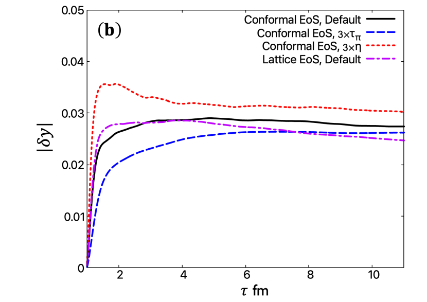
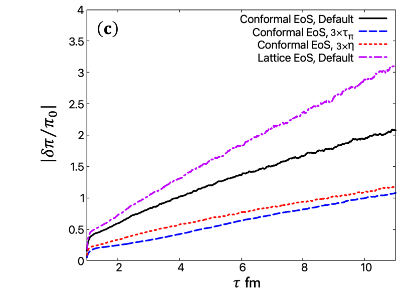
Figure 1: Absolute values of the ratio of average fluctuations and background. Time evolution of (a) energy density, (b) flow rapidity and (c) shear pressure are shown in comparison. The black solid line, blue dashed line, red dotted line and magenta dash-dotted line are results from conformal EoS with default transport coefficients, conformal EoS with three times larger $\tau_{\pi}$, conformal EoS with three times larger $\eta$, and lattice EoS with default transport coefficients, respectively. All results are averaged over 10,000 events at $\eta_{s}=5.0$.

III.2 Space-time evolution

Next, let us exhibit numerical solutions of a system of partial differential equations obtained in the previous section. At first, we describe the space-time evolution of thermodynamic variables which is a sum of the background and fluctuations. Figure 2 shows the time evolution of energy density distribution from one sampled event. It is evident that the background energy density decreases immediately from the initial value, $e_{0}(\tau=1\;\text{fm})=10\;{\rm GeV/fm^{3}}$, due to the rapid expansion of the system and that, through a system of partial differential equations, the fluctuations of energy density are induced by hydrodynamic fluctuations: Hydrodynamic fluctuations induce the fluctuations of shear pressure, $\delta\pi$, which gives a space-time rapidity dependent $pdV$ work, on the other hand, fluctuations of flow rapidity, $\delta y$, also gives a space-time dependent expansion rate of local volume, $\delta\theta$. A crucial thing is that streak like structure appears through the time evolution and is kept until the final time $\tau=11\;\text{fm}$. It means that the pattern of energy density distribution is almost frozen during the evolution and could carry the information of the early stage. One of the possible reasons of such a phenomenon is that the interplay between the diffusion of fluctuations due to the finite shear viscosity and the effect of stretching the fluctuations due to the rapid expansion of the system. That is to say, the phenomenon “freeze of distribution” is an intrinsic property of expanding system. To our best knowledge, it is shown for the first time that hydrodynamic fluctuations lead structure formation of matter created in relativistic heavy ion collisions.

In Fig. 3, the similar structure appears in the case of flow rapidity fluctuations. From Eq. (21), it is induced by the spatial gradient of fluctuations of energy density, $\delta e$, and those of shear pressure $\delta\pi$. The gradient of energy density fluctuations persists throughout the time evolution. Note that, we plotted only flow rapidity fluctuations, $\delta y$, rather than the total flow rapidity in Fig. 3 since we are interested in deviation from Bjorken’s solution (2).

Figure 4 shows the space-time evolution of shear pressure. In contrast to the case of energy density or flow rapidity, there is no such a streak like structure in the shear pressure. Shear pressure is known as “fast variables”, namely, fluctuations of shear pressure are damped very quickly since it is not a conserved variable. This is one of the main reasons why the streak like structure cannot be observed in the space-time evolution of shear pressure.

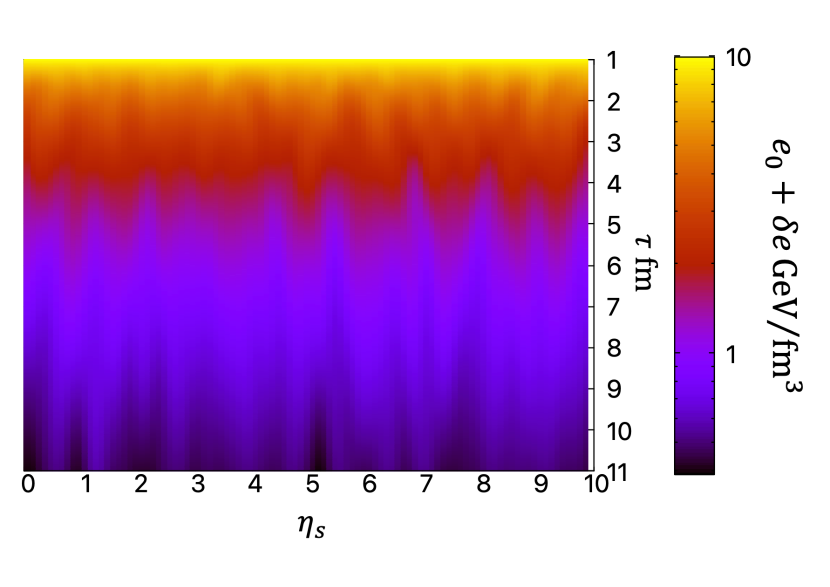
Figure 2: Space-time evolution of total energy density in an event as an example. Time passes from top to bottom and color bar indicates the magnitude of energy density.

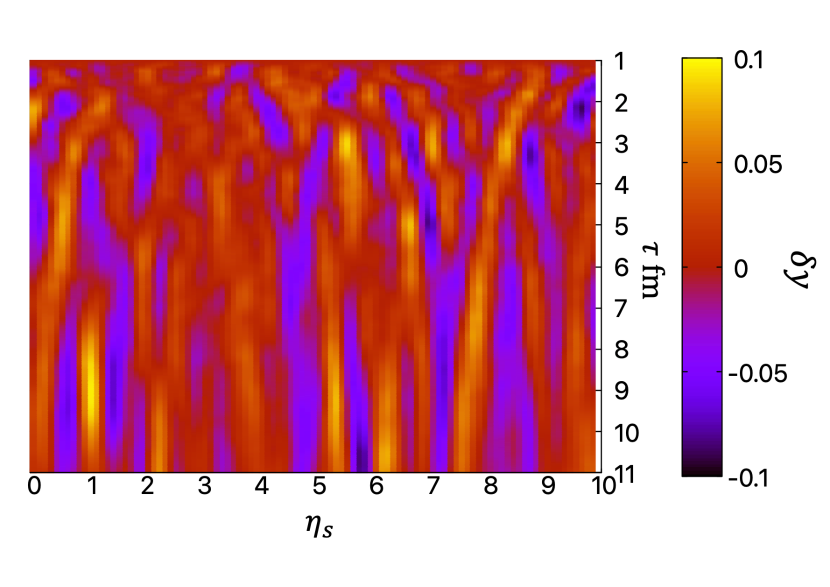
Figure 3: Space-time evolution of flow rapidity fluctuations in the same event in Fig. 2. Time passes from top to bottom and color bar indicates the magnitude of flow rapidity fluctuations.

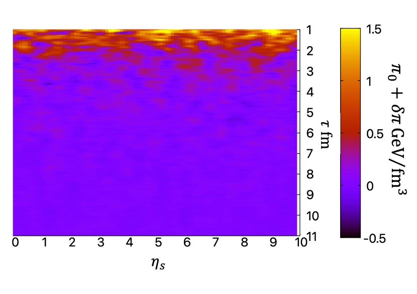
Figure 4: Space-time evolution of total shear pressure in the same event in Fig. 2. Time passes from top to bottom and color bar indicates the magnitude of shear pressure.

III.3 Correlations of fluctuations

Next, we investigate correlations of fluctuations and their dependence on various settings. Figure 5 shows the relaxation time dependence of two-point correlation functions of normalized energy density at (a) $\tau=1.5$ fm and (b) $\tau=4.0$ fm. The two-point correlation function is defined as,

$$\left<\delta\tilde{e}(\tau,\eta_{s})\delta\tilde{e}(\tau,\eta_{s}^{\prime})\right>\equiv\frac{\left<\delta e(\tau,\eta_{s})\delta e(\tau,\eta_{s}^{\prime})\right>}{e_{0}^{2}(\tau)},$$ (51)

where angular bracket $\left<\cdots\right>$ means both event average and $\eta_{s}$ average. Regarding the structure of correlations itself, correlations grow up around the origin $\Delta\eta_{s}\sim 0$ and a dip appears at $\Delta\eta_{s}\sim 0.5$. This is plausible from a viewpoint of the conservation law: the energy density at some point has a negative correlation with that in its vicinity due to energy conservation. The acausal scenario can be demonstrated by taking a $\tau_{\pi}\rightarrow 0$ limit in Eqs. (28) and (29). We obviously see a difference among the three different settings of the relaxation time at the early stage, $\tau=1.5$ fm: the correlation with smaller relaxation time of shear pressure tends to propagate faster in the space-time rapidity direction and correlation around the origin becomes stronger. However, the difference becomes tiny at the late stage, $\tau=4.0$ fm: it takes a longer time to catch up the final shape of the correlation due to a longer relaxation time. We also analyze the effect of the shear viscosity on energy density correlations in Fig. 6. Apparently, fluids with larger shear viscosity tend to behave more slowly and the dip structures are smeared.

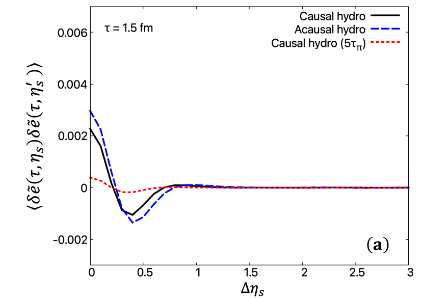
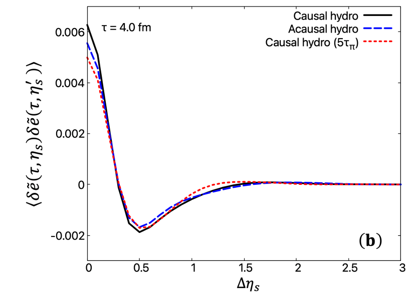
Figure 5: Normalized correlations of energy density fluctuations as functions of $\Delta\eta_{s}\equiv|\eta_{s}-\eta_{s}^{\prime}|$. We make a comparison between causal hydro (default settings, black solid line), acausal hydro ($\tau_{\pi}=0\;\text{fm}$, blue dashed line), and causal hydro ($5\tau_{\pi}$, red dotted line) at (a) $\tau=1.5\;\text{fm}$ and (b) $\tau=4.0\;\text{fm}$u.

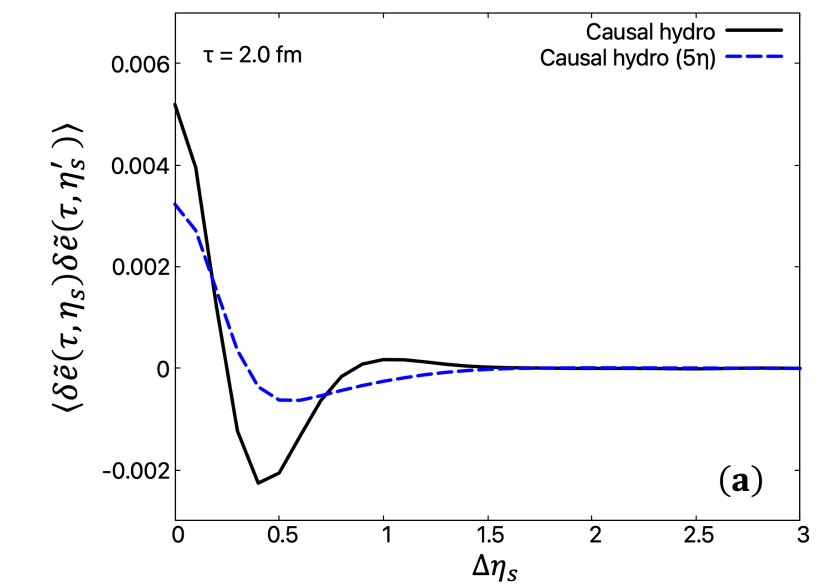
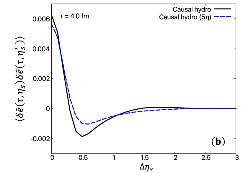
Figure 6: Normalized correlations of energy density fluctuations as functions of $\Delta\eta_{s}\equiv|\eta_{s}-\eta_{s}^{\prime}|$. We make a comparison of results from causal hydro with conformal EoS between default settings (black solid line) and 5 times larger $\eta$ (blue dashed line) at (a) $\tau=2.0\;\text{fm}$ and (b) $\tau=4.0\;\text{fm}$.

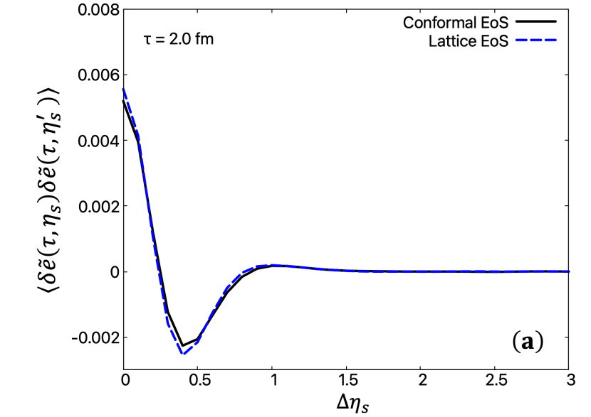
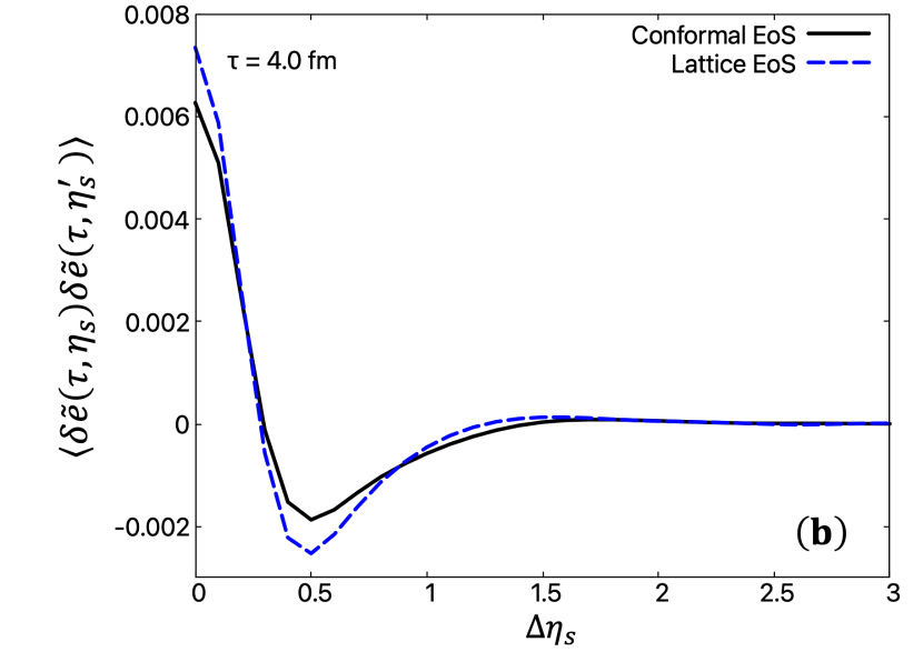
Figure 7: Normalized correlations of energy density fluctuations as functions of $\Delta\eta_{s}\equiv|\eta_{s}-\eta_{s}^{\prime}|$. We make a comparison between conformal EoS (default settings, black solid line) and lattice EoS (blue dashed line) at (a) $\tau=2.0\;\text{fm}$ and (b) $\tau=4.0\;\text{fm}$.

In Fig. 7, we make a comparison of the correlation between the conformal EoS and the lattice EoS. Although the propagation speed of information should be slightly different due to the difference of sound velocity, $c_{s}^{2}=\partial p_{0}/\partial e_{0}$, only a small difference can be seen in this comparison. In general, sound velocity of lattice EoS is smaller than that of conformal EoS. Hence, information is likely to remain around the origin at which the correlation becomes stronger. That would be the reason why we observe the difference between these two different EoS. It is noted that the difference of propagation speed can be seen in Fig. 5, which indicates relaxation time also affects the propagation in the space-time rapidity direction.

We also show correlations of flow rapidity fluctuations in Fig. 8 and shear pressure fluctuations in Fig. 9 as comparisons of the effect of model EoS. The shape of correlations of flow rapidity fluctuations is very similar to that of energy density fluctuations. It is a reasonable behavior as a variable originated from the conservation law of momentum. Note that the difference of propagation speed due to the sound velocity difference is relatively seen at $\tau=4.0\;\text{fm}$ in Fig. 8: the position of the second peaks around $\Delta\eta_{s}\sim 1$ differ. In Fig. 9, we do not observe dips and the second peaks in correlations of fluctuations of shear pressure. The difference of the shape of correlation functions comes from the property of the variable, namely, “fast variable” which is one of the diffusive quantities and is nothing to do with the conservation law unlike the “slow variables” such as energy density and flow rapidity. The correlations around the origin monotonically grow up as time evolution and the magnitude is larger in lattice EoS through the whole time evolution. It can be understood from the view point of the FDR. In fact, the shape of shear pressure correlations directly reflects the FDR since the noise term is introduced in the equation of shear pressure fluctuations (29). From the FDR (36), the magnitude of the noises is larger at higher temperature. At a fixed proper time, the background temperature under the expansion with lattice EoS is larger than that with conformal EoS since the sound velocity of the former is in general smaller than that of the latter. Thus, the magnitude of the noises is larger in lattice EoS than in conformal EoS. This behavior has already been discussed in Eq. (49) and also seen in Fig. 1 (c) in Sec. III.1.

To summarize these results, shear viscosity and relaxation time work to slow down the behaviors of correlations and also suppress the correlations around the origin and propagation in $\eta_{s}$ space. Furthermore, the model EoS also affects the behaviors of correlations, which is understood from its sound velocity difference.

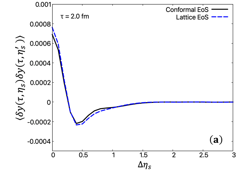
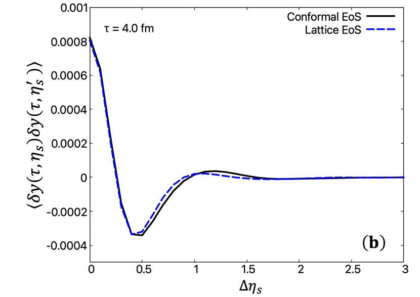
Figure 8: Correlations of flow rapidity fluctuations as functions of $\Delta\eta_{s}\equiv|\eta_{s}-\eta_{s}^{\prime}|$. We make a comparison between conformal EoS (default settings, black solid line) and lattice EoS (blue dashed line) at (a) $\tau=2.0\;\text{fm}$ and (b) $\tau=4.0\;\text{fm}$.

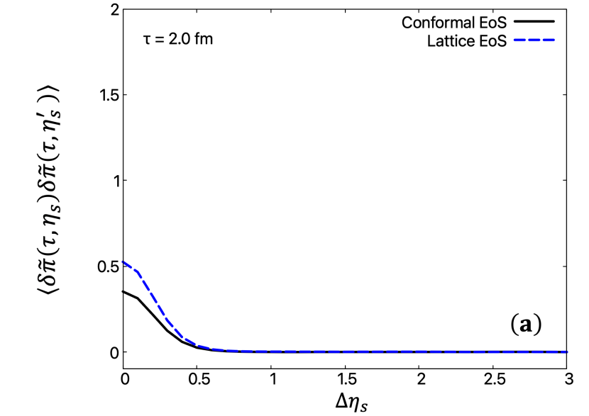
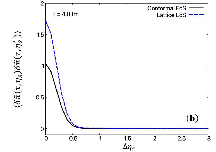
Figure 9: Normalized correlations of shear pressure fluctuations as functions of $\Delta\eta_{s}\equiv|\eta_{s}-\eta_{s}^{\prime}|$. We make a comparison between conformal EoS (default settings, black solid line) and lattice EoS (blue dashed line) at (a) $\tau=2.0\;\text{fm}$ and (b) $\tau=4.0\;\text{fm}$.

III.4 two-particle correlation functions

We have analyzed so far space-time evolution of thermodynamic variables and their correlations. We cannot, however, observe them directly in relativistic heavy ion collision experiments. Therefore it is indispensable to connect these results with experimental observables. To realize this, we calculate momentum distributions of hadrons using the Cooper-Frye formula Cooper and Frye (1974),

$$E\frac{dN}{d^{3}p}=\frac{d}{(2\pi)^{3}}\int_{\Sigma(x)}p^{\mu}d\sigma_{\mu}(x)\;f\big{(}p^{\nu}u_{\nu}(x),T(x)\big{)},$$ (52)

where, $d$, $p^{\mu}=(E,\bm{p})$, $d\sigma_{\mu}(x)$, $\Sigma(x)$, and $f(E,T)$ are degeneracy of a hadron under consideration, four-momentum, normal vector of hypersurface element, particlization hypersurface, and one-particle distribution function, respectively. Since we consider finite viscosity, viscous correction to the distribution function should be taken into account Teaney (2003); Monnai and Hirano (2009). Thus, we divide the one-particle distribution function into an equilibrium (ideal) part and a near-equilibrium (viscous) part:

$$f=f_{\rm{ideal}}+f_{\rm{vis}}.$$ (53)

For simplicity, we assume Boltzmann distribution for an equilibrium part $f_{\rm{ideal}}$ and, within our framework, it is written as

$$f_{\rm{ideal}}(p_{T},Y;\tau,\eta_{s})=\text{exp}\left[-\frac{m_{T}\cosh\left(Y-\eta_{s}-\delta y(\tau,\eta_{s})\right)}{T_{0}(\tau)+\delta T(\tau,\eta_{s})}\right],$$ (54)

where $Y\equiv\tanh^{-1}(p_{z}/E)$, $m_{T}\equiv\sqrt{p_{T}^{2}+m^{2}}$, $T_{0}$, and $\delta T$ are rapidity of particles, transverse mass, temperature of background, and fluctuation of temperature, respectively. On the other hand, a near-equilibrium part Monnai and Hirano (2009) is written as

$$f_{\rm{vis}}(p_{T},Y;\tau,\eta_{s})$$

$$=\frac{1}{2sT^{3}}f_{\rm{ideal}}p^{\mu}p^{\nu}\pi_{\mu\nu}$$

$$=\frac{1}{2(s_{0}+\delta s)(T_{0}+\delta T)^{3}}f_{\rm{ideal}}$$

$$\quad\times\left[\frac{1}{2}p_{T}^{2}-m_{T}^{2}\sinh^{2}(Y-\eta_{s}-\delta y)\right](\pi_{0}+\delta\pi),$$ (55)

where $s$ is entropy density and $s_{0}$ and $\delta s$ are its background and fluctuation, respectively. Furthermore, we consider perturbative expansion of $f_{\rm{ideal}}$ and $f_{\rm{vis}}$ with respect to the fluctuations $\delta y$, $\delta T$, $\delta s$, and $\delta\pi$ up to the first order following the same prescription as derivation of EoMs of fluctuations in Sec. II. The resultant distributions are,

$$f_{\rm{ideal}} \approx e^{-\frac{m_{T}\cosh\left(Y-\eta_{s}\right)}{T_{0}}}$$

$$+e^{-\frac{m_{T}\cosh\left(Y-\eta_{s}\right)}{T_{0}}}\left[\frac{m_{T}\sinh(Y-\eta_{s})}{T_{0}}\delta y\right.$$

$$\left.+\frac{m_{T}\cosh(Y-\eta_{s})}{T_{0}^{2}}\delta T\right]$$

$$\equiv f_{\rm{ideal},0}+\delta f_{\rm{ideal}},$$ (56)

where $f_{\rm{ideal},0}$ and $\delta f_{\rm{ideal}}$ are the zeroth and the first order perturbative term of an equilibrium part, respectively. The perturbative expansion of near-equilibrium parts leads to much more complicated form:

$$f_{\rm{vis}}\approx e^{-\frac{m_{T}\cosh\left(Y-\eta_{s}\right)}{T_{0}}}\frac{1}{2s_{0}T_{0}^{3}}\left[\frac{1}{2}p_{T}^{2}-m_{T}^{2}\sinh^{2}(Y-\eta_{s})\right]\pi_{0}$$

$$+e^{-\frac{m_{T}\cosh\left(Y-\eta_{s}\right)}{T_{0}}}\frac{1}{2s_{0}T_{0}^{3}}$$

$$\times\left\{\left[\frac{m_{T}\sinh(Y-\eta_{s})}{T_{0}}\delta y+\frac{m_{T}\cosh(Y-\eta_{s})}{T_{0}^{2}}\delta T\right]\right.$$

$$\times\left[\frac{1}{2}p_{T}^{2}-m_{T}^{2}\sinh^{2}(Y-\eta_{s})\right]\pi_{0}$$

$$-\frac{1}{T_{0}}\left(\frac{1}{c_{s}^{2}}+3\right)\left[\frac{1}{2}p_{T}^{2}-m_{T}^{2}\sinh^{2}(Y-\eta_{s})\right]\pi_{0}\delta T$$

$$+2m_{T}^{2}\sinh(Y-\eta_{s})\cosh(Y-\eta_{s})\pi_{0}\delta y$$

$$+\left.\left[\frac{1}{2}p_{T}^{2}-m_{T}^{2}\sinh^{2}(Y-\eta_{s})\right]\delta\pi\right\}$$

$$\equiv f_{\rm{vis},0}+\delta f_{\rm{vis}},$$ (57)

where $f_{\rm{vis},0}$ and $\delta f_{\rm{vis}}$ are the zeroth and the first order perturbative term of a near-equilibrium part, respectively. To summarize, we have

$$f=f_{\rm{ideal}}+f_{\rm{vis}}=f_{\rm{ideal},0}+\delta f_{\rm{ideal}}+f_{\rm{vis},0}+\delta f_{\rm{vis}}$$ (58)

as a one-particle distribution function to calculate momentum distributions via the Cooper-Frye formula (52).

Rapidity distribution of hadrons is obtained by using the relations, $d^{3}p/E=d^{2}p_{T}dY=p_{T}dp_{T}dYd\phi=m_{T}dm_{T}dYd\phi$, and by integrating over azimuthal angle:

$$\frac{dN}{dY}= \frac{d}{(2\pi)^{2}}\tau A\int_{-\infty}^{\infty}d\eta_{s}\int_{m}^{\infty}dm_{T}m_{T}^{2}\cosh(Y-\eta_{s})\;f,$$ (59)

where $A$ and $m$ are transverse area and mass of a hadron under consideration, respectively. In the above calculation, we assumed isochronous freezeout at $\tau$ and also used the relation $p^{\mu}d\sigma_{\mu}=\tau Ad\eta_{s}m_{T}\cosh(Y-\eta_{s})$ by neglecting possible small changes of freezout hypersurface due to fluctuations. By taking an average of Eq. (59) over events and integrating over $m_{T}$, the first order perturbative parts in the one-particle distribution function vanish. We finally obtain

$$\left<\frac{dN}{dY}\right>=\frac{d}{(2\pi)^{2}}\tau A\int_{Y-\Delta\eta_{s}^{\prime}}^{Y+\Delta\eta_{s}^{\prime}}d\eta_{s}\cosh{(Y-\eta_{s})}$$

$$\times e^{-\frac{m\cosh\left(Y-\eta_{s}\right)}{T_{0}}}\Biggl{\{}\left(1-\frac{1}{2s_{0}T_{0}^{3}}\frac{1}{2}m^{2}\pi_{0}\right)$$

$$\times\Biggl{[}\frac{T_{0}m^{2}}{\cosh(Y-\eta_{s})}+\frac{2T_{0}^{2}m}{\cosh^{2}(Y-\eta_{s})}+\frac{2T_{0}^{3}}{\cosh^{3}(Y-\eta_{s})}\Biggr{]}$$

$$+\frac{1}{2s_{0}T_{0}^{3}}\left(\frac{1}{2}-\sinh^{2}(Y-\eta_{s})\right)\pi_{0}$$

$$\times\Biggl{[}\frac{T_{0}m^{4}}{\cosh(Y-\eta_{s})}+\frac{4T_{0}^{2}m^{3}}{\cosh^{2}(Y-\eta_{s})}+\frac{12T_{0}^{3}m^{2}}{\cosh^{3}(Y-\eta_{s})}$$

$$+\frac{24T_{0}^{4}m}{\cosh^{4}(Y-\eta_{s})}+\frac{24T_{0}^{5}}{\cosh^{5}(Y-\eta_{s})}\Biggr{]}\Biggr{\}}.$$ (60)

Practically, we replaced the integral range of $\eta_{s}$, $[-\infty,\infty]$, with $[Y-\Delta\eta_{s}^{\prime},Y+\Delta\eta_{s}^{\prime}]$ since, for a given $Y$, a contribution from a fluid element being far away from the one at $\eta_{s}=Y$ can be negligible. We set $\Delta\eta_{s}^{\prime}=3$ in our calculations and confirmed that this range is sufficient enough to converge the integral. The first order terms, $\delta f_{\rm{ideal}}$ and $\delta f_{\rm{vis}}$, do not contribute to the final one-particle momentum distribution due to $\left<\delta f\right>=0$. It is noted that, in derivation of Eq. (III.4), an integral with respect to transverse mass is analytically solved using the incomplete Gamma function (See also Appendix B).

Two-particle correlation functions in the rapidity direction, $\left<\frac{dN}{dY_{1}}\frac{dN}{dY_{2}}\right>$, are also obtained from the Cooper-Frye formula (52) after straightforward but lengthy calculations. Here subscripts 1 and 2 are labels of particle 1 and 2, respectively. See also Appendix B for details of two-particle correlation functions. Finally, we obtain the normalized two-particle correlations $\left<\frac{dN}{dY_{1}}\frac{dN}{dY_{2}}\right>/\left<\frac{dN}{dY_{1}}\right>\left<\frac{dN}{dY_{2}}\right>$ as a function of rapidity gap $\Delta Y\equiv|Y_{1}-Y_{2}|$. In what follows, the default model of the EoS is the lattice EoS although we employ the conformal EoS for the sake of comparison.

Figure 10 shows the normalized two-particle correlation functions as functions of rapidity gap $\Delta Y$ for massless particles ($m=0$ GeV), charged pions ($m=0.139$ GeV), charged kaons ($m=0.494$ GeV), and protons ($m=0.938$ GeV) without any contributions from resonance decays. Lattice EoS and default setting for transport coefficients are employed to describe the hydrodynamic evolution in this analysis. We assume that all hadrons freeze out at $\tau=10.0\;\text{fm}$ which corresponds to freezeout temperature $T\simeq 0.168$ GeV in the lattice EoS and transport coefficients employed in this study. Since the two-particle correlation functions have a value rather than unity when two-point correlation functions such as $\langle\delta T(\eta_{s1})\delta T(\eta_{s2})\rangle$ and $\langle\delta y(\eta_{s1})\delta y(\eta_{s2})\rangle$ are finite, it is obvious that the information at freezeout is inherited by two-particle correlation functions. Moreover, the pattern of the correlations is more clearly seen for heavier hadrons. It indicates that the heavier hadrons are good probes of correlations and that they can be used to extract the properties of the expanding media. As one sees, positions and depths (heights) of dips (bumps) of correlations depend on the mass of hadrons. One can interpret this behavior from a viewpoint of thermal fluctuations. The ratio $m/T_{0}$ appeared in Eq. (III.4) is a good measure of thermal fluctuations in a fluid element and characterizes the shape of correlations: the momentum rapidity, $Y$, of heavier hadrons tends to reflect the flow rapidity, $y_{f}$, at freezeout, namely $Y\approx y_{f}$, while the pattern that correlations of thermodynamic variables possess in the space-time rapidity is blurred by thermal fluctuations in the correlations of lighter particles in momentum rapidity space.

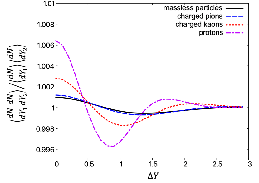
Figure 10: Normalized two-particle correlation functions as functions of $\Delta Y\equiv|Y_{1}-Y_{2}|$ for massless particles (black solid line), charged pions (blue dashed line), charged kaons (red dotted line), and protons (magenta dash-dotted line) at freezeout time $\tau=10.0\;\text{fm}$ and the corresponding background temperature $T_{0}\simeq 0.168\;\text{GeV}$. Lattice EoS is employed for hydrodynamic evolution.

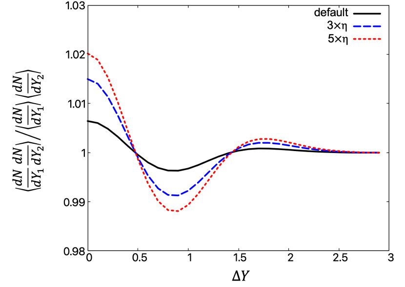
Figure 11: Normalized two-particle correlation functions of protons as functions of $\Delta Y\equiv|Y_{1}-Y_{2}|$ for default set of shear viscosity $\eta$ (black solid line), 3 times larger $\eta$ (blue dashed line), and 5 times larger $\eta$ (red dotted line) at freezeout time $\tau=10.0\;\text{fm}$. Lattice EoS and the default relaxation time are employed for hydrodynamic evolution.

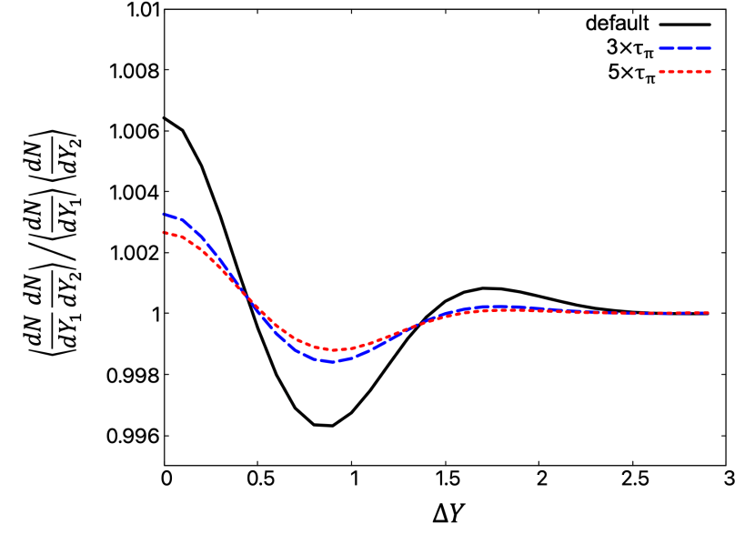
Figure 12: Normalized two-particle correlation functions of protons as functions of $\Delta Y\equiv|Y_{1}-Y_{2}|$ for default set of relaxation time $\tau_{\pi}$ (black solid line), 3 times larger $\tau_{\pi}$ (blue dashed line), and 5 times larger $\tau_{\pi}$ (red dotted line) at freezeout time $\tau=10.0\;\text{fm}$. Lattice EoS and the default shear viscosity are employed for hydrodynamic evolution.

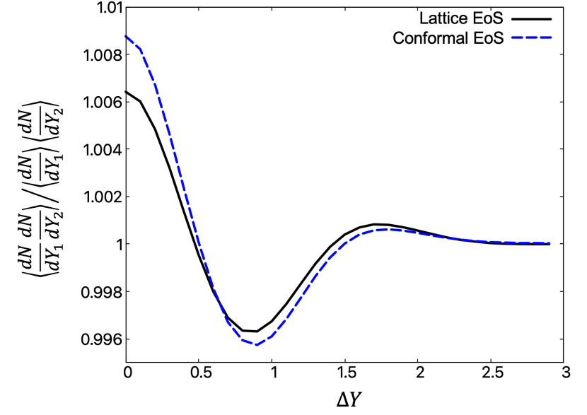
Figure 13: Normalized two-particle correlations of protons as functions of $\Delta Y\equiv|Y_{1}-Y_{2}|$. We make a comparison of the results between lattice EoS (black solid line) and conformal EoS (blue dashed line) at $T_{0}\simeq 0.168\;\text{GeV}$. Regarding the difference of freezeout time, see the text.

In Figs. 11 and 12, we elucidate how the two-particle correlation functions of protons depend on the transport coefficients under the space-time evolution with lattice EoS. The correlation pattern becomes more visible by increasing shear viscosity as shown in Fig. 11. On the other hand, the magnitude decreases with increasing relaxation time as shown in Fig. 12. The magnitude of two-particle correlation functions turns out to be highly sensitive to the transport properties of the media although positions of dips and bumps of the two-particle correlations do not depend on the choice of shear viscosity and relaxation time within a certain range. This clearly exhibits that the two-particle correlation functions of relatively heavy hadrons open up a new window to study the transport properties of the media created in relativistic heavy ion collisions.

In Fig.  13, we make a comparison of the proton two-particle correlation functions between conformal EoS and lattice EoS. When we analyze the correlation functions of energy density fluctuations, the magnitude of lattice EoS is larger than that of conformal EoS as shown in Fig. 7. However, this behavior is opposite in the two-particle correlation functions of protons: the magnitude of two particle correlation functions of protons with conformal EoS is larger than that of lattice EoS. This is due to the difference of freezeout time. In fact, fluids with conformal EoS reaches $T_{0}\simeq 0.168\;\text{GeV}$ faster than the ones with lattice EoS. Thus, freezeout time depends on the choice of the model EoS: $\tau=4.3$ fm for conformal EoS with the degree of freedom, $d=47.5$, and $\tau=10.0$ fm for lattice EoS. Thus two-particle correlation functions with conformal EoS reflect the early time correlations of thermodynamic variables which is in the course of growing up rapidly.

IV Summary

In this paper, we developed a framework which deals with causal hydrodynamic fluctuations in one-dimensional expanding system. Since the EoMs are derived without any assumption of specific constitutive equations, one employs any kinds of constitutive equations proposed so far for shear pressure $\pi$ and bulk pressure $\Pi$. In the present work, we employed the simplest second order constitutive equations derived by Israel and Stewart which satisfy the causality. We solved a system of stochastic partial differential equations and analyzed the dynamics of (1+1)-dimensional causal hydrodynamic fluctuations. Through the description of space-time evolution of thermodynamic variables, we found a novel phenomenon, an almost frozen structure of energy density fluctuations and flow rapidity fluctuations. From the analysis of the structure, it could be possible to extract the information of early stage of hydrodynamic evolution such as thermal fluctuations in the early stage. We also investigated the two-point correlation functions of energy density fluctuations which are induced by hydrodynamic fluctuations and saw the dependence on various settings of the bulk and the transport properties. The correlations are sensitive to the settings of EoS and transport coefficients such as relaxation time and viscosity. To extract properties of the media in comparison with experimental data, it is also important to analyze the effects of correlations of thermodynamic variables on two-particle correlation functions which are observables in experiment. Utilizing the Cooper-Frye formula, we analytically derived the specific form of two-particle correlation functions including two-point correlation functions of thermodynamic variables, flow rapidity, shear pressure, and cross terms among them. We show that the two-point correlations of these hydrodynamic variables are inherited by two-particle correlations in the final state. We found that correlations are more enhanced for heavier particles. It indicates that heavier hadrons are good probes to see the consequences of hydrodynamic fluctuations. We also show that the two-particle correlation functions are sensitive to the properties of the medium. Specifically, the correlations enhance with increasing shear viscosity or decreasing relaxation time. Sound velocity also affects the shape of correlations, therefore we have a chance to extract the information of EoS through analysis of the two-particle correlation functions. These results provide us with an opportunity for multidimensional analysis of properties of the QGP created in the relativistic heavy ion collisions.

In the present paper, we assumed one of the simplest settings, e.g., the simplest one-dimensional expanding system, the simplest EoS, the simplest constitutive equations, and neglect of charge current and bulk pressure. Therefore, there are a lot of room for sophistication and extension. As one way of big extension, the (3+1)-dimensional expanding analytic solution Gubser (2010), instead of one-dimensional boost invariant solution (2), could be employed by following the same prescription as we explained in this paper. Regarding the FDRs (33) and (35), it is known that these FDRs need additional correction terms when the background system is non-static and constitute equations have finite relaxation effects Murase (2019). It would be intriguing to see the effects of expansion and finite relaxation on the two-point correlations of hydrodynamic variables.

The present framework can be utilized to search for the critical point of the QCD phase diagram through the analysis of detailed dynamics of both hydrodynamic and critical fluctuations. Fluctuations of the order parameter of chiral phase transition in vicinity of the critical point are “fast modes”, therefore such information is likely to be lost due to the diffusive mode in the QGP. The fluctuations of the order parameter are, however, taken over by the “slow modes”, namely, fluctuations of baryon number density Fujii and Ohtani (2004); Son and Stephanov (2004). Chasing the dynamics of both the slow modes and the fast mode Sakai et al. (2023), we can diagnose the QCD phase diagram and have a chance to pin down the location of the critical point, but leave it for the future study.

Appendix A Sound propagation

Here, let us discuss the propagation of sound wave (or density fluctuations) in $t$-$z$ plane and $\tau$-$\eta_{s}$ plane and show that the behavior is completely different if the background medium expands. To demonstrate this, we assume the sound velocity of the media is $c_{s}=1/\sqrt{3}$. One can define the effective sound velocity, in which the tailwind from the expanding system is included, as

$$c_{s}^{\prime}(t,z)=\frac{dz}{dt}=\tanh\left(\eta_{s}(t,z)+y_{s}\right)=\frac{c_{s}t+z}{t+c_{s}z},$$ (61)

where $\eta_{s}(t,z)=\tanh^{-1}(z/t)$ and $y_{s}\equiv\tanh^{-1}c_{s}\simeq 0.66$. We solve Eq. (61) with an initial condition, $z(t=1\;\mathrm{fm})=0$ numerically and transform the solution to $\tau=\sqrt{t^{2}-z^{2}}$ and $\eta_{s}=\frac{1}{2}\ln[(t+z)/(t-z))]$ when needed. Figure 14 shows the resultant propagation of sounds in $t$-$z$ plane and $\tau$-$\eta_{s}$ plane. Propagation of light is described as either $t=z+1$ in $t$-$z$ plane or $\tau=e^{\eta_{s}}$ in $\tau$-$\eta_{s}$ plane. In contrast to the case without tailwind, the slope of the propagation with tailwind approaches that of light cone asymptotically in $t$-$z$ plane. In other words, propagation speed of sound approaches the speed of light in the long time limit even though the initial sound velocity is $c_{s}=1/\sqrt{3}$ due to the expansion of the system. Moreover, propagation of sounds goes to infinity in $\eta_{s}$ space in this case. On the other hand, there is a singularity at $\eta_{s}=\tanh^{-1}(1/\sqrt{3})\simeq 0.66$ in $\tau$-$\eta_{s}$ plane in the case without tailwind. This is the so-called “sound horizon”.

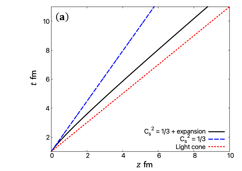
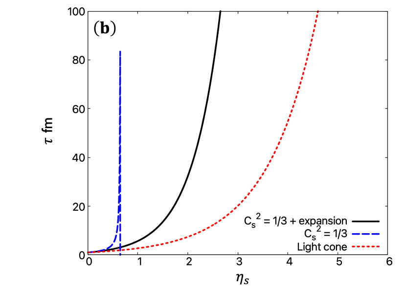
Figure 14: Sound propagation in (a) $t-z$ plane and in (b) $\tau-\eta_{s}$ plane. The black solid line, blue dashed line, and red dotted line denote propagation with tailwind, that without tailwind, and light cone, respectively. Sound velocity $c_{s}=1/\sqrt{3}$ is assumed.

Appendix B Two-particle correlation functions

We obtain the event-averaged two-particle correlation function as a function of rapidity gap after inserting the explicit forms of distribution functions (56) and (57) into the following form:

$$\left<\frac{dN}{dY_{1}}\frac{dN}{dY_{2}}\right>$$

$$=\left[\frac{d\tau A}{(2\pi)^{2}}\right]^{2}\int_{Y_{1}-\Delta\eta_{s1}^{\prime}}^{Y_{1}+\Delta\eta_{s1}^{\prime}}d\eta_{s1}\int_{Y_{2}-\Delta\eta_{s2}^{\prime}}^{Y_{2}+\Delta\eta_{s2}^{\prime}}d\eta_{s2}$$

$$\times\int_{m}^{\infty}dm_{T1}\int_{m}^{\infty}dm_{T2}m_{T1}^{2}m_{T2}^{2}\cosh(Y_{1}-\eta_{s1})\cosh(Y_{2}-\eta_{s2})$$

$$\times\left<\left(f_{\rm{ideal,0}}^{(1)}f_{\rm{ideal,0}}^{(2)}+2f_{\rm{ideal,0}}^{(1)}f_{\rm{vis,0}}^{(2)}+f_{\rm{vis,0}}^{(1)}f_{\rm{vis,0}}^{(2)}\right.\right.$$

$$\left.\left.+\delta f_{\rm{ideal}}^{(1)}\delta f_{\rm{ideal}}^{(2)}+2\delta f_{\rm{ideal}}^{(1)}\delta f_{\rm{vis}}^{(2)}+\delta f_{\rm{vis}}^{(1)}\delta f_{\rm{vis}}^{(2)}\right)\right>.$$ (62)

Here upper indices 1 and 2 in the distribution functions denote variables of particle 1 and 2, respectively. Terms including single $\delta f_{\rm{ideal}}$ or $\delta f_{\rm{vis}}$ are neglected since they do not contribute to the final results due to $\left<\delta f\right>=0$. The next step is to integrate Eq. (B) over $m_{T1}$ and $m_{T2}$. Since the resultant form of two-particle correlation functions is significantly complicated, we introduce new variables as follows to avoid the complexity:

$$A_{1/2}(n) \equiv\sum_{i=0}^{n}\frac{T_{0}^{i+1}P(n,i)m_{T1/2}^{n-i}}{\cosh^{i+1}(Y_{1/2}-\eta_{s1/2})},$$ (63)

$$B \equiv\frac{1}{2s_{0}T_{0}^{3}},$$ (64)

$$C_{1/2} \equiv\frac{1}{2}-\sinh^{2}(Y_{1/2}-\eta_{s1/2}),$$ (65)

$$D \equiv\frac{1}{2}m^{2},$$ (66)

$$E \equiv\frac{1}{2s_{0}T_{0}}\left(\frac{1}{c_{s}^{2}}+3\right),$$ (67)

$$F_{1/2} \equiv 2\sinh(Y_{1/2}-\eta_{s1/2})\cosh(Y_{1/2}-\eta_{s1/2}),$$ (68)

$$G_{12} \equiv\frac{\cosh(Y_{1}-\eta_{s1})\cosh(Y_{2}-\eta_{s2})}{T_{0}^{4}}\delta T(\eta_{s1})\delta T(\eta_{s2})$$

$$+\frac{\sinh(Y_{1}-\eta_{s1})\cosh(Y_{2}-\eta_{s2})}{T_{0}^{3}}\delta y(\eta_{s1})\delta T(\eta_{s2})$$

$$+\frac{\cosh(Y_{1}-\eta_{s1})\sinh(Y_{2}-\eta_{s2})}{T_{0}^{3}}\delta T(\eta_{s1})\delta y(\eta_{s2})$$

$$+\frac{\sinh(Y_{1}-\eta_{s1})\sinh(Y_{2}-\eta_{s2})}{T_{0}^{2}}\delta y(\eta_{s1})\delta y(\eta_{s2}).$$ (69)

Here the index “$1/2$” denotes either particle 1 or particle 2. A coefficient of incomplete Gamma function, $A_{1/2}(n)$, is defined as

$$\int_{m}^{\infty}dm_{T1/2}m_{T1/2}^{n}e^{-\frac{m_{T1/2}\cosh(Y_{1/2}-\eta_{s1/2})}{T_{0}}}$$

$$=\sum_{i=0}^{n}\frac{T_{0}^{i+1}P(n,i)m_{T1/2}^{n-i}}{\cosh^{i+1}(Y_{1/2}-\eta_{s1/2})}e^{-\frac{m\cosh(Y_{1/2}-\eta_{s1/2})}{T_{0}}}$$

$$=A_{1/2}(n)e^{-\frac{m\cosh(Y_{1/2}-\eta_{s1/2})}{T_{0}}},$$ (70)

where the permutation is calculated as $P(n,i)=n!/(n-i)!$. Using these variables, the resultant two-particle correlation is lead to

$$\left<\frac{dN}{dY_{1}}\frac{dN}{dY_{2}}\right>$$

$$=\left[\frac{d\tau A}{(2\pi)^{2}}\right]^{2}\int_{Y_{1}-\Delta\eta_{s1}^{\prime}}^{Y_{1}+\Delta\eta_{s1}^{\prime}}d\eta_{s1}\int_{Y_{2}-\Delta\eta_{s2}^{\prime}}^{Y_{2}+\Delta\eta_{s2}^{\prime}}d\eta_{s2}$$

$$\times\cosh(Y_{1}-\eta_{s1})\cosh(Y_{2}-\eta_{s2})$$

$$\times\left<\left(\mathrm{(I)}+2\times\mathrm{(II)}+\mathrm{(III)}+\mathrm{(IV)}+2\times\mathrm{(V)}+\mathrm{(VI)}\right)\right>,$$ (71)

$$\mathrm{(I)} =\int_{m}^{\infty}dm_{T1}\int_{m}^{\infty}dm_{T2}m_{T1}^{2}m_{T2}^{2}f_{\rm{ideal,0}}^{(1)}f_{\rm{ideal,0}}^{(2)}$$

$$=A_{1}(2)A_{2}(2)e^{-\frac{m\left[\cosh(Y_{1}-\eta_{s1})+\cosh(Y_{2}-\eta_{s2})\right]}{T_{0}}},$$ (72)

$$\mathrm{(II)} =\int_{m}^{\infty}dm_{T1}\int_{m}^{\infty}dm_{T2}m_{T1}^{2}m_{T2}^{2}f_{\rm{ideal,0}}^{(1)}f_{\rm{vis,0}}^{(2)}$$

$$=\big{[}A_{1}(2)A_{2}(4)BC_{2}\pi_{0}-A_{1}(2)A_{2}(2)BD\pi_{0}\big{]}$$

$$\times e^{-\frac{m\left[\cosh(Y_{1}-\eta_{s1})+\cosh(Y_{2}-\eta_{s2})\right]}{T_{0}}},$$ (73)

$$\mathrm{(III)} =\int_{m}^{\infty}dm_{T1}\int_{m}^{\infty}dm_{T2}m_{T1}^{2}m_{T2}^{2}f_{\rm{vis,0}}^{(1)}f_{\rm{vis,0}}^{(2)}$$

$$=\big{[}A_{1}(4)A_{2}(4)B^{2}C_{1}C_{2}\pi_{0}^{2}-A_{1}(4)A_{2}(2)B^{2}C_{1}D\pi_{0}^{2}$$

$$-A_{1}(2)A_{2}(4)B^{2}C_{2}D\pi_{0}^{2}+A_{1}(2)A_{2}(2)B^{2}D^{2}\pi_{0}^{2}\big{]}$$

$$\times e^{-\frac{m\left[\cosh(Y_{1}-\eta_{s1})+\cosh(Y_{2}-\eta_{s2})\right]}{T_{0}}},$$ (74)

$$\mathrm{(IV)} =\int_{m}^{\infty}dm_{T1}\int_{m}^{\infty}dm_{T2}m_{T1}^{2}m_{T2}^{2}\delta f_{\rm{ideal}}^{(1)}\delta f_{\rm{ideal}}^{(2)}$$

$$=A_{1}(3)A_{2}(3)G_{12}e^{-\frac{m\left[\cosh(Y_{1}-\eta_{s1})+\cosh(Y_{2}-\eta_{s2})\right]}{T_{0}}},$$ (75)

$$\mathrm{(V)} =\int_{m}^{\infty}dm_{T1}\int_{m}^{\infty}dm_{T2}m_{T1}^{2}m_{T2}^{2}\delta f_{\rm{ideal}}^{(1)}\delta f_{\rm{vis}}^{(2)}$$

$$=\Bigg{\{}A_{1}(3)A_{2}(5)G_{12}BC_{2}\pi_{0}-A_{1}(3)A_{2}(3)G_{12}BD\pi_{0}$$

$$-A_{1}(3)A_{2}(4)EC_{2}\pi_{0}$$

$$\times\Big{[}\frac{\sinh(Y_{1}-\eta_{s1})}{T_{0}}\delta y(\eta_{s1})\delta T(\eta_{s2})$$

$$+\frac{\cosh(Y_{1}-\eta_{s1})}{T_{0}^{2}}\delta T(\eta_{s1})\delta T(\eta_{s2})\Big{]}$$

$$+A_{1}(3)A_{2}(4)BF_{2}\pi_{0}$$

$$\times\Big{[}\frac{\sinh(Y_{1}-\eta_{s1})}{T_{0}}\delta y(\eta_{s1})\delta y(\eta_{s2})$$

$$+\frac{\cosh(Y_{1}-\eta_{s1})}{T_{0}^{2}}\delta T(\eta_{s1})\delta y(\eta_{s2})\Big{]}$$

$$+A_{1}(3)A_{2}(4)BC_{2}$$

$$\times\Big{[}\frac{\sinh(Y_{1}-\eta_{s1})}{T_{0}}\delta y(\eta_{s1})\delta\pi(\eta_{s2})$$

$$+\frac{\cosh(Y_{1}-\eta_{s1})}{T_{0}^{2}}\delta T(\eta_{s1})\delta\pi(\eta_{s2})\Big{]}$$

$$+A_{1}(3)A_{2}(2)ED\pi_{0}$$

$$\times\Big{[}\frac{\sinh(Y_{1}-\eta_{s1})}{T_{0}}\delta y(\eta_{s1})\delta T(\eta_{s2})$$

$$+\frac{\cosh(Y_{1}-\eta_{s1})}{T_{0}^{2}}\delta T(\eta_{s1})\delta T(\eta_{s2})\Big{]}$$

$$-A_{1}(3)A_{2}(2)BD$$

$$\times\Big{[}\frac{\sinh(Y_{1}-\eta_{s1})}{T_{0}}\delta y(\eta_{s1})\delta\pi(\eta_{s2})$$

$$+\frac{\cosh(Y_{1}-\eta_{s1})}{T_{0}^{2}}\delta T(\eta_{s1})\delta\pi(\eta_{s2})\Big{]}\Bigg{\}}$$

$$\times e^{-\frac{m\left[\cosh(Y_{1}-\eta_{s1})+\cosh(Y_{2}-\eta_{s2})\right]}{T_{0}}},$$ (76)

$$\mathrm{(VI)} =\int_{m}^{\infty}dm_{T1}\int_{m}^{\infty}dm_{T2}m_{T1}^{2}m_{T2}^{2}\delta f_{\rm{vis}}^{(1)}\delta f_{\rm{vis}}^{(2)}$$

$$=\Bigg{(}\Big{\{}A_{1}(5)A_{2}(5)G_{12}B^{2}C_{1}C_{2}\pi_{0}^{2}-A_{1}(5)A_{2}(3)G_{12}B^{2}C_{1}D\pi_{0}^{2}$$

$$-A_{1}(3)A_{2}(5)G_{12}B^{2}C_{2}D\pi_{0}^{2}+A_{1}(3)A_{2}(3)G_{12}B^{2}D^{2}\pi_{0}^{2}$$

$$+\Big{[}A_{1}(4)A_{2}(4)E^{2}C_{1}C_{2}\pi_{0}^{2}-A_{1}(4)A_{2}(2)E^{2}C_{1}D\pi_{0}^{2}$$

$$-A_{1}(2)A_{2}(4)E^{2}C_{2}D\pi_{0}^{2}+A_{1}(2)A_{2}(2)E^{2}D^{2}\pi_{0}^{2}\Big{]}$$

$$\times\delta T(\eta_{s1})\delta T(\eta_{s2})$$

$$+A_{1}(4)A_{2}(4)B^{2}F_{1}F_{2}\pi_{0}^{2}\delta y(\eta_{s1})\delta y(\eta_{s2})$$

$$+\Big{[}A_{1}(4)A_{2}(4)B^{2}C_{1}C_{2}-A_{1}(4)A_{2}(2)B^{2}C_{1}D$$

$$-A_{1}(2)A_{2}(4)B^{2}C_{2}D+A_{1}(2)A_{2}(2)B^{2}D^{2}\Big{]}$$

$$\times\delta\pi(\eta_{s1})\delta\pi(\eta_{s2})\Big{\}}$$

$$+2\Big{\{}\Big{[}-A_{1}(5)A_{2}(4)BEC_{1}C_{2}\pi_{0}^{2}+A_{1}(3)A_{2}(4)BEDC_{2}\pi_{0}^{2}$$

$$+A_{1}(5)A_{2}(2)BEC_{1}D\pi_{0}^{2}-A_{1}(3)A_{2}(2)BED^{2}\pi_{0}^{2}\Big{]}$$

$$\times\Big{[}\frac{\sinh(Y_{1}-\eta_{s1})}{T_{0}}\delta y(\eta_{s1})\delta T(\eta_{s2})$$

$$+\frac{\cosh(Y_{1}-\eta_{s1})}{T_{0}^{2}}\delta T(\eta_{s1})\delta T(\eta_{s2})\Big{]}$$

$$+\Big{[}A_{1}(5)A_{2}(4)B^{2}C_{1}F_{2}\pi_{0}^{2}-A_{1}(3)A_{2}(4)B^{2}DF_{2}\pi_{0}^{2}\Big{]}$$

$$\times\Big{[}\frac{\sinh(Y_{1}-\eta_{s1})}{T_{0}}\delta y(\eta_{s1})\delta y(\eta_{s2})$$

$$+\frac{\cosh(Y_{1}-\eta_{s1})}{T_{0}^{2}}\delta T(\eta_{s1})\delta y(\eta_{s2})\Big{]}$$

$$+\Big{[}A_{1}(5)A_{2}(4)B^{2}C_{1}C_{2}\pi_{0}-A_{1}(3)A_{2}(4)B^{2}DC_{2}\pi_{0}$$

$$-A_{1}(5)A_{2}(2)B^{2}C_{1}D\pi_{0}+A_{1}(3)A_{2}(2)B^{2}D^{2}\pi_{0}\Big{]}$$

$$\times\Big{[}\frac{\sinh(Y_{1}-\eta_{s1})}{T_{0}}\delta y(\eta_{s1})\delta\pi(\eta_{s2})$$

$$+\frac{\cosh(Y_{1}-\eta_{s1})}{T_{0}^{2}}\delta T(\eta_{s1})\delta\pi(\eta_{s2})\Big{]}$$

$$+\Big{[}-A_{1}(4)A_{2}(4)BEC_{1}F_{2}\pi_{0}^{2}+A_{1}(2)A_{2}(4)BEDF_{2}\pi_{0}^{2}\Big{]}$$

$$\times\delta T(\eta_{s1})\delta y(\eta_{s2})$$

$$+\Big{[}-A_{1}(4)A_{2}(4)BEC_{1}C_{2}\pi_{0}+A_{1}(4)A_{2}(2)BEC_{1}D\pi_{0}$$

$$+A_{1}(2)A_{2}(4)BEC_{2}D\pi_{0}-A_{1}(2)A_{2}(2)BED^{2}\pi_{0}\Big{]}$$

$$\times\delta T(\eta_{s1})\delta\pi(\eta_{s2})$$

$$+\Big{[}A_{1}(4)A_{2}(4)B^{2}F_{1}C_{2}\pi_{0}-A_{1}(4)A_{2}(2)B^{2}F_{1}D\pi_{0}\Big{]}$$

$$\times\delta y(\eta_{s1})\delta\pi(\eta_{s2})\Big{\}}\Bigg{)}$$

$$\times e^{-\frac{m\left[\cosh(Y_{1}-\eta_{s1})+\cosh(Y_{2}-\eta_{s2})\right]}{T_{0}}}.$$ (77)

The terms (IV), (V), and (VI) play a crucial role in reflecting the correlations of thermodynamic variables in the two-particle correlation functions. Performing $\eta_{s1}$ and $\eta_{s2}$ integration of (B) numerically, we finally obtain the two-particle correlation as a function of rapidity gap, $\Delta Y\equiv|Y_{1}-Y_{2}|$.

In Eq. (B), we considered up to the second order in perturbation (fluctuation) and up to the second order in viscous correction. Orders of each term are summarized in Table 2.

Table 2: Orders of each term

Term	Perturbation	Viscous correction
$f_{\rm{ideal,0}}f_{\rm{ideal,0}}$	0	0
$f_{\rm{ideal,0}}f_{\rm{vis,0}}$	0	1
$f_{\rm{vis,0}}f_{\rm{vis,0}}$	0	2
$\delta f_{\rm{ideal}}\delta f_{\rm{ideal}}$	2	0
$\delta f_{\rm{ideal}}\delta f_{\rm{vis}}$	2	1
$\delta f_{\rm{vis}}\delta f_{\rm{vis}}$	2	2

Strictly speaking, the second order perturbative terms from the one-particle distribution or the second order viscous corrections should have been considered from an order counting point of view in the form of two-particle correlation (B), e.g., $f_{\rm{ideal,0}}\delta^{2}f_{\rm{vis}}$. However, we neglected such terms since we expanded the distribution only up to the first order of perturbation and viscous correction as Eq. (58).

References

- Kolb et al. (2001) P. F. Kolb, P. Huovinen, U. W. Heinz, and H. Heiselberg, Phys. Lett. B 500, 232 (2001), arXiv:hep-ph/0012137 .
- Huovinen et al. (2001) P. Huovinen, P. F. Kolb, U. W. Heinz, P. V. Ruuskanen, and S. A. Voloshin, Phys. Lett. B 503, 58 (2001), arXiv:hep-ph/0101136 .
- Heinz and Kolb (2002) U. W. Heinz and P. F. Kolb, Nucl. Phys. A 702, 269 (2002), arXiv:hep-ph/0111075 .
- Teaney et al. (2001) D. Teaney, J. Lauret, and E. V. Shuryak, Phys. Rev. Lett. 86, 4783 (2001), arXiv:nucl-th/0011058 .
- Hirano (2002) T. Hirano, Phys. Rev. C 65, 011901 (2002), arXiv:nucl-th/0108004 .
- Hirano and Tsuda (2002) T. Hirano and K. Tsuda, Phys. Rev. C 66, 054905 (2002), arXiv:nucl-th/0205043 .
- Hirano and Gyulassy (2006) T. Hirano and M. Gyulassy, Nucl. Phys. A 769, 71 (2006), arXiv:nucl-th/0506049 .
- Bernhard et al. (2016) J. E. Bernhard, J. S. Moreland, S. A. Bass, J. Liu, and U. Heinz, Phys. Rev. C 94, 024907 (2016), arXiv:1605.03954 [nucl-th] .
- Bernhard et al. (2019) J. E. Bernhard, J. S. Moreland, and S. A. Bass, Nature Phys. 15, 1113 (2019).
- Auvinen et al. (2020) J. Auvinen, K. J. Eskola, P. Huovinen, H. Niemi, R. Paatelainen, and P. Petreczky, Phys. Rev. C 102, 044911 (2020), arXiv:2006.12499 [nucl-th] .
- Nijs et al. (2021a) G. Nijs, W. van der Schee, U. Gürsoy, and R. Snellings, Phys. Rev. Lett. 126, 202301 (2021a), arXiv:2010.15130 [nucl-th] .
- Nijs et al. (2021b) G. Nijs, W. van der Schee, U. Gürsoy, and R. Snellings, Phys. Rev. C 103, 054909 (2021b), arXiv:2010.15134 [nucl-th] .
- Parkkila et al. (2021) J. E. Parkkila, A. Onnerstad, and D. J. Kim, Phys. Rev. C 104, 054904 (2021), arXiv:2106.05019 [hep-ph] .
- Everett et al. (2021) D. Everett et al. (JETSCAPE), Phys. Rev. C 103, 054904 (2021), arXiv:2011.01430 [hep-ph] .
- Kubo (1957) R. Kubo, J. Phys. Soc. Jap. 12, 570 (1957).
- Bjorken (1983) J. D. Bjorken, Phys. Rev. D 27, 140 (1983).
- Kouno et al. (1990) H. Kouno, M. Maruyama, F. Takagi, and K. Saito, Phys. Rev. D 41, 2903 (1990).
- Denicol et al. (2008) G. S. Denicol, T. Kodama, T. Koide, and P. Mota, J. Phys. G 35, 115102 (2008), arXiv:0807.3120 [hep-ph] .
- Kapusta et al. (2012) J. I. Kapusta, B. Muller, and M. Stephanov, Phys. Rev. C 85, 054906 (2012), arXiv:1112.6405 [nucl-th] .
- Yan and Grönqvist (2016) L. Yan and H. Grönqvist, JHEP 03, 121 (2016), arXiv:1511.07198 [nucl-th] .
- Gubser (2010) S. S. Gubser, Phys. Rev. D 82, 085027 (2010), arXiv:1006.0006 [hep-th] .
- Hiscock and Lindblom (1983) W. A. Hiscock and L. Lindblom, Annals Phys. 151, 466 (1983).
- Hiscock and Lindblom (1985) W. A. Hiscock and L. Lindblom, Phys. Rev. D 31, 725 (1985).
- Hiscock and Lindblom (1987) W. A. Hiscock and L. Lindblom, Phys. Rev. D 35, 3723 (1987).
- Israel (1976) W. Israel, Annals Phys. 100, 310 (1976).
- Israel and Stewart (1979) W. Israel and J. M. Stewart, Annals Phys. 118, 341 (1979).
- Baier et al. (2006) R. Baier, P. Romatschke, and U. A. Wiedemann, Phys. Rev. C 73, 064903 (2006), arXiv:hep-ph/0602249 .
- Baier et al. (2008) R. Baier, P. Romatschke, D. T. Son, A. O. Starinets, and M. A. Stephanov, JHEP 04, 100 (2008), arXiv:0712.2451 [hep-th] .
- Betz et al. (2009a) B. Betz, D. Henkel, and D. H. Rischke, Prog. Part. Nucl. Phys. 62, 556 (2009a), arXiv:0812.1440 [nucl-th] .
- Betz et al. (2009b) B. Betz, D. Henkel, and D. H. Rischke, J. Phys. G 36, 064029 (2009b).
- Denicol et al. (2012) G. S. Denicol, H. Niemi, E. Molnar, and D. H. Rischke, Phys. Rev. D 85, 114047 (2012), [Erratum: Phys.Rev.D 91, 039902 (2015)], arXiv:1202.4551 [nucl-th] .
- Monnai and Hirano (2010) A. Monnai and T. Hirano, Nucl. Phys. A 847, 283 (2010), arXiv:1003.3087 [nucl-th] .
- Jaiswal et al. (2013) A. Jaiswal, R. S. Bhalerao, and S. Pal, Phys. Rev. C 87, 021901 (2013), arXiv:1302.0666 [nucl-th] .
- Jaiswal (2013) A. Jaiswal, Phys. Rev. C 87, 051901 (2013), arXiv:1302.6311 [nucl-th] .
- Tsumura et al. (2015) K. Tsumura, Y. Kikuchi, and T. Kunihiro, Phys. Rev. D 92, 085048 (2015), arXiv:1506.00846 [hep-ph] .
- Young (2014) C. Young, Phys. Rev. C 89, 024913 (2014), arXiv:1306.0472 [nucl-th] .
- Murase and Hirano (2013) K. Murase and T. Hirano, (2013), arXiv:1304.3243 [nucl-th] .
- Murase (2015) K. Murase, Causal hydrodynamic fluctuations and their effects on high-energy nuclear collisions, Ph.D. thesis, Tokyo U. (2015).
- Murase and Hirano (2016) K. Murase and T. Hirano, Nucl. Phys. A 956, 276 (2016), arXiv:1601.02260 [nucl-th] .
- Singh (2021) M. Singh, Characterizing the quark gluon plasma using soft thermal fluctuations and hard parton interactions, Ph.D. thesis, McGill U. (2021).
- Sakai et al. (2020) A. Sakai, K. Murase, and T. Hirano, Phys. Rev. C 102, 064903 (2020), arXiv:2003.13496 [nucl-th] .
- Sakai et al. (2022) A. Sakai, K. Murase, and T. Hirano, Phys. Lett. B 829, 137053 (2022), arXiv:2111.08963 [nucl-th] .
- Kuroki et al. (2023) K. Kuroki, A. Sakai, K. Murase, and T. Hirano, Phys. Lett. B 842, 137958 (2023), arXiv:2305.01977 [nucl-th] .
- Murase (2019) K. Murase, Annals Phys. 411, 167969 (2019), arXiv:1904.11217 [nucl-th] .
- Hirano et al. (2019) T. Hirano, R. Kurita, and K. Murase, Nucl. Phys. A 984, 44 (2019), arXiv:1809.04773 [nucl-th] .
- Kloeden and Platen (1992) P. E. Kloeden and E. Platen, Numerical Solution of Stochastic Differential Equations (Springer Berlin, Heidelberg, 1992).
- Bazavov et al. (2014) A. Bazavov et al. (HotQCD), Phys. Rev. D 90, 094503 (2014), arXiv:1407.6387 [hep-lat] .
- Kovtun et al. (2005) P. Kovtun, D. T. Son, and A. O. Starinets, Phys. Rev. Lett. 94, 111601 (2005), arXiv:hep-th/0405231 .
- Cooper and Frye (1974) F. Cooper and G. Frye, Phys. Rev. D 10, 186 (1974).
- Teaney (2003) D. Teaney, Phys. Rev. C 68, 034913 (2003), arXiv:nucl-th/0301099 .
- Monnai and Hirano (2009) A. Monnai and T. Hirano, Phys. Rev. C 80, 054906 (2009), arXiv:0903.4436 [nucl-th] .
- Fujii and Ohtani (2004) H. Fujii and M. Ohtani, Phys. Rev. D 70, 014016 (2004), arXiv:hep-ph/0402263 .
- Son and Stephanov (2004) D. T. Son and M. A. Stephanov, Phys. Rev. D 70, 056001 (2004), arXiv:hep-ph/0401052 .
- Sakai et al. (2023) A. Sakai, K. Murase, H. Fujii, and T. Hirano, Acta Phys. Polon. Supp. 16, 1 (2023).