A Quasi-Wasserstein Loss for Learning Graph Neural Networks

Abstract

When learning graph neural networks (GNNs) in node-level prediction tasks, most existing loss functions are applied for each node independently, even if node embeddings and their labels are non-i.i.d. because of their graph structures. To eliminate such inconsistency, in this study we propose a novel Quasi-Wasserstein (QW) loss with the help of the optimal transport defined on graphs, leading to new learning and prediction paradigms of GNNs. In particular, we design a “Quasi-Wasserstein” distance between the observed multi-dimensional node labels and their estimations, optimizing the label transport defined on graph edges. The estimations are parameterized by a GNN in which the optimal label transport may determine the graph edge weights optionally. By reformulating the strict constraint of the label transport to a Bregman divergence-based regularizer, we obtain the proposed Quasi-Wasserstein loss associated with two efficient solvers learning the GNN together with optimal label transport. When predicting node labels, our model combines the output of the GNN with the residual component provided by the optimal label transport, leading to a new transductive prediction paradigm. Experiments show that the proposed QW loss applies to various GNNs and helps to improve their performance in node-level classification and regression tasks.

1 Introduction

Graph neural network (GNN) plays a central role in many graph learning tasks, such as social network analysis Qiu et al. 2018, Fan et al. 2019, Zhang et al. 2023, molecular modeling Satorras et al. 2021, Jiang et al. 2021, Wang et al. 2022, transportation forecasting Wang et al. 2020, Li and Zhu 2021, and so on. Given a graph with node features, a GNN embeds the graph nodes by exchanging and aggregating the node features, whose implementation is based on message-passing operators in the spatial domain Niepert et al. 2016, Kipf and Welling 2017, Veličković et al. 2018 or graph filters in the spectral domain Defferrard et al. 2016, Chien et al. 2021, Bianchi et al. 2021, He et al. 2021. When some node labels are available, we can learn the GNN in a node-level semi-supervised learning Yang et al. 2016, Kipf and Welling 2017, Xu et al. 2019c, optimizing the node embeddings to predict the observed labels. This learning framework has achieved encouraging performance in many node-level prediction tasks, e.g., node classification Sen et al. 2008, McAuley et al. 2015. When applying the above node-level GNN learning framework, existing work often leverages a loss function (e.g., the cross-entropy loss) to penalize the discrepancy between each node’s label and the corresponding estimation. Here, some inconsistency between the objective design and the intrinsic data structure arises — the objective of learning a GNN is implemented as the summation of all the nodes’ loss functions, which is often applied for i.i.d. data, but the node embeddings and their labels are non-i.i.d. in general because of the underlying graph structure and the information aggregation achieved by the GNN. As a result, the current objective treats the losses of individual nodes independently and evenly, even if the nodes in the graph are correlated and have different significance for learning the GNN. Such inconsistency may lead to sub-optimal GNNs in practice, but to our knowledge none of existing work considers this issue in-depth.

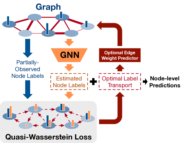
Figure 1: The scheme of our QW-loss and the corresponding learning paradigm. Given a graph whose node features are denoted as blue circles and partially-observed node labels are denoted as blue stems, a GNN embeds the graph nodes and outputs estimated labels (denoted as orange stems). By minimizing the QW loss, we obtain the optimal label transport (denoted as the dotted red arrows on the graph edges) between the real and estimated node labels. Optionally, the optimal label transport can be used to determine the weights of graph edges (through an edge weight predictor). The final predictions are the combinations of the optimal label transport and the estimated node labels.

To eliminate the inconsistency, we leverage computational optimal transport techniques Peyré and Cuturi 2019, proposing a new objective called Quasi-Wasserstein (QW) loss for learning GNNs. As illustrated in Figure 1, given partially-observed node labels and their estimations parametrized by a GNN, we consider the optimal transport between them and formulate the problem as the aggregation of the Wasserstein distances Frogner et al. 2015 corresponding to all label dimensions. This problem can be equivalently formulated as a label transport minimization problem Essid and Solomon 2018, Facca and Benzi 2021 defined on the graph, leading to the proposed QW loss. By minimizing this loss, we can jointly learn the optimal label transport and the GNN parametrizing the label estimations. This optimization problem can be solved efficiently by Bregman divergence-based algorithms, e.g., Bregman ADMM Wang and Banerjee 2014, Xu 2020. Optionally, through a multi-layer perceptron (MLP), we can determine the edge weights of the graph based on optimal label transport, leading to a GNN with learnable edge weights.

The contributions of this study include the following two points:

• A theoretically-solid loss without the inconsistency issue. The QW loss provides a new optimal transport-based loss for learning GNNs, which considers the labels and estimations of graph nodes jointly. Without the questionable i.i.d. assumption, it eliminates the inconsistency issue mentioned above. In theory, we demonstrate that the QW loss is a valid metric for the node labels defined on graphs. Additionally, the traditional objective function for learning GNNs can be treated as a special case of our QW loss. We further demonstrate that applying our QW loss reduces data fitting errors in the training phase.

• New learning and prediction paradigms. Different from the existing methods that combine GNNs with label propagation mechanisms Huang et al. 2021, Wang and Leskovec 2021, Dong et al. 2021, the QW loss provides a new way to combine node embeddings with label information in both training and testing phases. In particular, Bregman divergence-based algorithms are applied to learn the model, and the final model consists of the GNN and a residual component provided by the optimal label transport. When predicting node labels, the model combines the estimations provided by the GNN with the complementary information from the optimal label transport, leading to a new transductive prediction paradigm.

Experiments demonstrate that our QW loss applies to various GNNs and helps to improve their performance in various node-level classification and regression tasks.

2 Related work

2.1 Graph Neural Networks

Graph neural networks can be coarsely categorized into two classes. The GNNs in the first class apply spatial convolutions to graphs Niepert et al. 2016. The representative work includes the graph convolutional network (GCN) in Kipf and Welling 2017, the graph attention network (GAT) in Veličković et al. 2018, and their variants Zhuang and Ma 2018, Wang et al. 2019, Fu et al. 2020. The GNNs in the second class achieve graph spectral filtering Guo et al. 2023. They are often designed based on a polynomial basis, such as ChebNet Defferrard et al. 2016 and its variants He et al. 2022, GPR-GNN Chien et al. 2021, and BernNet He et al. 2021. Besides approximated by the polynomial basis, the spectral GNNs can be learned by other strategies, e.g., Personalized PageRank in APPNP Gasteiger et al. 2019, graph optimization functions in GNN-LF/HF Zhu et al. 2021, ARMA filters Bianchi et al. 2021, and diffusion kernel-based filters Klicpera et al. 2019, Xu et al. 2019c, Du et al. 2022.

The above spatial and spectral GNNs are correlated because a spatial convolution always corresponds to a graph spectral filter Balcilar et al. 2021. For example, GCN Kipf and Welling 2017 can be explained as a low-pass filter achieved by a first-order Chebyshev polynomial. Given a graph with some labeled nodes, we often learn the above GNNs in a semi-supervised node-level learning framework Kipf and Welling 2017, Yang et al. 2016, in which the GNNs embed all the nodes and are trained under the supervision of the labeled nodes. However, as aforementioned, the objective functions used in the framework treat the graph nodes independently and thus mismatch with the non-i.i.d. nature of the data.

2.2 Computational Optimal Transport

As a powerful mathematical tool, optimal transport (OT) distance (or called Wasserstein distance under some specific settings) provides a valid metric for probability measures Villani 2008, which has been widely used for various machine learning problems, e.g., distribution comparison Frogner et al. 2015, Lee et al. 2019, point cloud registration Grave et al. 2019, graph partitioning Dong and Sawin 2020, Xu et al. 2019b, generative modeling Arjovsky et al. 2017, Tolstikhin et al. 2018, and so on. Typically, the OT distance corresponds to a constrained linear programming problem. To approximate the OT distance with low complexity, many algorithms have been proposed, e.g., Sinkhorn-scaling Cuturi 2013, Bregman ADMM Wang and Banerjee 2014, Conditional Gradient Titouan et al. 2019, and Inexact Proximal Point Xie et al. 2020. Recently, two iterative optimization methods have been proposed to solve the optimal transport problems defined on graphs Essid and Solomon 2018, Facca and Benzi 2021.

These efficient algorithms make the OT distance a feasible loss for machine learning problems, e.g., the Wasserstein loss in Frogner et al. 2015. Focusing on the learning of GNNs, the work in Chen et al. 2020 proposes a Wasserstein distance-based contrastive learning method. The Gromovized Wasserstein loss is applied to learn cross-graph node embeddings Xu et al. 2019b, graph factorization models Vincent-Cuaz et al. 2021, Xu 2020, and GNN-based graph autoencoders Xu et al. 2022. The above work is designed for graph-level learning tasks, e.g., graph matching, representation, classification, and clustering. Our QW loss, on the contrary, is designed for node-level prediction tasks, resulting in significantly different learning and prediction paradigms.

3 Proposed Method

3.1 Motivation and Principle

Denote a graph as $G(\mathcal{V},\mathcal{E})$, where $\mathcal{V}$ represents the set of nodes and $\mathcal{E}$ represents the set of edges, respectively. The graph $G$ is associated with an adjacency matrix $\bm{A}\in\mathbb{R}^{|\mathcal{V}|\times|\mathcal{V}|}$ and a edge weight vector $\bm{w}=[w_{e}]\in\mathbb{R}^{|\mathcal{E}|}$. The weights in $\bm{w}$ correspond to the non-zero elements in $\bm{A}$. For an unweighted graph, $\bm{A}$ is a binary matrix, and $\bm{w}$ is an all-one vector. Additionally, the nodes of the graph may have $D$-dimensional features, which are formulated as a matrix $\bm{X}\in\mathbb{R}^{|\mathcal{V}|\times D}$. Suppose that a subset of nodes, denoted as $\mathcal{V}_{L}\subset\mathcal{V}$, are annotated with $C$-dimensional labels, i.e., $\{\bm{y}_{v}\in\mathbb{R}^{C}\}_{v\in\mathcal{V}_{L}}$. We would like to learn a GNN to predict the labels of the remaining nodes, i.e., $\{\bm{y}_{v}\}_{v\in\mathcal{V}\setminus\mathcal{V}_{L}}$.

The motivation for applying GNNs is based on the non-i.i.d. property of the node features and labels. Suppose that we have two nodes connected by an edge, i.e., $(v,v^{\prime})\in\mathcal{E}$, where $(\bm{x}_{v},\bm{y}_{v})$ and $(\bm{x}_{v^{\prime}},\bm{y}_{v^{\prime}})$ are their node features and labels. For each node, its neighbors’ features or labels can provide valuable information to its prediction task, i.e., the conditional probability $p(\bm{y}_{v}|\bm{x}_{v})\neq p(\bm{y}_{v}|\bm{x}_{v},\bm{x}_{v^{\prime}})$ and $p(\bm{y}_{v}|\bm{x}_{v})\neq p(\bm{y}_{v}|\bm{x}_{v},\bm{y}_{v^{\prime}})$ in general. Similarly, for node pairs, their labels are often conditionally-dependent, i.e., $p(\bm{y}_{v},\bm{y}_{v^{\prime}}|\bm{x}_{v},\bm{x}_{v^{\prime}})=p(\bm{y}_{v}|\bm{x}_{v},\bm{x}_{v^{\prime}},\bm{y}_{v^{\prime}})p(\bm{y}_{v^{\prime}}|\bm{x}_{v},\bm{x}_{v^{\prime}})\neq p(\bm{y}_{v}|\bm{x}_{v},\bm{x}_{v^{\prime}})p(\bm{y}_{v^{\prime}}|\bm{x}_{v},\bm{x}_{v^{\prime}})$. More generally, for all node labels, we have

$$\begin{aligned} p(\{\bm{y}_{v}\}_{v\in\mathcal{V}}|\bm{X},\bm{A})\neq\sideset{}{{}_{v\in\mathcal{V}}}{\prod}p(\bm{y}_{v}|\bm{X},\bm{A}),\end{aligned}$$ (1)

Ideally, we shall learn a GNN to maximize the conditional probability of all labeled nodes, i.e., $\max p(\{\bm{y}_{v}\}_{v\in\mathcal{V}_{L}}|\bm{X},\bm{A})$. In practice, however, most existing methods formulate the node-level learning paradigm of the GNN as

$$\sideset{}{{}_{\theta}}{\max}\sideset{}{{}_{v\in\mathcal{V}_{L}}}{\prod}p(\bm{y}_{v}|\bm{X},\bm{A};\theta)\Leftrightarrow\sideset{}{{}_{\theta}}{\min}\sideset{}{{}_{v\in\mathcal{V}_{L}}}{\sum}\psi(g_{v}(\bm{X},\bm{A};\theta),~{}\bm{y}_{v}).$$ (2)

Here, $g$ is a graph neural network whose parameters are denoted as $\theta$. Taking the adjacency matrix $\bm{A}$ and the node feature matrix $\bm{X}$ as input, the GNN $g$ predicts the node labels. $g_{v}(\bm{X},\bm{A};\theta)$ represents the estimation of the node $v$’s label achieved by the GNN, which is also denoted as $\hat{\bm{y}}_{v}$. Similarly, we denote $g_{\mathcal{V}}(\bm{X},\bm{A};\theta)$ as the estimated labels for the node set $\mathcal{V}$ in the following content. The loss function $\psi:\mathbb{R}^{C}\times\mathbb{R}^{C}\mapsto\mathbb{R}$ is defined in the node level. In node-level classification tasks, it is often implemented as the cross-entropy loss or the KL-divergence (i.e., $p(\bm{y}_{v}|\bm{X},\bm{A};\theta)$ is modeled by the softmax function). In node-level regression tasks, it is often implemented as the least-square loss (i.e., $p(\bm{y}_{v}|\bm{X},\bm{A};\theta)$ is assumed to be the Gaussian distribution).

The loss in (2) assumes the node labels to be conditionally-independent with each other, which may be too strong in practice and inconsistent with the non-i.i.d. property of graph-structured data shown in (1). To eliminate such inconsistency, we should treat node labels as a set rather than independent individuals, developing a set-level loss to penalize the discrepancy between the observed labels and their estimations globally, i.e.,

$$\sideset{}{{}_{\theta}}{\min}\text{Loss}(g_{\mathcal{V}_{L}}(\bm{X},\bm{A};\theta),\{\bm{y}_{v}\}_{v\in\mathcal{V}_{L}}).$$ (3)

In the following content, we will design such a loss with theoretical supports, based on the optimal transport on graphs.

3.2 Optimal Transport on Graphs

Suppose that we have two measures on a graph $G(\mathcal{V},\mathcal{E})$, denoted as $\bm{\mu}\in[0,\infty)^{|\mathcal{V}|}$ and $\bm{\gamma}\in[0,\infty)^{|\mathcal{V}|}$, respectively. The element of each measure indicates the “mass” of a node. Assume the two measures to be balanced, i.e., $\langle\bm{\gamma}-\bm{\mu},\bm{1}_{|\mathcal{V}|}\rangle=0$, where $\langle\cdot,\cdot\rangle$ is the inner product operator. The optimal transport, or called the 1-Wasserstein distance Villani 2008, between them is defined as

$$W_{1}(\bm{\mu},\bm{\gamma}):=\sideset{}{{}_{\bm{T}\in\Pi(\bm{\mu},\bm{\gamma})}}{\min}\langle\bm{D},~{}\bm{T}\rangle=\sideset{}{{}_{\bm{T}\in\Pi(\bm{\mu},\bm{\gamma})}}{\min}\sideset{}{{}_{v,v^{\prime}\in\mathcal{V}\times\mathcal{V}}}{\sum}t_{vv^{\prime}}d_{vv^{\prime}},$$ (4)

where $\bm{D}=[d_{vv^{\prime}}]\in\mathbb{R}^{|\mathcal{V}|\times|\mathcal{V}|}$ represents the shortest path distance matrix, and $\Pi(\bm{\mu},\bm{\gamma})=\{\bm{T}\geq\bm{0}|\bm{T}\bm{1}_{|\mathcal{V}|}=\bm{\mu},\bm{T}^{\top}\bm{1}_{|\mathcal{V}|}=\bm{\gamma}\}$ represents the set of all valid doubly stochastic matrices. Each $\bm{T}=[t_{vv^{\prime}}]\in\Pi(\bm{\mu},\bm{\gamma})$ is a transport plan matrix. The optimization problem in (4) corresponds to finding the optimal transport plan $\bm{T}^{*}=[t_{vv^{\prime}}^{*}]$ to minimize the “cost” of changing $\bm{\mu}$ to $\bm{\gamma}$, in which the cost is measured as the sum of “mass” $t_{vv^{\prime}}$ moved from node $v$ to node $v^{\prime}$ times distance $d_{vv^{\prime}}$.

3.2.1 Wasserstein Distance for Vectors on A Graph

For the optimal transport problem defined on graphs, we can simplify the problem in (4) by leveraging the underlying graph structures. As shown in Essid and Solomon 2018, Santambrogio 2015, given a graph $G(\mathcal{V},\mathcal{E})$, we can define a sparse matrix $\bm{S}_{\mathcal{V}}=[s_{ve}]\in\{0,\pm 1\}^{|\mathcal{V}|\times|\mathcal{E}|}$ to indicating the graph topology. For node $v$ and edge $e$, the corresponding element in $\bm{S}_{\mathcal{V}}$ is

$$\begin{aligned} s_{ve}=\begin{cases}1&\text{if $v$ is ``head'' of edge $e$}\\ -1&\text{if $v$ is ``tail'' of edge $e$}\\ 0&\text{otherwise.}\end{cases}\end{aligned}$$ (5)

When $G$ is directed, the “head” and “tail” of each edge are predefined. When $G$ is undirected, we can randomly define each edge’s “head” and “tail”. Accordingly, the 1-Wasserstein distance in (4) can be equivalently formulated as a minimum-cost flow problem:

$$\begin{aligned} W_{1}(\bm{\mu},\bm{\gamma})=\sideset{}{{}_{\bm{f}\in\Omega(\bm{S}_{\mathcal{V}},\bm{\mu},\bm{\gamma})}}{\min}\|\text{diag}(\bm{w})\bm{f}\|_{1},\end{aligned}$$ (6)

where $\text{diag}(\bm{w})$ is a diagonal matrix constructed by the edge weights of the graph. The vector $\bm{f}=[f_{e}]\in\Omega(\bm{S}_{\mathcal{V}},\bm{\mu},\bm{\gamma})$ is the flow indicating the mass passing through each edge. Accordingly, the cost corresponding to edge $e$ is represented as the distance $w_{e}$ times the mass $f_{e}$, and the sum of all the costs leads to the objective function in (6). The feasible domain of the flow vector is defined as

$$\begin{aligned} \Omega(\bm{S}_{\mathcal{V}},\bm{\mu},\bm{\gamma})=\mathcal{U}^{|\mathcal{E}|}\cap\{\bm{f}~{}|~{}\bm{S}_{\mathcal{V}}\bm{f}=\bm{\gamma}-\bm{\mu}\},\quad\text{where}~{}\mathcal{U}=\begin{cases}[0,\infty),&\text{Directed $G$},\\ \mathbb{R},&\text{Undirected $G$}.\end{cases}\end{aligned}$$ (7)

The constraint $\bm{S}_{\mathcal{V}}\bm{f}=\bm{\gamma}-\bm{\mu}$ ensures that the flow on all the edges leads to the change from $\bm{\mu}$ to $\bm{\gamma}$. The flow in the directed graph is nonnegative, which can only pass through each edge from “head” to “tail”. On the contrary, the undirected graph allows the mass to transport from “tail” to “head”. By solving (6), we find the optimal flow $\bm{f}^{*}$ (or the so-called optimal transport on edges) that minimizes the overall cost $\|\text{diag}(\bm{w})\bm{f}\|_{1}$.

3.2.2 Partial Wasserstein Distance for Vectors on a Graph

When only a subset of nodes (i.e., $\mathcal{V}_{L}\subset\mathcal{V}$) have observable signals, we can define a partial Wasserstein distance on the graph by preserving the constraints relevant to $\mathcal{V}_{L}$: for $\bm{\mu},\bm{\gamma}\in\mathbb{R}^{|\mathcal{V}_{L}|}$, we have

$$\begin{aligned} W_{1}^{(P)}(\bm{\mu},\bm{\gamma})=\sideset{}{{}_{\bm{f}\in\Omega(\bm{S}_{\mathcal{V}_{L}},\bm{\mu},\bm{\gamma})}}{\min}\|\text{diag}(\bm{w})\bm{f}\|_{1},\end{aligned}$$ (8)

where $\bm{S}_{\mathcal{V}_{L}}\in\{0,\pm 1\}^{|\mathcal{V}_{L}|\times|\mathcal{E}|}$ is a submatrix of $\bm{S}_{\mathcal{V}}$, storing the rows corresponding to the nodes with observable signals.

Different from the classic Wasserstein distance, the Wasserstein distance defined on graphs is not limited for nonnegative vectors because the minimum-cost flow formulation in (6) is shift-invariant, i.e., $\forall\bm{\delta}\in\mathbb{R}^{|\mathcal{V}|}$, $W_{1}(\bm{\mu},\bm{\gamma})=W_{1}(\bm{\mu}-\bm{\delta},\bm{\gamma}-\bm{\delta})$. The partial Wasserstein distance in (8) can be viewed as a generalization of (6), and thus it holds the shift-invariance as well. Moreover, given an undirected graph, we can prove that both the $W_{1}$ in (6) and the $W_{1}^{(P)}$ in (8) can be valid metrics in the spaces determined by the topology of an undirected graph (See Appendix A for a complete proof).

Theorem 1 (The Validness as A Metric).

Given an undirected graph $G(\mathcal{V},\mathcal{E})$, with edge weights $\bm{w}\in[0,\infty)^{|\mathcal{E}|}$ and a matrix $\bm{S}_{\mathcal{V}}\in\{0,\pm 1\}^{|\mathcal{V}|\times\mathcal{E}}$ defined in (5), the $W_{1}$ in (6) is a metric in $Range(\bm{S}_{\mathcal{V}})$, and the $W_{1}^{(P)}$ in (8) is a metric in $Range(\bm{S}_{\mathcal{V}_{L}})$, $\forall\mathcal{V}_{L}\in\mathcal{V}$.

The flow vector $\bm{f}$ in (8) has fewer constraints than that in (6), so the relation between $W_{1}$ and $W_{1}^{(P)}$ obeys the following theorem.

Theorem 2 (The Monotonicity).

Given an undirected graph $G(\mathcal{V},\mathcal{E})$, with edge weights $\bm{w}\in[0,\infty)^{|\mathcal{E}|}$ and a matrix $\bm{S}_{\mathcal{V}}\in\{0,\pm 1\}^{|\mathcal{V}|\times\mathcal{E}}$ defined in (5), we have

$$\begin{aligned} W_{1}(\bm{\mu},\bm{\gamma})\geq W_{1}^{(P)}(\bm{\mu}_{\mathcal{V}^{\prime}},\bm{\gamma}_{\mathcal{V}^{\prime}})\geq W_{1}^{(P)}(\bm{\mu}_{\mathcal{V}^{\prime\prime}},\bm{\gamma}_{\mathcal{V}^{\prime\prime}})\geq 0,\quad\forall\bm{\mu},\bm{\gamma}\in Range(\bm{S}_{\mathcal{V}}),~{}\mathcal{V}^{\prime\prime}\subset\mathcal{V}^{\prime}\subset\mathcal{V},\end{aligned}$$ (9)

where $\bm{\mu}_{\mathcal{V}^{\prime}}$ denotes the subvector of $\bm{\mu}$ corresponding to the set $\mathcal{V}^{\prime}$.

3.3 Learning GNNs with Quasi-Wasserstein Loss

Inspired by the optimal transport on graphs, we propose a Quasi-Wasserstein loss for learning GNNs. Given a partially-labeled graph $G$, we formulate observed labels as a matrix $\bm{Y}_{\mathcal{V}_{L}}=[\bm{y}_{\mathcal{V}_{L}}^{(c)}]\in\mathbb{R}^{|\mathcal{V}_{L}|\times C}$, where $\bm{y}_{\mathcal{V}_{L}}^{(c)}\in\mathbb{R}^{|\mathcal{V}_{L}|}$ represents the labels in $c$-th dimension. The estimated labels generated by a GNN $g$ are represented as $\widehat{\bm{Y}}_{\mathcal{V}_{L}}=[\hat{\bm{y}}_{\mathcal{V}_{L}}^{(c)}]:=g_{\mathcal{V}_{L}}(\bm{X},\bm{A};\theta)$. Our QW loss is defined as

$$\begin{aligned} QW(\widehat{\bm{Y}}_{\mathcal{V}_{L}},\bm{Y}_{\mathcal{V}_{L}})&=\sideset{}{{}_{c=1}^{C}}{\sum}W_{1}^{(P)}(\hat{\bm{y}}_{\mathcal{V}_{L}}^{(c)},\bm{y}_{\mathcal{V}_{L}}^{(c)})\\ &=\sideset{}{{}_{c=1}^{C}}{\sum}\sideset{}{{}_{\bm{f}^{(c)}\in\Omega(\bm{S}_{\mathcal{V}_{L}},~{}\hat{\bm{y}}_{\mathcal{V}_{L}}^{(c)},~{}\bm{y}_{\mathcal{V}_{L}}^{(c)})}}{\min}\|\text{diag}(\bm{w})\bm{f}^{(c)}\|_{1}\\ &=\sideset{}{{}_{\bm{F}\in\Omega_{C}(\bm{S}_{\mathcal{V}_{L}},~{}g_{\mathcal{V}_{L}}(\bm{X},\bm{A};\theta),~{}\bm{Y}_{\mathcal{V}_{L}})}}{\min}\|\text{diag}(\bm{w})\bm{F}\|_{1},\end{aligned}$$ (10)

where $\bm{F}=[\bm{f}^{(c)}]$ is the flow matrix, and its feasible domain $\Omega_{C}=\mathcal{U}^{|\mathcal{E}|\times C}\cap\{\bm{F}|\bm{S}_{\mathcal{V}_{L}}\bm{F}=\bm{Y}_{\mathcal{V}_{L}}-g_{\mathcal{V}_{L}}(\bm{X},\bm{A};\theta)\}$. $W_{1}^{(P)}(\hat{\bm{y}}_{\mathcal{V}_{L}}^{(c)},\bm{y}_{\mathcal{V}_{L}}^{(c)})$ is the partial Wasserstein distance between the observed and estimated labels in the $c$-th dimension. The QW loss is the summation of the $C$ partial Wasserstein distances, and it can be rewritten as the summation of $C$ minimum-cost flow problems. As shown in the third row of (10), these $C$ problems can be formulated as a single optimization problem, and the variables of the problems are aggregated as the flow matrix $\bm{F}$. Based on Theorem 1, our QW loss is a metric for the matrices whose columns are in $Range(\bm{S}_{\mathcal{V}_{L}})$.

The optimal flow matrix $\bm{F}^{*}=[\bm{f}^{(c)*}]$ is called optimal label transport in this study, in which the column $\bm{f}^{(c)*}$ indicating the optimal transport on graph edges between the observed labels and their estimations in the $c$-th dimension. Note that, we call the proposed loss “Quasi-Wasserstein” because $i)$ it is not equal to the classic 1-Wasserstein distance between the label sets $\widehat{\bm{Y}}_{\mathcal{V}_{L}}$ and $\bm{Y}_{\mathcal{V}_{L}}$ Peyré and Cuturi 2019, and $ii)$ the optimal label transport $\bm{F}^{*}$ cannot be reformulated as the optimal transport $\bm{T}^{*}$ obtained by (4). When $\bm{F}^{*}=\bm{0}$, we have $QW(\widehat{\bm{Y}}_{\mathcal{V}_{L}},\bm{Y}_{\mathcal{V}_{L}})=0$ and accordingly, $\widehat{\bm{Y}}_{\mathcal{V}_{L}}=\bm{Y}_{\mathcal{V}_{L}}$, which means that the GNN $g$ perfectly estimates the observed labels. Therefore, the QW loss provides a new alternative for the training loss of GNN. Different from the traditional loss function in (2), the QW loss treats observed node labels and their estimations as two sets and measures their discrepancy accordingly, which provides an effective implementation of the loss in (3).

Applying the QW loss to learn a GNN $g$ results in the following constrained optimization problem:

$$\begin{aligned} \sideset{}{{}_{\theta}}{\min}QW(g_{\mathcal{V}_{L}}(\bm{X},\bm{A};\theta),\bm{Y}_{\mathcal{V}_{L}})=\sideset{}{{}_{\theta}}{\min}\sideset{}{{}_{\bm{F}\in\Omega_{C}(\bm{S}_{\mathcal{V}_{L}},~{}g_{\mathcal{V}_{L}}(\bm{X},\bm{A};\theta),~{}\bm{Y}_{\mathcal{V}_{L}})}}{\min}\|\text{diag}(\bm{w})\bm{F}\|_{1}.\end{aligned}$$ (11)

To solve it effectively, we consider the following two algorithms.

3.3.1 Bregman Divergence-based Approximate Solver

By relaxing the constraint $\{\bm{F}|\bm{S}_{\mathcal{V}_{L}}\bm{F}=\bm{Y}_{\mathcal{V}_{L}}-g_{\mathcal{V}_{L}}(\bm{X},\bm{A};\theta)\}$ to a Bregman divergence-based regularizer Benamou et al. 2015, we can reformulate (11) to the following problem:

$$\begin{aligned} \sideset{}{{}_{\theta,~{}\bm{F}\in\mathcal{U}^{|\mathcal{E}|\times C}}}{\min}\|\text{diag}(\bm{w})\bm{F}\|_{1}+\lambda\underbrace{B_{\phi}(g_{\mathcal{V}_{L}}(\bm{X},\bm{A};\theta)+\bm{S}_{\mathcal{V}_{L}}\bm{F},~{}\bm{Y}_{\mathcal{V}_{L}})}_{\sum_{v\in\mathcal{V}_{L}}\psi(g_{v}(\bm{X},\bm{A};\theta)+\bm{S}_{v}\bm{F},~{}\bm{y}_{v})}.\end{aligned}$$ (12)

Here, $B_{\phi}(x,y)=\phi(x)-\phi(y)-\langle\nabla\phi(y),x-y\rangle$ is the Bregman divergence defined based on the strictly convex function $\phi$, and the hyperparameter $\lambda>0$ controls its significance. In node classification tasks, we can set $\phi$ as an entropic function, and the Bregman divergence becomes the KL-divergence. In node regression tasks, we can set $\phi$ as a least-square loss, and the Bregman divergence becomes the least-square loss. Therefore, as shown in (12), the Bregman divergence $B_{\phi}$ can be implemented based on commonly-used loss functions, e.g., the $\psi$ in (2).

Algorithm 1 Learning a GNN by solving (12)

0:  A graph $G$, its adjacency matrix $\bm{A}$ (edge weights $\bm{w}$), node features $\bm{X}$, and observed labels $\bm{Y}_{\mathcal{V}_{L}}$.

1:  Initialize $\theta^{(0)}$ and $\bm{F}^{(0)}$ randomly.

2:  while Not converge do

3:     Compute $\text{Loss}=\|\text{diag}(w)\bm{F}\|_{1}+\lambda B_{\phi}(g_{\mathcal{V}_{L}}(\bm{X},\bm{A};\theta)+\bm{S}_{\mathcal{V}_{L}}\bm{F},\bm{Y}_{\mathcal{V}_{L}})$

4:     Update $\{\bm{F},\theta\}$ by Adam Kingma and Ba 2014.

5:     if $G$ is a directed graph then $\bm{F}\leftarrow\text{Proj}_{\geq 0}(\bm{F})$ end if.

6:  end while

7:  return  Optimal label transport $\bm{F}^{*}$ and model parameters $\theta^{*}$.

Algorithm 1 shows the algorithmic scheme in details. For undirected graphs, the $\mathcal{U}$ in (12) is $\mathbb{R}$, and accordingly, (12) becomes a unconstrained optimization problem. We can solve it efficiently by gradient descent. For directed graphs, we just need to add a projection step when updating the flow matrix $\bm{F}$, leading to the projected gradient descent algorithm.

3.3.2 Bregman ADMM-based Exact Solver

Algorithm 1 solves  (11) approximately — because of relaxing the strict equality constraint to a regularizer, the solution of (12) often cannot satisfy the original equality constraint. To solve (11) exactly, we further develop a learning method based on the Bregman ADMM (Bremgan Alternating Direction Method of Multipliers) algorithm Wang and Banerjee 2014. In particular, we can rewrite (11) in the following augmented Lagrangian form:

$$\begin{aligned} \sideset{}{{}_{\theta,~{}\bm{F}\in\mathcal{U}^{|\mathcal{E}|\times C},~{}\bm{Z}\in\mathbb{R}^{|\mathcal{V}_{L}|\times C}}}{\min}&\|\text{diag}(\bm{w})\bm{F}\|_{1}+\langle\bm{Z},~{}g_{\mathcal{V}_{L}}(\bm{X},\bm{A};\theta)+\bm{S}_{\mathcal{V}_{L}}\bm{F}-\bm{Y}_{\mathcal{V}_{L}}\rangle\\ &+\lambda B_{\phi}(g_{\mathcal{V}_{L}}(\bm{X},\bm{A};\theta)+\bm{S}_{\mathcal{V}_{L}}\bm{F},~{}\bm{Y}_{\mathcal{V}_{L}}),\end{aligned}$$ (13)

where $\bm{Z}\in\mathbb{R}^{|\mathcal{V}_{L}|\times C}$ is the dual variable, the second term in (13) is the Lagrangian term corresponding to the equality constraint, and the third term in (13) is the augmented term implemented as the Bregman divergence.

Algorithm 2 Learning a GNN by solving (13)

0:  A graph $G$, its adjacency matrix $\bm{A}$ (edge weights $\bm{w}$), node features $\bm{X}$, observed labels $\bm{Y}_{\mathcal{V}_{L}}$, the number of inner iterations $J$.

1:  Initialize $\theta^{(0)}$ and $\bm{F}^{(0)}$ randomly and set $\bm{Z}^{(0)}=\bm{0}_{|\mathcal{V}_{L}|\times C}$.

2:  while Not converge do

3:     Solve (14) by Adam Kingma and Ba 2014 with $J$ steps and obtain $\theta^{(k+1)}$.

4:     Solve (15) by Adam Kingma and Ba 2014 with $J$ steps and obtain $\bm{F}^{(k+1)}$.

5:     if $G$ is a directed graph then $\bm{F}^{(k+1)}\leftarrow\text{Proj}_{\geq 0}(\bm{F}^{(k+1)})$ end if.

6:     Obtain $\bm{Z}^{(k+1)}$ by (16).

7:  end while

8:  return  Optimal label transport $\bm{F}^{*}$ and model parameters $\theta^{*}$.

Denote the objective function in (13) as $L(\theta,\bm{F},\bm{Z})$. In the Bregman ADMM framework, we can optimize $\theta$, $\bm{F}$, and $\bm{Z}$ iteratively through alternating optimization. In the $k$-th iteration, we update the three variables via solving the following three subproblems:

$$\begin{aligned} \theta^{(k+1)}=&\arg\sideset{}{{}_{\theta}}{\min}L(\theta,\bm{F}^{(k)},\bm{Z}^{(k)})\\ =&\arg\sideset{}{{}_{\theta}}{\min}\langle\bm{Z}^{(k)},~{}g_{\mathcal{V}_{L}}(\bm{X},\bm{A};\theta)\rangle+\lambda B_{\phi}(g_{\mathcal{V}_{L}}(\bm{X},\bm{A};\theta)+\bm{S}_{\mathcal{V}_{L}}\bm{F}^{(k)},~{}\bm{Y}_{\mathcal{V}_{L}}).\end{aligned}$$ (14)

$$\begin{aligned} \bm{F}^{(k+1)}=&\arg\sideset{}{{}_{\bm{F}\in\mathcal{U}^{|\mathcal{E}|\times C}}}{\min}L(\theta^{(k+1)},\bm{F},\bm{Z}^{(k)})\\ =&\arg\sideset{}{{}_{\bm{F}\in\mathcal{U}^{|\mathcal{E}|\times C}}}{\min}\langle\bm{Z}^{(k)},~{}\bm{S}_{\mathcal{V}_{L}}\bm{F}\rangle+\lambda B_{\phi}(g_{\mathcal{V}_{L}}(\bm{X},\bm{A};\theta^{(k+1)})+\bm{S}_{\mathcal{V}_{L}}\bm{F},~{}\bm{Y}_{\mathcal{V}_{L}}).\end{aligned}$$ (15)

$$\bm{Z}^{(k+1)}=\bm{Z}^{(k)}+\lambda(g_{\mathcal{V}_{L}}(\bm{X},\bm{A};\theta^{(k+1)})+\bm{S}_{\mathcal{V}_{L}}\bm{F}^{(k+1)}-\bm{Y}_{\mathcal{V}_{L}}).$$ (16)

We can find that (14) is a unconstrained optimization problem, so we can update the model parameter $\theta$ by gradient descent. Similarly, we can solve (15) and update the flow matrix $\bm{F}$ by gradient descent or projected gradient descent, depending on whether the graph is undirected or not. Finally, the update of the dual variable $\bm{Z}$ can be achieved in a closed form, as shown in (16). The Bregman ADMM algorithm solves the original problem in (12) rather than a relaxed version. In theory, with the increase of iterations, we can obtain the optimal variables that satisfy the equality constraint. Algorithm 2 shows the scheme of the Bregman ADMM-based solver.

3.3.3 Optional Edge Weight Prediction

Some GNNs, e.g., GCN-LPA Wang and Leskovec 2021 and GAT Veličković et al. 2018, model the adjacency matrix of graph as learnable parameters. Inspired by these models, we can optionally introduce an edge weight predictor and parameterize the adjacency matrix based on the flow matrix, as shown in Figure 1. In particular, given $\bm{F}$, we can apply a multi-layer perceptron (MLP) to embed it to an edge weight vector and then obtain a weighted adjacency matrix. Accordingly, the learning problem becomes

$$\sideset{}{{}_{\theta,\xi}}{\min}\sideset{}{{}_{\bm{F}\in\Omega_{C}(\bm{S}_{\mathcal{V}_{L}},g_{\mathcal{V}_{L}}(\bm{X},\bm{A}(\bm{F};\xi);\theta),\bm{Y}_{\mathcal{V}_{L}})}}{\min}\|\text{diag}(\bm{w})\bm{F}\|_{1},$$ (17)

where $\bm{A}(\bm{F};\xi)$ represents the adjacency matrix determined by the label transportation $\bm{F}$, and $\xi$ represents the parameters of the MLP. Taking the learning of $\xi$ into account, we can modify the above two solvers slightly and make them applicable for solving (17).

Table 1: Comparison between traditional methods and ours

Method	Setting	Node Classification	Node Regression
Apply the	$\psi$	Cross-entropy or KL	Least-square
loss in (2)	Predicted $\bm{y}_{v}$	$g_{v}(\bm{X},\bm{A};\theta)$, $\forall v\in\mathcal{V}\setminus\mathcal{V}_{L}$
Apply the	$\phi$	Entropy	$\frac{1}{2}\|\cdot\|_{2}^{2}$
QW loss	$B_{\phi}(=\psi)$	KL	Least-square
	Predicted $\bm{y}_{v}$	$g_{v}(\bm{X},\bm{A};\theta)+\bm{S}_{v}\bm{F}$, $\forall v\in\mathcal{V}\setminus\mathcal{V}_{L}$

3.4 Connections to Traditional Methods

As discussed in Section 3.3.1 and shown in (12), the Bregman divergence $B_{\phi}$ can be implemented as the commonly-used loss function $\psi$ in (2) (e.g., the KL divergence or the least-square loss). Table 1 compares the typical setting of traditional learning methods and that of our QW loss-based method in different node-level tasks. Essentially, the traditional learning method in (2) can be viewed as a special case of our QW loss-based learning method. In particular, when setting $\bm{F}=\bm{0}_{|\mathcal{E}|\times C}$ and $B_{\phi}=\psi$, the objective function in (12) degrades to the objective function in (2), which treats each node independently. Similarly, when further setting the dual variable $\bm{Z}=\bm{0}_{|\mathcal{V}_{L}|\times C}$, the objective function in (13) degrades to the objective function in (2) as well. In theory, we demonstrate that our QW loss-based learning method can fit training data better than the traditional method does, as shown in the following theorem.

Theorem 3.

Let $\{\theta^{\star},\bm{F}^{\star},\bm{Z}^{\star}\}$ be the global optimal solution of (13), $\{\theta^{{\dagger}},\bm{F}^{{\dagger}}\}$ be the global optimal solution of (12), and $\theta^{{\ddagger}}$ be the global optimal solution of $\min_{\theta}B_{\phi}(g_{\mathcal{V}_{L}}(\bm{X},\bm{A};\theta),~{}\bm{Y}_{\mathcal{V}_{L}})$, we have

$$\begin{aligned} B_{\phi}(g_{\mathcal{V}_{L}}(\bm{X},\bm{A};\theta^{\star})+\bm{S}_{\mathcal{V}_{L}}\bm{F}^{\star},~{}\bm{Y}_{\mathcal{V}_{L}})\leq B_{\phi}(g_{\mathcal{V}_{L}}(\bm{X},\bm{A};\theta^{{\dagger}})+\bm{S}_{\mathcal{V}_{L}}\bm{F}^{{\dagger}},~{}\bm{Y}_{\mathcal{V}_{L}})\leq B_{\phi}(g_{\mathcal{V}_{L}}(\bm{X},\bm{A};\theta^{{\ddagger}}),~{}\bm{Y}_{\mathcal{V}_{L}})\end{aligned}$$

Proof.

The proof is straightforward — $\{\theta^{{\ddagger}},\bm{0}_{|\mathcal{E}|\times C}\}$ is a feasible solution of (12), so the corresponding objective is equal to or larger than that obtained by $\{\theta^{{\dagger}},\bm{F}^{{\dagger}}\}$. Similarly, $\{\theta^{{\dagger}},\bm{F}^{{\dagger}},\bm{0}_{|\mathcal{V}_{L}|\times C}\}$ is a feasible solution of (13), so the corresponding objective is equal to or larger than that obtained by $\{\theta^{\star},\bm{F}^{\star},\bm{Z}^{\star}\}$. ∎

Remark. It should be noted that although the Bregman ADMM-based solver can fit training data better in theory, in the cases with distribution shifting or out-of-distribution issues, it has a higher risk of over-fitting. Therefore, in practice, we can select one of the above two solvers to optimize the GW loss, depending on their performance. In the following experimental section, we will further compare these two solvers in details.

3.5 A New Transductive Prediction Paradigm

As shown in Table 1, given the learned model $\theta^{*}$ and the optimal label transport $\bm{F}^{*}$, we predict node labels in a new transductive prediction paradigm. For $v\in\mathcal{V}\setminus\mathcal{V}_{L}$, we predict its label as

$$\tilde{\bm{y}}_{v}:=g_{v}(\bm{X},\bm{A};\theta^{*})+\bm{S}_{v}\bm{F}^{*},$$ (18)

which combines the estimated label from the learned GNN and the residual component from the optimal label transport.

It should be noted that some attempts have been made to incorporate label propagation algorithms (LPAs) Zhu and Goldberg 2022 into GNNs, e.g., the GCN-LPA in Wang and Leskovec 2021 and the FDiff-Scale in Huang et al. 2021. The PTA in Dong et al. 2021 demonstrates that learning a decoupled GNN is equivalent to implementing a label propagation algorithm. These methods leverage LPAs to regularize the learning of GNNs. However, in the prediction phase, they abandon the training labels and rely only on the GNNs to predict node labels, as shown in Table 1. Unlike these methods, our QW loss-based method achieves a new kind of label propagation with the help of computational optimal transport, saving the training label information in the optimal label transport and applying it explicitly in the prediction phase.

Table 2: Basic information of the graphs and the comparisons on node classification accuracy (%).

Model

Method

Homophilic graphs

Heterophilic graphs

Overall

Cora

Citeseer

Pubmed

Computers

Photo

Squirrel

Chameleon

Actor

Texas

Cornell

Improve

#Nodes ($|\mathcal{V}|$)

2,708

3,327

19,717

13,752

5,201

7,650

2,277

7,600

183

183

#Features ($D$)

1,433

3,703

500

767

754

2,089

2,325

932

1,703

1,703

#Edges ($|\mathcal{E}|$)

5,278

4,552

44,324

245,861

119,081

198,358

31,371

26,659

279

277

Intra-edge rate

81.0$\%$

73.6$\%$

80.2$\%$

77.7$\%$

82.7$\%$

22.2$\%$

23.0$\%$

21.8$\%$

6.1$\%$

12.3$\%$

#Classes ($C$)

7

6

5

10

8

5

5

5

5

5

GCN

(2)

87.44${}_{\pm\text{0.96}}$

79.98${}_{\pm\text{0.84}}$

86.93${}_{\pm\text{0.29}}$

88.42${}_{\pm\text{0.45}}$

93.24${}_{\pm\text{0.43}}$

46.55${}_{\pm\text{1.15}}$

63.57${}_{\pm\text{1.16}}$

34.00${}_{\pm\text{1.28}}$

77.21${}_{\pm\text{3.28}}$

61.91${}_{\pm\text{5.11}}$

—

(2)+LPA

86.34${}_{\pm\text{1.45}}$

78.51${}_{\pm\text{1.22}}$

84.72${}_{\pm\text{0.70}}$

82.48${}_{\pm\text{0.69}}$

88.10${}_{\pm\text{1.31}}$

44.81${}_{\pm\text{1.81}}$

60.90${}_{\pm\text{1.63}}$

32.43${}_{\pm\text{1.59}}$

78.69${}_{\pm\text{6.47}}$

68.72${}_{\pm\text{5.95}}$

-1.36

QW

87.88${}_{\pm\text{0.79}}$

81.36${}_{\pm\text{0.41}}$

87.89${}_{\pm\text{0.40}}$

89.20${}_{\pm\text{0.41}}$

93.81${}_{\pm\text{0.36}}$

52.62${}_{\pm\text{0.49}}$

68.10${}_{\pm\text{1.01}}$

38.09${}_{\pm\text{0.50}}$

84.10${}_{\pm\text{2.95}}$

84.26${}_{\pm\text{2.98}}$

+4.81

GAT

(2)

89.20${}_{\pm\text{0.79}}$

80.75${}_{\pm\text{0.78}}$

87.42${}_{\pm\text{0.33}}$

90.08${}_{\pm\text{0.36}}$

94.38${}_{\pm\text{0.25}}$

48.20${}_{\pm\text{1.67}}$

64.31${}_{\pm\text{2.01}}$

35.68${}_{\pm\text{0.60}}$

80.00${}_{\pm\text{3.11}}$

68.09${}_{\pm\text{2.13}}$

—

QW

89.11${}_{\pm\text{0.66}}$

80.19${}_{\pm\text{0.64}}$

88.38${}_{\pm\text{0.23}}$

90.41${}_{\pm\text{0.28}}$

94.65${}_{\pm\text{0.24}}$

55.03${}_{\pm\text{1.35}}$

67.35${}_{\pm\text{1.42}}$

33.86${}_{\pm\text{2.13}}$

80.33${}_{\pm\text{1.80}}$

70.21${}_{\pm\text{2.13}}$

+1.14

GIN

(2)

86.22${}_{\pm\text{0.95}}$

76.18${}_{\pm\text{0.78}}$

87.87${}_{\pm\text{0.23}}$

80.87${}_{\pm\text{1.43}}$

89.83${}_{\pm\text{0.72}}$

39.11${}_{\pm\text{2.23 }}$

64.29${}_{\pm\text{1.51}}$

32.37${}_{\pm\text{1.56}}$

72.79${}_{\pm\text{4.92}}$

62.55${}_{\pm\text{4.80}}$

—

QW

86.24${}_{\pm\text{0.90}}$

76.13${}_{\pm\text{1.09}}$

87.53${}_{\pm\text{0.34}}$

89.28${}_{\pm\text{0.45}}$

92.60${}_{\pm\text{0.44}}$

65.29${}_{\pm\text{0.68}}$

73.26${}_{\pm\text{1.12}}$

32.32${}_{\pm\text{1.93}}$

77.54${}_{\pm\text{2.60}}$

64.04${}_{\pm\text{3.62}}$

+5.22

GraphSAGE

(2)

88.24${}_{\pm\text{0.95}}$

79.81${}_{\pm\text{0.80}}$

88.14${}_{\pm\text{0.25}}$

89.71${}_{\pm\text{0.38}}$

95.08${}_{\pm\text{0.26}}$

43.79${}_{\pm\text{0.59}}$

63.26${}_{\pm\text{1.09}}$

38.99${}_{\pm\text{0.85}}$

90.00${}_{\pm\text{2.30}}$

84.26${}_{\pm\text{2.98}}$

—

QW

87.59${}_{\pm\text{0.77}}$

80.52${}_{\pm\text{0.68}}$

88.61${}_{\pm\text{0.32}}$

90.17${}_{\pm\text{0.24}}$

95.25${}_{\pm\text{0.25}}$

54.37${}_{\pm\text{0.89}}$

68.32${}_{\pm\text{0.68}}$

37.82${}_{\pm\text{0.45}}$

90.33${}_{\pm\text{1.97}}$

86.38${}_{\pm\text{2.13}}$

+1.18

APPNP

(2)

88.14${}_{\pm\text{0.73}}$

80.47${}_{\pm\text{0.74}}$

88.12${}_{\pm\text{0.31}}$

85.32${}_{\pm\text{0.37}}$

88.51${}_{\pm\text{0.31}}$

36.15${}_{\pm\text{0.75}}$

52.93${}_{\pm\text{1.71}}$

40.46${}_{\pm\text{0.64}}$

91.31${}_{\pm\text{1.97}}$

87.66${}_{\pm\text{2.13}}$

—

QW

88.74${}_{\pm\text{0.84}}$

80.94${}_{\pm\text{0.61}}$

89.48${}_{\pm\text{0.28}}$

86.95 ${}_{\pm\text{0.82}}$

94.43${}_{\pm\text{0.24}}$

38.73${}_{\pm\text{1.06}}$

53.76${}_{\pm\text{1.25}}$

40.78${}_{\pm\text{0.74}}$

91.48${}_{\pm\text{2.30}}$

87.87${}_{\pm\text{2.34}}$

+1.41

BernNet

(2)

88.28${}_{\pm\text{1.00}}$

79.81${}_{\pm\text{0.79}}$

88.87${}_{\pm\text{0.38}}$

87.61${}_{\pm\text{0.46}}$

93.68${}_{\pm\text{0.28}}$

51.15${}_{\pm\text{1.09}}$

67.96${}_{\pm\text{1.05}}$

40.72${}_{\pm\text{0.80}}$

93.28${}_{\pm\text{1.48}}$

90.21${}_{\pm\text{2.35}}$

—

QW

89.03${}_{\pm\text{0.76}}$

81.35${}_{\pm\text{0.71}}$

89.03${}_{\pm\text{0.38}}$

89.58${}_{\pm\text{0.47}}$

94.55${}_{\pm\text{0.39}}$

55.22${}_{\pm\text{0.64}}$

71.66${}_{\pm\text{1.18}}$

40.91${}_{\pm\text{0.71}}$

93.44${}_{\pm\text{1.80}}$

90.85${}_{\pm\text{2.34}}$

+1.41

ChebNetII

(2)

88.26${}_{\pm\text{0.89}}$

80.00${}_{\pm\text{0.74}}$

88.57${}_{\pm\text{0.36}}$

86.58${}_{\pm\text{0.71}}$

93.50${}_{\pm\text{0.34}}$

57.78${}_{\pm\text{0.84}}$

71.71${}_{\pm\text{1.40}}$

40.70${}_{\pm\text{0.77}}$

92.79${}_{\pm\text{1.48}}$

88.94${}_{\pm\text{2.78}}$

—

QW

88.54${}_{\pm\text{0.76}}$

79.47${}_{\pm\text{0.70}}$

89.47${}_{\pm\text{0.36}}$

90.43${}_{\pm\text{0.22}}$

94.84${}_{\pm\text{0.37}}$

60.55${}_{\pm\text{0.64}}$

74.05${}_{\pm\text{0.68}}$

41.37${}_{\pm\text{0.67}}$

93.93${}_{\pm\text{0.98}}$

87.23${}_{\pm\text{3.62}}$

+1.11

4 Experiments

To demonstrate the effectiveness of our QW loss-based learning method, we apply it to learn GNNs with various architectures and test the learned GNNs in different node-level prediction tasks. We compare our learning method with the traditional one in (2) on their model performance and computational efficiency. For our method, we conduct a series of analytic experiments to show its robustness to hyperparameter settings and label insufficiency. All the experiments are conducted on a machine with three NVIDIA A40 GPUs, and the code is implemented based on PyTorch.

4.1 Implementation Details

4.1.1 Datasets

The datasets we considered consist of five homophilic graphs (i.e., Cora, Citeseer, Pubmed Sen et al. 2008, Yang et al. 2016, Computers, and Photo McAuley et al. 2015) and five heterophilic graphs (i.e., Chameleon, Squirrel Rozemberczki et al. 2021, Actor, Texas, and Cornell Pei et al. 2020), respectively. Following the work in Wang and Leskovec 2021, we categorize the graphs according to the percentage of the edges connecting the nodes of the same class (i.e., the intra-edge rate). The basic information of these graphs is shown in Table 2. Additionally, a large arXiv-year graph Lim et al. 2021 is applied to demonstrate the efficiency of our method. The adjacency matrix of each graph is binary, so the edge weights $\bm{w}=\bm{1}_{|\mathcal{E}|}$.

4.1.2 GNN Architectures

In the following experiments, the models we considered include $i)$ the representative spatial GNNs, i.e., GCN Kipf and Welling 2017, GAT Veličković et al. 2018, GIN Xu et al. 2019a, GraphSAGE Hamilton et al. 2017, and GCN-LPA Wang and Leskovec 2021 that combines the GCN with the label propagation algorithm; and $ii)$ state-of-the-art spectral GNNs, i.e., APPNP Gasteiger et al. 2019, BernNet He et al. 2021, and ChebNetII He et al. 2022. For a fair comparison, we set the architectures of the GNNs based on the code provided by He et al. 2022 and configure the algorithmic hyperparameters by grid search. More details of the hyperparameter settings are in Appendix.

4.1.3 Learning Tasks and Evaluation Measurements

For each graph, their nodes belong to different classes. Therefore, we first learn different GNNs to solve the node-level classification tasks defined on the above graphs. By default, the split ratio of each graph’s nodes is $60\%$ for training, $20\%$ for validation, and $20\%$ for testing, respectively. The GNNs are learned by $i)$ the traditional learning method in (2) and $ii)$ minimizing the proposed QW loss in (11), respectively. When implementing the QW loss, we apply either Algorithm 1 or 2, depending on their performance. Additionally, to demonstrate the usefulness of our QW loss in node-level regression tasks, we treat the node labels as one-hot vectors and fit them by minimizing the mean squared error (MSE), in which the $\psi$ in (2) and the corresponding Bregman divergence $B_{\phi}$ are set to be the least-square loss. For each method, we perform $10$ runs with different seeds and record the learning results’ mean and standard deviation.

4.2 Numerical Comparison and Visualization

4.2.1 Node Classification and Regression

Table 2 shows the node classification results on the ten graphs, whose last column records the overall improvements caused by our QW loss compared to other learning methods. The experimental results demonstrate the usefulness of our QW loss-based learning method — for each model, applying our QW loss helps to improve learning results in most situations and leads to consistent overall improvements. In particular, for the state-of-the-art spectral GNNs like BernNet He et al. 2021 and ChebNetII He et al. 2022, learning with our QW loss can improve their overall performance on both homophilic and heterophilic graphs consistently, resulting in the best performance in this experiment. For the simple GCN model Kipf and Welling 2017, learning with our QW loss improves its performance significantly and reduces the gap between its classification accuracy and that of the state-of-the-art models Gasteiger et al. 2019, He et al. 2021, 2022, especially heterophilic graphs. Note that, when learning GCN, our QW loss works better than the traditional method regularized by the label propagation (i.e., GCN-LPA Wang and Leskovec 2021) because our learning method can leverage the training label information in both learning and prediction phases. GCN-LPA improves GCN when learning on heterophilic graphs, but surprisingly, leads to performance degradation on homophilic graphs. Additionally, we also fit the one-hot labels by minimizing the MSE. As shown in Table 3, minimizing the QW loss leads to lower MSE results, which demonstrates the usefulness of the QW loss in node-level regression tasks.

Table 3: Comparisons on node regression error (MSE).

Model	Method	Homophilic graphs		Heterophilic graphs
		Computers	Photo	Actor	Cornell
GIN	(2)	0.0605${}_{\pm\text{0.0018}}$	0.0459${}_{\pm\text{0.0044}}$	0.1570${}_{\pm\text{0.0014}}$	0.1609${}_{\pm\text{0.0359}}$
	QW	0.0244${}_{\pm\text{0.0028}}$	0.0203${}_{\pm\text{0.0012}}$	0.1564${}_{\pm\text{0.0012}}$	0.1524${}_{\pm\text{0.0043}}$
BernNet	(2)	0.0871${}_{\pm\text{0.0002}}$	0.0488${}_{\pm\text{0.0009}}$	0.1661${}_{\pm\text{0.0020}}$	0.0989${}_{\pm\text{0.0076}}$
	QW	0.0364${}_{\pm\text{0.0038}}$	0.0297${}_{\pm\text{0.0014}}$	0.1671${}_{\pm\text{0.0008}}$	0.0753${}_{\pm\text{0.0024}}$

4.2.2 Computational Efficiency and Scalability

In theory, the computational complexity of our QW loss is linear with the number of edges. When implementing the loss as (13) and solving ti by Algorithm 2, its complexity is also linear with the number of inner iterations $J$. Figure 2 shows the runtime comparisons for the QW loss-based learning methods and the traditional method on two datasets. We can find that minimizing the QW loss by Algorithm 1 or Algorithm 2 with $J=1$ merely increases the training time slightly compared to the traditional method. Empirically, setting $J\leq 5$ can leads to promising learning results, as shown in Tables 2 and 3. In other words, the computational cost of applying the QW loss is tolerable considering the significant performance improvements it achieved. Additionally, we apply our QW loss to large-scale graphs and test its scalability. As shown in Table 4, we implement the QW loss based on Algorithm 1 (i.e., solving (12)) and apply it to the node classification task in the large-scale arXiv-year graph. The result shows that our QW loss is applicable to the graphs with millions of edges on a single GPU and improves the model performance.

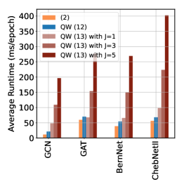
Figure 2: The runtime of different learning methods on the graph Photo.

Graph		arXiv-year
#Nodes ($|\mathcal{V}|$)		169,343
#Features ($D$)		128
#Edges ($|\mathcal{E}|$)		1,166,243
Intra-edge rate		22.0%
#Classes ($C$)		5
ChebNetII	(2)	48.18${}_{\pm\text{0.18}}$
	QW	48.30${}_{\pm\text{0.25}}$

Table 4: The node classification accuracy ($\%$) on a large graph.

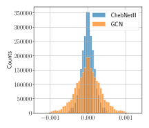
(a) Computers

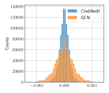
(b) Photo

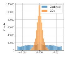
(c) Squirrel

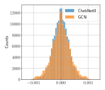
(d) Chameleon

Figure 3: The histogram of $\bm{F}$’s values for different GNNs.

4.2.3 Distribution of Optimal Label Transport

Figure 3 visualizes the histograms of the optimal label transport $\bm{F}^{*}$ learned for two representative GNNs (i.e., GCN Kipf and Welling 2017 and ChebNetII He et al. 2022) on four graphs (i.e., the homophilic graphs “Computers” and “Photo” and the heterophilic graphs “Squirrel” and “Chameleon”). We can find that when learning on homophilic graphs, the elements of the optimal label transport obey the zero-mean Laplacian distribution. It is reasonable from the perspective of optimization — the term $\|\text{diag}(\bm{w})\bm{F}\|_{1}$ can be explained as a Laplacian prior imposed on $\bm{F}$’s element. Additionally, we can find that the distribution corresponding to GCN has larger variance than that corresponding to ChebNetII, which implies that the $\bm{F}^{*}$ of GCN has more non-zero elements and thus has more significant impacts on label prediction. The numerical results in Table 2 can also verify this claim — in most situations, the performance improvements caused by the optimal label transport is significant for GCN but slight for ChebNetII. For heterophilic graphs, learning GCN still leads to Laplacian distributed label transport. However, the distributions corresponding to ChebNetII are diverse — the distribution for Squirrel is long-tailed while that for Chameleon is still Laplacian.

4.3 Analytic Experiments

4.3.1 Robustness to Label Insufficiency Issue

Our QW loss-based learning method considers the label transport on graphs, whose feasible domain is determined by the observed training labels. The more labels we observed, the smaller the feasible domain is. To demonstrate the robustness of our method to the label insufficiency issue, we evaluate the performance of our method given different amounts of training labels. We train ChebNetII He et al. 2022 on four graphs by traditional method and our method, respectively. For each graph, we use $K$% nodes’ labels to train the ChebNetII, where $K\in[1,60]$, and apply $20\%$ nodes for validation and $20\%$ nodes for testing, respectively, as the above default setting does. Figure 4 shows that our QW loss-based learning method can achieve encouraging performance even when only $20\%$ nodes or fewer are labeled. Additionally, the methods are robust to the selection of solver — we can minimize the QW loss based on (12) or (13), leading to comparable results and outperforming the traditional loss consistently.

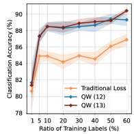
(a) Computers

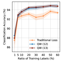
(b) Photo

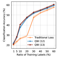
(c) Squirrel

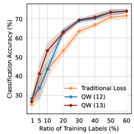
(d) Chameleon

Figure 4: Illustrations of the learning methods’ performance given different amounts of labeled nodes.

4.3.2 Impacts of Adjusting Edge Weights

As shown in (17), we can train an MLP to predict edge weights based on the optimal label transport. The ablation study in Table 5 quantitatively show the impacts of adjusting edge weights on the learning results. We can find that for ChebNetII, the two settings provide us with comparable learning results. For GCN, however, learning the model with adjusted edge weights suffers from performance degradation on homophilic graphs while leads to significant improvements on heterophilic graphs. Empirically, it seems that adjusting edge weights based on label transportation helps to improve the learning of simple GNN models on heterophilic graphs.

Table 5: Impacts of adjusting edge weights on node classification accuracy (%) when applying the QW loss.

Model		Homophilic		Heterophilic
		Computers	Photo	Actor	Cornell
GCN	$\bm{A}$	88.39${}_{\pm\text{0.55}}$	93.80${}_{\pm\text{0.37}}$	30.14${}_{\pm\text{0.80}}$	60.64${}_{\pm\text{4.26}}$
	$\bm{A}(\bm{F};\xi)$	84.35${}_{\pm\text{0.46}}$	91.79${}_{\pm\text{0.21}}$	38.09${}_{\pm\text{0.50}}$	84.26${}_{\pm\text{2.98}}$
ChebNetII	$\bm{A}$	89.52${}_{\pm\text{0.54}}$	94.84${}_{\pm\text{0.37}}$	41.37${}_{\pm\text{0.67}}$	86.38${}_{\pm\text{3.19}}$
	$\bm{A}(\bm{F};\xi)$	89.41${}_{\pm\text{0.41}}$	94.79${}_{\pm\text{0.45}}$	40.74${}_{\pm\text{0.80}}$	86.60${}_{\pm\text{2.98}}$

4.3.3 Robustness to Hyperparameters

The weight of the Bregman divergence term, i.e., $\lambda$, is the key hyperparameter impacting the performance of our learning method.

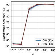
(a) Computers

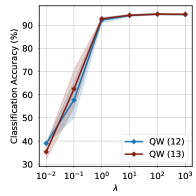
(b) Photo

(c) Squirrel

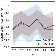
(d) Chameleon

Figure 5: Illustrations of the learning results achieved under different $\lambda$’s.

Empirically, when $\lambda$ is too small, the Bregman divergence between the observed labels and their predictions becomes ignorable. Accordingly, the regularizer may be too weak to supervise GNNs’ learning properly. On the contrary, when $\lambda$ is too large, the regularizer becomes dominant in the learning objective, and the impact of the label transport becomes weak in both the learning and prediction phases. As a result, it may perform similarly to the traditional method when using a large $\lambda$. We test the robustness of our method to $\lambda$ and show representative results in Figure 5. In particular, our QW loss-based method trains ChebNetII He et al. 2022 on four graphs. Both Algorithm 1 for (12) and Algorithm 2 for (13) are tested. The $\lambda$ is set in the range from $10^{-2}$ to $10^{3}$. For homophilic graphs, our learning method achieves stable performance when $\lambda\geq 10$. When $\lambda<10$, the learning results degrade significantly because of inadequate supervision. Our learning method often obtains the best learning result for heterophilic graphs when $\lambda\in[1,10]$. These experimental results show that our method is robust to the setting of $\lambda$, and we can set $\lambda$ in a wide range to obtain relatively stable performance.

5 Conclusion

We have proposed the Quasi-Wasserstein loss for learning graph neural networks. This loss matches well with the non-i.i.d. property of graph-structured data, providing a new strategy to leverage observed node labels in both training and testing phases. Applying the QW loss to learn GNNs improves their performance in various node-level prediction tasks. In the future, we would like to explore the impacts of the optimal label transport on the generalization power of GNNs in theory. Moreover, we plan to modify the QW loss further, developing a new optimization strategy to accelerate its computation.

Appendix A The Proofs of Theorems

A.1 Proof of Theorem 1

Proof.

The proof includes four parts:

• Feasibility. For $\bm{\mu},\bm{\gamma}\in\text{Range}(\bm{S}_{\mathcal{V}})$, we have

  $$W_{1}(\bm{\mu},\bm{\gamma})=\sideset{}{{}_{\bm{f}\in\Omega(\bm{S}_{\mathcal{V}},\bm{\mu},\bm{\gamma})}}{\min}\|\text{diag}(\bm{w})\bm{f}\|_{1}.$$ (19)

  Because $\bm{\mu},\bm{\gamma}\in\text{Range}(\bm{S}_{\mathcal{V}})$, the feasible domain $\Omega(\bm{S}_{\mathcal{V}},\bm{\mu},\bm{\gamma})$ is always non-empty and the optimization problem in (19) is always valid.

• Positivity. Obviously, the objective in (19) is nonnegative, so that $W_{1}(\bm{\mu},\bm{\gamma})\geq 0$, $\forall\bm{\mu},\bm{\gamma}\in\text{Range}(\bm{S}_{\mathcal{V}})$. Moreover, let

  $$\bm{f}^{*}=\arg\sideset{}{{}_{\bm{f}\in\Omega(\bm{S}_{\mathcal{V}},\bm{\mu},\bm{\gamma})}}{\min}\|\text{diag}(\bm{w})\bm{f}\|_{1}.$$

  $W_{1}(\bm{\mu},\bm{\gamma})=0$ when $\bm{f}^{*}=\bm{0}_{|\mathcal{E}|}$, which means $\bm{\mu}=\bm{\gamma}$. Therefore, $\forall\bm{\mu},\bm{\gamma}\in\text{Range}(\bm{S}_{\mathcal{V}})$, $W_{1}(\bm{\mu},\bm{\gamma})\geq 0$ and the equality holds iff $\bm{\mu}=\bm{\gamma}$.

• Symmetry. Obviously, if $\bm{f}^{*}$ is the optimal solution corresponding to $W_{1}(\bm{\mu},\bm{\gamma})$, $-\bm{f}^{*}$ will be the optimal solution of $W_{1}(\bm{\gamma},\bm{\mu})$. Because the edge weight vector is nonnegative, we have $\|\text{diag}(\bm{w})\bm{f}^{*}\|_{1}=\|-\text{diag}(\bm{w})\bm{f}^{*}\|_{1}$. As a result, $W_{1}(\bm{\mu},\bm{\gamma})=W_{1}(\bm{\gamma},\bm{\mu})$.

• Triangle Inequality. For $\bm{\mu},\bm{\gamma},\bm{\zeta}\in\text{Range}(\bm{S}_{\mathcal{V}})$, let

  $$\begin{aligned} &W_{1}(\bm{\mu},\bm{\gamma})=\sideset{}{{}_{\bm{f}_{1}\in\Omega(\bm{S}_{\mathcal{V}},\bm{\mu},\bm{\gamma})}}{\min}\|\text{diag}(\bm{w})\bm{f}_{1}\|_{1},\\ &W_{1}(\bm{\gamma},\bm{\zeta})=\sideset{}{{}_{\bm{f}_{2}\in\Omega(\bm{S}_{\mathcal{V}},\bm{\gamma},\bm{\zeta})}}{\min}\|\text{diag}(\bm{w})\bm{f}_{2}\|_{1}.\end{aligned}$$

  Then, we have

  $$\begin{aligned} W_{1}(\bm{\mu},\bm{\gamma})+W_{1}(\bm{\gamma},\bm{\zeta})=&\sideset{}{{}_{\bm{f}_{1}\in\in\Omega(\bm{S}_{\mathcal{V}},\bm{\mu},\bm{\gamma}),~{}\bm{f}_{2}\in\in\Omega(\bm{S}_{\mathcal{V}},\bm{\gamma},\bm{\zeta})}}{\min}\|\text{diag}(\bm{w})\bm{f}_{1}\|_{1}+\|\text{diag}(\bm{w})\bm{f}_{2}\|_{1}\\ \geq&\sideset{}{{}_{\bm{f}_{1},~{}\bm{f}_{2}\in\mathbb{R}^{|\mathcal{E}|},~{}\bm{S}_{\mathcal{V}}(\bm{f}_{1}+\bm{f}_{2})=\bm{\zeta}-\bm{\mu}}}{\min}\|\text{diag}(\bm{w})\bm{f}_{1}\|_{1}+\|\text{diag}(\bm{w})\bm{f}_{2}\|_{1}\\ =&\sideset{}{{}_{\bm{\tau},~{}\bm{\delta}\in\mathbb{R}^{|\mathcal{E}|},~{}2\bm{S}_{\mathcal{V}}\bm{\tau}=\bm{\zeta}-\bm{\mu}}}{\min}\|\text{diag}(\bm{w})\bm{\tau}+\bm{\delta}\|_{1}+\|\text{diag}(\bm{w})\bm{\tau}-\bm{\delta}\|_{1}\\ =&\|\text{diag}(\bm{w})\hat{\bm{\tau}}+\hat{\bm{\delta}}\|_{1}+\|\text{diag}(\bm{w})\hat{\bm{\tau}}-\hat{\bm{\delta}}\|_{1}\\ \geq&\|2\text{diag}(\bm{w})\hat{\bm{\tau}}\|_{1}\\ \geq&\sideset{}{{}_{\bm{f}\in\Omega(\bm{S}_{\mathcal{V}},\bm{\mu},\bm{\zeta})}}{\min}\|\text{diag}(\bm{w})\bm{f}\|_{1}\\ =&W_{1}(\bm{\mu},\bm{\zeta}).\end{aligned}$$ (20)

  Here, $\bm{\delta}:=0.5\text{diag}(\bm{w})(\bm{f}_{1}-\bm{f}_{2})$, $\bm{\tau}:=0.5(\bm{f}_{1}+\bm{f}_{2})$, and

  $$\begin{aligned} \hat{\bm{\tau}},\hat{\bm{\delta}}=&\arg\sideset{}{{}_{\bm{\tau},\bm{\delta}\in\mathbb{R}^{|\mathcal{E}|},~{}2\bm{S}_{\mathcal{V}}\bm{\tau}=\bm{\zeta}-\bm{\mu}}}{\min}\|\text{diag}(\bm{w})\bm{\tau}+\bm{\delta}\|_{1}+\|\text{diag}(\bm{w})\bm{\tau}-\bm{\delta}\|_{1}.\end{aligned}$$

  In (20), the first inequality is because the number of constraints is reduced and the feasible domain becomes larger. The second inequality leverages the triangular inequality of $\ell_{1}$-norm. The third inequality is because $2\hat{\bm{\tau}}$ is a feasible solution (rather than the optimal solution) corresponding to $W_{1}(\bm{\mu},\bm{\zeta})$.

Replacing $\mathcal{V}$ to a subset of nodes $\mathcal{V}^{\prime}\subset\mathcal{V}$, we obtain a partial Wasserstein distance $W_{1}^{(P)}$ defined on the graph. Based on the same steps, we can prove that $W_{1}^{(P)}$ is a valid metric in $\text{Range}(\bm{S}_{\mathcal{V}^{\prime}})$. ∎

A.2 The Proof of Theorem 2

Proof.

Denote $\mathcal{V}_{U}=\mathcal{V}\setminus\mathcal{V}^{\prime}$. Based on the shrinkage of the feasible domain, we have

$$\begin{aligned} W_{1}(\bm{\mu},\bm{\gamma})&=\sideset{}{{}_{\bm{f}\in\Omega(\bm{S}_{\mathcal{V}},\bm{\mu},\bm{\gamma})}}{\min}\|\text{diag}(\bm{w})\bm{f}\|_{1}\\ &=\sideset{}{{}_{\bm{f}\in\Omega(\bm{S}_{\mathcal{V}^{\prime}},\bm{\mu}_{\mathcal{V}^{\prime}},\bm{\gamma}_{\mathcal{V}^{\prime}})\cap\Omega(\bm{S}_{\mathcal{V}_{U}},\bm{\mu}_{\mathcal{V}_{U}},\bm{\gamma}_{\mathcal{V}U})}}{\min}\|\text{diag}(\bm{w})\bm{f}\|_{1}\\ &\geq\sideset{}{{}_{\bm{f}\in\Omega(\bm{S}_{\mathcal{V}^{\prime}},\bm{\mu}_{\mathcal{V}^{\prime}},\bm{\gamma}_{\mathcal{V}^{\prime}})}}{\min}\|\text{diag}(\bm{w})\bm{f}\|_{1}=W_{1}^{(P)}(\bm{\mu}_{\mathcal{V}^{\prime}},\bm{\gamma}_{\mathcal{V}^{\prime}}).\end{aligned}$$

The second inequality in (9) can be proven in the same way. The nonnegativeness is based on the metricity. ∎

Appendix B Experimental Details

B.1 Baseline Implementations and Experimental Settings

All baseline models are implemented using the code released by the respective authors, as provided below.

• GCN, GAT, APPNP, and BernNet: https://github.com/ivam-he/BernNet

• ChebNetII: https://github.com/ivam-he/ChebNetII

• GCN-LPA: https://github.com/hwwang55/GCN-LPA

For GCN, GAT, GIN, GraphSAGE, and APPNP, we search the learning rate over the range of $\{0.001,0.002,0.01,0.05\}$ and the weight decay over the range of $\{0.0,0.0005\}$. For APPNP, we search its key hyperparameter $\alpha$ over $\{0.1,0.2,0.5,0.9\}$. For BernNet and ChebNetII, we used the hyperparameters provided by the original papers He et al. 2021, 2022. For GCN-LPA, we apply a two-layer GCN associated with five LPA iteration layers, which follows the settings in Wang and Leskovec 2021. We utilize the same datasets and data partitioning as BernNet He et al. 2021 and ChebNetII He et al. 2022 in our experiments.

B.2 Hyperparameter Settings

For all GNN methods, we modify their architectures according to Algorithms 1 and 2 and learn the models through the QW loss. The key hyperparameters and their search spaces are shown below: $A_{F}$ indicates whether the optimal label transport is involved in the adjustment of edge weights, which is set to True or False. $\lambda$ is the weights of Bergman divergence, whose search space is $\{10^{-2},10^{-1},...,10^{3}\}$. $lr_{F}$ and $L_{F}$ denote the learning rate and weight decay for the label transport $\bm{F}$ and MLP-based edge weight predictor. We search for parameter $lr_{F}$ over the range of $\{0.001,0.002,0.01,0.05\}$ and parameter $L_{F}$ over the range of $\{0.0,0.0005\}$.

References

- 1
- Arjovsky et al. 2017 Martin Arjovsky, Soumith Chintala, and Léon Bottou. 2017. Wasserstein generative adversarial networks. In International conference on machine learning. PMLR, 214–223.
- Balcilar et al. 2021 Muhammet Balcilar, Renton Guillaume, Pierre Héroux, Benoit Gaüzère, Sébastien Adam, and Paul Honeine. 2021. Analyzing the expressive power of graph neural networks in a spectral perspective. In Proceedings of the International Conference on Learning Representations (ICLR).
- Benamou et al. 2015 Jean-David Benamou, Guillaume Carlier, Marco Cuturi, Luca Nenna, and Gabriel Peyré. 2015. Iterative Bregman projections for regularized transportation problems. SIAM Journal on Scientific Computing 37, 2 (2015), A1111–A1138.
- Bianchi et al. 2021 Filippo Maria Bianchi, Daniele Grattarola, Lorenzo Livi, and Cesare Alippi. 2021. Graph neural networks with convolutional arma filters. IEEE transactions on pattern analysis and machine intelligence 44, 7 (2021), 3496–3507.
- Chen et al. 2020 Benson Chen, Gary Bécigneul, Octavian-Eugen Ganea, Regina Barzilay, and Tommi Jaakkola. 2020. Optimal transport graph neural networks. arXiv preprint arXiv:2006.04804 (2020).
- Chien et al. 2021 Eli Chien, Jianhao Peng, Pan Li, and Olgica Milenkovic. 2021. Adaptive Universal Generalized PageRank Graph Neural Network. In International Conference on Learning Representations.
- Cuturi 2013 Marco Cuturi. 2013. Sinkhorn distances: lightspeed computation of optimal transport. In Proceedings of the 26th International Conference on Neural Information Processing Systems-Volume 2. 2292–2300.
- Defferrard et al. 2016 Michaël Defferrard, Xavier Bresson, and Pierre Vandergheynst. 2016. Convolutional neural networks on graphs with fast localized spectral filtering. Advances in neural information processing systems 29 (2016).
- Dong et al. 2021 Hande Dong, Jiawei Chen, Fuli Feng, Xiangnan He, Shuxian Bi, Zhaolin Ding, and Peng Cui. 2021. On the equivalence of decoupled graph convolution network and label propagation. In Proceedings of the Web Conference 2021. 3651–3662.
- Dong and Sawin 2020 Yihe Dong and Will Sawin. 2020. Copt: Coordinated optimal transport on graphs. Advances in Neural Information Processing Systems 33 (2020), 19327–19338.
- Du et al. 2022 Lun Du, Xiaozhou Shi, Qiang Fu, Xiaojun Ma, Hengyu Liu, Shi Han, and Dongmei Zhang. 2022. Gbk-gnn: Gated bi-kernel graph neural networks for modeling both homophily and heterophily. In Proceedings of the ACM Web Conference 2022. 1550–1558.
- Essid and Solomon 2018 Montacer Essid and Justin Solomon. 2018. Quadratically regularized optimal transport on graphs. SIAM Journal on Scientific Computing 40, 4 (2018), A1961–A1986.
- Facca and Benzi 2021 Enrico Facca and Michele Benzi. 2021. Fast iterative solution of the optimal transport problem on graphs. SIAM Journal on Scientific Computing 43, 3 (2021), A2295–A2319.
- Fan et al. 2019 Wenqi Fan, Yao Ma, Qing Li, Yuan He, Eric Zhao, Jiliang Tang, and Dawei Yin. 2019. Graph neural networks for social recommendation. In The world wide web conference. 417–426.
- Frogner et al. 2015 Charlie Frogner, Chiyuan Zhang, Hossein Mobahi, Mauricio Araya-Polo, and Tomaso Poggio. 2015. Learning with a Wasserstein loss. In Proceedings of the 28th International Conference on Neural Information Processing Systems-Volume 2. 2053–2061.
- Fu et al. 2020 Xinyu Fu, Jiani Zhang, Ziqiao Meng, and Irwin King. 2020. Magnn: Metapath aggregated graph neural network for heterogeneous graph embedding. In Proceedings of The Web Conference 2020. 2331–2341.
- Gasteiger et al. 2019 Johannes Gasteiger, Aleksandar Bojchevski, and Stephan Günnemann. 2019. Predict then Propagate: Graph Neural Networks meet Personalized PageRank. In International Conference on Learning Representations.
- Grave et al. 2019 Edouard Grave, Armand Joulin, and Quentin Berthet. 2019. Unsupervised alignment of embeddings with wasserstein procrustes. In The 22nd International Conference on Artificial Intelligence and Statistics. PMLR, 1880–1890.
- Guo et al. 2023 Jingwei Guo, Kaizhu Huang, Xinping Yi, and Rui Zhang. 2023. Graph Neural Networks with Diverse Spectral Filtering. In Proceedings of the ACM Web Conference 2023. 306–316.
- Hamilton et al. 2017 Will Hamilton, Zhitao Ying, and Jure Leskovec. 2017. Inductive representation learning on large graphs. Advances in neural information processing systems 30 (2017).
- He et al. 2022 Mingguo He, Zhewei Wei, and Ji-Rong Wen. 2022. Convolutional Neural Networks on Graphs with Chebyshev Approximation, Revisited. In Advances in Neural Information Processing Systems.
- He et al. 2021 Mingguo He, Zhewei Wei, Hongteng Xu, et al. 2021. Bernnet: Learning arbitrary graph spectral filters via bernstein approximation. Advances in Neural Information Processing Systems 34 (2021), 14239–14251.
- Huang et al. 2021 Qian Huang, Horace He, Abhay Singh, Ser-Nam Lim, and Austin Benson. 2021. Combining Label Propagation and Simple Models out-performs Graph Neural Networks. In International Conference on Learning Representations.
- Jiang et al. 2021 Dejun Jiang, Zhenxing Wu, Chang-Yu Hsieh, Guangyong Chen, Ben Liao, Zhe Wang, Chao Shen, Dongsheng Cao, Jian Wu, and Tingjun Hou. 2021. Could graph neural networks learn better molecular representation for drug discovery? A comparison study of descriptor-based and graph-based models. Journal of cheminformatics 13, 1 (2021), 1–23.
- Kingma and Ba 2014 Diederik P Kingma and Jimmy Ba. 2014. Adam: A method for stochastic optimization. arXiv preprint arXiv:1412.6980 (2014).
- Kipf and Welling 2017 Thomas N Kipf and Max Welling. 2017. Semi-Supervised Classification with Graph Convolutional Networks. In International Conference on Learning Representations.
- Klicpera et al. 2019 Johannes Klicpera, Stefan Weißenberger, and Stephan Günnemann. 2019. Diffusion improves graph learning. In Proceedings of the 33rd International Conference on Neural Information Processing Systems. 13366–13378.
- Lee et al. 2019 John Lee, Max Dabagia, Eva L Dyer, and Christopher J Rozell. 2019. Hierarchical optimal transport for multimodal distribution alignment. In Proceedings of the 33rd International Conference on Neural Information Processing Systems. 13475–13485.
- Li and Zhu 2021 Mengzhang Li and Zhanxing Zhu. 2021. Spatial-temporal fusion graph neural networks for traffic flow forecasting. In Proceedings of the AAAI conference on artificial intelligence, Vol. 35. 4189–4196.
- Lim et al. 2021 Derek Lim, Felix Hohne, Xiuyu Li, Sijia Linda Huang, Vaishnavi Gupta, Omkar Bhalerao, and Ser Nam Lim. 2021. Large Scale Learning on Non-Homophilous Graphs: New Benchmarks and Strong Simple Methods. In Advances in Neural Information Processing Systems, M. Ranzato, A. Beygelzimer, Y. Dauphin, P.S. Liang, and J. Wortman Vaughan (Eds.), Vol. 34. Curran Associates, Inc., 20887–20902. https://proceedings.neurips.cc/paper_files/paper/2021/file/ae816a80e4c1c56caa2eb4e1819cbb2f-Paper.pdf
- McAuley et al. 2015 Julian McAuley, Christopher Targett, Qinfeng Shi, and Anton Van Den Hengel. 2015. Image-based recommendations on styles and substitutes. In Proceedings of the 38th international ACM SIGIR conference on research and development in information retrieval. 43–52.
- Niepert et al. 2016 Mathias Niepert, Mohamed Ahmed, and Konstantin Kutzkov. 2016. Learning convolutional neural networks for graphs. In International conference on machine learning. PMLR, 2014–2023.
- Pei et al. 2020 Hongbin Pei, Bingzhe Wei, Kevin Chen-Chuan Chang, Yu Lei, and Bo Yang. 2020. Geom-GCN: Geometric Graph Convolutional Networks. In International Conference on Learning Representations.
- Peyré and Cuturi 2019 Gabriel Peyré and Marco Cuturi. 2019. Computational Optimal Transport. Foundations and Trends ® in Machine Learning 11, 5-6 (2019), 355–607.
- Qiu et al. 2018 Jiezhong Qiu, Jian Tang, Hao Ma, Yuxiao Dong, Kuansan Wang, and Jie Tang. 2018. Deepinf: Social influence prediction with deep learning. In Proceedings of the 24th ACM SIGKDD international conference on knowledge discovery & data mining. 2110–2119.
- Rozemberczki et al. 2021 Benedek Rozemberczki, Carl Allen, and Rik Sarkar. 2021. Multi-scale attributed node embedding. Journal of Complex Networks 9, 2 (2021), cnab014.
- Santambrogio 2015 Filippo Santambrogio. 2015. Optimal Transport for Applied Mathematicians: Calculus of Variations, PDEs, and Modeling. Vol. 87. Birkhäuser.
- Satorras et al. 2021 Vıctor Garcia Satorras, Emiel Hoogeboom, and Max Welling. 2021. E (n) equivariant graph neural networks. In International conference on machine learning. PMLR, 9323–9332.
- Sen et al. 2008 Prithviraj Sen, Galileo Namata, Mustafa Bilgic, Lise Getoor, Brian Galligher, and Tina Eliassi-Rad. 2008. Collective classification in network data. AI magazine 29, 3 (2008), 93–93.
- Titouan et al. 2019 Vayer Titouan, Nicolas Courty, Romain Tavenard, and Rémi Flamary. 2019. Optimal transport for structured data with application on graphs. In International Conference on Machine Learning. PMLR, 6275–6284.
- Tolstikhin et al. 2018 Ilya Tolstikhin, Olivier Bousquet, Sylvain Gelly, and Bernhard Schoelkopf. 2018. Wasserstein Auto-Encoders. In International Conference on Learning Representations.
- Veličković et al. 2018 Petar Veličković, Guillem Cucurull, Arantxa Casanova, Adriana Romero, Pietro Liò, and Yoshua Bengio. 2018. Graph Attention Networks. In International Conference on Learning Representations.
- Villani 2008 Cédric Villani. 2008. Optimal transport: old and new. Vol. 338. Springer Science & Business Media.
- Vincent-Cuaz et al. 2021 Cédric Vincent-Cuaz, Titouan Vayer, Rémi Flamary, Marco Corneli, and Nicolas Courty. 2021. Online graph dictionary learning. In International Conference on Machine Learning. PMLR, 10564–10574.
- Wang and Banerjee 2014 Huahua Wang and Arindam Banerjee. 2014. Bregman alternating direction method of multipliers. In Proceedings of the 27th International Conference on Neural Information Processing Systems-Volume 2. 2816–2824.
- Wang and Leskovec 2021 Hongwei Wang and Jure Leskovec. 2021. Combining graph convolutional neural networks and label propagation. ACM Transactions on Information Systems (TOIS) 40, 4 (2021), 1–27.
- Wang et al. 2019 Xiao Wang, Houye Ji, Chuan Shi, Bai Wang, Yanfang Ye, Peng Cui, and Philip S Yu. 2019. Heterogeneous graph attention network. In The world wide web conference. 2022–2032.
- Wang et al. 2020 Xiaoyang Wang, Yao Ma, Yiqi Wang, Wei Jin, Xin Wang, Jiliang Tang, Caiyan Jia, and Jian Yu. 2020. Traffic flow prediction via spatial temporal graph neural network. In Proceedings of the web conference 2020. 1082–1092.
- Wang et al. 2022 Yuyang Wang, Jianren Wang, Zhonglin Cao, and Amir Barati Farimani. 2022. Molecular contrastive learning of representations via graph neural networks. Nature Machine Intelligence 4, 3 (2022), 279–287.
- Xie et al. 2020 Yujia Xie, Xiangfeng Wang, Ruijia Wang, and Hongyuan Zha. 2020. A fast proximal point method for computing exact wasserstein distance. In Uncertainty in artificial intelligence. PMLR, 433–453.
- Xu et al. 2019c Bingbing Xu, Huawei Shen, Qi Cao, Keting Cen, and Xueqi Cheng. 2019c. Graph convolutional networks using heat kernel for semi-supervised learning. In Proceedings of the 28th International Joint Conference on Artificial Intelligence. 1928–1934.
- Xu 2020 Hongteng Xu. 2020. Gromov-Wasserstein factorization models for graph clustering. In Proceedings of the AAAI conference on artificial intelligence, Vol. 34. 6478–6485.
- Xu et al. 2022 Hongteng Xu, Jiachang Liu, Dixin Luo, and Lawrence Carin. 2022. Representing graphs via Gromov-Wasserstein factorization. IEEE Transactions on Pattern Analysis and Machine Intelligence 45, 1 (2022), 999–1016.
- Xu et al. 2019b Hongteng Xu, Dixin Luo, Hongyuan Zha, and Lawrence Carin. 2019b. Gromov-wasserstein learning for graph matching and node embedding. In International conference on machine learning. PMLR, 6932–6941.
- Xu et al. 2019a Keyulu Xu, Weihua Hu, Jure Leskovec, and Stefanie Jegelka. 2019a. How Powerful are Graph Neural Networks?. In International Conference on Learning Representations.
- Yang et al. 2016 Zhilin Yang, William Cohen, and Ruslan Salakhudinov. 2016. Revisiting semi-supervised learning with graph embeddings. In International conference on machine learning. PMLR, 40–48.
- Zhang et al. 2023 Zeyu Zhang, Jiamou Liu, Xianda Zheng, Yifei Wang, Pengqian Han, Yupan Wang, Kaiqi Zhao, and Zijian Zhang. 2023. RSGNN: A Model-agnostic Approach for Enhancing the Robustness of Signed Graph Neural Networks. In Proceedings of the ACM Web Conference 2023. 60–70.
- Zhu et al. 2021 Meiqi Zhu, Xiao Wang, Chuan Shi, Houye Ji, and Peng Cui. 2021. Interpreting and unifying graph neural networks with an optimization framework. In Proceedings of the Web Conference 2021. 1215–1226.
- Zhu and Goldberg 2022 Xiaojin Zhu and Andrew B Goldberg. 2022. Introduction to Semi-Supervised Learning. Springer Nature.
- Zhuang and Ma 2018 Chenyi Zhuang and Qiang Ma. 2018. Dual graph convolutional networks for graph-based semi-supervised classification. In Proceedings of the 2018 world wide web conference. 499–508.