A Security-Constrained Optimal Power Management Algorithm for Shipboard Microgrids with Battery Energy Storage System and Fuel Cell

Abstract

This work proposes an optimal power management strategy for shipboard microgrids equipped with diesel generators, a fuel cell and a battery energy storage system. The optimization aims to determine both the unit commitment and the optimal power dispatch for all resources to ensure a reliable power supply at minimum cost and with minimal environmental impact. This strategy takes into account the zero-emission capability of the ship and incorporates a soft constraint related to the ship’s speed. The optimization is performed solving a mixed integer linear programming problem, where the constraints are defined according to the operational limits of the resources when a contingency occurs. The algorithm is tested on a notional all-electric ship where the electrical load is generated through a Markov chain, modelled on real measurement data. The results show that the proposed power management strategy successfully maximizes fuel and emission savings while ensuring blackout prevention capability.

I Introduction

Ecological transition is one of the main topics addressed nowadays. Emissions from maritime transport accounts for about 3% of Global Greenhouse Gases (GHG), as well as 13% of Nitrogen Oxide ($NO_{X}$) and 12% of Sulphur Oxide ($SO_{X}$) emissions, including Particulate Matter (PM), methane, all known to be harmful to human health [1].

In order to limit the emission of the ships, in 1973, the International Maritime Organization (IMO) adopted the International Convention for the Prevention of Pollution from Ships known as MARPOL [2]. From 2020 the use of Very Low Sulphur Fuel Oil (VLSFO) has become mandatory (0.50% sulphur limit). This is in agreement to the European Union’s Fit for 55 climate package of legislative proposals [3]. These policies include measures to reduce GHG emissions by 55% by 2030 compared to 1990 values. A revision of the Energy Taxation Directive (ETD) is included in Fit for 55. The goal is to promote the use of low-carbon energy sources in the maritime sector as well. Starting in January 2024, the EU Emissions Trading System (ETS) will cover CO₂ emissions from all large ships entering EU ports, regardless of their flag.

I-A Context and Motivation

Several recent papers propose the utilization of Battery Energy Storage System (BESS) to enhance efficiency in All Electric Ship (AES) where electrical generation is provided by Diesel Generators. In [4], various functions for BESS are described, with strategic loading being an interesting function that optimizes the operating point of the DGs. In [5], strategic loading is applied to enable the fuel cell to operate in a region with higher efficiency.

From January 2026, the Norwegian Maritime Authority will require that all navigation in the fjord to be zero-emission [6]. The zero-emission capability of a ship is an increasingly in-demand feature. In [7], the high gravimetric density of hydrogen is used to achieve the zero-emission of an autonomous passenger ferries.

Efficiency and zero-emission capability must be combined with a robust and secure management of the generation system. According to the International Association of Classification Societies (IACS) guidelines, in the event of a failure of one generating unit, the system must be able to avoid the blackout [8]. Therefore, the security constraints need to consider the two main limitations of each generating unit: the maximum overload and the maximum permissible load step that a generator can absorb in case of emergency.

I-B Literature Review

In AES one of the main challenges lies in designing an effective Power Management System (PMS) strategy that coordinates the power sources to achieve efficient and robust operation.

In the existing literature, several authors have proposed different power management strategies. In [9], a rule-based power management strategy aims to enhance blackout prevention while minimizing fuel consumption. An optimization is carried out to realize a load dependent start-up table, which governs the status of the generators (on, off). In [10], Two-step process for regulating a hybrid energy storage system with onboard diesel generators: optimize economic and environmental objectives with diesel generators; minimize battery cycle degradation by splitting the active power of the hybrid energy storage system into two individual energy storage systems. In [11], a security constrained power management strategy is designed to optimally operate the system and to guarantee its security. Dynamic security constraints are modelled, and an integrated approach is analysed for the PMS. In [12], an optimal power management method is introduced to minimize operational costs. The problem under consideration is addressed through a three-step approach that combines dynamic programming with a stochastic evolutionary optimization technique. In [13], a Monte Carlo tree search-based real-time shipboard power management method is introduced to minimize fuel consumption while adhering to state-of-charge shore constraints.

Furthermore, the use of fuel cells to ensure zero-emission capability has been suggested by various authors. In [14], a zero-emission hybrid ship based on Fuel cell (FC), batteries and cold ironing is proposed. Fuel cells serve as the primary power source, with batteries used as an auxiliary power source to enhance resiliency and compactness. An energy management system with an hourly time step for one day is implemented. In [15], a sizing method for the energy storage system in a FC hybrid ferry is proposed, along with a real-time optimization control strategy.

I-C Main Contribution

In this paper an optimal power management strategy for shipboard microgrids equipped with DGs, a Proton Exchange Membrane Fuel Cell (PEMFC) and a BESS is proposed. The algorithm, based on an optimization problem, provides both the Unit Commitment (UC) and the economic dispatch of all generating units. The proposed methodology is based on a Mixed Integer Linear Programming (MILP) problem wherein security constraints are modelled to prevent blackouts in the event of a generating unit failure. The main contributions of this work can be summarized as follows:

1. Modelling the security constraints to prevent blackouts in the case of a generating unit failure. These constraints consider both the maximum overload and the maximum instantaneous load step that the DG generator can absorb in case of emergency;

2. Design and implementing an optimized power management strategy for hybrid Shipboard Power System (SPS) considering BESS and PEMFC. The fuel consumption curves of the DG and the PEMFC are linearized within the optimization algorithm;

3. Including the soft constraints on the ship’s speed to provide flexibility to the electrical load;

4. Defining the Carbon Intensity Indicator (CII) constraint in the optimization problem. This, together with the constraint on the ship’s speed, have not been modeled in the previously cited works, except in [12], but in that work these constraints were not linearized within the optimization algorithm.

The algorithm is validated through simulations on a notional cruise ship with four main DGs, a PEMFC and a BESS where the electrical load is modelled starting from real measurements. This cruise ship sails in a Norwegian fjord, where it must comply with strict zero-emission requirements.

A preliminary version of this approach has been presented in [16], where PEMFCs have not been considered, the objective function had the only goal of minimizing the fuel oil consumption, and the points 3 and 4 of the main contributions have not been addressed.

The rest of the paper is organized as follows: Section II introduces the System Modelling adopted for the PMS, Section III provides the Optimization Problem, Section IV reports Simulation and Results Analysis, while the Conclusions are reported in Section V.

II System Modelling

Figure 1 reports the notional architecture of the selected cruise ship. The generating resources of the ship are composed of DGs, a PEMFC and a BESS that are based on real components.

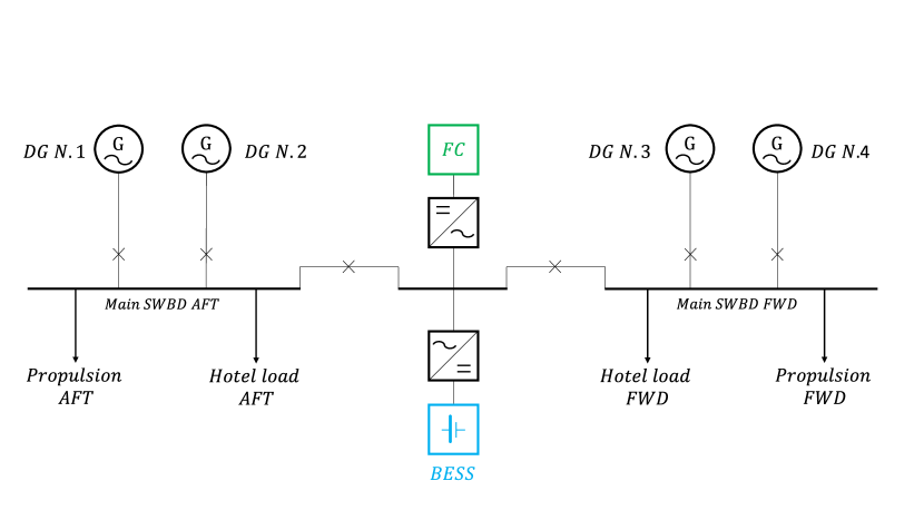
Figure 1: System Architecture.

In an AES the main load is represented by the propulsion system, which is a function of the speed of the ship. The extra propulsive load (e.g. HVAC, galley, accommodation, etc.) is represented by the hotel load [17]. Each of these loads are evaluated in the Electric Power Load Analysis (EPLA) of the ship that are divided according to the Operating Conditions (e.g. full power, navigation, etc.) of the ship [18].

II-A DG Fuel Consumption

The DG fuel consumption is modelled by a linearized Specific Fuel Oil Consumption (SFOC) curve reported in Fig. 2. The linearization is performed in two steps: (i) fitting the real data, (ii) linearize the fitted curve.

There is a non-linear relationship between SFOC and DG’s power. Manufacturer data sheets provide SFOC values at specific power levels for the DG [19]. These data points are fitted using a polynomial regression, assuming a parabolic function between SFOC and the DG’s power, as described in [20]. Subsequently, a linearization process is applied to these fitted data.

Figure 2 shows the results of the linearization that divides the quadratic function in 10 equal intervals.

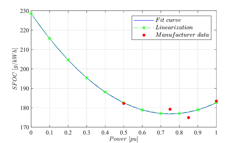
Figure 2: SFOC curve.

II-B Battery Energy Storage System

The State Of Charge (SOC) of the battery is modelled according to the following equation [21] ($\forall\;t=1:T$):

$$SOC(t+1)=SOC(t)+\biggl{(}P_{b}^{c}(t)\eta_{c}-\begin{aligned} &\left.\frac{P_{b}^{d}(t)}{\eta_{d}}\right)\frac{\Delta t}{E_{n}}\end{aligned}$$ (1)

where $E_{n}$ [$\text{\,}\mathrm{kW}\text{\,}\mathrm{h}$] is the rated energy of the battery, $P_{b}^{c}(t)$ [$\text{\,}\mathrm{kW}$] and $P_{b}^{d}(t)$ [$\text{\,}\mathrm{kW}$] are respectively the charge and discharge power variables of the battery at time $t$, $\Delta t$ is the granularity of the control and $T$ is the horizon of the optimization (notice that $t=1:T$ stands for $t=1,...,T$). The BESS consists of two main components: an energy storage unit and a conversion system. These components are represented in the model by the efficiency of the BESS, which varies for the charging ($\eta_{c}$) and discharging ($\eta_{d}$) processes of the storage system. It is assumed that the initial SOC at time $t=1$ is known and is equal to the final SOC at time $t=T$.

The BESS is composed by an energy storage and a conversion system. These components are modelled through the efficiency of the BESS which is different for the charging ($\eta_{c}$) and the discharging ($\eta_{d}$) of the storage system. It is assumed that the initial ($t=1$) SOC is known, and it is equal to the final ($t=T$) value.

II-C PEMFC and Hydrogen Storage

The specific hydrogen consumption is modeled by a linearized specific hydrogen consumption curve, as reported in Fig. 3. This curve is derived from [22] and subsequently linearized using the methodology previously described for diesel generators.

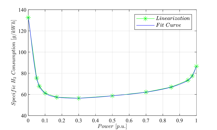
Figure 3: Specific hydrogen consumption curve.

Linearization points are selected by identifying the regions with the most significant derivative variations to minimize approximation errors.

The Level of Hydrogen (LoH) is modelled according to the following equation:

$$LoH(t+1)=LoH(t)-\frac{\dot{m}_{H_{2}}(t)\Delta t}{M_{H_{2}}}\quad\forall\;t=1:T$$ (2)

where $M_{H_{2}}$ [$\text{\,}\mathrm{t}$] is the total mass of H₂ available and $\dot{m}_{H_{2}}$ [$\text{\,}\mathrm{t}\mathrm{/}\mathrm{h}$] is the H₂ flow rate variable. The latter is derived from the specific hydrogen consumption curve shown in Fig. 3.

III Optimization Problem

The proposed methodology is based on a MILP optimization algorithm implemented in MATLAB/General Algebraic Modelling System (GAMS) environment. Several constraints are implemented in the algorithm to model the DGs, the BESS, the PEMFC and to manage the security of the system.

III-A DG and PEMFC Constraints

The linearization of the fuel flow rate ($\dot{m}_{f}$) functions is accomplished in GAMS by introducing auxiliary variables into the problem. Specifically, Special Ordered Sets of type 2 [23] (SOS2) variables ($\lambda$) have been utilized for this purpose. The piece-wise linearization is executed through the application of the following constraints (3)-(6):

$$\dot{m}_{f,i}(t)=\sum\limits_{q_{1}=1}^{n_{d}^{1}}\lambda(t,q_{1})\bar{x}(q_{1})\quad\forall\;t=1:T,\forall\;i=1:N$$ (3)

$$P_{g,i}(t)=\sum\limits_{q_{1}=1}^{n_{d}^{1}}\lambda(t,q_{1})\bar{y}(q_{1})\quad\forall\;t=1:T,\forall\;i=1:N$$ (4)

$$\sum\limits_{q_{1}=1}^{n_{d}^{1}}\lambda(t,q_{1})=1\quad\forall\;t=1:T,\forall\;i=1:N$$ (5)

$$\lambda(t,q_{1})\geq 0\quad\forall\;t=1:T,\forall\;q_{1}=1:n_{d}^{1},\forall\;i=1:N$$ (6)

where $n_{d}^{1}$ is the number of linearization intervals, $N$ is the total number of DGs and PEMFCs and $\lambda(t,q_{1})$ is an SOS2 variable that is a continuous, positive and the sum for all $q_{1}=1:n_{d}^{1}$ is always equal to one. In addition, these variables satisfy the condition that no more than two consecutive variables can be non-zero. The two parameters $\bar{x}$ and $\bar{y}$ represent the value of the linearized curve in terms of fuel flow rate variable ($\dot{m}_{f}$) and generators power variable ($P_{g,i}$), respectively.

The active power of the generating units is constrained within specific upper (7) and lower (8) set-points:

$$P_{g,i}(t)\leq c_{g}^{max}P_{g,i}^{n}z_{i}(t)\quad\forall\;i=1:N,\forall\;t=1:T$$ (7)

$$P_{g,i}(t)\geq c_{g}^{min}P_{g,i}^{n}z_{i}(t)\quad\forall\;i=1:N,\forall\;t=1:T$$ (8)

In these equations, the parameters $c_{g,min}$ and $c_{g,max}$ represent the coefficients used to calculate the minimum and maximum active power of the $i$-th generating unit, starting from $P_{g,i}^{n}$. The binary variable $z_{i}(t)$ is used to indicate the status of the $i$-th generating unit, where $z_{i}(t)=1$ signifies that the $i$-th DG is turned on at time $t$. Equation (9) models the start-up process of the DGs.

$$z_{i}(t)-z_{i}(t-1)\leq u_{i}(t)\quad\forall\;i=1:N,\forall\;t=1:T$$ (9)

The binary variable $u_{i}(t)$ is equal to 1 if the $i$-th generating unit is starting up at time $t$. Equations (10), (11) models the minimum up and the minimum downtimes of the generating units ($\forall\;i=1:N,\forall\;t=1:T$).

$$u_{i}(t)-\frac{\Delta t}{t_{min_{u},i}}\sum\limits_{u_{t}=1}^{t_{min_{u},i}/\Delta t}\begin{aligned} &{z_{i}\left(t+u_{t}\right)}\leq 0\\ \end{aligned}$$ (10)

$$u_{i}(t)+\frac{\Delta t}{t_{min_{d},i}}\sum\limits_{d_{t}=1}^{t_{min_{d},i}/\Delta t}\begin{aligned} &{z_{i}\left(t-d_{t}\right)}\leq 1\\ \end{aligned}$$ (11)

where $t_{min_{d},i}$ and $t_{min_{u},i}$ are respectively the minimum down time and the minimum up time of the $i$-th generating unit. Both of these parameters must be multiples of the simulation time-step.

Equations (12), (13) represent the ramp limits of the generating units ($\forall\;i=1:N,\forall\;t=1:T$).

$$P_{g,i}(t)-P_{g,i}(t-1)\begin{aligned} &\leq\Delta P_{r_{u},i}\\ \end{aligned}$$ (12)

$$P_{g,i}(t-1)-P_{g,i}(t)\begin{aligned} &\leq\Delta P_{r_{d,i}}\\ \end{aligned}$$ (13)

where $\Delta P_{r_{u},i}$ and $\Delta P_{r_{d},i}$ are respectively the maximum power ramp-up and ramp-down limit that a generating unit can take in a single time-step.

III-B BESS Constraints

The SOC of the BESS is limited between a minimum ($SOC_{min}$) and maximum ($SOC_{max}$) value according to the following constraints:

$$SOC_{min}\leq SOC(t)\leq SOC_{max}\quad\forall\;t=1:T$$ (14)

Equations (15), (16) represent the upper and lower bound of the charging power ($P_{b}^{c}(t)$) and discharging power ($P_{b}^{d}(t)$) for the battery at time $t$.

$$c_{c}^{min}P_{b}^{n}z_{b}^{c}(t)\leq P_{b}^{c}(t)\leq c_{c}^{max}P_{b}^{n}z_{b}^{c}(t)\quad\forall\;t=1:T$$ (15)

$$c_{d}^{min}P_{b}^{n}z_{b}^{d}(t)\leq P_{b}^{d}(t)\leq c_{d}^{max}P_{b}^{n}z_{b}^{d}(t)\quad\forall\;t=1:T$$ (16)

In these equations $c_{c,max}$,$c_{c,min}$,$c_{d,max}$ and $c_{d,min}$ represent respectively the max/min charge and the max/min discharge coefficients of the battery, while $z_{b}^{c}(t)$/$z_{b}^{d}(t)$ are two binary variable that identify if the BESS is charging/discharging at time $t$. Equation (17) models that the battery can only charge or discharge in a single time-step.

$$z_{b}^{d}(t)+z_{b}^{c}(t)=z_{b}(t)\quad\forall\;t=1:T$$ (17)

Where $z_{b}(t)$ is a binary variable that is equal to 1 if the BESS is charging or discharging a time $t$.

III-C Load balance

The generated electric power must be equal to the load demand:

$$P_{l}(t)+P_{b}^{c}(t)=\sum\limits_{i=1}^{N}P_{g,i}(t)+P_{b}^{d}(t)\quad\forall\;t=1:T$$ (18)

Here, $P_{l}$ denotes the total electric load power required by the ship, comprising both hotel load and propulsive power. The propulsive power is associated with the ship’s speed and follows a well-known cubic relationship. The modeling of this relationship incorporates the use of SOS2 variables. The constraints used are similar to those described in Section III-A for the fuel flow rate. The parameters $\bar{x}$ and $\bar{y}$ represent the values of the linearized curve in terms of Speed Over Ground (SOG) and propulsive power, respectively. A soft constraint is modelled for the SOG variable:

$$SOG_{u}(t)\leq SOG(t)\leq SOG_{l}(t)\quad\forall\;t=1:T$$ (19)

where $SOG_{u}$ and $SOG_{l}$ represent the upper and lower limits within which the ship’s speed can vary from the input value. This constraint is designed to allow for the adjustment of the ship’s speed and, consequently, the propulsive load during navigation, with the aim of identifying conditions that result in lower specific costs.

Equation (20) models the conservation of the distance traveled by the ship, maintaining it consistent with the input value provided to the algorithm.

$$\sum\limits_{t=1}^{T_{p}}SOG(t)\Delta t=D_{p}$$ (20)

where $D_{p}$ is the total distance travelled by the ship in each operating condition.

III-D Security Constraints

As introduced in Section I, the IACS requires that if one of the generating units fail, the remaining units must have the capability to prevent a blackout. This means that at least 2 generating units must be in service at all time instants $t$ to meet the electrical load.

Auxiliary variables are implemented in order to model the security constraints. Firstly, it is necessary to identify which of the $n_{g}$ generating units (DGs and BESS) are on. The PEMFC is not included in the security constraints.

There exist $n_{c}$ combinations, without repetition, of class $k$ where $k$ is greater than or equal to 2, involving generating units that are actively supplying power. For example, if there are a total of 3 units, there are 4 possible combinations of at least 2 units that are in service

It is possible to calculate this number using the binomial coefficient $C(n_{g},k)$ for each $k$ class and then sum all the coefficient where $n_{g}=N+1$ ($N$ generating unit and the battery).

Thus, in the above mentioned example, since at least 2 units must be on line, the combinations are:

$$n_{c}=\sum\limits_{k\geq 2}C(n_{g},k)=\binom{3}{2}+\binom{3}{3}=$$ (21)

$$=\frac{3!}{2!(3-2)!}+\frac{3!}{3!(3-3)!}=4$$

The first binary auxiliary variable is represented as $s_{j}(t)$. If the $j$-th combination of generators is active, then $s_{j}(t)=1$. Since at any given time $t$ only one combination can be active, the following equation models this constraint:

$$\sum\limits_{j=1}^{n_{c}}s_{j}(t)=1\quad\forall\;t=1:T$$ (22)

The second auxiliary variable ($f_{j}(t)$, integer) allows counting the units that are actively supplying power for each $j$-th combination:

$$\sum\limits_{r=1}^{n_{j}}z_{g,r}(t)=f_{j}(t)\quad\forall\;j=1:n_{c},\forall\;t=1:T$$ (23)

where the binary variable $z_{g,r}(t)$ is equal to 1 if $r$-th unit is on at time $t$ and $n_{j}$ is an integer parameter that represents the number of generating units for the $j$-th combination.

The inequality (24) links the variable $s_{j}(t)$ with $f_{j}(t)$ ensuring that when $s_{j}(t)=1$ then $f_{j}(t)=n_{j}$.

$$f_{j}(t)\geq n_{j}s_{j}(t)\quad\forall\;j=1:n_{c},\forall\;t=1:T$$ (24)

As requested by the standard, the following constraint ensures that, following the loss of a generating unit (the $r$-th in (25)), the remaining $n_{j}-1$ are able to provide the total electric power load ($\forall\;j=1:n_{c},\forall\;r=1:n_{j},\forall\;t=1:T$):

$$\delta_{j}(t)\leq\sum\limits_{h=1,h\neq r}^{n_{j}-1}\alpha_{g,h}P_{g,h}^{n}$$ (25)

where $\delta_{j}(t)$ is a continuous linear variable that allows to linearize the product between the integer variable $s_{j}(t)$ and the continuous variable $P_{l}(t)$, $\alpha_{g,h}$ represents the overload working limit that the $h$-th generator can guarantee in the event of an emergency for a short period.

Equations (26) – (27) are used to link the variable $P_{l}$ with $n_{c}$ combinations ($\forall\;j=1:n_{c},\forall\;t=1:T$).

$$0\leq\delta_{j}(t)\leq P_{l}(t)$$ (26)

$$P_{l}(t)+M\left(s_{j}(t)-1\right)\leq\delta_{j}(t)\leq s_{j}(t)M$$ (27)

These two last inequalities are characterized by the $M$ parameter. It models the so called Big M method in order to modify the constraints according to the activation of the $j$-th combination.

Equation (28) models that a generating unit can provide a maximum instantaneous load step in case of emergency ($\forall\;j=1:n_{c},\forall\;r=1:n_{j},\forall\;t=1:T$).

$$P_{g,r}(t)\leq\sum\limits_{h=1,h\neq r}^{n_{j}-1}\beta_{g,h}P_{g,h}^{n}+M(1-s_{j}(t))$$ (28)

Where $\beta_{g,w}$ represents the instantaneous variation of power of the, the variable $P_{g,r}(t)$ represents the power supplied by the $r$-th unit at time $t$.

Finally, equation (29) takes into account that in case of an emergency, each unit is able to provide the maximum load step ($\forall\;j=1:n_{c},\forall\;r=1:n_{j},\forall\;t=1:T$).

$$P_{g,r}(t)\leq(\alpha_{g,r}\leq\beta_{g,r})P_{g,r}^{n}+M(1-s_{j}(t))$$ (29)

In these two last inequalities the Big M parameter it is used to active or deactivate the constraint. In fact, when $s_{j}(t)=0$ the constraint is always satisfied since the term $M(1-s_{j}(t))$ is negative, and it is dominants to the other contribution (e.g. $M=10^{9}$).

III-E Carbon Intensity Indicator

The CII is a measure of a ship’s energy efficiency. Since January 2023, it has become mandatory for ships above 5000 Gross Tonnage (GT) [24]. The CII can be written as follows [25]:

$$CII(t)=\frac{\sum\limits_{l=1}^{t}gCO_{2}(t)}{GT\sum\limits_{l=1}^{t}D_{t}(t)}\quad\forall\;t=1:T$$ (30)

where $gCO_{2}$ is the CO₂ emitted in grams, and $D_{t}$ are the total nautical miles travelled. To linearize equation (30), it is necessary to perform a transformation using auxiliary variables. Equations (31)-(37) perform this transformation:

$$\sum\limits_{l=1}^{t}gCO_{2}(l)=u_{1}^{2}(t)-u_{2}^{2}(t)\quad\forall\;t=1:T$$ (31)

$$u_{1}(t)=\frac{1}{2}(CII(t)+GT\sum\limits_{l=1}^{t}D_{t}(l))\quad\forall\;t=1:T$$ (32)

$$u_{2}(t)=\frac{1}{2}(CII(t)-GT\sum\limits_{l=1}^{t}D_{t}(l))\quad\forall\;t=1:T$$ (33)

$$u_{1}^{2}(t)=\sum\limits_{q_{2}=1}^{n_{s}}\lambda_{2}(t,q_{2})\bar{u}_{1}(q_{2})\quad\forall\;t=1:T$$ (34)

$$u_{2}^{2}(t)=\sum\limits_{q_{2}=1}^{n_{s}}\lambda_{2}(t,q_{2})\bar{u}_{2}(q_{2})\quad\forall\;t=1:T)$$ (35)

$$\sum\limits_{q_{2}=1}^{n_{d}^{2}}\lambda_{2}(t,q_{2})=1\quad\forall\;t=1:T$$ (36)

$$\lambda_{2}(t,q_{2})\geq 0\quad\forall\;t=1:T,\forall\;q_{2}=1:n_{d}^{2}$$ (37)

where the variables $u_{1}^{2}$ and $u_{2}^{2}$ are linearised using the SOS2 variables as seen above in Section III-A. Equation (37) models that the achieved CII must not exceed a specified threshold value.

$$CII(t)\leq CII_{max}\quad\forall\;t=1:T$$ (38)

where $CII_{max}$ is the maximum allowable CII during the simulation.

III-F Objective Function

The objective function is formulated as:

$$\min\sum\limits_{t=1}^{T}\left(\sum\limits_{i=1}^{N}\dot{m}_{f,i}(t)\Bigl{(}c_{f}+e_{f}c_{CO_{2}}\Bigl{)}+c_{H_{2}}\dot{m}_{H_{2}}(t)+\right.$$ (39)

$$+c_{i}u_{i}(t)+c_{b}\Bigl{(}1-SOC(t)\Bigl{)}\Biggl{)}\Delta t$$

where $\dot{m}_{f,i}(t)$ is the fuel flow rate of $i$-th DG, $c_{f}$ is the cost of the fuel [$\text{\,}\mathrm{\text{€}}\text{/}\mathrm{kg}$], $e_{f}$ is the emission factor of CO₂, $c_{CO_{2}}$ is the cost of CO₂ [$\text{\,}\mathrm{\text{€}}\text{/}\mathrm{kg}$], $c_{H_{2}}$ is the cost of the hydrogen [$\text{\,}\mathrm{\text{€}}\text{/}\mathrm{kg}$], $c_{i}$ represents the start-up cost of the $i$-th generator and $c_{b}$ is the cost associated with the Depth Of Discharge (DOD) of the battery ($1-SOC(t)$). The optimization algorithm minimizes the total cost [$\text{\,}\mathrm{\text{€}}$], which is composed of three parts: the cost of fuel and hydrogen, the start-up cost, and the cost related to battery degradation. The latter accounts for DOD and, therefore, considers battery degradation aspects [26]. The term $c_{b}$ assigns a cost to battery management

IV Simulations and Results Analysis

The proposed algorithm has been validated through the simulation of a shipboard microgrid consisting of four DGs, a PEMFC and a BESS (see Fig.1). The rated parameters of each power source are collected in Table I.

Since the ship electrical load profile was not available, it was modelled by simulating a generic operating profile. The total ship load is composed by the hotel load, derived from the EPLA, and the propulsive load, which depends on the SOG ($\forall\;t=1:T$):

$$P_{l}(t)=P_{prop}\bigl{(}SOG(t,OC(t)\bigl{)}+P_{hotel}\bigl{(}OC(t)\bigl{)}$$ (40)

The SOG is simulated through a Markov Chain (MC) model derived from real data of similar ships [27]. The hotel load $P_{hotel}$ is obtained from the EPLA, with the addition of Gaussian noise having a variance of 5%. Figure 4 shows the load profile obtained through the above mentioned methodology. In this case, the granularity of the load modelling is equal to 15 min and T = 24 hour. The goal is to replicate the typical navigation of the cruise ship within a Norwegian fjord. The maximum speed variation is $2\text{\,}\mathrm{knts}$ in the Fjord OC.

The simulation parameters are listed in Table I.

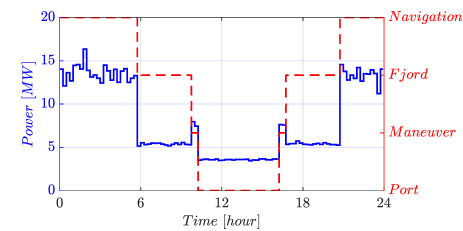
Figure 4: OC and power profile.

TABLE I: Parameters of the simulations.

Diesel Generators and Fuel Cell
Parameter	Value	Description
$P_{DG,i=1,2}^{n}$	$5.04\text{\,}\mathrm{MW}$	Rated power of i = 1,2 DG
$P_{DG,i=3,4}^{n}$	$6.72\text{\,}\mathrm{MW}$	Rated power of i = 3,4 DG
$t_{min_{u},i}$	$30\text{\,}\mathrm{min}$	Min up-time of i-th gen unit
$t_{min_{d},i}$	$30\text{\,}\mathrm{min}$	Min down-time of i-th gen unit
$c_{g,min}$	0	Min power of gen unit
$c_{g,max}$	1	Max power of gen unit
$\Delta P_{r_{u},i}$	$10\text{\,}\mathrm{MW}\text{/}\mathrm{min}$	Max gen unit power ramp-up limit
$\Delta P_{r_{d},i}$	$10\text{\,}\mathrm{MW}\text{/}\mathrm{min}$	Max gen unit power ramp-down limit
$\alpha_{g}$	1.1	Max gen unit overload in emergency
$\beta_{g}$	0.33	Max gen unit step in emergency
$c_{i}$	$200\text{\,}\mathrm{\text{€}}$	gen unit start-up cost
$c_{f}$	$0.732\text{\,}\mathrm{\text{€}}\text{/}\mathrm{kg}$	fuel cost
$c_{CO_{2}}$	$0.3\text{\,}\mathrm{\text{€}}\text{/}\mathrm{kg}$	CO2 cost [28]
$e_{f}$	3.206	Emission factor CO2 [29]
$P_{FC}^{n}$	$5\text{\,}\mathrm{MW}$	Rated power of the PEMFC
$M_{H_{2}}$	$10\text{\,}\mathrm{t}$	Mass of H2 in the storage
$c_{H_{2}}$	$5.176\text{\,}\mathrm{\text{€}}\text{/}\mathrm{kg}$	H2 cost
$n_{i}^{DG}$	10	Number of SFOC intervals curve
$n_{i}^{FC}$	11	Number of specific H2 intervals curve
Battery Energy Storage System
Parameter	Value	Description
$P_{b}^{n}$	$5\text{\,}\mathrm{MW}$	BESS nominal power
$E_{n}$	$5\text{\,}\mathrm{MWh}$	BESS nominal energy
$SOC(1)$	50%	Initial SOC of the battery
$SOC(T)$	50%	Final SOC of the battery
$SOC_{max}$	80%	Max SOC of the battery
$SOC_{min}$	20%	Min SOC of the battery
$\eta_{d}$	92%	BESS discharge efficiency
$\eta_{c}$	95%	BESS charge efficiency
$c_{c,min}$	0	Min charging C-rate
$c_{c,max}$	1	Max charging C-rate
$c_{d,min}$	0	Min discharging C-rate
$c_{d,max}$	2	Max discharging C-rate
$\alpha_{b}$	3	Max BESS overload in emergency
$c_{b}$	$5\text{\,}\mathrm{\text{€}}$	Battery utilization cost
Simulation Parameters
Parameter	Value	Description
$M$	$10^{9}$	Big M parameter
$N$	5	Number of gen unit
$D$	197.9	Total distance travelled by the ship
$CII_{max}$	13	Maximum allowable CII

The proposed power management strategy has been tested in two study cases. In the first study case (SC1), neither the BESS nor the PEMFC are considered. In the second study case (SC2), both the BESS and the PEMFC are actively involved. It’s worth noting that the Norwegian Maritime Authority mandates zero-emission navigation in the fjord. Therefore, in the second study case, the PMS is obligated to utilize only the battery and the fuel cell for the entire duration within the fjord. An exception is made for maneuvering, where security constraints ensure that power generation is met by the DGs and the battery.

Figure 5 shows the results of the optimization for the SC1, wherein the power generation is provided only by the DGs. On the other hand, Figure 6 illustrates the results obtained for SC2, where both the BESS and the PEMFC are available. The total power load, indicated in blue as $P_{load}$, represents the optimized load.

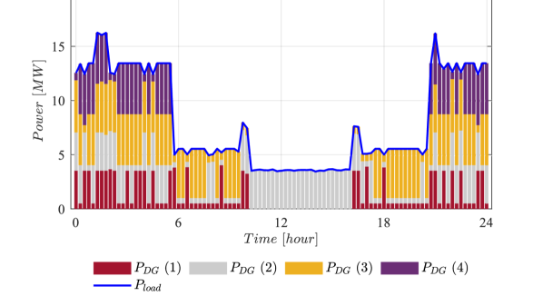
Figure 5: Simulation results, SC1. Only DGs.

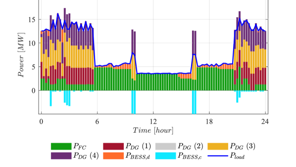
Figure 6: Simulation results, SC2. DGs, PEMFC and BESS.

The results are summarized in Table II, which reports the total cost, the amount of fuel and hydrogen required, the total CO₂ emission, the final value of the CII and the average loading factor of the DGs ($LF_{avg}$).

TABLE II: Simulations results.

SC1 - only DGs
Total Cost	Total Fuel	Total H2	CO2	CII	LFavg
$[$\text{\,}\mathrm{\text{€}}$]$	$[kg]$	$[kg]$	$[kg]$	[$g/t\cdot nm$]	[%]
61386	35415	0	113540	12	48.7
SC2 - DGs, PEMFC and BESS
Total Cost	Total Fuel	Total H2	CO2	CII	LFavg
$[$\text{\,}\mathrm{\text{€}}$]$	$[kg]$	$[kg]$	$[kg]$	[$g/t\cdot nm$]	[%]
65460	21950	5038	70371	7.4	66.8

The cost of hydrogen considered is equal to $154.29\text{\,}\mathrm{\text{€}}\mathrm{/}\mathrm{k}\mathrm{W}\mathrm{h}$. This value includes the cost of fuel plus the compressed hydrogen storage costs reported in [30]. Considering that the lower heating value of the hydrogen is equal to $33.33\text{\,}\mathrm{k}\mathrm{W}\mathrm{h}\mathrm{/}\mathrm{k}\mathrm{g}$, $c_{H_{2}}$ is equal to $5176\text{\,}\mathrm{\text{€}}\text{/}\mathrm{kg}$, as previously reported (see Table I).

The required CII for the notional cruise ship is computed according to the IMO MEPC.336(76) standard [24]:

$$CII_{required}=a\cdot GT^{-c}$$ (41)

where $a$ and $c$ are parameter defined for the ship type, for a cruise ship the value are $a=930$ and $c=0.383$. The $CII_{required}$ is equal to 15 $\text{\,}\mathrm{g}\mathrm{C}\mathrm{O}_{\mathrm{2}}\mathrm{/}\mathrm{(}\mathrm{t}\cdot\mathrm{n}\mathrm{m}\mathrm{)}$.

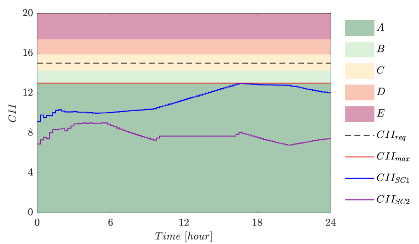
Figure 7: SC1 and SC2 CII profile comparison.

The comparison of these two study cases shows that the BESS and the PEMFC allows to reduce the CO₂ emission by 38.2% ($43\,479\text{\,}\mathrm{kg}$ of CO₂ saving with respect the SC1). In the SC2, the $LF_{avg}$ is much closer to the point of lowest specific consumption, which is approximately equal to 80% of the nominal power. It is important to highlight that both the study cases exploit the optimal control strategy. The total cost is higher in SC2. This is due to the presence of the zero-emission constraint during navigation in the Fjord. In fact, hydrogen is more expensive than VLSFO. The ranking levels are referred to the IMO MEPC.339(76) standard [31].

Figure 7 presents the comparison between the CII profile in the two study cases. In SC1, the CII reaches the maximum value imposed by the constraint, while in SC2, the CII is significantly lower.

Figure 8 illustrate the state of charge of the battery. It is worth noting that the SOC is within the selected thresholds, and that the final values of the SOC matches the initial requirements.

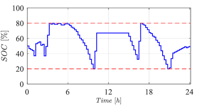
Figure 8: Battery SOC.

The algorithm has been deployed on a work station equipped with a 3.4 GHz Intel 11th-generation i7 processor and 16 GB of RAM. A three hour simulation can be solved in 43 seconds, making the algorithm suitable for real-time applications.

V Conclusions

This work proposes an optimal power management strategy for shipboard microgrids equipped with DGs, PEMFCs and BESSs. The power management algorithm is based on a MILP problem that includes the UC and the economic dispatch, to ensure a reliable power supply at minimum cost. A set of security constraints ensures to meet the IACS requirements.

Two study cases have been investigated: the first one has been used as a reference as it considers only the utilization of DGs, while the second one includes also the exploitation of a PEMFC and a BESS. The available resources considered in the second study case allow to reduce the CO₂ emission by 38.2%, and enable zero-emission for specified operating conditions.

The computational time achieved during the simulations permits the exploitation of the proposed procedure for a real time application. Future developments will be devoted to extend the algorithm through a model predictive control strategy.

References

- [1] N. Mueller, M. Westerby, and M. Nieuwenhuijsen, “Health impact assessments of shipping and port-sourced air pollution on a global scale: A scoping literature review,” Environmental Research, vol. 216, p. 114460, 2023.
- [2] Amendments to the annex of the protocol of 1978 relating to the international convention for the prevention of pollution from ships, 1973, IMO Convention MEPC 116(51), April 2004.
- [3] E. Commission, “Fit for 55—delivering the EU’s 2030 climate target on the way to climate neutrality,” Jul 2021.
- [4] J. F. Hansen and F. Wendt, “History and state of the art in commercial electric ship propulsion, integrated power systems, and future trends,” Proceedings of the IEEE, vol. 103, no. 12, pp. 2229–2242, 2015.
- [5] L. Zhu, J. Han, D. Peng, T. Wang, T. Tang, and J.-F. Charpentier, “Fuzzy logic based energy management strategy for a fuel cell/battery/ultra-capacitor hybrid ship,” in 2014 First International Conference on Green Energy ICGE, pp. 107–112.
- [6] Norwegian Maritime Authority, “Zero emissions in the world heritage fjords by 2026,” https://www.sdir.no/, 2021.
- [7] N. P. Reddy, M. K. Zadeh, C. A. Thieme, R. Skjetne, A. J. Sorensen, S. A. Aanondsen, M. Breivik, and E. Eide, “Zero-emission autonomous ferries for urban water transport: Cheaper, cleaner alternative to bridges and manned vessels,” IEEE Electrification Magazine, vol. 7, no. 4, pp. 32–45, 2019.
- [8] SC1 Main source of electrical power - Interpretations of the International Convention for the Safety of Life at Sea (SOLAS), 1974 and its Amendments, International Association of Classification Societies (IACS) Std., 1974, Rev.2, Feb. 2021.
- [9] D. Radan, T. Johansen, A. Sørensen, and A. Adnanes, “Optimization of load dependent start tables in marine power management systems with blackout prevention,” vol. 4, 12 2005.
- [10] S. Fang, Y. Xu, Z. Li, T. Zhao, and H. Wang, “Two-step multi-objective management of hybrid energy storage system in all-electric ship microgrids,” IEEE Transactions on Vehicular Technology, vol. 68, no. 4, pp. 3361–3373, 2019.
- [11] S. Mashayekh and K. L. Butler-Purry, “Security constrained power management system for the ng ips ships,” in North American Power Symposium 2010.
- [12] F. D. Kanellos, “Optimal power management with ghg emissions limitation in all-electric ship power systems comprising energy storage systems,” IEEE Transactions on Power Systems, vol. 29, no. 1, pp. 330–339, 2014.
- [13] Y. Ren, A. W.-K. Kong, and Y. Wang, “Real-time shipboard power management based on monte-carlo tree search,” IEEE Transactions on Power Systems, vol. 38, no. 4, pp. 3669–3682, 2023.
- [14] M. Rafiei, J. Boudjadar, and M.-H. Khooban, “Energy management of a zero-emission ferry boat with a fuel-cell-based hybrid energy system: Feasibility assessment,” IEEE Transactions on Industrial Electronics, vol. 68, no. 2, pp. 1739–1748, 2021.
- [15] Z. Zhang, C. Guan, and Z. Liu, “Real-time optimization energy management strategy for fuel cell hybrid ships considering power sources degradation,” IEEE Access, vol. 8, pp. 87 046–87 059, 2020.
- [16] F. D’Agostino, M. Gallo, M. Saviozzi, and F. Silvestro, “A security-constrained optimal power management algorithm for shipboard microgrids with battery energy storage system,” in 2023 IEEE International Conference on Electrical Systems for Aircraft, Railway, Ship Propulsion and Road Vehicles & International Transportation Electrification Conference (ESARS-ITEC).
- [17] A. Boveri, F. D’Agostino, P. Gualeni, D. Neroni, and F. Silvestro, “A stochastic approach to shipboard electric loads power modeling and simulation.”
- [18] N. Doerry, “Electric power load analysis,” Naval Engineers Journal, vol. 124, pp. 45–48, 12 2012.
- [19] Wärtsilä 46F, product guide, Wärtsilä, 2020.
- [20] P. Ghimire, M. Zadeh, J. Thorstensen, and E. Pedersen, “Data-driven efficiency modeling and analysis of all-electric ship powertrain: A comparison of power system architectures,” IEEE Transactions on Transportation Electrification, vol. 8, no. 2, pp. 1930–1943, 2022.
- [21] K. Hein, Y. Xu, G. Wilson, and A. K. Gupta, “Coordinated optimal voyage planning and energy management of all-electric ship with hybrid energy storage system,” IEEE Transactions on Power Systems, vol. 36, no. 3, pp. 2355–2365, 2021.
- [22] P. Wu, J. Partridge, and R. Bucknall, “Cost-effective reinforcement learning energy management for plug-in hybrid fuel cell and battery ships,” Applied Energy, vol. 275, p. 115258, 2020.
- [23] D. Bienstock and G. Zambelli, Integer Programming and Combinatorial Optimization. Wiley, 2020.
- [24] “2021 guidelines on operational carbon intensity indicators and the calculation methods (CII guidlines, g1),” International Maritime Organization, Resolution MEPC.336.
- [25] M. Gallo, D. Kaza, F. D’Agostino, M. Cavo, R. Zaccone, and F. Silvestro, “Power plant design for all-electric ships considering the assessment of carbon intensity indicator,” Energy, vol. 283, 2023.
- [26] A. Boveri, F. Silvestro, M. Molinas, and E. Skjong, “Optimal sizing of energy storage systems for shipboard applications,” IEEE Transactions on Energy Conversion, vol. 34, no. 2, pp. 801–811, 2019.
- [27] S. Massucco, G. Mosaico, M. Saviozzi, F. Silvestro, A. Fidigatti, and E. Ragaini, “An instantaneous growing stream clustering algorithm for probabilistic load modeling/profiling,” in 2020 International Conference on Probabilistic Methods Applied to Power Systems (PMAPS).
- [28] J. Hansson, S. Månsson, S. Brynolf, and M. Grahn, “Alternative marine fuels: Prospects based on multi-criteria decision analysis involving swedish stakeholders,” Biomass and Bioenergy, vol. 126, pp. 159–173, 2019.
- [29] International Maritime Organization (IMO), “Fourth greenhouse gas study 2020,” www.imo.org, 2021.
- [30] O. B. Inal, B. Zincir, and C. Deniz, “Investigation on the decarbonization of shipping: An approach to hydrogen and ammonia,” International Journal of Hydrogen Energy, vol. 47, no. 45, pp. 19 888–19 900, 2022.
- [31] IMO, 2021 guidelines on the operational carbon intensity rating of ships(CII rating guidelines, G4, MARPOL MEPC 339(76), June 2021.