Probabilistic Roadmaps for
Aerial Relay Path Planning

Abstract

Unmanned aerial vehicles (UAVs) with on-board relays can be used to establish multi-hop links that deliver high-speed connectivity beyond cell limits. This is of utmost importance e.g. in remote areas and in emergency scenarios. However, jointly designing the trajectories of multiple such flying relays is a complex task since the dimensionality of the underlying configuration space is too large to allow the direct application of traditional shortest-path methods. To bypass this difficulty, this work proposes a probabilistic roadmap algorithm based on a novel heuristic path design which is guaranteed to provide feasible paths for all UAVs under general conditions. This addresses the limitations of existing algorithms, which are typically based on non-linear optimization and, therefore, entail high complexity and cannot readily accommodate the presence of obstacles such as buildings. As corroborated via numerical experiments in an urban environment, the proposed scheme can establish a high-speed link with a user by means of just two aerial relays in a short time.

I Introduction

The large number of applications of unmanned aerial vehicles (UAV) includes extending the coverage of cellular communication networks beyond cell limits [1]. This is of interest in cases where terrestrial infrastructure is absent, as occurs in remote areas, or damaged, e.g. by a natural disaster or military attack. Depending on the implemented functionality, UAVs that serve this purpose are referred to as aerial base stations or as aerial relays.

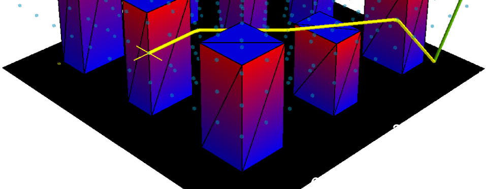
Figure 1: Trajectories of two relay UAVs obtained with the proposed PRFI algorithm. Red/blue boxes represent buildings. The yellow point on the left represents the UE location. The flight grid points are represented as blue dots. The green line is the trajectory of UAV-1, whose final position is at the green circle. The yellow line represents the trajectory of UAV-2, whose final position is the yellow cross.

The resulting research problems have attracted great interest in the last few years. Since aerial base stations typically hover at fixed positions, the problem is to determine a suitable set of locations [2]. In contrast, aerial relays typically move to address the needs of the users. A large number of works focus on the case of a single relay; see e.g. [3, 4]. However, long distances and obstructions generally require multiple relays. In this context, a substantial body of literature considers the dissemination or collection of delay-tolerant information, which is not relayed in real time but carried from one place to another by means of the movement of the UAVs; see e.g. [5]. Other works consider utilizing aerial relays to establish real-time communication links. The most common approaches involve non-linear optimization formulations over continuous variables, which include the spatial coordinates of all UAVs; see e.g. [6, 7]. Unfortunately, the resulting problems are non-convex, the solvers involve high complexity, and cannot generally accommodate no-flying zones and obstacles such as buildings. Other schemes, such as those based on mixed integer linear programs [8, 9] and the Steiner tree problem [10] also exhibit similar limitations.

Due to obstacles and other spatial constraints, the most common approaches for UAV path planning outside the literature of aerial relays are based on discretizing the airspace and applying a shortest-path algorithm on the resulting graph. This kind of approaches have been applied in the context of UAV communications e.g. to plan a path through coverage areas [11], but not to plan the trajectories of multiple aerial relays. This is because the large number of degrees of freedom renders the complexity of shortest-path algorithms prohibitive.

Inspired by the literature of motion planning for robotic manipulators, this work sidesteps this difficulty by building upon the celebrated probabilistic roadmap (PR) algorithm [12], where a shortest-path primitive is applied on a graph whose nodes are randomly generated configuration points. It is worth noting that there have been other works where PR has been applied to UAV path planning (see e.g. [13] and references therein) but never for aerial relays and, to the best of our knowledge, only in 2D or 3D spaces.

The main contribution of this work is a path planning algorithm for two relays that maintain connectivity among themselves and with a terrestrial base station (BS) and navigate through the airspace to establish a communication link with a user in an approximately minimal time. This is illustrated in Fig. 1. The algorithm can accommodate obstacles and no-fly zones, which renders it especially useful in urban scenarios, e.g. for emergency response after an earthquake. It improves upon conventional PR by drawing configuration points that rely on a heuristic waypoint sequence that can be shown to be feasible and meet the target user rate under general conditions. Besides, it is optimal in certain important cases.

After presenting the model and the problem formulation in Sec. II, the proposed algorithm is described in Sec. III. Finally, numerical experiments and conclusions are respectively presented in Secs. IV and V.

II Model and Problem Formulation

Consider a spatial region ${\color[rgb]{0,0,0}\mathcal{S}}\subset\mathbb{R}^{3}$ and let ${\color[rgb]{0,0,0}\mathcal{F}}\subset{\color[rgb]{0,0,0}\mathcal{S}}$ denote the set of points outside any building or obstacle and above the ground. For simplicity, it is assumed that if $[{\color[rgb]{0,0,0}x},{\color[rgb]{0,0,0}y},{\color[rgb]{0,0,0}z}]^{\top}\in{\color[rgb]{0,0,0}\mathcal{F}}$, then $[{\color[rgb]{0,0,0}x},{\color[rgb]{0,0,0}y},{\color[rgb]{0,0,0}z}^{\prime}]^{\top}\in{\color[rgb]{0,0,0}\mathcal{F}}$ for all ${\color[rgb]{0,0,0}z}^{\prime}\geq{\color[rgb]{0,0,0}z}$, which essentially means that the buildings or obstacles contain no holes or parts that stand out. To establish a link between a base station (BS) at location ${\color[rgb]{0,0,0}\bm{q}}_{\text{BS}}:=[{\color[rgb]{0,0,0}x}_{\text{BS}},{\color[rgb]{0,0,0}y}_{\text{BS}},{\color[rgb]{0,0,0}z}_{\text{BS}}]^{\top}\in{\color[rgb]{0,0,0}\mathcal{S}}$ and user equipment (UE) at ${\color[rgb]{0,0,0}\bm{q}}_{\text{UE}}:=[{\color[rgb]{0,0,0}x}_{\text{UE}},{\color[rgb]{0,0,0}y}_{\text{UE}},{\color[rgb]{0,0,0}z}_{\text{UE}}]^{\top}\in{\color[rgb]{0,0,0}\mathcal{S}}$, ${{\color[rgb]{0,0,0}K}}$ aerial relays are deployed. Let ${\color[rgb]{0,0,0}\bar{\mathcal{F}}}\subset{\color[rgb]{0,0,0}\mathcal{F}}$ be the set of spatial locations where the UAVs can fly, which is determined by the minimum and maximum allowed altitudes as well as no-fly zones. The position of the ${{\color[rgb]{0,0,0}k}}$-th UAV at time $t$ is represented as ${\color[rgb]{0,0,0}\bm{q}}_{{\color[rgb]{0,0,0}k}}(t)\in{\color[rgb]{0,0,0}\bar{\mathcal{F}}}$ and the positions of all UAVs at time $t$ are collected into the $3\times{{\color[rgb]{0,0,0}K}}$ matrix ${\color[rgb]{0,0,0}\bm{Q}}(t):=[{\color[rgb]{0,0,0}\bm{q}}_{1}(t),\ldots,{\color[rgb]{0,0,0}\bm{q}}_{{\color[rgb]{0,0,0}K}}(t)]$, referred to as the configuration point (CP) at time $t$. The set of all matrices ${\color[rgb]{0,0,0}\bm{Q}}(t)$ whose columns are in ${\color[rgb]{0,0,0}\bar{\mathcal{F}}}$ is the so-called configuration space (Q-space) and will be denoted as ${\color[rgb]{0,0,0}\mathcal{Q}}$. The UAVs collectively follow a trajectory ${{\color[rgb]{0,0,0}\mathcal{T}}}:=\{{\color[rgb]{0,0,0}\bm{Q}}(t),~{}t\geq 0\}$. For simplicity, they all take off at the BS, i.e. ${\color[rgb]{0,0,0}\bm{q}}_{{\color[rgb]{0,0,0}k}}(0)={\color[rgb]{0,0,0}\bm{q}}_{\text{BS}}~{}\forall{{\color[rgb]{0,0,0}k}}$.

The targeted link must convey information in both ways. In the downlink, UAV-1 relays the signal from the BS to UAV-2, UAV-2 relays the signal from UAV-1 to UAV-3, and so on until UAV-${{\color[rgb]{0,0,0}K}}$ relays the signal from UAV-$({{\color[rgb]{0,0,0}K}}-1)$ to the UE. To simplify the exposition, the focus here will be on the donwlink. Relays employ the decode-and-forward strategy with capacity-attaining codes and the interference between hops is ignored.

Besides the data to be relayed towards the UE, each UAV consumes a rate of ${\color[rgb]{0,0,0}r}_{\text{CC}}$ for command and control. This means that the achievable rate between the BS and UAV-${{\color[rgb]{0,0,0}k}}$ for a generic CP ${\color[rgb]{0,0,0}\bm{Q}}:=[{\color[rgb]{0,0,0}\bm{q}}_{1},\ldots,{\color[rgb]{0,0,0}\bm{q}}_{{\color[rgb]{0,0,0}K}}]$ can be recursively obtained as

$${\color[rgb]{0,0,0}r}_{{{\color[rgb]{0,0,0}k}}}({\color[rgb]{0,0,0}\bm{Q}})=\max(0,{\color[rgb]{0,0,0}\text{min}}\left({\color[rgb]{0,0,0}r}_{{{\color[rgb]{0,0,0}k}}-1}({\color[rgb]{0,0,0}\bm{Q}})-{\color[rgb]{0,0,0}r}_{\text{CC}},{\color[rgb]{0,0,0}c}({\color[rgb]{0,0,0}\bm{q}}_{{{\color[rgb]{0,0,0}k}}-1},{\color[rgb]{0,0,0}\bm{q}}_{{{\color[rgb]{0,0,0}k}}})\right)),$$ (1)

where ${\color[rgb]{0,0,0}c}({\color[rgb]{0,0,0}\bm{q}},{\color[rgb]{0,0,0}\bm{q}}^{\prime})$ denotes the channel capacity between a UAV at ${\color[rgb]{0,0,0}\bm{q}}$ and a UAV at ${\color[rgb]{0,0,0}\bm{q}}^{\prime}$ and ${\color[rgb]{0,0,0}r}_{1}({\color[rgb]{0,0,0}\bm{Q}})={\color[rgb]{0,0,0}c}({\color[rgb]{0,0,0}\bm{q}}_{\text{BS}},{\color[rgb]{0,0,0}\bm{q}}_{1})$. The achievable rate of the UE is

$${\color[rgb]{0,0,0}r}_{\text{UE}}({\color[rgb]{0,0,0}\bm{Q}})=\max(0,{\color[rgb]{0,0,0}\text{min}}\left({\color[rgb]{0,0,0}r}_{{{\color[rgb]{0,0,0}K}}}({\color[rgb]{0,0,0}\bm{Q}})-{\color[rgb]{0,0,0}r}_{\text{CC}},{\color[rgb]{0,0,0}c}({\color[rgb]{0,0,0}\bm{q}}_{{{\color[rgb]{0,0,0}K}}},{\color[rgb]{0,0,0}\bm{q}}_{\text{UE}})\right)).$$ (2)

Throughout the trajectory, the UAVs must have connectivity with the BS, which means that ${\color[rgb]{0,0,0}r}_{{{\color[rgb]{0,0,0}k}}}({\color[rgb]{0,0,0}\bm{Q}}(t))\geq{\color[rgb]{0,0,0}r}_{\text{CC}}~{}\forall{{\color[rgb]{0,0,0}k}},t$. Meanwhile, the UE is said to have connectivity with the BS if ${\color[rgb]{0,0,0}r}_{\text{UE}}({\color[rgb]{0,0,0}\bm{Q}})$ exceeds a given rate ${\color[rgb]{0,0,0}r}_{\text{UE}}^{\text{min}}$.

To plan the trajectory, it is necessary to know function ${\color[rgb]{0,0,0}c}({\color[rgb]{0,0,0}\bm{q}},{\color[rgb]{0,0,0}\bm{q}}^{\prime})$. In practice, one needs to resort to some approximation. For example, one can use a channel-gain map [14], a 3D terrain/city model with a ray-tracing algorithm, a line-of-sight (LOS) map, a set of bounding boxes known to contain the buildings and other obstacles, specific models for UAV channels, etc.

The problem addressed in this paper is to design a trajectory such that connectivity is established between the UE and the BS as soon as possible. Formally, given ${\color[rgb]{0,0,0}\bm{q}}_{\text{BS}}$, ${\color[rgb]{0,0,0}\bm{q}}_{\text{UE}}$, ${{\color[rgb]{0,0,0}K}}$, ${\color[rgb]{0,0,0}c}({\color[rgb]{0,0,0}\bm{q}},{\color[rgb]{0,0,0}\bm{q}}^{\prime})$, ${\color[rgb]{0,0,0}r}_{\text{CC}}$, ${\color[rgb]{0,0,0}r}_{\text{UE}}^{\text{min}}$, and the maximum UAV fly speed ${\color[rgb]{0,0,0}v}_{\text{max}}$, the problem is to solve

$$\mathop{\text{minimize}}_{{{\color[rgb]{0,0,0}\mathcal{T}}}}~{}~{} {{\color[rgb]{0,0,0}T}_{\text{c}}}({{\color[rgb]{0,0,0}\mathcal{T}}})$$ (3a)

$$\mathop{\text{s.t.}}~{}~{} {\color[rgb]{0,0,0}\bm{Q}}(t)\in{\color[rgb]{0,0,0}\mathcal{Q}}~{}\forall t$$ (3b)

$${\color[rgb]{0,0,0}\bm{Q}}(0)=[{\color[rgb]{0,0,0}\bm{q}}_{\text{BS}},\ldots,{\color[rgb]{0,0,0}\bm{q}}_{\text{BS}}]$$ (3c)

$${\color[rgb]{0,0,0}r}_{{{\color[rgb]{0,0,0}k}}}({\color[rgb]{0,0,0}\bm{Q}}(t))\geq{\color[rgb]{0,0,0}r}_{\text{CC}}~{}\forall{{\color[rgb]{0,0,0}k}},t$$ (3d)

$$\|\dot{\color[rgb]{0,0,0}\bm{q}}_{{\color[rgb]{0,0,0}k}}(t)\|\leq{\color[rgb]{0,0,0}v}_{\text{max}}~{}\forall{{\color[rgb]{0,0,0}k}},t,$$ (3e)

where ${{\color[rgb]{0,0,0}T}_{\text{c}}}({{\color[rgb]{0,0,0}\mathcal{T}}}):=\inf\{t~{}:~{}{\color[rgb]{0,0,0}r}_{\text{UE}}({\color[rgb]{0,0,0}\bm{Q}}(t))\geq{\color[rgb]{0,0,0}r}_{\text{UE}}^{\text{min}}\}$ is the connection time and $\dot{\color[rgb]{0,0,0}\bm{q}}_{{\color[rgb]{0,0,0}k}}(t)$ is the velocity vector of UAV-${{\color[rgb]{0,0,0}k}}$. Note that, consistent with the standard convention for the infimum, ${{\color[rgb]{0,0,0}T}_{\text{c}}}({{\color[rgb]{0,0,0}\mathcal{T}}})=\infty$ if ${\color[rgb]{0,0,0}r}_{\text{UE}}({\color[rgb]{0,0,0}\bm{Q}}(t))\geq{\color[rgb]{0,0,0}r}_{\text{UE}}^{\text{min}}$ does not hold for any $t$. A trajectory ${{\color[rgb]{0,0,0}\mathcal{T}}}$ is said to be valid if it is feasible and ${{\color[rgb]{0,0,0}T}_{\text{c}}}({{\color[rgb]{0,0,0}\mathcal{T}}})<\infty$. Note that a minimum distance between UAVs is not explicitly enforced but it can be readily accommodated in the proposed scheme.

III Path Planning via Probabilistic Roadmaps

Since the optimization variable in Problem (3) is a function ${\color[rgb]{0,0,0}\bm{Q}}:\mathbb{R}_{+}\rightarrow\mathbb{R}^{3\times{{\color[rgb]{0,0,0}K}}}$, finding the exact solution to (3) will not be generally possible by numerical means. For this reason, the goal in this paper will be finding a valid trajectory with a reasonably short connection time.

More specifically, the focus will be on the case ${{\color[rgb]{0,0,0}K}}=2$ since, as shown next, this suffices to guarantee the existence of a valid trajectory under general conditions. For theoretical purposes, consider a simple channel model where the capacity ${\color[rgb]{0,0,0}c}({\color[rgb]{0,0,0}\bm{q}},{\color[rgb]{0,0,0}\bm{q}}^{\prime})$ is a decreasing function ${\color[rgb]{0,0,0}c}({{\color[rgb]{0,0,0}d}})$ of the distance ${{\color[rgb]{0,0,0}d}}=\|{\color[rgb]{0,0,0}\bm{q}}-{\color[rgb]{0,0,0}\bm{q}}^{\prime}\|$ whenever there is LOS between ${\color[rgb]{0,0,0}\bm{q}}$ and ${\color[rgb]{0,0,0}\bm{q}}^{\prime}$.

Proposition 1

prop:feasibleexists Let ${{\color[rgb]{0,0,0}h}}$ denote the height of the highest obstacle and suppose that the UAVs can fly above ${{\color[rgb]{0,0,0}h}}$. Furthermore, let ${{\color[rgb]{0,0,0}d}}:=\sqrt{({\color[rgb]{0,0,0}x}_{\text{UE}}-{\color[rgb]{0,0,0}x}_{\text{BS}})^{2}+({\color[rgb]{0,0,0}y}_{\text{UE}}-{\color[rgb]{0,0,0}y}_{\text{BS}})^{2}}$ denote the horizontal distance between the BS and the UE. If ${{\color[rgb]{0,0,0}h}}<\min({\color[rgb]{0,0,0}z}_{\text{UE}}+{\color[rgb]{0,0,0}c}^{-1}({\color[rgb]{0,0,0}r}_{\text{UE}}^{\text{min}}),{\color[rgb]{0,0,0}z}_{\text{BS}}+{\color[rgb]{0,0,0}c}^{-1}({\color[rgb]{0,0,0}r}_{\text{UE}}^{\text{min}}+2{\color[rgb]{0,0,0}r}_{\text{CC}}))$ and ${{\color[rgb]{0,0,0}d}}\leq{\color[rgb]{0,0,0}c}^{-1}({\color[rgb]{0,0,0}r}_{\text{UE}}^{\text{min}}+{\color[rgb]{0,0,0}r}_{\text{CC}})$, then there exists a valid trajectory ${{\color[rgb]{0,0,0}\mathcal{T}}}$ for Problem (3).

Proof:

Let ${\color[rgb]{0,0,0}z}=\min({\color[rgb]{0,0,0}z}_{\text{UE}}+{\color[rgb]{0,0,0}c}^{-1}({\color[rgb]{0,0,0}r}_{\text{UE}}^{\text{min}}),{\color[rgb]{0,0,0}z}_{\text{BS}}+{\color[rgb]{0,0,0}c}^{-1}({\color[rgb]{0,0,0}r}_{\text{UE}}^{\text{min}}+2{\color[rgb]{0,0,0}r}_{\text{CC}}))$. It is easy to show that if UAV-1 navigates to ${\color[rgb]{0,0,0}\bm{q}}_{1}:=[{\color[rgb]{0,0,0}x}_{\text{BS}},{\color[rgb]{0,0,0}y}_{\text{BS}},{\color[rgb]{0,0,0}z}]^{\top}$ and UAV-2 navigates first to ${\color[rgb]{0,0,0}\bm{q}}_{1}$ and then to ${\color[rgb]{0,0,0}\bm{q}}_{2}:=[{\color[rgb]{0,0,0}x}_{\text{UE}},{\color[rgb]{0,0,0}y}_{\text{UE}},{\color[rgb]{0,0,0}z}]^{\top}$, then there is LOS at all hops, ${{\color[rgb]{0,0,0}\mathcal{T}}}$ is feasible, and ${{\color[rgb]{0,0,0}T}_{\text{c}}}({{\color[rgb]{0,0,0}\mathcal{T}}})<({\color[rgb]{0,0,0}z}-{\color[rgb]{0,0,0}z}_{\text{BS}}+{{\color[rgb]{0,0,0}d}})/{\color[rgb]{0,0,0}v}_{\text{max}}$. ∎

Thus, so long as ${{\color[rgb]{0,0,0}d}}$ and ${{\color[rgb]{0,0,0}h}}$ are not too large relative to ${\color[rgb]{0,0,0}r}_{\text{UE}}^{\text{min}}$ and ${\color[rgb]{0,0,0}r}_{\text{CC}}$, a valid trajectory exists with only 2 relays.

Following standard practice in UAV path planning, both spatial and temporal discretizations will be introduced. Specifically, the flight region ${\color[rgb]{0,0,0}\bar{\mathcal{F}}}$ is discretized into a regular 3D flight grid ${{\color[rgb]{0,0,0}\bar{\mathcal{F}}}_{\text{G}}}\subset{\color[rgb]{0,0,0}\bar{\mathcal{F}}}\subset\mathbb{R}^{3}$, whose points are separated along the x, y, and z axes by ${\color[rgb]{0,0,0}\delta}_{x}$, ${\color[rgb]{0,0,0}\delta}_{y}$, and ${\color[rgb]{0,0,0}\delta}_{z}$ respectively; see Fig. 1. This spatial discretization also induces a discretization of the Q-space, which for ${{\color[rgb]{0,0,0}K}}=2$ results in a grid ${{\color[rgb]{0,0,0}\mathcal{Q}}_{\text{G}}}:={{\color[rgb]{0,0,0}\bar{\mathcal{F}}}_{\text{G}}}\times{{\color[rgb]{0,0,0}\bar{\mathcal{F}}}_{\text{G}}}$. Regarding the time-domain discretization, the trajectory ${{\color[rgb]{0,0,0}\mathcal{T}}}$ will be designed by first finding a waypoint sequence ${\color[rgb]{0,0,0}\mathcal{T}}_{\text{W}}:=\{{\color[rgb]{0,0,0}\bm{Q}}[0],\ldots,{\color[rgb]{0,0,0}\bm{Q}}[{{\color[rgb]{0,0,0}N}}-1]\}$ through the grid ${{\color[rgb]{0,0,0}\mathcal{Q}}_{\text{G}}}$.

Conventional algorithms for planning the path of a single UAV create a graph whose nodes are the points of ${{\color[rgb]{0,0,0}\bar{\mathcal{F}}}_{\text{G}}}$ and where an edge exists between two nodes if the associated points are adjacent on the grid. In a 3D grid like ${{\color[rgb]{0,0,0}\bar{\mathcal{F}}}_{\text{G}}}$, each point may have at most 26 adjacent points, which makes the application of shortest-path algorithms viable. However, the grid ${{\color[rgb]{0,0,0}\mathcal{Q}}_{\text{G}}}$ has many more points than ${{\color[rgb]{0,0,0}\bar{\mathcal{F}}}_{\text{G}}}$. For example, if ${{\color[rgb]{0,0,0}\bar{\mathcal{F}}}_{\text{G}}}$ is a (small) $10\times 10\times 10$ grid, then ${{\color[rgb]{0,0,0}\mathcal{Q}}_{\text{G}}}$ has $10^{6}$ points. Besides, since each point has $27^{2}-1=728$ adjacent points, solving Problem (3) via shortest-path algorithms is challenging.

To bypass this kind of difficulties, the seminal paper [12] proposed the PR algorithm, which consists of 3 steps: Step 1: a node set ${\color[rgb]{0,0,0}\mathcal{N}}\subset{\color[rgb]{0,0,0}\mathcal{Q}}$ with a much smaller number of nodes than ${{\color[rgb]{0,0,0}\mathcal{Q}}_{\text{G}}}$ is generated at random. Step 2: the edge set ${\color[rgb]{0,0,0}\mathcal{E}}\subset{\color[rgb]{0,0,0}\mathcal{N}}\times{\color[rgb]{0,0,0}\mathcal{N}}$ is constructed by connecting each point in ${\color[rgb]{0,0,0}\mathcal{N}}$ with its nearest neighbors. Step 3: a shortest-path algorithm is found on this graph.

Unfortunately, the complexity reduction of PR comes at a cost: the number of nodes in ${\color[rgb]{0,0,0}\mathcal{N}}$ necessary to find a feasible path may be very large. The key idea in the present paper is to apply PR to solve Problem (3) but a modification is introduced to avoid the aforementioned limitation: the node generation (sampling) in Step 1 is carried out in such a way that Step 3 can always find a valid waypoint sequence. This technique is described in Sec. III-B and is based on a heuristic path planning technique presented in Sec. III-A.

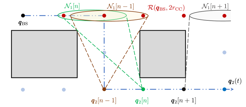
Figure 2: Top view of an example case where no path through adjacent points exists that allows UAV-1 to serve UAV-2 throughout the tentative path of the latter. At some point, UAV-2 may need to wait so that UAV-1 can gain altitude to maintain service to UAV-2. Grey boxes represent buildings and dots are grid points.

III-A Valid Path Design

This section proposes a heuristic approach that is guaranteed to find a valid path under general conditions. In many situations, this path will be nearly optimal and will typically result in a connection time much shorter than the one of the path in prop:feasibleexists; cf. Sec. IV. The idea is to first generate the path for UAV-2. Then, a path is found for UAV-1 to serve UAV-2 throughout. If this is not possible, the path of UAV-2 is lifted until it becomes possible.

Upon introducing the notation ${\color[rgb]{0,0,0}\mathcal{R}}({\color[rgb]{0,0,0}\bm{q}},{\color[rgb]{0,0,0}r}):=\{{\color[rgb]{0,0,0}\bm{q}}^{\prime}\in{{\color[rgb]{0,0,0}\bar{\mathcal{F}}}_{\text{G}}}~{}:~{}{\color[rgb]{0,0,0}c}({\color[rgb]{0,0,0}\bm{q}},{\color[rgb]{0,0,0}\bm{q}}^{\prime})\geq{\color[rgb]{0,0,0}r}\}$, it is clearly necessary (but not sufficient) that UAV-1 is in ${\color[rgb]{0,0,0}\mathcal{R}}({\color[rgb]{0,0,0}\bm{q}}_{\text{BS}},2{\color[rgb]{0,0,0}r}_{\text{CC}})$ throughout the path and in ${\color[rgb]{0,0,0}\mathcal{R}}({\color[rgb]{0,0,0}\bm{q}}_{\text{BS}},2{\color[rgb]{0,0,0}r}_{\text{CC}}+{\color[rgb]{0,0,0}r}_{\text{UE}}^{\text{min}})$ at the moment of establishing connectivity with the UE. Similarly, with notation ${\color[rgb]{0,0,0}\mathcal{R}}({\color[rgb]{0,0,0}\bm{q}},{\color[rgb]{0,0,0}r},{\color[rgb]{0,0,0}r}^{\prime}):=\{{\color[rgb]{0,0,0}\bm{q}}^{\prime\prime}\in{{\color[rgb]{0,0,0}\bar{\mathcal{F}}}_{\text{G}}}~{}|~{}\exists{\color[rgb]{0,0,0}\bm{q}}^{\prime}\in{\color[rgb]{0,0,0}\mathcal{R}}({\color[rgb]{0,0,0}\bm{q}},{\color[rgb]{0,0,0}r})~{}:~{}{\color[rgb]{0,0,0}c}({\color[rgb]{0,0,0}\bm{q}}^{\prime},{\color[rgb]{0,0,0}\bm{q}}^{\prime\prime})\geq{\color[rgb]{0,0,0}r}^{\prime}\}$, it is necessary (not sufficient) that UAV-2 is in ${\color[rgb]{0,0,0}\mathcal{N}_{2}}:={\color[rgb]{0,0,0}\mathcal{R}}({\color[rgb]{0,0,0}\bm{q}}_{\text{BS}},2{\color[rgb]{0,0,0}r}_{\text{CC}},{\color[rgb]{0,0,0}r}_{\text{CC}})$ throughout the path and in ${{\color[rgb]{0,0,0}\mathcal{D}_{2}}}:={\color[rgb]{0,0,0}\mathcal{R}}({\color[rgb]{0,0,0}\bm{q}}_{\text{BS}},2{\color[rgb]{0,0,0}r}_{\text{CC}}+{\color[rgb]{0,0,0}r}_{\text{UE}}^{\text{min}},{\color[rgb]{0,0,0}r}_{\text{CC}}+{\color[rgb]{0,0,0}r}_{\text{UE}}^{\text{min}})\cap{\color[rgb]{0,0,0}\mathcal{R}}({\color[rgb]{0,0,0}\bm{q}}_{\text{UE}},{\color[rgb]{0,0,0}r}_{\text{UE}}^{\text{min}})$ at the moment of establishing connectivity with the UE.

Tentative Path for UAV-2. The idea is to start by first planning the path of UAV-2 by finding the shortest path (e.g. via Dijkstra’s algorithm) from ${\color[rgb]{0,0,0}\bm{q}}_{\text{BS}}$ through a graph with node set ${\color[rgb]{0,0,0}\mathcal{N}_{2}}$ to the nearest point in ${{\color[rgb]{0,0,0}\mathcal{D}_{2}}}\subset{\color[rgb]{0,0,0}\mathcal{N}_{2}}$. In this graph, two nodes ${\color[rgb]{0,0,0}\bm{q}}$ and ${\color[rgb]{0,0,0}\bm{q}}^{\prime}$ are connected if they are adjacent in ${{\color[rgb]{0,0,0}\bar{\mathcal{F}}}_{\text{G}}}$, which will be denoted as $({\color[rgb]{0,0,0}\bm{q}},{\color[rgb]{0,0,0}\bm{q}}^{\prime})\in{{\color[rgb]{0,0,0}\mathcal{E}_{{{\color[rgb]{0,0,0}\bar{\mathcal{F}}}_{\text{G}}}}}}$, and the weight of an edge $({\color[rgb]{0,0,0}\bm{q}},{\color[rgb]{0,0,0}\bm{q}}^{\prime})$ is the distance $\|{\color[rgb]{0,0,0}\bm{q}}-{\color[rgb]{0,0,0}\bm{q}}^{\prime}\|$ since it is proportional to the time it takes for UAV-2 to travel from ${\color[rgb]{0,0,0}\bm{q}}$ to ${\color[rgb]{0,0,0}\bm{q}}^{\prime}$ and the objective in (3) is the connection time. This procedure produces a waypoint sequence ${\color[rgb]{0,0,0}\bm{q}}_{2}[0],{\color[rgb]{0,0,0}\bm{q}}_{2}[1],\ldots,{\color[rgb]{0,0,0}\bm{q}}_{2}[{{\color[rgb]{0,0,0}N}}-1]$.

Path for UAV-1. If a feasible waypoint sequence exists for UAV-1 that provides a sufficient rate to UAV-2 at all the waypoints ${\color[rgb]{0,0,0}\bm{q}}_{2}[0],{\color[rgb]{0,0,0}\bm{q}}_{2}[1],\ldots,{\color[rgb]{0,0,0}\bm{q}}_{2}[{{\color[rgb]{0,0,0}N}}-1]$, the combined path will not only be valid but also optimal up to the effects of the discretization. However, such a path for UAV-1 does not always exist, as seen later.

Clearly, for the combined path to be feasible, the position of UAV-1 must satisfy ${\color[rgb]{0,0,0}\bm{q}}_{1}\in{\color[rgb]{0,0,0}\mathcal{N}_{2}}[{{\color[rgb]{0,0,0}n}}]:={\color[rgb]{0,0,0}\mathcal{R}}({\color[rgb]{0,0,0}\bm{q}}_{\text{BS}},2{\color[rgb]{0,0,0}r}_{\text{CC}})\cap{\color[rgb]{0,0,0}\mathcal{R}}({\color[rgb]{0,0,0}\bm{q}}_{2}[{{\color[rgb]{0,0,0}n}}],{\color[rgb]{0,0,0}r}_{\text{CC}})$ when UAV-2 is at ${\color[rgb]{0,0,0}\bm{q}}_{2}[{{\color[rgb]{0,0,0}n}}]$. Besides, for the path to be valid, it is required that ${\color[rgb]{0,0,0}\bm{q}}_{1}\in{{\color[rgb]{0,0,0}\mathcal{D}_{1}}}:={\color[rgb]{0,0,0}\mathcal{R}}({\color[rgb]{0,0,0}\bm{q}}_{\text{BS}},2{\color[rgb]{0,0,0}r}_{\text{CC}}+{\color[rgb]{0,0,0}r}_{\text{UE}}^{\text{min}})\cap{\color[rgb]{0,0,0}\mathcal{R}}({\color[rgb]{0,0,0}\bm{q}}_{2}[{{\color[rgb]{0,0,0}N}}-1],{\color[rgb]{0,0,0}r}_{\text{CC}}+{\color[rgb]{0,0,0}r}_{\text{UE}}^{\text{min}})\subset{\color[rgb]{0,0,0}\mathcal{N}_{2}}[{{\color[rgb]{0,0,0}N}}-1]$ when UAV-2 reaches ${\color[rgb]{0,0,0}\bm{q}}_{2}[{{\color[rgb]{0,0,0}N}}-1]$. Since the set of positions where UAV-1 must be depends on ${{\color[rgb]{0,0,0}n}}$, one needs to plan a path through an extended graph. Upon letting ${\color[rgb]{0,0,0}\bar{\mathcal{N}}_{1}}[{{\color[rgb]{0,0,0}n}}]:=\{({{\color[rgb]{0,0,0}n}},{\color[rgb]{0,0,0}\bm{q}})~{}|~{}{\color[rgb]{0,0,0}\bm{q}}\in{\color[rgb]{0,0,0}\mathcal{N}_{1}}[{{\color[rgb]{0,0,0}n}}]\}$, the node set of this graph is ${\color[rgb]{0,0,0}\bar{\mathcal{N}}_{1}}:=\cup_{{{\color[rgb]{0,0,0}n}}}{\color[rgb]{0,0,0}\bar{\mathcal{N}}_{1}}[{{\color[rgb]{0,0,0}n}}]$.

As a first approach to plan the path of UAV-1, one can think of finding a path $(0,{\color[rgb]{0,0,0}\bm{q}}_{1}[0]),(1,{\color[rgb]{0,0,0}\bm{q}}_{1}[1]),\ldots,({{\color[rgb]{0,0,0}N}}-1,{\color[rgb]{0,0,0}\bm{q}}_{1}[{{\color[rgb]{0,0,0}N}}-1])$ where $({{\color[rgb]{0,0,0}n}},{\color[rgb]{0,0,0}\bm{q}}_{1}[{{\color[rgb]{0,0,0}n}}])\in{\color[rgb]{0,0,0}\bar{\mathcal{N}}_{1}}[{{\color[rgb]{0,0,0}n}}]~{}\forall{{\color[rgb]{0,0,0}n}}$, ${\color[rgb]{0,0,0}\bm{q}}_{1}[{{\color[rgb]{0,0,0}N}}-1]\in{{\color[rgb]{0,0,0}\mathcal{D}_{1}}}$, and $({\color[rgb]{0,0,0}\bm{q}}_{1}[{{\color[rgb]{0,0,0}n}}],{\color[rgb]{0,0,0}\bm{q}}_{1}[{{\color[rgb]{0,0,0}n}}+1])\in{{\color[rgb]{0,0,0}\mathcal{E}_{{{\color[rgb]{0,0,0}\bar{\mathcal{F}}}_{\text{G}}}}}}~{}\forall{{\color[rgb]{0,0,0}n}}$. If this is possible, then the sequence of waypoints ${\color[rgb]{0,0,0}\bm{Q}}[{{\color[rgb]{0,0,0}n}}]=[{\color[rgb]{0,0,0}\bm{q}}_{1}[{{\color[rgb]{0,0,0}n}}],{\color[rgb]{0,0,0}\bm{q}}_{2}[{{\color[rgb]{0,0,0}n}}]]$, ${{\color[rgb]{0,0,0}n}}=0,\ldots,{{\color[rgb]{0,0,0}N}}-1$ is, as indicated earlier, optimal. This is the case when UAV-1 can maintain connectivity to UAV-2 just by moving to adjacent locations on ${{\color[rgb]{0,0,0}\bar{\mathcal{F}}}_{\text{G}}}$. However, this may not be the case: sometimes UAV-1 may need to perform multiple steps through adjacent locations on ${{\color[rgb]{0,0,0}\bar{\mathcal{F}}}_{\text{G}}}$ to fly around obstacles in order to guarantee connectivity to UAV-2; see Fig. 2. In other words, UAV-2 needs to wait at a certain waypoint until UAV-1 adopts a suitable location. Formally, this means that the path for UAV-1 is of the form $({{\color[rgb]{0,0,0}n}}_{0},{\color[rgb]{0,0,0}\bm{q}}_{1}[0]),({{\color[rgb]{0,0,0}n}}_{1},{\color[rgb]{0,0,0}\bm{q}}_{1}[1]),\ldots,({{\color[rgb]{0,0,0}n}}_{{{\color[rgb]{0,0,0}\tilde{N}}}-1},{\color[rgb]{0,0,0}\bm{q}}_{1}[{{\color[rgb]{0,0,0}\tilde{N}}}-1])$ for some ${{\color[rgb]{0,0,0}\tilde{N}}}$, where $({{\color[rgb]{0,0,0}n}}_{{\color[rgb]{0,0,0}i}},{\color[rgb]{0,0,0}\bm{q}}_{1}[{{\color[rgb]{0,0,0}i}}])\in{\color[rgb]{0,0,0}\bar{\mathcal{N}}_{1}}[{{{\color[rgb]{0,0,0}n}}_{{\color[rgb]{0,0,0}i}}}]$, ${{\color[rgb]{0,0,0}n}}_{0}=0$, ${\color[rgb]{0,0,0}\bm{q}}_{1}[{{\color[rgb]{0,0,0}\tilde{N}}}-1]\in{{\color[rgb]{0,0,0}\mathcal{D}_{1}}}$, ${{\color[rgb]{0,0,0}n}}_{{{\color[rgb]{0,0,0}i}}-1}\leq{{\color[rgb]{0,0,0}n}}_{{{\color[rgb]{0,0,0}i}}}\leq{{\color[rgb]{0,0,0}n}}_{{{\color[rgb]{0,0,0}i}}-1}+1$, and $({\color[rgb]{0,0,0}\bm{q}}_{1}[{{\color[rgb]{0,0,0}i}}],{\color[rgb]{0,0,0}\bm{q}}_{1}[{{\color[rgb]{0,0,0}i}}+1])\in{{\color[rgb]{0,0,0}\mathcal{E}_{{{\color[rgb]{0,0,0}\bar{\mathcal{F}}}_{\text{G}}}}}}$ for all ${{\color[rgb]{0,0,0}i}}$. The corresponding sequence of waypoints for UAV-2 will be ${\color[rgb]{0,0,0}\bm{q}}_{2}[{{\color[rgb]{0,0,0}n}}_{0}],{\color[rgb]{0,0,0}\bm{q}}_{2}[{{\color[rgb]{0,0,0}n}}_{1}],\ldots,{\color[rgb]{0,0,0}\bm{q}}_{2}[{{\color[rgb]{0,0,0}n}}_{{{\color[rgb]{0,0,0}\tilde{N}}}-1}]$, that is, UAV-2 waits at ${\color[rgb]{0,0,0}\bm{q}}_{2}[{{\color[rgb]{0,0,0}n}}_{{\color[rgb]{0,0,0}i}}]$ whenever ${{\color[rgb]{0,0,0}n}}_{{{\color[rgb]{0,0,0}i}}}={{\color[rgb]{0,0,0}n}}_{{{\color[rgb]{0,0,0}i}}+1}$.

The weights of the edges in the extended (directed) graph can be selected as

$${{\color[rgb]{0,0,0}w}}\left(({{\color[rgb]{0,0,0}n}},{\color[rgb]{0,0,0}\bm{q}}),({{\color[rgb]{0,0,0}n}}^{\prime},{\color[rgb]{0,0,0}\bm{q}}^{\prime})\right)=\begin{cases}\|{\color[rgb]{0,0,0}\bm{q}}-{\color[rgb]{0,0,0}\bm{q}}^{\prime}\|&\text{ if }({\color[rgb]{0,0,0}\bm{q}},{\color[rgb]{0,0,0}\bm{q}}^{\prime})\in{{\color[rgb]{0,0,0}\mathcal{E}_{{{\color[rgb]{0,0,0}\bar{\mathcal{F}}}_{\text{G}}}}}}\\ &~{}~{}~{}\text{and}~{}{{\color[rgb]{0,0,0}n}}\leq{{\color[rgb]{0,0,0}n}}^{\prime}\leq{{\color[rgb]{0,0,0}n}}+1,\\ \infty&\text{ otherwise,}\end{cases}$$ (4)

where an infinite weight indicates that the corresponding nodes are not connected.

In certain cases, it may happen that no path can be found in the extended graph. To remedy this, one can lift the tentative path of UAV-2. To this end, let ${{\color[rgb]{0,0,0}h}}_{\text{max}}$ be the height of the lowest grid level that is higher than all buildings. The path ${\color[rgb]{0,0,0}\bm{q}}_{2}[0],{\color[rgb]{0,0,0}\bm{q}}_{2}[1],\ldots,{\color[rgb]{0,0,0}\bm{q}}_{2}[{{\color[rgb]{0,0,0}N}}-1]$ can be first replaced with ${{\color[rgb]{0,0,0}L}}({\color[rgb]{0,0,0}\bm{q}}_{2}[0]),{{\color[rgb]{0,0,0}L}}({\color[rgb]{0,0,0}\bm{q}}_{2}[1]),\ldots,{{\color[rgb]{0,0,0}L}}({\color[rgb]{0,0,0}\bm{q}}_{2}[{{\color[rgb]{0,0,0}N}}-1])$, where ${{\color[rgb]{0,0,0}L}}({\color[rgb]{0,0,0}\bm{q}})={\color[rgb]{0,0,0}\bm{q}}+[0,0,{\color[rgb]{0,0,0}\delta}_{\text{z}}]^{\top}$ if $[0,0,1]{\color[rgb]{0,0,0}\bm{q}}+{\color[rgb]{0,0,0}\delta}_{\text{z}}\leq{{\color[rgb]{0,0,0}h}}_{\text{max}}$ and ${{\color[rgb]{0,0,0}L}}({\color[rgb]{0,0,0}\bm{q}})={\color[rgb]{0,0,0}\bm{q}}$ otherwise. Next, the starting location is appended at the beginning if ${\color[rgb]{0,0,0}\bm{q}}_{2}[0]\neq{{\color[rgb]{0,0,0}L}}({\color[rgb]{0,0,0}\bm{q}}_{2}[0])$. Similarly, the end location is appended at the end if ${{\color[rgb]{0,0,0}L}}({\color[rgb]{0,0,0}\bm{q}}_{2}[{{\color[rgb]{0,0,0}N}}-1])\neq{\color[rgb]{0,0,0}\bm{q}}_{2}[{{\color[rgb]{0,0,0}N}}-1]$. This yields the lifted path ${\color[rgb]{0,0,0}\bm{q}}_{2}[0],{{\color[rgb]{0,0,0}L}}({\color[rgb]{0,0,0}\bm{q}}_{2}[0]),{{\color[rgb]{0,0,0}L}}({\color[rgb]{0,0,0}\bm{q}}_{2}[1]),\ldots,{{\color[rgb]{0,0,0}L}}({\color[rgb]{0,0,0}\bm{q}}_{2}[{{\color[rgb]{0,0,0}N}}-1]),{\color[rgb]{0,0,0}\bm{q}}_{2}[{{\color[rgb]{0,0,0}N}}-1]$.

After lifting the path of UAV-2, it is more likely that a feasible path exists for UAV-1. This procedure may need to be repeated multiple times but it will eventually succeed:

Proposition 2

Let ${\color[rgb]{0,0,0}\mathcal{S}}=[0,{{\color[rgb]{0,0,0}x}}_{\text{max}}]\times[0,{{\color[rgb]{0,0,0}y}}_{\text{max}}]\times[0,{{\color[rgb]{0,0,0}z}_{\text{max}}}]$ be the region of interest, where a sufficiently dense regular grid ${{\color[rgb]{0,0,0}\bar{\mathcal{F}}}_{\text{G}}}$ is constructed. With the channel model introduced at the beginning of Sec. III, suppose that $\sqrt{{{\color[rgb]{0,0,0}x}}_{\text{max}}^{2}+{{\color[rgb]{0,0,0}y}}_{\text{max}}^{2}}\leq{\color[rgb]{0,0,0}c}^{-1}({\color[rgb]{0,0,0}r}_{\text{CC}})$ and that ${{\color[rgb]{0,0,0}h}}_{\text{max}}\leq\sqrt{[{\color[rgb]{0,0,0}c}^{-1}(2{\color[rgb]{0,0,0}r}_{\text{CC}})]^{2}-[{\color[rgb]{0,0,0}c}^{-1}(2{\color[rgb]{0,0,0}r}_{\text{CC}}+{\color[rgb]{0,0,0}r}_{\text{UE}}^{\text{min}})]^{2}}$. If a valid path for (3) exists through waypoints in ${{\color[rgb]{0,0,0}\mathcal{Q}}_{\text{G}}}$, then the procedure described in this section yields a valid waypoint sequence ${{\color[rgb]{0,0,0}\mathcal{T}}_{\text{W}}^{\text{V}}}:=\{[{\color[rgb]{0,0,0}\bm{q}}_{1}[{{\color[rgb]{0,0,0}i}}],{\color[rgb]{0,0,0}\bm{q}}_{2}[{{\color[rgb]{0,0,0}n}}_{{\color[rgb]{0,0,0}i}}]]~{}{{\color[rgb]{0,0,0}i}}=0,\ldots,{{\color[rgb]{0,0,0}\tilde{N}}}-1\}$.

Proof:

The proof is omitted due to space limitations. ∎

Thus, if ${\color[rgb]{0,0,0}r}_{\text{UE}}^{\text{min}}$ and ${\color[rgb]{0,0,0}r}_{\text{CC}}$ are not too large relative to the size of the region, the approach in this section results in a valid path whenever such a path exists. If this condition does not hold, one can design situations where a valid path exists but the algorithm cannot find it. However, this was never observed in our experiments.

III-B Q-space Sampling for Probabilistic Roadmaps

As described earlier, the first step in PR is to randomly generate a set ${\color[rgb]{0,0,0}\mathcal{N}}$ of CPs. The sampled distribution drastically impacts the optimality and computational burden of the algorithm. In the work at hand, ${\color[rgb]{0,0,0}\mathcal{N}}$ will comprise all the CPs of the path ${{\color[rgb]{0,0,0}\mathcal{T}}_{\text{W}}^{\text{V}}}=\{{\color[rgb]{0,0,0}\bm{Q}}[0],\ldots,{\color[rgb]{0,0,0}\bm{Q}}[{{\color[rgb]{0,0,0}\tilde{N}}}-1]\}$ from Sec. III-A together with ${\color[rgb]{0,0,0}C}$ additional CPs drawn at random around these CPs and likely to be near the optimal path. Specifically, for each ${\color[rgb]{0,0,0}\bm{Q}}=[{\color[rgb]{0,0,0}\bm{q}}_{1},{\color[rgb]{0,0,0}\bm{q}}_{2}]\in{{\color[rgb]{0,0,0}\mathcal{T}}_{\text{W}}^{\text{V}}}$, the proposed sampling strategy generates $\lfloor{\color[rgb]{0,0,0}C}/{{\color[rgb]{0,0,0}\tilde{N}}}\rfloor$ configuration points ${\color[rgb]{0,0,0}{\tilde{\bm{Q}}}}=[{\color[rgb]{0,0,0}{\tilde{\bm{q}}}}_{1},{\color[rgb]{0,0,0}{\tilde{\bm{q}}}}_{2}]$ as follows.

Suppose that both ${\color[rgb]{0,0,0}\mathcal{R}}({\color[rgb]{0,0,0}\bm{q}}_{\text{BS}},2{\color[rgb]{0,0,0}r}_{\text{CC}})$ and ${\color[rgb]{0,0,0}\mathcal{R}}({\color[rgb]{0,0,0}\bm{q}}_{\text{BS}},2{\color[rgb]{0,0,0}r}_{\text{CC}},{\color[rgb]{0,0,0}r}_{\text{CC}})$ contain more than one element each. Generate ${\color[rgb]{0,0,0}{\tilde{\bm{q}}}}_{1}$ by drawing a point of ${\color[rgb]{0,0,0}\mathcal{R}}({\color[rgb]{0,0,0}\bm{q}}_{\text{BS}},2{\color[rgb]{0,0,0}r}_{\text{CC}})-\{{\color[rgb]{0,0,0}\bm{q}}_{1}\}$ with probability proportional to $1/\|{\color[rgb]{0,0,0}{\tilde{\bm{q}}}}_{1}-{\color[rgb]{0,0,0}\bm{q}}_{1}\|$. Independently of ${\color[rgb]{0,0,0}{\tilde{\bm{q}}}}_{1}$, generate ${\color[rgb]{0,0,0}{\tilde{\bm{q}}}}_{2}$ by drawing a point of ${\color[rgb]{0,0,0}\mathcal{R}}({\color[rgb]{0,0,0}\bm{q}}_{\text{BS}},2{\color[rgb]{0,0,0}r}_{\text{CC}},{\color[rgb]{0,0,0}r}_{\text{CC}})-\{{\color[rgb]{0,0,0}\bm{q}}_{2}\}$ with probability proportional to $1/\|{\color[rgb]{0,0,0}{\tilde{\bm{q}}}}_{2}-{\color[rgb]{0,0,0}\bm{q}}_{2}\|$. If ${\color[rgb]{0,0,0}{\tilde{\bm{q}}}}_{2}\notin{\color[rgb]{0,0,0}\mathcal{R}}({\color[rgb]{0,0,0}{\tilde{\bm{q}}}}_{1},{\color[rgb]{0,0,0}r}_{\text{CC}})$, another pair $({\color[rgb]{0,0,0}{\tilde{\bm{q}}}}_{1},{\color[rgb]{0,0,0}{\tilde{\bm{q}}}}_{2})$ is generated until ${\color[rgb]{0,0,0}{\tilde{\bm{q}}}}_{2}\in{\color[rgb]{0,0,0}\mathcal{R}}({\color[rgb]{0,0,0}{\tilde{\bm{q}}}}_{1},{\color[rgb]{0,0,0}r}_{\text{CC}})$, which will eventually happens as ${\color[rgb]{0,0,0}{\tilde{\bm{q}}}}_{2}\in{\color[rgb]{0,0,0}\mathcal{R}}({\color[rgb]{0,0,0}\bm{q}}_{\text{BS}},2{\color[rgb]{0,0,0}r}_{\text{CC}},{\color[rgb]{0,0,0}r}_{\text{CC}})$. In case that ${\color[rgb]{0,0,0}\mathcal{R}}({\color[rgb]{0,0,0}\bm{q}}_{\text{BS}},2{\color[rgb]{0,0,0}r}_{\text{CC}})$ and/or ${\color[rgb]{0,0,0}\mathcal{R}}({\color[rgb]{0,0,0}\bm{q}}_{\text{BS}},2{\color[rgb]{0,0,0}r}_{\text{CC}},{\color[rgb]{0,0,0}r}_{\text{CC}})$ do not contain more than one element, ${\color[rgb]{0,0,0}{\tilde{\bm{q}}}}_{1}$ and/or ${\color[rgb]{0,0,0}{\tilde{\bm{q}}}}_{2}$ are taken to be the sole element in the corresponding set.

This procedure, which is based on the distance to CPs in ${{\color[rgb]{0,0,0}\mathcal{T}}_{\text{W}}^{\text{V}}}$, ensures that many of the sampled CPs lie close to the path while others may be farther away, thereby increasing the chances for finding near-optimal trajectories in the next step.

III-C Path Planning in Q-Space

Given ${\color[rgb]{0,0,0}\mathcal{N}}$ as generated in Sec. III-B, PR constructs a nearest-neighbor graph and seeks a shortest path through it. To this end, it is necessary to define a distance (metric) between configuration points. Due to the objective in (3), the metric between ${\color[rgb]{0,0,0}\bm{Q}}=[{\color[rgb]{0,0,0}\bm{q}}_{1},{\color[rgb]{0,0,0}\bm{q}}_{2}]$ and ${\color[rgb]{0,0,0}\bm{Q}}^{\prime}=[{\color[rgb]{0,0,0}\bm{q}}^{\prime}_{1},{\color[rgb]{0,0,0}\bm{q}}^{\prime}_{2}]$ should be the time that the UAVs require to move from ${\color[rgb]{0,0,0}\bm{Q}}$ to ${\color[rgb]{0,0,0}\bm{Q}}^{\prime}$ provided that they can perform this movement without losing connectivity or abandoning ${\color[rgb]{0,0,0}\bar{\mathcal{F}}}$ and $\infty$ otherwise. In the former case, given the speed constraint (3e), the time is $\max_{{\color[rgb]{0,0,0}k}}\|{\color[rgb]{0,0,0}\bm{q}}_{{\color[rgb]{0,0,0}k}}-{\color[rgb]{0,0,0}\bm{q}}^{\prime}_{{\color[rgb]{0,0,0}k}}\|/{\color[rgb]{0,0,0}v}_{\text{max}}$, as determined by the UAV that traverses the longest distance. To check numerically whether it is possible to move from ${\color[rgb]{0,0,0}\bm{Q}}$ to ${\color[rgb]{0,0,0}\bm{Q}}^{\prime}$ in a straight line, one can check whether the rate constraints are satisfied for a certain set of points between ${\color[rgb]{0,0,0}\bm{Q}}$ and ${\color[rgb]{0,0,0}\bm{Q}}^{\prime}$.

After the nearest-neighbor graph is constructed, the shortest path is sought from the starting location $[{\color[rgb]{0,0,0}\bm{q}}_{\text{BS}},{\color[rgb]{0,0,0}\bm{q}}_{\text{BS}}]$ to any of the CPs $[{\color[rgb]{0,0,0}\bm{q}}_{1},{\color[rgb]{0,0,0}\bm{q}}_{2}]$ that satisfies ${\color[rgb]{0,0,0}\bm{q}}_{1}\in{\color[rgb]{0,0,0}\mathcal{R}}({\color[rgb]{0,0,0}\bm{q}}_{\text{BS}},2{\color[rgb]{0,0,0}r}_{\text{CC}}+{\color[rgb]{0,0,0}r}_{\text{UE}}^{\text{min}})$, ${\color[rgb]{0,0,0}\bm{q}}_{2}\in{\color[rgb]{0,0,0}\mathcal{R}}({\color[rgb]{0,0,0}\bm{q}}_{1},{\color[rgb]{0,0,0}r}_{\text{CC}}+{\color[rgb]{0,0,0}r}_{\text{UE}}^{\text{min}})$, and ${\color[rgb]{0,0,0}\bm{q}}_{2}\in{\color[rgb]{0,0,0}\mathcal{R}}({\color[rgb]{0,0,0}\bm{q}}_{\text{UE}},{\color[rgb]{0,0,0}r}_{\text{UE}}^{\text{min}})$. The waypoint sequence ${{\color[rgb]{0,0,0}\mathcal{T}}_{\text{W}}^{\text{PR}}}$ that results from application of the shortest-path algorithm will never have a greater cost that the feasible path ${{\color[rgb]{0,0,0}\mathcal{T}}_{\text{W}}^{\text{V}}}$ obtained in Sec. III-A provided that all consecutive CPs in ${{\color[rgb]{0,0,0}\mathcal{T}}_{\text{W}}^{\text{V}}}$ are connected in the PR graph, which holds so long as ${{\color[rgb]{0,0,0}\bar{\mathcal{F}}}_{\text{G}}}$ is sufficiently dense.

III-D From the Waypoint Sequence to the Trajectory

Given the waypoint sequence ${{\color[rgb]{0,0,0}\mathcal{T}}_{\text{W}}^{\text{PR}}}=\{{\color[rgb]{0,0,0}\bm{Q}}[0],\ldots,{\color[rgb]{0,0,0}\bm{Q}}[{{\color[rgb]{0,0,0}N}^{\text{PR}}}-1]\}$, it remains only to obtain the trajectory ${{{\color[rgb]{0,0,0}\mathcal{T}}}^{\text{PR}}}=\{{\color[rgb]{0,0,0}\bm{Q}}(t)~{}t\geq 0\}$. To this end, the first step is to determine the time at which the UAVs arrive at each of the waypoints ${\color[rgb]{0,0,0}\bm{Q}}[{{\color[rgb]{0,0,0}n}}]$. As indicated in Sec. III-C, the time it takes to arrive at ${\color[rgb]{0,0,0}\bm{Q}}[{{\color[rgb]{0,0,0}n}}]=[{\color[rgb]{0,0,0}\bm{q}}_{1}[{{\color[rgb]{0,0,0}n}}],{\color[rgb]{0,0,0}\bm{q}}_{2}[{{\color[rgb]{0,0,0}n}}]]$ from ${\color[rgb]{0,0,0}\bm{Q}}[{{\color[rgb]{0,0,0}n}}-1]=[{\color[rgb]{0,0,0}\bm{q}}_{1}[{{\color[rgb]{0,0,0}n}}-1],{\color[rgb]{0,0,0}\bm{q}}_{2}[{{\color[rgb]{0,0,0}n}}-1]]$ is $\max_{{\color[rgb]{0,0,0}k}}\|{\color[rgb]{0,0,0}\bm{q}}_{{\color[rgb]{0,0,0}k}}[{{\color[rgb]{0,0,0}n}}]-{\color[rgb]{0,0,0}\bm{q}}_{{\color[rgb]{0,0,0}k}}[{{\color[rgb]{0,0,0}n}}-1]\|/{\color[rgb]{0,0,0}v}_{\text{max}}$. Let $t_{{\color[rgb]{0,0,0}n}}$ represent the time at which the UAVs arrive at ${\color[rgb]{0,0,0}\bm{Q}}[{{\color[rgb]{0,0,0}n}}]$ and let $t_{0}=0$. In this case, it clearly holds that

$$t_{{\color[rgb]{0,0,0}n}}=t_{{{\color[rgb]{0,0,0}n}}-1}+\frac{\max_{{\color[rgb]{0,0,0}k}}\|{\color[rgb]{0,0,0}\bm{q}}_{{\color[rgb]{0,0,0}k}}[{{\color[rgb]{0,0,0}n}}]-{\color[rgb]{0,0,0}\bm{q}}_{{\color[rgb]{0,0,0}k}}[{{\color[rgb]{0,0,0}n}}-1]\|}{{\color[rgb]{0,0,0}v}_{\text{max}}}.$$ (5)

This provides ${\color[rgb]{0,0,0}\bm{Q}}(t_{{\color[rgb]{0,0,0}n}})$ for ${{\color[rgb]{0,0,0}n}}=0,\ldots,{{\color[rgb]{0,0,0}N}^{\text{PR}}}-1$. For $t\geq t_{{{\color[rgb]{0,0,0}N}^{\text{PR}}}-1}$, one can simply set ${\color[rgb]{0,0,0}\bm{Q}}(t)={\color[rgb]{0,0,0}\bm{Q}}(t_{{{\color[rgb]{0,0,0}N}^{\text{PR}}}-1})$. To obtain ${\color[rgb]{0,0,0}\bm{Q}}(t)$ for other values of $t$, one can simply apply an interpolation algorithm. In the experiments of Sec. IV, linear interpolation is used since it ensures that the maximum speed is never exceeded. Although the derivatives of the resulting ${\color[rgb]{0,0,0}\bm{Q}}(t)$ will be generally discontinuous at the waypoints, this is not a problem in practice since a flight controller typically requires just a sequence of waypoints, which can be readily found by resampling the interpolated ${\color[rgb]{0,0,0}\bm{Q}}(t)$ at uniform intervals.

The complete algorithm is summarized in Algorithm 1 and will be referred to as PR with feasible initialization (PRFI).

11:  Input: ${{\color[rgb]{0,0,0}\bar{\mathcal{F}}}_{\text{G}}},{\color[rgb]{0,0,0}\bm{q}}_{\text{BS}},{\color[rgb]{0,0,0}\bm{q}}_{\text{UE}},{\color[rgb]{0,0,0}r}_{\text{CC}},{\color[rgb]{0,0,0}r}_{\text{UE}}^{\text{min}},{\color[rgb]{0,0,0}c},{\color[rgb]{0,0,0}C}$.

22:   Obtain a tentative path for UAV-2.

33:   While True

• Find path for UAV-1 to serve UAV-2.

• If path found, break.

• Lift the path of UAV-2.

44:  For each ${\color[rgb]{0,0,0}\bm{Q}}\in{{\color[rgb]{0,0,0}\mathcal{T}}_{\text{W}}^{\text{V}}}$, draw $\lfloor{\color[rgb]{0,0,0}C}/{{\color[rgb]{0,0,0}\tilde{N}}}\rfloor$ CPs $\rightarrow$ ${\color[rgb]{0,0,0}\mathcal{N}}$.

55:  Construct a nearest-neighbor graph.

66:  Find the shortest path through ${\color[rgb]{0,0,0}\mathcal{N}}$.

7

87:  Obtain ${{{\color[rgb]{0,0,0}\mathcal{T}}}^{\text{PR}}}=\{{\color[rgb]{0,0,0}\bm{Q}}(t)~{}t\geq 0\}$ from ${{\color[rgb]{0,0,0}\mathcal{T}}_{\text{W}}^{\text{PR}}}$.

8:  return ${{{\color[rgb]{0,0,0}\mathcal{T}}}^{\text{PR}}}$

Algorithm 1 PR with Feasible Initialization (PRFI)

IV Numerical Experiments

This section presents numerical results that validate the efficacy and assess the performance of the proposed PRFI algorithm. The simulator and videos of some trajectories can be found at https://github.com/uiano/pr_for_relay_path_planning.

The simulation scenario consists of an urban environment of dimensions $100\times 100$ m like the one in Fig. 1. For reproducibility purposes, all buildings are set to have a height of 40 m. The minimum and maximum fly heights are respectively 10 and 70 m. The maximum UAV speed is 2.5 m/s. The carrier frequency and bandwidth of the transmitted signals are respectively 6 GHz and 20 MHz. The transmitted power of the BS and the UAVs is 17 dBm. An antenna gain of 12 dB is used at both the transmit and receive sides to simulate the beamforming gain of an antenna array. The noise power is -97 dBm. To be able to operate, each UAV needs a command-and-control rate of ${\color[rgb]{0,0,0}r}_{\text{CC}}=1$ kbps. Function ${\color[rgb]{0,0,0}c}$ is obtained using the tomographic channel model [15, 16] with an absorption of 1 dB/m inside the buildings and 0 dB/m outside the buildings. This is more favorable than a channel that requires LOS and is chosen this way to favor the benchmarks; the proposed algorithm will assume that LOS is required, which is more restrictive.

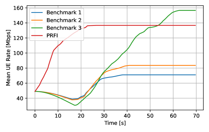
Figure 3: Expected UE rate $\mathop{\textrm{E}}\nolimits[{\color[rgb]{0,0,0}r}_{\text{UE}}({\color[rgb]{0,0,0}\bm{Q}}(t))]$ vs. time averaged across 50 MC realizations (${\color[rgb]{0,0,0}r}_{\text{UE}}^{\text{min}}$ = 100 Mbps).

Due to the presence of buildings, no algorithm in the literature that we are aware of can directly accommodate the considered simulation setup. Instead, three benchmarks will be considered: Benchmark 1 is a single UAV that takes off at ${\color[rgb]{0,0,0}\bm{q}}_{\text{BS}}$ vertically to a height of 41 m and then moves horizontally in straight line to the middle point between the BS and UE, i.e., to the point $([{\color[rgb]{0,0,0}x}_{\text{BS}},{\color[rgb]{0,0,0}y}_{\text{BS}},41]^{\top}+[{\color[rgb]{0,0,0}x}_{\text{UE}},{\color[rgb]{0,0,0}y}_{\text{UE}},41]^{\top})/2$. In Benchmark 2, two UAVs lift off at the BS to a height of 41 m above it. Then UAV-1 moves to $(2/3)[{\color[rgb]{0,0,0}x}_{\text{BS}},{\color[rgb]{0,0,0}y}_{\text{BS}},41]^{\top}+(1/3)[{\color[rgb]{0,0,0}x}_{\text{UE}},{\color[rgb]{0,0,0}y}_{\text{UE}},41]^{\top}$ whereas UAV-2 moves to $(1/3)[{\color[rgb]{0,0,0}x}_{\text{BS}},{\color[rgb]{0,0,0}y}_{\text{BS}},41]^{\top}+(2/3)[{\color[rgb]{0,0,0}x}_{\text{UE}},{\color[rgb]{0,0,0}y}_{\text{UE}},41]^{\top}$. Benchmark 3 is similar to Benchmark 2, but UAV-1 remains at $[{\color[rgb]{0,0,0}x}_{\text{BS}},{\color[rgb]{0,0,0}y}_{\text{BS}},41]^{\top}$ after lift off whereas UAV-2 flies to $[{\color[rgb]{0,0,0}x}_{\text{UE}},{\color[rgb]{0,0,0}y}_{\text{UE}},41]^{\top}$. Under the hypotheses of prop:feasibleexists, the resulting path is always feasible and yields a finite cost. All three benchmarks stop at the point of their trajectories where the UE rate is maximum. The proposed PRFI algorithm is implemented with a $12\times 12\times 8$ grid ${{\color[rgb]{0,0,0}\bar{\mathcal{F}}}_{\text{G}}}$. The number of CPs is 500 and the number of nearest neighbors is limited to 50.

In all experiments, the relevant performance metric is averaged over 50 Monte Carlo (MC) realizations in which ${\color[rgb]{0,0,0}\bm{q}}_{\text{BS}}$ and ${\color[rgb]{0,0,0}\bm{q}}_{\text{UE}}$ are randomly generated on the ground and inside ${\color[rgb]{0,0,0}\mathcal{F}}$.

Fig. 3 plots the MC estimate of the expectation $\mathop{\textrm{E}}\nolimits[{\color[rgb]{0,0,0}r}_{\text{UE}}({\color[rgb]{0,0,0}\bm{Q}}(t))]$ vs. $t$ for all compared algorithms when ${\color[rgb]{0,0,0}r}_{\text{UE}}^{\text{min}}$ = 100 Mbps. Since all UAVs start from the BS, the initial rate is the same for all algorithms. This rate is not 0 because in some MC realizations the BS and the UE may already be close to each other and possibly in LOS. Observe that the proposed algorithm attains the target rate ${\color[rgb]{0,0,0}r}_{\text{UE}}^{\text{min}}$ in just a few seconds. The rate continues increasing beyond ${\color[rgb]{0,0,0}r}_{\text{UE}}^{\text{min}}$ due to two effects: first, due to the spatial discretization, there are no grid points ${\color[rgb]{0,0,0}\bm{Q}}$ that exactly result in ${\color[rgb]{0,0,0}r}_{\text{UE}}({\color[rgb]{0,0,0}\bm{Q}})={\color[rgb]{0,0,0}r}_{\text{UE}}^{\text{min}}$. Since the algorithm needs to find destinations with ${\color[rgb]{0,0,0}r}_{\text{UE}}({\color[rgb]{0,0,0}\bm{Q}})\geq{\color[rgb]{0,0,0}r}_{\text{UE}}^{\text{min}}$, this will generally result in destinations that exceed this minimum. Second, in those MC realizations where UAV-2 needs to turn a corner to reach the UE, the rate increases suddenly. This can be seen by plotting ${\color[rgb]{0,0,0}r}_{\text{UE}}({\color[rgb]{0,0,0}\bm{Q}}(t))$ for individual MC realizations. Note also that, in accordance with prop:feasibleexists, Benchmark 3 eventually attains ${\color[rgb]{0,0,0}r}_{\text{UE}}^{\text{min}}$. Finally, it is also observed that the rate of the benchmarks initially decreases. This is due to the take-off in those realizations where there are good propagation conditions directly between the BS and UE locations.

The second experiment studies the influence of ${\color[rgb]{0,0,0}r}_{\text{UE}}^{\text{min}}$ onto the expectation of the connection time, which is the cost in Problem (3). To this end, Fig. 4 plots $\mathop{\textrm{E}}\nolimits[{{\color[rgb]{0,0,0}T}_{\text{c}}}({{\color[rgb]{0,0,0}\mathcal{T}}})|{{\color[rgb]{0,0,0}T}_{\text{c}}}({{\color[rgb]{0,0,0}\mathcal{T}}})<\infty]$ as well as the probability of failure vs. ${\color[rgb]{0,0,0}r}_{\text{UE}}^{\text{min}}$. The notation $\mathop{\textrm{E}}\nolimits[{{\color[rgb]{0,0,0}T}_{\text{c}}}({{\color[rgb]{0,0,0}\mathcal{T}}})|{{\color[rgb]{0,0,0}T}_{\text{c}}}({{\color[rgb]{0,0,0}\mathcal{T}}})<\infty]$ indicates that only those MC realizations where the ${\color[rgb]{0,0,0}r}_{\text{UE}}^{\text{min}}$ is attained are considered in the MC average. The probability of failure is defined as the fraction of MC realizations for which ${\color[rgb]{0,0,0}r}_{\text{UE}}({\color[rgb]{0,0,0}\bm{Q}}(t))<{\color[rgb]{0,0,0}r}_{\text{UE}}^{\text{min}}~{}\forall t$.

The proposed algorithm showcases a 0 probability of failure until ${\color[rgb]{0,0,0}r}_{\text{UE}}^{\text{min}}\approx 160$ Mbps and, throughout this interval, its expected connection time is much smaller than for the benchmarks. Benchmark 3 also provides a null probability of failure until ${\color[rgb]{0,0,0}r}_{\text{UE}}^{\text{min}}$ is too large, in which case the hypotheses of prop:feasibleexists no longer hold.

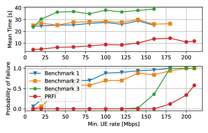
Figure 4: Mean connection time and probability of failure vs. the UE rate requirement ${\color[rgb]{0,0,0}r}_{\text{UE}}^{\text{min}}$ averaged across 50 MC realizations.

Finally, Fig. 5 plots $\mathop{\textrm{E}}\nolimits[{{\color[rgb]{0,0,0}T}_{\text{c}}}({{\color[rgb]{0,0,0}\mathcal{T}}})|{{\color[rgb]{0,0,0}T}_{\text{c}}}({{\color[rgb]{0,0,0}\mathcal{T}}})<\infty]$ and the probability of failure vs. the distance $\|{\color[rgb]{0,0,0}\bm{q}}_{\text{UE}}-{\color[rgb]{0,0,0}\bm{q}}_{\text{BS}}\|$. 50 MC realizations are generated for each considered value of $\|{\color[rgb]{0,0,0}\bm{q}}_{\text{UE}}-{\color[rgb]{0,0,0}\bm{q}}_{\text{BS}}\|$ by first drawing ${\color[rgb]{0,0,0}\bm{q}}_{\text{BS}}$ uniformly at random out of the buildings and then drawing ${\color[rgb]{0,0,0}\bm{q}}_{\text{UE}}$ on a circle of the appropriate radius and centered at ${\color[rgb]{0,0,0}\bm{q}}_{\text{BS}}$. Consistent with Fig. 4, PRFI yields a zero probability of failure throughout. At this ${\color[rgb]{0,0,0}r}_{\text{UE}}^{\text{min}}$, Benchmark 1 yields a zero connection time but this is because it only succeeds to deliver this rate in the MC realizations where the BS and UE have already good direct communication conditions.

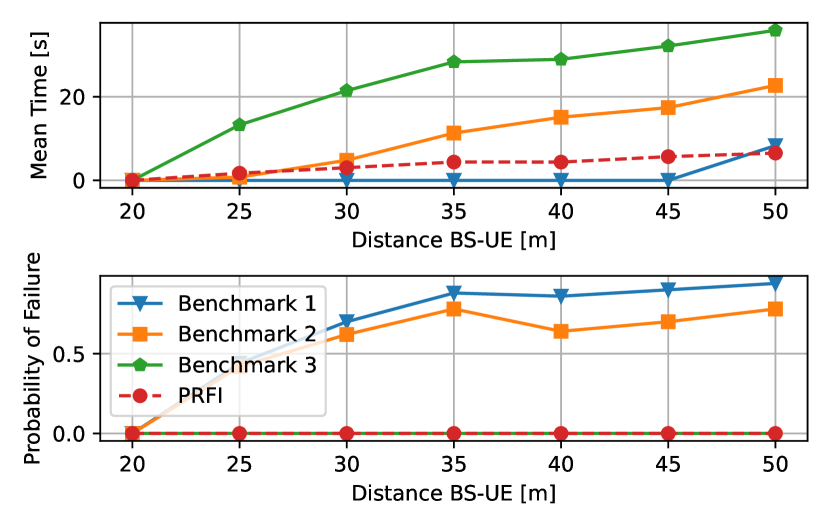
Figure 5: Mean connection time and probability of failure vs. the distance $\|{\color[rgb]{0,0,0}\bm{q}}_{\text{UE}}-{\color[rgb]{0,0,0}\bm{q}}_{\text{BS}}\|$ averaged across 50 MC realizations (${\color[rgb]{0,0,0}r}_{\text{UE}}^{\text{min}}$ = 160 Mbps).

V Conclusions

This paper proposed an algorithm to plan the paths of two aerial relays to establish a link of a given rate with a UE in an approximately minimal time. To cope with the complexity of jointly planning both paths, the PR algorithm was applied with a modification that ensures under general conditions that a valid trajectory can be found if it exists. This circumvents one of the main limitations of plain PR, which is the need for a large number of CPs to find a feasible path. Future work will develop algorithms with more than two flying relays and will investigate alternative sampling strategies.

References

• [1] P. Q. Viet and D. Romero, “Aerial base station placement: A tutorial introduction,” IEEE Commun. Magazine., vol. 60, no. 5, May 2022.
• [2] D. Romero, P. Q. Viet, and R. Shrestha, “Aerial base station placement via propagation radio maps,” arXiv preprint arXiv:2301.04966, 2023.
• [3] H. Wang, G. Ren, J. Chen, G. Ding, and Y. Yang, “Unmanned aerial vehicle-aided communications: Joint transmit power and trajectory optimization,” IEEE Wireless Commun. Lett., vol. 7, no. 4, pp. 522–525, 2018.
• [4] K. Anazawa, P. Li, T. Miyazaki, and S. Guo, “Trajectory and data planning for mobile relay to enable efficient internet access after disasters,” in IEEE Global Commun. Conf., 2015, pp. 1–6.
• [5] H. Asano, H. Okada, C. B. Naila, and M. Katayama, “Flight model using Voronoi tessellation for a delay-tolerant wireless relay network using drones,” IEEE Access, vol. 9, pp. 13064–13075, 2021.
• [6] G. Zhang, H. Yan, Y. Zeng, M. Cui, and Y. Liu, “Trajectory optimization and power allocation for multi-hop UAV relaying communications,” IEEE Access, vol. 6, pp. 48566–48576, 2018.
• [7] G. Zhang, X. Ou, M. Cui, Q. Wu, S. Ma, and W. Chen, “Cooperative UAV enabled relaying systems: Joint trajectory and transmit power optimization,” IEEE Trans. Green Commun. Netw., vol. 6, no. 1, pp. 543–557, 2022.
• [8] H. Ghazzai, M. Ben-Ghorbel, A. Kassler, and M. J. Hossain, “Trajectory optimization for cooperative dual-band UAV swarms,” in IEEE Global Commun. Conf., 2018, pp. 1–7.
• [9] J. Lee and V. Friderikos, “Trajectory planning for multiple UAVs in UAV-aided wireless relay network,” in IEEE Int. Conf. Commun., 2022, pp. 1–6.
• [10] E. Yanmaz, “Positioning aerial relays to maintain connectivity during drone team missions,” Ad Hoc Networks, vol. 128, pp. 102800, 2022.
• [11] H. Yang, J. Zhang, S. H. Song, and K. B. Lataief, “Connectivity-aware UAV path planning with aerial coverage maps,” in IEEE Wireless Commun. Netw. Conf., 2019, pp. 1–6.
• [12] L. E. Kavraki, P. Svestka, J. C. Latombe, and M. H. Overmars, “Probabilistic roadmaps for path planning in high-dimensional configuration spaces,” IEEE Trans. Robot. Autom., vol. 12, no. 4, pp. 566–580, 1996.
• [13] O. V. P. Arista, O. R. V. Barona, and R. S. Nuñez-Cruz, “Development of an efficient path planning algorithm for indoor navigation,” in Int. Conf. Electr. Eng., Comput. Sci. Automat. Control, 2021, pp. 1–6.
• [14] D. Romero and S.-J. Kim, “Radio map estimation: A data-driven approach to spectrum cartography,” IEEE Signal Process. Mag., Nov. 2022.
• [15] N. Patwari and P. Agrawal, “NeSh: a joint shadowing model for links in a multi-hop network,” in Proc. IEEE Int. Conf. Acoust., Speech, Signal Process., Las Vegas, NV, Mar. 2008, pp. 2873–2876.
• [16] N. Patwari and P. Agrawal, “Effects of correlated shadowing: Connectivity, localization, and RF tomography,” in Proc. Int. Conf. Info. Process. Sensor Networks, St. Louis, MO, Apr. 2008, pp. 82–93.