Engineering band structures and topological invariants by transformation optics

Abstract

By introducing the transformation optics method to periodic systems, we show the tunability of the band structures by comparing the results from original spaces and transformed spaces. Interestingly, we find the topological invariant Chern number will change sign when the orientation of the Brillouin zone flipped. The new platform we provided for engineering the band diagram and topological invariant might lead to the development of both transformation optics and photonic topological states.

I Introduction

Since the discovery of transformation optics (TO) [1, 2], it has become a powerful analytical tool for designing various applications such as cloak [1], field concentrator [3], optical black hole [4], and illusion optics [5]. By relating the complex transformed structure to the simple original structure, an intuitive and insightful understanding of the transformed structure can be achieved. Among all the different applications designed by TO, only a very few cover the periodic structure design [6, 7, 8]. However, due to the existence of phase factor in the Bloch function, the band diagram of the transformed structure cannot be predicted from the original structure except at $\Gamma$ point [8].

The recent discovery of photonic topological insulator [9, 10] has attracted many researchers to develop new structures and mechanisms in the photonic platforms, such as photonic spin Hall effect [11, 12, 13], photonic valley Hall effect [14, 15], high-order photonic topological insulator [16, 17], nodal lines [18, 19], and so on. Due to the bulk-boundary correspondence, edge mode could be discovered at the boundary of nontrivial photonic crystals, which are immune to local disorders and defects. Although the symmetry indicator [20, 21] and recently developed deep learning techniques [22, 23] do help in designing various photonic topological structures, a more intuitive analytic design is still waiting to be discovered.

In this paper, the TO method is applied to the period system, where we discover the precise relation between the band diagram of the transformed structure and the original structure. Furthermore, the topological invariant Chern number is calculated and compared, where we find the Chern number would change its sign if the orientation of the Brillouin zone flips. By introducing the TO method into the topology study, we can not only broaden the research scope of the TO method but also engineer the topological invariant in an insightful way, which helps deepen the understanding of the photonic topological insulator.

II Band structures engineering

As shown in Fig. 1a, we consider a square lattice (period $a=1\mathrm{m}$) with a Yttrium-Iron-Garnet (YIG) rod ($r=0.11a$) in the center. The permittivity of the YIG rod is $\epsilon=15\epsilon_{0}$ and the permeability tensor is [9]:

$$\bar{\bar{\mu}}=\begin{bmatrix}\mu&i\kappa&0\\ -i\kappa&\mu&0\\ 0&0&\mu_{0}\end{bmatrix}$$ (1)

where $\mu=14\mu_{0}$ and $\kappa=12.4\mu_{0}$. The authors show in Ref. [9] that the lowest four bands of the TM mode are well separated and nontrivial Chern numbers can be achieved in such gyromagnetic photonic crystal. If a linear coordinate transformation is applied to the square lattice as shown in Fig. 1a, the structure will transform into a diamond lattice and the shape of the Brillouin zone will also change. According to the transformation optics, the field distributions and materials are transformed in the form of [1]:

(a)

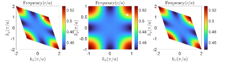
(b)

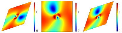
(c)

Figure 1: The band structures and eigenfield distributions under the linear transformation. (a) Center: A square lattice (period $a=1\mathrm{m}$) with a YIG rod in the center (radius $r=0.11a$, $\epsilon=15\epsilon_{0}$, $\mu=14\mu_{0}$, $\kappa=12.4\mu_{0}$). Right and left: The diamond lattice is transformed from the square lattice in the middle under the matrix $\bar{\bar{J}}_{1}$, $\bar{\bar{J}}_{2}$ respectively. (b) Band diagrams of the second band of the corresponding structures in (a). The white dots denote the locations of the eigenfields in (c). (c) $|E_{z}|$ field distributions at $k_{x}^{\prime}=0.5\pi/a$, $k_{y}^{\prime}=0.9\pi/a$ (left), $k_{x}=0.8\pi/a$, $k_{y}=0.6\pi/a$ (middle), and $k_{x}^{\prime}=0.9\pi/a$, $k_{y}^{\prime}=0.5\pi/a$ (right) of the corresponding structures in (a).

$$\bar{\bar{\epsilon}}^{\prime}=\dfrac{\bar{\bar{J}}\cdot\bar{\bar{\epsilon}}\cdot\bar{\bar{J}}^{T}}{\mathrm{det}\left(\bar{\bar{J}}\right)},\,\,\,\,\bar{\bar{\mu}}^{\prime}=\dfrac{\bar{\bar{J}}\cdot\bar{\bar{\mu}}\cdot\bar{\bar{J}}^{T}}{\mathrm{det}\left(\bar{\bar{J}}\right)}$$ (2a)

$$\vec{E}^{\prime}=\left(\bar{\bar{J}}^{T}\right)^{-1}\cdot\vec{E},\,\,\,\,\vec{H}^{\prime}=\left(\bar{\bar{J}}^{T}\right)^{-1}\cdot\vec{H}$$ (2b)

where

$$\bar{\bar{J}}=\begin{bmatrix}\dfrac{\partial x^{\prime}}{\partial x}&\dfrac{\partial x^{\prime}}{\partial y}&\dfrac{\partial x^{\prime}}{\partial z}\\ \dfrac{\partial y^{\prime}}{\partial x}&\dfrac{\partial y^{\prime}}{\partial y}&\dfrac{\partial y^{\prime}}{\partial z}\\ \dfrac{\partial z^{\prime}}{\partial x}&\dfrac{\partial z^{\prime}}{\partial y}&\dfrac{\partial z^{\prime}}{\partial z}\end{bmatrix}$$ (3)

is the Jacobian matrix of the transformation. The Bloch theorem shows the electric field should have the form $E_{z}=e^{i\vec{k}^{T}\cdot\vec{r}}u_{\vec{k}}\left(\vec{r}\right)$ where $u_{\vec{k}}\left(\vec{r}\right)$ is a periodic function and satisfies $u_{\vec{k}}\left(\vec{r}\right)=u_{\vec{k}}\left(\vec{r}+\vec{a}_{1}\right)=u_{\vec{k}}\left(\vec{r}+\vec{a}_{2}\right)$. Here, $\vec{a}_{1}=(1,0)^{T}$ and $\vec{a}_{2}=(0,1)^{T}$ are lattice vectors of the square crystal. The phase difference between point $A$ and point $B$ (see Fig. 1a) in the original space should be the same compared with the points $A^{\prime}$ and $B^{\prime}$ in the transformed space. Hence, we can conclude that:

$$e^{i\vec{k}^{\prime T}\cdot\vec{a}^{\prime}_{1}}=e^{i\vec{k}^{T}\cdot\vec{a}_{1}}$$ (4a)

$$e^{i\vec{k}^{\prime T}\cdot\vec{a}^{\prime}_{2}}=e^{i\vec{k}^{T}\cdot\vec{a}_{2}}$$ (4b)

Although Eq. (4) is not only valid in the linear transformation, we want to emphasize that not all the nonlinear transformations can match the condition shown in Eq. (4). The existence of the lattice vector $\vec{a}^{\prime}_{1}$ and $\vec{a}^{\prime}_{2}$ in the transformed space indicates two pairs of the periodic boundary should be reserved during the transformation. The line shape of the periodic boundary does not have to be straight (see Appendix A).

In our linear case, the relation between $\vec{a}_{1}$, $\vec{a}_{2}$ and $\vec{a}_{1}^{\prime}$, $\vec{a}_{2}^{\prime}$ can be expressed as:

$$\left[\vec{a}_{1}^{\prime},\vec{a}_{2}^{\prime}\right]=\begin{bmatrix}\dfrac{\partial x^{\prime}}{\partial x}&\dfrac{\partial x^{\prime}}{\partial y}\\ \dfrac{\partial y^{\prime}}{\partial x}&\dfrac{\partial y^{\prime}}{\partial y}\end{bmatrix}\left[\vec{a}_{1},\vec{a}_{2}\right]$$ (5)

Combining Eq. (4) and Eq. (5), we can figure out how the k space transforms:

$$\vec{k}=\begin{bmatrix}\dfrac{\partial x^{\prime}}{\partial x}&\dfrac{\partial y^{\prime}}{\partial x}\\ \dfrac{\partial x^{\prime}}{\partial y}&\dfrac{\partial y^{\prime}}{\partial y}\end{bmatrix}\vec{k}^{\prime}$$ (6)

As shown in Fig. 1b, the four corners of the Brillouin zone of the original square lattice are $(-\pi/a,-\pi/a)$, $(\pi/a,-\pi/a)$, $(\pi/a,\pi/a)$, and $(-\pi/a,\pi/a)$. When the transformation matrix is $\bar{\bar{J}}_{1}=\begin{bmatrix}0.75&0.25&0\\ 0.25&0.75&0\\ 0&0&1\end{bmatrix}$, we can figure out the four corners of the transformed Brillouin zone $(-\pi/a,-\pi/a)$, $(2\pi/a,-2\pi/a)$, $(\pi/a,\pi/a)$, and $(-2\pi/a,2\pi/a)$ by applying Eq. (6). Similarly, for the transformation matrix $\bar{\bar{J}}_{2}=\begin{bmatrix}0.25&0.75&0\\ 0.75&0.25&0\\ 0&0&1\end{bmatrix}$, we can find out the corners of the transformed Brillouin zone are $(-\pi/a,-\pi/a)$, $(-2\pi/a,2\pi/a)$, $(\pi/a,\pi/a)$, and $(2\pi/a,-2\pi/a)$. Although the Brillouin zones look the same under the transformation $\bar{\bar{J}}_{1}$ and $\bar{\bar{J}}_{2}$ (see Fig. 1b), the orientation has been flipped by comparing the chirality (right-handed for $\bar{\bar{J}}_{1}$ and left-handed for $\bar{\bar{J}}_{2}$) of the four corners just calculated. No matter how complicated the transformation may behave in the real space, the reaction in the k space is always a simple linear stretch or compression as shown in Eq. (6). In the middle of Fig. 1c we show the Comsol simulation result of $E_{z}$ field distribution at $k_{x}=0.8\pi/a$, $k_{y}=0.6\pi/a$. By applying Eq. (6), we can figure out the transformed $\vec{k}^{\prime}$, which are $k_{x}^{\prime}=0.9\pi/a$, $k_{y}^{\prime}=0.5\pi/a$ and $k_{x}^{\prime}=0.5\pi/a$, $k_{y}^{\prime}=0.9\pi/a$ for $\bar{\bar{J}}_{1}$, $\bar{\bar{J}}_{2}$ respectively. The transformation of the electric field in the real space satisfies the relation given in Eq. (2b). The field is compressed in the direction of $y^{\prime}=-x^{\prime}$ under the transformation $\bar{\bar{J}}_{1}$ while for $\bar{\bar{J}}_{2}$ the field is flipped along the direction of $y^{\prime}=x^{\prime}$ after the compression.

III Topological invariant engineering

Following the definition from Ref. [9], the Berry connection can be expressed as:

$$A_{x}=\iint E_{z}^{*}\epsilon_{zz}\left(\vec{r}\right)\partial_{k_{x}}E_{z}\,\mathrm{d}x\,\mathrm{d}y$$ (7a)

$$A_{y}=\iint E_{z}^{*}\epsilon_{zz}\left(\vec{r}\right)\partial_{k_{y}}E_{z}\,\mathrm{d}x\,\mathrm{d}y$$ (7b)

where the integration domain is the unit cell in real space. The Chern number is defined as:

$$C=\frac{1}{2\pi i}\iint\left(\partial_{k_{x}}A_{y}-\partial_{k_{y}}A_{x}\right)\mathrm{d}k_{x}\,\mathrm{d}k_{y}$$ (8)

The authors have shown the nontrivial Chern number in the gyromagnetic structure [9], where $C=1$ for the second band and $C=-2$ for the third band.

If we apply the time-reversal transformation to the gyromagnetic material, we will change the permeability tensor $\bar{\bar{\mu}}=\begin{bmatrix}\mu&i\kappa&0\\ -i\kappa&\mu&0\\ 0&0&\mu_{0}\end{bmatrix}$ into $\bar{\bar{\mu}}^{\prime}=\begin{bmatrix}\mu&-i\kappa&0\\ i\kappa&\mu&0\\ 0&0&\mu_{0}\end{bmatrix}$ (the permittivity of the YIG rod and the background vacuum won’t change). Obviously, the Chern number of the time-reversal transformed structure will change its sign since it is related to the sign of $\kappa$ in the permeability tensor. Interestingly, the transformation can also be explained from the perspective of TO. If we apply the Jacobian matrix $\bar{\bar{J}}=\begin{bmatrix}1&0&0\\ 0&-1&0\\ 0&0&-1\end{bmatrix}$ to the gyromagnetic permeability tensor, we can achieve the exactly same transformed permeability tensor as the time-reversal transformation will do (again, the permittivity of the YIG rod and the background vacuum won’t change). Hence, the TO shows its ability to engineer the topological invariant Chern number.

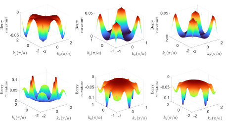
Figure 2: Berry curvatures of the original structure and the transformed structures. Top: Berry curvatures of the second band. Bottom: Berry curvatures of the third band. Middle: Original square lattice. Right and left: The diamond lattices transformed under $\bar{\bar{J}}_{1}$, $\bar{\bar{J}}_{2}$ respectively.

Through detailed derivation (see Appendix B), we discover the relation between the Chern number in the transformed space and the original space:

$$C^{\prime}\!=\mathrm{sign}\left(\mathrm{det}\left(\dfrac{\partial\left(k_{x}^{\prime},k_{y}^{\prime}\right)}{\partial\left(k_{x},k_{y}\right)}\right)\right)C$$ (9)

According to Eq. (9), we can conclude that the Chern number in the transformed space will change its sign compared with the original space when the orientation of the Brillouin zone is flipped after the transformation.

As shown in Fig. 2, the Berry curvatures of the original structure and the transformed structures are plotted. Here, the Berry curvature is the integrand in Eq. (8), which means we can achieve the Chern number by summing up the Berry curvature shown in Fig. 2. For our linear transformation $\bar{\bar{J}}_{1}$, $\bar{\bar{J}}_{2}$, by combining Eq. (6) and Eq. (9) we can get $C^{\prime}=\mathrm{sign}\left(\mathrm{det}\left(\dfrac{\partial\left(x^{\prime},y^{\prime}\right)}{\partial\left(x,y\right)}\right)\right)C$. For transformation $\bar{\bar{J}}_{1}$, since $\mathrm{det}\left(\dfrac{\partial\left(x^{\prime},y^{\prime}\right)}{\partial\left(x,y\right)}\right)>0$, the Chern number is $C^{\prime}=1$ for the second band and $C^{\prime}=-2$ for the third band, which is the same as the original structure. However, due to $\mathrm{det}\left(\dfrac{\partial\left(x^{\prime},y^{\prime}\right)}{\partial\left(x,y\right)}\right)<0$ for $\bar{\bar{J}}_{2}$, the Chern number changes its sign and turns into $C^{\prime}=-1$ for the second band and $C^{\prime}=2$ for the third band. These results can be verified by observing the distributions of the Berry curvatures as shown in Fig. 2 easily.

IV Conclusions

In the paper, we have shown that the TO method can be applied to the periodic structures to tune the band diagrams and the eigenfield distributions. Although the transformation in the real space can be nonlinear and complicated, its effect on the band diagram will always be linear. Since we assume the sign of determinant of the Jacobian matrix does not change in real space, it may constrain the ability of the TO method to engineer the topological invariant. Whether the Chern number can be tuned to a value with a different absolute value by TO is still open to be discovered.

Appendix A Curved periodic boundary

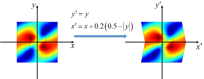
Figure 3: Transformation from a square lattice to a lattice with curved periodic boundaries. The period of the square lattice is $a=1\mathrm{m}$ and the side length is $0.4\mathrm{m}$ for the smaller square. The material is set as $\epsilon=2\epsilon_{0}$, $\mu=2\mu_{0}$ for the smaller square and it is surrounded by the vacuum. $|E_{z}|$ field distributions at $k_{x}=\pi/3$, $k_{y}=\pi/2$, and $f=0.74c/a$ are plotted for the original structure and transformed structure.

As shown in Fig. 3, a square lattice can be transformed into a lattice with curved periodic boundaries. The period of the square is $1\mathrm{m}$ and the side length of the smaller square is $0.4\mathrm{m}$. The permittivity and permeability of the smaller square are $\epsilon=2\epsilon_{0}$ and $\mu=2\mu_{0}$ respectively. The transformation matrix is $\bar{\bar{J}}=\begin{bmatrix}1&\mp 0.2&0\\ 0&1&0\\ 0&0&1\end{bmatrix}$ where ’-’ is for the domain $y>0$ and ’+’ is for the domain $y<0$. The corresponding material transformation follows the rules governed by Eq. (2a). Since the transformed lattice vectors are the same as the original lattice vectors ($\vec{a}_{1}^{\prime}=\vec{a}_{1}$, $\vec{a}_{2}^{\prime}=\vec{a}_{2}$), the k space also keeps the same $\vec{k}^{\prime}=\vec{k}$ according to the Eq. (4). The $|E_{z}|$ field distribution of the original structure is plotted at $k_{x}=\pi/3$, $k_{y}=\pi/2$, and $f=0.74c/a$ in Fig. 3. It matches to $k_{x}^{\prime}=\pi/3$, $k_{y}^{\prime}=\pi/2$, and $f^{\prime}=0.74c/a$ in the transformed space. By comparing the field distributions, we find they exactly follow the rules given in Eq. (2b). For more complicated transformed periodic boundaries, we can use the piecewise linear boundaries to approximate them and run Comsol simulations to help understand the eigenfields.

Appendix B Chern number calculation under transformation optics

Here, we will derive the Chern number of the original space and transformed space. The Berry connection in the 2D photonic crystal system can be written as [9]:

$$A_{x}=\iint E_{i}^{*}\epsilon^{ij}\partial_{k_{x}}E_{j}\,\mathrm{d}x\,\mathrm{d}y$$ (10a)

$$A_{y}=\iint E_{i}^{*}\epsilon^{ij}\partial_{k_{y}}E_{j}\,\mathrm{d}x\,\mathrm{d}y$$ (10b)

where $\epsilon^{ij}$, $E_{i}$ represent the 3 by 3 permittivity and 3 by 1 electric field in the tensor form. In our 2D case, we have $E_{1}=0,E_{2}=0,E_{3}=E_{z}$. Repeated indices $i$ and $j$ are summed over according to the Einstein summation rules. Hence, the Chern number in the original space is:

$$C = \frac{1}{2\pi i}\iint\left(\partial_{k_{x}}A_{y}-\partial_{k_{y}}A_{x}\right)\mathrm{d}k_{x}\,\mathrm{d}k_{y}$$ (11)

$$= \frac{1}{2\pi i}\iiiint(\partial_{k_{x}}E_{i}^{*}\epsilon^{ij}\partial_{k_{y}}E_{j}$$

$$- \partial_{k_{y}}E_{i}^{*}\epsilon^{ij}\partial_{k_{x}}E_{j})\mathrm{d}x\,\mathrm{d}y\,\mathrm{d}k_{x}\,\mathrm{d}k_{y}$$

We assume the electric field is normalized before transformation, which means:

$$\iint E_{i}^{*}\epsilon^{ij}E_{j}\mathrm{d}x\,\mathrm{d}y=1$$ (12)

After the transformation, the norm of the above expression changes into

$$\iint E_{i^{\prime}}^{*}\epsilon^{i^{\prime}j^{\prime}}E_{j^{\prime}}\mathrm{d}x^{\prime}\mathrm{d}y^{\prime} = \iint E_{i}^{*}J_{i^{\prime}}^{i}$$

$$\dfrac{J_{p}^{i^{\prime}}\epsilon^{pq}J_{q}^{j^{\prime}}}{\mathrm{det}\left(\dfrac{\partial\left(x^{\prime},y^{\prime},z^{\prime}\right)}{\partial\left(x,y,z\right)}\right)}J_{j^{\prime}}^{j} E_{j} \left|\mathrm{det}\left(\dfrac{\partial\left(x^{\prime},y^{\prime}\right)}{\partial\left(x,y\right)}\right)\right|\mathrm{d}x\mathrm{d}y$$ (13)

$$= \dfrac{\left|\mathrm{det}\left(\dfrac{\partial\left(x^{\prime},y^{\prime}\right)}{\partial\left(x,y\right)}\right)\right|}{\mathrm{det}\left(\dfrac{\partial\left(x^{\prime},y^{\prime},z^{\prime}\right)}{\partial\left(x,y,z\right)}\right)}$$

The summation of two Jacobian matrices can be simplified as $J^{i}_{i^{\prime}}J^{i^{\prime}}_{p}=\delta_{p}^{i}$. Also, let’s assume the transformation is linear, which means the Jacobian matrix is independent of the integration variable $x$, $y$. Then we can immediately get Eq. (13) by substituting Eq. (12) into it. However, we want to emphasize that even for some special nonlinear transformation cases, Eq. (13) can still be valid since in 2D photonic crystal the coupling between coordinates $x,y$ and $z$ is neglected. The determinant of the Jacobian matrix can be decomposed into

$$\mathrm{det}\left(\dfrac{\partial\left(x^{\prime},y^{\prime},z^{\prime}\right)}{\partial\left(x,y,z\right)}\right)=\mathrm{det}\left(\dfrac{\partial\left(x^{\prime},y^{\prime}\right)}{\partial\left(x,y\right)}\right)\dfrac{\mathrm{d}z^{\prime}}{\mathrm{d}z}$$ (14)

As long as the sign of $\mathrm{det}\left(\dfrac{\partial\left(x^{\prime},y^{\prime}\right)}{\partial\left(x,y\right)}\right)$ does not change in the whole integration area, we can still take out the term $\dfrac{\left|\mathrm{det}\left(\dfrac{\partial\left(x^{\prime},y^{\prime}\right)}{\partial\left(x,y\right)}\right)\right|}{\mathrm{det}\left(\dfrac{\partial\left(x^{\prime},y^{\prime},z^{\prime}\right)}{\partial\left(x,y,z\right)}\right)}$ and get Eq. (13). Hence, the normalized electric field after transformation can be expressed as

$$\iint\dfrac{\mathrm{det}\left(\dfrac{\partial\left(x^{\prime},y^{\prime},z^{\prime}\right)}{\partial\left(x,y,z\right)}\right)}{\left|\mathrm{det}\left(\dfrac{\partial\left(x^{\prime},y^{\prime}\right)}{\partial\left(x,y\right)}\right)\right|}E_{i^{\prime}}^{*}\epsilon^{i^{\prime}j^{\prime}}E_{j^{\prime}}\mathrm{d}x^{\prime}\mathrm{d}y^{\prime}=1$$ (15)

Similar to Eq. (10), the Berry connection defined in the transformed space is

$$A_{x}^{\prime}\!\!=\!\!\iint\dfrac{\mathrm{det}\left(\dfrac{\partial\left(x^{\prime},y^{\prime},z^{\prime}\right)}{\partial\left(x,y,z\right)}\right)}{\left|\mathrm{det}\left(\dfrac{\partial\left(x^{\prime},y^{\prime}\right)}{\partial\left(x,y\right)}\right)\right|}E_{i^{\prime}}^{*}\epsilon^{i^{\prime}j^{\prime}}\partial_{k_{x}^{\prime}}E_{j^{\prime}}\mathrm{d}x^{\prime}\mathrm{d}y^{\prime}$$ (16)

Here the normalization term $\dfrac{\mathrm{det}\left(\dfrac{\partial\left(x^{\prime},y^{\prime},z^{\prime}\right)}{\partial\left(x,y,z\right)}\right)}{\left|\mathrm{det}\left(\dfrac{\partial\left(x^{\prime},y^{\prime}\right)}{\partial\left(x,y\right)}\right)\right|}$ does not relate to variable $k_{x}^{\prime}$, which means it can be taken out from the derivative with respect to $k_{x}^{\prime}$ and put at the front of the integral term as shown in Eq. (16). Following the same procedure as Eq. (13), let’s replace the electric field $E_{j}^{\prime}$ and permittivity $\epsilon^{i^{\prime}j^{\prime}}$ in the transformed space with the electric field $E_{j}$ and permittivity $\epsilon^{ij}$ in the original space according to the transformation optics, we can easily get:

$$A_{x}^{\prime}=\iint E_{i}^{*}\epsilon^{ij}\partial_{k_{x}^{\prime}}E_{j}\,\mathrm{d}x\,\mathrm{d}y$$ (17)

Similarly,

$$A_{y}^{\prime}=\iint E_{i}^{*}\epsilon^{ij}\partial_{k_{y}^{\prime}}E_{j}\,\mathrm{d}x\,\mathrm{d}y$$ (18)

The Chern number after transformation can be calculated as

$$\!\!\!\!\!\!C^{\prime}\! = \!\frac{1}{2\pi i}\iint\left(\partial_{k_{x}^{\prime}}A_{y}^{\prime}-\partial_{k_{y}^{\prime}}A_{x}^{\prime}\right)\mathrm{d}k_{x}^{\prime}\mathrm{d}k_{y}^{\prime}\!=\!\frac{1}{2\pi i}\iiiint\!\left(\partial_{k_{x}^{\prime}}E_{i}^{*}\epsilon^{ij}\partial_{k_{y}^{\prime}}E_{j}\!-\!\partial_{k_{y}^{\prime}}E_{i}^{*}\epsilon^{ij}\partial_{k_{x}^{\prime}}E_{j}\right)\!\left|\dfrac{\partial\left(k_{x}^{\prime},k_{y}^{\prime}\right)}{\partial\left(k_{x},k_{y}\right)}\right|\mathrm{d}x\mathrm{d}y\mathrm{d}k_{x}\mathrm{d}k_{y}$$ (19)

$$= \!\frac{1}{2\pi i}\iiiint\!\dfrac{\left(\partial_{k_{x}}E_{i}^{*}\epsilon^{ij}\partial_{k_{y}}E_{j}\!-\!\partial_{k_{y}}E_{i}^{*}\epsilon^{ij}\partial_{k_{x}}E_{j}\right)}{\mathrm{det}\left(\dfrac{\partial\left(k_{x}^{\prime},k_{y}^{\prime}\right)}{\partial\left(k_{x},k_{y}\right)}\right)}\!\left|\dfrac{\partial\left(k_{x}^{\prime},k_{y}^{\prime}\right)}{\partial\left(k_{x},k_{y}\right)}\right|\mathrm{d}x\mathrm{d}y\mathrm{d}k_{x}\mathrm{d}k_{y}=\mathrm{sign}\left(\mathrm{det}\left(\dfrac{\partial\left(k_{x}^{\prime},k_{y}^{\prime}\right)}{\partial\left(k_{x},k_{y}\right)}\right)\right)C$$

As shown in Eq. (19), the Chern number can change its sign after transformation according to the change of the orientation of the Brillouin zone.

References

• Pendry et al. [2006] J. B. Pendry, D. Schurig, and D. R. Smith, science 312, 1780 (2006).
• Leonhardt [2006] U. Leonhardt, science 312, 1777 (2006).
• Rahm et al. [2008] M. Rahm, D. Schurig, D. A. Roberts, S. A. Cummer, D. R. Smith, and J. B. Pendry, Photonics and Nanostructures-fundamentals and Applications 6, 87 (2008).
• Ba et al. [2022] Q. Ba, Y. Zhou, J. Li, W. Xiao, L. Ye, Y. Liu, J.-h. Chen, and H. Chen, eLight 2, 1 (2022).
• Liu et al. [2019] Y. Liu, S. Guo, and S. He, Advanced Materials 31, 1805106 (2019).
• Pendry et al. [2017] J. Pendry, P. A. Huidobro, Y. Luo, and E. Galiffi, Science 358, 915 (2017).
• Galiffi et al. [2018] E. Galiffi, J. B. Pendry, and P. A. Huidobro, ACS nano 12, 1006 (2018).
• Lu et al. [2021] L. Lu, K. Ding, E. Galiffi, X. Ma, T. Dong, and J. Pendry, Nature Communications 12, 6887 (2021).
• Wang et al. [2008] Z. Wang, Y. Chong, J. D. Joannopoulos, and M. Soljačić, Physical review letters 100, 013905 (2008).
• Haldane and Raghu [2008] F. D. M. Haldane and S. Raghu, Physical review letters 100, 013904 (2008).
• Wu and Hu [2015] L.-H. Wu and X. Hu, Physical review letters 114, 223901 (2015).
• Chen et al. [2019] M. L. Chen, L. jun Jiang, Z. Lan, and E. Wei, IEEE Transactions on Antennas and Propagation 68, 609 (2019).
• Khanikaev et al. [2013] A. B. Khanikaev, S. Hossein Mousavi, W.-K. Tse, M. Kargarian, A. H. MacDonald, and G. Shvets, Nature materials 12, 233 (2013).
• Ma and Shvets [2016] T. Ma and G. Shvets, New Journal of Physics 18, 025012 (2016).
• Wong et al. [2020] S. Wong, M. Saba, O. Hess, and S. S. Oh, Physical Review Research 2, 012011 (2020).
• Xie et al. [2018] B.-Y. Xie, H.-F. Wang, H.-X. Wang, X.-Y. Zhu, J.-H. Jiang, M.-H. Lu, and Y.-F. Chen, Physical Review B 98, 205147 (2018).
• Li et al. [2020] M. Li, D. Zhirihin, M. Gorlach, X. Ni, D. Filonov, A. Slobozhanyuk, A. Alù, and A. B. Khanikaev, Nature Photonics 14, 89 (2020).
• Park et al. [2021] H. Park, S. Wong, X. Zhang, and S. S. Oh, ACS Photonics 8, 2746 (2021).
• Park et al. [2022] H. Park, W. Gao, X. Zhang, and S. S. Oh, Nanophotonics 11, 2779 (2022).
• Bradlyn et al. [2017] B. Bradlyn, L. Elcoro, J. Cano, M. G. Vergniory, Z. Wang, C. Felser, M. I. Aroyo, and B. A. Bernevig, Nature 547, 298 (2017).
• Benalcazar et al. [2019] W. A. Benalcazar, T. Li, and T. L. Hughes, Physical Review B 99, 245151 (2019).
• Pilozzi et al. [2018] L. Pilozzi, F. A. Farrelly, G. Marcucci, and C. Conti, Communications Physics 1, 57 (2018).
• Yun et al. [2022] J. Yun, S. Kim, S. So, M. Kim, and J. Rho, Advances in Physics: X 7, 2046156 (2022).