Integrability and non-integrability for holographic dual of Matrix model and non-Abelian T-dual of AdS${}_{5}\times$S⁵

Jitendra Pal${}^{a^{\star}}$ and Sourav Roychowdhury${}^{b^{\clubsuit}}$

^aDepartment of Physics, Indian Institute of Technology Roorkee,

Roorkee 247667, Uttarakhand, India

^bSchool of Physical Sciences, Indian Association for Cultivation of Science,

Kolkata 700032, West Bengal, India

^⋆jpal1@ph.iitr.ac.in, ^♣spssrc2727@iacs.res.in

Abstract

In this paper we study integrability and non-integrability for type-IIA supergravity background dual to deformed plane wave matrix model. From the bulk perspective, we estimate various chaos indicators that clearly shows chaotic string dynamics in the limit of small value of the parameter $L$ present in the theory. On the other hand, the string dynamics exhibits a non-chaotic motion for the large value of the parameter $L$ and therefore presumably an underlying integrable structure. Our findings reveals that the parameter $L$ in the type-IIA background acts as an interpolation between a non-integrable theory to an integrable theory in dual SCFTs.

1 Introduction and summary

Examining the chaotic behaviour along with the associated non-integrable structure in the context of holographic duality [1, 2] has been one of the thrust areas in modern theoretical research for the past couple of decades. In the context of gauge/string duality, one encounters only a few handful examples of integrable string solutions [3, 4, 5, 6, 7, 8], most of the cases the string dynamics exhibits chaotic motion [9, 10, 11, 12, 13, 14, 15, 16, 17, 18, 19, 20, 21, 22, 23, 24, 25, 26, 27].

In the context of AdS/CFT correspondence [1, 2] non-integrable systems play an important role. The main idea behind here is to analyse the semi-classical motion of the probe string trajectories that lead to give various chaos indicators. These indicators provide whether the associated phase space of the probe string motion allows the Kolmogorov-Arnold-Moser (KAM) tori characterising the (quasi)-periodic orbits [9, 10, 11] or not. At the classical level, identification of these orbits is the primary step towards unveiling an underlying integrable structure associated with phase space governed by the dynamics of the semi-classical string.

The holographic principle conjectured that the holographic dual of the semi-classical strings are given by a class of single trace operators in the large $N$ limit in boundary QFT. Therefore, the above framework provides a conjecture about the integrability or non-integrability of the dual strongly coupled SCFTs in terms of bulk gravity theory. The most powerful and explicit way to prove integrability is by constructing of Lax pairs [28, 29, 30, 31, 32]. Along this line of research, the classical integrability of the supergravity backgrounds containing an AdS₅ and AdS₄ factor have been revealed in [28, 29, 30, 31, 32, 33]. On the other hand, Kovacic’s algorithm [20, 21, 22, 34, 35, 36] provides a popular approach to disproving classical integrability and studied extensively in the context of gauge/string duality [26, 27].

Recently, integrability/non-integrability of marginally deformed 4d $\mathcal{N}=2$ SCFTs [37] has been extensively studied in [38]. It is shown that the classical string dynamics exhibits integrable structure when the deformation parameter ($\gamma$) is small enough. On the other hand, for the large values of the parameter $\gamma$, the string motion turns out to be chaotic and corresponding phase space dynamics becomes non-integrable.

Following the above spirit, in this present literature we focus on studying integrability/non-integrability of type-IIA supergravity solution dual to plane wave matrix model [39, 40, 41, 42] with relevant/irrelevant deformation. It can be shown that the type-IIA supergravity background we are interested in can be obtained through dimensional reduction of eleven dimensional M-theory backgrounds preserving 16 supercharges and exhibits $SO(6)\times SO(3)\times R$ isometries [40, 42, 43]. We consider the motion of the semi-classical string on this type-IIA supergravity background and workout various chaotic indicators. Our findings eventually lead us to conjecture about the integrability/non-integrability of the dual SCFTs.

In our literature, the equations of motion of the semi-classical string are in difficult to solve analytically. Hence, we keep our entire analysis numerically along with fixing the winding numbers of the string associated with the $U(1)$-isometric directions of the dual type-IIA metric. We analyse the Poincaré sections of corresponding phase space dynamics along with Lyapunov exponents while varying the length scale parameter ($L$) present in the gravity solution. We show that the dynamics of the string is controlled by the parameter $L$.

In our analysis we fixed the winding numbers $\{k_{1}=k_{2}=1\}$ and study various Poincaré sections, the associated Lyapunov exponents while varying the parameter $L$ from small to large enough. We notice that for small values of the parameter, the string motion becomes chaotic. On the other hand, the phase space of the corresponding string dynamics exhibits an integrable structure when the parameter $L$ is large enough. Our observations clearly imply the fact that the integrable structure persists for the usual non-Abelian T-dual of $AdS_{5}\times S^{5}$ background [40] (where non-Abelian T-duality acts on $S^{3}\in AdS_{5}$), which is the case of very large limit of $L$. Hence from the bulk perspective, our observations lead that the parameter $L$ acts as an interpolation between a non-integrable theory (corresponds to small $L$) to a integrable theory (corresponds to $L$ is very large). We elaborate more on this as we progress in section (3).

The rest of the paper is organised as follows. In section (2), we briefly review the matrix model along with the dual type-IIA supergravity background. In section (3), we study the dynamics of the semi-classical string on the type-IIA supergravity background along with the Poincaré sections and the Lyapunov exponents upon varying the parameter $L$ present in the background. Finally, we draw our conclusion and provide some possible physical explanation of our findings in section (4).

2 The matrix model and its holographic dual in type-IIA supergravity

To begin with, we briefly review the holographic dual in type-IIA supergravity of the Plane Wave Matrix Model (PWMM) discussed in [40, 41, 42, 43, 44]. The PWMM is a quantum mechanical model, obtained by the modding out the subgroup $S\hat{U}(2)$ of $\mathcal{N}=4$ super Yang-Mills theory (SYM) defined on $R\times S^{3}$. This results integrating out the fields in $\mathcal{N}=4$ SYM Lagrangian under the subgroup $S\hat{U}(2)$. The PWMM exhibits $SO(6)\times SO(3)\times R$ symmetry (compactly expressed by the supergroup $SU(2|4)$) and preserves 16 supercharges. Each classical vacua of PWMM has one to one correspondence with the partition of $N$, where $N$ is the dimension of the $SU(2)$ Lie Algebra [40].

The holographic dual in eleven dimensional M-theory background corresponds to the above system has been extensively studied in [41, 42, 43]. Upon dimensional reduction along one $U(1)$ isometric direction results in a new class of ten dimensional type-IIA supergravity background that preserves 16 supercharges. The metric of resulting type-IIA background takes the form [42, 40]

$$ds_{10,IIA}^{2}=F\bigg{[}f_{1}dt^{2}+f_{2}\Big{(}d\sigma^{2}+d\eta^{2}\Big{)}+f_{3}d\Omega_{5}^{2}+f_{4}d\Omega_{2}^{2}(\chi,\xi)\bigg{]}\ ,$$ (2.1)

where $d\Omega_{5}^{2}$ and $d\Omega_{5}^{2}(\chi,\xi)$ are metric of the five-sphere and two-sphere with unit radius respectively and in global coordinates can be expressed as

$$d\Omega_{5}^{2}(\zeta,\beta,\theta,\phi,\psi)=4d\Omega_{2}^{2}(\zeta,\beta)+\cos^{2}\zeta d\Omega_{3}^{2}(\theta,\phi,\psi)\ ;\ d\Omega_{2}^{2}(\chi,\xi)=d\chi^{2}+\sin^{2}\chi d\xi^{2}\ .$$ (2.2)

The type-IIA background in (2.1) is supported by NS-NS two-form and RR one-form and three-form field along with the background dilaton as

$$B_{2} = f_{5}d\Omega_{2}(\chi,\xi)\ ,$$ (2.3)

$$C_{1} = f_{6}dt\ ;\ C_{3}=f_{7}dt\wedge d\Omega_{2}\ ,$$ (2.4)

$$e^{4\Phi} = f_{8}\ .$$ (2.5)

The warp factors $F(\sigma,\eta)$ and $f_{i}(\sigma,\eta)$s in the background (2.1)-(2.3) can be expressed in terms of a potential function $V(\sigma,\eta)$

$$F=\bigg{(}\frac{2\dot{V}-\ddot{V}}{V^{\prime\prime}}\bigg{)}^{\frac{1}{2}}\ ;\ f_{1}=\frac{4\ddot{V}}{2\dot{V}-\ddot{V}}\ ;\ f_{2}=-\frac{2V^{\prime\prime}}{\dot{V}}\ ,$$ (2.6)

$$f_{3}=4\ ;\ f_{4}=\frac{2V^{\prime\prime}\dot{V}}{\Delta}\ ;\ f_{5}=2\bigg{(}\frac{\dot{V}\dot{V}^{\prime}}{\Delta}+\eta\bigg{)}\ ,$$ (2.7)

$$f_{6}=\frac{2\dot{V}\dot{V}^{\prime}}{2\dot{V}-\ddot{V}}\ ;\ f_{7}=-\frac{4\dot{V}^{2}V^{\prime\prime}}{\Delta}\ ;\ f_{8}=\frac{4(2\dot{V}-\ddot{V})^{3}}{V^{\prime\prime}\dot{V}^{2}\Delta^{2}}\ .$$ (2.8)

The two-dimensional potential function $V(\sigma,\eta)$ satisfies Laplace like equation of the form

$$\ddot{V}+\sigma^{2}V^{\prime\prime}=0\ .$$ (2.9)

The explicit expressions of the dot and prime of the potential $V(\sigma,\eta)$ along with $\Delta$ is given by

$$\dot{V}=\sigma\partial_{\sigma}V\ ;\ V^{\prime}=\partial_{\eta}V\ ;\ \ddot{V}=\sigma\partial_{\sigma}\dot{V}\ ;\ V^{\prime\prime}=\partial_{\eta}^{2}V\ ;\ \dot{V}^{\prime}=\sigma\partial_{\sigma}V^{\prime}\ ,$$ (2.10)

$$\Delta=\big{(}\ddot{V}-2\dot{V}\big{)}V^{\prime\prime}-\big{(}\dot{V}^{\prime}\big{)}^{2}.$$ (2.11)

3 String motion in type-IIA background

We now consider that the bosonic string propagating over the background given in (2.1) in the presence of the NS-NS two-form (2.3). The resulting sigma model could be expressed as

$$\mathcal{S}_{p}=-\frac{1}{2}\int d\tau d\tilde{\sigma}\bigg{[}\eta^{\lambda\rho}G_{\mu\nu}+\epsilon^{\lambda\rho}B_{\mu\nu}\bigg{]}\partial_{\lambda}X^{\mu}\partial_{\rho}X^{\nu}\ .$$ (3.12)

Here, $\{\lambda,\rho\}$ denote the world-sheet coordinates $(\tau,\tilde{\sigma})$ and $\{\mu,\nu\}$ denote the spacetime coordinates. $G_{\mu\nu}$ is the metric of the background, $B_{\mu\nu}$ is the NS-NS two-form and $X^{\mu}$ are the string embedding coordinates on the world-sheet. Moreover, here $\eta_{\lambda\rho}$ is the two dimensional world-sheet metric of the form $-\eta_{\tau\tau}=\eta_{\tilde{\sigma}\tilde{\sigma}}=1$. Together with above, we fix the convention for the 2d Levi-Civita as, $-\epsilon_{\tau\tilde{\sigma}}=\epsilon_{\tilde{\sigma}\tau}=-1$.

To begin with, we consider that the string sits at $\zeta=\frac{\pi}{2}$ and wraps the isometric directions $\beta$ and $\xi$ of the background (2.1). Given this fact, we propose a string embedding of the following form

$$t=t(\tau)\ ;\ \sigma=\sigma(\tau)\ ;\ \eta=\eta(\tau)\ ;\ \chi=\chi(\tau)\ ,$$ (3.13)

$$\beta=\beta(\tilde{\sigma})=k_{1}\tilde{\sigma}\ ;\ \xi=\xi(\tilde{\sigma})=k_{2}\tilde{\sigma}\ .$$ (3.14)

Here, $k_{i}\ ;\ i=1,2$ are the integers that denote the winding numbers of the string along the isometric directions $\beta$ and $\xi$ respectively. Considering the string embedding as proposed in (3.13), the world-sheet Lagrangian takes the following form

$$\mathcal{L}_{p}=\frac{1}{2}F\Bigg{[}f_{1}\dot{t}^{2}+f_{2}\big{(}\dot{\sigma}^{2}+\dot{\eta}^{2}\big{)}-4f_{3}k_{1}^{2}+f_{4}\big{(}\dot{\chi}^{2}-k_{2}^{2}\sin^{2}\chi\big{)}\Bigg{]}+k_{2}f_{5}\sin\chi\dot{\chi}\ .$$ (3.15)

where dot denotes the derivative with respect to the world-sheet time coordinate $\tau$.

From the Lagrangian (3.15), the Hamiltonian of the system takes the form

$$\mathcal{H}=\frac{1}{2F}\Bigg{[}\frac{1}{f_{1}}p_{t}^{2}+\frac{1}{f_{2}}\big{(}p_{\sigma}^{2}+p_{\eta}^{2}\big{)}+\frac{1}{f_{4}}\big{(}p_{\chi}-k_{2}f_{5}\sin\chi\big{)}^{2}\Bigg{]}+F\Bigg{[}\frac{1}{2}f_{4}k_{2}^{2}\sin^{2}\chi+2f_{3}k_{1}^{2}\Bigg{]}\ .$$ (3.16)

Using (3.16), the Hamilton’s equations of motion can be read as

$$\dot{\sigma} = \frac{p_{\sigma}}{Ff_{2}}\ ,$$ (3.17)

$$\dot{p}_{\sigma} = -\Big{(}2k_{1}^{2}f_{3}+\frac{1}{2}k_{2}^{2}f_{4}\sin^{2}\chi\Big{)}\partial_{\sigma}F+\Bigg{[}\frac{E^{2}}{f_{1}}+\frac{1}{f_{2}}\big{(}p_{\sigma}^{2}+p_{\eta}^{2}\big{)}+\frac{1}{f_{4}}\big{(}p_{\chi}-k_{2}f_{5}\sin\chi\big{)}^{2}\Bigg{]}\frac{\partial_{\sigma}F}{2F^{2}}$$ (3.20)

$$-\frac{1}{2F}\Bigg{[}\frac{\partial_{\sigma}f_{1}}{f_{1}^{2}}E^{2}+\frac{\partial_{\sigma}f_{2}}{f_{2}^{2}}\Big{(}p_{\sigma}^{2}+p_{\eta}^{2}\Big{)}+\frac{\partial_{\sigma}f_{4}}{f_{4}^{2}}\Big{(}p_{\chi}-k_{2}f_{5}\sin\chi\Big{)}^{2}$$

$$+2k_{2}\frac{\partial_{\sigma}f_{5}}{f_{4}}\sin\chi\Big{(}p_{\chi}-k_{2}f_{5}\sin\chi\Big{)}\Bigg{]}-F\Bigg{[}2k_{1}^{2}\partial_{\sigma}f_{3}+\frac{1}{2}k_{2}^{2}\sin^{2}\chi\partial_{\sigma}f_{4}\Bigg{]}\ ,$$

$$\dot{\chi} = \frac{1}{Ff_{4}}\Big{(}p_{\chi}-k_{2}f_{5}\sin\chi\Big{)}\ ,$$ (3.21)

$$\dot{p}_{\chi} = \frac{k_{2}f_{5}\cos\chi}{Ff_{4}}\Big{(}p_{\chi}-k_{2}f_{5}\sin\chi\Big{)}-Ff_{4}k_{2}^{2}\sin\chi\cos\chi\ ,$$ (3.22)

$$\dot{\eta} = \frac{p_{\eta}}{Ff_{2}}\ ,$$ (3.23)

$$\dot{p}_{\eta} = -\Big{(}2k_{1}^{2}f_{3}+\frac{1}{2}k_{2}^{2}f_{4}\sin^{2}\chi\Big{)}\partial_{\eta}F+\Bigg{[}\frac{E^{2}}{f_{1}}+\frac{1}{f_{2}}\big{(}p_{\sigma}^{2}+p_{\eta}^{2}\big{)}+\frac{1}{f_{4}}\big{(}p_{\chi}-k_{2}f_{5}\sin\chi\big{)}^{2}\Bigg{]}\frac{\partial_{\eta}F}{2F^{2}}$$ (3.26)

$$-\frac{1}{2F}\Bigg{[}\frac{\partial_{\eta}f_{1}}{f_{1}^{2}}E^{2}+\frac{\partial_{\eta}f_{2}}{f_{2}^{2}}\Big{(}p_{\sigma}^{2}+p_{\eta}^{2}\Big{)}+\frac{\partial_{\eta}f_{4}}{f_{4}^{2}}\Big{(}p_{\chi}-k_{2}f_{5}\sin\chi\Big{)}^{2}$$

$$+2k_{2}\frac{\partial_{\eta}f_{5}}{f_{4}}\sin\chi\Big{(}p_{\chi}-k_{2}f_{5}\sin\chi\Big{)}\Bigg{]}-F\Bigg{[}2k_{1}^{2}\partial_{\eta}f_{3}+\frac{1}{2}k_{2}^{2}\sin^{2}\chi\partial_{\eta}f_{4}\Bigg{]}\ .$$

The above equations of motion are supplemented by the Virasoro constraints $T_{\tau\tau}=0=T_{\tau\tilde{\sigma}}$, where $T_{\lambda\rho}\ ;\ \lambda,\rho=\{\tau,\tilde{\sigma}\}$ is the two-dimensional world-sheet stress tensor with the expressions

$$T_{\tau\tau}=\frac{1}{2}G_{\mu\nu}\Big{(}\partial_{\tau}X^{\mu}\partial_{\tau}X^{\nu}+\partial_{\tilde{\sigma}}X^{\mu}\partial_{\tilde{\sigma}}X^{\nu}\Big{)}=0\ ;\ T_{\tau\tilde{\sigma}}=\frac{1}{2}G_{\mu\nu}\partial_{\tau}X^{\mu}\partial_{\tilde{\sigma}}X^{\nu}=0\ .$$ (3.27)

Moreover, it can be shown that the Hamiltonian in (3.16) can be read as time-time component of the world-sheet stress tensor $\mathcal{H}=T_{\tau\tau}$.

We now numerically estimate the Poincaré sections by solving the Hamilton’s equations of motion (3.17) for the coarse-grain potential $V(\sigma,\eta)$ associated to the deformed PWMM solution subjected to the Virasoro constraints $T_{\tau\tau}=\mathcal{H}=0$. The explicit expression of the potential $V(\sigma,\eta)$ is given by [40, 44]

$$V(\sigma,\eta) = \eta\Big{(}\sigma^{2}-\frac{2}{3}\eta^{2}\Big{)}-\alpha\Bigg{[}2\eta\ln\sigma-\sqrt{\sigma^{2}+\big{(}L-\eta\big{)}^{2}}+\sqrt{\sigma^{2}+\big{(}L+\eta\big{)}^{2}}$$ (3.29)

$$-\eta\ln\bigg{[}\Big{(}L-\eta+\sqrt{\sigma^{2}+\big{(}L-\eta\big{)}^{2}}\Big{)}\Big{(}L+\eta+\sqrt{\sigma^{2}+\big{(}L+\eta\big{)}^{2}}\Big{)}\bigg{]}\Bigg{]}\ ,$$

where the $\eta$-coordinate is bounded between $0$ to $L$, $\eta\in[0,L]$. It is shown that for large $L$ limit the potential in (3.29) corresponds to the potential that provides the non-Abelian T-dual of AdS background (namely non-Abelian T-dual of $AdS_{5}\times S^{5}$ ; where non-Abelian T-duality acts on $S^{3}$ inside the $AdS_{5}$ subspace) and can be interpreted as the deformation of the dual PWMM by an irrelevant operator [40]. On the other hand, for $\eta=L$ the background generated by the corresponding potential in (3.29) can be interpreted as a deformation of PWMM by relevant operator.

In our phase space plot we fixed the energy of the string to be $E=20$ and the parameter $\alpha$ as $\alpha=0.1$. Moreover, we varying the parameter $L$ starting from a small value to large : $\{L\}=\{1,10,50,100,1000,5000,10000\}$. The corresponding phase space plots are given in Figs.(1(a))-(1(g)). In the plots we set the winding numbers of the strings $k_{1}=k_{2}=1$ (for winding numbers $\{k_{1},k_{2}\}>1$, see Appendix (B) for details).

We now consider different sets of initial conditions that generate solutions to the Hamilton equation given in (3.17) for different values of the parameter $L$ as described previously. The initial conditions are chosen such that they satisfy the Virasoro constraint i.e. $\mathcal{H}=0$. In the present analysis, we consider the initial conditions as $\sigma(0)=2=$ const. and $p_{\sigma}(0)=0$. Moreover, in our analysis the four dimensional phase space is characterised by generalised coordinates and momenta labelled by: $\{\chi,p_{\chi},\eta,p_{\eta}\}$. Due to the lack of any nice foliation in the form of KAM tori in our system [9, 10, 11], which is exhibited by non-integrable system, we conclude that for the small value of the parameter $L$, the system is chaotic.

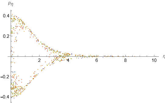
((a)) $E=20$, $\alpha=0.1$, $L=1$. Initial data: $\sigma(0)=2,\ p_{\sigma}(0)=0$ .

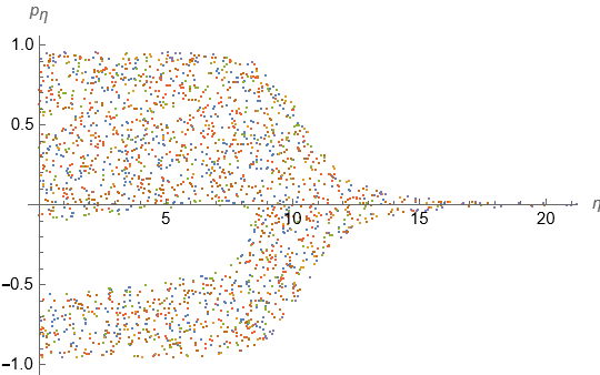
((b)) $E=20$, $\alpha=0.1$, $L=10$. Initial data: $\sigma(0)=2,\ p_{\sigma}(0)=0$ .

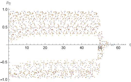
((c)) $E=20$, $\alpha=0.1$, $L=50$. Initial data: $\sigma(0)=2,\ p_{\sigma}(0)=0$ .

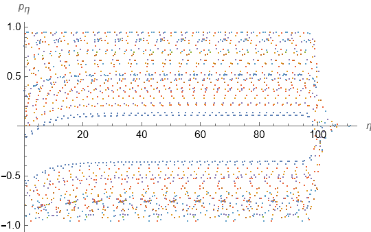
((d)) $E=20$, $\alpha=0.1$, $L=100$. Initial data: $\sigma(0)=2,\ p_{\sigma}(0)=0$ .

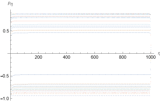
((e)) $E=20$, $\alpha=0.1$, $L=1000$. Initial data: $\sigma(0)=2,\ p_{\sigma}(0)=0$ .

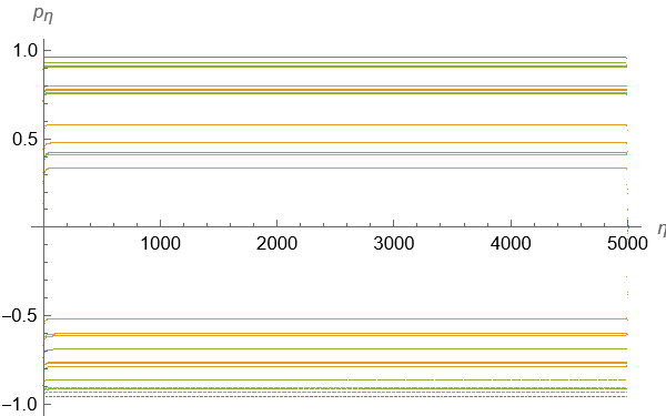
((f)) $E=20$, $\alpha=0.1$, $L=5000$. Initial data: $\sigma(0)=2,\ p_{\sigma}(0)=0$ .

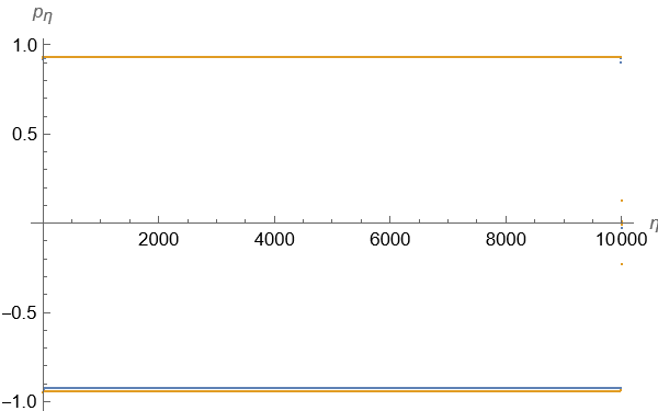
((g)) $E=20$, $\alpha=0.1$, $L=10000$. Initial data: $\sigma(0)=2,\ p_{\sigma}(0)=0$ .

Figure 1: Poincaré sections for the semi-classical string motion in type-IIA background. In the plots we fix the energy of the string as $E=20$ and varying the parameter $L$ from small to very large.

In the following we numerically compute the Lyapunov exponent [9, 10, 11], which is another chaos indicator. For a chaotic system, during the time evolution the system becomes sensitive depending on the choice of initial conditions imposed on the dynamics. The Lyapunov exponent ($\lambda$) provides the deviation between two nearby trajectories in the phase space dynamics due to a variation (small) of the initial conditions .

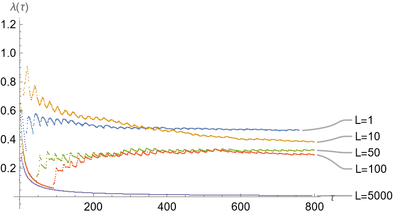
Figure 2: Plots of Lyapunov exponent(s) for the motion of the semi-classical string. We consider different values of parameter $L:\{1,10,50,100,5000\}$ as indicated in the figure while keeping the energy of the string fix at $E=20$ and $\alpha=0.1$.

In Fig.(2) we compute the Lyapunov exponent of our system. We consider the energy of the string as $E=20$ along with the initial separation $\Delta X(0)=10^{-7}$ (cf. (3.30)). In Fig.(2), we observe that upon increasing the values of the parameter $L$, $\lambda$ saturates to zero at sufficient late times indicating corresponding integrable dynamics of the associated phase space.

4 Summary and outlook

In this literature, we study chaotic dynamics of a semi-classical string moving in a class of type-IIA supergravity background that preserves 16 supercharges. The holographic dual of this background is characterised by relevant/irrelevant deformation of the plane wave matrix model depends on the parameter $L$ present in the background [40]. Small $L$ corresponds to relevant deformation and large $L$ corresponds to irrelevant deformation of PWMM.

The main aim of this work was to examine the dynamics of the semi-classical string upon varying the parameter $L$ in a wide range. In the core part of our analysis we consider the Hamiltonian framework and examine Poincaré sections along with the Lyapunov exponents ($\lambda$) for different values of the parameter $L$.

In our analysis we obtain distorted KAM tori as well positive Lyapunov exponents for small values of the parameter $L$ present in the type-IIA supergravity background. This leads us to interpret that the string motion exhibits chaotic behaviour and the system is non-integrable for the small value of the parameter $L$. On the other hand, we observed that string dynamics exhibits an integrable structure for the large value of the parameter $L$ along with vanishing Lyapunov exponent ($\lambda|_{L>>1}\sim 0$). Therefore, our findings show that the parameter $L$ in the dual type-IIA background acts as an interpolation between a non-integrable theory to an integrable theory in dual SCFTs.

From the bulk perspective, the non-integrability of the string dynamics could emerge from the corresponding electrostatic configurations discussed in [42]. In the corresponding electrostatic configuration, addition to the infinite conducting plate at $\eta=0$ we have a set of finite size conducting disks with finite charge $Q_{i}$ at regular intervals along $\eta$-direction ($\eta_{i}$). The presence of these finite size conducting disks along the holographic direction $\eta$ could be an artefact for chaotic string dynamics we observed for small values of the parameter $L$. On the other hand, for the very large values of the parameter $L$, we have only the infinite conducting plate at $\eta=0$ and the finite size conducting disks move to very far distance along $\eta$-direction and that makes string motion smooth and integrable. However, the precise reason of the interpolating string dynamics is lacking in this present literature and requires further investigation. Finally, it will be interesting to identify the precise connection between our findings and the works revealed in [45] and find out the origins of this interpolating behaviour in the dual gauge theory perspective. We hope to report along this line of investigation in the near future.

Acknowledgement

We are indebted to Dibakar Roychowdhury for his insights and discussion on several parts of our work. We would also like to express our gratitude to Carlos Nunez for clarifying several issues along with his key insights on various parts of our work.

Appendix A Warp factors in type-IIA solution

For the potential given in (3.29), the corresponding $F$ and $f_{i}$s in the type-IIA supergravity solution (2.1)-(2.3) take the form

$$F=\frac{\sqrt{F_{N}}}{\sqrt{4\eta-\alpha\bigg{(}\frac{1}{\sqrt{(\eta+L)^{2}+\sigma^{2}}}-\frac{1}{\sqrt{(L-\eta)^{2}+\sigma^{2}}}\bigg{)}-\frac{\alpha L(\eta-L)}{\big{(}(L-\eta)^{2}+\sigma^{2}\big{)}^{3/2}}-\frac{\alpha L(\eta+L)}{\big{(}(\eta+L)^{2}+\sigma^{2}\big{)}^{3/2}}}}\ ,$$ (A.31)

$$F_{N} = \sqrt{\alpha}\Bigg{(}\eta^{2}\bigg{(}\sigma^{2}\bigg{(}\frac{1}{\big{(}(\eta+L)^{2}+\sigma^{2}\big{)}^{3/2}}-\frac{1}{\big{(}(L-\eta)^{2}+\sigma^{2}\big{)}^{3/2}}\bigg{)}-\frac{2}{\sqrt{(L-\eta)^{2}+\sigma^{2}}}+\frac{2}{\sqrt{(\eta+L)^{2}+\sigma^{2}}}\bigg{)}$$

$$+\ \eta L\bigg{(}\sigma^{2}\big{(}\frac{1}{\big{(}(\eta+L)^{2}+\sigma^{2}\big{)}^{3/2}}+\frac{1}{\big{(}(L-\eta)^{2}+\sigma^{2}\big{)}^{3/2}}\big{)}+2\big{(}\frac{1}{\sqrt{(\eta+L)^{2}+\sigma^{2}}}+\frac{1}{\sqrt{(L-\eta)^{2}+\sigma^{2}}}\big{)}\bigg{)}$$

$$+\ \sigma^{4}\bigg{(}\frac{1}{\big{(}(\eta+L)^{2}+\sigma^{2}\big{)}^{3/2}}-\frac{1}{\big{(}(L-\eta)^{2}+\sigma^{2}\big{)}^{3/2}}\bigg{)}\Bigg{)}\ ,$$

$$f_{1}=-\frac{f_{1N}}{f_{1D}}\ ,$$

$$f_{1N} = 4\sigma\bigg{(}\alpha\sigma\bigg{(}\frac{\eta^{2}+2L^{2}-2\eta L+\sigma^{2}}{\big{(}(L-\eta)^{2}+\sigma^{2}\big{)}^{3/2}}+\frac{\sigma^{2}}{\big{(}(\eta+L)^{2}+\sigma^{2}\big{)}^{3/2}}-\frac{2}{\sqrt{(\eta+L)^{2}+\sigma^{2}}}\bigg{)}+\frac{\alpha\eta^{2}\sigma}{\big{(}(\eta+L)^{2}+\sigma^{2}\big{)}^{3/2}}$$

$$+\ \eta\sigma\bigg{(}\alpha L\big{(}\frac{1}{\big{(}(\eta+L)^{2}+\sigma^{2}\big{)}^{3/2}}-\frac{1}{\big{(}(L-\eta)^{2}+\sigma^{2}\big{)}^{3/2}}\big{)}+4\bigg{)}\bigg{)}\ ,$$

$$f_{1D} = \alpha\bigg{(}\eta^{2}\bigg{(}\sigma^{2}\big{(}\frac{1}{\big{(}(\eta+L)^{2}+\sigma^{2}\big{)}^{3/2}}-\frac{1}{\big{(}(L-\eta)^{2}+\sigma^{2}\big{)}^{3/2}}\big{)}-\frac{2}{\sqrt{(L-\eta)^{2}+\sigma^{2}}}+\frac{2}{\sqrt{(\eta+L)^{2}+\sigma^{2}}}\bigg{)}$$

$$+\ \eta L\bigg{(}\sigma^{2}\big{(}\frac{1}{\big{(}(\eta+L)^{2}+\sigma^{2}\big{)}^{3/2}}+\frac{1}{\big{(}(L-\eta)^{2}+\sigma^{2}\big{)}^{3/2}}\big{)}+2\big{(}\frac{1}{\sqrt{(\eta+L)^{2}+\sigma^{2}}}+\frac{1}{\sqrt{(L-\eta)^{2}+\sigma^{2}}}\big{)}\bigg{)}$$

$$+\ \sigma^{4}\big{(}\frac{1}{\big{(}(\eta+L)^{2}+\sigma^{2}\big{)}^{3/2}}-\frac{1}{\big{(}(L-\eta)^{2}+\sigma^{2}\big{)}^{3/2}}\big{)}\bigg{)}\ ,$$

$$f_{2}=-\frac{2\left(-4\eta+\alpha\left(\frac{1}{\sqrt{(\eta+L)^{2}+\sigma^{2}}}-\frac{1}{\sqrt{(L-\eta)^{2}+\sigma^{2}}}\right)+\frac{\alpha L(\eta-L)}{\left((L-\eta)^{2}+\sigma^{2}\right)^{3/2}}+\frac{\alpha L(\eta+L)}{\left((\eta+L)^{2}+\sigma^{2}\right)^{3/2}}\right)}{-\frac{\alpha L^{2}}{\sqrt{(L-\eta)^{2}+\sigma^{2}}}-\frac{\alpha\left(\eta^{2}+2\eta L+\sigma^{2}\right)}{\sqrt{(\eta+L)^{2}+\sigma^{2}}}+\eta\left(\alpha L\left(\frac{1}{\sqrt{(\eta+L)^{2}+\sigma^{2}}}+\frac{1}{\sqrt{(L-\eta)^{2}+\sigma^{2}}}\right)+2\sigma^{2}\right)+\alpha\sqrt{(L-\eta)^{2}+\sigma^{2}}}\ ,$$

$$f_{3}=4\ ,$$

$$f_{4}=\frac{f_{4N}}{f_{4D}}\ ,$$

$$f_{4N} = 2\bigg{(}-4\eta+\alpha\big{(}\frac{1}{\sqrt{(\eta+L)^{2}+\sigma^{2}}}-\frac{1}{\sqrt{(L-\eta)^{2}+\sigma^{2}}}\big{)}+\frac{\alpha L(\eta-L)}{\big{(}(L-\eta)^{2}+\sigma^{2}\big{)}^{3/2}}+\frac{\alpha L(\eta+L)}{\big{(}(\eta+L)^{2}+\sigma^{2}\big{)}^{3/2}}\bigg{)}$$

$$\bigg{(}-\frac{\alpha L^{2}}{\sqrt{(L-\eta)^{2}+\sigma^{2}}}-\frac{\alpha\big{(}\eta^{2}+2\eta L+\sigma^{2}\big{)}}{\sqrt{(\eta+L)^{2}+\sigma^{2}}}+\eta\bigg{(}\alpha L\bigg{(}\frac{1}{\sqrt{(\eta+L)^{2}+\sigma^{2}}}+\frac{1}{\sqrt{(L-\eta)^{2}+\sigma^{2}}}\bigg{)}+2\sigma^{2}\bigg{)}$$

$$+\ \alpha\sqrt{(L-\eta)^{2}+\sigma^{2}}\bigg{)}\ ,$$

$$f_{4D} = \bigg{(}-4\eta+\alpha\big{(}\frac{1}{\sqrt{(\eta+L)^{2}+\sigma^{2}}}-\frac{1}{\sqrt{(L-\eta)^{2}+\sigma^{2}}}\big{)}+\frac{\alpha L(\eta-L)}{\big{(}(L-\eta)^{2}+\sigma^{2}\big{)}^{3/2}}+\frac{\alpha L(\eta+L)}{\big{(}(\eta+L)^{2}+\sigma^{2}\big{)}^{3/2}}\bigg{)}$$

$$\bigg{(}\sigma\bigg{(}\alpha\sigma\bigg{(}\frac{\eta^{2}+2L^{2}-2\eta L+\sigma^{2}}{\big{(}(L-\eta)^{2}+\sigma^{2}\big{)}^{3/2}}+\frac{\sigma^{2}}{\big{(}(\eta+L)^{2}+\sigma^{2}\big{)}^{3/2}}-\frac{2}{\sqrt{(\eta+L)^{2}+\sigma^{2}}}\bigg{)}+\frac{\alpha\eta^{2}\sigma}{\big{(}(\eta+L)^{2}+\sigma^{2}\big{)}^{3/2}}$$

$$+\ \eta\sigma\big{(}\alpha L\bigg{(}\frac{1}{\big{(}(\eta+L)^{2}+\sigma^{2}\big{)}^{3/2}}-\frac{1}{\big{(}(L-\eta)^{2}+\sigma^{2}\big{)}^{3/2}}\bigg{)}+4\big{)}\bigg{)}+\frac{2\alpha L^{2}}{\sqrt{(L-\eta)^{2}+\sigma^{2}}}$$

$$+\ \frac{2\alpha\big{(}\eta^{2}+2\eta L+\sigma^{2}\big{)}}{\sqrt{(\eta+L)^{2}+\sigma^{2}}}-2\eta\big{(}\alpha L\bigg{(}\frac{1}{\sqrt{(\eta+L)^{2}+\sigma^{2}}}+\frac{1}{\sqrt{(L-\eta)^{2}+\sigma^{2}}}\bigg{)}+2\sigma^{2}\big{)}$$

$$-\ 2\alpha\sqrt{(L-\eta)^{2}+\sigma^{2}}\bigg{)}-\bigg{(}\sigma^{2}\bigg{(}\alpha L\bigg{(}\frac{1}{\big{(}(\eta+L)^{2}+\sigma^{2}\big{)}^{3/2}}+\frac{1}{\big{(}(L-\eta)^{2}+\sigma^{2}\big{)}^{3/2}}\bigg{)}$$

$$+\ \frac{\alpha}{\sqrt{(L-\eta)^{2}+\sigma^{2}}\big{(}-\eta+\sqrt{(L-\eta)^{2}+\sigma^{2}}+L\big{)}}+\frac{\alpha}{\sqrt{(\eta+L)^{2}+\sigma^{2}}\big{(}\eta+\sqrt{(\eta+L)^{2}+\sigma^{2}}+L\big{)}}$$

$$+\ 2\bigg{)}-2\alpha\bigg{)}^{2}\ ,$$

$$f_{5}=2\bigg{(}\eta+\frac{f_{5N}}{f_{5D}}\bigg{)}\ ,$$

$$f_{5N} = \bigg{(}-\frac{\alpha L^{2}}{\sqrt{(L-\eta)^{2}+\sigma^{2}}}-\frac{\alpha\big{(}\eta^{2}+2\eta L+\sigma^{2}\big{)}}{\sqrt{(\eta+L)^{2}+\sigma^{2}}}+\eta\bigg{(}\alpha L\bigg{(}\frac{1}{\sqrt{(\eta+L)^{2}+\sigma^{2}}}+\frac{1}{\sqrt{(L-\eta)^{2}+\sigma^{2}}}\bigg{)}+2\sigma^{2}\bigg{)}$$

$$+\ \alpha\sqrt{(L-\eta)^{2}+\sigma^{2}}\bigg{)}\times\bigg{(}\sigma^{2}\big{(}\alpha L\bigg{(}\frac{1}{\big{(}(\eta+L)^{2}+\sigma^{2}\big{)}^{3/2}}+\frac{1}{\big{(}(L-\eta)^{2}+\sigma^{2}\big{)}^{3/2}}\bigg{)}$$

$$+\ \frac{\alpha}{\sqrt{(L-\eta)^{2}+\sigma^{2}}\big{(}-\eta+\sqrt{(L-\eta)^{2}+\sigma^{2}}+L\big{)}}+\frac{\alpha}{\sqrt{(\eta+L)^{2}+\sigma^{2}}\bigg{(}\eta+\sqrt{(\eta+L)^{2}+\sigma^{2}}+L\bigg{)}}$$

$$+\ 2\big{)}-2\alpha\bigg{)}\ ,$$

$$f_{5D} = \bigg{(}-4\eta+\alpha\big{(}\frac{1}{\sqrt{(\eta+L)^{2}+\sigma^{2}}}-\frac{1}{\sqrt{(L-\eta)^{2}+\sigma^{2}}}\big{)}+\frac{\alpha L(\eta-L)}{\big{(}(L-\eta)^{2}+\sigma^{2}\big{)}^{3/2}}+\frac{\alpha L(\eta+L)}{\big{(}(\eta+L)^{2}+\sigma^{2}\big{)}^{3/2}}\bigg{)}$$

$$\bigg{(}\sigma\bigg{(}\alpha\sigma\bigg{(}\frac{\eta^{2}+2L^{2}-2\eta L+\sigma^{2}}{\big{(}(L-\eta)^{2}+\sigma^{2}\big{)}^{3/2}}+\frac{\sigma^{2}}{\big{(}(\eta+L)^{2}+\sigma^{2}\big{)}^{3/2}}-\frac{2}{\sqrt{(\eta+L)^{2}+\sigma^{2}}}\bigg{)}+\frac{\alpha\eta^{2}\sigma}{\big{(}(\eta+L)^{2}+\sigma^{2}\big{)}^{3/2}}$$

$$+\ \eta\sigma\bigg{(}\alpha L\bigg{(}\frac{1}{\big{(}(\eta+L)^{2}+\sigma^{2}\big{)}^{3/2}}-\frac{1}{\big{(}(L-\eta)^{2}+\sigma^{2}\big{)}^{3/2}}\bigg{)}+4\bigg{)}\bigg{)}+\frac{2\alpha L^{2}}{\sqrt{(L-\eta)^{2}+\sigma^{2}}}$$

$$+\ \frac{2\alpha\big{(}\eta^{2}+2\eta L+\sigma^{2}\big{)}}{\sqrt{(\eta+L)^{2}+\sigma^{2}}}-2\eta\bigg{(}\alpha L\bigg{(}\frac{1}{\sqrt{(\eta+L)^{2}+\sigma^{2}}}+\frac{1}{\sqrt{(L-\eta)^{2}+\sigma^{2}}}\bigg{)}+2\sigma^{2}\bigg{)}$$

$$-\ 2\alpha\sqrt{(L-\eta)^{2}+\sigma^{2}}\bigg{)}-\bigg{(}\sigma^{2}\big{(}\alpha L\bigg{(}\frac{1}{\big{(}(\eta+L)^{2}+\sigma^{2}\big{)}^{3/2}}+\frac{1}{\big{(}(L-\eta)^{2}+\sigma^{2}\big{)}^{3/2}}\bigg{)}$$

$$+\ \frac{\alpha}{\sqrt{(L-\eta)^{2}+\sigma^{2}}\bigg{(}-\eta+\sqrt{(L-\eta)^{2}+\sigma^{2}}+L\bigg{)}}+\frac{\alpha}{\sqrt{(\eta+L)^{2}+\sigma^{2}}\bigg{(}\eta+\sqrt{(\eta+L)^{2}+\sigma^{2}}+L\bigg{)}}$$

$$+\ 2\big{)}-2\alpha\bigg{)}^{2}\ .$$

Appendix B Poincaré section to string motion for general windings

In this appendix, we study phase space plots corresponding to the string configurations with general values of the winding numbers $\{k_{1},k_{2}\}>1$. For examples, in Figs.(3(a))-(3(b)) we consider the winding numbers $\{k_{1}=k_{2}=2\}$ and the parameter $L=\{1,10\}$.

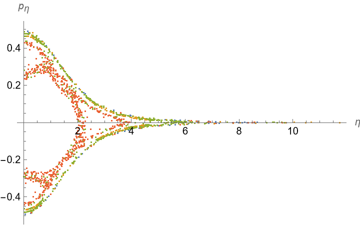
((a)) $E=35,\ L=1,\ k_{1}=2=k_{2},\ \alpha=0.1$.

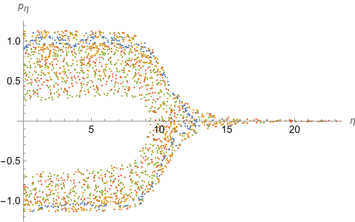
((b)) $E=35,\ L=10,\ k_{1}=2=k_{2},\ \alpha=0.1$.

Figure 3: Poincaré sections for winding $k_{1}=k_{2}=2$ with $L:\{1,10\}$ . Here we set the energy $E=35$ and $\alpha=0.1$ in both cases.

It is very straightforward to see from Figs.(3(a))-(3(b)) that irrespective of the values of the winding numbers $k_{i}(i=1,2)$ the Poincaré sections do not change qualitatively and exhibits chaotic motion in nature.

Appendix C Poincaré section to string motion in the non-Abelian T-dual background

In the following we provide phase space plots corresponding to the string configurations moving in non-Abelian T-dual of AdS background. The corresponding potential function $V(\sigma,\eta)$ is given by

$$V(\sigma,\eta)=\eta\Bigg{[}\frac{\sigma^{2}}{2}-\ln\sigma-\frac{\eta^{2}}{3}\Bigg{]}\ .$$ (C.32)

In the plots (Fig. (4(a))-(4(b))) we choose the winding numbers $\{k_{1}=k_{2}=1\}$ and $\{k_{1}=k_{2}=5\}$. Here the phase space dynamics exhibits integrable structure.

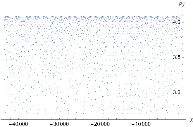
((a)) $k_{1}=k_{2}=1$ .

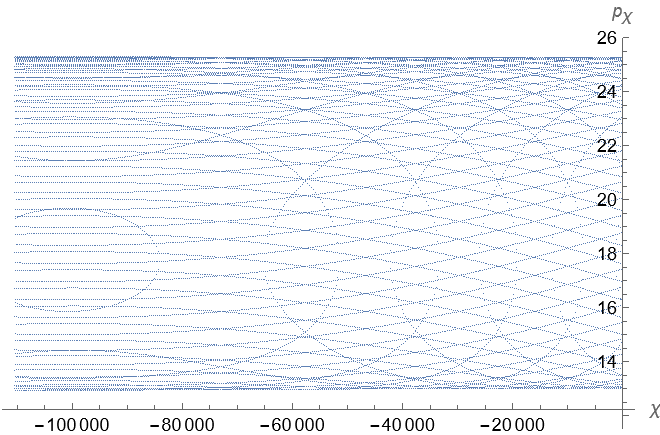
((b)) $k_{1}=k_{2}=5$ .

Figure 4: Poincaré sections for non-Abelian T-dual solution. Here we set the energy $E=0.5$  , $\eta=1\ ,\ p_{\eta}=0$ in both cases.

Appendix D Brief review of type-IIA supergravity

For massive type-IIA supergravity, the field strengths are given by

$$H_{3}=dB_{2}\ ;\ F_{2}=dC_{1}+F_{0}B_{2}\ ;\ F_{4}=dC_{3}-H_{3}\wedge C_{1}+\frac{F_{0}}{2}B_{2}\wedge B_{2}\ .$$ (D.33)

The field strenghts are invariant under the gauge transformations

$$\delta B_{2}=d\Lambda_{1}\ ;\ \delta C_{1}=-F_{0}\Lambda_{1}\ ;\ \delta C_{3}=-F_{0}\Lambda_{1}\wedge B_{2}\ ,$$ (D.34)

where $\Lambda$ is a one-form. The Bianchi identities become

$$dH_{3}=0\ ;\ dF_{2}=F_{0}H_{3}\ ;\ dF_{4}=H_{3}\wedge F_{2}\ .$$ (D.35)

The action of the massive type-IIA supergravity is

$$S=\frac{1}{2k^{2}}\int_{M_{10}}\sqrt{-g} \Bigg{[} e^{-2\Phi}\Big{(}R+4(\partial\Phi)^{2}-\frac{H_{3}^{2}}{12}\Big{)}-\frac{1}{2}\Big{(}F_{0}^{2}+\frac{F_{2}^{2}}{2}+\frac{F_{4}^{2}}{4!}\Big{)}\Bigg{]}$$ (D.37)

$$-\frac{1}{2}\Bigg{[}dC_{3}\wedge dC_{3}\wedge B_{2}+\frac{F_{0}}{3}dC_{3}\wedge B^{3}+\frac{F_{0}^{2}}{20}B_{2}^{5}\Bigg{]}\ .$$

Einstein’s equations are

$$R_{\mu\nu}+2D_{\mu}D_{\nu}\Phi=\frac{1}{4}H_{\mu\nu}^{2}+e^{2\Phi}\Bigg{[}\frac{1}{2}(F_{2}^{2})_{\mu\nu}+\frac{1}{12}(F_{4}^{2})_{\mu\nu}-\frac{1}{4}g_{\mu\nu}\Big{(}F_{0}^{2}+\frac{1}{2}F_{2}^{2}+\frac{1}{4!}F_{4}^{2}\Big{)}\Bigg{]}\ .$$ (D.38)

The equation coming from varying the dilaton is

$$R+4D^{2}\Phi-4(\partial\Phi)^{2}-\frac{1}{12}H_{3}^{2}=0\ .$$ (D.39)

The equation of motion for the gauge fields in type-IIA case are given by

$$d\Big{(}e^{-2\Phi}\star H_{3}\Big{)}-F_{2}\wedge\star F_{4}-\frac{1}{2}F_{4}\wedge F_{4} = F_{0}\star F_{2}\ ,$$ (D.40)

$$d\star F_{2}+H_{3}\wedge\star F_{4} = 0\ ,$$ (D.41)

$$d\star F_{4}+H_{3}\wedge F_{4} = 0\ .$$ (D.42)

References

• [1] J. M. Maldacena, “The Large N limit of superconformal field theories and supergravity,” Adv. Theor. Math. Phys. 2, 231-252 (1998) doi:10.4310/ATMP.1998.v2.n2.a1 [arXiv:hep-th/9711200 [hep-th]].
• [2] E. Witten, “Anti-de Sitter space and holography,” Adv. Theor. Math. Phys. 2, 253-291 (1998) doi:10.4310/ATMP.1998.v2.n2.a2 [arXiv:hep-th/9802150 [hep-th]].
• [3] K. Sfetsos, “Integrable interpolations: From exact CFTs to non-Abelian T-duals,” Nucl. Phys. B 880, 225-246 (2014) doi:10.1016/j.nuclphysb.2014.01.004 [arXiv:1312.4560 [hep-th]].
• [4] T. J. Hollowood, J. L. Miramontes and D. M. Schmidtt, “An Integrable Deformation of the $AdS_{5}\times S^{5}$ Superstring,” J. Phys. A 47, no.49, 495402 (2014) doi:10.1088/1751-8113/47/49/495402 [arXiv:1409.1538 [hep-th]].
• [5] F. Delduc, M. Magro and B. Vicedo, “An integrable deformation of the $AdS_{5}\times S^{5}$ superstring action,” Phys. Rev. Lett. 112, no.5, 051601 (2014) doi:10.1103/PhysRevLett.112.051601 [arXiv:1309.5850 [hep-th]].
• [6] J. Pal, H. Rathi, A. Lala and D. Roychowdhury, “Non-chaotic dynamics for Yang-Baxter deformed $AdS_{4}\times CP^{3}$ superstrings,” [arXiv:2208.09599 [hep-th]].
• [7] D. Roychowdhury, “Analytic integrability for holographic duals with $J\overline{T}$ deformations,” JHEP 09, 053 (2020) doi:10.1007/JHEP09(2020)053 [arXiv:2005.04457 [hep-th]].
• [8] K. Filippas, C. Núñez and J. Van Gorsel, “Integrability and holographic aspects of six-dimensional $\mathcal{N}=\left(1,\ 0\right)$ superconformal field theories,” JHEP 06, 069 (2019) doi:10.1007/JHEP06(2019)069 [arXiv:1901.08598 [hep-th]].
• [9] L. A. Pando Zayas and C. A. Terrero-Escalante, “Chaos in the Gauge / Gravity Correspondence,” JHEP 09, 094 (2010) doi:10.1007/JHEP09(2010)094 [arXiv:1007.0277 [hep-th]].
• [10] P. Basu, D. Das and A. Ghosh, “Integrability Lost,” Phys. Lett. B 699, 388-393 (2011) doi:10.1016/j.physletb.2011.04.027 [arXiv:1103.4101 [hep-th]].
• [11] P. Basu and L. A. Pando Zayas, “Chaos rules out integrability of strings on AdS${}_{5}\times T^{1,1}$,” Phys. Lett. B 700, 243-248 (2011) doi:10.1016/j.physletb.2011.04.063 [arXiv:1103.4107 [hep-th]].
• [12] P. Basu and L. A. Pando Zayas, “Analytic Non-integrability in String Theory,” Phys. Rev. D 84, 046006 (2011) doi:10.1103/PhysRevD.84.046006 [arXiv:1105.2540 [hep-th]].
• [13] P. Basu, D. Das, A. Ghosh and L. A. Pando Zayas, “Chaos around Holographic Regge Trajectories,” JHEP 05, 077 (2012) doi:10.1007/JHEP05(2012)077 [arXiv:1201.5634 [hep-th]].
• [14] L. A. Pando Zayas and D. Reichmann, “A String Theory Explanation for Quantum Chaos in the Hadronic Spectrum,” JHEP 04, 083 (2013) doi:10.1007/JHEP04(2013)083 [arXiv:1209.5902 [hep-th]].
• [15] P. Basu and A. Ghosh, “Confining Backgrounds and Quantum Chaos in Holography,” Phys. Lett. B 729, 50-55 (2014) doi:10.1016/j.physletb.2013.12.052 [arXiv:1304.6348 [hep-th]].
• [16] P. Basu, P. Chaturvedi and P. Samantray, “Chaotic dynamics of strings in charged black hole backgrounds,” Phys. Rev. D 95, no.6, 066014 (2017) doi:10.1103/PhysRevD.95.066014 [arXiv:1607.04466 [hep-th]].
• [17] K. L. Panigrahi and M. Samal, “Chaos in classical string dynamics in $\hat{\gamma}$ deformed $AdS_{5}\times T^{1,1}$,” Phys. Lett. B 761, 475-481 (2016) doi:10.1016/j.physletb.2016.08.021 [arXiv:1605.05638 [hep-th]].
• [18] D. Giataganas, L. A. Pando Zayas and K. Zoubos, “On Marginal Deformations and Non-Integrability,” JHEP 01, 129 (2014) doi:10.1007/JHEP01(2014)129 [arXiv:1311.3241 [hep-th]].
• [19] T. Ishii, S. Kushiro and K. Yoshida, “Chaotic string dynamics in deformed T1,1,” JHEP 05, 158 (2021) doi:10.1007/JHEP05(2021)158 [arXiv:2103.12416 [hep-th]].
• [20] D. Roychowdhury, “Analytic integrability for strings on $\eta$ and $\lambda$ deformed backgrounds,” JHEP 10, 056 (2017) doi:10.1007/JHEP10(2017)056 [arXiv:1707.07172 [hep-th]].
• [21] C. Núñez, J. M. Penín, D. Roychowdhury and J. Van Gorsel, “‘The non-Integrability of Strings in Massive Type IIA and their Holographic duals,” JHEP 06, 078 (2018) doi:10.1007/JHEP06(2018)078 [arXiv:1802.04269 [hep-th]].
• [22] C. Nunez, D. Roychowdhury and D. C. Thompson, “Integrability and non-integrability in $\mathcal{N}=2$ SCFTs and their holographic backgrounds,” JHEP 07, 044 (2018) doi:10.1007/JHEP07(2018)044 [arXiv:1804.08621 [hep-th]].
• [23] A. Banerjee and A. Bhattacharyya, “Probing analytical and numerical integrability: the curious case of (AdS${}_{5}\times S^{5}$)η,” JHEP 11, 124 (2018) doi:10.1007/JHEP11(2018)124 [arXiv:1806.10924 [hep-th]].
• [24] K. S. Rigatos, “Nonintegrability of $L^{a,b,c}$ quiver gauge theories,” Phys. Rev. D 102, no.10, 106022 (2020) doi:10.1103/PhysRevD.102.106022 [arXiv:2009.11878 [hep-th]].
• [25] D. Giataganas and K. Zoubos, “Non-integrability and Chaos with Unquenched Flavor,” JHEP 10, 042 (2017) doi:10.1007/JHEP10(2017)042 [arXiv:1707.04033 [hep-th]].
• [26] K. Filippas, “Non-integrability on AdS3 supergravity backgrounds,” JHEP 02, 027 (2020) doi:10.1007/JHEP02(2020)027 [arXiv:1910.12981 [hep-th]].
• [27] K. Filippas, “Nonintegrability of the $\Omega$ deformation,” Phys. Rev. D 101, no.4, 046025 (2020) doi:10.1103/PhysRevD.101.046025 [arXiv:1912.03791 [hep-th]].
• [28] I. Bena, J. Polchinski and R. Roiban, “Hidden symmetries of the $AdS_{5}\times S^{5}$ superstring,” Phys. Rev. D 69, 046002 (2004) doi:10.1103/PhysRevD.69.046002 [arXiv:hep-th/0305116 [hep-th]].
• [29] G. Arutyunov and S. Frolov, “Superstrings on $AdS_{4}\times CP^{3}$ as a Coset Sigma-model,” JHEP 09, 129 (2008) doi:10.1088/1126-6708/2008/09/129 [arXiv:0806.4940 [hep-th]].
• [30] B. Stefanski, jr, “Green-Schwarz action for Type IIA strings on $AdS_{4}\times CP^{3}$,” Nucl. Phys. B 808, 80-87 (2009) doi:10.1016/j.nuclphysb.2008.09.015 [arXiv:0806.4948 [hep-th]].
• [31] D. Sorokin and L. Wulff, “‘Evidence for the classical integrability of the complete $AdS_{4}\times CP^{3}$ superstring,” JHEP 11, 143 (2010) doi:10.1007/JHEP11(2010)143 [arXiv:1009.3498 [hep-th]].
• [32] K. Zarembo, “Strings on Semisymmetric Superspaces,” JHEP 05, 002 (2010) doi:10.1007/JHEP05(2010)002 [arXiv:1003.0465 [hep-th]].
• [33] S. Frolov, “Lax pair for strings in Lunin-Maldacena background,” JHEP 05, 069 (2005) doi:10.1088/1126-6708/2005/05/069 [arXiv:hep-th/0503201 [hep-th]].
• [34] J. J.  Kovacic, “An algorithm for solving second order linear homogeneous differential equations,” J. Symb. Comput. 2 (1986) 3.
• [35] B.  D.  Saunders, “An implementation of Kovacic’s algorithm for solving second order linear homogeneous differential equations,” The Proceedings of the 4th ACM Symposium on Symbolic and Algebraic Computation, SYMSAC’81, August 5–7, Snowbird, USA, 1981.
• [36] J. J.  Kovacic, “Picard-Vessiot Theory, Algebraic Groups and Group Schemes,” Department of Mathematics, the City College of the City University of New York, 2005.
• [37] C. Núñez, D. Roychowdhury, S. Speziali and S. Zacarías, “Holographic aspects of four dimensional ${\cal N}=2$ SCFTs and their marginal deformations,” Nucl. Phys. B 943, 114617 (2019) doi:10.1016/j.nuclphysb.2019.114617 [arXiv:1901.02888 [hep-th]].
• [38] J. Pal, S. Roychowdhury, A. Lala and D. Roychowdhury, “Integrability and non-integrability for marginal deformations of 4d $\mathcal{N}=2$ SCFTs,” [arXiv:2307.12079 [hep-th]].
• [39] D. E. Berenstein, J. M. Maldacena and H. S. Nastase, “Strings in flat space and pp waves from $\mathcal{N}=4$ superYang-Mills,” JHEP 04, 013 (2002) doi:10.1088/1126-6708/2002/04/013 [arXiv:hep-th/0202021 [hep-th]].
• [40] Y. Lozano, C. Nunez and S. Zacarias, “BMN Vacua, Superstars and Non-Abelian T-duality,” JHEP 09, 008 (2017) doi:10.1007/JHEP09(2017)008 [arXiv:1703.00417 [hep-th]].
• [41] H. Lin, “The Supergravity dual of the BMN matrix model,” JHEP 12, 001 (2004) doi:10.1088/1126-6708/2004/12/001 [arXiv:hep-th/0407250 [hep-th]].
• [42] H. Lin and J. M. Maldacena, “Fivebranes from gauge theory,” Phys. Rev. D 74, 084014 (2006) doi:10.1103/PhysRevD.74.084014 [arXiv:hep-th/0509235 [hep-th]].
• [43] H. Lin, O. Lunin and J. M. Maldacena, “Bubbling AdS space and 1/2 BPS geometries,” JHEP 10, 025 (2004) doi:10.1088/1126-6708/2004/10/025 [arXiv:hep-th/0409174 [hep-th]].
• [44] D. Roychowdhury, “Matrix model correlators from non-Abelian T-dual of $AdS_{5}\times S^{5}$,” [arXiv:2310.10210 [hep-th]].
• [45] Y. Asano, D. Kawai and K. Yoshida, “Chaos in the BMN matrix model,” JHEP 06, 191 (2015) doi:10.1007/JHEP06(2015)191 [arXiv:1503.04594 [hep-th]].