Graph Sphere: From Nodes to Supernodes in Graphical Models

Abstract

High-dimensional data analysis typically focuses on low-dimensional structure, often to aid interpretation and computational efficiency. Graphical models provide a powerful methodology for learning the conditional independence structure in multivariate data by representing variables as nodes and dependencies as edges. Inference is often focused on individual edges in the latent graph. Nonetheless, there is increasing interest in determining more complex structures, such as communities of nodes, for multiple reasons, including more effective information retrieval and better interpretability. In this work, we propose a multilayer graphical model where we first cluster nodes and then, at the second layer, investigate the relationships among groups of nodes. Specifically, nodes are partitioned into supernodes with a data-coherent size-biased tessellation prior which combines ideas from Bayesian nonparametrics and Voronoi tessellations. This construct allows accounting also for dependence of nodes within supernodes. At the second layer, dependence structure among supernodes is modelled through a Gaussian graphical model, where the focus of inference is on superedges. We provide theoretical justification for our modelling choices. We design tailored Markov chain Monte Carlo schemes, which also enable parallel computations. We demonstrate the effectiveness of our approach for large-scale structure learning in simulations and a transcriptomics application.

Keywords: Bayesian statistics, cutting feedback, gene co-expression network analysis, multilayer Gaussian graphical models, random Voronoi tessellations.

1 Introduction

In applications with many variables, interest often lies in identifying large-scale structure. For instance, groups of variables might carry meaning such as when dividing genes into co-expression modules (Saelens et al.,, 2018) or in item response theory (Bock & Gibbons,, 2021), where latent traits are associated with sets of questionnaire items. Furthermore, the relationship between variables and, more importantly at a larger scale, among the groups they belong to can elucidate pre-eminent patterns in data. We therefore introduce a multilayer graphical model which clusters variables, and learns structure both within and among clusters.

Graphical models describe the dependencies in multivariate data by associating nodes of a graph with variables and the edges between them with conditional dependencies (Lauritzen,, 1996). For graphs, inferential focus has shifted from single edges to large-scale structure (Fienberg,, 2012; Barabási,, 2016). Such advances are driven by the increasing amount of available data and the complex patterns discovered in them. Specifically, data exhibit mesoscopic patterns, such as metabolic or signalling pathways, that cannot be explained by models that use single edges as the main building block (Iñiguez et al.,, 2020). This new direction represents a change in perspective from a reductionist viewpoint, with a shift from graph structures described through pairwise interaction between nodes, towards use of large-scale structures (Barabási,, 2012) for tackling the complexity present in empirical data.

Detecting substructures allows gaining better insight into the intricate patterns and dependencies within these systems. This is crucial in various fields such as bioinformatics (e.g. identifying functional motifs in biological networks) and social network analysis (e.g. detecting common structural patterns in social networks: for instance, subgraphs in criminal networks can reveal hidden patterns of criminal behaviour). A large-scale feature that has received specific attention is that of modularity or grouping of nodes (Newman,, 2012) which for instance appears in genetics (Saelens et al.,, 2018), metabolomics (Ravasz et al.,, 2002), brain connectomes (Sporns & Betzel,, 2016) and protein-protein interactions (Yook et al.,, 2004), shifting the focus from single edges to graph substructures.

In the literature, there exist proposals on how to extend graphical models to learn groupings of nodes (e.g. Peixoto,, 2019; van den Boom et al., 2022b, ). While these methods focus on larger structure, they are still based on inference of edges between individual variables, with the number of possible graphs growing superexponentially with the number of nodes. Also, in the context of Gaussian graphical models (GGMs, Dempster,, 1972), detection of individual edges reduces to testing for partial correlations which is especially difficult (Knudson & Lindsey,, 2014). The effects on inference are exemplified by the GGM simulation study in online Appendix LABEL:ap:ROC_simul where increasingly many observations are required for reasonable recovery of edges with a larger number of nodes.

To overcome these challenges, we devise a multilayer construction which goes beyond edges between individual variables. Similarly to previous works, we cluster nodes into groups. However, we then follow a different strategy from the existing literature. Specifically, we treat the groups of nodes as supernodes (which represent macrostructure) and connect them using superedges. Such superedges act at a higher level, connecting supernodes in what we call the supergraph. Within each supernode, the conditional independence structure is captured by a traditional GGM, with edges linking individual nodes. Note that edges between individual variables only appear within supernodes, but not across. We call this multilayer construction a graph sphere because it is reminiscent of the organisation of stars into constellations in the celestial sphere.

To give an intuition of our modelling strategy, Figure 1 contains an example of a graph sphere inferred from gene expression data (see Section 4 for details), alongside a modular structure found by Zhang, (2018) for the same data. We are able to detect a rich structure among the genes which is notably more granular than the one found in Zhang, (2018). Figure 1 shows the partition of nodes into modules (supernodes) as well as the dependency structure among them (superedges), aiding interpretation and unveiling underlying biological mechanisms. This result needs to be contrasted with the single-layer analysis in Zhang, (2018) and the analysis from a standard GGM model shown in Figure LABEL:fig:gene_glasso in Supplementary Material. We note that further inspection reveals that the finer granularity in the identified modules is supported by the literature.

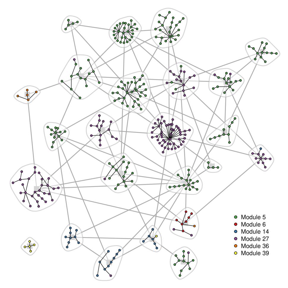
Figure 1: Gene expression data: graph sphere estimated from nested MCMC. The circles represent nodes (i.e. genes) which are connected by the within-supernode graphs (trees) in black. Trees are encircled in grey to mark the supernodes. Grey lines identify superedges between supernodes. The nodes are coloured according to the modules in Zhang, (2018).

Within the Bayesian framework, we construct a data-coherent prior on the clustering of nodes into supernodes which has two main components: (i) a random tessellation (Denison et al., 2002a, ; Denison et al., 2002b, ) to enforce that highly correlated variables are grouped together; (ii) a size-biased term to inform the size of the grouping (Betancourt et al.,, 2022). Thus, the prior is highly informative and driven by structure in the data.

Informative priors are common in high-dimensional problems, like the horseshoe prior for sparse linear regression (Bhadra et al.,, 2019). Such priors often do not reflect prior beliefs, but facilitate posterior inference, for instance asymptotically and relative to uninformative priors. Although priors should represent subjective beliefs, there is in principle no reason against the use of data-dependent or data-coherent priors (Martin & Walker,, 2019). Furthermore, they are sometimes preferred as they lead to posterior distributions satisfying desirable frequentist properties. For instance, the variable selection priors in Martin et al., (2017) and Liu et al., (2021) depend on data through centring at a maximum likelihood estimate. We similarly use data information in our prior to obtain inference in line with our goals of dimensionality reduction and large-scale dependency discovery.

As the likelihood for the supergraph, we specify a GGM that links supernodes, specifically on the first principal components obtained from the variables within each supernode. We theoretically justify our modelling strategy. The resulting likelihood does not correspond to a data generating process. Such likelihoods are gaining in popularity as it is increasingly difficult to specify a model that fully captures data complexity in high-dimensional problems. In this context, our model has connections with different approaches: (i) indirect likelihood, which derives from an (auxiliary) model on a transformation of the data (Drovandi et al.,, 2015); (ii) restricted likelihood, which is defined through an insufficient statistic of the data (see Lewis et al.,, 2021, for an overview); (iii) the likelihood in a Gibbs posterior, which is based on a loss function instead of a distribution on the data (e.g. Jiang & Tanner,, 2008). These likelihoods are used for various reasons such as robustness to model misspecification. Our motivation is more in line with Pratt, (1965) who considers restricted likelihoods (i.e. based on summary statistics) to focus inference on certain aspects of the data. We note that also Approximate Bayesian Computation methods follow a similar strategy.

In summary, the main contribution of our work, the graph sphere (i.e. a graph of trees), is a multilayer graphical model able to detect macrostructures within a graph. Such macrostructures are represented by supernodes and represent interpretable modules, capturing latent phenomena. Within each supernode, microstructure is identified by a tree that provides a granular description of the dependence among the original variables. The paper is structured as follows. Section 1.1 introduces graphical models. Section 2 details the model construction. Posterior computations are described in Section 3. Section 4 presents an application to gene expression data. An extensive overview of related work, simulation studies and a discussion of the methods are presented in online Supplementary Material.

1.1 Gaussian graphical models

Let a graph $G=(V,E)$ be defined by a set of edges $E\subset{\{(i,j)\mid 1\leq i<j\leq p\}}$ that represent links among the nodes in $V=\{1,\ldots,p\}$. The nodes correspond to variables. A graphical model (Lauritzen,, 1996) is a family of distributions which is Markov over $G$. That is, the distribution is such that the $i$^th and $j$^th variables are dependent conditionally on the other variables if and only if $(i,j)\in E$. In the special case of a GGM (Dempster,, 1972), the distribution is the Multivariate Gaussian $\mathcal{N}(0_{p\times 1},\,\Psi^{-1})$ with precision matrix $\Psi$. By properties of the Multivariate Gaussian, $\Psi_{ij}=0$ implies that the $i$^th and $j$^th variables are independent conditionally on the others. Thus, the conditional independence structure specified by $G$ requires that $\Psi_{ij}=0$ if and only if nodes $i$ and $j$ are not connected.

A popular choice as prior for the precision matrix $\Psi$ conditional on $G$ is the $G$-Wishart distribution as it induces conjugacy and allows working with non-decomposable graphs (Roverato,, 2002). It is parameterised by degrees of freedom $\delta>0$ and a positive-definite rate matrix $D$. Its density is not analytically available for general, non-decomposable $G$ due to an intractable normalising constant. For decomposable $G$, the $G$-Wishart is tractable and reduces to the Hyper Inverse Wishart distribution (Dawid & Lauritzen,, 1993).

2 Model description

2.1 Rationale

Let $X$ be an $n\times p$ data matrix consisting of $n$ observations on $p$ variables. We assume that the data are standardised such that $\sum_{i=1}^{n}X_{ij}=0$ and $\|X_{j}\|^{2}=n$ for all $j$, where $X_{j}$ is the $j$^th column of $X$ and $\|\cdot\|$ denotes the Euclidean norm. We now provide the rationale behind our model specification as well as a description of the main components of the proposed strategy. Technical details will be presented in Sections 2.2 through 2.4.

The main goal is to capture dependence structure at different layers (levels of complexity). Given a set of $p$ variables, it is common in applications that subsets of such variables are characterised by high pairwise correlations, e.g. because they refer to some common underlying phenomenon, or are correlated to an unobserved variable. To capture this first level of (stronger) dependence, we split the $p$ variables into $K$ groups (where $K$ is random). We refer to such groups as supernodes, which represent metavariables or macrostructures measuring some latent trait/phenomenon for which the original variables within each group are a proxy. Furthermore, we are interested in understanding the dependence structure among supernodes, which we describe using a GGM. This construction leads to a hierarchical organisation of the variables, with the upper layer capturing a coarser dependence among supernodes, which is often easier to interpret. The model is summarised in Figure 2.

In our model, a tessellation $\mathcal{T}$ (Denison et al., 2002a, ; Denison et al., 2002b, ) defines a grouping of the $p$ nodes into supernodes. Within each supernode $S_{k}$, the dependence structure is represented by a tree. At the high level, a supergraph $G^{\star}$ connects supernodes using superedges. We refer to the collection $(\mathcal{T},\,G^{\star})$ as a graph sphere which we infer from the data $X$.

We assume that the split of nodes into supernodes, defined by $\mathcal{T}$, is unknown. Specifically, we specify a prior distribution $p(\mathcal{T})$ to which we refer as data-coherent size-biased tessellation prior. Then, conditionally on $\mathcal{T}$, we specify a likelihood over supergraphs, defined on supernode-specific latent features $Y^{\star}=(Y_{1}^{\star},\dots,Y_{K}^{\star})$. Here, latent feature $Y_{k}^{\star}$ is a summary statistic of the variables within supernode $k$. A GGM over the latent feature of each supernode using the supergraph $G^{\star}$ provides the likelihood $p(Y^{\star}\mid\mathcal{T},G^{\star},X)$. Also conditionally on $\mathcal{T}$, we specify a supergraph prior $p(G^{\star}\mid\mathcal{T})$. Then, the posterior distribution on the graph sphere follows from

$$p(\mathcal{T},G^{\star},Y^{\star}\mid X)\propto p(\mathcal{T})\,p(G^{\star}\mid\mathcal{T})\,p(Y^{\star}\mid\mathcal{T},G^{\star},X)$$

Note that the prior on the tessellation depends on the data $X$.

In more details, the partition $\mathcal{T}$ is restricted to be a tessellation that reflects the (marginal) correlation structure in $X$. Let $x_{k}$ denote the submatrix of $X$ corresponding to the variables in supernode $S_{k}$. The prior on the tessellation $p(\mathcal{T})$ has two main components: (i) a tree activation function which is given by a distribution on the space of trees $T_{k}$; (ii) a distribution controlling the size of each $S_{k}$. Each tree $T_{k}$ represents within-supernode dependence structure. Finally, given $\mathcal{T}$, the latent features $Y_{k}^{\star}$ are given by the first principal component (PC) of each $x_{k}$ since the first PC usually captures a large proportion of variation in $x_{k}$. We note that other summary statistics could be appropriate depending on the application.

The terminology ‘supernode’, ‘supergraph’ and ‘superedge’ is borrowed from the literature on network compression (e.g. Rodrigues Jr. et al.,, 2006).

2.2 Graph sphere

Denote the partition of the set of nodes $V=\{1,\dots,p\}$ into supernodes by ${\mathcal{T}}=\{S_{k}\}_{k=1}^{K}$ where the supernodes $S_{k}\subset V$ are such that $\bigcup_{k=1}^{K}S_{k}=V$ and $S_{k}\cap S_{l}=\emptyset$ for any $k\neq l$. Then, the supergraph $G^{\star}=({\mathcal{T}},E^{\star})$ has as vertices the set ${\mathcal{T}}=\{S_{k}\}$ of supernodes and as edges the set of superedges $E^{\star}\subset\{(S_{k},S_{l})\mid k<l\ \text{and}\ S_{k},S_{l}\in{\mathcal{T}}\}$.

For the within-supernode structure, given the set $S_{k}$, the nodes in $S_{k}$ correspond to vertices in the tree $T_{k}=(S_{k},E_{k})$, where $E_{k}\subset\{(i,j)\mid i<j\ \text{and}\ i,j\in S_{k}\}$ denotes the set of edges in $T_{k}$. In summary, the supergraph $G^{\star}$ is a graph with vertices corresponding to supernodes $S_{k}$. Each supernode is a subset of the original variables $\{1,\ldots,p\}$ and the dependency structure among the variables within each supernode $S_{k}$ is described by a tree $T_{k}$. The resulting hierarchical structure, with edges in $T_{k}$ connecting subsets of the original variables and superedges in $G^{\star}$ connecting supernodes (i.e. trees), bears a semblance to the arrangement of stars within the celestial sphere, where each graph $T_{k}$ represents a constellation, hence the name graph sphere. We visualise a graph sphere in Figure 2.

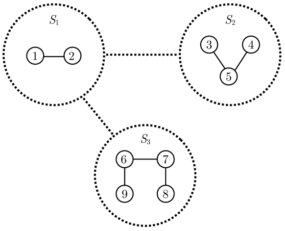
Figure 2: Visualisation of a graph sphere. The dashed circles and lines represent supernodes and superedges, respectively, of a supergraph $G^{\star}$ consisting of the $K=3$ supernodes $S_{1}$, $S_{2}$ and $S_{3}$. Within each supernode, the solid circles and solid lines show the tree among the original variables.

2.3 Data-coherent size-biased tessellation prior

The prior $p(\mathcal{T})$ belongs to the class of data-dependent priors, building on ideas from Voronoi tessellations (Denison et al., 2002a, ; Denison et al., 2002b, ), exchangeable sequences of clusters (ESC, Betancourt et al.,, 2022) and product partition models with covariates (PPMx, Müller et al.,, 2011).

2.3.1 Voronoi tessellation

Our aim is that variables in a supernode refer to the same underlying phenomenon. Specifically, we expect variables in a supernode to be highly correlated as a result of the latent feature. Thus, we enforce such structure in ${\mathcal{T}}$ through a tessellation. In a Voronoi tessellation, elements of a space are grouped together based on their distance to a set of centres. In more details, each centre corresponds to a region. Then, the regions are defined by assigning the elements of the space to the centre they are closest to in terms of some distance.

In our context, the space is the set of nodes $V$ and each region corresponds to a supernode. For a set of centres $C\subset V$, each node is assigned to its closest centre in terms of a distance based on correlation. Denote the (sample) correlation between variables $X_{i},X_{j}$ by

$$\hat{\rho}_{ij}=\frac{X_{i}^{\top}X_{j}}{\|X_{i}\|\,\|X_{j}\|}$$ (1)

Then, node $i$ is assigned to the centre $c\in C$ that minimises the distance metric $\sqrt{2(1-|\hat{\rho}_{ic}|)}$ (Chen et al.,, 2023). Thus, given the distance, $C$ identifies the tessellation ${\mathcal{T}}$ of nodes in a data-driven manner that encourages high correlation among nodes in a supernode. Here, we slightly abuse terminology by referring to the partition $\mathcal{T}$ of the discrete set $V$ as a tessellation while tessellations are usually defined over continuous spaces. The relation between $C$ and $\mathcal{T}$ is deterministic. The approach can be generalised to probabilistic assignment of nodes to centres based on correlations, for instance to incorporate uncertainty about $\mathcal{T}$ and to allow for partitions that are not tessellations.

We define the model on $\mathcal{T}$ hierarchically through the specification of a distribution on the set of centres $C$. Any node in $V$ can be a centre and any combination of nodes is possible. We assume that there is at least one centre and we set $K=|C|$ as the number of regions/supernodes. Note that, given the discrete nature of $V$, different centre combinations can give rise to the same tessellation $\mathcal{T}$ for a specific set of distances.

2.3.2 Size-biased cohesion function

We build on ideas from exchangeable product partition models to specify a distribution for $C$ and hence on $\mathcal{T}$. As a set of centres $C$ corresponds to only one partition, we use the terms centres and partition interchangeably. In the PPMx, the probability assigned to a partition involves the product of a cohesion function and a similarity function. Typically, the cohesion function is derived from an exchangeable partition probability function (EPPF, Hartigan,, 1990), such as the EPPF of the Dirichlet process or Gibbs-type priors (De Blasi et al.,, 2015), which expresses a priori beliefs on the clustering structure. The similarity function usually exploits additional data information useful in the clustering process, biasing the prior probability of a partition towards clusters of subjects that share common “relevant” features. We defer discussion of the similarity function $f_{\textnormal{sim.}}(\cdot)$ to Section 2.3.3.

As cohesion function $f_{\textnormal{coh.}}(\cdot)$, we opt for an extension to the tessellation case of the ESC prior proposed by Betancourt et al., (2022) which provides additional prior control on cluster sizes. Specifically, we use a probability mass function on all positive integers as in Betancourt et al., (2022). Here, the choice of $f_{\textnormal{coh.}}(\cdot)$ provides control over the size (and consequently the number) of the supernodes. We point out that Betancourt et al., (2022) provide a constructive definition of their prior, while our extension to the graph-sphere context is based on heuristics, leading to less effective control on cluster size (see online Appendix LABEL:ap:size-biased).

For a given tessellation $\mathcal{T}$, let $p_{k}=p_{k}(\mathcal{T})=|S_{k}|$ denote the number of nodes in the $k$^th supernode and let $x_{k}=x_{k}(\mathcal{T},X)$ denote the $n\times p_{k}$ matrix consisting of the columns of $X$ assigned to the $k$^th supernode, i.e. $x_{k}=\{X_{i}\}_{i\in S_{k}}$. Moreover, let $\mathcal{C}(\mathcal{T})$ be the set of those combinations of centres $C$ that induce the same $\mathcal{T}$. Moreover, we have $\binom{p}{K}$ ways of choosing $K$ centres among $p$ nodes, giving rise to the term $\binom{p}{|\mathcal{T}|}$ in (2). Then, the prior is defined by

$$p(\mathcal{T})\propto|\mathcal{C}(\mathcal{T})|\,\binom{p}{|\mathcal{T}|}^{-1}\prod_{k=1}^{|\mathcal{T}|}f_{\textnormal{coh.}}\{p_{k}(\mathcal{T})\}\,f_{\textnormal{sim.}}\{x_{k}(\mathcal{T},X)\}$$ (2)

We refer to the prior $p(\mathcal{T})$ as the data-coherent size-biased tessellation prior. Finally, we can formalise how (2) biases the supernode sizes $p_{k}$ if $f_{\textnormal{coh.}}(\cdot)$ is a Geometric distribution with success probability $\pi$.

Proposition 1.

Let $f_{\textnormal{sim.}}(x_{k})=1$ and $f_{\textnormal{coh.}}(p_{k})=(1-\pi)^{p_{k}-1}\,\pi$ in (2). Then, a priori:

1. $p(K)\propto\{\pi/(1-\pi)\}^{K}$

2. Let $E$ denote the expectation w.r.t. the prior and $\overline{p}=\sum_{k=1}^{K}p_{k}/K$ the average supernode size. Then, $E[\overline{p}]$ is a decreasing function of $\pi$ with $E[\overline{p}]\to p$ as $\pi\to 0$ and $E[\overline{p}]\to 1$ as $\pi\to 1$.

Proof.

See online Appendix LABEL:ap:proofs. ∎

As such, a cohesion function that assigns larger values $f_{\textnormal{coh.}}(p_{k})$ to small supernode sizes, e.g. $p_{k}=1$, induces a prior on $\mathcal{T}$ that prefers more and smaller supernodes.

2.3.3 Tree activation function

For the similarity $f_{\textnormal{sim.}}(x_{k})$ in the data-coherent size-biased tessellation prior (2), we choose a function that favours correlated variables to be grouped together, hence encouraging the supernodes to capture large-scale, latent features. We set $f_{\textnormal{sim.}}(x_{k})=\widetilde{p}(x_{k})$, where $\widetilde{p}(x_{k})$ is a probability distribution. We refer to $\widetilde{p}(x_{k})$ as tree activation function and show that such distribution is able to effectively summarise the strength of pairwise correlations in $x_{k}$.

As in the PPMx literature, we set the similarity function to coincide with a probability distribution for computational convenience (see Section 3). Within each region of the tessellation $S_{k}$, we assume that the dependence structure among the variables $x_{k}$ is described by a tree. Then, $\widetilde{p}(x_{k})$ is defined through a standard GGM, but imposing a tree structure on the graph. That is, let $\Delta_{k}$ denote a precision matrix and $x_{ik}$ a row of $x_{k}$. We assume

$$\widetilde{p}(x_{k}\mid\Delta_{k}) =\prod_{i}\mathcal{N}(x_{ik}\mid 0_{p_{k}\times 1},\,\Delta_{k}^{-1})$$

$$\widetilde{p}(x_{k}) =\sum_{T_{k}}\widetilde{p}(T_{k})\int\widetilde{p}(x_{k}\mid\Delta_{k})\,\widetilde{p}(\Delta_{k}\mid T_{k})\,d\Delta_{k}=\sum_{T_{k}}\widetilde{p}(T_{k})\,\widetilde{p}(x_{k}\mid T_{k})$$

The tree $T_{k}=(S_{k},E_{k})$ constrains $\Delta_{k}$ such that $(i,j)\in E_{k}$ if and only if the element of $\Delta_{k}$ corresponding to $i$^th and $j$^th variable in $x_{k}$ is non-zero. Since we assume a tree structure, $\widetilde{p}(\Delta_{k}\mid T_{k})$ is taken to be a Hyper Inverse Wishart distribution (Dawid & Lauritzen,, 1993) with degrees of freedom $\delta>0$ and positive-definite rate matrix $D$. In this case, each edge is a (maximal) clique and each node is a separator. As distribution on $T_{k}$, we consider the uniform distribution over all trees. That is $\widetilde{p}(T_{k})=p_{k}^{2-p_{k}}$ since there are $p_{k}^{p_{k}-2}$ trees on $p_{k}$ nodes (Cayley,, 1889). The restriction to trees is desirable for two reasons. Firstly, an explicit evaluation of $\widetilde{p}(x_{k})$ is feasible (Meilă & Jaakkola,, 2006; Schwaller et al.,, 2019). Secondly, we show that $\widetilde{p}(x_{k})$ accurately captures the correlations in $x_{k}$ as $\widetilde{p}(x_{k}\mid T_{k})$ turns out to be the product of edgewise terms which are a function of pairwise correlations. Let $D_{\{i,j\}}$ be the $2\times 2$ submatrix of $D$ with rows and columns indexed by $\{i,j\}\subset S_{k}$, and

$$g_{ij}(\delta,D)=\frac{\Gamma\{(\delta+1)/2\}\,(D_{ii}D_{jj})^{\delta/2}}{\Gamma(\delta/2)\,|D_{\{i,j\}}|^{(\delta+1)/2}}$$

Define the weights $w_{ij}=g_{ij}(\delta^{\star},D^{\star})/g_{ij}(\delta,D)$ where $\delta^{\star}=\delta+n$ and $D^{\star}=D+X^{\top}X$. Consider a weighted graph with edge weight $w_{ij}$ between nodes $i,j\in S_{k}$. Then, the Laplacian matrix corresponding to the weighted graph is the $p_{k}\times p_{k}$ matrix $\Lambda$ defined by $\Lambda_{ij}=-w_{ij}$ for $i\neq j$ and $\Lambda_{ii}=\sum_{j\neq i}w_{ij}$. Let $\Lambda^{\nu}$ denote the matrix obtained by removing the rows and columns indexed by $\nu\subset S_{k}$ from $\Lambda$.

The following result, which derives from Schwaller et al., (2019), shows in (i–ii) how $\widetilde{p}(x_{k})$ is a function of $w_{ij}$ and in (iii) how to efficiently compute $\widetilde{p}(x_{k})$.

Proposition 2.

1. The tree activation function is equal to

   $$\widetilde{p}(x_{k})=\frac{p_{k}^{2-p_{k}}\,\Gamma(\delta^{\star}/2)^{p_{k}}\,(\prod_{i\in S_{k}}D_{ii})^{\delta/2}}{\pi^{np_{k}/2}\,\Gamma(\delta/2)^{p_{k}}\,(\prod_{i\in S_{k}}D_{ii}^{\star})^{\delta^{\star}/2}}\sum\nolimits_{E_{k}}\prod\nolimits_{(i,j)\in E_{k}}w_{ij}$$

   where the sum is over all edge sets $E_{k}$ such that $T_{k}=(S_{k},E_{k})$ is a tree.

2. $\widetilde{p}(x_{k})$ is an increasing function of any weight $w_{ij}$.

3. For any $u\in S_{k}$, $\sum_{E_{k}}\prod_{(i,j)\in E_{k}}w_{ij}=|\Lambda^{\{u\}}|$ where $\Lambda$ is the Laplacian of the graph with edge weights $w_{ij}$.

Proof.

See online Appendix LABEL:ap:proofs. ∎

The weight $w_{ij}$ is a proxy for the correlation $\hat{\rho}_{ij}$ in (1). Consider the (improper) hyperparameter choice $D=0_{p_{k}\times p_{k}}$. Then,

$$w_{ij}\propto g_{ij}(\delta^{\star},D^{\star})\propto\frac{(D^{\star}_{ii}D^{\star}_{jj})^{\delta^{\star}/2}}{|D^{\star}_{\{i,j\}}|^{(\delta^{\star}+1)/2}}=\frac{(1-\hat{\rho}_{ij}^{2})^{-(\delta^{\star}+1)/2}}{\|X_{i}\|\,\|X_{j}\|}$$

This suggests that $w_{ij}$ and thus $\widetilde{p}(x_{k})$ are increasing functions of the absolute correlation between $X_{i}$ and $X_{j}$. Hence, $\widetilde{p}(x_{k})$ summarises the strength of all correlations in the data.

To provide further insight into the role of $w_{ij}$ in the tree activation function, we focus on the tree edge inclusion probabilities conditionally on $x_{k}$, $\widetilde{\mathrm{Pr}}[{(i,j)\in E_{k}}\mid x_{k}]$. We express $\widetilde{\mathrm{Pr}}[(i,j)\in E_{k}\mid x_{k}]$ in terms of $w_{ij}$, extending a result by Kirshner, (2007). We do so using the resistance distance $r(i,j)$ between nodes $i$ and $j$ in a graph with nodes $S_{k}$ and edge weights $w_{ij}$ (Bapat,, 2004):

$$r(i,j)=\frac{|\Lambda^{\{i,j\}}|}{|\Lambda^{\{i\}}|}$$

where $\Lambda$ is the Laplacian corresponding to the weighted graph (Ali et al.,, 2020).

Proposition 3.

We have:

1. $\widetilde{\mathrm{Pr}}[(i,j)\in E_{k}\mid x_{k}]=w_{ij}\,r(i,j)$

2. $\widetilde{\mathrm{Pr}}[(i,j)\in E_{k}\mid x_{k}]$ is an increasing function of $w_{ij}$.

Proof.

See online Appendix LABEL:ap:proofs. ∎

Therefore, edge activation, i.e. having an inclusion probability above a certain threshold, depends on $w_{ij}$ being large enough. This interpretation of $w_{ij}$ further highlights that the tree activation function $\widetilde{p}(x_{k})$ captures the strength of the dependencies among the variables in the $k$^th supernode. We conclude this section by noting that we could have used a Multivariate $t$-distribution for $\widetilde{p}(x_{k})$, which would allow us to capture global multicollinearity among the variables. We stress that we are interested in understanding the conditional independence structure within a supernode and therefore we opt for a more complex model.

2.4 Supergraph likelihood

Given a tessellation ${\mathcal{T}}$, we specify the supergraph likelihood involving (i) extraction of a latent feature from each supernode and (ii) a GGM on these latent features.

2.4.1 Latent feature extraction

The data-coherent size-biased tessellation prior aims to group highly correlated variables into the same supernode. To summarise the latent feature, captured by each supernode, we compute the first PC of $x_{k}$. Such use of principal component analysis (PCA) as a dimensionality reduction tool is supported by empirical and theoretical results (Meyer,, 1975; Malevergne & Sornette,, 2004; Stepanov et al.,, 2021; Whiteley et al.,, 2022).

Let $\phi$ denote the proportion of variance in $x_{k}$ explained by the first PC of $x_{k}$. Let $\rho$ be the average correlation, $s^{2}$ the average squared correlation in the $k$^th supernode and $\rho^{i}$ the average absolute correlation of variable $i$, with

$$\rho =\frac{2}{p_{k}(p_{k}-1)}\sum_{i>j\in S_{k}}\hat{\rho}_{ij}$$

$$s^{2} =\frac{2}{p_{k}(p_{k}-1)}\sum_{i>j\in S_{k}}\hat{\rho}_{ij}^{2}$$

$$\rho^{i} =\frac{1}{p_{k}-1}\sum_{j\in S_{k}:j\neq i}|\hat{\rho}_{ij}|$$

Following Stepanov et al., (2021), we can show the following proposition.

Proposition 4.

Let

$$h_{p_{k}}(t) =\frac{1}{p_{k}}+\left(1-\frac{1}{p_{k}}\right)t$$

$$h_{\star}(t) =\begin{cases}\tfrac{1}{2}(1+\sqrt{2t-1}),\quad&t\geq\tfrac{1}{2}\\ t,&\text{otherwise}\end{cases}$$

The proportion $\phi$ of variance explained by the first principal component satisfies:

1. $\max[h_{p_{k}}(\rho),\,h_{\star}\{h_{p_{k}}(s^{2})\}]\leq\phi\leq\min\{h_{p_{k}}(s),\,\max_{i}h_{p_{k}}(\rho^{i})\}$

2. If all correlations $\hat{\rho}_{ij}$ are equal, then

   $$\phi=\begin{cases}h_{p_{k}}(\rho),\quad&\rho\geq 0\\ \frac{1-\rho}{p},\quad&\text{otherwise}\end{cases}$$

Proof.

See online Appendix LABEL:ap:proofs. ∎

Thus, higher absolute correlations in $x_{k}$ imply that the first PC is able to better describe most of the variation in a supernode. Moreover, with perfect correlations ($s^{2}=1$), the first PC captures all variation in $x_{k}$. See also Figure LABEL:fig:prop_var in Supplementary Material.

2.4.2 Model on the latent features

We now specify a GGM that links the supernodes through their latent features. What follows is conditional on a tessellation with $K$ regions and supernodes $\{S_{k}\}$. Let the $n\times K$ matrix $Y^{\star}$ contain the first PCs corresponding to each supernode $x_{k}$. The PCs are standardised such that $\|Y^{\star}_{k}\|^{2}=n$. As model for $Y^{\star}$, we assume a GGM, where each row of $Y^{\star}$ is normally distributed with mean zero and precision matrix $\Omega^{\star}$ conditionally on the supergraph $G^{\star}$.

2.4.3 Augmented space

In the previous subsection, we have defined the model for the supergraph conditional on the tessellation. We note that the focus of inference is not only on the supergraph but also on the tessellation of nodes. This includes also inference on $K$ as well as each supernode composition $S_{k}$. As such, when performing posterior inference using Markov chain Monte Carlo (MCMC) methods, this often would require transdimensional moves and consequentially devising labour-intensive MCMC schemes since $Y^{\star}$ changes dimension with $K$ and supernode membership changes with tessellation. This issue will be discussed more exhaustively in Section 3.3. Note that such changes in dimensions are different from those addressed by tools such as reversible jump MCMC (Green,, 1995) where the parameter instead of the data changes dimension. Thus, to avoid the change in dimension, we resort to a data augmentation trick, which has been successfully exploited in other contexts (e.g. Royle et al.,, 2007; Walker,, 2007). We define a GGM on an augmented space which has the same dimension $p$ as the original data $X$. We specify a GGM on all $p$ PCs across the supernodes instead of on just the $K$ first PCs. Note that if a supernode contains $p_{k}$ variables, then the number of PCs associated to $S_{k}$ is $p_{k}$ with $\sum_{k=1}^{K}p_{k}=p$. Therefore, let $Y$ denote the $n\times p$ matrix obtained by adding all lower ranked PCs to $Y^{\star}$, again standardised such that $\|Y_{i}\|^{2}=n$ for every $i$. We highlight that our interest is uniquely in the links among supernodes, i.e. between first PCs, rather than in any weaker patterns involving lower ranked PCs. Such a focus is also indispensable for a reduction in complexity in terms of GGM inference as well as interpretation. Let $G$ be a graph on $p$ nodes where edges (corresponding to superedges) can only exist between the $K$ nodes corresponding to first PCs such that the supergraph $G^{\star}$ uniquely determines $G$. The other $(p-K)$ nodes are auxiliary to avoid changes in dimension. Such use of an augmented parameter $G$ is similar in spirit to the use of pseudopriors by Carlin & Chib, (1995). They also consider the use of auxiliary parameters to avoid transdimensionality in their MCMC.

In more details, let the rows of $Y$ be independently distributed according to $\mathcal{N}(0_{p\times 1},\,\Omega^{-1})$. Conditionally on the graph $G$, the prior on the precision matrix $\Omega$ is the $G$-Wishart distribution with degrees of freedom $\delta_{G}>0$ and positive-definite rate matrix $D_{G}$. Note that nodes corresponding to lower ranked PCs are not connected among themselves or with any supernode. As such there will always be a zero element in the precision matrix in such entries. This gives rise to the marginal likelihood (e.g. Atay-Kayis & Massam,, 2005)

$$p(Y^{\star}\mid\mathcal{T},G^{\star},X)\propto p(Y\mid\mathcal{T},G,X)=\frac{I_{G}(\delta_{G}^{\star},D_{G}^{\star})}{(2\pi)^{np/2}I_{G}(\delta_{G},D_{G})}$$ (3)

where $\delta_{G}^{\star}=\delta_{G}+n$, $D_{G}^{\star}=D_{G}+Y^{\top}Y$, and $I_{G}(\delta_{G},D_{G})$ denotes the normalising constant of the density of the $G$-Wishart distribution with graph $G$, degrees of freedom $\delta_{G}$ and rate matrix $D_{G}$. Note that $p(Y\mid\mathcal{T},G,X)$ depends only on $Y^{\star}$ and not on the lower ranked PCs $(Y\setminus Y^{\star})$ due to standardisation. Furthermore, the induced precision matrix $\Omega^{\star}$ of $Y^{\star}$ corresponds to $G^{\star}$. In what follows, with abuse of terminology, we refer to $G$ as supergraph as $G^{\star}$ can be deterministically recovered from $G$. Finally, a choice of prior $p(G\mid\mathcal{T})$ on supergraphs, which we discuss in Section 4, completes the model specification.

3 Inference

Main object of inference are the tessellation $\mathcal{T}$ and the supergraph $G$, from which we can recover $G^{\star}$. The target distribution is

$$p(\mathcal{T},G,Y\mid X)\propto p(\mathcal{T})\,p(G\mid\mathcal{T})\,p(Y\mid\mathcal{T},G,X)$$ (4)

Sampling from the distribution in (4) enables posterior inference on the graph sphere $(\mathcal{T},G^{\star})$. Many challenges need to be addressed to sample from this distribution. First of all, we have $n$ observations for each of the $p$ nodes. As a result, the posterior on the tessellation is highly concentrated unless $n$ is small: see online Appendix LABEL:ap:conc where we show that $p(\mathcal{T}\mid X)$ can be a point mass for moderate $n$. We remark that the approaches for clustering of nodes by Peixoto, (2019) and van den Boom et al., 2022b do not suffer from this collapsing of the posterior on the partition as $n$ gets large. That is because they cluster nodes based on edges in the graph, with the graph representing a single (latent) observation. In their set-up, a large $n$ results in concentration of the posterior on the graph but typically not of the posterior on the partition.

Such concentration of $p(\mathcal{T}\mid X)$ inhibits MCMC convergence and mixing. To still be able to use MCMC for inference, we consider transformations of the posterior in (4) that are less concentrated. Specifically, we propose two possible solutions: (i) coarsening of the tree activation functions and the likelihood; (ii) nested MCMC with coarsening of the tree activation functions. A coarsened likelihood is a likelihood raised to a power as in Page & Quintana, (2018), with the goal of flattening it for better exploration of posterior space.

3.1 Coarsening of the tree activation functions

The tree activation function $\widetilde{p}(x_{k})$, defined as a probability distribution in Section 2.3.3, generally becomes more peaked as the sample size $n$ increases. More specifically, $\widetilde{p}(x_{k})$ is defined through the conditional distribution $\widetilde{p}(x_{k}\mid T_{k})$ with tree $T_{k}=(S_{k},E_{k})$, where the $n$ rows of $x_{k}$ are independently distributed conditionally on the precision $\Delta_{k}$. This scaling with $n$ results in the prior $p(\mathcal{T})$ with the similarity function $f_{\textnormal{sim.}}(x_{k})=\widetilde{p}(x_{k})$ to be skewed too strongly by the similarity information for large sample sizes. Then, the size biasing from the cohesion function $f_{\textnormal{coh.}}(\cdot)$ in (2) becomes negligible, and $p(\mathcal{T})$ becomes too peaked.

A similar phenomenon appears in PPMx if the number of covariates increases with the partition prior becoming very peaked (Barcella et al.,, 2017), and the posterior concentrating on on either $K=1$ or $K=p$ clusters as the dimensionality increases (Chandra et al.,, 2023). Relatedly, the prior in PPMx with many covariates may dominate the posterior distribution with the likelihood being much less peaked than the prior. A variety of solutions have been explored to address this issue (Page & Quintana,, 2018) including dimensionality reduction via covariate selection and enrichment with clustering at two levels (Wade et al.,, 2014).

The issue of a too concentrated prior is yet more pertinent in our context because we cluster variables/nodes while PPMx consider clustering of observations. Thus, the tree activation functions dominate when the sample size is large. Also, we treat the observations as exchangeable such that approaches based on variable selection or enrichment are not sensible. Instead, as in Page & Quintana, (2018), we coarsen the similarity functions.

We use a modified $\widetilde{p}(x_{k})$ as similarity function $f_{\textnormal{sim.}}(x_{k})$: we replace the distribution $\widetilde{p}(x_{k}\mid T_{k})$ by the coarsened version $\widetilde{p}(x_{k}\mid T_{k})^{\zeta}$ for some power $\zeta\in(0,1]$. We consider $\zeta\propto n^{-1}$ to reflect the $n$ i.i.d. observations. The power balances how strongly the correlations in $X$ inform the tessellation. Specifically, instead of $f_{\textnormal{sim.}}(x_{k})=\widetilde{p}(x_{k})=\sum_{T_{k}}\widetilde{p}(x_{k}\mid T_{k})\,\widetilde{p}(T_{k})$, we use the coarsened similarity function

$$f_{\textnormal{sim.}}^{(\zeta)}(x_{k})=\sum_{T_{k}}\widetilde{p}(x_{k}\mid T_{k})^{\zeta}\,\widetilde{p}(T_{k})$$ (5)

where the sum is over all possible $T_{k}$ and $\widetilde{p}(T_{k})=p_{k}^{2-p_{k}}$ is the uniform distribution. This prior choice facilitates the computation of the similarity function, as computation of $\widetilde{p}(x_{k})$ via the determinant $|\Lambda^{\{u\}}|$ in Proposition 2 is notoriously numerically unstable (Momal et al.,, 2021). This is due to the relative sizes of the weights $w_{ij}$ diverging as $n$ and $p_{k}$ increase. To alleviate the problem, we can replace $w_{ij}$ by $w_{ij}^{\zeta}$ in Proposition 2 to compute $f_{\textnormal{sim.}}^{(\zeta)}(x_{k})$ instead of $\widetilde{p}(x_{k})$.

With regard to the choice of the power $\zeta$, Page & Quintana, (2018) use $\zeta=n^{-1}$, though coarsening with larger powers, still with $\zeta\to 0$ as $n\to\infty$, has been explored within PPMx (Pedone et al.,, 2023) and in other contexts (Miller & Dunson,, 2019). Alternatively, a prior can be placed on $\zeta$ as it has been done in the context of power priors (Chen & Ibrahim,, 2000). MCMC with a prior on $\zeta$ is challenging as it leads to a doubly intractable posterior (Carvalho & Ibrahim,, 2021). We further discuss our choice of $\zeta$ in Section 4.

3.2 Coarsening of the likelihood and nested MCMC

Like the tree activation function, the information provided by the supergraph likelihood $p(Y\mid\mathcal{T},G,X)$ in (3) scales with the sample size $n$. Also this scaling causes posterior uncertainty for the tessellation $\mathcal{T}$ to vanish for large $n$. To counterbalance this phenomenon, we consider two options: coarsening of the likelihood and nested MCMC.

3.2.1 Coarsening of the likelihood

Coarsening or flattening the likelihood can undo its undesirable scaling with $n$. However, there is a need to balance the information provided by the similarity function $f_{\textnormal{sim.}}^{(\zeta)}(\cdot)$ and by the likelihood. Therefore, we use the same power $\zeta$ to coarsen both the tree activation functions and the likelihood. Specifically, we use a transformation of the posterior in (4) as target distribution:

$$\pi^{(\zeta)}(\mathcal{T},G,Y)\propto p^{(\zeta)}(\mathcal{T})\,p(G\mid\mathcal{T})\,p(Y\mid\mathcal{T},G,X)^{\zeta}$$ (6)

where $p(Y\mid\mathcal{T},G,X)^{\zeta}$ is the likelihood raised to the power $\zeta$ and $p^{(\zeta)}(\mathcal{T})$ is the data-coherent size-biased tessellation prior in (2) with the coarsened $f_{\textnormal{sim.}}^{(\zeta)}(\cdot)$ in (5) as similarity function.

As in the context of model misspecification, raising the likelihood to a power is done to avoid undesired concentration of the posterior (e.g. Grünwald & van Ommen,, 2017; Miller & Dunson,, 2019). Furthermore, such a power is standard in Gibbs posteriors where the likelihood derives from a loss function and the power balances the influence of the prior (e.g. Jiang & Tanner,, 2008). Finally, Martin et al., (2017) and Liu et al., (2021) coarsen the likelihood to avoid overconcentration of the posterior with data-coherent priors.

3.2.2 Nested MCMC

An alternative to coarsening of the likelihood to avoid overconcentration of the posterior is to recast the problem within cutting feedback (Plummer,, 2015), cutting the feedback from $Y$ to $\mathcal{T}$ such that $Y$ does not inform $\mathcal{T}$. The target becomes the cut distribution

$$\pi_{\textnormal{cut}}(\mathcal{T},G,Y)\propto p^{(\zeta)}(\mathcal{T})\,p(G,Y\mid\mathcal{T},X)$$ (7)

where $p(G,Y\mid\mathcal{T},X)\propto{p(G\mid\mathcal{T})}\,{p(Y\mid\mathcal{T},G,X)}$ is the posterior on the supergraph conditionally on $\mathcal{T}$. Then, the marginal distribution on $\mathcal{T}$ under the target is $p^{(\zeta)}(\mathcal{T})$ which is sufficiently diffuse under enough coarsening, i.e. small enough $\zeta$. To sample $\pi_{\textnormal{cut}}(\mathcal{T},G,Y)$, we use nested MCMC (Plummer,, 2015; Carmona & Nicholls,, 2020) which allows for parallel computation. We note that the cut posterior in (7) is an approximation of the true posterior.

We employ cutting feedback to improve MCMC mixing (see also Liu et al.,, 2009; Plummer,, 2015). Moreover, a random variable whose feedback is being cut might provide information about a parameter that conflicts with other, more trusted parts of the model (Plummer,, 2015; Jacob et al.,, 2017). Such a conflict is present here: the information in $p(Y\mid\mathcal{T},G,X)$ provides contrasting information for the tessellation as compared to the data-coherent size-biased tessellation prior.

3.3 Posterior computation

We perform posterior inference by drawing either from $\pi^{(\zeta)}(\mathcal{T},G,Y)$ or $\pi_{\textnormal{cut}}(\mathcal{T},G,Y)$. In both cases, we need to devise tailored computational solutions, which, nevertheless, exploit the same techniques. The resulting algorithms are detailed in online Appendix LABEL:ap:mcmc. Firstly, recall from Section 2.3.1 that the tessellation $\mathcal{T}$ is a deterministic function of the set of centres $C$. For convenience, we choose to work directly with $C$ instead of $\mathcal{T}$ in the MCMC.

Working with $C$, we employ both birth-death and move Metropolis-Hastings steps. The birth-death step uses as proposal the addition or removal of an element from $C$, which results in a restructuring of the supernodes configuration. These changes in $C$ are accompanied by corresponding Metropolis-Hastings proposals for $G$. Additionally, keeping the number of centres fixed, we propose to move a centre from one node to another, which does not require a change in $G$ (although supernode membership might change).

For improved Metropolis-Hastings proposals for the birth-death steps, which involve both $C$ and $G$, we consider locally balanced informed proposals (Zanella,, 2019), which enable parallel computations. To limit the computational cost associated with the informed proposals, we constrain the neighbourhood of values for $(C,G)$ that such a proposal considers (see online Appendix LABEL:ap:mcmc for details).

4 Application to gene expression data

In online Appendix LABEL:ap:simul, we present simulation studies to investigate the performance of the graph sphere model and show that coarsening of the likelihood and nested MCMC can result in different inference. We discuss the differences and the relative merits of both approaches in terms of recovery of large-scale structure. Here, we apply our methodology to gene expression levels, the interactions between which are often represented as networks. An important concept in the gene network literature is that of module, which is a densely connected subgraph of genes with similar expression profiles (Zhang,, 2018). Such genes are typically co-regulated and functionally related (Saelens et al.,, 2018). Therefore, a critical step in the analysis of large gene expression data sets is module detection with the goal of grouping genes into co-expression clusters. The graph sphere model treats each module as a supernode and has intrinsic advantages to learn the supernode/module membership from data. On the other hand, in the gene network literature, typically, a two-step approach is adopted. First the graph is estimated from the gene expressions, and then the modules are derived from the graph estimate (see, e.g., Saelens et al.,, 2018; Zhang,, 2018). Such an approach underestimates uncertainty, often leading to false positives, and does not capture the mesoscopic dependency structure between modules.

We analyse data on gene expressions from $n=561$ ovarian cancer tissue samples from The Cancer Genome Atlas. We focus on $p=373$ genes identified in Table 2 of Zhang, (2018) as spread across six estimated modules which are highly enriched in terms of Gene Ontology (GO, Ashburner et al.,, 2000) annotations. The gene expressions are quantile-normalised to marginally follow a standard Gaussian distribution. We apply the proposed graph sphere methodology with the following prior specification. Like Betancourt et al., (2022), we opt for a shifted Negative Binomial distribution starting at $p_{k}=1$ as cohesion function $f_{\textnormal{coh.}}(p_{k})$ in the tessellation prior. As hyperparameters of the Negative Binomial distribution, we choose a success probability of $1/6$ and a size parameter of $2$, with an expected supernode size equal to 10 based on an initial exploratory data analysis. Hyperparameters for the Hyper Inverse Wishart distribution $\widetilde{p}(\Delta_{k}\mid T_{k})$ in the tree activation function and the $G$-Wishart prior $p(\Omega\mid G)$ for the supergraph are set to the standard values $\delta=3$, $D=I_{p_{k}}$, $\delta_{G}=3$ and $D_{G}=I_{p}$. We specify a uniform prior for the supergraph, i.e. $p(G\mid\mathcal{T})=2^{-K(K-1)/2}$, as it improves MCMC mixing by flattening the posterior (see online Appendix LABEL:ap:mcmc for a discussion). Finally, the coarsening parameter $\zeta$ is chosen small enough ($\zeta=10/n$) to allow for good MCMC mixing without flattening the target distribution excessively. We run both MCMC algorithms for 110000 iterations, discarding the first 10000 as burn-in.

The inference on the tessellation (see online Appendix LABEL:ap:gene and Figure 1) reveals a more refined grouping of genes into supernodes than the modules estimated by Zhang, (2018) but the partition of genes is otherwise similar, both with coarsening of the likelihood and with nested MCMC. Here, we report the tessellation that minimises the lower bound to the posterior expectation of the variation of information (Wade & Ghahramani,, 2018). This results in, respectively, $K=72$ and $24$ supernodes with coarsening of the likelihood and nested MCMC. We note the difference in the number of supernodes obtained with the two algorithms. Recall that the nested MCMC does not allow for information transfer from the supergraph to the tessellation. The supergraph likelihood is obviously favouring more structure in the data. Still, examining the supernodes obtained with the two methods, we note that the 72 supernodes are congruent with the 24, in the sense that most of the 72 supernodes are contained in only one of the 24 supernodes.

We visualise the resulting graph sphere in Figure 1 (in Section 1) only for nested MCMC, as its smaller $K$ makes for easier exposition than the larger $K$ with the coarsened likelihood. The trees $T_{k}$ shown are those that maximise $\widetilde{p}(T_{k}\mid x_{k})$ in the tree activation functions obtained using a maximum spanning tree algorithm (Schwaller et al.,, 2019). For comparison, consider Module 14 from Zhang, (2018), which is the only module that we include for which Zhang, (2018) reports edge estimates. All but one edge between genes from Module 14 in Figure 1 are also inferred by Zhang, (2018), which suggests that the inference on trees is appropriate. For the supergraph, we draw from the posterior $p(G\mid\mathcal{T},X)$ with the tessellation $\mathcal{T}$ fixed to the point estimate using the GGM MCMC methodology from van den Boom et al., 2022a , resulting in 109 superedges (approximately half of the possible edges) with a posterior inclusion probability greater than $0.5$. For visualisation purposes, we include fewer superedges in Figure 1, i.e. only those with a posterior probability greater than 0.99. Again, there is consistency with the modules estimated by Zhang, (2018): each supernode corresponds to a single module as the vast majority of its nodes, if not all, come from the same module. Note that 35% of all pairs of supernodes that both correspond to the same module are connected by a superedge in Figure 1. This drops to 18% for pairs corresponding to different modules. In online Appendix LABEL:ap:gene, we furthermore find that the presence of a superedge is associated with more interactions as derived from the STRING database (Szklarczyk et al.,, 2021) between pairs of genes involved in the two linked supernodes, suggesting biological meaning of the superedge inference. Finally, such interactions are much more prevalent within supernodes than between, which indicates that our more granular partition of nodes compared to Zhang, (2018) is justified.

To further inspect the tessellations, we perform GO over-representation analysis in online Appendix LABEL:ap:gene. Such analysis detects GO terms that appear relatively more frequently among the genes in a supernode than among all 373 genes. We summarise the results in Figure LABEL:fig:GO in Supplementary Material. We find that different supernodes are generally associated with distinct biological processes (i.e. GO terms), suggesting that our model is able to capture underlying biological mechanisms.

SUPPLEMENTARY MATERIAL

Supplement:

Simulation studies, overview of notation and related work, further material on the size-biased prior and the gene expression application, proofs of the propositions, and details of the MCMC algorithms. (.pdf file)

Code:

The code to implement the model is available at https://github.com/willemvandenboom/graph-sphere. (GitHub repository)

ACKNOWLEDGEMENTS

The data used in Section 4 are generated by The Cancer Genome Atlas Research Network: https://www.cancer.gov/tcga.

References

- Ali et al., (2020) Ali, P., Atik, F., & Bapat, R. B. (2020). Identities for minors of the Laplacian, resistance and distance matrices of graphs with arbitrary weights. Linear and Multilinear Algebra, 68(2):323–336.
- Ashburner et al., (2000) Ashburner, M., Ball, C. A., Blake, J. A., Botstein, D., Butler, H., Cherry, J. M., et al. (2000). Gene Ontology: tool for the unification of biology. Nature Genetics, 25(1):25–29.
- Atay-Kayis & Massam, (2005) Atay-Kayis, A. & Massam, H. (2005). A Monte Carlo method for computing the marginal likelihood in nondecomposable Gaussian graphical models. Biometrika, 92(2):317–335.
- Bapat, (2004) Bapat, R. B. (2004). Resistance matrix of a weighted graph. MATCH Communications in Mathematical and in Computer Chemistry, 50:73–82.
- Barabási, (2012) Barabási, A.-L. (2012). The network takeover. Nature Physics, 8(1):14–16.
- Barabási, (2016) Barabási, A.-L. (2016). Network Science. Cambridge University Press, Cambridge, England.
- Barcella et al., (2017) Barcella, W., De Iorio, M., & Baio, G. (2017). A comparative review of variable selection techniques for covariate dependent Dirichlet process mixture models. Canadian Journal of Statistics, 45(3):254–273.
- Betancourt et al., (2022) Betancourt, B., Zanella, G., & Steorts, R. C. (2022). Random partition models for microclustering tasks. Journal of the American Statistical Association, 117(539):1215–1227.
- Bhadra et al., (2019) Bhadra, A., Datta, J., Polson, N. G., & Willard, B. (2019). Lasso meets horseshoe: a survey. Statistical Science, 34(3):405–427.
- Bock & Gibbons, (2021) Bock, R. D. & Gibbons, R. D. (2021). Item Response Theory. Wiley, Hoboken, NJ.
- Carlin & Chib, (1995) Carlin, B. P. & Chib, S. (1995). Bayesian model choice via Markov chain Monte Carlo methods. Journal of the Royal Statistical Society: Series B (Methodological), 57(3):473–484.
- Carmona & Nicholls, (2020) Carmona, C. & Nicholls, G. (2020). Semi-modular inference: enhanced learning in multi-modular models by tempering the influence of components. Proceedings of the Twenty Third International Conference on Artificial Intelligence and Statistics, 4226–4235. PMLR.
- Carvalho & Ibrahim, (2021) Carvalho, L. M. & Ibrahim, J. G. (2021). On the normalized power prior. Statistics in Medicine, 40(24):5251–5275.
- Cayley, (1889) Cayley, A. (1889). A theorem on trees. The Quarterly Journal of Pure and Applied Mathematics, 23:376–378.
- Chandra et al., (2023) Chandra, N. K., Canale, A., & Dunson, D. B. (2023). Escaping the curse of dimensionality in Bayesian model-based clustering. Journal of Machine Learning Research, 24(144).
- Chen et al., (2023) Chen, J., Ng, Y. K., Lin, L., Zhang, X., & Li, S. (2023). On triangle inequalities of correlation-based distances for gene expression profiles. BMC Bioinformatics, 24:40.
- Chen & Ibrahim, (2000) Chen, M.-H. & Ibrahim, J. G. (2000). Power prior distributions for regression models. Statistical Science, 15(1):46–60.
- Dawid & Lauritzen, (1993) Dawid, A. P. & Lauritzen, S. L. (1993). Hyper Markov laws in the statistical analysis of decomposable graphical models. The Annals of Statistics, 21(3):1272–1317.
- De Blasi et al., (2015) De Blasi, P., Favaro, S., Lijoi, A., Mena, R. H., Prunster, I., & Ruggiero, M. (2015). Are Gibbs-type priors the most natural generalization of the Dirichlet process? IEEE Transactions on Pattern Analysis and Machine Intelligence, 37(2):212–229.
- Dempster, (1972) Dempster, A. P. (1972). Covariance selection. Biometrics, 28(1):157–175.
- (21) Denison, D., Adams, N., Holmes, C., & Hand, D. (2002a). Bayesian partition modelling. Computational Statistics & Data Analysis, 38(4):475–485.
- (22) Denison, D. G. T., Holmes, C. C., Mallick, B. K., & Smith, A. F. M. (2002b). Bayesian methods for nonlinear classification and regression. Wiley Series in Probability and Statistics. John Wiley & Sons, Chichester, UK.
- Drovandi et al., (2015) Drovandi, C. C., Pettitt, A. N., & Lee, A. (2015). Bayesian indirect inference using a parametric auxiliary model. Statistical Science, 30(1):72–95.
- Fienberg, (2012) Fienberg, S. E. (2012). A brief history of statistical models for network analysis and open challenges. Journal of Computational and Graphical Statistics, 21(4):825–839.
- Green, (1995) Green, P. J. (1995). Reversible jump Markov chain Monte Carlo computation and Bayesian model determination. Biometrika, 82(4):711–732.
- Grünwald & van Ommen, (2017) Grünwald, P. & van Ommen, T. (2017). Inconsistency of Bayesian inference for misspecified linear models, and a proposal for repairing it. Bayesian Analysis, 12(4):1069–1103.
- Hartigan, (1990) Hartigan, J. (1990). Partition models. Communications in Statistics - Theory and Methods, 19(8):2745–2756.
- Iñiguez et al., (2020) Iñiguez, G., Battiston, F., & Karsai, M. (2020). Bridging the gap between graphs and networks. Communications Physics, 3:88.
- Jacob et al., (2017) Jacob, P. E., Murray, L. M., Holmes, C. C., & Robert, C. P. (2017). Better together? Statistical learning in models made of modules. arXiv:1708.08719v1.
- Jiang & Tanner, (2008) Jiang, W. & Tanner, M. A. (2008). Gibbs posterior for variable selection in high-dimensional classification and data mining. The Annals of Statistics, 36(5):2207–2231.
- Kirshner, (2007) Kirshner, S. (2007). Learning with tree-averaged densities and distributions. Advances in Neural Information Processing Systems. Curran Associates, Inc.
- Knudson & Lindsey, (2014) Knudson, D. V. & Lindsey, C. (2014). Type I and type II errors in correlations of various sample sizes. Comprehensive Psychology, 3:1.
- Lauritzen, (1996) Lauritzen, S. L. (1996). Graphical Models. Oxford Statistical Science Series. The Clarendon Press, Oxford.
- Lewis et al., (2021) Lewis, J. R., MacEachern, S. N., & Lee, Y. (2021). Bayesian restricted likelihood methods: conditioning on insufficient statistics in Bayesian regression (with discussion). Bayesian Analysis, 16(4):1393–1462.
- Liu et al., (2021) Liu, C., Yang, Y., Bondell, H., & Martin, R. (2021). Bayesian inference in high-dimensional linear models using an empirical correlation-adaptive prior. Statistica Sinica, 31:2051–2072.
- Liu et al., (2009) Liu, F., Bayarri, M. J., & Berger, J. O. (2009). Modularization in Bayesian analysis, with emphasis on analysis of computer models. Bayesian Analysis, 4(1):119–150.
- Malevergne & Sornette, (2004) Malevergne, Y. & Sornette, D. (2004). Collective origin of the coexistence of apparent random matrix theory noise and of factors in large sample correlation matrices. Physica A: Statistical Mechanics and its Applications, 331(3–4):660–668.
- Martin et al., (2017) Martin, R., Mess, R., & Walker, S. G. (2017). Empirical Bayes posterior concentration in sparse high-dimensional linear models. Bernoulli, 23(3):1822–1847.
- Martin & Walker, (2019) Martin, R. & Walker, S. G. (2019). Data-driven priors and their posterior concentration rates. Electronic Journal of Statistics, 13(2):3049–3081.
- Meilă & Jaakkola, (2006) Meilă, M. & Jaakkola, T. (2006). Tractable Bayesian learning of tree belief networks. Statistics and Computing, 16(1):77–92.
- Meyer, (1975) Meyer, E. P. (1975). A measure of the average intercorrelation. Educational and Psychological Measurement, 35(1):67–72.
- Miller & Dunson, (2019) Miller, J. W. & Dunson, D. B. (2019). Robust Bayesian inference via coarsening. Journal of the American Statistical Association, 114(527):1113–1125.
- Momal et al., (2021) Momal, R., Robin, S., & Ambroise, C. (2021). Accounting for missing actors in interaction network inference from abundance data. Journal of the Royal Statistical Society Series C: Applied Statistics, 70(5):1230–1258.
- Müller et al., (2011) Müller, P., Quintana, F., & Rosner, G. L. (2011). A product partition model with regression on covariates. Journal of Computational and Graphical Statistics, 20(1):260–278.
- Newman, (2012) Newman, M. E. J. (2012). Communities, modules and large-scale structure in networks. Nature Physics, 8(1):25–31.
- Page & Quintana, (2018) Page, G. L. & Quintana, F. A. (2018). Calibrating covariate informed product partition models. Statistics and Computing, 28(5):1009–1031.
- Pedone et al., (2023) Pedone, M., Argiento, R., & Stingo, F. C. (2023). A Bayesian nonparametric approach to personalized treatment selection. arXiv:2210.06030v2.
- Peixoto, (2019) Peixoto, T. P. (2019). Network reconstruction and community detection from dynamics. Physical Review Letters, 123(12):128301.
- Plummer, (2015) Plummer, M. (2015). Cuts in Bayesian graphical models. Statistics and Computing, 25(1):37–43.
- Pratt, (1965) Pratt, J. W. (1965). Bayesian interpretation of standard inference statements. Journal of the Royal Statistical Society: Series B (Methodological), 27(2):169–192.
- Ravasz et al., (2002) Ravasz, E., Somera, A. L., Mongru, D. A., Oltvai, Z. N., & Barabási, A.-L. (2002). Hierarchical organization of modularity in metabolic networks. Science, 297:1551–1555.
- Rodrigues Jr. et al., (2006) Rodrigues Jr., J., Traina, A. J. M., Faloutsos, C., & Traina Jr., C. (2006). SuperGraph visualization. Eighth IEEE International Symposium on Multimedia (ISM'06). IEEE.
- Roverato, (2002) Roverato, A. (2002). Hyper inverse Wishart distribution for non-decomposable graphs and its application to Bayesian inference for Gaussian graphical models. Scandinavian Journal of Statistics, 29(3):391–411.
- Royle et al., (2007) Royle, J. A., Dorazio, R. M., & Link, W. A. (2007). Analysis of multinomial models with unknown index using data augmentation. Journal of Computational and Graphical Statistics, 16(1):67–85.
- Saelens et al., (2018) Saelens, W., Cannoodt, R., & Saeys, Y. (2018). A comprehensive evaluation of module detection methods for gene expression data. Nature Communications, 9:1090.
- Schwaller et al., (2019) Schwaller, L., Robin, S., & Stumpf, M. (2019). Closed-form Bayesian inference of graphical model structures by averaging over trees. Journal de la Société Française de Statistique, 160(2):1–23.
- Sporns & Betzel, (2016) Sporns, O. & Betzel, R. F. (2016). Modular brain networks. Annual Review of Psychology, 67:613–640.
- Stepanov et al., (2021) Stepanov, Y., Herrmann, H., & Guhr, T. (2021). Generic features in the spectral decomposition of correlation matrices. Journal of Mathematical Physics, 62(8):083505.
- Szklarczyk et al., (2021) Szklarczyk, D., Gable, A. L., Nastou, K. C., Lyon, D., Kirsch, R., Pyysalo, S., et al. (2021). The STRING database in 2021: customizable protein–protein networks, and functional characterization of user-uploaded gene/measurement sets. Nucleic Acids Research, 49(D1):D605–D612.
- (60) van den Boom, W., Beskos, A., & De Iorio, M. (2022a). The -Wishart weighted proposal algorithm: efficient posterior computation for Gaussian graphical models. Journal of Computational and Graphical Statistics, 31(4):1215–1224.
- (61) van den Boom, W., De Iorio, M., & Beskos, A. (2022b). Bayesian learning of graph substructures. Bayesian Analysis. Advance online publication.
- Wade et al., (2014) Wade, S., Dunson, D. B., Petrone, S., & Trippa, L. (2014). Improving prediction from Dirichlet process mixtures via enrichment. Journal of Machine Learning Research, 15(30):1041–1071.
- Wade & Ghahramani, (2018) Wade, S. & Ghahramani, Z. (2018). Bayesian cluster analysis: point estimation and credible balls (with discussion). Bayesian Analysis, 13(2):559–626.
- Walker, (2007) Walker, S. G. (2007). Sampling the Dirichlet mixture model with slices. Communications in Statistics - Simulation and Computation, 36(1):45–54.
- Whiteley et al., (2022) Whiteley, N., Gray, A., & Rubin-Delanchy, P. (2022). Discovering latent topology and geometry in data: a law of large dimension. arXiv:2208.11665v2.
- Yook et al., (2004) Yook, S.-H., Oltvai, Z. N., & Barabási, A.-L. (2004). Functional and topological characterization of protein interaction networks. Proteomics, 4(4):928–942.
- Zanella, (2019) Zanella, G. (2019). Informed proposals for local MCMC in discrete spaces. Journal of the American Statistical Association, 115(530):852–865.
- Zhang, (2018) Zhang, S. (2018). Comparisons of gene coexpression network modules in breast cancer and ovarian cancer. BMC Systems Biology, 12(S1):57–87.