Kernel Learning in Ridge Regression “Automatically” Yields Exact Low Rank Solution

Abstract

We consider kernels of the form $(x,x^{\prime})\mapsto\phi(\left\|{x-x^{\prime}}\right\|^{2}_{\Sigma})$ parametrized by $\Sigma$. For such kernels, we study a variant of the kernel ridge regression problem which simultaneously optimizes the prediction function and the parameter $\Sigma$ of the reproducing kernel Hilbert space. The eigenspace of the $\Sigma$ learned from this kernel ridge regression problem can inform us which directions in covariate space are important for prediction.

Assuming that the covariates have nonzero explanatory power for the response only through a low dimensional subspace (central mean subspace), we find that the global minimizer of the finite sample kernel learning objective is also low rank with high probability. More precisely, the rank of the minimizing $\Sigma$ is with high probability bounded by the dimension of the central mean subspace. This phenomenon is interesting because the low rankness property is achieved without using any explicit regularization of $\Sigma$, e.g., nuclear norm penalization.

Our theory makes correspondence between the observed phenomenon and the notion of low rank set identifiability from the optimization literature. The low rankness property of the finite sample solutions exists because the population kernel learning objective grows “sharply” when moving away from its minimizers in any direction perpendicular to the central mean subspace.

1 Introduction

In statistics and machine learning, an evolving body of literature increasingly advocates for the use of multiple or parameterized kernels in kernel methods. This approach of optimizing over a range of kernels frequently results in superior statistical performance when compared to methods that utilize only a single kernel. Despite its growing popularity among practitioners, the optimized kernel’s statistical properties have not been explored in depth.

We consider kernels parameterized by $\Sigma$

$$(x,x^{\prime})\mapsto k_{\Sigma}(x,x^{\prime})=\phi(\left\|{x-x^{\prime}}\right\|_{\Sigma}^{2})$$ (1.1)

where $\left\|{x-x^{\prime}}\right\|_{\Sigma}=\sqrt{(x-x^{\prime})^{T}\Sigma(x-x^{\prime})}$, and $\phi$ is a real-valued function so that $k_{\Sigma}$ is a kernel for every positive semidefinite $\Sigma$. An example is the Gaussian kernel where $\phi(z)=\exp(-z)$. Rewriting $\Sigma=UU^{T}$, we see that $\left\|{x-x^{\prime}}\right\|_{\Sigma}=\left\|{U^{T}(x-x^{\prime})}\right\|_{2}$ so that optimizing the kernel over $\Sigma$ is equivalent to finding an optimal linear transformation, which maps $x$ to $U^{T}x$, before utilizing a fixed kernel $(x,x^{\prime})\mapsto\phi(\left\|{x-x^{\prime}}\right\|_{2}^{2})$ on the transformed input.

In this paper, we identify a previously unnoticed phenomenon in the literature that occurs when optimizing such kernels over $\Sigma$ in the context of nonparametric regression. Traditionally, a nonparametric relationship between input $X$ and output $Y$ can be learned by solving the following kernel ridge regression (KRR) problem [Wah90]:

$$\mathop{\rm minimize}_{f,\gamma}\frac{1}{2}\mathbb{E}_{n}\left[(Y-f(X)-\gamma)^{2}\right]+\frac{\lambda}{2}\left\|{f}\right\|_{\mathcal{H}}^{2}$$

where $\mathbb{P}_{n}$ is the empirical distribution of the data $(X,Y)$ from a population distribution $\mathbb{P}$, $\lambda>0$ is a ridge regularization parameter, $f$ is the prediction function, $\mathcal{H}$ is a reproducing kernel Hilbert space (RKHS) predefined by the practitioner, and $\gamma$ is an intercept. We study a variant of KRR where we also optimize the reproducing kernel Hilbert space $\mathcal{H}_{\Sigma}$ whose kernel is given by $k_{\Sigma}$:

$$\begin{split}\mathop{\rm minimize}_{f,\gamma,\Sigma}~{}~{}~{}\frac{1}{2}\mathbb{E}_{n}\left[(Y-f(X)-\gamma)^{2}\right]+\frac{\lambda}{2}\left\|{f}\right\|_{\mathcal{H}_{\Sigma}}^{2}~{}~{}~{}\mathop{\rm subject\;to}~{}~{}~{}~{}\Sigma\succeq 0\end{split}$$ (1.2)

where $\Sigma\succeq 0$ requires the matrix $\Sigma$ to be positive semidefinite. Incorporating such a parameterized kernel into KRR allows adaptive learning of a distance metric, enhancing the model’s performance by emphasizing relevant data features. This not only leads to improved generalization and accuracy but also enhances the interpretability of the model (see Section 1.4 for more background details).

1.1 A Puzzling Numerical Experiment

An interesting phenomenon occurs when solving the KRR problem (1.2). Below we illustrate it via a simulation experiment though we have observed the phenomenon on real data as well.

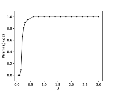
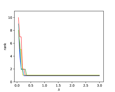
Figure 1: The feature vector $X\sim\mathsf{N}(0,I)$, and the response $Y=f(X)+\epsilon$, where $f(x)=0.1(x_{1}+x_{2}+x_{3})^{3}+\tanh(x_{1}+x_{3}+x_{5})$ and $\epsilon\sim N(0,\sigma^{2})$ with $\sigma=0.1$. Here $n=300$ and $p=50$.
We apply gradient descent to optimize (1.2). For each of $100$ repeated samples of the pair $(X,y)$, we record the solution matrix $\Sigma_{n}^{*}$ across a range of $\lambda$ values from $(0,3]$.
On the left panel, we plot the empirical probability of ${\rm rank}(\Sigma_{n}^{*})\leq 2$ against $\lambda$. On the right panel, we display how the rank of the solution $\Sigma_{n}^{*}$ changes with different $\lambda$ values, using $5$ examples of $(X,y)$. Both plots suggest a remarkable inclination of the solution matrix $\Sigma_{n}^{*}$ towards low-rankness, even though we don’t apply nuclear norm penalties to $\Sigma$ in (1.2) and don’t use early stopping techniques.

In the simulation experiment we collect $n=300$ samples, each having a $50$-dimensional feature vector $X$ from an isotropic normal distribution in $\mathbb{R}^{50}$. The response variable, $Y$, follows a simple relationship with $X$: $Y=0.1(X_{1}+X_{2}+X_{3})^{3}+\tanh(X_{1}+X_{3}+X_{5})+\epsilon$ for some independent noise term $\epsilon\sim\mathsf{N}(0,\sigma^{2})$ with $\sigma=0.1$. Here $(X_{1},X_{2},\ldots,X_{50})$ is the coordinate representation of $X$. Apart from the noise $\epsilon$, $Y$ given $X$ is a combination of two simple functions of linear projections of $X$: cube and hyperbolic tangent.

We apply gradient descent to minimize the kernel learning objective  (1.2) and obtain as output an optimal $50\times 50$ matrix $\Sigma_{n}^{*}$ from the solution tuple $(f_{n}^{*},\gamma_{n}^{*},\Sigma_{n}^{*})$ (further algorithmic details in Section 7). Surprisingly, across repeated trials, this $50\times 50$ matrix $\Sigma_{n}^{*}$ consistently demonstrates a low rank property—${\rm rank}(\Sigma_{n}^{*})\leq 2$—for a wide range of the ridge parameter $\lambda$ (Figure 1). This is intriguing because our experimental design does not include any explicit regularization that promotes low-rankness on the parameter $\Sigma$. For instance, our objective in (1.2) lacks nuclear norm penalties, and our gradient descent algorithm is carefully tuned towards convergence (so no early stopping is used). Yet, the emerging matrix $\Sigma_{n}^{*}$, although noisy, hints at a remarkable low-rank inclination: ${\rm rank}(\Sigma_{n}^{*})\leq 2$, a phenomenon observed across a wide spectrum of $\lambda$ in over 100 repeated experiments.

This low-rank property of the $\Sigma_{n}^{*}$ matrix is neither confined to a specific choice of $X$ distribution nor to a specific choice of functional form for the conditional mean of $Y$ given $X$. We performed a series of experiments of this type and we consistently found this low-rank property in $\Sigma_{n}^{*}$ across a broad spectrum of scenarios. The collection of our experiments and findings will be documented in Section 7.

1.2 Main Results

This paper seeks a quantitative understanding of why the kernel learning objective produces exactly low-rank solutions even in a finite sample setting. We explore

• For what data distribution is the solution, $\Sigma$ of (1.2), expected to be low rank?

• Is this phenomenon observed with different kernels, such as $k_{\Sigma}(x,x^{\prime})=x^{T}\Sigma x^{\prime}$?

To answer these questions, we need to develop a mathematical understanding of the kernel learning objective. For technical reasons, our theoretical findings only apply to a variant of the objective given by

$$\begin{split}\mathop{\rm minimize}_{f,\gamma,\Sigma}~{}~{}~{}\frac{1}{2}\mathbb{E}_{n}\left[(Y-f(X)-\gamma)^{2}\right]+\frac{\lambda}{2}\left\|{f}\right\|_{\mathcal{H}_{\Sigma}}^{2}~{}~{}~{}\mathop{\rm subject\;to}~{}~{}~{}~{}\Sigma\succeq 0,~{}~{}\left|\!\left|\!\left|{\Sigma}\right|\!\right|\!\right|\leq M.\end{split}$$ (1.3)

Here, we introduce a constraint, $\left|\!\left|\!\left|{\Sigma}\right|\!\right|\!\right|\leq M$, where $\left|\!\left|\!\left|{\cdot}\right|\!\right|\!\right|$ represents a unitarily invariant norm on $p$-by-$p$ matrices (e.g., operator norm, Frobenius norm, Schatten norm). The addition of this constraint ensures the existence of a minimizer. Nonetheless, our theoretical findings do not depend on the specific choice of $M$ or the specific norm $\left|\!\left|\!\left|{\cdot}\right|\!\right|\!\right|$ being added.

1.2.1 Data Distribution and Regularity Assumptions

Our main results rely on a few assumptions on the data distributions as well as a mild regularity assumption on the real-valued function $\phi$ in (1.1). Throughout this paper, we assume that the data are independently and identically drawn from $(X,Y)\sim\mathbb{P}$ with $\mathbb{E}[\left\|{X}\right\|_{2}^{4}]<\infty$ and $\mathbb{E}[Y^{2}]<\infty$.

Role of Dimension Reduction

Our first assumption is that a low-dimension linear projection of $X$ captures all information of $Y$ from the conditional mean $\mathbb{E}[Y|X]$. Our hope is, by optimizing $\Sigma$ in the kernel, it learns the projection. Hence, the belief in such a low-dimensional model holds (or approximately holds) is fundamental, and is the main reason why we may hope $\Sigma$ to be low rank.

To formalize this idea, we use dimension reduction concepts from statistics [Coo98]. Specifically, a subspace $S$ is called a mean dimension reduction subspace if $\mathbb{E}[Y|X]=\mathbb{E}[Y|\Pi_{S}X]$, where $\Pi_{S}$ denotes the Euclidean projection onto a subspace $S$ of the ambient space $\mathbb{R}^{p}$. We then introduce the smallest such subspace, termed the central mean subspace in the literature [CL02].

Definition 1.1 (Central Mean Subspace [CL02, Definition 2]).

Let $S_{*}$ denote the intersection over all mean dimension-reduction subspaces:

$$S_{*}=\cap\{S:\mathbb{E}[Y|X]=\mathbb{E}[Y|\Pi_{S}X]\}.$$

If $S_{*}$ itself is a mean dimension-reduction subspace, it is then called the central mean subspace.

Assumption 1 (Existence of Central Mean Subspace).

The central mean subspace $S_{*}$ exists.

Note that the central mean subspace does not always exist, because the intersection of dimension reduction subspaces is not necessarily a dimension reduction subspace. Nonetheless, the central mean subspace does exist under very mild distributional conditions on $X$, e.g., when $X$ is a continuous random variable with convex, open support or has Lebesgue density on $\mathbb{R}^{p}$ [CL02].

Predictive Power

Our second assumption is mild: $X$ has predictive power for $Y$. Interestingly, this seemingly mild assumption is necessary for the phenomenon to occur.

Assumption 2 ($X$ has predictive power of $Y$).

${\rm Var}(\mathbb{E}[Y|X])\neq 0$.

Covariate’s Dependence Structure

Our third assumption is about the dependence structure of the covariate $X$. We’ll denote the orthonormal complement of the subspace $S_{*}$ as $S_{*}^{\perp}$.

Assumption 3 (Dependence Structure of $X$).

(a) ${\rm Cov}(X)$ has full rank, and (b) $\Pi_{S_{*}}X$ is independent of $\Pi_{S_{*}^{\perp}}X$.

Part (a) is mild. Part (b) is stylized. In fact, our extensive numerical experiments suggest the phenomenon holds in many situations where Part (b) is violated. The independence assumption only reflects the limit of what we are able to prove regarding the observed phenomenon. We shall make further comments on this assumption, and make comparisons to existent results in the literature after we state our main theorems (Section 1.5).

Function $\phi$’s Regularity

Finally, our result requires one more regularity condition pertaining to the real-valued function $\phi$ that defines the kernel $k_{\Sigma}$.

Assumption 4 (Regularity of $\phi$).

$\phi(z)=\int e^{-tz}\mu(dt)$ holds for every $z$ where $\mathop{\rm supp}(\mu)\subseteq[m_{\mu},\infty)$ and $m_{\mu}\in(0,\infty)$. Moreover, $\phi_{+}^{\prime}(0)=\lim_{z\to 0^{+}}(\phi(z)-\phi(0))/z$ exists.

The condition draws inspiration from Schoenberg’s fundamental work [Sch38], which characterizes all real-valued functions $\phi$ ensuring $k_{\Sigma}$ is a positive definite kernel for every positive definite matrix $\Sigma$ in every dimension $p$. Such a function $\phi$ must conform to $\phi(z)=\int e^{-tz}\mu(dt)$ with $\mu$ being a finite, nonnegative measure supported on $[0,\infty)$ but not concentrated at zero. The first part of the condition, thereby, can be viewed as a robust requirement of $\mu$ not being a point mass at zero. The second part of the condition implies that $\phi$ is differentiable on $(0,\infty)$, and right differentiable at $0$. So this condition requires $k_{\Sigma}$ to be differentiable. A common kernel that meets these two criteria is the Gaussian kernel.

1.2.2 Formal Statement

Our first result (Theorem 1.1) says that at every one of its population minimizers, the kernel learning objective returns a $\Sigma^{*}$ whose column space is contained in or equal to the central mean subspace $S_{*}$. For clarity, the population objective is given by:

$$\begin{split}\mathop{\rm minimize}_{f,\gamma,\Sigma}~{}~{}~{}\frac{1}{2}\mathbb{E}\left[(Y-f(X)-\gamma)^{2}\right]+\frac{\lambda}{2}\left\|{f}\right\|_{\mathcal{H}_{\Sigma}}^{2}~{}~{}~{}\mathop{\rm subject\;to}~{}~{}~{}~{}\Sigma\succeq 0,~{}~{}\left|\!\left|\!\left|{\Sigma}\right|\!\right|\!\right|\leq M.\end{split}$$ (1.4)

where, instead of taking empirical expectation $\mathbb{E}_{n}$ as seen in equation (1.3), we use expectation $\mathbb{E}$. We’ll use ${\rm col}(\Sigma)$ to denote the column space of a matrix $\Sigma$.

Theorem 1.1.

Let Assumptions 1– 4 hold. Fix a unitarily invariant norm $\left|\!\left|\!\left|{\cdot}\right|\!\right|\!\right|$ and $M\in(0,\infty)$.

Any minimizer $(\Sigma^{*},f^{*},\gamma^{*})$ of the population objective (1.4), obeys the following properties.

• For every $\lambda\in(0,\infty)$, ${\rm col}(\Sigma^{*})\subseteq S_{*}$.

• For every $\lambda\in(0,\lambda_{0}]$ (with some $\lambda_{0}<\infty$ dependent on $M$, $\mathbb{P}$, $\left|\!\left|\!\left|{\cdot}\right|\!\right|\!\right|$), ${\rm col}(\Sigma^{*})=S_{*}$.

Theorem 1.1 is a foundational result for understanding the kernel learning objective. It reveals that the population-level solutions are aligned with the data’s inherent low-dimensional structure. Specifically, when $\lambda$ is sufficiently small, ${\rm col}(\Sigma^{*})=S_{*}$, and ${\rm rank}(\Sigma^{*})=\dim(S_{*})$.

The perhaps surprising result comes when we move from the population to the finite sample kernel learning objective. Our second result, Theorem 1.2, says that in finite samples, the kernel learning objective (with high probability) also delivers a solution $\Sigma_{n}^{*}$ that has rank less than or equal to $\dim(S_{*})$. Remarkably, the low-rank solution is achieved without explicitly incorporating low-rankness promoting regularizers on $\Sigma$ in objective (1.3)!

Theorem 1.2.

Let Assumptions 1– 4 hold. Fix a unitarily invariant norm $\left|\!\left|\!\left|{\cdot}\right|\!\right|\!\right|$ and $M\in(0,\infty)$.

• For every $\lambda\in(0,\infty)$,

  $$\lim_{n\to\infty}\mathbb{P}({\rm rank}(\Sigma_{n}^{*})\leq\dim(S_{*}),~{}~{}\text{$\forall(\Sigma_{n}^{*},f_{n}^{*},\gamma_{n}^{*})~{}\text{minimizing}~{}\eqref{eqn:kernel-learning-objective-variant}$})=1.$$

• For every $\lambda\in(0,\lambda_{0}]$ (with the same $\lambda_{0}<\infty$ in Theorem 1.1):

  $$\lim_{n\to\infty}\mathbb{P}({\rm rank}(\Sigma_{n}^{*})=\dim(S_{*}),~{}~{}\text{$\forall(\Sigma_{n}^{*},f_{n}^{*},\gamma_{n}^{*})~{}\text{minimizing}~{}\eqref{eqn:kernel-learning-objective-variant}$})=1.$$

Theorem 1.2 gives a quantitative formalism of the phenomenon we observe in the data. The subsequent remarks will further explore the implications and nuances of the described phenomenon.

• (A dimension reduction tool) Theorem 1.2 shows that the proposed kernel learning objective can be used for dimension reduction. Corollary 5.1 shows that under the prescribed assumptions 1—4, for $\lambda\in(0,\lambda_{0}]$ where $\lambda_{0}$ is defined in Theorem 1.1, the column space of $\Sigma_{n}^{*}$ converges to $S_{*}$ under the distance measured by the associated projections $\left|\!\left|\!\left|{\Pi_{{\rm col}(\Sigma_{n}^{*})}-\Pi_{S_{*}}}\right|\!\right|\!\right|$.

• (A low-rankness inducing mechanism) Oftentimes, there’s the expectation that explicit regularization techniques, e.g., nuclear norm penalization, early stopping, clipping, etc., are essential to achieve low rank structures in minimization solutions. Theorem 1.2 shows that these are not necessarily needed for the kernel learning objective. In Section 1.3, we delve into the mathematical intuition underpinning Theorem 1.2.

• (Constraint $\Sigma:\Sigma\succeq 0$). Some may contend that the positive semidefinite constraint $\Sigma\succeq 0$, which forces the solution $\Sigma_{n}^{*}$ to have non-negative eigenvalues (akin to eigenvalue thresholding), is serving as the explicit regularization that induces a low rank $\Sigma_{n}^{*}$. Yet our result not only says that $\Sigma_{n}^{*}$ is low-rank but also that its rank is bounded by $\dim(S_{*})$. Note the positive semidefinite constraint alone would not lead to this sharper bound: see the next bullet point.

• (Role of $k_{\Sigma}$). In Section 6 and 7, we examine an alternative kernel objective. Instead of using the kernel as defined in equation (1.1), we consider kernels of the form $(x,x^{\prime})\mapsto\psi(x^{T}\Sigma x^{\prime})$ where $\Sigma$ is positive semidefinite. Empirically, this change results in the absence of the low-rankness phenomenon observed in our earlier simulations.

  Section 1.3 clarifies the role of the kernel $k_{\Sigma}$ defined in equation (1.1), showing how it interacts with our statistical modeling in a way that leads to the phenomenon.

1.3 Technical Insight

This section elucidates our main idea behind proving Theorem 1.2. For space considerations, here we only discuss the case where $\lambda\in(0,\lambda_{0}]$ for the $\lambda_{0}$ defined in Theorem 1.1.

Given Theorem 1.1, any population minimizer $\Sigma^{*}$ must obey ${\rm rank}(\Sigma^{*})=\dim(S_{*})$. Our goal is to show that this low rankness property is preserved by the empirical minimizer $\Sigma_{n}^{*}$:

$$\lim_{n\to\infty}\mathbb{P}({\rm rank}(\Sigma_{n}^{*})=\dim(S_{*}),~{}~{}\text{$\forall(\Sigma_{n}^{*},f_{n}^{*},\gamma_{n}^{*})~{}\text{minimizing}~{}\eqref{eqn:kernel-learning-objective-variant}$})=1.$$

Definitions and Notation

To understand this property of $\Sigma_{n}^{*}$, we first introduce a function that takes partial minimization over the prediction function and the intercept $\gamma$:

$$J_{n}(\Sigma)=\min_{f,\gamma}\frac{1}{2}\mathbb{E}_{n}\left[(Y-f(X)-\gamma)^{2}\right]+\frac{\lambda}{2}\left\|{f}\right\|_{\mathcal{H}_{\Sigma}}^{2}.$$ (1.5)

Then the empirical minimizer $\Sigma_{n}^{*}$ corresponds to a minimizer of

$$\mathop{\rm minimize}_{\Sigma}J_{n}(\Sigma)~{}~{}~{}\text{subject to}~{}~{}~{}\Sigma\succeq 0,~{}\left|\!\left|\!\left|{\Sigma}\right|\!\right|\!\right|\leq M.$$ (1.6)

Similarly, we define the population objective $J(\Sigma)$ by replacing $\mathbb{E}_{n}$ in equation (1.5) by $\mathbb{E}$. Then the population minimizer $\Sigma^{*}$ corresponds to a minimizer of an analogously defined problem:

$$\mathop{\rm minimize}_{\Sigma}J(\Sigma)~{}~{}~{}\text{subject to}~{}~{}~{}\Sigma\succeq 0,~{}\left|\!\left|\!\left|{\Sigma}\right|\!\right|\!\right|\leq M.$$ (1.7)

Let’s define

$$\mathcal{C}=\{\Sigma:\Sigma\succeq 0\}~{}~{}\text{and}~{}~{}\mathcal{M}=\{\Sigma:\Sigma\succeq 0,~{}{\rm rank}(\Sigma)=\dim(S_{*})\}.$$ (1.8)

We use $\mathcal{C}_{M}=\{\Sigma:\Sigma\succeq 0,\left|\!\left|\!\left|{\Sigma}\right|\!\right|\!\right|\leq M\}$ to denote the compact constraint set.

Main Properties

Our strategy relies on establishing two properties of $J$ and $J_{n}$.

• (Sharpness) For every minimizer $\Sigma^{*}$ of the population objective $J$, there is a $\rho>0$ such that

  $$\lim_{t\to 0^{+}}\frac{1}{t}(J(\Sigma^{*}+tW)-J(\Sigma^{*}))\geq\rho\left|\!\left|\!\left|{W}\right|\!\right|\!\right|$$ (1.9)

  holds for every matrix $W$ in the tangent cone of $\mathcal{C}$ at $\Sigma^{*}$ with ${\rm col}(W)\subseteq{\rm col}(\Sigma^{*})^{\perp}$. Additionally, $\nabla J$ exists and is continuous on $\mathcal{C}$ (for gradient definition on $\mathcal{C}$, see Definition 3.1).

  This property emphasizes the stability of $\Sigma^{*}$ as a minimizer: small perturbations in certain directions $W$ lead to an increase in the objective $J$ locally at least linear in the size of $W$. Note the considered perturbations $W$ are those in the tangent cone of $\mathcal{C}$ perpendicular to the set $\mathcal{M}$. Technically, this linear increase of $J$ when deviating away from $\mathcal{M}$ holds not just at $\Sigma^{*}$ but within a neighborhood of $\Sigma^{*}$, thanks to the continuity of $\nabla J$.

  Statistically, given ${\rm col}(\Sigma^{*})=S_{*}$, this property says that perturbation of $\Sigma^{*}$ in any direction $W$ whose columns are orthogonal to the central mean subspace $S_{*}$ would induce such a linear growth of the population objective $J$.

  As a comparison, in classical quadratically mean differentiable models, where the true parameter is statistically identifiable and in the interior of the parameter space, the population objective (expected negative log-likelihood) has a local quadratic growth away from its minimizer (the true model parameter), with the curvature given by the Fisher information [VdV00].

• (Uniform Convergence) The value and gradient of the empirical objective $J_{n}$ converges uniformly in probability to those of the population objective $J$ on the constraint set $\mathcal{C}_{M}$, i.e.,

  $$\begin{split}\sup_{\Sigma\in\mathcal{C}_{M}}|J_{n}(\Sigma)-J(\Sigma)|=o_{P}(1),~{}~{}~{}~{}~{}\sup_{\Sigma\in\mathcal{C}_{M}}\left|\!\left|\!\left|{\nabla J_{n}(\Sigma)-\nabla J(\Sigma)}\right|\!\right|\!\right|=o_{P}(1)\end{split}$$ (1.10)

  as the sample size $n\to\infty$. The $o_{P}(1)$ stands for convergence to zero in probability.

Main Argument

With these properties in mind, our main argument, which is largely inspired by sensitivity analysis of minimizers’ set identifiability in the optimization literature [DL14], is as follows.

• The uniform convergence property of objective values ensures that the empirical minimizers converge (in probability) to their population counterparts as $n\to\infty$. Since all population minimizers fall within $\mathcal{M}$, this implies that the empirical minimizers converge to $\mathcal{M}$.

• To further show the empirical minimizers fall within $\mathcal{M}$, the sharpness property becomes crucial. The sharpness property ensures the empirical objective, whose gradient is uniformly close to that of population objective, is still with high probability sharp, i.e., increasing at least linearly when moving in normal directions away from $\mathcal{M}$ near the population minimizers.

To summarize, while uniform convergence of objective values implies convergence of minimizers, the sharpness property offers the stability that preserves the minimizers’ low rankness property—a special case of set identifiability in optimization—under perturbations.

The role of kernel $k_{\Sigma}$

It’s important to note that the sharpness property (1.9) is fundamentally tied to the kernel defined in (1.1). For kernel objectives that use kernels $(x,x^{\prime})\mapsto\psi(x^{T}\Sigma x^{\prime})$, the low rankness phenomenon does not occur and the objectives do not exhibit the sharpness property.

1.4 Background: Kernel Learning

To place the results in context, we describe its genesis. A large body of research has emphasized the need to consider multiple kernels or parameterization of kernels in regression. The overarching consensus is that choosing the “right” kernel is instrumental for both predictive accuracy and data representation [GA11].

Among many, one prominent method of kernel parameterization is through a linear combination of fixed kernels, represented as $k_{\eta}(x,x^{\prime})=\sum_{i=1}^{M}\eta_{i}k_{i}(x,x^{\prime})$ [LCB⁺04, ZO07]. The aim is to learn the nonnegative weights $\eta$. Several studies show that this approach can enhance predictive performance on real datasets, e.g., [SDBR14, SMCB16]. Nonetheless, the method often falls short in its interpretability. Since the original description of individual features, $x$, is lost during kernel embedding $k_{i}$, it becomes challenging to discern which specific components of our input data, $x$, are the most influential in making predictions.

On the other hand, there’s also a growing interest in learning a scaling parameter $\Sigma$ for kernels, where $k_{\Sigma}(x,x^{\prime})=\phi(\left\|{x-x^{\prime}}\right\|_{\Sigma}^{2})$ as described in (1.1). The primary interests of this approach, as pointed out by several studies, are twofold: the model’s interpretability and its demonstrated effectiveness in predictions across a collection of benchmark real-world datasets.

Among many work that considers learning such a kernel, early work by Vapnik and colleagues [WMC⁺00, CVBM02, GWBV02], for instance, proposed a method equivalent to learning a diagonal matrix $\Sigma$ in $k_{\Sigma}$. This method aids in feature selection by removing redundant coordinates in $x$. Subsequent research by Fukumizu, Bach, and Jordan [FBJ04, FBJ09] pivoted towards learning a projection matrix $\Sigma$ to assist in subspace dimension reduction. Besides enhancing interpretability by removing data redundancy, these models demonstrate good predictive performance in many fields, e.g., bioinformatics [SVV⁺18], and sensing and imaging [SNYB19].

Recent empirical endeavors have consistently explored learning a matrix $\Sigma$ in such a kernel, with numerical findings suggesting that learning such a $\Sigma$ in kernel ridge regressions can outperform random forest, multilayer neural networks and transformers, attaining the state-of-the-art predictive performance in a collection of benchmark datasets [RBPB22].

However, while empirical studies on learning such kernel $k_{\Sigma}$ are abundant, theoretical studies on statistical properties of the solution matrix $\Sigma$ have been relatively scarce. This is the realm where our contribution is mainly focused.

A notable work related to us is the research by Fukumizu, Bach, and Jordan [FBJ09]. Focusing on the problem of sufficient dimension reduction, they studied the statistical properties of empirical minimizer $\Sigma$ within their kernel ridge regression objective. Their main results showed that the column space of $\Sigma$ converges to the target of inference, the central dimension reduction subspace. However, an inherent limitation of their study hinges on a significant assumption: that the dimension $r$ of the central subspace is known. In fact, their algorithm uses this knowledge to enforce an explicit rank constraint $\Sigma\in\Lambda_{r}$ in their kernel objective, where $\Lambda_{r}=\{\Pi_{S}|\dim(S)=r\}$ represents the set of all projection matrices of rank $r$.

In contrast, our research does not require prior knowledge of the dimension of the central mean subspace. We do not place such a rank constraint $\Sigma\in\Lambda_{r}$ in the objective. Our main result shows, under proper statistical modeling assumptions and choice of $\lambda$, the empirical minimizer $\Sigma$ adapts to the problem’s low dimensional structure: ${\rm rank}(\Sigma)=\dim(S_{*})$ simply holds with high probability. We then leverage the result ${\rm rank}(\Sigma)=\dim(S_{*})$ to show the consistency of the column space of $\Sigma$ for the central mean subspace $S_{*}$.

In the most recent development, Jordan and a subset of authors of the current paper delved into a scenario where $\Sigma$ is diagonal [JLR21]. Their findings revolve around projected gradient descent leading to sparse diagonal matrices. However, our focus diverges. We do not dwell on the algorithmic intricacies nor impose diagonal requirements on the matrix $\Sigma$ in our objectives. The proof techniques are also very much different.

1.5 Relation to Dimension Reduction Literature

Theorem 1.2 and Corollary 5.1 demonstrate that our proposed kernel learning procedure can serve as an inferential tool for the central mean subspace. We will now explore its applicability and constraints.

In the context of inference, Assumption 1 is essential. Assumption 2 can be checked statistically using goodness-of-fit test, e.g., [FH01]. Assumption 3, which demands independence between $\Pi_{S_{*}}X$ and $\Pi_{S_{*}^{c}}X$, might seem restrictive. Nonetheless, there are scenarios where our findings are directly applicable, including:

• When we can intentionally design $X$ to follow a specific distribution during data collection, as in computer experiments [SWNW03]. Notably, Assumption 3 is satisfied when $X\sim\mathsf{N}(0,I_{p})$.

• When equipped with prior knowledge regarding the marginal distribution of $X$ [CFJL18]. If $X$ is continuous with support $\mathbb{R}^{p}$, we can then apply the reweighting technique (e.g., [BM87]) to allocate distinct weights to different data points, reducing the inference problem to the case of $X\sim\mathsf{N}(0,I_{p})$. In particular, each data point $X=x$ is given a weight $w(x)=p_{G}(x)/p_{X}(x)$ where $p_{G}$ and $p_{X}$ denote the densities of $\mathsf{N}(0,I_{p})$ and $X$, respectively. In more general cases, the Voronoi weighting method can be utilized to mitigate violations of normality [CN94].

As a comparison, we note that many existent methodologies that target inference of the central mean subspace also hinge on specific distributional assumptions. Notably:

• Sliced Inverse Regression (SIR) [Li91]: The inference method based on sliced inverse regression necessitates a coverage condition, see, e.g., [Coo04, YDS16, LZL18]. This condition doesn’t hold when $Y$ is categorical with values from a set of $k$ elements when $k\leq\dim(S_{*})$ [Coo04].

• Minimum Average Variance Estimation (MAVE) [XTLZ02]: This approach (and related approaches that estimate the derivative of $\mathbb{E}[Y|X=x]$, e.g., [Sam93, HJPS01]) relies on $X$ being continuous and not discrete, see, e.g.,  [XTLZ02, YL11, LLY14].

• Fourier method: This approach assumes Gaussianity of $X$ [ZZ06, Zen08].

• Contour Regression: This method demands that $X$ follow an elliptical distribution [LZC05].

In contrast, our assumptions do not confine $X$ to a specific distribution type or make assumptions about the continuity of $X$ or $Y$. So our assumptions are not more restrictive than existing ones.

Conversely, our assumptions, though not more restrictive, are also not universally more flexible compared to existing ones. When we try to delineate the scenarios and conditions, our assertions aren’t that our assumptions, or procedures, should always be the appropriate ones in practice.

Finally, our procedure infers the central mean subspace without prior knowledge of its dimension (Theorem 1.2 and Corollary 5.1), contrasting with existing kernel dimension reduction methods that rely on a rank constraint assuming prior knowledge of the dimension [FBJ09]. Since this aspect has been elaborated at the near end of Section 1.4, we thereby do not repeat it here.

1.6 Implications for Sparse Regularization

1.6.1 This paper’s Perspective

In statistics and machine learning, regularization often refers to techniques that enforce “simplicity” in solutions. It’s commonly implemented by adding a penalty term to the loss function, thereby deterring solution complexity [HTF09]. To achieve solutions that are “simple” in structure, notable penalty terms such as the $\ell_{1}$ norm encourage vector sparsity, while the nuclear norm targets low-rank matrices [HTW15]. Ideas supporting the importance of penalty terms are based on arguments that sparsity and low rankness of minimizers are inherently unstable under perturbations.

This paper, however, shows that assessing solution sparsity or low rankness based merely on the presence or absence of penalty terms does not capture the full picture. The perspective we offer is grounded in the sensitivity analysis techniques of minimizers’ set identifiability in the optimization literature, e.g., [Wri93, Lew02, HL07, Dru13, DL14, FMP18]. This domain tackles a key problem: given that a solution $\theta^{*}$ to a minimizing objective aligns with the set inclusion $\theta^{*}\in\mathsf{S}$, under what conditions will a smooth perturbation of the objective ensure that the minimizers of the perturbed problems align with the set inclusion $\theta_{n}^{*}\in\mathsf{S}$?

The crux of the answer often lies in the original minimization objective obeying a “sharpness” property around its minimizer (the term “sharpness” is borrowed from, e.g., [Lew02, DL14] among many in the field), which roughly speaking, means that the original objective grows at least linearly when moving away from the set $\mathsf{S}$. Specifically, in nonlinear constrained optimization when $\mathsf{S}$ is a smooth subset of the boundary of a convex constraint set (called an “identifiable surface”), the sharpness property corresponds to the notion of strict complementary slackness at $\theta^{*}$ [Wri93]. When $\mathsf{S}$ is a submanifold of an ambient Euclidean space, this requires the directional derivative of the original objective at $\theta^{*}$ to be bounded away from zero along the normal directions at $\theta^{*}$ with respect to $\mathsf{S}$, which is formally described in the definition of partial smoothness [Lew02]. Defining a “sharpness” condition for a general set $\mathsf{S}$ still relies on case-specific studies (we perform an analysis for a specific set of low-rank matrices for our purpose in Section 5), in which case only the notion of identifiable set captures the broad idea [Dru13, DL14].

Building on this insight, we argue that an empirical minimizer would maintain the “simple” structure of its population solution if the population objective possesses a form of sharpness property in relation to the set of “simple” solutions, and if the gradient and value of the empirical objective converge uniformly to the population counterparts. This perspective is useful as it illuminates why, despite our kernel learning objective lacking explicit nuclear norm regularization (or other low-rank promoting penalties), we still observe an exact low-rank solution in finite samples. Specifically, for our kernel learning objective, the set $\mathsf{S}$ corresponds to the set of low-rank matrices. Since the objective displays a “sharpness” with respect to $\mathsf{S}$, by showing identifiability results with respect to the set of low-rank matrices, we demonstrate the low-rankness of empirical minimizers.

According to this perspective, one aspect of the contribution of this work is to delineate conditions under which the kernel learning objective at the population level displays the desirable sharpness property. Our main theoretical results provide a set of sufficient and necessary conditions for when this happens. We show that Assumption 2 is necessary, and Assumptions 1—3 are sufficient for the kernel defined in (1.1). The sharpness property disappears when the kernel in the objective is replaced by other kernels of the form $(x,x^{\prime})\mapsto\psi(x^{T}\Sigma x^{\prime})$.

1.6.2 Connections to Prior Work on Implicit Regularization

Recent literature demonstrates a collection of methods that induce exact low-rank solutions under the umbrella of implicit regularization. We shall discuss two lines of existent work in which implicit regularization is associated with solutions that are exactly low rank.

The first line of research direction demonstrates that the solution’s low rankness is intimately tied to the algorithm used, e.g., [GWB⁺17, LMZ18, ACHL19, JDST20, LLL21, TVS23]. By contrast, our main result on solutions’ low rankness properties (Theorem 1.2) is algorithm-independent.

Another line of research points out that the solution’s low rankness is intrinsic to the objective, which is related to our current work. A notable example is on the Burer-Monteiro matrix factorization [BM03]. Several studies have shown that minimizing objectives of the following form: (below $L\geq 0$ is a loss function)

$$\mathop{\rm minimize}_{U,V}L(UV^{T})+\frac{\lambda}{2}(\left|\!\left|\!\left|{U}\right|\!\right|\!\right|_{F}^{2}+\left|\!\left|\!\left|{V}\right|\!\right|\!\right|_{F}^{2})$$ (1.11)

yields exact low-rank solutions $UV^{T}$ for large enough $\lambda>0$, despite only involving Frobenius norms or ridge penalties of matrices $U,V$ (see, e.g., [DKS21, TQP22, POW23]). This is due to the equivalence between the matrix factorization objective (1.11) and the nuclear norm penalization:

$$\mathop{\rm minimize}_{\Sigma}L(\Sigma)+\lambda\left|\!\left|\!\left|{\Sigma}\right|\!\right|\!\right|_{{\rm nuc}}$$

utilizing a connection between nuclear and Frobenius norm: $\left|\!\left|\!\left|{\Sigma}\right|\!\right|\!\right|_{{\rm nuc}}=\inf_{\Sigma=UV^{T}}\frac{1}{2}(\left|\!\left|\!\left|{U}\right|\!\right|\!\right|_{F}^{2}+\left|\!\left|\!\left|{V}\right|\!\right|\!\right|_{F}^{2})$ [SRJ04]. This raises the question: can the low-rankness of our kernel learning objective be explained by a known low-rank promoting matrix norm on $\Sigma$?

Before answering this question, it is essential to highlight two fundamental differences between our work and this line of work. First, our modeling of prediction function $f$ accommodates nonlinearity; the low-rankness property of our learning objective vanishes if we model the kernel of $\mathcal{H}_{\Sigma}$ as a linear kernel $(x,x^{\prime})\mapsto x^{T}\Sigma x^{\prime}$. In such a scenario, even though our kernel learning objective might resemble the matrix factorization in Equation (1.11), there are underlying differences. Second, our approach applies a ridge penalty solely to $f$, while permitting arbitrary norm constraints on $\Sigma$. In contrast, the works we refer to predominantly depend on both $U$ and $V$ having Frobenius norms.

Our research contributes a function $J(\Sigma)$ (detailed in Section 1.3), which encourages low-rank solutions under suitable statistical models, which is certainly a first step towards understanding the low rankness phenomenon we observe. However, a comprehensive analysis is needed to ascertain the full extent to which $J(\Sigma)$ influences the low rankness of matrices.

1.7 Basic Definition and Notation

Throughout this paper, we use several standard notation and definitions in the literature.

Notation: We denote the set of real numbers and complex numbers as $\mathbb{R}$ and $\mathbb{C}$, respectively. The complex conjugate of $z\in\mathbb{C}$ is $\bar{z}$. The inner product in $\mathbb{R}^{p}$ is represented as $\langle v_{1},v_{2}\rangle=v_{1}^{T}v_{2}$. $I$ denotes the $p$-by-$p$ identity matrix and ${\rm col}$, $\mathop{\rm tr}$ and $\det$ denote the column space, trace and determinant of a matrix, respectively. ${\rm Sym}_{p}$ denotes the space of $p$-by-$p$ symmetric matrices with inner product $\langle\Sigma_{1},\Sigma_{2}\rangle=\mathop{\rm tr}(\Sigma_{1}^{T}\Sigma_{2})$. A norm $\left|\!\left|\!\left|{\cdot}\right|\!\right|\!\right|$ on $p$-by-$p$ matrices is called a unitarily invariant norm if $\left|\!\left|\!\left|{\Sigma}\right|\!\right|\!\right|=\left|\!\left|\!\left|{O\Sigma(O^{\prime})^{T}}\right|\!\right|\!\right|$ holds for every square matrix $\Sigma$ and orthonormal matrix $O,O^{\prime}$. We write $A\succeq B$ (resp. $A\succ B$) for matrices $A,B\in{\rm Sym}_{p}$ if $A-B$ is positive semidefinite (resp. positive definite). For a differentiable function $f:\mathbb{R}\to\mathbb{R}$, we use $f^{\prime}$ to denote its gradient.

Probability and Measure: The notation $X_{n}=o_{P}(1)$ means that $X_{n}$ converges to zero in probability as $n\to\infty$, and $X_{n}=O_{P}(1)$ means that for every $\epsilon>0$, there exist finite $M,N$ such that $\mathbb{P}(|X_{n}|>M)<\epsilon$ for every $n\geq N$. The $L_{r}$ norm of a random variable $X$ under a probability measure $\mathbb{Q}$ is denoted as $\left\|{X}\right\|_{L_{r}(\mathbb{Q})}$. The support of a nonnegative measure $\mu$ is denoted as $\mathop{\rm supp}(\mu)$.

Convex Analysis: For a convex set $\mathcal{C}$, the tangent cone at $x\in\mathcal{C}$, $\mathcal{T}_{\mathcal{C}}(x)$, is the set of limits $v=\lim_{n\to\infty}t_{n}(x_{n}-x)$ for some sequence $x_{n}\in\mathcal{C}$ and $t_{n}\to\infty$. The normal cone at $x\in\mathcal{C}$, $\mathcal{N}_{\mathcal{C}}(x)$, is the set of $w$ such that $\langle w,v\rangle\leq 0$ for every $v\in\mathcal{T}_{\mathcal{C}}(x)$.

Variational Analysis: Let $f:\mathbb{R}^{p}\mapsto\mathbb{R}\cup\{+\infty\}$ with a point $x\in\mathbb{R}^{p}$ such that $f(x)$ is finite. The subdifferential of $f$ at $x$, denoted by $\partial f(x)$, consists of all vectors $v$ such that $f(\tilde{x})\geq f(x)+\langle v,\tilde{x}-x\rangle+o(\left\|{\tilde{x}-x}\right\|_{2})$ as $\tilde{x}\to x$.

Function Spaces and Norms: The Lebesgue space $\mathcal{L}_{r}(\mathbb{R}^{p})$ consists of $f:\mathbb{R}^{p}\to\mathbb{C}$ such that $\left\|{f}\right\|_{\mathcal{L}_{r}(\mathbb{R}^{p})}<\infty$ where $r\in[1,\infty]$. The space $\mathcal{L}_{2}(\mathbb{R}^{p})$ has inner product $\langle f_{1},f_{2}\rangle_{\mathcal{L}_{2}(\mathbb{R}^{p})}=\int f(x)\overline{g(x)}dx$. The space $\mathcal{C}_{b}(\mathbb{R}^{p})$ consists of all bounded, continuous functions $f:\mathbb{R}^{p}\to\mathbb{C}$ and is endowed with $L_{\infty}$ norm. For ease of notation, we also use $\left\|{f}\right\|_{\infty}$ to represent $\left\|{f}\right\|_{L_{\infty}(\mathbb{R}^{p})}$.

Fourier Transform: $\mathcal{F}f$ denotes the Fourier transform of $f\in\mathcal{L}_{2}(\mathbb{R}^{p})$, where $\mathcal{F}f(\omega)=(2\pi)^{-p}\int e^{-i\langle x,\omega\rangle}f(x)dx$. $\mathcal{F}^{-1}f$ denotes the inverse Fourier transform of $f\in\mathcal{L}_{2}(\mathbb{R}^{p})$: $\mathcal{F}^{-1}f(x)=\int e^{i\langle x,\omega\rangle}f(\omega)d\omega$. The Fourier inversion theorem then asserts that for any $f\in\mathcal{L}_{2}(\mathbb{R}^{p})$, we have $f=\mathcal{F}\mathcal{F}^{-1}f=\mathcal{F}^{-1}\mathcal{F}f$ in $\mathcal{L}_{2}(\mathbb{R}^{p})$.

Kernel: A symmetric function $k:\mathbb{R}^{p}\times\mathbb{R}^{p}\to\mathbb{R}$ is a positive semidefinite kernel if $\sum_{i,j=1}^{m}\alpha_{i}\alpha_{j}k(x_{i},x_{j})\geq 0$ holds for all $m$, $\alpha_{1},\alpha_{2},\ldots,\alpha_{m}\in\mathbb{R}$, and $x_{1},x_{2},\ldots,x_{m}\in\mathbb{R}^{p}$. It is called a positive definite kernel if it is first positive semidefinite, and moreover, $\sum_{i,j=1}^{m}\alpha_{i}\alpha_{j}k(x_{i},x_{j})=0$ holds if and only if $\alpha_{1}=\alpha_{2}=\ldots=\alpha_{m}=0$ for all mutually distinct $x_{1},x_{2},\ldots,x_{m}\in\mathbb{R}^{p}$. It is called an integrally positive definite kernel if $\int_{\mathbb{R}^{p}}\int_{\mathbb{R}^{p}}k(x,x^{\prime})d\nu(x)d\nu(x^{\prime})>0$ holds for every nonzero signed measure $\nu$ on $\mathbb{R}^{p}$ with finite total variation.

1.8 Paper Organization

The rest of the paper is organized as follows.

Section 2 introduces the basic properties of the RKHS $\mathcal{H}_{\Sigma}$.

Section 3 provides the proof of Theorem 1.1, demonstrating that every minimizer of the population objective $J$ is of low rank. Moreover, it formally describes and proves the sharpness property of the population objective $J$ around the population minimizers.

Section 4 establishes that the value and gradient of the empirical objective $J_{n}$ uniformly converge to those of the population objective $J$ on any given compact set.

Section 5 provides the proof of Theorem 1.2, demonstrating that every minimizer of the empirical objective $J_{n}$ is of low rank with high probability. The proof utilizes the results in previous sections.

Section 6 explains why the observed phenomenon does not occur if the kernel in Equation (1.1) is replaced by the inner product kernel $(x,x^{\prime})\mapsto\psi(x^{T}\Sigma x^{\prime})$, as the new population objective no longer satisfies the proper sharpness property.

Section 7 provides additional experiments investigating the scope of the observed phenomenon.

Section 8 concludes the paper with future work discussions.

1.9 Reproducibility

The codes for all experiments and figures are available online:

https://github.com/tinachentc/kernel-learning-in-ridge-regression

2 Preliminaries on the RKHS $\mathcal{H}_{\Sigma}$

This section summarizes the basic properties we need on the kernel $k_{\Sigma}$ and the RKHS $\mathcal{H}_{\Sigma}$.

According to Assumption 4, we are interested in the kernel $k_{\Sigma}$ of the following form.

$$k_{\Sigma}(x,x^{\prime})=\phi(\left\|{x-x^{\prime}}\right\|_{\Sigma}^{2})=\int_{0}^{\infty}e^{-t\left\|{x-x^{\prime}}\right\|_{\Sigma}^{2}}\mu(dt)$$ (2.1)

where $\mu$ is a nonnegative measure whose support is away from zero. This equation expresses the idea that $k_{\Sigma}$ is a weighted sum of the Gaussian kernel $(x,x^{\prime})\mapsto e^{-t\left\|{x-x^{\prime}}\right\|_{\Sigma}^{2}}$ over different scale $t>0$.

For each positive semidefinite kernel $k_{\Sigma}$, there’s an associated RKHS $\mathcal{H}_{\Sigma}$ [Aro50, Wai19]. We shall use $\left\|{\cdot}\right\|_{\mathcal{H}_{\Sigma}}$ and $\langle\cdot,\cdot\rangle_{\mathcal{H}_{\Sigma}}$ to denote the norm and inner product on $\mathcal{H}_{\Sigma}$ throughout this paper. For an introduction to RKHS and its definition, see, e.g.,  [Wai19, Chapter 12].

Our analysis requires four basic properties of the RKHS $\mathcal{H}_{\Sigma}$ whose proofs are relatively standard.

The first concerns embedding of the space $\mathcal{H}_{\Sigma}$ into $\mathcal{C}_{b}(\mathbb{R}^{p})$.

Proposition 1 (Continuous Embedding of $\mathcal{H}_{\Sigma}$ into $\mathcal{C}_{b}(\mathbb{R}^{p})$).

For every $\Sigma\succeq 0$, and $f\in\mathcal{H}_{\Sigma}$:

$$\left\|{f}\right\|_{L_{\infty}(\mathbb{R}^{p})}\leq\sqrt{\phi(0)}\left\|{f}\right\|_{\mathcal{H}_{\Sigma}}.$$

Proof    Fix $f\in\mathcal{H}_{\Sigma}$. For any $x$, $|f(x)|=|\langle f,k_{\Sigma}(x,\cdot)\rangle_{\mathcal{H}_{\Sigma}}|\leq\left\|{f}\right\|_{\mathcal{H}_{\Sigma}}\left\|{k_{\Sigma}(x,\cdot)}\right\|_{\mathcal{H}_{\Sigma}}=\sqrt{\phi(0)}\left\|{f}\right\|_{\mathcal{H}_{\Sigma}}$, where the two identities uses the reproducing property of $k_{\Sigma}$ with respect to $\mathcal{H}_{\Sigma}$. ∎

The second is about the relations between different RKHS $\mathcal{H}_{\Sigma}$ over the matrix parameter $\Sigma\succeq 0$. Let $\mathcal{H}_{I}$ denote the RKHS corresponding to $k_{I}$, which stands for the kernel $k_{I}(x,x^{\prime})=\phi(\left\|{x-x^{\prime}}\right\|_{2}^{2})$ for the identity matrix $I$. We then have the following proposition of $\mathcal{H}_{\Sigma}$.

Proposition 2 (Connections between $\mathcal{H}_{\Sigma}$ and $\mathcal{H}_{I}$).

Let $\Sigma=UU^{T}\succeq 0$ where $\Sigma,U\in\mathbb{R}^{p\times p}$. Then

$$\mathcal{H}_{\Sigma}=\{f:\mathbb{R}^{p}\mapsto\mathbb{R}|\text{there exists $g:\mathbb{R}^{p}\mapsto\mathbb{R}$ such that $f(x)=g(U^{T}x)$ for $g\in\mathcal{H}_{I}$}\}.$$

Moreover, when $\Sigma\succ 0$, we can define a unique mapping $\iota_{U}:\mathcal{H}_{\Sigma}\to\mathcal{H}_{I}$ that maps $f\in\mathcal{H}_{\Sigma}$ to the unique $g\in\mathcal{H}_{I}$ such that $f(x)=g(U^{T}x)$ holds for $x\in\mathbb{R}^{p}$. This mapping $\iota_{U}$ is notably an isometry: $\langle f_{1},f_{2}\rangle_{\mathcal{H}_{\Sigma}}=\langle\iota_{U}f_{1},\iota_{U}f_{2}\rangle_{\mathcal{H}_{I}}$ holds for every $f_{1},f_{2}\in\mathcal{H}_{\Sigma}$.

Proof    This follows from the constructive proof of a general RKHS in [Wai19, Theorem 12.11]. The key observation is that, for $\Sigma=UU^{T}$, the associated kernel $k_{\Sigma}$ obeys $k_{\Sigma}(x,x^{\prime})=k_{I}(U^{T}x,U^{T}x^{\prime})$ for every $x,x^{\prime}$. Note very similar results have also been noticed in the literature, e.g., [FBJ09]. ∎

The third is an explicit characterization of the space $\mathcal{H}_{\Sigma}$. For every positive definite $\Sigma\succ 0$, let us define

$$Q_{\Sigma}(\omega)=\int_{0}^{\infty}\frac{1}{\sqrt{|\det\Sigma|}}\cdot\left(\frac{1}{4\pi t}\right)^{p/2}e^{-\left\|{\omega}\right\|_{(4t\Sigma)^{-1}}^{2}}\mu(dt).$$ (2.2)

Note $Q_{\Sigma}$ is well-defined for every $\Sigma\succ 0$ since $\mu$ has support away from $0$ by Assumption 4.

Proposition 3 (Characterization of the Hilbert Space $\mathcal{H}_{\Sigma}$).

Assume Assumption 4.

Let $\Sigma\succ 0$ be positive definite. The space $\mathcal{H}_{\Sigma}$ consists of functions

$$\mathcal{H}_{\Sigma}=\left\{f\in\mathsf{C}(\mathbb{R}^{p})\cap\mathcal{L}_{2}(\mathbb{R}^{p}):\mathsf{F}f/\sqrt{Q_{\Sigma}}\in\mathcal{L}_{2}(\mathbb{R}^{p})\right\}.$$

The inner product satisfies $\langle f_{1},f_{2}\rangle_{\mathcal{H}_{\Sigma}}=\langle\mathsf{F}f_{1}/\sqrt{Q_{\Sigma}},\mathsf{F}f_{2}/\sqrt{Q_{\Sigma}}\rangle_{\mathcal{L}_{2}(\mathbb{R}^{p})}$ for every $f_{1},f_{2}\in\mathcal{H}_{\Sigma}$.

Proof    Proposition 3 is deduced from the description of a general translation-invariant RKHS, e.g., [Wen04, Theorem 10.12]. The property we use is the following connection between the Fourier transform of $Q_{\Sigma}$ and the kernel $k_{\Sigma}$. First, $k_{\Sigma}(x,x^{\prime})=\Phi_{\Sigma}(x-x^{\prime})$ where $\Phi_{\Sigma}(z)=\phi(\left\|{z}\right\|_{\Sigma}^{2})$. Second, $\mathcal{F}\Phi_{\Sigma}=Q_{\Sigma}$, which equivalently states $\mathcal{F}^{-1}Q_{\Sigma}=\Phi_{\Sigma}$, meaning $\int e^{i\langle\omega,z\rangle}Q_{\Sigma}(\omega)d\omega=\Phi_{\Sigma}(z)$. ∎

The last is about the expressive power of the RKHS $\mathcal{H}_{\Sigma}$. Let us denote

$$\mathcal{H}_{\Sigma}+\mathbb{R}=\left\{u:\mathbb{R}^{p}\to\mathbb{R}\mid u(x)=f(x)+\gamma~{}\text{where}~{}f\in\mathcal{H}_{\Sigma}~{}\text{and}~{}\gamma\in\mathbb{R}\right\}.$$

Proposition 4 (Denseness of $\mathcal{H}_{\Sigma}+\mathbb{R}$ in $\mathcal{L}_{2}(\mathbb{Q})$).

Assume Assumption 4.

Let $\Sigma\succ 0$ be positive definite. For every probability measure $\mathbb{Q}$, $\mathcal{H}_{\Sigma}+\mathbb{R}$ is dense in $\mathcal{L}_{2}(\mathbb{Q})$: given $u\in\mathcal{L}_{2}(\mathbb{Q})$, for any $\epsilon>0$, there exists $u_{\epsilon}\in\mathcal{H}_{\Sigma}+\mathbb{R}$ such that $\left\|{u-u_{\epsilon}}\right\|_{\mathcal{L}_{2}(\mathbb{Q})}<\epsilon$.

Proof    We leverage a result in [FBJ09, Proposition 5], which says, for an RKHS $\mathcal{H}$, $\mathcal{H}+\mathbb{R}$ is dense in $L_{2}(\mathbb{Q})$ for every probability measure $\mathbb{Q}$ if and only if $\mathcal{H}$ is characteristic, meaning that if two probability measures $\mathbb{Q}_{1}$ and $\mathbb{Q}_{2}$ are such that $\int fdQ_{1}=\int fdQ_{2}$ holds for every $f\in\mathcal{H}$, then $\mathbb{Q}_{1}=\mathbb{Q}_{2}$. Using this result, it suffices to show that $\mathcal{H}_{\Sigma}$ is a characteristic RKHS for every $\Sigma\succ 0$.

That $\mathcal{H}_{I}$ being characteristic is implied by a known result on radial kernels [SFL11, Proposition 5], which states that an RKHS with kernel $(x,x^{\prime})\mapsto\int_{0}^{\infty}e^{-t\left\|{x-x^{\prime}}\right\|_{2}^{2}}\nu(dt)$ is characteristic if the finite measure $\nu$ is not a point mass at zero. The case for general $\mathcal{H}_{\Sigma}$ is implied by the fact that $\mathcal{H}_{I}$ is a characteristic RKHS thanks to Proposition 2.

∎

3 Sharpness Property of Population Objective

In this section, we describe a sharpness behavior of the population objective near its minimizer:

$$\mathop{\rm minimize}J(\Sigma)~{}~{}\mathop{\rm subject\;to}~{}\Sigma\succeq 0,~{}\left|\!\left|\!\left|{\Sigma}\right|\!\right|\!\right|\leq M.$$ (3.1)

The first step is to establish a structural property of the minimizer $\Sigma^{*}$ itself, as detailed in Theorem 1.1. Specifically, there exists a constant $\lambda_{0}<\infty$ that depends on $M,\mathbb{P},\left|\!\left|\!\left|{\cdot}\right|\!\right|\!\right|$ such that:

• For every $\lambda>0$, ${\rm col}(\Sigma^{*})\subseteq S_{*}$ holds for every minimizer $\Sigma^{*}$ of (3.1).

• For every $\lambda\in(0,\lambda_{0}]$, ${\rm col}(\Sigma^{*})=S_{*}$ holds for every minimizer $\Sigma^{*}$ of (3.1).

Essentially, this says that the column space of the minimizer $\Sigma^{*}$ for the population objective aligns with the central mean subspace $S_{*}$. We refer to this property as fidelity.

Our second key finding, which we detail in Section 3.2, illustrates that at every minimizer $\Sigma^{*}$, the population objective $J$ exhibits a “sharp” growth, increasing linearly when $\Sigma^{*}$ is perturbed in a direction perpendicular to the central mean subspace $S_{*}$. Specifically, we establish that at every minimizer $\Sigma^{*}$, there is a $\rho>0$ such that for every perturbation $W\in\mathcal{T}_{\mathcal{C}}(\Sigma^{*})$ with ${\rm col}(W)\subseteq S_{*}^{\perp}$:

$$\lim_{t\to 0^{+}}\frac{1}{t}(J(\Sigma^{*}+tW)-J(\Sigma^{*}))\geq\rho\left|\!\left|\!\left|{W}\right|\!\right|\!\right|.$$ (3.2)

We prove the existence of a gradient $\nabla J$ on $\mathcal{C}$ and use it to establish (3.2). We also show that $\nabla J$ is continuous at $\Sigma^{*}$ (with the definition of gradient formally given in Definition 3.1), underscoring the stability of the sharpness property (3.2).

This sharpness property contributes to our main findings regarding kernel learning. It is a key component in guaranteeing that the low-rank structure of the population minimizer, $\Sigma^{*}$, is retained in its empirical counterpart, which we will discuss in Section 5.

Notation

Let us recall that $J(\Sigma)=\min_{f,\gamma}U_{\Sigma}(f,\gamma)$ where

$$U_{\Sigma}(f,\gamma)=\frac{1}{2}\mathbb{E}[(Y-f(X)-\gamma)^{2}]+\frac{\lambda}{2}\left\|{f}\right\|_{\mathcal{H}_{\Sigma}}^{2}.$$

For any matrix $\Sigma$, the tuple $(f_{\Sigma},\gamma_{\Sigma})$ denotes the unique minimizer of $U_{\Sigma}$ (the uniqueness can be proven by standard arguments, see, e.g., [CS02, Proposition 7]), thus $J(\Sigma)=U_{\Sigma}(f_{\Sigma},\gamma_{\Sigma})$. The residual term at $\Sigma$ is denoted as $r_{\Sigma}(x,y)=y-f_{\Sigma}(x)-\gamma_{\Sigma}$.

3.1 Fidelity

This section proves Theorem 1.1.

Let $U\in\mathbb{R}^{p\times p}$ be a possibly asymmetric matrix. We consider the auxiliary function

$$H(U)=\min_{g,\gamma}\frac{1}{2}\mathbb{E}[(Y-g(U^{T}X)-\gamma)^{2}]+\frac{\lambda}{2}\left\|{g}\right\|_{\mathcal{H}_{I}}^{2}.$$ (3.3)

Lemma 3.1.

$J(\Sigma)=H(U)$ holds for every $\Sigma=UU^{T}\succeq 0$.

Proof    For $\Sigma=UU^{T}\succ 0$, that $J(\Sigma)=H(U)$ follows directly from Proposition 2.

For the general case $\Sigma=UU^{T}\succeq 0$, see Appendix C.1. The main idea is, due to representer theorem [SHS01], $J(\Sigma)$ and $H(U)$, as minimum values of kernel ridge regressions, will be equal if the values of kernels at the covariates are the same. Note $k_{\Sigma}(x,x^{\prime})=k_{I}(U^{T}x,U^{T}x^{\prime})$ for all $x,x^{\prime}$. ∎

As a result, any minimizer $\Sigma^{*}$ has the form $\Sigma^{*}=U^{*}(U^{*})^{T}$ where $U^{*}$ minimizes

$$\mathop{\rm minimize}_{U}H(U)~{}~{}~{}\text{subject to}~{}~{}~{}\left|\!\left|\!\left|{UU^{T}}\right|\!\right|\!\right|\leq M.$$ (3.4)

Main Argument

We aim to prove two properties that hold for every minimizer $U^{*}$ of (3.4):

1. For every $\lambda>0$, we have ${\rm col}(U^{*})\subseteq S_{*}$.

2. For every $\lambda\in(0,\lambda_{0}]$, where $\lambda_{0}<\infty$ depends on $M$, $\mathbb{P}$, $\left|\!\left|\!\left|{\cdot}\right|\!\right|\!\right|$, we have ${\rm col}(U^{*})=S_{*}$.

Note $\Sigma^{*}=U^{*}(U^{*})^{T}$ for some minimizer $U^{*}$. Thus ${\rm col}(\Sigma^{*})={\rm col}(U^{*})$ and Theorem 1.1 is implied.

We first prove part (a). Our key observation is the following property of $H$.

Lemma 3.2 (Projection Onto $S_{*}$ Reduces $H$).

For any matrix $U\in\mathbb{R}^{p\times p}$, we have the properties:

1. $H(U)\geq H(\Pi_{S_{*}}U)$.

2. $H(U)>H(\Pi_{S_{*}}U)$ if both $H(U)<H(0)$ and $U\neq\Pi_{S_{*}}U$ hold.

The proof of Lemma 3.2 is deferred to Section 3.1.1.

A short note is $\left|\!\left|\!\left|{\Pi_{S_{*}}UU^{T}\Pi_{S_{*}}}\right|\!\right|\!\right|\leq\left|\!\left|\!\left|{UU^{T}}\right|\!\right|\!\right|$ for any matrix $U$ and unitarily invariant norm $\left|\!\left|\!\left|{\cdot}\right|\!\right|\!\right|$.

Given Lemma 3.2, we prove Part (a). Indeed, we first see that

$$H(U^{*})=J(\Sigma^{*})<J(0)=H(0).$$ (3.5)

In the above, the identities are all based on Lemma (3.1). The inequality is due to Lemma 3.3, whose proof is given in Section 3.1.2.

Lemma 3.3.

Assume Assumption 2. Then the minimum value of (3.1) is strictly less than $J(0)$.

We apply Lemma 3.2[(ii)] to $U^{*}$ and obtain $U^{*}=\Pi_{S_{*}}U^{*}$. This implies ${\rm col}(U^{*})\subseteq S_{*}$.

We now prove Part (b). We first prove that there is $\epsilon_{0}>0$ such that the lower bound holds

$$\inf_{U:{\rm rank}(U)<\dim(S_{*})}H(U)>\mathbb{E}[{\rm Var}(Y|X)]+\epsilon_{0}.$$ (3.6)

To see this, we first note that there’s a pointwise lower bound on $H(U)$ given by:

$$H(U)\geq\mathbb{E}[(Y-\mathbb{E}[Y|U^{T}X])^{2}]=\mathbb{E}[{\rm Var}(Y|\Pi_{{\rm col}(U)}X)].$$

To make this bound uniform over $U$ whose rank is below $\dim(S_{*})$, we take infimum and obtain:

$$\inf_{U:{\rm rank}(U)<\dim(S_{*})}H(U)\geq\inf_{S:\dim(S)<\dim(S_{*})}\mathbb{E}[{\rm Var}(Y|\Pi_{S}X)].$$

Now we will use the fact that $S_{*}$ is the minimal dimension reduction subspace. This definition implies that for any subspace $S$ with $\dim(S)<\dim(S_{*})$, the projection of $X$ onto $S$ does not capture all the information in $X$ about $Y$. Therefore, $\epsilon_{0}(S):=\mathbb{E}[{\rm Var}(Y|\Pi_{S}X)]-\mathbb{E}[{\rm Var}(Y|X)]>0$ holds for any such subspace $S$. Lemma 3.4 further shows that this bound can be made uniform: if we define $\epsilon_{0}:=\inf\{\epsilon_{0}(S):\dim(S)<\dim(S_{*})\}$, then $\epsilon_{0}>0$. The proof is in Appendix C.2.

Lemma 3.4 (Uniform Gap).

$\inf\{\mathbb{E}[{\rm Var}(Y|\Pi_{S}X)]:\dim(S)<\dim(S_{*})\}>\mathbb{E}[{\rm Var}(Y|X)]$.

On the other hand, we will prove that, for the constant $\epsilon_{0}>0$ from (3.6), there exists $\lambda_{0}<\infty$ depending only on $M$, $\mathbb{P}$, and $\left|\!\left|\!\left|{\cdot}\right|\!\right|\!\right|$ such that for every $\lambda\in(0,\lambda_{0}]$:

$$H(U^{*})<\mathbb{E}[{\rm Var}(Y|X)]+\epsilon_{0}$$ (3.7)

To prove this, consider an arbitrary full-rank matrix $U_{0}$ in the feasible set $\{U:\left|\!\left|\!\left|{UU^{T}}\right|\!\right|\!\right|\leq M\}$, and let $\Sigma_{0}=U_{0}U_{0}^{T}\succ 0$. By Proposition 4, the regression function $x\mapsto\mathbb{E}[Y|X=x]\in\mathcal{L}_{2}(\mathbb{P})$ can be arbitrarily well approximated by $\mathcal{H}_{\Sigma_{0}}+\mathbb{R}$ under $\mathcal{L}_{2}(\mathbb{P})$, which implies then $J(\Sigma_{0})<\mathbb{E}[{\rm Var}(Y|X)]+\epsilon_{0}$ for small enough $\lambda$, say $\lambda\in(0,\lambda_{0}]$. Since $H(U_{0})=J(\Sigma_{0})$ by Lemma 3.1, and since $H(U^{*})\leq H(U_{0})$ as $U^{*}$ is the minimizer, the proof is thus complete.

Combining (3.6) and (3.7), we infer that for every $\lambda\in(0,\lambda_{0}]$, any minimizer $U^{*}$ of (3.4) obeys ${\rm rank}(U^{*})\geq\dim(S_{*})$. Since $\Pi_{S_{*}^{\perp}}U^{*}=0$ by Part (a), we get ${\rm rank}(U^{*})=\dim(S_{*})$ and ${\rm col}(U^{*})=S_{*}$.

3.1.1 Proof of Lemma 3.2

In our proof, $\mathbb{E}_{\Pi_{S_{*}^{\perp}}}X$ denotes the marginal expectation with respect to $\Pi_{S_{*}^{\perp}}X$, and $\mathbb{E}[\cdot\mid\Pi_{S_{*}^{\perp}}X]$ represents the conditional expectation (conditioning on $\Pi_{S_{*}^{\perp}}X$). Note $X=\Pi_{S_{*}}X+\Pi_{S_{*}^{\perp}}X$.

Our proof starts with an identity on $H$:

$$\begin{split}2H(U)&=\min_{f,\gamma}\mathbb{E}_{\Pi_{S_{*}^{\perp}}X}\left[\mathbb{E}\big{[}(Y-f(U^{T}\Pi_{S_{*}}X+U^{T}\Pi_{S_{*}^{\perp}}X)-\gamma)^{2}\mid\Pi_{S_{*}^{\perp}}X\big{]}+\lambda\left\|{f}\right\|_{\mathcal{H}_{I}}^{2}\right],\end{split}$$

which satisfies

$$\begin{split}~{}~{}~{}~{}~{}~{}~{}~{}~{}~{}~{}~{}~{}~{}~{}~{}&\geq\mathbb{E}_{\Pi_{S_{*}^{\perp}}X}\left[\min_{f,\gamma}\left\{\mathbb{E}\big{[}(Y-f(U^{T}\Pi_{S_{*}}X+U^{T}\Pi_{S_{*}^{\perp}}X)-\gamma)^{2}\mid\Pi_{S_{*}^{\perp}}X\big{]}+\lambda\left\|{f}\right\|_{\mathcal{H}_{I}}^{2}\right\}\right]\\ &\stackrel{{\scriptstyle(*)}}{{=}}\min_{f,\gamma}\mathbb{E}[(Y-f(U^{T}\Pi_{S_{*}}X)-\gamma)^{2}]+\lambda\left\|{f}\right\|_{\mathcal{H}_{I}}^{2}=2H(\Pi_{S^{*}}U).\end{split}$$ (3.8)

To understand $(*)$, let us introduce

$$\iota(z)=\min_{f,\gamma}V(z;f,\gamma)~{}~{}\text{where}~{}~{}V(z;f,\gamma)=\mathbb{E}[(Y-f(U^{T}\Pi_{S_{*}}X+z)-\gamma)^{2}]+\lambda\left\|{f}\right\|_{\mathcal{H}_{I}}^{2}.$$

A fundamental relation for any function $f$ and scalar $\gamma$ is

$$V(U^{T}\Pi_{S_{*}^{\perp}}X;f,\gamma)=\mathbb{E}\big{[}(Y-f(U^{T}\Pi_{S_{*}}X+U^{T}\Pi_{S_{*}^{\perp}}X)-\gamma)^{2}\mid\Pi_{S_{*}^{\perp}}X\big{]}+\lambda\left\|{f}\right\|_{\mathcal{H}_{I}}^{2}$$

This is because $\mathbb{E}[Y|X]=\mathbb{E}[Y|\Pi_{S_{*}}X]$ and $\Pi_{S_{*}}X$ is independent of $\Pi_{S_{*}^{\perp}}X$ by Assumption 3.

By taking infimum over $f$ and $\gamma$, this leads us to the identity:

$$\iota(U^{T}\Pi_{S_{*}^{\perp}}X)=\min_{f,\gamma}\mathbb{E}\big{[}(Y-f(U^{T}\Pi_{S_{*}}X+U^{T}\Pi_{S_{*}^{\perp}}X)-\gamma)^{2}\mid\Pi_{S_{*}^{\perp}}X\big{]}+\lambda\left\|{f}\right\|_{\mathcal{H}_{I}}^{2}.$$

Furthermore, $z\mapsto\iota(z)$ is a constant due to the translation invariance property of $\mathcal{H}_{I}$: $\left\|{f(\cdot+z)}\right\|_{\mathcal{H}_{I}}=\left\|{f}\right\|_{\mathcal{H}_{I}}$ holds for every $f\in\mathcal{H}_{I}$ and $z\in\mathbb{R}$. Thus, we can deduce $\mathbb{E}_{\Pi_{S_{*}^{\perp}}X}[\iota(U^{T}\Pi_{S_{*}^{\perp}}X)]=\iota(0)$, validating $(*)$ in our earlier identity.

At this point, we have proven for every matrix $U$:

$$H(U)\geq H(\Pi_{S^{*}}U).$$

Now we investigate the equality case $H(U)=H(\Pi_{S_{*}}U)$.

The inequality in (3.8) becomes an equality if and only if

$$f_{0}(x+c)=f_{0}(x)~{}~{}\text{holds for every $c\in\mathop{\rm supp}(U^{T}\Pi_{S_{*}^{\perp}}X)$}$$

where $(f_{0},\gamma_{0})=\mathop{\rm argmin}_{f,\gamma}\mathbb{E}[(Y-f(U^{T}\Pi_{S_{*}}X)-\gamma)^{2}]+\lambda\left\|{f}\right\|_{\mathcal{H}_{I}}^{2}$.

Below we consider the case where $U\neq\Pi_{S_{*}}U$, or equivalently, $\Pi_{S_{*}^{\perp}}U\neq 0$.

By Assumption 3, ${\rm Cov}(X)$ is full rank, thus implying that $f_{0}(\cdot+c)=f_{0}(\cdot)$ for some $c\neq 0$. Taking the Fourier transform yields $\mathcal{F}f_{0}(\omega)e^{i\langle c,\omega\rangle}=\mathcal{F}f_{0}(\omega)$ for almost everywhere $\omega$ in $\mathbb{R}^{p}$, and since $c\neq 0$, $\mathcal{F}f_{0}(\omega)=0$ holds almost everywhere $\omega$ in $\mathbb{R}^{p}$ under the Lebesgue measure. As $f_{0}\in\mathcal{H}_{I}$ is continuous on $\mathbb{R}^{p}$, this implies that $f_{0}(x)=0$ for all $x$, which only occurs when $H(U)=H(0)=\frac{1}{2}{\rm Var}(Y)$.

Thus, if $H(U)<H(0)$ and $U\neq\Pi_{S_{*}}U$, then $H(U)>H(\Pi_{S^{*}}U)$. This completes the proof.

3.1.2 Proof of Lemma 3.3

It suffices to prove that $J(\Sigma)<J(0)$ for any full rank matrix $\Sigma$ in the feasible set $\{\Sigma:\left|\!\left|\!\left|{\Sigma}\right|\!\right|\!\right|\leq M\}$. For a matrix $\Sigma$, recall our notation $J(\Sigma)=\min_{f,\gamma}U_{\Sigma}(f,\gamma)$, where $U_{\Sigma}(f,\gamma)$ denotes

$$U_{\Sigma}(f,\gamma)=\frac{1}{2}\mathbb{E}[(Y-f(X)-\gamma)^{2}]+\frac{\lambda}{2}\left\|{f}\right\|_{\mathcal{H}_{\Sigma}}^{2}.$$

Also, recall that $(f_{\Sigma},\gamma_{\Sigma})$ is the (unique) minimizer of the functional $(f,\gamma)\mapsto U_{\Sigma}(f,\gamma)$. A basic characterization of $f_{\Sigma}$ is through the Euler-Lagrange equation associated with $\min_{f,\gamma}U_{\Sigma}(f,\gamma)$.

Lemma 3.5 (Euler-Lagrange).

Fix $\Sigma\succeq 0$. The identity below holds for every $h\in\mathcal{H}_{\Sigma}$:

$$\mathbb{E}[r_{\Sigma}(X,Y)h(X)]=\lambda\langle f_{\Sigma},h\rangle_{\mathcal{H}_{\Sigma}}.$$ (3.9)

Proof    This follows by taking the first variation of the cost function $U_{\Sigma}(f,\gamma)$ w.r.t. $f$. ∎

Let’s go back to the proof of Lemma 3.3.

First, $J(0)=\frac{1}{2}{\rm Var}(Y)$ where the minimizer is $f_{0}\equiv 0$ and $\gamma_{0}=0$.

Next, we show $J(\Sigma)<\frac{1}{2}{\rm Var}(Y)$ for any full rank $\Sigma$. It suffices to show that $(f_{\Sigma},\gamma_{\Sigma})\neq(f_{0},\gamma_{0})$, which would then imply $J(\Sigma)=U_{\Sigma}(f_{\Sigma},\gamma_{\Sigma})<U_{\Sigma}(f_{0},\gamma_{0})=\frac{1}{2}{\rm Var}(Y)$.

Now, suppose on the contrary that $f_{\Sigma}\equiv 0$ and $\gamma_{\Sigma}=\mathbb{E}[Y]$. Then (3.9) implies ${\rm Cov}(Y,h(X))=0$ for every $h\in\mathcal{H}_{\Sigma}$. Equivalently, $\mathbb{E}[(\mathbb{E}[Y|X]-\mathbb{E}[Y])(h(X)+\gamma)]=0$ for every $h\in\mathcal{H}_{\Sigma},\gamma\in\mathbb{R}$. By Proposition 4, the function $x\mapsto\mathbb{E}[Y|X=x]-\mathbb{E}[Y]$ can be approximated arbitrarily well by the set $\mathcal{H}_{\Sigma}+\mathbb{R}$ under $\mathcal{L}_{2}(\mathbb{P})$. This then implies that $\mathbb{E}[Y|X]-\mathbb{E}[Y]=0$ holds almost surely under $\mathbb{P}$, indicating ${\rm Var}(\mathbb{E}[Y|X])=0$ which contradicts Assumption 2!

As a result, $(f_{\Sigma},\gamma_{\Sigma})\neq(f_{0},\gamma_{0})$ and $J(\Sigma)<J(0)$ for every full rank $\Sigma$.

3.2 Sharpness

We now prove that at every minimizer, the sharpness property (i.e., (3.2)) holds.

We start by analyzing the differentiability property of the function $J:\mathcal{C}\to\mathbb{R}$. To deal with matrices $\Sigma$ that lie on the boundaries of $\mathcal{C}$, we introduce the following notion of gradient.

Definition 3.1 (Gradient Notion on $\mathcal{C}$).

Let $f:\mathcal{C}\to\mathbb{R}$. The function $f$ has a gradient $\nabla f(\Sigma)$ at $\Sigma\in\mathcal{C}$ if $\nabla f(\Sigma)$ is a symmetric matrix, and for every converging sequence $\Sigma_{n}\in\mathcal{C}$ to $\Sigma$:

$$f(\Sigma_{n})=f(\Sigma)+\langle\nabla f(\Sigma),\Sigma_{n}-\Sigma\rangle+o(\left\|{\Sigma_{n}-\Sigma}\right\|_{F}).$$

We say $f$ is differentiable on $\mathcal{C}$ if $\nabla f$ is everywhere well-defined on $\mathcal{C}$.

Remark     The gradient of $f$ at $\Sigma$, if exists, is unique due to the tangent cone $\mathcal{T}_{\mathcal{C}}(\Sigma)$ containing an open ball. It coincides with the standard notion of gradient for every $\Sigma$ in the interior of $\mathcal{C}$.

The following lemma shows that $J$ is differentiable on $\mathcal{C}$. The crux of Lemma 3.6 is the explicit gradient formula provided in equation (3.10).

Lemma 3.6 (Gradient Formula).

The gradient $\nabla J(\Sigma)$ exists at every $\Sigma\in\mathcal{C}$ with

$$\nabla J(\Sigma)=-\frac{1}{2\lambda}\mathbb{E}[r_{\Sigma}(X,Y)r_{\Sigma}(X^{\prime},Y^{\prime})\partial_{\Sigma}k_{\Sigma}(X,X^{\prime})].$$ (3.10)

In the above, $(X^{\prime},Y^{\prime})$ stands for an independent copy of $(X,Y)$. Also, $\nabla J$ is continuous on $\mathcal{C}$.

The intuition of the gradient formula (3.10) is discussed in Section 3.3. The proof details can be found in Appendix B.

We now establish a form of non-degeneracy condition at every minimizer $\Sigma^{*}$ in Theorem 3.1. The non-degeneracy condition (3.11) is indeed equivalent to the sharpness property of the objective at $\Sigma^{*}$ presented in Corollary 3.1, and also, bears a close resemblance to the notion of strict complementary slackness condition at $\Sigma^{*}$ from the optimization literature (see Remark after Corollary 3.1).

Theorem 3.1 (Non-degeneracy Condition at $\Sigma^{*}$).

Let Assumptions 1–4 hold. Fix $M\in(0,\infty),\left|\!\left|\!\left|{\cdot}\right|\!\right|\!\right|$.

Let $\lambda\in(0,\infty)$. For any minimizer $\Sigma^{*}$ of (3.1), there exists $\rho>0$ such that the following holds:

$$\Pi_{S_{*}^{\perp}}\nabla J(\Sigma^{*})\Pi_{S_{*}^{\perp}}\succeq\rho\Pi_{S_{*}^{\perp}}.$$ (3.11)

Proof    We verify the condition (3.11).

Recall $\phi(z)=\int_{0}^{\infty}\exp(-tz)\mu(dt)$. Let us introduce $\tilde{\phi}(z)=\int_{0}^{\infty}\exp(-tz)\tilde{\mu}(dt)$ where $\tilde{\mu}(dt)=t\mu(dt)$. Note that under Assumption 4, we can express the gradient $\partial_{\Sigma}k_{\Sigma}(x,x^{\prime})$ as the following matrix:

$$\partial_{\Sigma}k_{\Sigma}(x,x^{\prime})=-\tilde{k}_{\Sigma}(x,x^{\prime})\cdot(x-x^{\prime})(x-x^{\prime})^{T}.$$

where $\tilde{k}_{\Sigma}(x,x^{\prime})=\tilde{\phi}(\left\|{x-x^{\prime}}\right\|_{\Sigma}^{2})$. Substituting this formula into Eq. (3.10) results in

$$\nabla J(\Sigma)=\frac{1}{2\lambda}\mathbb{E}\left[r_{\Sigma}(X,Y)r_{\Sigma}(X^{\prime},Y^{\prime})\tilde{k}_{\Sigma}(X,X^{\prime})\cdot(X-X^{\prime})(X-X^{\prime})^{T}\right].$$ (3.12)

Let $\Sigma^{*}$ denote a minimizer of $J$. Recall Theorem 1.1 states that ${\rm col}(\Sigma^{*})\subseteq S_{*}$. Consequentially, using equation (3.12), we obtain the following identity at $\Sigma=\Sigma^{*}$:

$$\begin{split}\Pi_{S_{*}^{\perp}}\nabla J(\Sigma^{*})\Pi_{S_{*}^{\perp}}&=\frac{1}{2\lambda}\mathbb{E}\left[r_{\Sigma^{*}}(X,Y)r_{\Sigma^{*}}(X^{\prime},Y^{\prime})\tilde{k}_{\Sigma}(X,X^{\prime})\cdot\Pi_{S_{*}^{\perp}}(X-X^{\prime})(X-X^{\prime})^{T}\Pi_{S_{*}^{\perp}}\right]\\ &=\frac{1}{2\lambda}\mathbb{E}[r_{\Sigma^{*}}(X,Y)r_{\Sigma^{*}}(X^{\prime},Y^{\prime})\tilde{k}_{\Sigma^{*}}(X,X^{\prime})]\cdot\mathbb{E}[\Pi_{S_{*}^{\perp}}(X-X^{\prime})(X-X^{\prime})^{T}\Pi_{S_{*}^{\perp}}].\end{split}$$ (3.13)

The last line is due to the following. The term $\Pi_{S_{*}^{\perp}}(X-X^{\prime})(X-X^{\prime})^{T}\Pi_{S_{*}^{\perp}}$ is a function of $\Pi_{S_{*}^{\perp}}X$ and $\Pi_{S_{*}^{\perp}}X^{\prime}$. On the other hand, $\tilde{k}_{\Sigma^{*}}(X,X^{\prime})$ is a function of $\Pi_{S^{*}}X$ and $\Pi_{S^{*}}X^{\prime}$ since ${\rm col}(\Sigma^{*})\subseteq S_{*}$. Additionally, $\mathbb{E}[r_{\Sigma^{*}}(X,Y)|X]=\mathbb{E}[r_{\Sigma^{*}}(X,Y)|\Pi_{S_{*}}X]$ by the definition of $S_{*}$ and by Proposition 2. Because $\Pi_{S_{*}}X$ and $\Pi_{S_{*}^{\perp}}X$ are independent by Assumption 3, it then implies that the two terms

$$\mathbb{E}[r_{\Sigma^{*}}(X,Y)r_{\Sigma^{*}}(X^{\prime},Y^{\prime})\tilde{k}_{\Sigma^{*}}(X,X^{\prime})|X,X^{\prime}]~{}~{}\text{and}~{}~{}\Pi_{S_{*}^{\perp}}(X-X^{\prime})(X-X^{\prime})^{T}\Pi_{S_{*}^{\perp}}$$

are also independent. This allows us to split the expectation of their product into the product of their expectations, resulting in the last line of (3.13).

To complete the proof of Theorem 3.1, we further lower bound the RHS of Eq. (3.13).

First, for $\gamma$ defined to be the minimum eigenvalue of ${\rm Cov}(X)$, with $\gamma>0$ by Assumption 3, we have the lower bound:

$$\mathbb{E}[\Pi_{S_{*}^{\perp}}(X-X^{\prime})(X-X^{\prime})^{T}\Pi_{S_{*}^{\perp}}]\succeq\gamma\Pi_{S_{*}^{\perp}}.$$ (3.14)

Next, we show the quadratic form satisfies

$$\mathbb{E}[r_{\Sigma^{*}}(X,Y)r_{\Sigma^{*}}(X^{\prime},Y^{\prime})\tilde{k}_{\Sigma^{*}}(X,X^{\prime})]>0.$$ (3.15)

To prove it, a key observation is that the mapping $(x,x^{\prime})\mapsto\tilde{k}_{I}(x,x^{\prime})$ is an integrally positive definite kernel, which means that for any nonzero signed measure $\nu$ with finite total variation, $\int_{\mathbb{R}^{p}}\int_{\mathbb{R}^{p}}\tilde{k}_{I}(x,x^{\prime})\nu(dx)\nu(dx^{\prime})>0$. This property can be deduced by Proposition 5 of [SFL11], given the fact that $\tilde{k}_{I}$ is a radial kernel with $\tilde{\mu}$ not a zero measure. For a more transparent argument, we introduce the notation $\zeta_{t}(\omega)=\frac{1}{(4\pi t)^{p/2}}e^{-\left\|{\omega}\right\|_{2}^{2}/(4t)}$ and note the following calculations:

$$\begin{split}\iint\tilde{k}_{I}(x,x^{\prime})\nu(dx)\nu(dx^{\prime})&\stackrel{{\scriptstyle(a)}}{{=}}\iint\left(\int e^{-t\left\|{x-x^{\prime}}\right\|_{2}^{2}}\tilde{\mu}(dt)\right)\nu(dx)\nu(dx^{\prime})\\ &\stackrel{{\scriptstyle(b)}}{{=}}\iint\left(\iint e^{-i\langle x-x^{\prime},\omega\rangle}\zeta_{t}(\omega)d\omega\tilde{\mu}(dt)\right)\nu(dx)\nu(dx^{\prime})\\ &\stackrel{{\scriptstyle(c)}}{{=}}\iint\left(\iint e^{-i\langle x-x^{\prime},\omega\rangle}\nu(dx)\nu(dx^{\prime})\right)\zeta_{t}(\omega)d\omega\tilde{\mu}(dt)\\ &=\iint\left|\int e^{-i\langle x,\omega\rangle}\nu(dx)\right|^{2}\zeta_{t}(\omega)d\omega\tilde{\mu}(dt).\end{split}$$ (3.16)

In the above, step $(a)$ is due to the definition of $\tilde{k}_{I}$, step $(b)$ is due to the known fact that Fourier transform of Gaussian is Gaussian and step $(c)$ is due to Fubini’s theorem. Given $\zeta_{t}(\omega)>0$ for all $t,\omega$, the integral in the final expression is nonnegative, and since $\tilde{\mu}$ is not a zero measure, the integral is zero only if $\omega\mapsto\int e^{-i\langle x,\omega\rangle}\nu(dx)$ is a zero constant, which happens only when $\nu$ is a zero measure. This proves that $\iint\tilde{k}_{I}(x,x^{\prime})\nu(dx)\nu(dx^{\prime})>0$ for all nonzero finite signed measure $\nu$.

Next, write $\Sigma^{*}=(U^{*})(U^{*})^{T}$. It is important to note that $\mathbb{E}[r_{\Sigma^{*}}(X,Y)|X]=\mathbb{E}[r_{\Sigma^{*}}(X,Y)|\Pi_{S_{*}}X]$ by the definition of $S_{*}$ and by Proposition 2, and thus $\mathbb{E}[r_{\Sigma^{*}}(X,Y)|X]$ is just a function of $(U^{*})^{T}X$. Let’s write $\mathbb{E}[r_{\Sigma^{*}}(X,Y)|X]=\tilde{r}_{\Sigma^{*}}(Z)$ for some function $\tilde{r}_{\Sigma^{*}}$ where $Z=(U^{*})^{T}X$. With this notation, we can rewrite (3.15) to be $\mathbb{E}[\tilde{r}_{\Sigma^{*}}(Z)\tilde{r}_{\Sigma^{*}}(Z^{\prime})\tilde{k}_{I}(Z,Z^{\prime})]>0$. Given we showed that $(x,x^{\prime})\mapsto\tilde{k}_{I}(x,x^{\prime})$ is integrally positive definite, it is sufficient to show that $\tilde{r}_{\Sigma^{*}}(Z)$ is not almost surely equal to zero, or equivalently, $\mathbb{E}[r_{\Sigma^{*}}(X,Y)|X]$ is not almost surely equal to zero under the probability measure $\mathbb{P}$.

To see the last part $\mathbb{E}[r_{\Sigma^{*}}(X,Y)|X]\neq 0$, we use the Euler-Lagrange equation. Note the Euler-Lagrange equation (Lemma 3.5) shows the following holds for every $h\in\mathcal{H}_{\Sigma^{*}}$:

$$\mathbb{E}[r_{\Sigma^{*}}(X,Y)h(X)]=\lambda\langle f_{\Sigma^{*}},h\rangle_{\mathcal{H}_{\Sigma}^{*}}.$$ (3.17)

Suppose $\mathbb{E}[r_{\Sigma^{*}}(X,Y)|X]=0$. Then $f_{\Sigma^{*}}=0$ must be the zero function. Then $r_{\Sigma^{*}}(X,Y)=Y-\mathbb{E}[Y]$ which in turn implies $\mathbb{E}[Y|X]=\mathbb{E}[Y]$ and ${\rm Var}(\mathbb{E}[Y|X])=0$, a contradiction to Assumption 2. This means that $\mathbb{E}[r_{\Sigma^{*}}(X,Y)|X]\neq 0$ under the $\mathcal{L}_{2}(\mathbb{P})$, and thereby the inequality (3.15) holds.

Finally, based on (3.13), (3.14), and (3.15), we can immediately see the existence of $\rho>0$ such that the nondegeneracy condition (3.11) holds.

∎

Corollary 3.1 (Sharpness Property).

Let Assumptions 1–4 hold. Fix $M\in(0,\infty)$ and $\left|\!\left|\!\left|{\cdot}\right|\!\right|\!\right|$.

Let $\lambda\in(0,\infty)$. For any minimizer $\Sigma^{*}$, there exists $\rho>0$ such that

$$\langle\nabla J(\Sigma^{*}),W\rangle\geq\rho\left|\!\left|\!\left|{W}\right|\!\right|\!\right|$$ (3.18)

holds for every matrix $W\in\mathcal{T}_{\mathcal{C}}(\Sigma^{*})$ with ${\rm col}(W)\subseteq S_{*}^{\perp}$.

Proof    The proof uses a basic characterization of the set

$$\mathcal{W}=\{W:W\in\mathcal{T}_{\mathcal{C}}(\Sigma^{*}),~{}{\rm col}(W)\subseteq S_{*}^{\perp}\}.$$

Lemma 3.7.

$\mathcal{W}=\{W:W=\Pi_{S_{*}^{\perp}}W\Pi_{S_{*}^{\perp}}\succeq 0\}$.

Proof    Suppose $W\in\mathcal{W}$. Now we argue that $W=\Pi_{S_{*}^{\perp}}W\Pi_{S_{*}^{\perp}}\succeq 0$.

To see this, we first note that $W\in\mathcal{T}_{\mathcal{C}}(\Sigma^{*})$. This implies that $W=\lim_{n}t_{n}(\Sigma_{n}-\Sigma^{*})$ for some sequence $\Sigma_{n}\in\mathcal{C}$ and $t_{n}>0$. As ${\rm col}(\Sigma^{*})\subseteq{\rm col}(S_{*})$ by Theorem 1.1, this shows $\Pi_{S_{*}^{\perp}}(\Sigma_{n}-\Sigma^{*})\Pi_{S_{*}^{\perp}}=\Pi_{S_{*}^{\perp}}\Sigma_{n}\Pi_{S_{*}^{\perp}}\succeq 0$ for every $n$. As a result, $\Pi_{S_{*}^{\perp}}W\Pi_{S_{*}^{\perp}}=\lim_{n}\{t_{n}\Pi_{S_{*}^{\perp}}(\Sigma_{n}-\Sigma^{*})\Pi_{S_{*}^{\perp}}\}\succeq 0$. Because we have further $W=W^{T}$ and ${\rm col}(W)\subseteq S_{*}^{\perp}$, this yields $W=\Pi_{S_{*}^{\perp}}W\Pi_{S_{*}^{\perp}}\succeq 0$.

On the other hand, it is clear that any matrix $W\succeq 0$ must belong to $\mathcal{T}_{\mathcal{C}}(\Sigma^{*})$, and any matrix $W=\Pi_{S_{*}^{\perp}}W\Pi_{S_{*}^{\perp}}$ must obey ${\rm col}(W)\subseteq S_{*}^{\perp}$. ∎

Take $W\in\mathcal{T}_{\mathcal{C}}(\Sigma^{*})$ with ${\rm col}(W)\subseteq{\rm col}(S_{*}^{\perp})$. Then $W=\Pi_{S_{*}^{\perp}}W\Pi_{S_{*}^{\perp}}\succeq 0$ by Lemma 3.7. Thereby,

$$\langle\nabla J(\Sigma^{*}),W\rangle=\langle\Pi_{S_{*}^{\perp}}\nabla J(\Sigma^{*})\Pi_{S_{*}^{\perp}},W\rangle.$$

Note we can lower bound the RHS quantity by $\rho\mathop{\rm tr}(W)$ for any constant $\rho>0$ that satisfies the non-degeneracy condition (3.11) in Theorem 3.1. The proof is complete since the mappings $W\mapsto\mathop{\rm tr}(W)$ and $W\mapsto\left|\!\left|\!\left|{W}\right|\!\right|\!\right|$ are uniformly bounded by each other up to a positive constant over $W\in\mathcal{C}$. ∎

Remark    (Equivalence between sharpness property and non-degeneracy condition)

From the proof of Corollary 3.1, we can see the non-degeneracy condition (3.11) and the sharpness property (3.18) are indeed equivalents. Specifically, given $\Sigma$ for which ${\rm col}(\Sigma)\subseteq S$ where $S$ is a linear subspace:

A differentiable function $f:\mathcal{C}\to\mathbb{R}$ is said to satisfy the non-degeneracy condition at $\Sigma\in\mathcal{C}$ if $\Pi_{S^{\perp}}\nabla J(\Sigma)\Pi_{S^{\perp}}\succeq\rho\Pi_{S^{\perp}}$ for some $\rho>0$. This is equivalent to the sharpness property that requires for some $\rho>0$, $\langle\nabla f(\Sigma),W\rangle\geq\rho\left|\!\left|\!\left|{W}\right|\!\right|\!\right|$ holds for all $W\in\mathcal{T}_{\mathcal{C}}(\Sigma)$ with ${\rm col}(W)\subseteq S^{\perp}$.

Remark    (Connection between non-degeneracy condition and strict complementary slackness)

The non-degeneracy condition (3.11) at the minimizer $\Sigma^{*}$ bears a close resemblance, albeit distinct from, the strict complementary slackness condition in optimization [Ber97, Sectioni 3.3.3].

Below we discuss their connections. Suppose $\left|\!\left|\!\left|{\Sigma^{*}}\right|\!\right|\!\right|<M$ holds. Then $\Sigma^{*}$ is a local minimizer of

$$\mathop{\rm minimize}_{\Sigma}J(\Sigma)~{}~{}~{}\mathop{\rm subject\;to}~{}~{}~{}\Sigma\succeq 0.$$

where $\Sigma\succeq 0$ is the only possibly active constraint for the minimizer $\Sigma^{*}$. The strict complementary slackness condition at $\Sigma^{*}$ is then as follows: for some constant $\rho>0$,

$$\Pi_{{{\rm col}(\Sigma^{*})}^{\perp}}\nabla J(\Sigma^{*})\Pi_{{{\rm col}(\Sigma^{*})}^{\perp}}\succeq\rho\Pi_{{{\rm col}(\Sigma^{*})}^{\perp}}.$$ (3.19)

Clearly, the non-degeneracy condition (3.11) and the complementary slackness condition (3.19) are identical when ${\rm col}(\Sigma^{*})=S_{*}$, which occurs when $\lambda\in(0,\lambda_{0}]$ by Theorem 1.1. In such situations, we’ll demonstrate that the empirical minimizer $\Sigma_{n}^{*}$ retains the same rank, $\dim(S_{*})$, as the population minimizer $\Sigma^{*}$ with high probability.

However, for general $\lambda>0$, the most we can say is that ${\rm col}(\Sigma^{*})\subseteq S_{*}$ as also indicated by Theorem 1.1. Given this, the non-degeneracy condition (3.11) is implied by the strict complementary slackness condition (3.19), but not the other way around. In this more general setting, we’ll show the empirical minimizer $\Sigma_{n}^{*}$ has rank at most $\dim(S_{*})$ with high probability.

3.3 Discussion of Gradient Formula

The gradient formula (3.10) expresses a relation between the gradient of the objective $J$ and the residual $r$, both implicitly defined through the variational problem (1.4).

In this section, we describe a brief set of heuristics that render this formula plausible. For simplicity, we first restrict our discussion to $\Sigma\succ 0$. Formal justifications of the gradient formula (3.10) based on the intuitions below for all $\Sigma\succeq 0$ are given in Appendix B.

3.3.1 Invoking the Envelope Theorem

Recall that $J$ is the minimum value of the variational problem.

$$J(\Sigma)=\min_{f,\gamma}\frac{1}{2}\mathbb{E}[(Y-f(X)-\gamma)^{2}]+\frac{\lambda}{2}\left\|{f}\right\|_{\mathcal{H}_{\Sigma}}^{2}.$$ (3.20)

Let us use $(f_{\Sigma},\gamma_{\Sigma})$ to denote the minimizer of the variational problem on the RHS.

Our derivation starts with an application of the envelope theorem, which states under regularity conditions, the gradient of the value function of a variational problem $v(x)=\min_{y}c(x,y)$ exists, and satisfies $\nabla v(x)=\partial_{x}c(x,y(x))$ where $y(x)$ is the minimizer of $\min_{y}c(x,y)$ for a given $x$.

We wish to apply the envelope theorem to obtain a formula for the gradient of $J$. We substitute the analytic form of $\left\|{f}\right\|_{\mathcal{H}_{\Sigma}}$ into equation (3.20):

$$J(\Sigma)=\min_{f,\gamma}\frac{1}{2}\mathbb{E}[(Y-f(X)-\gamma)^{2}]+\frac{\lambda}{2}\int\frac{|\mathsf{F}f(\omega)|^{2}}{Q_{\Sigma}(\omega)}d\omega.$$ (3.21)

Assume regularity holds so the envelope theorem applies. Then we are able to derive

$$\nabla J(\Sigma)=-\frac{\lambda}{2}\int\frac{|\mathsf{F}f_{\Sigma}(\omega)|^{2}}{Q^{2}_{\Sigma}(\omega)}\partial_{\Sigma}Q_{\Sigma}(\omega)d\omega.$$ (3.22)

Operationally, we derive equation (3.22) following the envelope theorem. Indeed, we start by taking the partial derivative of the cost function of the variational problem (3.21) with respect to $\Sigma$, and then replace $f$ with $f_{\Sigma}$ since $(f_{\Sigma},\gamma_{\Sigma})$ is the minimizer of the variational problem for a given $\Sigma$.

3.3.2 Using Fourier Basis as Test Functions

Here we further characterize the integrand on the RHS of equation (3.22).

By taking a first-order variation of the variational problem (3.21), we derive the Euler-Lagrange equation that the minimizer $f_{\Sigma}$ must obey. For every test function $h\in\mathcal{H}_{\Sigma}$, there is

$$\mathbb{E}[r_{\Sigma}(X,Y)h(X)]=\lambda\cdot\int\frac{\mathsf{F}f_{\Sigma}(\omega)\overline{\mathsf{F}h(\omega)}}{Q_{\Sigma}(\omega)}d\omega$$ (3.23)

by Proposition 3 and Lemma 3.5. Recall $\left\|{h}\right\|_{\mathcal{H}_{\Sigma}}^{2}=\int\frac{|\mathsf{F}h|^{2}(\omega)}{Q_{\Sigma}(\omega)}d\omega$ for a real-valued function $h\in\mathcal{H}_{\Sigma}$. By decomposing a complex-valued function into real and imaginary parts, we can see that

$$\mathbb{E}[r_{\Sigma}(X,Y)\overline{h(X)}]=\lambda\cdot\int\frac{\mathsf{F}f_{\Sigma}(\omega)\overline{\mathsf{F}h(\omega)}}{Q_{\Sigma}(\omega)}d\omega$$ (3.24)

indeed holds for every $\mathbb{C}$-valued function $h$ satisfying $\int\frac{|\mathsf{F}h|^{2}(\omega)}{Q_{\Sigma}(\omega)}d\omega<\infty$.

Let us use $h_{\omega_{0}}(x)=e^{i\langle x,\omega_{0}\rangle}$ to denote the Fourier basis. Then in Fourier analysis we recognize that $\mathsf{F}h_{\omega_{0}}(\cdot)$ is, in a distributional sense, equal to $\delta(\cdot-\omega_{0})$, the Dirac delta “function” centered at $\omega_{0}$. Given this, we assume temporarily that equation (3.24) also holds for the Fourier basis $h=h_{\omega_{0}}$ in the following sense (which is what we will prove rigorously in the Appendix B). That is, for all $\omega_{0}$ except for a Lebesgue measure zero set, there is

$$\mathbb{E}\left[r_{\Sigma}(X,Y)e^{-i\langle\omega_{0},X\rangle}\right]=\lambda\cdot\int\frac{\mathsf{F}{f}_{\Sigma}(\omega)\delta(\omega-\omega_{0})}{Q_{\Sigma}(\omega)}d\omega=\lambda\cdot\frac{\mathsf{F}{f}_{\Sigma}(\omega_{0})}{Q_{\Sigma}(\omega_{0})}.$$ (3.25)

By taking the squared norm of both sides we obtain that

$$\mathbb{E}\left[r_{\Sigma}(X,Y)r_{\Sigma}(X^{\prime},Y^{\prime})e^{-i\langle\omega_{0},X-X^{\prime}\rangle}\right]=\lambda^{2}\cdot\frac{|\mathsf{F}f_{\Sigma}(\omega_{0})|^{2}}{Q^{2}_{\Sigma}(\omega_{0})}$$ (3.26)

holds for almost everywhere $\omega_{0}$ under the Lebesgue measure.

3.3.3 Finalizing Computations

We now substitute equation (3.26) into equation (3.22). This renders the identity

$$\nabla J(\Sigma)=-\frac{1}{2\lambda}\int\mathbb{E}\left[r_{\Sigma}(X,Y)r_{\Sigma}(X^{\prime},Y^{\prime})e^{-i\langle\omega,X-X^{\prime}\rangle}\right]\partial_{\Sigma}Q_{\Sigma}(\omega)d\omega.$$ (3.27)

As $k_{\Sigma}(x,x^{\prime})=\int e^{-i\langle\omega,x-x^{\prime}\rangle}Q_{\Sigma}(\omega)d\omega$ holds for all $\Sigma$, we take partial derivative with respect to $\Sigma$:

$$\partial_{\Sigma}k_{\Sigma}(x,x^{\prime})=\int e^{-i\langle\omega,x-x^{\prime}\rangle}\partial_{\Sigma}Q_{\Sigma}(\omega)d\omega.$$

Substituting this identity into equation (3.27) yields the desired gradient formula (3.10).

3.3.4 Caveats

Turning the above rough idea into a rigorous proof, of course, takes substantial work!

Most notably, for $\Sigma\succ 0$, we need to justify equations (3.22) and (3.25) with rigor. The former is justified by proving the required regularity of $f_{\Sigma}$ for the envelope theorem. For the latter, we rely on the mollifier technique in Fourier analysis. Also, there’s the additional work to extend the aforementioned arguments to $\Sigma\succeq 0$.

Once we obtain the gradient formula (3.10), its continuity in $\Sigma$ is immediate.

For proof details, see Appendix B.

4 Uniform Approximation of Empirical Objective

In this section, we show that there is, on any given compact set, with probability tending to one, the uniform convergence of the empirical objective $J_{n}$ to its population counterpart $J$. Furthermore, we show that there’s a parallel result for the gradient where $\nabla J_{n}$ converges uniformly to $\nabla J$.

Theorem 4.1 (Uniform Convergence of Objectives and Gradients).

For any compact set $\mathsf{\Sigma}$ within the semidefinite cone $\{\Sigma:\Sigma\succeq 0\}$, we have the following convergence as the sample size $n\to\infty$

$$\sup_{\Sigma\in\mathsf{\Sigma}}\left|J_{n}(\Sigma)-J(\Sigma)\right|=o_{P}(1)$$ (4.1)

$$\sup_{\Sigma\in\mathsf{\Sigma}}\left|\!\left|\!\left|{\nabla J_{n}(\Sigma)-\nabla J(\Sigma)}\right|\!\right|\!\right|=o_{P}(1)$$ (4.2)

The main challenge to establish uniform convergence comes from the appearance of the prediction function $f$, which is infinite-dimensional in its nature, in the definition of $J$.

Note, however, the uniform convergence of the objective value (equation (4.1)), for a specific set $\mathsf{\Sigma}$, appeared in the statistics literature [FBJ09], where $\mathsf{\Sigma}$ collects all projection matrices of a given rank. Here, we show uniform convergence holds for a general compact set $\mathsf{\Sigma}$.

The main contribution here, thereby, is to show the uniform convergence of the gradient (equation (4.2)). For our proof, we repackage key elements in Fukumizu et.al.’s proof of the convergence of objective values, namely, tools from the empirical process theory in the RKHS setting. More precisely, Fukumizu et.al.’s arguments construct a suitable family of covariance operators in the RKHS, and by showing their uniform convergence, infer the same for the objective value, as the objective is a continuous functional of the operators. Our arguments show that the uniform convergence of operators also leads to that of the gradient, utilizing the connections between the gradient and covariance operator we build below based on the gradient formula in Lemma 3.6.

Section 4.1 elaborates on these ideas, and the organization of the remaining proofs is outlined at the end of Section 4.1.

4.1 Analysis Framework: Representation Using Covariance Operators

In our convergence analysis, we shall study our objective function $J$ and its gradient $\nabla J$. Here we introduce notation that puts emphasis on its dependence on the underlying probability measure $\mathbb{Q}$:

$$\begin{split}J(\Sigma;\mathbb{Q})&=\min_{f,\gamma}\frac{1}{2}\mathbb{E}_{\mathbb{Q}}\left[(Y-f(X)-\gamma)^{2}\right]+\frac{\lambda}{2}\left\|{f}\right\|_{\mathcal{H}_{\Sigma}}^{2}.\end{split}$$ (4.3)

Under this notation, there is a unified expression for the population and empirical objective:

$$J(\Sigma)=J(\Sigma;\mathbb{P})~{}~{}\text{and}~{}~{}J_{n}(\Sigma)=J(\Sigma;\mathbb{P}_{n}).$$

Here $\mathbb{Q}$ can be the population measure $\mathbb{P}$ and the empirical measure $\mathbb{P}_{n}$. We are interested in how much $J(\Sigma;\mathbb{Q})$ and $\nabla J(\Sigma;\mathbb{Q})$ change when we replace $\mathbb{Q}=\mathbb{P}$ by $\mathbb{Q}=\mathbb{P}_{n}$.

Clearly, the analysis would be simpler if we focus on a single RKHS $\mathcal{H}_{I}$ than a family of RKHS $\mathcal{H}_{\Sigma}$ indexed by $\Sigma$. Motivated by Lemma 3.1, we introduce for every probability measure $\mathbb{Q}$:

$$H(U;\mathbb{Q})=\min_{f,\gamma}\frac{1}{2}\mathbb{E}_{\mathbb{Q}}\left[(Y-f(U^{T}X)-\gamma)^{2}\right]+\frac{\lambda}{2}\left\|{f}\right\|_{\mathcal{H}_{I}}^{2}.$$ (4.4)

By Lemma 3.1 (which, as demonstrated in its proof, also applies to $\mathbb{Q}=\mathbb{P}_{n}$), there is an identity that connects $J$ and $H$ at every $\Sigma=UU^{T}$:

$$J(\Sigma;\mathbb{Q})=H(U;\mathbb{Q}).$$ (4.5)

Below, we use the tuple $(f_{U;\mathbb{Q}},\gamma_{U;\mathbb{Q}})$ to denote the unique minimizer of the variational objective on the RHS of equation (4.4). It is easy to note that the intercept obeys $\gamma_{U;\mathbb{Q}}=\mathbb{E}_{\mathbb{Q}}[Y]-\mathbb{E}_{\mathbb{Q}}[f_{U;\mathbb{Q}}(X)]$.

A central tool in our convergence analysis is the cross-covariance operator, introduced in [Bak73]. Essentially, the cross-covariance operator, as a generalization of the covariance matrix, captures covariance relations between random variables under a collection of test functions.

Below, for a given matrix $U$, we construct covariance operators $\mathsf{C}_{U;\mathbb{Q}},\mathsf{V}_{U;\mathbb{Q}}$ in the same way as in [FBJ09]. Later, we shall see how these operators connect to $J(\Sigma;\mathbb{Q})$ and $\nabla J(\Sigma;\mathbb{Q})$.

Given the RKHS $\mathcal{H}_{I}$, and a matrix $U$, we use $\mathsf{C}_{U;\mathbb{Q}}:\mathcal{H}_{I}\to\mathcal{H}_{I}$ to denote the unique linear operator such that for every pair of test functions $h_{1},h_{2}\in\mathcal{H}_{I}$

$${\rm Cov}_{\mathbb{Q}}(h_{1}(U^{T}X),h_{2}(U^{T}X))=\langle h_{1},\mathsf{C}_{U;\mathbb{Q}}h_{2}\rangle_{\mathcal{H}_{I}}.$$ (4.6)

Similarly, we use $\mathsf{V}_{U;\mathbb{Q}}:\mathcal{H}_{I}\to\mathbb{R}$ to denote the unique linear operator such that for every $h\in\mathcal{H}_{I}$

$${\rm Cov}_{\mathbb{Q}}(h(U^{T}X),Y)=\mathsf{V}_{U;\mathbb{Q}}h.$$ (4.7)

The existence of such cross-covariance operators $\mathsf{C}_{U;\mathbb{Q}}$ and $\mathsf{V}_{U;\mathbb{Q}}$ is discussed in [FBJ09, Section 2].

The operator $\mathsf{C}_{U;\mathbb{Q}}$ is always a bounded, self-adjoint, non-negative operator, for every $U$ and measure $\mathbb{Q}$. The operator $\mathsf{V}_{U;\mathbb{Q}}$ is bounded whenever $\mathbb{E}_{\mathbb{Q}}[Y^{2}]<\infty$, in which case the Riesz representation theorem says there is $v_{U;\mathbb{Q}}\in\mathcal{H}_{I}$ for which $\mathsf{V}_{U;\mathbb{Q}}h=\langle v_{U;\mathbb{Q}},h\rangle_{\mathcal{H}_{I}}$ holds for every $h\in\mathcal{H}_{I}$. Furthermore, there is the isometry $\left|\!\left|\!\left|{\mathsf{V}_{U;\mathbb{Q}}}\right|\!\right|\!\right|_{\rm op}=\left\|{v_{U;\mathbb{Q}}}\right\|_{\mathcal{H}_{I}}$, where $\left|\!\left|\!\left|{\cdot}\right|\!\right|\!\right|_{\rm op}$ denotes the operator norm.

Covariance operators aid our analysis through their connections to the objective $J(\Sigma;\mathbb{Q})$ and its gradient $\nabla J(\Sigma;\mathbb{Q})$. Their connection to $J(\Sigma;\mathbb{Q})$ is known in the literature (e.g., [FBJ04, FBJ09]), for which we review. Fix the measure $\mathbb{Q}$, at every $\Sigma=UU^{T}$, the objective $J(\Sigma;\mathbb{Q})$ obeys

$$\begin{split}J(\Sigma;\mathbb{Q})=H(U;\mathbb{Q})&=\min_{f,\gamma}\frac{1}{2}\mathbb{E}_{\mathbb{Q}}\left[(Y-f(U^{T}X)-\gamma)^{2}\right]+\frac{\lambda}{2}\left\|{f}\right\|_{\mathcal{H}_{I}}^{2}\\ &=\min_{f}\left\{\frac{1}{2}\mathbb{E}_{\mathbb{Q}}[((Y-\mathbb{E}[Y])-(f(U^{T}X)-\mathbb{E}[f(U^{T}X]))^{2}]+\frac{\lambda}{2}\left\|{f}\right\|_{\mathcal{H}_{I}}^{2}\right\}\\ &=\min_{f}\left\{\frac{1}{2}{\rm Var}_{\mathbb{Q}}(Y)+\frac{1}{2}\langle f,(\mathsf{C}_{U;\mathbb{Q}}+\lambda I)f\rangle_{\mathcal{H}_{I}}-\langle v_{U;\mathbb{Q}},f\rangle_{\mathcal{H}_{I}}\right\}.\\ \end{split}$$ (4.8)

Since the variational objective inside the last curly brackets is quadratic in $f$, we can complete the square and derive that the minimizer $f_{U;\mathbb{Q}}$ obeys

$$f_{U;\mathbb{Q}}=(\mathsf{C}_{U;\mathbb{Q}}+\lambda I)^{-1}v_{U;\mathbb{Q}}.~{}~{}$$ (4.9)

Note the operator $\mathsf{C}_{U;\mathbb{Q}}+\lambda I:\mathcal{H}_{I}\to\mathcal{H}_{I}$ is invertible as it is a positive, self-adjoint operator whose eigenvalue is bounded away from zero. As a result, the objective value at $\Sigma=UU^{T}$ obeys

$$\begin{split}J(\Sigma;\mathbb{Q})&=\frac{1}{2}{\rm Var}(Y)-\frac{1}{2}\left\|{(\mathsf{C}_{U;\mathbb{Q}}+\lambda I)^{-1/2}v_{U;\mathbb{Q}}}\right\|_{\mathcal{H}_{I}}^{2}.\end{split}$$ (4.10)

Below we establish the connection between the covariance operators and the gradient $\nabla J(\Sigma;\mathbb{Q})$. The idea is to exploit the gradient formula (equation (3.10)) in Lemma 3.6. In fact, along the same lines of proofs, one can show this gradient formula is not limited in the case where $\mathbb{Q}=\mathbb{P}$, but also extends to $\mathbb{Q}=\mathbb{P}_{n}$ in the following way. For any measure $\mathbb{Q}$, either $\mathbb{Q}=\mathbb{P}$ or $\mathbb{Q}=\mathbb{P}_{n}$, we have:

$$\nabla J(\Sigma;\mathbb{Q})=-\frac{1}{2\lambda}\mathbb{E}_{\mathbb{Q}}[r_{\Sigma;\mathbb{Q}}(X;Y)r_{\Sigma;\mathbb{Q}}(X^{\prime};Y^{\prime})\partial_{\Sigma}k_{\Sigma}(X,X^{\prime})],$$ (4.11)

where $(X,Y),(X^{\prime},Y^{\prime})$ are independent copies from $\mathbb{Q}$. Here, the function $r_{\Sigma;\mathbb{Q}}(x,y)$, which denotes the residual at $\Sigma$ under $\mathbb{Q}$, satisfies the following relation for every $\Sigma=UU^{T}$:

$$\begin{split}r_{\Sigma;\mathbb{Q}}(x,y)&=y-f_{U;\mathbb{Q}}(U^{T}x)-\gamma_{U;\mathbb{Q}}\\ &=y-f_{U;\mathbb{Q}}(U^{T}x)-(\mathbb{E}_{\mathbb{Q}}[Y]-\mathbb{E}_{\mathbb{Q}}[f_{U;\mathbb{Q}}(U^{T}X)]).\end{split}$$ (4.12)

Recall $f_{U;\mathbb{Q}}$ can be represented by the covariance operators through equation (4.9).

Together, equations (4.11), (4.12), and (4.9) form the needed connection between the gradient and cross-covariance operators for our proof.

Here’s the roadmap for the rest of the proofs. In Section 4.2, we establish the uniform convergence of the empirical covariance operators to the population counterparts. Section 4.3 shows how this convergence of operators translates to that of the objectives $J$, while Section 4.4 shows how this convergence of operators translates to that of the gradients $\nabla J$.

4.2 Uniform Convergence of Covariance Operators

It is widely known in the literature that there is the pointwise convergence of the empirical cross-covariance operators to the population counterpart under the operator norm, e.g., [KG00, FGB05, GBSS05]. Indeed, given a matrix $U$ and a measure $\mathbb{P}$, there’s the convergence in probability as the sample size $n\to\infty$:

$$\left|\!\left|\!\left|{\mathsf{C}_{U;\mathbb{P}_{n}}-\mathsf{C}_{U;\mathbb{P}}}\right|\!\right|\!\right|_{\rm op}=o_{P}(1),~{}~{}~{}~{}\left|\!\left|\!\left|{\mathsf{V}_{U;\mathbb{P}_{n}}-\mathsf{V}_{U;\mathbb{P}}}\right|\!\right|\!\right|_{\rm op}=o_{P}(1).$$ (4.13)

Here, we need to refine pointwise convergence by showing that such convergence could be made uniform over a collection of matrices $U\in\mathsf{U}$. While uniform convergence of such operators has been shown for specific sets that comprise projection matrices of a given rank [FBJ09], here we show the same result indeed holds for a general compact set $\mathsf{U}$. The proof is deferred to Appendix A.1.

Lemma 4.1 (Uniform Convergence of Covariance Operators).

For any compact set $\mathsf{U}$, we have the convergence as the sample size $n\to\infty$:

$$\sup_{U\in\mathsf{U}}\left|\!\left|\!\left|{\mathsf{C}_{U;\mathbb{P}_{n}}-\mathsf{C}_{U;\mathbb{P}}}\right|\!\right|\!\right|_{\rm op}=o_{P}(1),~{}~{}~{}~{}\sup_{U\in\mathsf{U}}\left|\!\left|\!\left|{\mathsf{V}_{U;\mathbb{P}_{n}}-\mathsf{V}_{U;\mathbb{P}}}\right|\!\right|\!\right|_{\rm op}=o_{P}(1).$$ (4.14)

4.3 Uniform Convergence of Objectives

We prove Part I of Theorem 4.1, which asserts the uniform convergence of objective values described in (4.1). The key ingredients are the uniform convergence of the covariance operators, and the relation between the objective value and the covariance operators given in equation (4.10).

Recall equation (4.10). For the measure $\mathbb{Q}$, there is the identity that holds at every $\Sigma=UU^{T}$:

$$\begin{split}J(\Sigma;\mathbb{Q})&=\frac{1}{2}{\rm Var}_{\mathbb{Q}}(Y)-\frac{1}{2}T(\mathsf{C}_{U;\mathbb{Q}},v_{U;\mathbb{Q}})\end{split}$$ (4.15)

where the notation $T$ denotes the functional $\mathsf{P}(\mathcal{H}_{I})\times\mathcal{H}_{I}\to\mathbb{R}$:

$$T:(\mathsf{C},v)\mapsto\left\|{(\mathsf{C}+\lambda I)^{-1/2}v}\right\|_{\mathcal{H}_{I}}^{2}.$$ (4.16)

In the above, $\mathsf{B}(\mathcal{H}_{I})$ denote the Banach space consisting of all self-adjoint and bounded operators on the Hilbert space $\mathcal{H}_{I}$, endowed with the operator norm topology. Let $\mathsf{P}(\mathcal{H}_{I})\subseteq\mathsf{B}(\mathcal{H}_{I})$ denote the subset of operators from $\mathsf{B}(\mathcal{H}_{I})$ that are non-negative and equipped with the subspace topology. Let $\mathsf{P}(\mathcal{H}_{I})\times\mathcal{H}_{I}$ denote the Cartesian product equipped with the product topology.

Note then, for $\lambda>0$, it is easy to show the mapping $T$ is continuous on its domain $\mathsf{P}(\mathcal{H}_{I})\times\mathcal{H}_{I}$. The uniform convergence of covariance operators on every compact set $\mathsf{U}$ (Lemma 4.1) translates to that of the objective values. Indeed, for every compact set $\mathsf{U}$, we must have as $n\to\infty$:

$$\sup_{U\in\mathsf{U}}\left|T(\mathsf{C}_{U;\mathbb{P}_{n}},v_{U;\mathbb{P}_{n}})-T(\mathsf{C}_{U;\mathbb{P}},v_{U;\mathbb{P}})\right|=o_{P}(1).$$

Consequentially, using (4.15), this leads to the convergence

$$\sup_{\Sigma\in\mathsf{\Sigma}}\left|J(\Sigma;\mathbb{Q}_{n})-J(\Sigma;\mathbb{Q})\right|=o_{P}(1)$$

that holds on every compact set $\mathsf{\Sigma}$ as $n\to\infty$. This completes the proof.

4.4 Uniform Convergence of Gradients

Here we prove Part II of Theorem 4.1, namely, the uniform convergence of gradients in equation (4.2). Recall the formula for the population and empirical gradient:

$$\begin{split}\nabla J(\Sigma;\mathbb{P})&=-\frac{1}{2\lambda}\mathbb{E}_{\mathbb{P}}[r_{\Sigma;\mathbb{P}}(X;Y)r_{\Sigma;\mathbb{P}}(X^{\prime};Y^{\prime})\partial_{\Sigma}k_{\Sigma}(X,X^{\prime})]\\ \nabla J(\Sigma;\mathbb{P}_{n})&=-\frac{1}{2\lambda}\mathbb{E}_{\mathbb{P}_{n}}[r_{\Sigma;\mathbb{P}_{n}}(X;Y)r_{\Sigma;\mathbb{P}_{n}}(X^{\prime};Y^{\prime})\partial_{\Sigma}k_{\Sigma}(X,X^{\prime})]\end{split}$$ (4.17)

In the proof, we introduce an intermediate quantity $\psi_{n}(\Sigma)$, which serves as a proof device that interpolates between the population gradient $\nabla J(\Sigma;\mathbb{P})$ and the empirical gradient $\nabla J(\Sigma;\mathbb{P}_{n})$:

$$\psi_{n}(\Sigma)=-\frac{1}{2\lambda}\mathbb{E}_{\mathbb{P}_{n}}[r_{\Sigma;\mathbb{P}}(X;Y)r_{\Sigma;\mathbb{P}}(X^{\prime};Y^{\prime})\partial_{\Sigma}k_{\Sigma}(X,X^{\prime})].$$ (4.18)

The convergence of gradients is then reduced to the following two lemma, which say that $\psi_{n}(\Sigma)$ is uniformly close to the empirical gradient $\nabla J(\Sigma;\mathbb{P}_{n})$ as well as the population gradient $\nabla J(\Sigma;\mathbb{P})$ over $\Sigma\in\mathsf{\Sigma}$. With these two results, we conclude the uniform convergence of the gradients.

Lemma 4.2 (Uniform Closeness between $\psi_{n}(\Sigma)$ and $\nabla J(\Sigma;\mathbb{P}_{n})$).

For any compact set $\mathsf{\Sigma}$, there’s the convergence as the sample size $n\to\infty$:

$$\sup_{\Sigma\in\mathsf{\Sigma}}\left|\!\left|\!\left|{\nabla J(\Sigma;\mathbb{P}_{n})-\psi_{n}(\Sigma)}\right|\!\right|\!\right|=o_{P}(1).$$ (4.19)

Lemma 4.3 (Uniform Closeness between $\psi_{n}(\Sigma)$ and $\nabla J(\Sigma;\mathbb{P})$).

For any compact set $\mathsf{\Sigma}$, there’s the convergence as the sample size $n\to\infty$:

$$\sup_{\Sigma\in\mathsf{\Sigma}}\left|\!\left|\!\left|{\nabla J(\Sigma;\mathbb{P})-\psi_{n}(\Sigma)}\right|\!\right|\!\right|=o_{P}(1).$$ (4.20)

4.4.1 Proof of Lemma 4.2

Uniform Convergence of Residuals

The key to prove Lemma 4.2 is the uniform convergence of the residual function under the $L_{\infty}$ norm.

Lemma 4.4 (Uniform Convergence of Residuals).

For any compact set $\mathsf{\Sigma}$, we have the convergence as the sample size $n\to\infty$:

$$\sup_{\Sigma\in\mathsf{\Sigma}}\left\|{r_{\Sigma;\mathbb{P}_{n}}-r_{\Sigma;\mathbb{P}}}\right\|_{\infty}=o_{P}(1).$$ (4.21)

Proof    We initiate our proof with a bound on the gap of the residuals that holds for $\Sigma=UU^{T}$:

$$\left\|{r_{\Sigma;\mathbb{P}_{n}}-r_{\Sigma;\mathbb{P}}}\right\|_{\infty}\leq 2\left\|{f_{U;\mathbb{P}}-f_{U;\mathbb{P}_{n}}}\right\|_{\infty}\leq 2\sqrt{\phi(0)}\left\|{f_{U;\mathbb{P}}-f_{U;\mathbb{P}_{n}}}\right\|_{\mathcal{H}_{I}}.$$ (4.22)

In the above, the first inequality is due to (4.12) and the triangle inequality. The second inequality is due to the continuous embedding of the RKHS $\mathcal{H}_{I}$ into the space $\mathcal{C}_{b}$ (Proposition 1). Thus, it remains to prove that for every compact set $\mathsf{U}$, there’s the convergence as $n\to\infty$:

$$\sup_{U\in\mathsf{U}}\left\|{f_{U;\mathbb{P}}-f_{U;\mathbb{P}_{n}}}\right\|_{\mathcal{H}_{I}}=o_{P}(1).$$ (4.23)

We shall see the uniform convergence of $f$ is implied by that of the cross-covariance operators. Indeed, by equation (4.9) there’s the identity that holds for every matrix $U\in\mathsf{U}$

$$f_{U;\mathbb{P}}=W(\mathsf{C}_{U;\mathbb{P}},v_{U;\mathbb{P}})~{}~{}\text{and}~{}~{}f_{U;\mathbb{P}_{n}}=W(\mathsf{C}_{U;\mathbb{P}_{n}},v_{U;\mathbb{P}_{n}}).$$

In the above, $W:\mathsf{P}(\mathcal{H}_{I})\times\mathcal{H}_{I}\to\mathcal{H}_{I}$ denotes the mapping

$$W:(\mathsf{C},v)\mapsto(\mathsf{C}+\lambda I)^{-1}v$$ (4.24)

which is continuous on its domain whenever $\lambda>0$ ($\mathcal{H}_{I}$ is equipped with the norm topology, and the Cartesian product $\mathsf{P}(\mathcal{H}_{I})\times\mathcal{H}_{I}$ is equipped with the product topology). As a result, the uniform convergence of the covariance operators (Lemma 4.1) indicates that of $f$ (equation (4.23)). ∎

Completing the Proof of Lemma 4.2

Let $e_{1},e_{2},\ldots,e_{p}$ be a standard basis of $\mathbb{R}^{p}$. To prove Lemma 4.2, it suffices to prove that entrywise there is the uniform convergence

$$\sup_{\Sigma\in\mathsf{\Sigma}}|e_{i}^{T}(\nabla J(\Sigma;\mathbb{P}_{n})-\psi_{n}(\Sigma))e_{j}|=o_{P}(1).$$ (4.25)

for every pair $(i,j)$. Below we establish this.

Fix $(i,j)$. We compute and bound the difference

$$\begin{split}&|e_{i}^{T}(\nabla J(\Sigma;\mathbb{P}_{n})-\psi_{n}(\Sigma))e_{j}|\\ &~{}~{}~{}=\frac{1}{2\lambda}\times|\mathbb{E}_{P_{n}}\left[(r_{\Sigma;\mathbb{P}_{n}}(X,Y)-r_{\Sigma;\mathbb{P}}(X,Y))(r_{\Sigma;\mathbb{P}_{n}}(X^{\prime},Y^{\prime})+r_{\Sigma;\mathbb{P}}(X^{\prime},Y^{\prime}))\partial_{\Sigma_{ij}}k_{\Sigma}(X,X^{\prime})\right]|\\ &~{}~{}~{}\leq\frac{1}{2\lambda}\times\left\|{(r_{\Sigma;\mathbb{P}_{n}}-r_{\Sigma;\mathbb{P}})(X,Y)}\right\|_{L_{\infty}(\mathbb{P}_{n})}\times\left\|{\partial_{\Sigma_{ij}}k_{\Sigma}(X,X^{\prime})}\right\|_{{L_{2}(\mathbb{P}_{n})}}\times\left\|{(r_{\Sigma;\mathbb{P}_{n}}+r_{\Sigma;\mathbb{P}})(X,Y)}\right\|_{L_{2}(\mathbb{P}_{n})}.\end{split}$$ (4.26)

The last line above is due to Hölder’s inequality.

Below we bound individual terms on the RHS of equation (4.26) uniformly over $\Sigma\in\mathsf{\Sigma}$.

For the first term, it converges uniformly to zero in probability by Lemma 4.4:

$$\sup_{\Sigma\in\mathsf{\Sigma}}\left\|{(r_{\Sigma;\mathbb{P}_{n}}-r_{\Sigma;\mathbb{P}})(X,Y)}\right\|_{L_{\infty}(\mathbb{P}_{n})}=o_{P}(1).$$ (4.27)

For the second term, note $\partial_{\Sigma_{ij}}k_{\Sigma}(x,x^{\prime})=\phi^{\prime}(\left\|{x-x^{\prime}}\right\|^{2}_{\Sigma})e_{i}^{T}(x-x^{\prime})(x-x^{\prime})^{T}e_{j}$. By Hölder’s inequality we have the uniform estimate

$$\sup_{\Sigma\in\mathsf{\Sigma}}\left\|{\partial_{\Sigma_{ij}}k_{\Sigma}(X,X^{\prime})}\right\|_{{L_{2}(\mathbb{P}_{n})}}\leq 4\left\|{\phi^{\prime}}\right\|_{\infty}\cdot\left\|{e_{i}^{T}X}\right\|_{L_{4}(\mathbb{P}_{n})}\cdot\left\|{e_{j}^{T}X}\right\|_{L_{4}(\mathbb{P}_{n})}=O_{P}(1).$$ (4.28)

The last equality is due to $\left\|{\phi^{\prime}}\right\|_{\infty}\leq|\phi^{\prime}_{+}(0)|<\infty$ and the moment assumption $\mathbb{E}_{P}[\left\|{X}\right\|_{2}^{4}]<\infty$.

For the last term, we use the basic estimate $\left\|{r_{\Sigma;\mathbb{Q}}(X,Y)}\right\|_{L_{2}(\mathbb{Q})}\leq\left\|{Y}\right\|_{L_{2}(\mathbb{Q})}$ that holds for every matrix $\Sigma$ and every measure $\mathbb{Q}$ (Lemma 4.5). By triangle inequality, we obtain

$$\sup_{\Sigma\in\mathsf{\Sigma}}\left\|{(r_{\Sigma;\mathbb{P}_{n}}+r_{\Sigma;\mathbb{P}})(X,Y)}\right\|_{L_{2}(\mathbb{P}_{n})}\leq\sup_{\Sigma\in\mathsf{\Sigma}}\left\|{(r_{\Sigma;\mathbb{P}_{n}}-r_{\Sigma;\mathbb{P}})(X,Y)}\right\|_{L_{\infty}(\mathbb{P}_{n})}+2\left\|{Y}\right\|_{L_{2}(\mathbb{P}_{n})}=O_{P}(1).$$ (4.29)

where the last identity is due to Lemma 4.4 and the moment assumption $\mathbb{E}_{P}[Y^{2}]<\infty$.

Substituting all the above three uniform estimates, namely, equations from (4.27) to (4.29), into equation (4.26) yields the desired Lemma 4.2.

Lemma 4.5 (Residual Bound).

$\left\|{r_{\Sigma;\mathbb{Q}}(X,Y)}\right\|_{L_{2}(\mathbb{Q})}^{2}\leq{\rm Var}_{\mathbb{Q}}(Y)$ holds for every $\Sigma$ and measure $\mathbb{Q}$.

Proof    It follows from the following chain of inequality:

$$\begin{split}\frac{1}{2}\left\|{r_{\Sigma;\mathbb{Q}}(X,Y)}\right\|_{L_{2}(\mathbb{Q})}^{2}\leq J(\Sigma;\mathbb{Q})&=\min_{f,\gamma}\frac{1}{2}\mathbb{E}_{\mathbb{Q}}\left[(Y-f(X)-\gamma)^{2}\right]+\frac{\lambda}{2}\left\|{f}\right\|_{\mathcal{H}_{\Sigma}}^{2}\\ &\leq\frac{1}{2}\mathbb{E}_{\mathbb{Q}}[(Y-\mathbb{E}_{\mathbb{Q}}[Y])^{2}]=\frac{1}{2}{\rm Var}_{\mathbb{Q}}(Y).\end{split}$$

The above two inequalities hold from the very definition. ∎

4.4.2 Proof of Lemma 4.3

Let $e_{1},e_{2},\ldots,e_{p}$ be a standard basis of $\mathbb{R}^{p}$. It suffices to prove that entrywise there is the uniform convergence in probability for every pair of indices $(i,j)$

$$\sup_{\Sigma\in\mathsf{\Sigma}}|e_{i}^{T}(\nabla J(\Sigma;\mathbb{P})-\psi_{n}(\Sigma))e_{j}|=o_{P}(1).$$ (4.30)

Fix $(i,j)$. To prove it, we apply a fundamental result due to [New91, Theorem 2.1]. Given any compact set $\mathsf{\Sigma}$, uniform convergence in probability holds (equation (4.30)) if and only if
(i) pointwise convergence holds, i.e., for every given matrix $\Sigma$, there is the convergence as $n\to\infty$

$$e_{i}^{T}\psi_{n}(\Sigma)e_{j}-e_{i}^{T}\nabla J(\Sigma;\mathbb{P}_{n})e_{j}=o_{P}(1).$$

(ii) stochastic equicontinuity is enjoyed by the random map $\Sigma\mapsto e_{i}^{T}\psi_{n}(\Sigma)e_{j}$, i.e., for every $\epsilon,\eta>0$, there exists $\delta>0$ such that

$$\limsup_{n\to\infty}\mathbb{P}(\sup_{\left|\!\left|\!\left|{\Sigma-\Sigma^{\prime}}\right|\!\right|\!\right|_{\rm op}<\delta}|e_{i}^{T}\psi_{n}(\Sigma)e_{j}-e_{i}^{T}\psi_{n}(\Sigma^{\prime})e_{j}|>\epsilon)<\eta.$$

Below we shall verify these two conditions, which imply Lemma 4.3.

Pointwise Convergence

The individual convergence in probability follows from the law of large numbers applied to the V-statistics

$$e_{i}^{T}\psi_{n}(\Sigma)e_{j}=\mathbb{E}_{P_{n}}[r_{\Sigma;\mathbb{P}}(X,Y)r_{\Sigma;\mathbb{P}}(X^{\prime},Y^{\prime})\partial_{\Sigma_{ij}}k_{\Sigma}(X,X^{\prime})],$$

which converges almost surely to $\mathbb{E}_{\mathbb{P}}[r_{\Sigma;\mathbb{P}}(X,Y)r_{\Sigma;\mathbb{P}}(X^{\prime},Y^{\prime})\partial_{\Sigma_{ij}}k_{\Sigma}(X,X^{\prime})]=e_{i}^{T}\nabla J(\Sigma;\mathbb{P})e_{j}$.

Stochastic Equicontinuity

The stochastic equicontinuity is implied by the following condition ([New91, Corollary 2.2]): there is a sequence of random variables $B_{n}=O_{P}(1)$, and a function $\omega:[0,\infty)\mapsto[0,\infty)$ with $\omega(0)=0$ and $\omega$ continuous at zero such that

$$|e_{i}^{T}\psi_{n}(\Sigma)e_{j}-e_{i}^{T}\psi_{n}(\Sigma^{\prime})e_{j}|\leq B_{n}\cdot\omega(\left|\!\left|\!\left|{\Sigma-\Sigma^{\prime}}\right|\!\right|\!\right|)$$ (4.31)

holds for every $\Sigma,\Sigma^{\prime}\in\mathsf{\Sigma}$. Below we construct $B_{n}$ and $\omega$ that satisfy this desirable property.

The key ingredient is the continuity property of the residual function $r_{\Sigma;\mathbb{P}}$ with respect to $\Sigma$ (Lemma 4.6). Here we treat $r_{\Sigma;\mathbb{P}}$ as an element of $\mathsf{C}_{0}$, the space of continuous functions equipped with $\left\|{\cdot}\right\|_{\infty}$ norm. The proof of Lemma 4.6 is deferred to Appendix A.2.

Lemma 4.6 (Continuity of the Residual Function).

For every $\Sigma\in\mathsf{\Sigma}$, there’s the limit

$$\lim_{\Sigma^{\prime}\to\Sigma}\left\|{r_{\Sigma^{\prime};\mathbb{P}}-r_{\Sigma;\mathbb{P}}}\right\|_{\infty}=0.$$ (4.32)

Below we define $\omega$ to be the modulus of continuity

$$\omega(\delta)=\sup\left\{\left\|{r_{\Sigma;\mathbb{P}}-r_{\Sigma^{\prime};\mathbb{P}}}\right\|_{\infty}\mid\left|\!\left|\!\left|{\Sigma-\Sigma^{\prime}}\right|\!\right|\!\right|\leq\delta,~{}\Sigma,\Sigma^{\prime}\in\mathsf{\Sigma}\right\}.$$

Certainly, $\omega(0)=0$. By Lemma 4.6, $\omega$ is continuous at zero.

Back to the construction of $B_{n}=O_{P}(1)$ that yields condition (4.31). We compute and bound for every $\Sigma,\Sigma^{\prime}\in\mathsf{\Sigma}$

$$\begin{split}&|e_{i}^{T}\psi_{n}(\Sigma)e_{j}-e_{i}^{T}\psi_{n}(\Sigma^{\prime})e_{j}|\\ &~{}~{}~{}=\frac{1}{2\lambda}\times\mathbb{E}_{P_{n}}[(r_{\Sigma;\mathbb{P}}(X,Y)-r_{\Sigma^{\prime};\mathbb{P}}(X,Y))(r_{\Sigma;\mathbb{P}}(X^{\prime},Y^{\prime})+r_{\Sigma^{\prime};\mathbb{P}}(X^{\prime},Y^{\prime}))\partial_{\Sigma_{ij}}k_{\Sigma}(X,X^{\prime})]\\ &~{}~{}~{}\leq\frac{1}{2\lambda}\times\left\|{(r_{\Sigma;\mathbb{P}}-r_{\Sigma^{\prime};\mathbb{P}})(X,Y)}\right\|_{L_{\infty}(\mathbb{P}_{n})}\times\left\|{(r_{\Sigma;\mathbb{P}}+r_{\Sigma^{\prime};\mathbb{P}})(X,Y)}\right\|_{L_{2}(\mathbb{P}_{n})}\times\left\|{\partial_{\Sigma_{ij}}k_{\Sigma}(X,X^{\prime})}\right\|_{L_{2}(\mathbb{P}_{n})}\end{split}$$

where the last inequality follows from Hölder’s inequality. By Lemma 4.6 and our construction of $\omega$, this implies that

$$|e_{i}^{T}\psi_{n}(\Sigma)e_{j}-e_{i}^{T}\psi_{n}(\Sigma^{\prime})e_{j}|\leq B_{n}\cdot\omega(\left|\!\left|\!\left|{\Sigma-\Sigma^{\prime}}\right|\!\right|\!\right|)$$

holds for every matrices $\Sigma,\Sigma^{\prime}\in\mathsf{\Sigma}$ where

$$B_{n}=\frac{1}{\lambda}\times\sup_{\Sigma\in\mathsf{\Sigma}}\left\|{r_{\Sigma;\mathbb{P}}(X,Y)}\right\|_{L_{2}(\mathbb{P}_{n})}\times\sup_{\Sigma\in\mathsf{\Sigma}}\left\|{\partial_{\Sigma_{ij}}k_{\Sigma}(X,X^{\prime})}\right\|_{L_{2}(\mathbb{P}_{n})}.$$

To show $B_{n}=O_{P}(1)$, we bound each individual term on the RHS. For the first term, we have

$$\sup_{\Sigma\in\mathsf{\Sigma}}\left\|{r_{\Sigma;\mathbb{P}}(X,Y)}\right\|_{L_{2}(\mathbb{P}_{n})}\leq\sup_{\Sigma\in\mathsf{\Sigma}}\left\|{r_{\Sigma;\mathbb{P}_{n}}(X,Y)}\right\|_{L_{2}(\mathbb{P}_{n})}+\sup_{\Sigma\in\mathsf{\Sigma}}\left\|{(r_{\Sigma;\mathbb{P}_{n}}-r_{\Sigma;\mathbb{P}_{n}})(X,Y)}\right\|_{L_{2}(\mathbb{P}_{n})}=O_{P}(1)$$

where the identity is due to Lemma 4.4 and Lemma 4.5. For the second term, equation (4.28) gives

$$\sup_{\Sigma\in\mathsf{\Sigma}}\left\|{\partial_{\Sigma_{ij}}k_{\Sigma}(X,X^{\prime})}\right\|_{L_{2}(\mathbb{P}_{n})}=O_{P}(1).$$

These two estimates yield $B_{n}=O_{P}(1)$. This establishes the desired stochastic equicontinuity.

5 Low Rankness in Finite Samples

This section proves Theorem 1.2. As described in the introduction (Section 1.3), our proof technique is largely based on the idea of set identifiability in the optimization literature.

Let us denote the set of low-rank matrices of interest to be:

$$\begin{split}\mathcal{M}_{0}&=\left\{\Sigma:\Sigma\succeq 0,~{}{\rm rank}(\Sigma)\leq\dim(S_{*})\right\}\\ \mathcal{M}&=\left\{\Sigma:\Sigma\succeq 0,~{}{\rm rank}(\Sigma)=\dim(S_{*})\right\}\end{split}.$$ (5.1)

The theorem is divided into two cases based on the value of the parameter $\lambda$. In the first case, where $\lambda\in(0,\infty)$, the goal is to demonstrate that with high probability every empirical minimizer $\Sigma_{n}^{*}\in\mathcal{M}_{0}$ holds. The proof strategy for this case comprises two main parts:

• (Identifiability) We shall first prove that $\mathcal{M}_{0}$ is the identifiable set with respect to the population objective (3.1) at every its minimizer $\Sigma^{*}$ (see Definition 5.1). Roughly speaking, it says that any deterministic converging sequence $\Sigma_{i}\to\Sigma^{*}$ nearly stationary to the population objective (3.1) must obey $\Sigma_{i}\in\mathcal{M}_{0}$ for all large enough indices $i$.

  This result is completely deterministic and highlights a property of the population objective. Section 5.1 elaborates all the details.

• (Convergence of Minimizers) We next prove the sequence of empirical minimizer $\Sigma_{n}^{*}$ converges in probability to the population counterparts as $n\to\infty$, and $\Sigma_{n}^{*}$ is nearly stationary with respect to the population objective (3.1) with probability tending to one.

  This part probabilistic in its nature is elaborated in detail in Section 5.2.

With these two results, we conclude $\Sigma_{n}^{*}\in\mathcal{M}_{0}$ holds with probability tending to one as $n\to\infty$. This holds for every given $\lambda\in(0,\infty)$. It is worth mentioning that the same technique works for the second case where $\lambda\in(0,\lambda_{0}]$, allowing us to show that $\Sigma_{n}^{*}\in\mathcal{M}$ with a probability approaching one. The only modification required is to replace $\mathcal{M}_{0}$ by $\mathcal{M}$.

The key element that underpins identifiability is the sharpness property of the population objective near its minimizers (Section 3). The key element that underpins convergence of minimizers is the uniform approximation of empirical objective to the population counterpart (Section 4).

In the existing literature, a well-documented relationship exists between sharpness and set identifiability, see, e.g., [Dun87, BM88, Wri93, Lew02, HL04, DL14]. Notably, a large body of work in this area delineates this relation in scenarios where the identifiable set is characterized as a smooth submanifold within an ambient Euclidean space (e.g., [Lew02, DL14]). In the context of our research, while the set $\mathcal{M}$ conforms to this smooth structure, the set $\mathcal{M}_{0}$ is not a smooth submanifold. Consequently, ascertaining the identifiability of $\mathcal{M}_{0}$ presents a greater challenge compared to the set $\mathcal{M}$. A notable element of our proof delves into highlighting how the algebraic sharpness property (Corollary 3.1) connects with the identifiability of $\mathcal{M}_{0}$, as detailed in Theorem 5.1 in Section 5.1.

5.1 Identifiability of Set of Low-rank Matrices

Here we formally introduce the notion of identifiable sets, following the thesis work [Dru13, Definition 7.2.1] (or its published version [DDL14, Definition 3.12]).

Definition 5.1 (Identifiable Sets).

Consider an $f:\mathbb{R}^{m}\mapsto\mathbb{R}\cup\{+\infty\}$ and a critical point $x\in\mathbb{R}^{m}$ where $0\in\partial f(x)$. A set $\mathsf{S}$ is identifiable with respect to $f$ at $x$ if for any sequence $(x_{i},f(x_{i}),v_{i})\to(x,f(x),0)$, with $v_{i}\in\partial f(x_{i})$, the points $x_{i}$ must lie in $\mathsf{S}$ for all sufficiently large indices $i$ (i.e., $\exists N_{0}<\infty$ such that $x_{i}\in\mathsf{S}$ for every $i\geq N_{0}$).

Theorem 5.1 below presents the main result of the section. Recall the population objective

$$\mathop{\rm minimize}_{\Sigma}J(\Sigma)~{}~{}\mathop{\rm subject\;to}~{}~{}\Sigma\in\mathcal{C}_{M}$$

where $\mathcal{C}_{M}=\{\Sigma:\Sigma\succeq 0,\left|\!\left|\!\left|{\Sigma}\right|\!\right|\!\right|\leq M\}$. Following the standard ideas in optimization, we can convert a constrained minimization into an unconstrained minimization:

$$\mathop{\rm minimize}_{\Sigma}~{}\widetilde{J}(\Sigma)$$

where $\widetilde{J}(\Sigma)=J(\Sigma)+\mathbf{1}_{\mathcal{C}_{M}}(\Sigma)$ where $\mathbf{1}_{\mathcal{C}_{M}}(\Sigma)=0$ if $\Sigma\in\mathcal{C}_{M}$ and $\mathbf{1}_{\mathcal{C}_{M}}(\Sigma)=+\infty$ if $\Sigma\not\in\mathcal{C}_{M}$. The subgradient calculus yields the following basic formula that holds for every $\Sigma\in\mathcal{C}_{M}$:

$$\partial\widetilde{J}(\Sigma)=\nabla J(\Sigma)+\mathsf{N}_{\mathcal{C}_{M}}(\Sigma).$$ (5.2)

In the above, $\partial\widetilde{J}(\Sigma)$ is the subdifferential of $\widetilde{J}$ at $\Sigma$, and $\nabla J(\Sigma)$ is interpreted as the gradient of $J$ at $\Sigma$ in terms of Definition 3.1, and $\mathsf{N}_{\mathcal{C}_{M}}(\Sigma)$ is the normal cone at $\Sigma$ relative to the constraint $\mathcal{C}_{M}$. It is clear that $0\in\partial\widetilde{J}(\Sigma^{*})$ since $\Sigma^{*}$ is a global minimizer of $\widetilde{J}$.

By converting to an equivalent unconstrained minimization, we can state our main result on low rank set identifiability with respect to population objective using the terms from Definition 5.1.

Theorem 5.1 (Identifiability of $\mathcal{M}_{0},\mathcal{M}$ with respect to $\widetilde{J}$).

• For every $\lambda\in(0,\infty)$, $\mathcal{M}_{0}$ is identifiable with respect to $\widetilde{J}$ at every its minimizer $\Sigma^{*}$.

• For every $\lambda\in(0,\lambda_{0}]$, $\mathcal{M}$ is identifiable with respect to $\widetilde{J}$ at every its minimizer $\Sigma^{*}$.

In the above, $\lambda_{0}<\infty$ is identical to $\lambda_{0}$ in Theorem 1.1.

Proof    Let $\Sigma^{*}$ denote a minimizer.

Consider the first case where $\lambda\in(0,\infty)$. Then $\Sigma^{*}\in\mathcal{M}_{0}$ by Theorem 1.1.

Consider a sequence of matrices $\Sigma_{i}$ for which $(\Sigma_{i},\widetilde{J}(\Sigma_{i}),V_{i})\to(\Sigma^{*},\widetilde{J}(\Sigma^{*}),0)$ where $V_{i}\in\partial\widetilde{J}(\Sigma_{i})$. Here our goal is to show that $\Sigma_{i}\in\mathcal{M}_{0}$ for large enough indices $i$.

Clearly, $\Sigma_{i}\in\mathcal{C}_{M}$ for all large enough $i$, since $\widetilde{J}(\Sigma_{i})\to\widetilde{J}(\Sigma^{*})<\infty$. Then this means that for all large indices $i$, the subgradient $V_{i}$ takes the form of $V_{i}=\nabla J(\Sigma_{i})+Z_{i}$ where $Z_{i}\in\mathsf{N}_{\mathcal{C}_{M}}(\Sigma_{i})$. We shall use the fact that $V_{i}\to 0$ to conclude that $\Sigma_{i}\in\mathcal{M}_{0}$ eventually.

The key to our analysis is the sharpness property of $J$ at $\Sigma^{*}$ (Corollary 3.1). By Corollary 3.1, and Lemma 3.7, there’s $\rho>0$ such that for every vector $w\in S_{*}^{\perp}$:

$$w^{T}\nabla J(\Sigma^{*})w=\langle\nabla J(\Sigma^{*}),ww^{T}\rangle\geq\rho\left\|{w}\right\|_{2}^{2}.$$ (5.3)

Since $\Sigma_{i}\to\Sigma^{*}$ and thus $\nabla J(\Sigma_{i})\to\nabla J(\Sigma^{*})$ by Lemma 3.6, we know for some $N<\infty$, every $i\geq N$ obeys the property

$$w^{T}\nabla J(\Sigma_{i})w\geq\frac{\rho}{2}\left\|{w}\right\|_{2}^{2}~{}~{}\text{holds for every $w\in S_{*}^{\perp}$}.$$ (5.4)

Furthermore, there’s a basic property that every matrix $Z\in\mathsf{N}_{\mathcal{C}_{M}}(\Sigma)$ obeys.

Lemma 5.1.

Let $\Sigma\in\mathcal{C}_{M}$ and $Z\in\mathsf{N}_{\mathcal{C}_{M}}(\Sigma)$. Then $\Pi_{{\rm col}(\Sigma)}Z\Pi_{{\rm col}(\Sigma)}\succeq 0$.

Proof    Let $v\in{\rm col}(\Sigma)$. Since $Z\in\mathsf{N}_{\mathcal{C}_{M}}(\Sigma)$, $\langle\Sigma^{\prime}-\Sigma,Z\rangle\leq 0$ for any $\Sigma^{\prime}\in\mathcal{C}_{M}$. Since $v\in{\rm col}(\Sigma)$, there is $\epsilon>0$ such that $\Sigma-\epsilon vv^{T}\succeq 0$. Hence, $\Sigma-\epsilon vv^{T}\in\mathcal{C}_{M}$ for small $\epsilon>0$. Taking $\Sigma^{\prime}=\Sigma-\epsilon vv^{T}$ yields $\langle Z,vv^{T}\rangle\geq 0$, or $v^{T}Zv\geq 0$. The result follows as $v\in{\rm col}(\Sigma)$ is arbitrary. ∎

Applying Lemma 5.1 to the sequence $\Sigma_{i}$, we obtain

$$\Pi_{{\rm col}(\Sigma_{i})}Z_{i}\Pi_{{\rm col}(\Sigma_{i})}\succeq 0.$$ (5.5)

Back to the proof of Theorem 5.1.

Now suppose, on the contrary, that there is a subsequence $i_{k}$ for which $\Sigma_{i_{k}}\not\in\mathcal{M}_{0}$, meaning that ${\rm rank}(\Sigma_{i_{k}})>\dim(S_{*})$. Then, ${\rm rank}(\Sigma_{i_{k}})+\dim(S_{*}^{\perp})>\dim(S_{*})+\dim(S_{*}^{\perp})=p$, which is the ambient dimension. Hence ${\rm col}(\Sigma_{i_{k}})\cap S_{*}^{\perp}\neq\emptyset$. This means that we can always find a vector $w_{i_{k}}\in{\rm col}(\Sigma_{i_{k}})\cap S_{*}^{\perp}$ and $\left\|{w_{i_{k}}}\right\|_{2}=1$. For this vector, we have for every index $i_{k}\geq N$:

$$\begin{split}w_{i_{k}}^{T}V_{i_{k}}w_{i_{k}}=w_{i_{k}}^{T}\nabla J(\Sigma_{i_{k}})w_{i_{k}}+w_{i_{k}}^{T}Z_{i_{k}}w_{i_{k}}\geq w_{i_{k}}^{T}\nabla J(\Sigma_{i_{k}})w_{i_{k}}\geq\frac{\rho}{2}\end{split}$$

where the inequality follows from equations (5.4) and (5.5), and our choice of $w_{i_{k}}\in{\rm col}(\Sigma_{i_{k}})\cap S_{*}^{\perp}$. Clearly, this contradicts with $V_{i_{k}}\to 0$ assumed at the beginning.

Hence, it must hold that $\Sigma_{i}\in\mathcal{M}_{0}$ for every large enough index $i$.

In other words, we have shown for every $\lambda\in(0,\infty)$, $\mathcal{M}_{0}$ is an identifiable set with respect to $\widetilde{J}$ at every its minimizer $\Sigma^{*}$.

Consider the second case where $\lambda\in(0,\lambda_{0}]$. In this case, $\Sigma^{*}\in\mathcal{M}$, and thus ${\rm rank}(\Sigma^{*})=\dim(S_{*})$. Since $\Sigma\mapsto{\rm rank}(\Sigma)$ is lower-semicontinuous on the semidefinite cone $\mathcal{C}$, any sequence $\Sigma_{i}\in\mathcal{C}_{M}$ with $\Sigma_{i}\to\Sigma^{*}$ must obey $\liminf_{i}{\rm rank}(\Sigma_{i})\geq{\rm rank}(\Sigma^{*})=\dim(S_{*})$, indicating that ${\rm rank}(\Sigma_{i})\geq\dim(S_{*})$ holds eventually. Since we have shown that $\mathcal{M}_{0}$ is an identifiable set with respect to $\widetilde{J}$, this means that $\Sigma_{i}\in\mathcal{M}_{0}$, or equivalently, ${\rm rank}(\Sigma_{i})\leq\dim(S_{*})$ must also hold eventually. Combining these two results we obtain that ${\rm rank}(\Sigma_{i})=\dim(S_{*})$, i.e., $\Sigma_{i}\in\mathcal{M}$ holds for all large indices $i$. In other words, this shows that $\mathcal{M}$ is an identifiable set with respect to $\widetilde{J}$ when $\lambda\in(0,\lambda_{0}]$. ∎

5.2 Convergence of Minimizers

Let $\mathbf{\Sigma}_{n}^{*}$ and $\mathbf{\Sigma}^{*}$ denote the sets of minimizers of $J_{n}$ and $J$ respectively, on the compact set $\mathcal{C}_{M}$.

Lemma 5.2 (Convergence of Minimizers).

As $n\to\infty$,

$$\mathop{\rm dist}(\mathbf{\Sigma}_{n}^{*},\mathbf{\Sigma}^{*})\stackrel{{\scriptstyle p}}{{\to}}0~{}~{}~{}\text{and}~{}~{}~{}\sup\{\mathop{\rm dist}(0,\partial\widetilde{J}(\Sigma_{n}^{*}))|\Sigma_{n}^{*}\in\mathbf{\Sigma}_{n}^{*}\}\stackrel{{\scriptstyle p}}{{\to}}0.$$ (5.6)

Proof    By Theorem 4.1, there is uniform convergence of objective values $J_{n}$ to $J$ in probability on the compact set $\mathcal{C}$. This ensures that $\mathop{\rm dist}(\mathbf{\Sigma}_{n}^{*},\mathbf{\Sigma}^{*})\stackrel{{\scriptstyle p}}{{\to}}0$.

By Theorem 4.1, there is also the uniform convergence of gradients $\nabla J_{n}$ to $\nabla J$ in probability on the constraint set $\mathcal{C}_{M}$. Note that for any minimizer $\Sigma_{n}^{*}$ of $J_{n}$ on the convex constraint set $\mathcal{C}_{M}$, it must obey the first order condition: $0\in\nabla J_{n}(\Sigma_{n}^{*})+\mathsf{N}_{C_{M}}(\Sigma_{n}^{*})$. Since there is $|\nabla J_{n}(\Sigma_{n}^{*})-\nabla J(\Sigma_{n}^{*})|\stackrel{{\scriptstyle p}}{{\to}}0$, this indicates $\sup\{\mathop{\rm dist}(0,\nabla J(\Sigma_{n}^{*})+\mathsf{N}_{C_{M}}(\Sigma_{n}^{*}))|\Sigma_{n}^{*}\in\mathbf{\Sigma}_{n}^{*}\}\stackrel{{\scriptstyle p}}{{\to}}0$ as desired. ∎

5.3 Proof of Theorem 1.2

To finish the proof of Theorem 1.2, we invoke the convergence result (Lemma 5.2) and the identifiability result (Theorem 5.1).

We start by considering the case where $\lambda\in(0,\infty)$.

To see the main idea, assume temporarily that there’s the following almost sure convergence:

$$\mathop{\rm dist}(\mathbf{\Sigma}_{n}^{*},\mathbf{\Sigma}^{*})\to 0~{}~{}~{}\text{and}~{}~{}~{}\sup\{\mathop{\rm dist}(0,\partial\widetilde{J}(\Sigma_{n}^{*}))|\Sigma_{n}^{*}\in\mathbf{\Sigma}_{n}^{*}\}\to 0.$$ (5.7)

This assumption strengthens the convergence in probability result in Lemma 5.2.

Given this almost sure convergence (5.7), we show that with probability one, $\mathbf{\Sigma}_{n}^{*}\subseteq\mathcal{M}_{0}$ must hold eventually (i.e., $\exists N_{0}<\infty$ such that $\mathbf{\Sigma}_{n}^{*}\subseteq\mathcal{M}_{0}$ for all $n\geq N_{0}$).

To see this, let us pick $\Sigma_{n}^{*}\in\mathbf{\Sigma}_{n}^{*}$. For any subsequence $\Sigma^{*}_{n_{i}}$, since $\mathcal{C}_{M}$ is compact, a subsubsequence $\Sigma^{*}_{n_{i_{j}}}$ exists and converges to some $\Sigma^{*}\in\mathbf{\Sigma}^{*}$. Then this subsubsequence $\Sigma^{*}_{n_{i_{j}}}$ must fall within $\mathcal{M}_{0}$ eventually by Theorem 5.1. Since this holds for every subsequence $\Sigma_{n_{i}}^{*}$, Urysohn’s subsequence principle then implies that the original sequence $\Sigma_{n}^{*}$ must eventually fall within $\mathcal{M}_{0}$. Since this holds for any choice of sequence $\Sigma_{n}^{*}\in\mathbf{\Sigma}_{n}^{*}$, it further implies that $\mathbf{\Sigma}_{n}^{*}\subseteq\mathcal{M}_{0}$ eventually.

As a result, assuming the almost sure convergence (5.7), we have shown

$$\mathbb{P}(\exists N_{0}<\infty,~{}\text{such that}~{}\mathbf{\Sigma}_{n}^{*}\subseteq\mathcal{M}_{0}~{}\text{for all $n\geq N_{0}$})=1,$$

and thus,

$$\lim_{n\to\infty}\mathbb{P}(\mathbf{\Sigma}_{n}^{*}\subseteq\mathcal{M}_{0})=1.$$ (5.8)

For the general case where convergence holds only in probability (cf. Lemma 5.2),

$$\mathop{\rm dist}(\mathbf{\Sigma}_{n}^{*},\mathbf{\Sigma}^{*})\stackrel{{\scriptstyle p}}{{\to}}0~{}~{}~{}\text{and}~{}~{}~{}\sup\{\mathop{\rm dist}(0,\partial\widetilde{J}(\Sigma_{n}^{*}))|\Sigma_{n}^{*}\in\mathbf{\Sigma}_{n}^{*}\}\stackrel{{\scriptstyle p}}{{\to}}0.$$ (5.9)

we can reduce it to the almost sure case.

Let us define $\delta_{n}=\mathop{\rm dist}(\mathbf{\Sigma}_{n}^{*},\mathbf{\Sigma}^{*})+\sup\{\mathop{\rm dist}(0,\partial\widetilde{J}(\Sigma_{n}^{*}))|\Sigma_{n}^{*}\in\mathbf{\Sigma}_{n}^{*}\}$.

The main observation is if $\delta_{n}$ converge to zero in probability, then any subsequence $n_{j}$ has a subsubsequence $n_{j_{k}}$ where $\delta_{n_{j_{k}}}$ converge to zero almost surely. This implies $\lim\mathbb{P}(\mathbf{\Sigma}^{*}_{n_{j_{k}}}\subseteq\mathcal{M}_{0})=1$ along $n_{j_{k}}$. Since this holds for every subsequence $n_{j}$, Urysohn’s subsequence principle then yields that the convergence $\lim\mathbb{P}(\mathbf{\Sigma}^{*}_{n}\subseteq\mathcal{M}_{0})=1$ must hold for the entire sequence.

The proof for the case where $\lambda\in(0,\lambda_{0}]$ is analogous, with $\mathcal{M}_{0}$ replaced by $\mathcal{M}$.

5.4 Subspace Convergence

We quickly discuss an implication of Theorem 1.2, which shows the column space of the empirical minimizer converges properly to the central mean subspace $S_{*}$ for small enough $\lambda>0$.

For any two linear subspaces $S_{1},S_{2}$, we can measure their distance by evaluating the size of the difference between their corresponding projection matrices, e.g., $\left|\!\left|\!\left|{\Pi_{S_{1}}-\Pi_{S_{2}}}\right|\!\right|\!\right|$.

Corollary 5.1.

Let Assumptions 1–4 hold. Fix a unitarily invariant norm $\left|\!\left|\!\left|{\cdot}\right|\!\right|\!\right|$ and $M\in(0,\infty)$.

For every $\lambda\in(0,\lambda_{0}]$ (with the same $\lambda_{0}<\infty$ in Theorem 1.1), as $n\to\infty$ we have

$$\sup\left\{\left|\!\left|\!\left|{\Pi_{{\rm col}(\Sigma_{n}^{*})}-\Pi_{S_{*}}}\right|\!\right|\!\right||\Sigma_{n}^{*}\in\mathbf{\Sigma}_{n}^{*}\right\}\stackrel{{\scriptstyle p}}{{\to}}0.$$ (5.10)

Proof    The main tool behind it is the following deterministic matrix perturbation result.

Lemma 5.3.

Let $\Sigma_{i}\to\Sigma$. Suppose ${\rm rank}(\Sigma_{i})={\rm rank}(\Sigma)$ for all $i$. Then $\left|\!\left|\!\left|{\Pi_{{\rm col}(\Sigma_{i})}-\Pi_{{\rm col}(\Sigma)}}\right|\!\right|\!\right|\to 0$.

Proof    This follows from Davis-Kahan Theorem [SS90, Section V]. ∎

Back to the proof of Corollary 5.1.

Corollary 5.1 then follows from Lemma 5.2 which shows convergence of $\mathbf{\Sigma}_{n}^{*}$ to $\mathbf{\Sigma^{*}}$ in probability, and Theorem 1.2 which shows that with converging to one probability that ${\rm rank}(\Sigma_{n}^{*})={\rm rank}(\Sigma^{*})=\dim(S_{*})$ holds for every $\Sigma_{n}^{*}\in\mathbf{\Sigma}_{n}^{*}$ and $\Sigma^{*}\in\mathbf{\Sigma}^{*}$. ∎

6 Inner Product Kernels Fail

Various kernels, apart from the translation-invariant kernel mentioned in (1.1), have been proposed in the kernel learning literature. Given the observed phenomenon for the kernel learning using $k_{\Sigma}$ in (1.1), it is thereby tempting to ask whether the phenomenon we observe appears with other kernels as well, e.g., kernels of the form $(x,x^{\prime})\mapsto\psi(x^{T}\Sigma x^{\prime})$.

More precisely, we consider the following alternative kernel learning objective:

$$\min_{f,\lambda,\gamma}\frac{1}{2}\mathbb{E}_{n}[(Y-f(X)-\gamma)^{2}]+\frac{\lambda}{2}\left\|{f}\right\|_{\mathcal{H}_{\Sigma}}^{2}~{}~{}~{}\mathop{\rm subject\;to}~{}~{}~{}\Sigma\succeq 0.$$ (6.1)

This objective has the exact same mathematical form as our original objective (1.2), but it replaces the definition of $\mathcal{H}_{\Sigma}$ as the RKHS associated with the inner-product kernel $u_{\Sigma}(x,x^{\prime})=\psi(x^{T}\Sigma x^{\prime})$. Here, $\psi$ is a real-valued function that ensures $u_{\Sigma}$ is a positive semidefinite kernel for all $\Sigma\succeq 0$.

Motivated by [Sch42], we restrict our attention to analytic $\psi$ on the real line with $\psi(t)=\sum_{k}\xi_{k}t^{k}$ where $\xi_{k}\geq 0$ for all $k$, and $\sum_{k}\xi_{k}>0$. These conditions on $\psi$ guarantee that $(x,x^{\prime})\mapsto u_{\Sigma}(x,x^{\prime})$ is a positive semidefinite kernel for every $\Sigma\succeq 0$.

In Section 7, our extensive numerical experiments suggest that the solution low-rankness phenomenon disappears when we use the kernel $u_{\Sigma}$ rather than $k_{\Sigma}$. This controlled experiment suggests that the phenomenon we observe is specifically tied to the kernel $k_{\Sigma}$. It helps clarify, as stated in the introduction, that the semidefinite constraint can’t take full credit for the phenomenon.

6.1 Discussion

In this subsection, we give some basic ideas and results that explain why the inner product kernel $u_{\Sigma}$ fails to deliver exact low-rank solutions in finite samples. The perspective we take is to illustrate the sharpness property that holds for the learning objective with kernel $k_{\Sigma}$ fails to hold when using the inner-product kernel $u_{\Sigma}$. Our derivation below for the kernel $u_{\Sigma}$ mimics this paper’s analysis of $k_{\Sigma}$. Note a full-fledged analysis with all the details exceeds the scope of the paper, and may be developed in the authors’ future work.

Let us first introduce the function $J_{u}(\Sigma)$ at the population level—the analogue of $J(\Sigma)$—which takes partial minimization over $f,\gamma$:

$$J_{u}(\Sigma)=\min_{f,\gamma}\frac{1}{2}\mathbb{E}[(Y-f(X)-\gamma)^{2}]+\frac{\lambda}{2}\left\|{f}\right\|_{\mathcal{H}_{\Sigma}}^{2}.$$

We also use $f_{\Sigma},\gamma_{\Sigma}$ to denote the minimizer of the RHS. Note the definition of $\mathcal{H}_{\Sigma}$ is now associated with the inner-product kernel $u_{\Sigma}(x,x^{\prime})=\psi(x^{T}\Sigma x^{\prime})$.

We are now interested in whether the sharpness property holds for $J_{u}(\Sigma)$. To do so, let us first use $\Sigma^{*}$ to denote a minimizer of the population objective

$$\mathop{\rm minimize}J_{u}(\Sigma)~{}~{}~{}\mathop{\rm subject\;to}~{}~{}~{}\Sigma\succeq 0,~{}~{}\left|\!\left|\!\left|{\Sigma}\right|\!\right|\!\right|\leq M.$$

We apply the same idea in Lemma 3.10 to derive the gradient of $J_{u}$ (and due to the space constraints, we omit the details of the derivation). Suppose $\mathop{\rm supp}(X)$ is compact. Then, for every $\Sigma\in\mathcal{C}$:

$$\nabla J_{u}(\Sigma)=\mathbb{E}[r_{\Sigma}(X;Y)r_{\Sigma}(X^{\prime};Y^{\prime})\partial_{\Sigma}u_{\Sigma}(X,X^{\prime})].$$

Here the gradient $\nabla J_{u}$ is interpreted in terms of Definition 3.1, and $r_{\Sigma}$ is interpreted as the residual $r_{\Sigma}(x,y)=y-f_{\Sigma}(x)-\gamma_{\Sigma}$. Note the similarity of the gradient formula between $\nabla J_{u}$ and $\nabla J$.

Let us now suppose that ${\rm col}(\Sigma^{*})\subseteq S_{*}$ (i.e., the analogue of Theorem 1.1 holds for the kernel $u_{\Sigma}$). Assume $\Pi_{S_{*}}X$ is independent of $\Pi_{S_{*}^{\perp}}X$. Then similar to the proof of Theorem 3.1, we derive

$$\begin{split}\Pi_{S_{*}^{\perp}}\nabla J_{u}(\Sigma^{*})\Pi_{S_{*}^{\perp}}&=\mathbb{E}[r_{\Sigma^{*}}(X;Y)r_{\Sigma^{*}}(X^{\prime};Y^{\prime})\psi^{\prime}(X^{T}{\Sigma^{*}}X^{\prime})\Pi_{S_{*}^{\perp}}X(X^{\prime})^{T}\Pi_{S_{*}^{\perp}}]\\ &=\mathbb{E}[r_{\Sigma^{*}}(X;Y)r_{\Sigma^{*}}(X^{\prime};Y^{\prime})\psi^{\prime}(X^{T}{\Sigma^{*}}X^{\prime})]\cdot\Pi_{S_{*}^{\perp}}\mathbb{E}[X]\cdot(\Pi_{S_{*}^{\perp}}\mathbb{E}[X])^{T}.\end{split}$$

As a result, this shows $\Pi_{S_{*}^{\perp}}\nabla J_{u}(\Sigma^{*})\Pi_{S_{*}^{\perp}}=0$ if $\mathbb{E}[X]\in S_{*}^{\perp}$.

Note this implies $\langle\nabla J_{u}(\Sigma^{*}),vv^{T}\rangle=0$ holds for any $v\in S_{*}^{\perp}$. This further implies that if $\mathbb{E}[X]\in S_{*}^{\perp}$, then we can’t have the analog of sharpness property holds for $J_{u}$. Indeed, $\langle\nabla J_{u}(\Sigma^{*}),W\rangle=0$ holds for every $W\in\mathcal{T}_{\mathcal{C}}(\Sigma^{*})$, with ${\rm col}(W)\subseteq S_{*}^{\perp}$ if $\mathbb{E}[X]\in S_{*}^{\perp}$. In particular, the sharpness property does not hold when $\mathbb{E}[X]=0$.

In short, for inner-product kernels to possess the sharpness property, our findings indicate that we must make extra distributional assumptions on $(X,Y)$.

7 Numerical Experiments

Importantly, the low rankness phenomenon described in the paper was not initially discovered by mathematical analysis, but rather through computational experiments. In this section, we document some observations from our experiments that further characterize the scope of when the phenomenon occurs. In other words, we aim to describe situations when the finite sample solution $\Sigma_{n}^{*}$ of the kernel learning objective (1.2) has rank bounded by the minimum size of projection directions of $X$ required to achieve full predictive power for the target $Y$.

7.1 Setting and Methodology

Our experiments are of the following form.

1. We generate $n$ i.i.d. samples $(X,Y)\sim\mathbb{P}$ according to

   $$Y=f(X)+\epsilon.$$

   In the above, the noise term $\epsilon\sim\mathsf{N}(0,\sigma^{2})$ is independent from $X\sim\mathbb{P}_{X}$.

2. We then solve the finite sample kernel learning objective

   $$\mathop{\rm minimize}_{f,\gamma,\Sigma}~{}~{}\frac{1}{2}\mathbb{E}_{n}[(Y-f(X)-\gamma)]^{2}+\frac{\lambda}{2}\left\|{f}\right\|_{\mathcal{H}_{\Sigma}}^{2}~{}~{}\mathop{\rm subject\;to}~{}~{}\Sigma\succeq 0.$$ (P)

3. We document the column space of our solution $\Sigma_{n}^{*}$ across a grid of choice of $\lambda$. We then compare it with $S_{*}$ where $S_{*}$ is the central mean subspace.

The main purpose of the experiments is to vary the signal form $f$, distribution $\mathbb{P}_{X}$ and the RKHS $\mathcal{H}_{\Sigma}$ to investigate when ${\rm rank}(\Sigma_{n}^{*})\leq\dim(S_{*})$ and ${\rm rank}(\Sigma_{n}^{*})=\dim(S_{*})$ hold with high probability.

Function $f$.

The function $f$ takes one of the following forms: (a) $f(x)=x_{1}+x_{2}+x_{3}$ (b) $f(x)=x_{1}x_{2}$, (c) $f(x)=0.1(x_{1}+x_{2}+x_{3})^{3}+\tanh(x_{1}+x_{3}+x_{5})$, (d) $f(x)=2(x_{1}+x_{2})+(x_{2}+x_{3})^{2}+(x_{4}-0.5)^{3}$, (e) $f(x)=0$.

Algorithm for solving (P).

The objective (P) is non-convex in $\Sigma$. However, for a given $\Sigma$, partial minimization over $f$ and $\gamma$ can be done based on kernel ridge regression. For our experiments, we first derive an explicit formula for $J_{n}(\Sigma)=\min_{f,\gamma}\frac{1}{2}\mathbb{E}_{n}[(Y-f(X)-\gamma)]^{2}+\frac{\lambda}{2}\left\|{f}\right\|_{\mathcal{H}_{\Sigma}}^{2}$ and evaluate the gradient $\nabla J_{n}(\Sigma)$. To then minimize $J_{n}(\Sigma)$ subject to $\Sigma\succeq 0$, we perform the very simple gradient descent with projection onto the semidefinite cone $\mathcal{C}=\{\Sigma:\Sigma\succeq 0\}$ per iteration, using the Armijo rule to search each iteration’s stepsize. We terminate gradient descent when the ratio between the difference of consecutive iterates, measured by the Frobenius norm, and the stepsize is below a threshold $\Delta>0$. The algorithm is always initialized at a diagonal matrix with diagonal entry $1/p$.

Size $n,p,\sigma,\Delta$.

For all our simulations, $n=300$, $p=50$, $\sigma=0.1$, $\Delta=10^{-3}$.

7.2 Results

We first briefly list our claims and then provide the source of evidence that supports our claims.

1. The phenomenon of ${\rm rank}(\Sigma_{n}^{*})\leq\dim(S_{*})$ occurs with high probability under Assumptions 1–4. While this is just the main Theorem 1.2, we further corroborate it with empirical evidence.

2. The phenomenon ${\rm rank}(\Sigma_{n}^{*})\leq\dim(S_{*})$ occurs in the solution with high probability for the kernel $(x,x^{\prime})\mapsto\phi(\left\|{x-x^{\prime}}\right\|_{\Sigma}^{2})$ regardless of the independence Assumption 3.

3. The phenomenon ${\rm rank}(\Sigma_{n}^{*})\leq\dim(S_{*})$ occurs in the solution with high probability for the kernel $(x,x^{\prime})\mapsto\phi(\left\|{x-x^{\prime}}\right\|_{\Sigma}^{2})$ regardless of whether $X$ is discrete or continuous.

4. The phenomenon disappears when $X$ has no predictive power of $Y$, i.e., $f(x)\equiv 0$.

5. The phenomenon disappears when using the inner product kernel $(x,x^{\prime})\mapsto\psi(x^{T}\Sigma x^{\prime})$.

Below we make each claim concrete with evidence.

Claim (i).

Using $X\sim\mathsf{N}(0,I)$, the function $f$ from Section 7.1 options $(a)-(d)$, and the Gaussian kernel $k_{\Sigma}(x,x^{\prime})=\exp(-\left\|{x-x^{\prime}}\right\|_{\Sigma}^{2})$, all Assumptions 1–4 hold. The results are shown in Figure 2.

Claim (ii).

Here $X\sim\mathsf{N}(0,K)$ where the covariance matrix $K$ has its $(i,j)$-th entry $K_{i,j}=0.5^{|i-j|}$. Thus, $X$ has correlated covariates. For every regression function $f$ from Section 7.1 options $(a)-(d)$, $\Pi_{S_{*}}X$ is dependent with $\Pi_{S_{*}^{\perp}}X$, and thus Assumption 3 is violated. The results displayed in Figure 3 (Section D) show that the phenomenon occurs regardless of the independence assumption.

Claim (iii).

Here we experiment with two distributions of $X$: either $X$ is discrete with independent coordinates $X_{1},X_{2},\ldots,X_{d}$ with $\mathbb{P}(X_{i}=1)=\mathbb{P}(X_{i}=0)=0.5$ or $X$ is continuous with independent coordinates $X_{1},X_{2},\ldots,X_{d}$ with each $X_{i}$ uniformly distributed on $[0,1]$. For the function $f$ from Section 7.1 options $(a)-(d)$, and the Gaussian kernel $k_{\Sigma}(x,x^{\prime})=\exp(-\left\|{x-x^{\prime}}\right\|_{\Sigma}^{2})$, the phenomenon continues to appear in our experiments. See Figure 4, Section D.

Claim (iv).

For this experiment, $X\sim\mathsf{N}(0,I)$, $f(x)\equiv 0$ and $k_{\Sigma}(x,x^{\prime})=\exp(-\left\|{x-x^{\prime}}\right\|_{\Sigma}^{2})$ is the Gaussian kernel. The resulting solution $\Sigma_{n}^{*}$ is full rank with high probability (and in fact, in our experiments, $\Sigma_{n}^{*}$ is with probability one full rank over a range of $\lambda$ grid, see Figure 5, Section D).

Claim (v).

For this experiment, we set $X\sim\mathsf{N}(0,I)$ and consider two inner product kernels: the linear kernel $k_{\Sigma}(x,x^{\prime})=x^{T}\Sigma x^{\prime}$ and the cubic kernel $k_{\Sigma}(x,x^{\prime})=(x^{T}\Sigma x^{\prime})^{3}$. Given occasional divergence of $\Sigma_{n}^{*}$ in the experiments, we consider $\min_{f,\gamma,\Sigma}\frac{1}{2}\mathbb{E}_{n}[(Y-f(X)-\gamma)]^{2}+\frac{\lambda}{2}\left\|{f}\right\|_{\mathcal{H}_{\Sigma}}^{2}$ subject to $\Sigma\succeq 0,\left|\!\left|\!\left|{\Sigma}\right|\!\right|\!\right|_{\rm op}\leq M$, where $\left|\!\left|\!\left|{\cdot}\right|\!\right|\!\right|_{\rm op}$ denotes the operator norm and $M=100000$. We solve the minimization problem in a similar way: first evaluate $J_{n}(\Sigma)=\min_{f,\gamma}\frac{1}{2}\mathbb{E}_{n}[(Y-f(X)-\gamma)]^{2}+\frac{\lambda}{2}\left\|{f}\right\|_{\mathcal{H}_{\Sigma}}^{2}$ and its gradient $\nabla J_{n}(\Sigma)$, and then perform projected gradient descent onto the bounded constraint set $\mathcal{C}_{M}=\{\Sigma:\Sigma\succeq 0,\left|\!\left|\!\left|{\Sigma}\right|\!\right|\!\right|_{\rm op}\leq M\}$, using Armijo’s rule to perform stepsize selection. We document the resulting solution $\Sigma_{n}^{*}$.

Our finding shows that the resulting solution $\Sigma_{n}^{*}$ is with high probability full rank regardless of the choice of the function $f$ from Section 7.1 options $(a)$–$(d)$. In fact, in all our experiments, $\Sigma_{n}^{*}$ is with probability one full rank over a range of $\lambda$ grid, see Figure 6 in Section D.

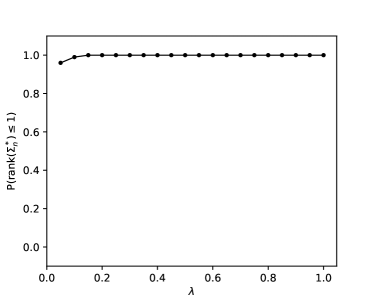
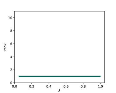
(a) $f(x)=x_{1}+x_{2}+x_{3}$.

(b) $f(x)=0.1(x_{1}+x_{2}+x_{3})^{3}+\tanh(x_{1}+x_{3}+x_{5})$.

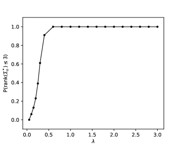
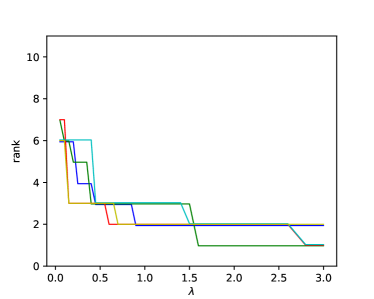
(c) $f(x)=2(x_{1}+x_{2})+(x_{2}+x_{3})^{2}+(x_{4}-0.5)^{3}$.

Figure 2: Plots for Claim (i). Here, we use Gaussian kernel $k_{\Sigma}(x,x^{\prime})=\exp\{-\left\|{x-x^{\prime}}\right\|_{\Sigma}^{2}\}$.
Experimental setting: the covariate $X\sim\mathsf{N}(0,I)$ and the response $Y=f(X)+\mathsf{N}(0,\sigma^{2})$ where $\sigma=0.1$. Here we choose $n=300$ and $p=50$. For each row, the left panel shows the empirical probability of ${\rm rank}(\Sigma_{n}^{*})\leq\dim(S_{*})$ over $100$ repeated experiments for different $\lambda$ values. The right panel displays how the rank of the solution $\Sigma_{n}^{*}$ changes with different $\lambda$ values, using $5$ example pairs of $(X,y)$.

8 Discussions

We would like to close this paper by offering a few comments about the results obtained in this paper and by discussing the possibility of generalizations and extensions.

8.1 Convergence Rates

The primary theoretical results in this paper concerning the empirical kernel learning objective are presented in an asymptotic fashion. For instance, in Theorem 1.2, we set $\lambda\in(0,\infty)$, and then consider $n\to\infty$.

For a deeper insight into the convergence rates of empirical minimizers, we require a nuanced nonasymptotic analysis. A key discovery in this paper is the sharpness property near optimal solutions of the population kernel learning objective (see Section 1.6.1). We plan to carry out a more refined nonasymptotic analysis that leverages this sharpness property to demonstrate that convergence rates mainly hinge on the intrinsic dimension, i.e., $\dim(S_{*})$, rather than the ambient dimension $p$.

8.2 Computation

An important question pertains to the computational aspects of minimizing the kernel learning objective (1.2). A promising idea is to use the random feature model to facilitate computations for kernel ridge regressions [RR07]. Our preliminary experiments suggest that the phenomenon persists in the relevant random feature model, although certain computational and statistical tradeoffs seem unavoidable. We hope to be able to report on these early findings in a follow-up paper.

8.3 Statistical Analysis of Local Minimum

While the primary objective of this paper is to characterize the low-rank nature of the global minimizer pertaining to the empirical objective $J_{n}$, comprehensive numerical experiments suggest for a wide range of distributions for $X$, the application of gradient descent on $J_{n}$ frequently results in matrices possessing exactly low rank. Since gradient descent’s convergence to global minimizers is not always guaranteed, our findings suggest that such low-rank properties might extend to local minimizers as well.

That being said, we hope to refine our analysis to gain a deeper understanding of the local minimizers for the kernel learning objective. Achieving this understanding may provide rigorous statistical guarantees for gradient-based algorithms targeting kernel learning.

9 Acknowledgements

The authors would like to thank X.Y. Han for enriching discussions on the experiments. Feng Ruan would like to thank Lijun Ding for his insightful comments on the initial draft, as well as to Basil Saeed, Lanqiu Yao, and Yuan Yao for their helpful discussions on the presentation.

Appendix A Proofs for Section 4

A.1 Proof of Lemma 4.1

We only prove the first statement of the lemma:

$$\sup_{U\in\mathsf{U}}\left|\!\left|\!\left|{\mathsf{C}_{U;\mathbb{P}_{n}}-\mathsf{C}_{U;\mathbb{P}}}\right|\!\right|\!\right|_{\rm op}=o_{P}(1).$$

Note the same idea leads to the proof of the second statement of Lemma 4.1.

In the proof below, we write $Q_{n}(U)=\left|\!\left|\!\left|{\mathsf{C}_{U;\mathbb{P}_{n}}-\mathsf{C}_{U;\mathbb{P}}}\right|\!\right|\!\right|_{\rm op}$ to simplify the notation.

According to [New91, Corollary 2.2], uniform convergence in probability holds if
(i) pointwise convergence holds, i.e., for every $U\in\mathsf{U}$, there’s the convergence

$$Q_{n}(U)=\left|\!\left|\!\left|{\mathsf{C}_{U;\mathbb{P}_{n}}-\mathsf{C}_{U;\mathbb{P}}}\right|\!\right|\!\right|_{\rm op}=o_{P}(1).$$

(ii) the random map $U\mapsto Q_{n}(U)$ satisfies the following uniform Lipschitz condition [New91, Corollary 2.2]: there is a sequence of random variables $B_{n}=O_{P}(1)$ such that

$$|Q_{n}(U)-Q_{n}(U^{\prime})|\leq B_{n}\times\left|\!\left|\!\left|{U-U^{\prime}}\right|\!\right|\!\right|_{\rm op}$$

holds for every $U,U^{\prime}\in\mathsf{U}$.

The pointwise convergence is known in the literature, e.g., [FBG07, Lemma 5].

It remains to prove the random map $U\mapsto Q_{n}(U)$ satisfies the uniform Lipschitz condition. The following lemma is crucial to this goal. It describes the Lipschitz property of $U\mapsto\mathsf{C}_{U;\mathbb{Q}}$ under a given measure $\mathbb{Q}$. The proof is given in Section A.1.1.

Lemma A.1 (Lipschitzness of $U\mapsto\mathsf{C}_{U;\mathbb{Q}}$).

For every $U,U^{\prime}\in\mathsf{U}$, and every measure $\mathbb{Q}$, we have

$$\left|\!\left|\!\left|{\mathsf{C}_{U;\mathbb{Q}}-\mathsf{C}_{U^{\prime};\mathbb{Q}}}\right|\!\right|\!\right|_{\rm op}\leq\sqrt{8\phi(0)|\phi^{\prime}_{+}(0)|}\cdot\left|\!\left|\!\left|{U-U^{\prime}}\right|\!\right|\!\right|_{\rm op}\cdot\sqrt{\mathbb{E}_{Q}[\left\|{X}\right\|_{2}^{2}]}.$$

For future reference, we document in parallel the Lipschitz property of $U\mapsto\mathsf{V}_{U;\mathbb{Q}}$.

Lemma A.2 (Lipschitzness of $U\mapsto\mathsf{V}_{U;\mathbb{Q}}$).

For every $U,U^{\prime}\in\mathsf{U}$, and every measure $\mathbb{Q}$, we have

$$\left|\!\left|\!\left|{\mathsf{V}_{U;\mathbb{Q}}-\mathsf{V}_{U^{\prime};\mathbb{Q}}}\right|\!\right|\!\right|_{\rm op}\leq\sqrt{8|\phi^{\prime}_{+}(0)|}\cdot\left|\!\left|\!\left|{U-U^{\prime}}\right|\!\right|\!\right|_{\rm op}\cdot\sqrt{\mathbb{E}_{Q}[\left\|{X}\right\|_{2}^{2}]}\cdot\sqrt{\mathbb{E}_{Q}[Y^{2}]}.$$

Back to the proof of the uniform Lipschitz condition. Following Lemma A.1, we obtain

$$|Q_{n}(U)-Q_{n}(U^{\prime})|\leq\left|\!\left|\!\left|{\mathsf{C}_{U;\mathbb{P}_{n}}-\mathsf{C}_{U^{\prime};\mathbb{P}_{n}}}\right|\!\right|\!\right|_{\rm op}+\left|\!\left|\!\left|{\mathsf{C}_{U;\mathbb{P}}-\mathsf{C}_{U^{\prime};\mathbb{P}}}\right|\!\right|\!\right|_{\rm op}\leq B_{n}\times\left|\!\left|\!\left|{U-U^{\prime}}\right|\!\right|\!\right|_{\rm op}$$

where

$$B_{n}=\sqrt{8\phi(0)|\phi^{\prime}_{+}(0)|}\cdot(\sqrt{\mathbb{E}_{P}[\left\|{X}\right\|_{2}^{2}]}+\sqrt{\mathbb{E}_{P_{n}}[\left\|{X}\right\|_{2}^{2}]}).$$

Note $B_{n}=O_{P}(1)$ as $\mathbb{E}_{P}[\left\|{X}\right\|_{2}^{2}]<\infty$. This established the desired uniform Lipschitz condition.

A.1.1 Proof of Lemma A.1

By definition, we have

$$\begin{split}\left|\!\left|\!\left|{\mathsf{C}_{U;\mathbb{Q}}-\mathsf{C}_{U^{\prime};\mathbb{Q}}}\right|\!\right|\!\right|_{\rm op}&=\sup_{\left\|{h_{1}}\right\|_{\mathcal{H}_{I}}\leq 1,\left\|{h_{2}}\right\|_{\mathcal{H}_{I}}\leq 1}|\langle h_{1},(\mathsf{C}_{U;\mathbb{Q}}-\mathsf{C}_{U^{\prime};\mathbb{Q}})h_{2}\rangle|\\ &=\sup_{\left\|{h_{1}}\right\|_{\mathcal{H}_{I}}\leq 1,\left\|{h_{2}}\right\|_{\mathcal{H}_{I}}\leq 1}|{\rm Cov}_{\mathbb{Q}}(h_{1}(U^{T}X),h_{2}(U^{T}X))-{\rm Cov}_{\mathbb{Q}}(h_{1}((U^{\prime})^{T}X),h_{2}((U^{\prime})^{T}X))|\end{split}$$

To bound the RHS, we need two properties that hold for every $f\in{\mathcal{H}_{I}}$ with $\left\|{f}\right\|_{\mathcal{H}_{I}}\leq 1$.

Lemma A.3.

For every $h\in\mathcal{H}_{I}$ with $\left\|{h}\right\|_{\mathcal{H}_{I}}\leq 1$,

1. ($L_{\infty}$ boundedness) $\left\|{h}\right\|_{\infty}\leq\sqrt{\phi(0)}$.

2. (Lipschitz property) $|h(x_{1})-h(x_{2})|\leq\sqrt{2|\phi_{+}^{\prime}(0)|}\cdot\left\|{x_{1}-x_{2}}\right\|_{2}$ holds for every $x_{1},x_{2}$.

Proof    The first property is due to the continuous embedding of $\mathcal{H}_{I}$ into $\mathsf{C}_{b}(\mathbb{R}^{p})$ (Proposition 1).

The second property is because of the following two inequalities. First, we use the reproducing property of the kernel $k$, and the Cauchy-Schwartz inequality to obtain for every $x_{1},x_{2}$

$$|h(x_{1})-h(x_{2})|=|\langle f,k_{I}(x_{1},\cdot)-k_{I}(x_{2},\cdot)\rangle_{\mathcal{H}_{I}}|\leq\left\|{h}\right\|_{\mathcal{H}_{I}}\times\left\|{k_{I}(x_{1},\cdot)-k_{I}(x_{2},\cdot)}\right\|_{\mathcal{H}_{I}}$$

Next, we use the reproducing property of the kernel $k$ again to derive the bound

$$\begin{split}\left\|{k_{I}(x_{1},\cdot)-k_{I}(x_{2},\cdot)}\right\|_{\mathcal{H}_{I}}^{2}&=k_{I}(x_{1},x_{1})+k_{I}(x_{2},x_{2})-2k_{I}(x_{1},x_{2})\\ &=2(\phi(0)-\phi(\left\|{x_{1}-x_{2}}\right\|_{2}^{2}))\leq 2\left\|{\phi^{\prime}}\right\|_{\infty}\left\|{x_{1}-x_{2}}\right\|^{2}.\end{split}$$

Note then $\left\|{\phi^{\prime}}\right\|_{\infty}\leq|\phi^{\prime}_{+}(0)|$. With these two inequalities, we derive the second property. ∎

Back to the proof of Lemma A.1. For every $h_{1},h_{2}\in{\mathcal{H}_{I}}$ with $\left\|{h_{1}}\right\|_{\mathcal{H}_{I}}\leq 1,\left\|{h_{2}}\right\|_{\mathcal{H}_{I}}\leq 1$, we have

$$\begin{split}&{\rm Cov}_{\mathbb{Q}}(h_{1}(U^{T}X),h_{2}(U^{T}X))-{\rm Cov}_{\mathbb{Q}}(h_{1}((U^{\prime})^{T}X),h_{2}((U^{\prime})^{T}X))\\ &={\rm Cov}_{\mathbb{Q}}(h_{1}(U^{T}X)-h_{1}((U^{\prime})^{T}X),h_{2}(U^{T}X))+{\rm Cov}_{\mathbb{Q}}(h_{1}((U^{\prime})^{T}X),h_{2}(U^{T}X)-h_{2}((U^{\prime})^{T}X))\\ \end{split}$$ (A.1)

Note then the first term on the RHS of equation (A.1) is bounded by

$$\begin{split}{\rm Cov}_{\mathbb{Q}}(h_{1}(U^{T}X)-h_{1}((U^{\prime})^{T}X),h_{2}(U^{T}X))&\leq\sqrt{\mathbb{E}_{Q}[(h_{1}(U^{T}X)-h_{1}((U^{\prime})^{T}X))^{2}]\times\mathbb{E}_{Q}[h_{2}^{2}(U^{T}X)]}\\ &\leq\sqrt{2|\phi_{+}^{\prime}(0)|\mathbb{E}_{Q}[\left\|{U^{T}X-(U^{\prime})^{T}X}\right\|_{2}^{2}]\times\phi(0)}\\ &\leq\sqrt{2|\phi_{+}^{\prime}(0)|\phi(0)}\cdot\left|\!\left|\!\left|{U-U^{\prime}}\right|\!\right|\!\right|_{\rm op}\cdot\sqrt{\mathbb{E}_{Q}[\left\|{X}\right\|_{2}^{2}]}.\end{split}$$

where the first inequality is due to Cauchy-Schwartz inequality, and the second inequality is due to Lemma A.3. The same bound holds for the second term on the RHS of equation (A.1). Together, this leads to the following desired bound that holds for every $U,U^{\prime}\in\mathsf{U}$:

$$\begin{split}\left|\!\left|\!\left|{\mathsf{C}_{U;\mathbb{Q}}-\mathsf{C}_{U^{\prime};\mathbb{Q}}}\right|\!\right|\!\right|_{\rm op}&\leq 2\sqrt{2|\phi_{+}^{\prime}(0)|\phi(0)}\cdot\left|\!\left|\!\left|{U-U^{\prime}}\right|\!\right|\!\right|_{\rm op}\cdot\sqrt{\mathbb{E}_{Q}[\left\|{X}\right\|_{2}^{2}]}.\end{split}$$

A.2 Proof of Lemma 4.6

For a given matrix $\Sigma\succeq 0$, let $U(\Sigma)=\Sigma^{1/2}$ denote the square root of the matrix $\Sigma$, which is defined as the unique positive semi-definite matrix $U$ satisfying $\Sigma=U^{2}$.

We initiate our proof with a bound on the gap of the residuals that holds for every $\Sigma,\Sigma^{\prime}$:

$$\left\|{r_{\Sigma;\mathbb{P}}-r_{\Sigma^{\prime};\mathbb{P}}}\right\|_{\infty}\leq 2\left\|{f_{U(\Sigma);\mathbb{P}}-f_{U(\Sigma^{\prime});\mathbb{P}}}\right\|_{\infty}\leq 2\sqrt{\phi(0)}\left\|{f_{U(\Sigma);\mathbb{P}}-f_{U(\Sigma^{\prime});\mathbb{P}}}\right\|_{\mathcal{H}_{I}}.$$ (A.2)

Here, the second inequality is due to the continuous embedding of the RKHS $\mathcal{H}_{I}$ into $\mathcal{C}_{b}(\mathbb{R}^{p})$, the space of all continuous functions equipped with $L_{\infty}$ norm (Proposition 1). Given the continuity of the square root mapping $\Sigma\mapsto U(\Sigma)$ on the set of positive semidefinite matrices [HJ12], to prove Lemma 4.6 it suffices to prove the continuity of $U\mapsto f_{U;\mathbb{P}}$ in the following sense:

$$\lim_{U^{\prime}\mapsto U}\left\|{f_{U^{\prime};\mathbb{P}}-f_{U;\mathbb{P}}}\right\|_{\mathcal{H}_{I}}=0.$$ (A.3)

We shall see that this follows from the continuity of the operator-valued mapping $U\mapsto\mathsf{C}_{U;\mathbb{P}}$ and the mapping $U\mapsto\mathsf{v}_{U;\mathbb{P}}$

$$\lim_{U^{\prime}\mapsto U}\left|\!\left|\!\left|{\mathsf{C}_{U^{\prime};\mathbb{P}}-\mathsf{C}_{U;\mathbb{P}}}\right|\!\right|\!\right|_{\rm op}=\lim_{U^{\prime}\mapsto U}\left\|{v_{U^{\prime};\mathbb{P}}-v_{U;\mathbb{P}}}\right\|_{\mathcal{H}_{I}}=0$$ (A.4)

which is further implied by the Lipschitzness property given in Lemma A.1 and Lemma A.2.

Indeed, by equation (4.9) there’s the identity that holds for every matrix $U,U^{\prime}\in\mathsf{U}$

$$f_{U;\mathbb{P}}=W(\mathsf{C}_{U;\mathbb{P}},v_{U;\mathbb{P}})~{}~{}\text{and}~{}~{}f_{U^{\prime};\mathbb{P}}=W(\mathsf{C}_{U^{\prime};\mathbb{P}},v_{U^{\prime};\mathbb{P}})$$

where $W:\mathsf{P}(\mathcal{H}_{I})\times\mathcal{H}_{I}\to\mathcal{H}_{I}$, as defined in equation (4.24), is continuous on its domain whenever $\lambda>0$ (recall $\mathcal{H}_{I}$ is equipped with the norm topology, $\mathsf{P}(\mathcal{H}_{I})\subseteq\mathsf{B}(\mathcal{H}_{I})$ is equipped with the subspace topology and the Cartesian product $\mathsf{P}(\mathcal{H}_{I})\times\mathcal{H}_{I}$ is equipped with the product topology). Hence, the desired continuity of $U\mapsto f_{U;\mathbb{P}}$ (equation (A.3)) is implied by that of the operators (equation (A.4)). The proof of Lemma 4.6 is thus complete.

Our proof strategy also implies the continuity of $\Sigma\mapsto J(\Sigma;\mathbb{P})$.

Lemma A.4 (Continuity of the Objective).

For every $\Sigma\in\mathsf{\Sigma}$, $\lim_{\Sigma^{\prime}\mapsto\Sigma}J(\Sigma^{\prime};\mathbb{P})=J(\Sigma;\mathbb{P})$.

Proof    Let $U(\Sigma)=\Sigma^{1/2}$ denote the square root of the matrix $\Sigma$, which is defined as the unique positive semi-definite matrix $U$ satisfying $\Sigma=U^{2}$. This mapping $\Sigma\mapsto U(\Sigma)$ is continuous on the set of positive definite matrices [HJ12].

By equation (4.10), there is the identity

$$|J(\Sigma;\mathbb{P})-J(\Sigma^{\prime};\mathbb{P})|=|T(\mathsf{C}_{U(\Sigma);\mathbb{P}},v_{U(\Sigma);\mathbb{P}})-T(\mathsf{C}_{U(\Sigma^{\prime});\mathbb{P}},v_{U(\Sigma^{\prime});\mathbb{P}})|$$ (A.5)

where $T:\mathsf{P}(\mathcal{H}_{I})\times\mathcal{H}_{I}\to\mathbb{R}$, as defined in equation (4.16), is continuous on its domain whenever $\lambda>0$ (recall $\mathcal{H}_{I}$ is equipped with the norm topology, $\mathsf{P}(\mathcal{H}_{I})\subseteq\mathsf{B}(\mathcal{H}_{I})$ is equipped with the subspace topology and the Cartesian product $\mathsf{P}(\mathcal{H}_{I})\times\mathcal{H}_{I}$ is equipped with the product topology). The continuity of the operator-valued mapping $U\mapsto\mathsf{C}_{U;\mathbb{P}}$ and the mapping $U\mapsto\mathsf{v}_{U;\mathbb{P}}$ described in equation (A.4) yields Lemma A.4 as desired. ∎

Appendix B Proof of Gradient Formula (Lemma 3.6)

Our proof below follows the main idea described in Section 3.3. Importantly, this proof is self-contained, meaning that it does not rely on any intermediate statements from Section 3.3.

Nonetheless, it is essential to note that our proof does depend on two specific results: Lemma 4.6 from Section 4 and Lemma A.4 from Section A. However, this dependency does not pose any issues because the proofs of these two lemmas do not, in any way, rely on the results from Section 3.

We shall first prove the gradient formula for positive definite $\Sigma\succ 0$.

Our first step is to rigorously justify the following property (cf. equation (3.25)).

Lemma B.1.

Given $\Sigma\succ 0$, there holds for all $\omega_{0}$ except for a set of Lebesgue measure $0$:

$$\mathbb{E}\left[r_{\Sigma}(X,Y)e^{-i\langle\omega_{0},X\rangle}\right]=\lambda\cdot\frac{\mathsf{F}{f}_{\Sigma}(\omega_{0})}{Q_{\Sigma}(\omega_{0})}.$$ (B.1)

Our second step is to rigorously justify the following property (cf. equation (3.22)).

Lemma B.2.

For every $\Sigma\succ 0$, the gradient $\nabla J(\Sigma)$ exists and satisfies

$$\nabla J(\Sigma)=-\frac{\lambda}{2}\int\frac{|\mathsf{F}f_{\Sigma}(\omega)|^{2}}{Q^{2}_{\Sigma}(\omega)}\partial_{\Sigma}Q_{\Sigma}(\omega)d\omega.$$ (B.2)

Now we are ready to prove the gradient formula for every $\Sigma\succ 0$. Fix $\Sigma\succ 0$. By taking the squared norm of both sides of equation (B.1) we obtain that

$$\mathbb{E}\left[r_{\Sigma}(X,Y)r_{\Sigma}(X^{\prime},Y^{\prime})e^{-i\langle\omega_{0},X-X^{\prime}\rangle}\right]=\lambda^{2}\cdot\frac{|\mathsf{F}f_{\Sigma}(\omega_{0})|^{2}}{Q^{2}_{\Sigma}(\omega_{0})}$$ (B.3)

holds almost everywhere $\omega_{0}$ under the Lebesgue measure. By substituting equation (B.3) into equation (B.2) we obtain

$$\begin{split}\nabla J(\Sigma)&=-\frac{1}{2\lambda}\int\mathbb{E}\left[r_{\Sigma}(X,Y)r_{\Sigma}(X^{\prime},Y^{\prime})e^{-i\langle\omega,X-X^{\prime}\rangle}\right]\partial_{\Sigma}Q_{\Sigma}(\omega)d\omega\\ &=-\frac{1}{2\lambda}\mathbb{E}\left[r_{\Sigma}(X,Y)r_{\Sigma}(X^{\prime},Y^{\prime})\int e^{-i\langle\omega,X-X^{\prime}\rangle}\partial_{\Sigma}Q_{\Sigma}(\omega)d\omega\right]\end{split}$$ (B.4)

By substituting $\partial_{\Sigma}k_{\Sigma}(x,x^{\prime})=\int e^{-i\langle\omega,x-x^{\prime}\rangle}\partial_{\Sigma}Q_{\Sigma}(\omega)d\omega$ into equation (B.4), we prove for $\Sigma\succ 0$

$$\nabla J(\Sigma)=-\frac{1}{2\lambda}\mathbb{E}[r_{\Sigma}(X;Y)r_{\Sigma}(X^{\prime};Y^{\prime})\partial_{\Sigma}k_{\Sigma}(X,X^{\prime})]$$ (B.5)

which is the desired gradient formula.

We shall next extend the gradient formula to every $\Sigma\succeq 0$. The following lemma is useful for this goal. Its proof is given in Section B.3.

Lemma B.3.

Suppose a continuous function $f:\mathcal{C}\mapsto\mathbb{R}$ has its gradient $\nabla f(\Sigma)=w(\Sigma)$ at every interior point $\Sigma\succ 0$. Suppose further that $\Sigma\mapsto w(\Sigma)$ is well-defined and continuous on $\mathcal{C}$. Then the function $f$ has gradient (Definition 3.1) given by $\nabla f(\Sigma)=w(\Sigma)$ at every $\Sigma\in\mathcal{C}$.

We apply Lemma B.3 to $J:\mathcal{C}\mapsto\mathbb{R}$. Note that $\Sigma\mapsto J(\Sigma)$ is continuous on $\mathcal{C}$ by Lemma A.4.

Let $w(\Sigma)=-\frac{1}{2\lambda}\mathbb{E}[r_{\Sigma}(X;Y)r_{\Sigma}(X^{\prime};Y^{\prime})\partial_{\Sigma}k_{\Sigma}(X,X^{\prime})]$ denote the RHS of equation (B.5). Previously, we have shown that $\nabla J(\Sigma)=w(\Sigma)$ for every $\Sigma\succ 0$.

Note the mapping $\Sigma\mapsto w(\Sigma)$ is well-defined and continuous on the entire convex set $\mathcal{C}$. In fact, the continuity of $\Sigma\mapsto w(\Sigma)$ follows from Lemma 4.6 and the continuity of $\Sigma\mapsto\partial_{\Sigma}k(x,x^{\prime})$.

By Lemma B.3, this shows that $J$ has the gradient $\nabla J(\Sigma)=w(\Sigma)$ at every $\Sigma\in\mathcal{C}$. Note $\nabla J$’s continuity follows from $w$ being continuous on $\mathcal{C}$. This completes the proof of Lemma 3.6.

B.1 Proof of Lemma B.1

According to the Euler-Lagrange equation (Lemma 3.5), we have for every $h\in\mathcal{H}_{\Sigma}$

$$\mathbb{E}[r_{\Sigma}(X,Y)h(X)]=\lambda\cdot\int\frac{\mathsf{F}f_{\Sigma}(\omega)\overline{\mathsf{F}h(\omega)}}{Q_{\Sigma}(\omega)}d\omega.$$ (B.6)

Recall that $\left\|{h}\right\|_{\mathcal{H}_{\Sigma}}^{2}=\int\frac{|\mathsf{F}h|^{2}(\omega)}{Q_{\Sigma}(\omega)}d\omega$ a real-valued function $h$. By decomposing a complex-valued function into real and imaginary parts, we can easily prove that

$$\mathbb{E}[r_{\Sigma}(X,Y)\overline{h(X)}]=\lambda\cdot\int\frac{\mathsf{F}f_{\Sigma}(\omega)\overline{\mathsf{F}h(\omega)}}{Q_{\Sigma}(\omega)}d\omega$$ (B.7)

holds for every $\mathbb{C}$-valued function $h$ satisfying $\int\frac{|\mathsf{F}h|^{2}(\omega)}{Q_{\Sigma}(\omega)}d\omega<\infty$.

For any $\omega_{0}$, let

$$h_{\omega_{0}}(x)=e^{i\langle\omega_{0},x\rangle}.$$

We want to mollify $h_{\omega_{0}}$ by $m_{\epsilon}$, which, for every $\epsilon>0$, is defined by

$$m_{\epsilon}(x)=\prod_{i=1}^{p}{\rm sinc}(\epsilon x_{i}).$$

In the above, ${\rm sinc}:\mathbb{R}\to\mathbb{R}$ is ${\rm sinc}(x)=\sin(x)/x$ for $x\neq 0$ and ${\rm sinc}(x)=1$ for $x=0$.

Write $h_{\omega_{0};\epsilon}=h_{\omega_{0}}m_{\epsilon}$. Note $\mathsf{F}m_{\epsilon}$ has compact support for $\epsilon>0$, as

$$\mathsf{F}m_{\epsilon}(\omega)=\begin{cases}\left(\frac{1}{2\epsilon}\right)^{p}~{}~{}&\text{if $\left\|{\omega}\right\|_{\infty}\leq\epsilon$}.\\ 0~{}~{}&\text{if otherwise}.\end{cases}$$

Hence, $\mathsf{F}h_{\omega_{0};\epsilon}(\cdot)=\mathsf{F}m_{\epsilon}(\cdot-\omega_{0})$ also has compact support. This implies that $\int\frac{|\mathsf{F}h_{\omega_{0};\epsilon}|^{2}(\omega)}{Q_{\Sigma}(\omega)}d\omega<\infty$ for every $\epsilon>0$.

We can thus substitute $h=h_{\omega_{0};\epsilon}$ into equation (B.7). This gives for every $\omega_{0}$ and $\epsilon>0$

$$\mathbb{E}[r_{\Sigma}(X,Y)\overline{h_{\omega_{0};\epsilon}(X)}]=\lambda\cdot\left(\frac{1}{2\epsilon}\right)^{p}\cdot\int_{\omega:\left\|{\omega-\omega_{0}}\right\|_{\infty}\leq\epsilon}\frac{\mathsf{F}f_{\Sigma}(\omega)}{Q_{\Sigma}(\omega)}d\omega.$$ (B.8)

Now, we take $\epsilon\to 0^{+}$ on both sides of equation (B.8).

Consider the LHS of equation (B.8) first. Note $\lim_{\epsilon\to 0^{+}}h_{\omega_{0};\epsilon}=h_{\omega_{0}}$ pointwise. Furthermore, there’s the domination $|r_{\Sigma}(x,y)h_{\omega_{0};\epsilon}(x)|\leq|r_{\Sigma}(x,y)|$ uniform over $\epsilon>0$ and that $\mathbb{E}[|r_{\Sigma}(X,Y)|]<\infty$ by Lemma 4.5. Hence, Lebesgue’s dominated convergence theorem yields for every $\omega_{0}$:

$$\lim_{\epsilon\to 0^{+}}\mathbb{E}[r_{\Sigma}(X,Y)\overline{h_{\omega_{0};\epsilon}(X)}]=\mathbb{E}[r_{\Sigma}(X,Y)\overline{h_{\omega_{0}}(X)}]=\mathbb{E}[r_{\Sigma}(X,Y)e^{-i\langle\omega_{0},X\rangle}].$$ (B.9)

Consider now the RHS of equation (B.8). Note first $\mathsf{F}f_{\Sigma}$ is $L_{1}$ integrable since $f_{\Sigma}\in\mathcal{H}_{\Sigma}$. Indeed,

$$\left\|{|\mathsf{F}f_{\Sigma}|}\right\|_{L_{1}(\mathbb{R}^{p})}\leq\left\|{\frac{|\mathsf{F}f_{\Sigma}|}{\sqrt{Q_{\Sigma}}}}\right\|_{L_{2}(\mathbb{R}^{p})}\cdot\left\|{\sqrt{Q_{\Sigma}}}\right\|_{L_{2}(\mathbb{R}^{p})}=\left\|{f_{\Sigma}}\right\|_{\mathcal{H}_{\Sigma}}\cdot\sqrt{\phi(0)}<\infty.$$

Thus the integrand $(\mathsf{F}f_{\Sigma}/Q_{\Sigma})(\omega)$ is locally $L_{1}$ integrable since $Q_{\Sigma}$ is locally bounded away from $0$. Hence, Lebesgue’s differentiable theorem for $L_{1}$ locally integrable function yields that

$$\lim_{\epsilon\to 0^{+}}\lambda\cdot\left(\frac{1}{2\epsilon}\right)^{p}\cdot\int_{\omega:\left\|{\omega-\omega_{0}}\right\|_{\infty}\leq\epsilon}\frac{\mathsf{F}f_{\Sigma}(\omega)}{Q_{\Sigma}(\omega)}d\omega=\lambda\cdot\frac{\mathsf{F}f_{\Sigma}(\omega_{0})}{Q_{\Sigma}(\omega_{0})},$$ (B.10)

which holds almost everywhere $\omega_{0}$ under the Lebesgue measure.

Lemma B.1 now follows from equations (B.8), (B.9) and (B.10).

B.2 Proof of Lemma B.2

Let us introduce

$$I(\Sigma,f,\gamma)=\frac{1}{2}\mathbb{E}[(Y-f(X)-\gamma)^{2}]+\frac{\lambda}{2}\left\|{f}\right\|_{\mathcal{H}_{\Sigma}}^{2}.$$ (B.11)

Then

$$J(\Sigma)=I(\Sigma,f_{\Sigma},\gamma_{\Sigma})=\min_{f,\gamma}I(\Sigma,f,\gamma).$$

We shall use the following form of envelope theorem to derive $\nabla J(\Sigma)$. Despite the wealth of study of envelope theorem, much is concerned with the case where the minimizing parameters are finite-dimensional, which does not fit our case since $f$ is infinite-dimensional. For completeness, we provide the proof of envelope theorem (Lemma B.4) in Section B.2.1.

Lemma B.4 (Envelope Theorem).

Let $v(x)=\min_{y}c(x,y)$ where $x\in\mathbb{R}^{k}$ is finite-dimensional and $y\in\mathsf{Y}$ where $\mathsf{Y}$ is any set. Fix $x_{0}$. Assume the following regularity conditions hold on some open neighborhood $\mathcal{N}(x_{0})$ of $x_{0}$.

• (Uniqueness of minimizer) There is a unique minimizer $y(x)$ of $\min_{y}c(x,y)$ for all $x\in\mathcal{N}(x_{0})$.

• (Existence of partial gradient) The partial gradient $\partial_{x}c(x^{\prime},y(x^{\prime\prime}))$ exists for all $x^{\prime},x^{\prime\prime}\in\mathcal{N}(x_{0})$.

• (Continuity of partial gradient) There is the limit $\lim_{x^{\prime}\to x_{0},x^{\prime\prime}\to x_{0}}\partial_{x}c(x^{\prime},y(x^{\prime\prime}))=\partial_{x}c(x_{0},y(x_{0}))$.

Then $v(x)$ is differentiable at $x_{0}$, with the gradient formula

$$\nabla v(x_{0})=\partial_{x}c(x_{0},y(x_{0})).$$

To apply the above envelope theorem (Lemma B.4) to derive the gradient of $J(\Sigma)=\min_{f,\gamma}I(\Sigma,f,\gamma)$, we need to verify the regularity conditions. Below, we fix $\Sigma_{0}\succ 0$.

Uniqueness of minimizer

This follows from standard arguments in learning theory, see, e.g., [CS02, Proposition 7]) and [CDV07, Proposition 1].

Existence of partial gradient

We shall prove $\partial_{\Sigma}I(\Sigma,f_{\Sigma^{\prime\prime}},\gamma_{\Sigma^{\prime\prime}})$ exists for all $\Sigma,\Sigma^{\prime\prime}$ close to $\Sigma_{0}$:

$$\partial_{\Sigma}I(\Sigma,f_{\Sigma^{\prime\prime}},\gamma_{\Sigma^{\prime\prime}})=\frac{\lambda}{2}\int\frac{|\mathsf{F}f_{\Sigma^{\prime\prime}}(\omega)|^{2}}{Q_{\Sigma}^{2}(\omega)}\partial_{\Sigma}Q_{\Sigma}(\omega)d\omega.$$ (B.12)

By definition of $I$ in equation (B.11), we need to show for every $\Sigma^{\prime\prime}$ near $\Sigma_{0}$, $\Sigma\mapsto\left\|{f_{\Sigma^{\prime\prime}}}\right\|_{\mathcal{H}_{\Sigma}}^{2}$ has gradient at every $\Sigma$ near $\Sigma_{0}$. Recall

$$\left\|{f_{\Sigma^{\prime\prime}}}\right\|_{\mathcal{H}_{\Sigma}}^{2}=\int\frac{|\mathsf{F}f_{\Sigma^{\prime\prime}}(\omega)|^{2}}{Q_{\Sigma}(\omega)}d\omega.$$ (B.13)

To show the gradient $\Sigma\mapsto\left\|{f_{\Sigma^{\prime\prime}}}\right\|_{\mathcal{H}_{\Sigma}}^{2}$ exists near $\Sigma_{0}$, our tool is Lemma B.5 whose textbook proof is based on Lebesgue’s dominated convergence theorem.

Lemma B.5 (Theorem 16.8 [Bil13]).

Fix $x_{0}$ and an open neighborhood $\mathcal{N}(x_{0})$ of $x_{0}$. Suppose that $b(x,\omega)$ is an $L_{1}$ integrable function of $\omega$ for $x\in\mathcal{N}(x_{0})$. Let $\phi(x)=\int b(x,\omega)d\omega$.

Suppose further that $\int\sup_{x\in\mathcal{N}(x_{0})}\left\|{\partial_{x}b(x,\omega)}\right\|_{2}d\omega<\infty$ holds. Then $\phi(x)$ is differentiable at every $x\in\mathcal{N}(x_{0})$, and its gradient satisfies $\nabla\phi(x)=\int\partial_{x}b(x,\omega)d\omega.$

Below we use Lemma B.5 to show the existence of gradient of $\Sigma\mapsto\left\|{f_{\Sigma^{\prime\prime}}}\right\|_{\mathcal{H}_{\Sigma}}^{2}$ for every $\Sigma^{\prime\prime}$ near $\Sigma_{0}$. Note first the integrand in equation (B.13) has the following partial gradient

$$\partial_{\Sigma}\frac{|\mathsf{F}f_{\Sigma^{\prime\prime}}(\omega)|^{2}}{Q_{\Sigma}(\omega)}=\frac{|\mathsf{F}f_{\Sigma^{\prime\prime}}(\omega)|^{2}}{Q_{\Sigma}^{2}(\omega)}\partial_{\Sigma}Q_{\Sigma}(\omega).$$

By Lemma B.1, the following holds for all $\omega$ except for a set of Lebesgue measure $0$:

$$\mathsf{F}f_{\Sigma}(\omega)=\frac{1}{\lambda}\cdot Q_{\Sigma}(\omega)\cdot\mathbb{E}[r_{\Sigma}(X,Y)e^{i\langle\omega,X\rangle}].$$ (B.14)

By Lemma 4.5, $\mathbb{E}[|r_{\Sigma}(X,Y)|]\leq\sqrt{{\rm Var}(Y)}$. This proves for every $\Sigma$,

$$|\mathsf{F}f_{\Sigma}(\omega)|\leq\frac{1}{\lambda}\sqrt{{\rm Var}(Y)}\cdot Q_{\Sigma}(\omega)$$ (B.15)

holds almost everywhere $\omega$ under the Lebesgue measure.

Now we need the following integrability result regarding $Q_{\Sigma}$. The proof of Lemma B.6 can be found in Section B.4.

Lemma B.6.

For any $\Sigma_{0}\succ 0$, there exists a neighborhood $\mathcal{N}(\Sigma_{0})$ of $\Sigma_{0}$ such that

$$\int\sup_{\Sigma,\Sigma^{\prime\prime}\in\mathcal{N}(\Sigma_{0})}\left|\!\left|\!\left|{\frac{Q^{2}_{\Sigma^{\prime\prime}}(\omega)}{Q_{\Sigma}^{2}(\omega)}\partial_{\Sigma}Q_{\Sigma}(\omega)}\right|\!\right|\!\right|_{F}d\omega<\infty$$ (B.16)

Given Lemma B.6 and the pointwise bound (B.15), we can apply Lemma B.5 to show there is the existence of gradient of $\Sigma\mapsto\left\|{f_{\Sigma^{\prime\prime}}}\right\|_{\mathcal{H}_{\Sigma}}^{2}$ when $\Sigma,\Sigma^{\prime\prime}\in\mathcal{N}(\Sigma_{0})$, and that gradient satisfies

$$\partial_{\Sigma}(\left\|{f_{\Sigma^{\prime\prime}}}\right\|_{\mathcal{H}_{\Sigma}}^{2})=\partial_{\Sigma}\int\frac{|\mathsf{F}f_{\Sigma^{\prime\prime}}(\omega)|^{2}}{Q_{\Sigma}(\omega)}d\omega=\int\frac{|\mathsf{F}f_{\Sigma^{\prime\prime}}(\omega)|^{2}}{Q_{\Sigma}^{2}(\omega)}\partial_{\Sigma}Q_{\Sigma}(\omega)d\omega.$$ (B.17)

This proves $\partial_{\Sigma}I(\Sigma,f_{\Sigma^{\prime\prime}},\gamma_{\Sigma^{\prime\prime}})$ exists with $\partial_{\Sigma}I(\Sigma,f_{\Sigma^{\prime\prime}},\gamma_{\Sigma^{\prime\prime}})=\frac{\lambda}{2}\partial_{\Sigma}(\left\|{f_{\Sigma^{\prime\prime}}}\right\|_{\mathcal{H}_{\Sigma}}^{2})$ for $\Sigma,\Sigma^{\prime\prime}\in\mathcal{N}(\Sigma_{0})$.

Continuity of partial gradient

We shall prove the following statement:

$$\lim_{\Sigma\to\Sigma_{0},\Sigma^{\prime\prime}\to\Sigma_{0}}\partial_{\Sigma}I(\Sigma,f_{\Sigma^{\prime\prime}},\gamma_{\Sigma^{\prime\prime}})=\partial_{\Sigma}I(\Sigma_{0},f_{\Sigma_{0}},\gamma_{\Sigma_{0}}).$$ (B.18)

By expression (B.12), this is equivalent to show:

$$\lim_{\Sigma\to\Sigma_{0},\Sigma^{\prime\prime}\to\Sigma_{0}}\int\frac{|\mathsf{F}f_{\Sigma^{\prime\prime}}(\omega)|^{2}}{Q_{\Sigma}^{2}(\omega)}\partial_{\Sigma}Q_{\Sigma}(\omega)d\omega=\int\frac{|\mathsf{F}f_{\Sigma_{0}}(\omega)|^{2}}{Q_{\Sigma_{0}}^{2}(\omega)}(\partial_{\Sigma}Q_{\Sigma}(\omega)\mid_{\Sigma=\Sigma_{0}})d\omega.$$ (B.19)

Above, $\partial_{\Sigma}Q_{\Sigma}(\omega)\mid_{\Sigma=\Sigma_{0}}$ denotes the partial gradient of $Q_{\Sigma}(\omega)$ with respect to $\Sigma$ evaluated at $\Sigma=\Sigma_{0}$.

Our proof leverages Lemma B.1 and Lebesgue’s dominated convergence theorem. By taking the square of both sides of (B.14), we obtain, for $(X^{\prime},Y^{\prime})$ independent copy of $(X,Y)$:

$$z_{\Sigma}(\omega):=\mathbb{E}\left[r_{\Sigma}(X,Y)r_{\Sigma}(X^{\prime},Y^{\prime})e^{-i\langle\omega,X-X^{\prime}\rangle}\right]=\lambda\cdot\frac{|\mathsf{F}{f}_{\Sigma}(\omega)|^{2}}{Q_{\Sigma}^{2}(\omega)}$$

holds for almost everywhere $\omega$. Thus to prove our target equation (B.19) it suffices to show

$$\lim_{\Sigma\to\Sigma_{0},\Sigma^{\prime\prime}\to\Sigma_{0}}\int|z_{\Sigma^{\prime\prime}}(\omega)|^{2}\frac{Q^{2}_{\Sigma^{\prime\prime}}(\omega)}{Q_{\Sigma}^{2}(\omega)}\partial_{\Sigma}Q_{\Sigma}(\omega)d\omega=\int|z_{\Sigma_{0}}(\omega)|^{2}\frac{Q^{2}_{\Sigma_{0}}(\omega)}{Q_{\Sigma_{0}}^{2}(\omega)}(\partial_{\Sigma}Q_{\Sigma}(\omega)\mid_{\Sigma=\Sigma_{0}})d\omega$$ (B.20)

This is achieved by invoking Lebesgue’s dominated convergence theorem. Indeed,

• (Continuity) $\lim_{\Sigma^{\prime\prime}\to\Sigma_{0}}z_{\Sigma}(\omega)=z_{\Sigma_{0}}(\omega)$ holds for all $\omega$ due to the continuity of $\Sigma\mapsto r_{\Sigma}$ stated in Lemma 4.6. Moreover, $(\Sigma,\Sigma^{\prime\prime})\mapsto\frac{Q^{2}_{\Sigma^{\prime\prime}}(\omega)}{Q_{\Sigma}^{2}(\omega)}\partial_{\Sigma}Q_{\Sigma}(\omega)$ is continuous near $(\Sigma_{0},\Sigma_{0})$

• (Domination) Note $|z_{\Sigma}(\omega)|\leq\sqrt{{\rm Var}(Y)}$ holds uniformly over $\Sigma,\omega$ by Lemma 4.5. Also, by Lemma B.6, there’s some neighborhood $\mathcal{N}(\Sigma_{0})$ of $\Sigma_{0}$ such that

  $$\int\sup_{\Sigma,\Sigma^{\prime\prime}\in\mathcal{N}(\Sigma_{0})}\left|\!\left|\!\left|{\frac{Q^{2}_{\Sigma^{\prime\prime}}(\omega)}{Q_{\Sigma}^{2}(\omega)}\partial_{\Sigma}Q_{\Sigma}(\omega)}\right|\!\right|\!\right|_{F}d\omega<\infty$$

Summary

Having met all required conditions, we can use Lemma B.4 to affirm the gradient existence of $J(\Sigma)=\min_{f,\gamma}I(\Sigma,f,\gamma)$ when $\Sigma\in\mathcal{C}$. Furthermore, that gradient satisfies

$$\nabla J(\Sigma)=-\frac{\lambda}{2}\int\frac{|\mathsf{F}f_{\Sigma}(\omega)|^{2}}{Q^{2}_{\Sigma}(\omega)}\partial_{\Sigma}Q_{\Sigma}(\omega)d\omega.$$

B.2.1 Proof of Lemma B.4

For any $x\in\mathcal{N}(x_{0})$, by Taylor’s intermediate theorem, there is $\underline{x}$ on the segment of $x_{0}$ and $x$ such that $v(x)=c(x,y(x))=c(x_{0},y(x))+\langle\partial_{x}c(\underline{x},y(x)),x-x_{0}\rangle$ holds. Note $c(x_{0},y(x))\geq c(x_{0},y(x_{0}))$. Together, they imply

$$\begin{split}v(x)&\geq c(x_{0},y(x_{0}))+\langle\partial_{x}c(\underline{x},y(x)),x-x_{0}\rangle\\ &=c(x_{0},y(x_{0}))+\langle\partial_{x}c(x_{0},y(x_{0})),x-x_{0}\rangle+o(\left\|{x-x_{0}}\right\|).\end{split}$$ (B.21)

The last line uses $\lim_{x_{1}\to x_{0},x_{2}\to x_{0}}\partial c(x_{1},y(x_{2}))=\partial c(x_{0},y(x_{0}))$ assumed in Lemma B.4.

Similarly, $v(x)=c(x,y(x))\leq c(x,y(x_{0}))$ by definition. Furthermore, by Taylor’s intermediate theorem, there is $\bar{x}$ such that $c(x,y(x_{0}))=c(x_{0},y(x_{0}))+\langle\partial_{x}c(\bar{x},y(x_{0})),x-x_{0}\rangle$. This yields

$$\begin{split}v(x)&\leq c(x_{0},y(x_{0}))+\langle\partial_{x}c(\bar{x},y(x_{0})),x-x_{0}\rangle\\ &=c(x_{0},y(x_{0}))+\langle\partial_{x}c(x_{0},y(x_{0})),x-x_{0}\rangle+o(\left\|{x-x_{0}}\right\|).\end{split}$$ (B.22)

The above lower and upper bounds imply there’s the identity:

$$v(x)=c(x_{0},y(x_{0}))+\langle\partial_{x}c(x_{0},y(x_{0})),x-x_{0}\rangle+o(\left\|{x-x_{0}}\right\|).$$

This proves that $v$ is differentiable at $x_{0}$, with $\nabla v(x_{0})=\partial_{x}c(x_{0},y(x_{0}))$.

B.3 Proof of Lemma B.3

Our proof is based on convex and mathematical analysis.

Fix $\Sigma\in\mathop{\rm bd}(\mathcal{C})$ where $\mathop{\rm bd}(\mathcal{C})$ denotes the boundary of the set $\mathcal{C}$. Let $\Sigma_{n}\to\Sigma$ where $\Sigma_{n}\in\mathcal{C}$. We shall prove

$$f(\Sigma_{n})=f(\Sigma)+\langle w(\Sigma),\Sigma_{n}-\Sigma\rangle+o(\left|\!\left|\!\left|{\Sigma_{n}-\Sigma}\right|\!\right|\!\right|_{F}).$$

First, we assume temporarily that $\Sigma_{n}\succ 0$ for every $n\in\mathbb{N}$. Denote $\Sigma_{n}(t)=t\Sigma+(1-t)\Sigma_{n}$ for every $t\in[0,1]$. Since $\mathcal{C}$ is convex, $\Sigma_{n}(t)\succ 0$ when $t\in[0,1)$. Since the function $f$ is continuous and differentiable, whose gradient $\nabla f$ agrees with $w$ within the interior of $\mathcal{C}$, the fundamental theorem of calculus yields

$$\begin{split}f(\Sigma_{n})&=f(\Sigma)+\int_{0}^{1}\langle w(\Sigma_{n}(t)),\Sigma_{n}-\Sigma\rangle dt\\ &=f(\Sigma)+\langle w(\Sigma),\Sigma_{n}-\Sigma\rangle+o(\left|\!\left|\!\left|{\Sigma_{n}-\Sigma}\right|\!\right|\!\right|_{F}).\end{split}$$

where the second identity uses that $w$ is continuous at $\Sigma$.

The general case where $\Sigma_{n}\in\mathcal{C}$ follows from a perturbation argument. Since $f$ is continuous, we can find $\Sigma_{n}^{\prime}\succ 0$ such that $\left|\!\left|\!\left|{\Sigma_{n}^{\prime}-\Sigma_{n}}\right|\!\right|\!\right|=o(\left|\!\left|\!\left|{\Sigma_{n}-\Sigma}\right|\!\right|\!\right|_{F})$ and $|f(\Sigma_{n}^{\prime})-f(\Sigma_{n})|=o(\left|\!\left|\!\left|{\Sigma_{n}-\Sigma}\right|\!\right|\!\right|_{F})$. Applying the previous result to $\Sigma_{n}^{\prime}$, we obtain $f(\Sigma_{n}^{\prime})=f(\Sigma)+\langle w(\Sigma),\Sigma_{n}^{\prime}-\Sigma\rangle+o(\left|\!\left|\!\left|{\Sigma_{n}^{\prime}-\Sigma}\right|\!\right|\!\right|_{F})$. Note by triangle inequality this further implies $f(\Sigma_{n})=f(\Sigma)+\langle w(\Sigma),\Sigma_{n}-\Sigma\rangle+o(\left|\!\left|\!\left|{\Sigma_{n}-\Sigma}\right|\!\right|\!\right|_{F})$.

B.4 Proof of Lemma B.6

The proof is based on a series of estimates.

First, we have the estimate on $\partial_{\Sigma}Q_{\Sigma}$. There exists $c(\Sigma)<\infty$ continuous at $\Sigma_{0}\succ 0$ such that

$$\left\|{\partial_{\Sigma}Q_{\Sigma}(\omega)}\right\|_{F}\leq c(\Sigma)(1+\left\|{\omega}\right\|_{2}^{2})Q_{\Sigma}(\omega)$$

holds for every $\omega$ and all $\Sigma$ that is within a neighborhood near $\Sigma_{0}$. With this estimate, it suffices to prove for some neighborhood $\mathcal{N}(\Sigma_{0})$ around $\Sigma_{0}$:

$$\int\sup_{\Sigma,\Sigma^{\prime\prime}\in\mathcal{N}(\Sigma_{0})}\left|\!\left|\!\left|{\frac{Q^{2}_{\Sigma^{\prime\prime}}(\omega)}{Q_{\Sigma}(\omega)}(1+\left\|{\omega}\right\|_{2}^{2})}\right|\!\right|\!\right|_{F}d\omega<\infty$$ (B.23)

Next, we provide an estimate on $\frac{Q^{2}_{\Sigma^{\prime\prime}}(\omega)}{Q_{\Sigma}(\omega)}$ for every $\Sigma,\Sigma^{\prime\prime}$. Our main idea is to apply the Cauchy Schwartz inequality to the integral representation (2.2). To make it concrete, we note that

$$Q_{\Sigma}(\omega)=C(\Sigma)\cdot\int_{0}^{\infty}z(t;\Sigma)\mu(dt)~{}~{}\text{where}~{}~{}z(t;\Sigma)=\left(\frac{1}{t}\right)^{p/2}e^{-\left\|{w}\right\|_{(4t\Sigma)^{-1}}^{2}}$$

where $C(\Sigma)=(\frac{1}{4\pi})^{p/2}\cdot\frac{1}{|\det\Sigma|^{1/2}}$. The key is for $\Sigma_{1},\Sigma_{2},\Sigma_{3}$ obeying $\Sigma_{1}^{-1}+\Sigma_{3}^{-1}=2\Sigma_{2}^{-1}$,

$$\left(\int_{0}^{\infty}z(t;\Sigma_{2})\mu(dt)\right)^{2}\leq\int_{0}^{\infty}z(t;\Sigma_{1})\mu(dt)\int_{0}^{\infty}z(t;\Sigma_{3})\mu(dt)~{}\text{for every $\omega$},$$

by the Cauchy-Schwartz inequality, which we can leverage to show that there is a neighborhood $\mathcal{N}(\Sigma_{0})$ of $\Sigma_{0}$ and a sufficient small $\underline{c}>0$ and large $\underline{C}>0$ such that for every $\omega$

$$\sup_{\Sigma,\Sigma^{\prime\prime}\in\mathcal{N}(\Sigma_{0})}\left|\frac{Q^{2}_{\Sigma^{\prime\prime}}(\omega)}{Q_{\Sigma}(\omega)}\right|\leq\underline{C}Q_{\underline{c}I}(\omega)$$

Thus we can use these estimates to conclude for some neighborhood $\mathcal{N}(\Sigma_{0})$ of $\Sigma_{0}$:

$$\int\sup_{\Sigma,\Sigma^{\prime\prime}\in\mathcal{N}(\Sigma_{0})}\left|\!\left|\!\left|{\frac{Q^{2}_{\Sigma^{\prime\prime}}(\omega)}{Q_{\Sigma}(\omega)}(1+\left\|{\omega}\right\|_{2}^{2})}\right|\!\right|\!\right|_{F}d\omega\leq\underline{C}\int Q_{\underline{c}I}(\omega)(1+\left\|{\omega}\right\|_{2}^{2})d\omega.$$

Lastly the last integral $\int Q_{\underline{c}I}(\omega)(1+\left\|{\omega}\right\|_{2}^{2})d\omega$ is bounded because $\phi$ is differentiable on $[0,\infty)$. Indeed, one can first show that $\int_{0}^{\infty}t\mu(dt)<\infty$ because $\phi_{+}^{\prime}(0)$ exists, and then use this to show

$$\int Q_{\underline{c}I}(\omega)(1+\left\|{\omega}\right\|_{2}^{2})d\omega=C(\underline{c}I)\cdot\int_{0}^{\infty}\int z(t;\underline{c}I)(1+\left\|{\omega}\right\|_{2}^{2})d\omega\mu(dt)\leq C^{\prime\prime}\int_{0}^{\infty}t\mu(dt)<\infty.$$

In the above, $C^{\prime\prime}<\infty$ depend on $C(\underline{c}I)$, $\underline{c}$ and $m_{\mu}$ where we recall $\mathop{\rm supp}(\mu)\subseteq[m_{\mu},\infty)$.

Appendix C Proof of Lemma in Section 3

C.1 Proof of Lemma 3.1

Let $\Sigma=UU^{T}\succeq 0$.

The key instrument in our proof is the representer theorem, which states that the minimizer of a kernel ridge regression can be expressed as a linear combination of the kernel functions [KW70, SHS01].

Let $g_{U},\gamma_{U}$ be the minimum of the cost function defining $H$ (3.3). The associated representer theorem for kernel ridge regression with $H$ is given below.

Lemma C.1 (representer theorem for $H$).

$g_{U}(\cdot)=\mathbb{E}[a(X)k_{I}(U^{T}X,\cdot)]$ for some $a\in\mathcal{L}_{2}(\mathbb{P})$.

Proof    Taking the first variation of the cost function in (3.3) with respect to $g$, we get that for $r_{U}(x,y)=y-g_{U}(U^{T}x)-\gamma_{U}$, the following identity is true:

$$\mathbb{E}[r_{U}(X,Y)h(U^{T}X)]=\lambda\langle g_{U},h\rangle~{}~{}\text{holds for every $h\in\mathcal{H}_{I}$}.$$

Observe that the left-hand side is equal to $\langle\mathbb{E}[r_{U}(X,Y)k_{I}(U^{T}X,\cdot)],h\rangle_{\mathcal{H}_{I}}$ due to the reproducing property of $k_{I}$.

Since the identity is valid for all $h\in\mathcal{H}_{I}$, it implies that $g_{U}(\cdot)=\mathbb{E}[r_{U}(X,Y)k_{I}(U^{T}X,\cdot)]$. Therefore, $g_{U}(\cdot)=\mathbb{E}[a(X)k(U^{T}X,\cdot)]$ where $a(x)=\frac{1}{\lambda}\mathbb{E}[r_{U}(X,Y)|X=x]$ and $a\in\mathcal{L}_{2}(\mathbb{P})$.

∎

Similarly, we have the representer theorem for the kernel ridge regression associated with $J$.

Lemma C.2 (representer theorem for $J$).

$f_{\Sigma}(\cdot)=\mathbb{E}[a(X)k_{\Sigma}(X,\cdot)]$ for some $a\in\mathcal{L}_{2}(\mathbb{P})$.

Let $(X^{\prime},Y^{\prime})$ be an independent copy of $(X,Y)$.

Using Lemma C.1, we can express $H$ as follows:

$$\begin{split}H(U)&=\min_{g,\gamma}\frac{1}{2}\mathbb{E}[(Y-g(U^{T}X)-\gamma)^{2}]+\frac{\lambda}{2}\left\|{g}\right\|_{\mathcal{H}_{I}}^{2}\\ &=\min_{a\in\mathcal{L}_{2}(\mathbb{P}),\gamma\in\mathbb{R}}\frac{1}{2}\mathbb{E}[(Y-\mathbb{E}[a(X^{\prime})k_{I}(U^{T}X^{\prime},U^{T}X)]-\gamma)^{2}]+\frac{\lambda}{2}\mathbb{E}[a(X)a(X^{\prime})k_{I}(U^{T}X^{\prime},U^{T}X)].\end{split}$$

Basically, we replace $g(\cdot)=\mathbb{E}[a(X^{\prime})k_{I}(U^{T}X^{\prime},\cdot)$ in the first line to obtain the second line.

Similarly, using Lemma C.2, we can express $J$ as:

$$J(\Sigma)=\min_{a\in\mathcal{L}_{2}(\mathbb{P}),\gamma\in\mathbb{R}}\frac{1}{2}\mathbb{E}[(Y-\mathbb{E}[a(X^{\prime})k_{\Sigma}(X^{\prime},X)]-\gamma)^{2}]+\frac{\lambda}{2}\mathbb{E}[a(X)a(X^{\prime})k_{\Sigma}(X^{\prime},X)].$$

It is then clear that $J(\Sigma)=H(U)$, since $k_{I}(U^{T}x,U^{T}x^{\prime})=k_{\Sigma}(x,x^{\prime})$ for all $x,x^{\prime}$ when $\Sigma=UU^{T}$.

C.2 Proof of Lemma 3.4

Recall $\epsilon_{0}(S)=\mathbb{E}[{\rm Var}(Y|\Pi_{S}X)]-\mathbb{E}[{\rm Var}(Y|X)]$. By bias-variance decomposition (or ANOVA),

$$\epsilon_{0}(S)=\mathbb{E}[(\mathbb{E}[Y|\Pi_{S}X]-\mathbb{E}[Y|X])^{2}].$$

Hence, $\epsilon_{0}(S)>0$ for every subspace $S$ with $\dim(S)<\dim(S_{*})$.

To prove Lemma 3.4, it is sufficient to show that

$$\inf\{\epsilon_{0}(S)|\dim(S)<\dim(S_{*})\}>0.$$ (C.1)

Our proof is by contradiction and uses a standard compactness argument.

Assume, for the sake of contradiction, that the infimum in (C.1) is zero. Then there exists a sequence of subspaces $S_{n}$ such that $\epsilon_{0}(S_{n})$ converges to $0$ with $\dim(S_{n})<\dim(S_{*})$.

First, because the set of projection matrices is compact, we may, by taking a subsequence if necessary, assume that $\Pi_{S_{n}}\to\Pi_{S_{\infty}}$ holds for some subspace $S_{\infty}$ with $\dim(S_{\infty})<\dim(S_{*})$.

Next, define for every $n<\infty$

$$\phi_{n}(X)=\mathbb{E}[Y|\Pi_{S_{n}}X]-\mathbb{E}[Y|X].$$

Note $\phi_{n}$ is uniformly bounded in $\mathcal{L}_{2}(\mathbb{P})$. By the Banach-Alaoglu theorem, the unit ball in $\mathcal{L}_{2}(\mathbb{P})$ is weak-* sequentially compact, so, by taking a subsequence if necessary, we may assume that $\phi_{n}$ converges to some $\phi_{\infty}$ in $\mathcal{L}_{2}(\mathbb{P})$ under the weak-* topology, i.e., $\mathbb{E}[\phi_{n}(X)h(X)]\to\mathbb{E}[\phi_{\infty}(X)h(X)]$ holds for every $h\in\mathcal{L}_{2}(\mathbb{P})$.

We then prove two claims: (a) $\phi_{\infty}(X)=\mathbb{E}[Y|\Pi_{S_{\infty}}X]-\mathbb{E}[Y|X]$, and (b) $\mathbb{E}[\phi_{\infty}^{2}(X)]=0$. This would imply that $\epsilon_{0}(S_{\infty})=0$ even though $\dim(S_{\infty})<\dim(S_{*})$, which contradicts the definition of $S_{*}$. Therefore, the infimum in (C.1) must be thereby strictly positive, and Lemma 3.4 is proved.

To prove (a), let’s denote $\gamma_{n}(X)=\mathbb{E}[Y|\Pi_{S_{n}}X]$. It suffices to show that any accumulation point $\gamma_{\infty}$ of $\gamma_{n}$ in $\mathcal{L}_{2}(\mathbb{P})$ under the weak-* topology must satisfy $\gamma_{\infty}(X)=\mathbb{E}[Y|\Pi_{S_{\infty}}X]$. To show this, it suffices to prove that any such accumulation point $\gamma_{\infty}$ satisfies the orthogonality condition

$$\mathbb{E}[(Y-\gamma_{\infty}(X))h(\Pi_{S_{\infty}}X)]=0$$ (C.2)

for every continuous function $h$ that is uniformly bounded on $\mathbb{R}^{p}$. Since $\mathbb{E}[(Y-\gamma_{n}(X))h(\Pi_{S_{n}}X)]=0$ for every $n$ and $h(\Pi_{S_{n}}X)$ converge to $h(\Pi_{S_{\infty}}X)$ in $\mathcal{L}_{2}(\mathbb{P})$ under the norm topology for every such function $h$, the desired orthogonality condition (C.2) follows by letting $n\to\infty$.

To prove (b), note by Cauchy-Schwartz $\mathbb{E}[\phi_{n}(X)\phi_{\infty}(X)]\to 0$ as $\mathbb{E}[\phi_{n}^{2}(X)]=\epsilon_{0}(S_{n})\to 0$. That $\mathbb{E}[\phi_{\infty}^{2}(X)]=0$ now follows from the convergence of $\phi_{n}$ to $\phi_{\infty}$ under the weak-* topology in $\mathcal{L}_{2}(\mathbb{P})$.

This completes the proof of Lemma 3.4.

Appendix D Additional Plots

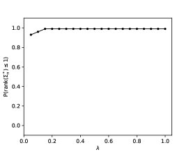
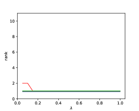
(a) $f(x)=x_{1}+x_{2}+x_{3}$.

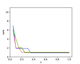
(b) $f(x)=x_{1}x_{2}$.

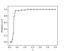
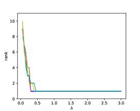
(c) $f(x)=0.1(x_{1}+x_{2}+x_{3})^{3}+\tanh(x_{1}+x_{3}+x_{5})$.

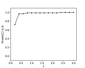
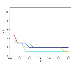
(d) $f(x)=2(x_{1}+x_{2})+(x_{2}+x_{3})^{2}+(x_{4}-0.5)^{3}$.

Figure 3: Plots for Claim (ii). Here, we use Gaussian kernel $k_{\Sigma}(x,x^{\prime})=\exp\{-\left\|{x-x^{\prime}}\right\|_{\Sigma}^{2}\}$.
Experimental setting: the covariate $X\sim\mathsf{N}(0,K)$, with $K_{i,j}=0.5^{|i-j|}$ and the response follows $Y=f(X)+\mathsf{N}(0,\sigma^{2})$ where $\sigma=0.1$. Here, we set $n=300$ and $p=50$.
For each row, the left panel shows the empirical probability of ${\rm rank}(\Sigma_{n}^{*})\leq\dim(S_{*})$ over $100$ repeated experiments for different $\lambda$ values. The right panel displays how the rank of the solution $\Sigma_{n}^{*}$ changes with different $\lambda$ values, using $5$ example pairs of $(X,y)$.

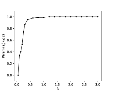
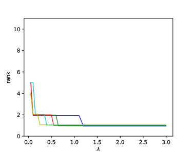
(a) Discrete $X$, $f(x)=0.1(x_{1}+x_{2}+x_{3})^{3}+\tanh(x_{1}+x_{3}+x_{5})$.

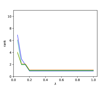
(b) Continuous $X$, $f(x)=0.1(x_{1}+x_{2}+x_{3})^{3}+\tanh(x_{1}+x_{3}+x_{5})$.

Figure 4: Plots for Claim (iii). Here, we use Gaussian kernel $k_{\Sigma}(x,x^{\prime})=\exp\{-\left\|{x-x^{\prime}}\right\|_{\Sigma}^{2}\}$.
Experimental setting: the covariate $X$ has independent coordinates $X_{i}$, with each $X_{i}$ obeying $\mathbb{P}(X_{i}=1)=\mathbb{P}(X_{i}=0)=0.5$ in the discrete setting, and being uniform on $[0,1]$ in the continuous setting, and the response follows $Y=f(X)+\mathsf{N}(0,\sigma^{2})$ where $\sigma=0.1$. Here, we set $n=300$ and $p=50$.
For each row, the left panel shows the empirical probability of ${\rm rank}(\Sigma_{n}^{*})\leq\dim(S_{*})$ over $100$ repeated experiments for different $\lambda$ values. The right panel displays how the rank of the solution $\Sigma_{n}^{*}$ changes with different $\lambda$ values, using $5$ example pairs of $(X,y)$.

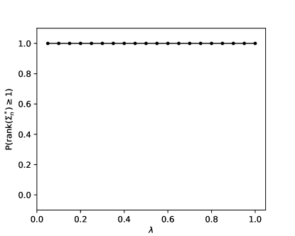
Figure 5: Plot for Claim (iv). Here, we use Gaussian kernel $k_{\Sigma}(x,x^{\prime})=\exp\{-\left\|{x-x^{\prime}}\right\|_{\Sigma}^{2}\}$.
In this experiment, ${\rm Var}(\mathbb{E}[Y|X])=0$ where $X\sim\mathsf{N}(0,I)$, and $Y=\epsilon$, where $\epsilon\sim\mathsf{N}(0,\sigma^{2})$ is independent of $X$ with $\sigma=0.1$. Here, we choose $n=300$ and $p=50$.
The solution is always full rank: ${\rm rank}(\Sigma_{n}^{*})=50$ for every $\lambda>0$ in the $100$ repeated experiments.

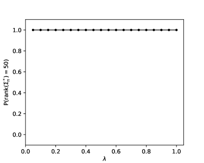
Figure 6: Plot for Claim (v).
In this experiment, we use the linear kernel $k_{\Sigma}(x,x^{\prime})=x^{T}\Sigma x^{\prime}$. We sample $X\sim\mathsf{N}(0,I)$ and $Y=X_{1}+X_{2}+X_{3}+\epsilon$, where $\epsilon\sim N(0,\sigma^{2})$ with $\sigma=0.1$. Here, we set $n=300$ and $p=50$.
The solution is always full rank: ${\rm rank}(\Sigma_{n}^{*})=50$ for every $\lambda>0$ in the $100$ repeated experiments.

References

- [ACHL19] Sanjeev Arora, Nadav Cohen, Wei Hu, and Yuping Luo, Implicit regularization in deep matrix factorization, Advances in Neural Information Processing Systems 32 (2019).
- [Aro50] Nachman Aronszajn, Theory of reproducing kernels, Transactions of the American Mathematical Society 68 (1950), no. 3, 337–404.
- [Bak73] Charles R Baker, Joint measures and cross-covariance operators, Transactions of the American Mathematical Society 186 (1973), 273–289.
- [Ber97] Dimitri P Bertsekas, Nonlinear programming, Journal of the Operational Research Society 48 (1997), no. 3, 334–334.
- [Bil13] Patrick Billingsley, Convergence of probability measures, John Wiley & Sons, 2013.
- [BM87] Richard J Beckman and Michael D McKay, Monte Carlo estimation under different distributions using the same simulation, Technometrics 29 (1987), no. 2, 153–160.
- [BM88] James V Burke and Jorge J Moré, On the identification of active constraints, SIAM Journal on Numerical Analysis 25 (1988), no. 5, 1197–1211.
- [BM03] Samuel Burer and Renato DC Monteiro, A nonlinear programming algorithm for solving semidefinite programs via low-rank factorization, Mathematical Programming 95 (2003), no. 2, 329–357.
- [CDV07] Andrea Caponnetto and Ernesto De Vito, Optimal rates for the regularized least-squares algorithm, Foundations of Computational Mathematics 7 (2007), 331–368.
- [CFJL18] Emmanuel Candes, Yingying Fan, Lucas Janson, and Jinchi Lv, Panning for gold: ‘Model-X’ knockoffs for high dimensional controlled variable selection, Journal of the Royal Statistical Society Series B: Statistical Methodology 80 (2018), no. 3, 551–577.
- [CL02] R Dennis Cook and Bing Li, Dimension reduction for conditional mean in regression, The Annals of Statistics 30 (2002), no. 2, 455–474.
- [CN94] R Dennis Cook and Christopher J Nachtsheim, Reweighting to achieve elliptically contoured covariates in regression, Journal of the American Statistical Association (1994), 592–599.
- [Coo98] R Dennis Cook, Regression graphics, John Wiley & Sons, 1998.
- [Coo04] , Testing predictor contributions in sufficient dimension reduction, The Annals of Statistics 32 (2004), no. 3, 1062–1092.
- [CS02] Felipe Cucker and Steve Smale, On the mathematical foundations of learning, Bulletin of the American mathematical society 39 (2002), no. 1, 1–49.
- [CVBM02] Olivier Chapelle, Vladimir Vapnik, Olivier Bousquet, and Sayan Mukherjee, Choosing multiple parameters for support vector machines, Machine learning 46 (2002), 131–159.
- [DDL14] Aris Daniilidis, Dmitriy Drusvyatskiy, and Adrian S Lewis, Orthogonal invariance and identifiability, SIAM Journal on Matrix Analysis and Applications 35 (2014), no. 2, 580–598.
- [DKS21] Zhen Dai, Mina Karzand, and Nathan Srebro, Representation costs of linear neural networks: Analysis and design, Advances in Neural Information Processing Systems 34 (2021), 26884–26896.
- [DL14] Dmitriy Drusvyatskiy and Adrian S Lewis, Optimality, identifiability, and sensitivity, Mathematical Programming 147 (2014), no. 1-2, 467–498.
- [Dru13] Dmitriy Drusvyatskiy, Slope and geometry in variational mathematics.
- [Dun87] John C Dunn, On the convergence of projected gradient processes to singular critical points, Journal of Optimization Theory and Applications 55 (1987), 203–216.
- [FBG07] Kenji Fukumizu, Francis R Bach, and Arthur Gretton, Statistical consistency of kernel canonical correlation analysis., Journal of Machine Learning Research 8 (2007), no. 2.
- [FBJ04] Kenji Fukumizu, Francis R Bach, and Michael I Jordan, Dimensionality reduction for supervised learning with reproducing kernel Hilbert spaces, Journal of Machine Learning Research 5 (2004), no. Jan, 73–99.
- [FBJ09] , Kernel dimension reduction in regression, The Annals of Statistics 37 (2009), no. 4, 1871–1905.
- [FGB05] Kenji Fukumizu, Arthur Gretton, and Francis Bach, Statistical convergence of kernel cca, Advances in Neural Information Processing Systems 18 (2005).
- [FH01] Jianqing Fan and Li-Shan Huang, Goodness-of-fit tests for parametric regression models, Journal of the American Statistical Association 96 (2001), no. 454, 640–652.
- [FMP18] Jalal Fadili, Jérôme Malick, and Gabriel Peyré, Sensitivity analysis for mirror-stratifiable convex functions, SIAM Journal on Optimization 28 (2018), no. 4, 2975–3000.
- [GA11] Mehmet Gönen and Ethem Alpaydın, Multiple kernel learning algorithms, The Journal of Machine Learning Research 12 (2011), 2211–2268.
- [GBSS05] Arthur Gretton, Olivier Bousquet, Alex Smola, and Bernhard Schölkopf, Measuring statistical dependence with Hilbert-Schmidt norms, International conference on algorithmic learning theory, Springer, 2005, pp. 63–77.
- [GWB+17] Suriya Gunasekar, Blake E Woodworth, Srinadh Bhojanapalli, Behnam Neyshabur, and Nati Srebro, Implicit regularization in matrix factorization, Advances in neural information processing systems 30 (2017).
- [GWBV02] Isabelle Guyon, Jason Weston, Stephen Barnhill, and Vladimir Vapnik, Gene selection for cancer classification using support vector machines, Machine learning 46 (2002), 389–422.
- [HJ12] Roger A Horn and Charles R Johnson, Matrix analysis, Cambridge university press, 2012.
- [HJPS01] Marian Hristache, Anatoli Juditsky, Jorg Polzehl, and Vladimir Spokoiny, Structure adaptive approach for dimension reduction, The Annals of Statistics (2001), 1537–1566.
- [HL04] Warren L Hare and Adrian S Lewis, Identifying active constraints via partial smoothness and prox-regularity, Journal of Convex Analysis 11 (2004), no. 2, 251–266.
- [HL07] , Identifying active manifolds, Algorithmic Operations Research 2 (2007), no. 2, 75–82.
- [HTF09] Trevor Hastie, Robert Tibshirani, and Jerome H Friedman, The elements of statistical learning: data mining, inference, and prediction, vol. 2, Springer, 2009.
- [HTW15] Trevor Hastie, Robert Tibshirani, and Martin Wainwright, Statistical learning with sparsity: the lasso and generalizations, CRC press, 2015.
- [HUM12] Jean-Baptiste Hiriart-Urruty and Jérôme Malick, A fresh variational-analysis look at the positive semidefinite matrices world, Journal of Optimization Theory and Applications 153 (2012), 551–577.
- [JDST20] Ziwei Ji, Miroslav Dudík, Robert E Schapire, and Matus Telgarsky, Gradient descent follows the regularization path for general losses, Conference on Learning Theory, PMLR, 2020, pp. 2109–2136.
- [JLR21] Michael I Jordan, Keli Liu, and Feng Ruan, On the self-penalization phenomenon in feature selection, arXiv preprint arXiv:2110.05852 (2021).
- [KG00] Vladimir Koltchinskii and Evarist Giné, Random matrix approximation of spectra of integral operators, Bernoulli (2000), 113–167.
- [KW70] George S Kimeldorf and Grace Wahba, A correspondence between bayesian estimation on stochastic processes and smoothing by splines, The Annals of Mathematical Statistics 41 (1970), no. 2, 495–502.
- [LCB+04] Gert RG Lanckriet, Nello Cristianini, Peter Bartlett, Laurent El Ghaoui, and Michael I Jordan, Learning the kernel matrix with semidefinite programming, Journal of Machine learning research 5 (2004), no. Jan, 27–72.
- [Lew02] Adrian S Lewis, Active sets, nonsmoothness, and sensitivity, SIAM Journal on Optimization 13 (2002), no. 3, 702–725.
- [Li91] Ker-Chau Li, Sliced inverse regression for dimension reduction, Journal of the American Statistical Association 86 (1991), no. 414, 316–327.
- [LLL21] Zhiyuan Li, Yuping Luo, and Kaifeng Lyu, Towards resolving the implicit bias of gradient descent for matrix factorization: Greedy low-rank learning, International Conference on Learning Representations, 2021.
- [LLY14] Wei Luo, Bing Li, and Xiangrong Yin, On efficient dimension reduction with respect to a statistical functional of interest, The Annals of Statistics (2014), 382–412.
- [LMZ18] Yuanzhi Li, Tengyu Ma, and Hongyang Zhang, Algorithmic regularization in over-parameterized matrix sensing and neural networks with quadratic activations, Conference On Learning Theory, PMLR, 2018, pp. 2–47.
- [LZC05] Bing Li, Hongyuan Zha, and Francesca Chiaromonte, Contour regression: A general approach to dimension reduction, The Annals of Statistics (2005), 1580–1616.
- [LZL18] Qian Lin, Zhigen Zhao, and Jun S Liu, On consistency and sparsity for sliced inverse regression in high dimensions, The Annals of Statistics 46 (2018), no. 2, 580–610.
- [New91] Whitney K Newey, Uniform convergence in probability and stochastic equicontinuity, Econometrica: Journal of the Econometric Society (1991), 1161–1167.
- [POW23] Suzanna Parkinson, Greg Ongie, and Rebecca Willett, Linear neural network layers promote learning single-and multiple-index models, arXiv preprint arXiv:2305.15598 (2023).
- [RBPB22] Adityanarayanan Radhakrishnan, Daniel Beaglehole, Parthe Pandit, and Mikhail Belkin, Feature learning in neural networks and kernel machines that recursively learn features, arXiv preprint arXiv:2212.13881 (2022).
- [RR07] Ali Rahimi and Benjamin Recht, Random features for large-scale kernel machines, Advances in neural information processing systems 20 (2007).
- [Sam93] Alexander M Samarov, Exploring regression structure using nonparametric functional estimation, Journal of the American Statistical Association 88 (1993), no. 423, 836–847.
- [Sch38] Isaac J Schoenberg, Metric spaces and completely monotone functions, Annals of Mathematics (1938), 811–841.
- [Sch42] , Positive definite functions on spheres, Duke Mathematical Journal (1942).
- [SDBR14] Huibin Shen, Kai Dührkop, Sebastian Böcker, and Juho Rousu, Metabolite identification through multiple kernel learning on fragmentation trees, Bioinformatics 30 (2014), no. 12, i157–i164.
- [SFL11] Bharath K Sriperumbudur, Kenji Fukumizu, and Gert RG Lanckriet, Universality, characteristic kernels and RKHS embedding of measures., Journal of Machine Learning Research 12 (2011), no. 7.
- [SHS01] Bernhard Schölkopf, Ralf Herbrich, and Alex J Smola, A generalized representer theorem, International conference on computational learning theory, Springer, 2001, pp. 416–426.
- [SMCB16] Yauheniya Shynkevich, T Martin McGinnity, Sonya A Coleman, and Ammar Belatreche, Forecasting movements of health-care stock prices based on different categories of news articles using multiple kernel learning, Decision Support Systems 85 (2016), 74–83.
- [SNYB19] Oliver Stromann, Andrea Nascetti, Osama Yousif, and Yifang Ban, Dimensionality reduction and feature selection for object-based land cover classification based on Sentinel-1 and Sentinel-2 time series using Google Earth Engine, Remote Sensing 12 (2019), no. 1, 76.
- [SRJ04] Nathan Srebro, Jason Rennie, and Tommi Jaakkola, Maximum-margin matrix factorization, Advances in neural information processing systems 17 (2004).
- [SS90] Gilbert W Stewart and Ji-guang Sun, Matrix perturbation theory.
- [SVV+18] Hector Sanz, Clarissa Valim, Esteban Vegas, Josep M Oller, and Ferran Reverter, SVM-RFE: selection and visualization of the most relevant features through non-linear kernels, BMC bioinformatics 19 (2018), no. 1, 1–18.
- [SWNW03] Thomas J Santner, Brian J Williams, William I Notz, and Brain J Williams, The design and analysis of computer experiments, vol. 1, Springer, 2003.
- [TQP22] Ting Tao, Yitian Qian, and Shaohua Pan, Column -norm regularized factorization model of low-rank matrix recovery and its computation, SIAM Journal on Optimization 32 (2022), no. 2, 959–988.
- [TVS23] Nadav Timor, Gal Vardi, and Ohad Shamir, Implicit regularization towards rank minimization in relu networks, International Conference on Algorithmic Learning Theory, PMLR, 2023, pp. 1429–1459.
- [VdV00] Aad W Van der Vaart, Asymptotic statistics, vol. 3, Cambridge university press, 2000.
- [Wah90] Grace Wahba, Spline models for observational data, SIAM, 1990.
- [Wai19] Martin J Wainwright, High-dimensional statistics: A non-asymptotic viewpoint, vol. 48, Cambridge University Press, 2019.
- [Wen04] Holger Wendland, Scattered data approximation, vol. 17, Cambridge university press, 2004.
- [WMC+00] Jason Weston, Sayan Mukherjee, Olivier Chapelle, Massimiliano Pontil, Tomaso Poggio, and Vladimir Vapnik, Feature selection for SVMs, Advances in neural information processing systems 13 (2000).
- [Wri93] Stephen J Wright, Identifiable surfaces in constrained optimization, SIAM Journal on Control and Optimization 31 (1993), no. 4, 1063–1079.
- [XTLZ02] Yingcun Xia, Howell Tong, Wai Keung Li, and Li-Xing Zhu, An adaptive estimation of dimension reduction space, Journal of the Royal Statistical Society Series B: Statistical Methodology 64 (2002), no. 3, 363–410.
- [YDS16] Zhou Yu, Yuexiao Dong, and Jun Shao, On marginal sliced inverse regression for ultrahigh dimensional model-free feature selection, The Annals of Statistics 44 (2016), no. 6, 2594–2623.
- [YL11] Xiangrong Yin and Bing Li, Sufficient dimension reduction based on an ensemble of minimum average variance estimators, The Annals of Statistics (2011), 3392–3416.
- [Zen08] Peng Zeng, Determining the dimension of the central subspace and central mean subspace, Biometrika 95 (2008), no. 2, 469–479.
- [ZO07] Alexander Zien and Cheng Soon Ong, Multiclass multiple kernel learning, Proceedings of the 24th international conference on Machine learning, 2007, pp. 1191–1198.
- [ZZ06] Yu Zhu and Peng Zeng, Fourier methods for estimating the central subspace and the central mean subspace in regression, Journal of the American Statistical Association 101 (2006), no. 476, 1638–1651.