Simultaneous Nonparametric Inference of M-regression under Complex Temporal Dynamics

Abstract

The paper considers simultaneous nonparametric inference for a wide class of M-regression models with time-varying coefficients. The covariates and errors of the regression model are tackled as a general class of piece-wise locally stationary time series and are allowed to be cross-dependent. We introduce an integration technique to study the M-estimators, whose limiting properties are disclosed using Bahadur representation and Gaussian approximation theory. Facilitated by a self-convolved bootstrap proposed in this paper, we introduce a unified framework to conduct general classes of Exact Function Tests, Lack-of-fit Tests, and Qualitative Tests for the time-varying coefficient M-regression under complex temporal dynamics. As an application, our method is applied to studying the anthropogenic warming trend and time-varying structures of the ENSO effect using global climate data from 1882 to 2005.

Keywords: Cumulative regression function, piece-wise locally stationary time series, method of aggregation, self-convolved bootstrap

1 Introduction

Over the past few years, there has been an increasing necessity to account for temporal nonstationarity in statistical analysis. For instance, financial returns are frequently non-stationary (Francq and Sucarrat,, 2023), and the stock market underwent considerable instability during the Covid-19 pandemic. Climate change also becomes progressively unpredictable with extreme weather happening globally with greater intensity (Ebi et al.,, 2021). In the field of physiology, complex oscillatory signals are usually contaminated by non-stationary noise and may change abruptly in frequency or amplitude (Wu and Zhou,, 2023). See also Dahlhaus, (2012); Dahlhaus et al., (2019); Zhou, (2013); Nason, (2013); Vogt, (2012); Dette et al., (2011); Kreiss and Paparoditis, (2014) among others for the recent statistics literature on non-stationary time series analysis. As deviations from temporal homogeneity become more pronounced, static statistical models may be inadequate in accurately capturing the dynamic features of the data. In the context of regression analysis, one of the successful generalizations is to use the varying-coefficient model (Fan and Zhang,, 1999; Hastie and Tibshirani,, 1993), which allows one to choose regression coefficients as a smooth function of time. As has been extensively discussed in the previous literature, the varying-coefficient model is capable of capturing the non-constant relationship between the predictor variables and the response; see, for instance, Fan and Zhang, (2000); Hoover et al., (1998); Zhou and Wu, (2010); Zhang and Wu, (2012); Wu and Zhou, (2017), among many others. In this paper, we shall consider the following time-varying M-regression (Huber,, 1964, 1973) model for non-stationary time series:

$$y_{i}={\bf x}_{i}^{\top}\mbox{\boldmath$\beta$}_{i}+e_{i},\quad i=1,2,\cdots,n,$$ (1)

where $\{{\bf x}_{i}=(x_{i1},\cdots,x_{ip})^{\top}\}_{i=1}^{n}$ is a $p$-dimensional non-stationary covariate (or predictor) process, $\{e_{i}\}_{i=1}^{n}$ is a non-stationary error process satisfying $\mathbb{E}(\psi(e_{i})|{\bf x}_{i},{\bf x}_{i-1},\cdots,{\bf x}_{1})=0$ almost surely with $\psi(\cdot)$ being the left derivative of a convex function $\rho(\cdot)$ , and $\mbox{\boldmath$\beta$}_{i}=\mbox{\boldmath$\beta$}(t_{i})=$ $(\beta_{0}(t_{i}),\cdots,\beta_{p-1}(t_{i}))^{\top}$ is the coefficient $\mbox{\boldmath$\beta$}(t)$ evaluated at time $t_{i}=i/n$. We study model (1) in a general framework where $\{{\bf x}_{i}\}$ and $\{e_{i}\}$ belong to a general class of non-stationary time series models with both smoothly and abruptly time-varying dynamics. The detailed assumptions of the model are deferred to Section 7. Observe that (1) includes a wide range of regression models with flexible choices of $\rho(\cdot)$. Prominent examples include the least square regression with $\rho(x)=x^{2}$, the quantile regression with $\rho(x)=\tau x^{+}+(1-\tau)(-x)^{+}$, $\tau\in(0,1)$, $x^{+}=\max(x,0)$, the $L^{q}$ regression with $\rho(x)=|x|^{q}$, $q>0$, the expectile regression with $\rho(x)=|I(x\leq 0)-\alpha|x^{2}$, $\alpha\in(0,1)$, and Huber’s robust regression with $\rho(x)=x^{2}I(|x|\leq\varsigma)/2+(\varsigma|x|-\varsigma^{2}/2)I(|x|>\varsigma)$, $\varsigma>0$.

The purpose of this article is to give a unified framework for nonparametric inference of the non-stationary time series regression model (1). In particular, regarding the coefficient function $\mbox{\boldmath$\beta$}(t)$, we are interested in conducting three types of hypothesis tests: Exact Function Tests, Lack-of-fit Tests, and Qualitative Tests. The first type, Exact Function Test (EFT), takes the form of $H_{0}:\mbox{\boldmath$\beta$}(t)=\mbox{\boldmath$\beta$}_{0}(t)$ for some specific $\mbox{\boldmath$\beta$}_{0}(t)$, which, for example, enables one to perform the conventional significance testing by letting $\mbox{\boldmath$\beta$}_{0}(t)=\mathbf{0}$. Secondly, the Lack-of-fit Test (LOFT), also referred to as diagnostic test (Stute,, 1997), tackles the circumstance where the null hypothesis is a parametric family while the alternative remains nonparametric (He and Zhu,, 2003). This includes, but is not limited to, the tests of constancy and linearity of the function versus a general smooth alternative. Apart from the aforementioned two types of tests, statisticians may also want to check qualitative beliefs on functions where the null hypothesis is a relatively general nonparametric class of functions (Komarova and Hidalgo,, 2020). For example, many economic models use certain shape restrictions (e.g., monotonicity, convexity) as plausible restrictions (Fang and Seo,, 2021). While those prespecified qualitative shape assumptions facilitate the inference and enhance performance (Friedman and Tibshirani,, 1984), wrong conclusions can be drawn when these assumptions are not satisfied. The necessity to conduct Qualitative Tests (QT), therefore, becomes axiomatic. In the present work, we address the tests by developing two novel tools. First, in lieu of directly focusing on the inference of $\mbox{\boldmath$\beta$}(t)$, we implement an integration technique, investigating the cumulative regression function (CRF)

$$\Lambda(t)=(\Lambda_{1}(t),\cdots,\Lambda_{p}(t))^{\top}=\int_{0}^{t}\mbox{\boldmath$\beta$}(s)\,ds,\quad 0\leq t\leq 1,$$ (2)

and we propose in Section 2 to obtain its estimator by partial sums of local M-estimators of $\mbox{\boldmath$\beta$}(t)$. There are two main reasons for considering $\Lambda(t)$ instead of $\mbox{\boldmath$\beta$}(t)$ in the inference. First, as is suggested in Theorem 1, the CRF can be estimated at a parametric rate of $\sqrt{n}$. Such merits of getting $\sqrt{n}$ convergence via integration have also been demonstrated by Hall and Marron, (1987) and Bickel and Ritov, (1988) when estimating integrated squared density derivatives, and by Huang and Fan, (1999) for nonparametric estimation of quadratic regression functionals. Recently, Mies, (2023) employed the method for estimating parameters of locally stationary time series, leading to a $\sqrt{n}$ functional central limit theorem. Although the results in the existing literature have gradually adapted from the i.i.d. case to a broader non-stationary time series setup, they do not apply to the M-regression setting. To our knowledge, no comparable research has been conducted on uniform nonparametric inference of the CRF under the time-varying M-regression framework. The second reason, possibly more salient, pertains to the complexity of the temporal dynamics considered. Specifically, it is difficult to theoretically investigate and consistently estimate the (asymptotic) distributional behavior of the M-estimators around the time points where ${\bf x}_{i}$ and/or $e_{i}$ experience abrupt changes in their underlying data-generating mechanisms. As a result, directly inferring the M-estimators of $\mbox{\boldmath$\beta$}(\cdot)$ simultaneously over time becomes challenging. Nevertheless, we discover in this work that aggregated M-estimators of the CRF converge to a Gaussian process with a complex covariance structure uniformly over time under mild conditions. Furthermore, the uniform temporal behavior of the latter aggregated M-estimators can be well approximated by a simple and unified bootstrap procedure. Consequently, it is simpler and more accurate to make simultaneous inferences of $\Lambda(\cdot)$ than $\mbox{\boldmath$\beta$}(\cdot)$ under complex temporal dynamics. As far as we know, there is no previous literature utilizing the method of integration or aggregation to alleviate the effect of complex dependence and heteroscedasticity in regression analysis.

As a second contribution, we propose in this paper a self-convolved bootstrap procedure, which shares a unified construction among a broad class of M-estimators and hypothesis tests. It is proven to be consistent under non-stationary temporal dependence and predictor-error dependence. The idea of bootstrap has been widely accepted for the inference of nonparametric regression (Hardle and Marron,, 1991; Stute et al., 1998a, ; Diciccio and Romano,, 1988). In particular, the bootstrap approximation of an unknown population can usually accelerate the convergence and circumvent the problem of directly estimating the limiting process, as suggested in Zhou and Wu, (2010). In the context of time series nonparametric M-regression, however, so far there exist no valid bootstrap methods for its simultaneous inference when the underlying data generating mechanism contains possible jumps. The most related work can be found in Wu and Zhou, (2017) where the authors proposed a bootstrap procedure for time-varying coefficient quantile regression with smoothly time-varying dynamics. The main difficulty in designing bootstrap methods under complex temporal dynamics, again, lies in the inconsistency in estimating various key quantities around the jump points. Another challenge that arises in the bootstrap inference of M-regression is the need to estimate a density-like function which requires the delicate choice of a tuning parameter (Koenker,, 2005). For instance, in quantile regression where $\rho(x)=\tau x^{+}+(1-\tau)(-x)^{+}$, the asymptotic behavior of local estimates of $\mbox{\boldmath$\beta$}(\cdot)$ is involved with a density-type quantity $\Sigma(\cdot)$ (Wu and Zhou,, 2017). A tuning parameter is needed to estimate $\Sigma(\cdot)$ nonparametrically. In moderate samples, the quality of the bootstrap inference depends on the estimation accuracy of $\Sigma(\cdot)$, which substantially relies on the nontrivial task of selecting the aforementioned tuning parameter.

As its name implies, the proposed self-convolved bootstrap method only necessitates the convolution of the M-estimators with i.i.d. auxiliary standard normal variables, which eliminates the need for additional computation. In particular, there is no need to estimate the aforementioned density-like quantities. The construction principle applies uniformly to a wide class of M-estimators and hence saves lots of effort when conducting inference based on various types of estimators simultaneously. Following the integration technique, we will show that the easy-to-implement bootstrap mimics the probabilistic behavior of the M-estimators of the CRF consistently. Mutually enhancing one another, the integration technique and self-convolved bootstrap address different types of tests using a unified asymptotic result, which venture into a new avenue compared to the conventional methods.

Historically in the context of regression, much literature has focused on the Lack-of-fit Test on the regression mean function, serving as a key component in model checking. One popular methodology is to obtain the parametric and nonparametric curve estimates separately, followed by computing the discrepancies between them as a natural test statistic. The representative results can be found in Hardle and Mammen, (1993) and Hong and White, (1995). Similarly, Chen and Hong, (2012) proposed a generalized Hausman test for checking parameter stability in time series models, which was developed under a $L_{2}$-regression framework and applicable to stationary covariates and errors. Alternatively, another distinguished direction is to study the empirical process based on residuals; see Stute, (1997); Stute et al., 1998b ; Koul and Stute, (1999). Recently, Mies, (2023) utilized the integration technique for change-point detection of local parameters. In comparison, our current work is based on a new self-convolved bootstrap technique and applies to a broader range of tests and a more general M-regression setting. Different from the Lack-of-fit Test where the null hypothesis forms a parametric family, qualitative hypotheses often include shape constraints that are more complicated to deal with. To test the monotonicity of a regression curve, Bowman et al., (1998) exploited Silverman, (1981)’s idea of critical bandwidth. Gijbels et al., (2000) and Ghosal et al., (2000) formulated monotonicity of the regression curve as the concordance of $X$ and $Y$. As a distinctive approach, Durot, (2003) transformed the test of monotonicity into testing whether the integral coincides with its least concave majorant. A localized version of the test was later elaborated by Akakpo et al., (2014), which demonstrated better power performance due to replications of the test on subintervals. Other contributions in nonparametric qualitative tests include Hall and Heckman, (2000), I. Gijbels and Verhasselt, (2017); Komarova and Hidalgo, (2020) and Fang and Seo, (2021), among others.

The rest of the paper is structured as follows. Section 2 introduces the piece-wise locally stationary time series, dependence measures and local linear M-estimators. The estimator for the CRF is proposed, along with its asymptotic results stated in Theorem 1. Section 3 presents the construction of the self-convolved bootstrap. In Section 4, three types of hypothesis tests are discussed separately, where detailed algorithms and their asymptotic behaviors are provided. The finite-sample performance of our methodology is demonstrated in Section 5, followed by an empirical illustration using global climate data in Section 6. Regularity conditions of the model and auxiliary theoretical results about Bahadur representation are given in Section 7. Theoretical proofs are provided in the supplementary material.

2 The Cumulative Regression Function

We start by introducing some notations. For an $m$-dimensional (random) vector $\boldsymbol{v}=(v_{1},\cdots,v_{m}),m\geq 1$, let $|v|$ be the Euclidean norm and $|v|_{\infty}:=\max_{i=1}^{m}|v_{i}|$. Let $I\{\cdot\}$ be the indicator function and we denote the weak convergence by $\Rightarrow$.

2.1 Preliminary: non-stationary time series models

The following piece-wise locally stationary (PLS) time series models (Zhou,, 2013) are used to describe the complex temporal dynamics of the covariates and errors. For a sequence of i.i.d. random variables $\{\eta_{i}\}_{i=-\infty}^{\infty}$, let $\{\eta^{\prime}_{i}\}_{i=-\infty}^{\infty}$ be an i.i.d. copy. Define $\mathcal{F}_{i}=(\cdots,\eta_{i-1},\eta_{i})$, and $\mathcal{F}_{i}^{*}=({\cal F}_{-1},\eta_{0}^{\prime},\eta_{1},\cdots,\eta_{i})$.

Definition 1.

We say that $\{{\bf Z}_{i}\}$ is a $d$-dimensional piece-wise locally stationary time series with $r$ break points and filtration $\{\mathcal{F}_{i}\}$ if

$${\bf Z}_{i}=\sum_{j=0}^{r}G_{j}(i/n,\mathcal{F}_{i})I\{i/n\in(w_{j},w_{j+1}]\},\quad i=1,2,\cdots,n,$$ (3)

where $0=w_{0}<w_{1}<\cdots<w_{r}<w_{r+1}=1$, and $G_{j}:$ $[w_{j},w_{j+1}]\times\mathbb{R}^{\mathbb{Z}}\rightarrow\mathbb{R}^{d}$, $j=0,1,\cdots,r$.

The breakpoints $w_{1},\cdots,w_{r}$ are assumed to be fixed but unknown, and the number of breaks $r$ is assumed to be bounded. Note that the data-generating mechanism of $\{{\bf Z}_{i}\}$ can change abruptly from $G_{j-1}(\cdot)$ to $G_{j}(\cdot)$ at the breakpoint $w_{j}$, and it evolves smoothly between adjacent breakpoints. Let $\zeta_{i}$ be the index $j$ such that $i/n\in(w_{j},w_{j+1}]$. Then (3) is equivalent to ${\bf Z}_{i}=G_{\zeta_{i}}(i/n,\mathcal{F}_{i})$. For $q>0$ and $i\geq 0$, we define the dependence measures

$$\delta_{{\bf Z}}(i,q)=\max_{0\leq j\leq r}\sup_{w_{j}\leq t\leq w_{j+1}}\|G_{j}({t,\cal F}_{i})-G_{j}(t,\mathcal{F}_{i}^{*})\|_{q},$$ (4)

where $\|\cdot\|_{q}=\{\mathbb{E}[|\cdot|^{q}]\}^{1/q}$ is the ${\cal L}^{q}$ norm. Write $\|\cdot\|:=\|\cdot\|_{2}$. Let $\delta_{{\bf Z}}(i,q)=0$ if $i<0$.

Here we consider filtrations $\mathcal{F}_{i}=(\cdots,\eta_{i-1},\eta_{i})$ and $\mathcal{G}_{i}=(\cdots,\tau_{i-1},\tau_{i})$, where $\{\eta_{i}\}_{i=-\infty}^{\infty}$ and $\{\tau_{i}\}_{i=-\infty}^{\infty}$ are independent. Further assume piece-wise locally stationary time series ${\bf x}_{i}={\bf H}_{\zeta_{i}}(t_{i},\mathcal{G}_{i})$, $e_{i}=G_{\zeta_{i}}(t_{i},\mathcal{F}_{i},\mathcal{G}_{i})$. Observe that ${\bf x}_{i}$ and $e_{i}$ can be dependent. Without loss of generality, assume they share the same $r$ breakpoints $0=w_{0}<\cdots<w_{r}<w_{r+1}=1$.

2.2 Aggregated local estimation of the CRF

Throughout this paper, we assume that the regression function $\mbox{\boldmath$\beta$}(t)\in{\cal C}^{2}[0,1]$. For any $t\in(0,1)$, since $\mbox{\boldmath$\beta$}(s)\approx\mbox{\boldmath$\beta$}(t)+\mbox{\boldmath$\beta$}^{\prime}(t)(s-t)$ in a small neighborhood of $t$, we define the preliminary local linear M-estimates of $\mbox{\boldmath$\beta$}(t)$ and $\mbox{\boldmath$\beta$}^{\prime}(t)$ by

$$\tilde{\mbox{\boldmath$\beta$}}_{b_{n}}(t):=\left(\begin{array}[]{c}\hat{\mbox{\boldmath$\beta$}}_{b_{n}}(t)\\ \hat{\mbox{\boldmath$\beta$}}_{b_{n}}^{\prime}(t)\end{array}\right)=\mathop{\mbox{argmin}}_{\mbox{\boldmath$b$}_{0},\mbox{\boldmath$b$}_{1}\in\mathbb{R}^{p}}\sum_{i=1}^{n}\rho(y_{i}-{\bf x}_{i}^{\top}\mbox{\boldmath$b$}_{0}-{\bf x}_{i}^{\top}\mbox{\boldmath$b$}_{1}(t_{i}-t))K((t_{i}-t)/b_{n}),$$ (7)

where $t_{i}=i/n$, $b_{n}$ is a bandwidth satisfying $b_{n}\rightarrow 0$, and $\rho(\cdot)$ is a convex loss function with left derivative $\psi(\cdot)$. In this paper, we also assume robustness of the loss functions in the sense that $|\psi(x)-\psi(y)|\leq M_{1}+M_{2}|x-y|$ for $\forall x,y\in\mathbb{R}$ and some positive constants $M_{1},M_{2}$. $K(\cdot)$ is a kernel function satisfying $K\in{\cal K}$ and ${\cal K}$ is collection of symmetric and ${\cal C}^{1}$ density functions with support $[-1,1]$.

Recall the CRF defined in (2), then the regression function $\mbox{\boldmath$\beta$}(\cdot)$ can be retrieved via

$$\mbox{\boldmath$\beta$}(t)=\Lambda^{\prime}(t-)\quad 0<t\leq 1\quad\mbox{and}\quad\mbox{\boldmath$\beta$}(0)=\Lambda^{\prime}(0+),$$

where $\Lambda^{\prime}(t-)$ and $\Lambda^{\prime}(t+)$ represent the left and right derivative of $\Lambda(t)$, respectively.

As is discussed in Section 7, the M-estimator $\hat{\mbox{\boldmath$\beta$}}_{b_{n}}(t)$ obtained in (7) involves a bias term regarding $\mbox{\boldmath$\beta$}^{\prime\prime}(t)$. In order to proceed without estimating $\mbox{\boldmath$\beta$}^{\prime\prime}(t)$, we shall employ a Jackknife bias-corrected estimator denoted as $\check{\mbox{\boldmath$\beta$}}_{b_{n}}(t)$, where

$$\check{\mbox{\boldmath$\beta$}}_{b_{n}}(t):=2\hat{\mbox{\boldmath$\beta$}}_{b_{n}/\sqrt{2}}(t)-\hat{\mbox{\boldmath$\beta$}}_{b_{n}}(t).$$ (8)

The implementation of the bias-correction procedure is asymptotically equivalent to using the second-order kernel $K^{*}(x):=2\sqrt{2}K(\sqrt{2}x)-K(x)$ (Wu and Zhou,, 2017). In this way, the bias of $\check{\mbox{\boldmath$\beta$}}_{b_{n}}(t)$ is asymptotically negligible under mild conditions. We propose to estimate $\Lambda(t)$ via

$$\check{\Lambda}(t_{j})=\sum_{i=1}^{j}\check{\mbox{\boldmath$\beta$}}_{b_{n}}(t_{i})/n,\quad 1\leq j\leq n.$$ (9)

Set $\check{\Lambda}(0)=0$. For any $t\in[0,1]$, let $\check{\Lambda}(t)$ be the linear interpolation of the sequence $\{\check{\Lambda}(t_{j})\}_{j=0}^{n}$. We omit the subscript $b_{n}$ of $\check{\mbox{\boldmath$\beta$}}_{b_{n}}(t)$ hereafter, whenever no confusion caused.

Let $\mathbf{C}$ be a fixed $s\times p$, $s\leq p$ full rank matrix, we are interested in testing the dynamic pattern of $\mbox{\boldmath$\beta$}_{\mathbf{C}}(\cdot):=\mathbf{C}\mbox{\boldmath$\beta$}(\cdot)$, which includes any linear combination of $\{\mbox{\boldmath$\beta$}_{j}(\cdot)\}_{j=0}^{p-1}$. As a result, for the CRF ${\Lambda}_{\mathbf{C}}(t):=\mathbf{C}{\Lambda}(t)$, its estimator can be obtained via $\check{\Lambda}_{\mathbf{C}}(t):=\mathbf{C}\check{\Lambda}(t)$. Based on the Bahadur representation presented in Section 7, the following theorem establishes a $\sqrt{n}$-consistent Gaussian weak convergence result for the proposed integrated M-estimator:

Theorem 1.

Assume that Assumptions (A1)-(A7) in Section 7 hold, $\frac{nb_{n}^{4}}{\log^{8}n}\to\infty$, $n^{c}b_{n}\to 0$ for some positive constant $c$, and let $\Psi_{\mathbf{C}}(t)=(\mathbf{C}\Sigma^{-1}(t)\Psi(t)\Sigma^{-1}(t)\mathbf{C}^{\top})^{\frac{1}{2}}$ with $\Sigma(t)$ and $\Psi(t)$ defined in Section 7. Then we have

$$\left\{\sqrt{n}(\check{\Lambda}_{\mathbf{C}}(t)-\Lambda_{\mathbf{C}}(t))\right\}_{0<t<1}\Rightarrow\left\{\mathbf{U}(t)\right\}_{0<t<1},$$

where $\left\{\mathbf{U}(t)\right\}$ is a mean 0 Gaussian process with $\text{Cov}(\mathbf{U}(t_{1}),\mathbf{U}(t_{2}))=\int_{0}^{\min(t_{1},t_{2})}\Psi_{\mathbf{C}}(t)\Psi_{\mathbf{C}}^{\top}(t)\;dt$.

3 The Self-convolved Bootstrap

The Gaussian process $\mathbf{U}(t)$ expressed in Theorem 1 provides a theoretical foundation for the simultaneous inference of $\Lambda(t)$, but the implementation is still unaccomplished due to its complex covariance structure. To circumvent the problem, we propose a self-convolved bootstrap method to mimic the behavior of the Gaussian process $\mathbf{U}(t)$.

Let $\mu=\int_{-2}^{2}[K^{*}(t-1)+K^{*}(t+1)-2K^{*}(t)]^{2}\;\mathrm{d}t$, $\{R_{i}\}_{i=1}^{n}$ be i.i.d. standard normal random variables independent of $\{\mathbf{x}_{i}\psi(e_{i})\}_{i=1}^{n}$. For a given bandwidth $c_{n}$, define the bootstrap process $\{\tilde{\boldsymbol{\Phi}}_{n}^{o}(t),t\in(0,1)\}$ as the linear interpolation of $\{\boldsymbol{\Phi}_{n,j}^{o}\}$, where

$$\boldsymbol{\Phi}_{n,j}^{o}=\mathbf{C}\sum_{i=\left\lceil 2nc_{n}\right\rceil}^{j}\sqrt{\frac{c_{n}}{\mu}}(\check{\mbox{\boldmath$\beta$}}_{c_{n}}(t_{i}+c_{n})+\check{\mbox{\boldmath$\beta$}}_{c_{n}}(t_{i}-c_{n})-2\check{\mbox{\boldmath$\beta$}}_{c_{n}}(t_{i}))R_{i},\quad j=\left\lceil 2nc_{n}\right\rceil,\cdots,n-\left\lceil 2nc_{n}\right\rceil.$$

The self-convolved bootstrap process $\tilde{\boldsymbol{\Phi}}_{n}^{o}(t)$ only requires the convolution of local M-regression estimates and i.i.d. standard normal random variables $\{R_{i}\}$. The heuristics behind the bootstrap process stems from two fundamental observations. Firstly, the Bahadur representation of $\{\check{\mbox{\boldmath$\beta$}}(t_{i})\}$ in Section 7 suggests that $\check{\mbox{\boldmath$\beta$}}_{c_{n}}(t_{i}+c_{n})+\check{\mbox{\boldmath$\beta$}}_{c_{n}}(t_{i}-c_{n})-2\check{\mbox{\boldmath$\beta$}}_{c_{n}}(t_{i})$ can be expressed as a weighted block sum of $\{\mathbf{x}_{i}\psi(e_{i})\}_{i=1}^{n}$, where we take the second-order difference as a bias-correction technique. Secondly, Zhou, (2013) demonstrated that for a broad range of non-stationary time series, progressive convolutions of their block sums with i.i.d. standard normal random variables can consistently mimic the joint probabilistic behavior of their partial sum processes. Now observe that $\mathbf{U}(t)$ represents the limiting behavior of a weighted partial sum process of $\{\mathbf{x}_{i}\psi(e_{i})\}_{i=1}^{n}$. By leveraging these observations, the self-convolved bootstrap achieves an accurate simulation of the limiting Gaussian process of the CRF and retains a concise form for a broad range of M-estimators, utilizing just a single tuning parameter.

In contrast, it is difficult to make inference of $\mbox{\boldmath$\beta$}(t)$ directly based on $\check{\mbox{\boldmath$\beta$}}_{b_{n}}(t)$, as the density-like quantity involved in the distributional behavior of $\check{\mbox{\boldmath$\beta$}}_{b_{n}}(t)$ is hard to estimate in practice due to possible discontinuities and the no-trivial task of choosing smoothing parameters. As a result, the CRF considered in this paper, combined with the proposed self-convolved bootstrap, enables us to conduct inference more efficiently and accurately.

To quantify the consistency of $\{\tilde{\boldsymbol{\Phi}}_{n}^{o}(t),t\in(0,1)\}$, we derive a direct comparison of the distribution between $\{\boldsymbol{\Phi}_{n,j}^{o}\}_{j=\lceil 2nc_{n}\rceil}^{n-\lceil 2nc_{n}\rceil}$ and $\{\mathbf{U}(t_{j})\}{{}_{j=\lceil 2nc_{n}\rceil}^{n-\lceil 2nc_{n}\rceil}}$ in the following theorem. First, we define the $ns$-dimensional vector $\mathbf{\Theta}^{B}=[(\mathbf{\Theta}_{1}^{B})^{\top},(\mathbf{\Theta}_{2}^{B})^{\top},\cdots,(\mathbf{\Theta}_{n}^{B})^{\top}]$ with

$$\mathbf{\Theta}_{j}^{B}:=\left\{\begin{array}[]{ll}\boldsymbol{\Phi}_{n,\left\lceil 2nc_{n}\right\rceil}^{o}&\text{ if }j\leq\left\lceil 2nc_{n}\right\rceil\\ \boldsymbol{\Phi}_{n,j}^{o}&\text{ if }\left\lceil 2nc_{n}\right\rceil<j\leq n-\left\lceil 2nc_{n}\right\rceil\\ \boldsymbol{\Phi}_{n,n-\left\lceil 2nc_{n}\right\rceil}^{o}&\text{ if }n-\left\lceil 2nc_{n}\right\rceil<j\leq n\end{array}\right.,$$

and similarly define the $ns$-dimensional vector $\mathbf{U}=[(\mathbf{U}_{1})^{\top},(\mathbf{U}_{2})^{\top},\cdots,(\mathbf{U}_{n})^{\top}]$ with

$$\mathbf{U}_{i}:=\left\{\begin{array}[]{ll}\mathbf{U}(t_{\left\lceil 2nc_{n}\right\rceil})&\text{ if }i\leq\left\lceil 2nc_{n}\right\rceil\\ \mathbf{U}(t_{i})&\text{ if }\left\lceil 2nc_{n}\right\rceil<i\leq n-\left\lceil 2nc_{n}\right\rceil\\ \mathbf{U}(t_{n-\left\lceil 2nc_{n}\right\rceil})&\text{ if }n-\left\lceil 2nc_{n}\right\rceil<i\leq n.\end{array}\right.$$

Recall $\mathbf{U}(t)$ is defined in Theorem 1. Furthermore, we define

$$\Delta:=\max_{1\leq i,j\leq ns}\left|\left[\operatorname{Cov}\left(\mathbf{U}\right)-\operatorname{Cov}(\mathbf{\Theta}^{B}\mid\{\mathbf{x}_{k}\psi(e_{k})\}_{k=1}^{n})\right]_{ij}\right|$$

as a measure of the difference in covariance structure between the bootstrapped process and the limiting Gaussian process.

Theorem 2.

Suppose conditions (A1)-(A7) in Section 7 hold, $\frac{nc_{n}^{4}}{\log^{8}n}\to\infty$, and $nc_{n}^{5}\to 0$, then we have $\Delta=O_{\mathbb{P}}(\sqrt{c_{n}}+nc_{n}^{5})$. Define the sequence of events $A_{n}=\{\Delta\leq(\sqrt{c_{n}}+nc_{n}^{5})h_{n}\}$ where $h_{n}>0$ is a sequence diverging at an arbitrarily slow rate. Then $\mathbb{P}(A_{n})=1-o(1)$. On the event $A_{n}$, for $\delta\in(0,1)$, we have

$$\sup_{|x|>d_{n,p}^{\circ}}\left|\mathbb{P}\left(\max_{\lceil 2nc_{n}\rceil\leq i\leq n-\lceil 2nc_{n}\rceil}|\mathbf{U}(t_{i})|_{\infty}\leq x\right)-\mathbb{P}\left(\max_{\lceil 2nc_{n}\rceil\leq i\leq n-\lceil 2nc_{n}\rceil}|\boldsymbol{\Phi}_{n,i}^{o}|_{\infty}\leq x\mid\{\mathbf{x}_{i}\psi(e_{i})\}_{i=1}^{n}\right)\right|$$ (10)

$$\lesssim \left((\sqrt{c_{n}}+nc_{n}^{5})h_{n}\right)^{1/3}(\log(n))^{1+4\delta/3}+\dfrac{1}{n(\log(n))^{1/2}},$$

where $d_{n,p}^{\circ}=C\left[\left((\sqrt{c_{n}}+nc_{n}^{5})h_{n}\right)^{1/3}\log^{\delta/3}(n)+\log^{-\delta}(n)\right]$ with some finite constant $C$ that does not depend on $n$.

Remark 1.

Theorem 2 guarantees that the conditional behavior of the bootstrap process consistently mimics the distribution of the limiting process ${\bf U}(t)$ in ${\cal L}_{\infty}$ norm. The restricted range $|x|>d_{n,p}^{\circ}$ is to make the Gaussian approximation valid under the circumstance that the variances of $\boldsymbol{\Phi}_{n,i}^{o}$ have no lower bounds. Note that $d_{n,p}^{\circ}$ and the upper bound in (10) converge to $0$ as $n\to\infty$. Accordingly, for a given $\alpha$ and when $n$ is sufficiently large, $d_{n,p}^{\circ}$ will be dominated by the $(1-\alpha)$-th percentile of $\max_{\lceil 2nc_{n}\rceil\leq i\leq n-\lceil 2nc_{n}\rceil}|\boldsymbol{\Phi}_{n,i}^{o}|_{\infty}$, thereby ensuring that the results in Theorem 2 asymptotically validate the bootstrap procedure. Furthermore, under the conditions of Theorem 2, $c_{n}$ converges to $0$, hence the consistency of the bootstrap $\tilde{\boldsymbol{\Phi}}_{n}^{o}(t)$ demonstrated on $[2c_{n},1-2c_{n}]$ is asymptotically uniform on $t\in(0,1)$.

4 Applications to Hypothesis Testing

In principle, hypotheses regarding the regression function $\mbox{\boldmath$\beta$}(t)$ can be expressed equivalently in terms of the CRF $\Lambda(t)$. In this Section, we shall explore the application of the CRF and the self-convolved bootstrap to three general classes of hypothesis tests of the M-regression: Exact Function Tests (EFT), Lack-of-fit Tests (LOFT), and Qualitative Tests (QT).

4.1 Exact Function Test

The Exact Function Test (EFT) amounts to testing the null hypothesis $H_{0}:\mbox{\boldmath$\beta$}_{\mathbf{C}}(t)=f(t),t\in(0,1)$, which can be further reformulated as $H_{0}:\Lambda_{\mathbf{C}}(t)=\int_{0}^{t}f(s)\;ds$, where $f(\cdot)$ is a known function. Define

$$T_{e}:=\sup_{t\in(0,1)}\sqrt{n}\left|\check{\Lambda}_{\mathbf{C}}(t)-\int_{0}^{t}f(s)\;ds\right|_{\infty}.$$ (11)

For any prespecified level $\alpha$, our goal is to find the critical value $q_{\alpha}$, such that $\mathbb{P}\left(T_{e}>q_{\alpha}\mid H_{0}\right)=\alpha$ asymptotically. The detailed procedures for conducting EFT are given in Algorithm 1. Propositions 1 and 2 in Section 4.2 validate the latter algorithm theoretically.

Algorithm 1 Exact Function Test

 

1:Select appropriate bandwidths $b_{n}$, $c_{n}$ according to the procedures in section 5.1, define $i_{*}=\max(\lceil nb_{n}\rceil,\lceil 2nc_{n}\rceil)$ and $i^{*}=n-i_{*}$.

2:Obtain the Jackknife bias-corrected M-estimators $\check{\mbox{\boldmath$\beta$}}_{b_{n}}(t_{i})$, $\check{\mbox{\boldmath$\beta$}}_{c_{n}}(t_{i})$, $\check{\mbox{\boldmath$\beta$}}_{c_{n}}(t_{i}-c_{n})$ and $\check{\mbox{\boldmath$\beta$}}_{c_{n}}(t_{i}+c_{n})$ for $i=1,2,\cdots,n$, compute $\{\check{\Lambda}_{\mathbf{C}}(t_{j})\}_{j=1}^{n}$ based on $\{\check{\mbox{\boldmath$\beta$}}_{b_{n}}(t_{i})\}_{i=1}^{n}$.

3:Generate B (say $1000$) sets of i.i.d. standard normal random variables $\{u_{i}^{(r)}\}_{i=1}^{n}$, $r=1,2,\cdots,B$. For each $r$, calculate $\{\mathbf{\Phi}_{n,j}^{o}\}_{j=1}^{n}$ as $\{\mathbf{\Phi}_{n,j}^{(r)}\}_{j=1}^{n}$ by letting $R_{i}=u_{i}^{(r)}$ in Theorem 2.

4:Calculate $M_{r}=\max_{i_{*}\leq j\leq i^{*}}|\boldsymbol{\Phi}_{n,j}^{(r)}|_{\infty}$, $r=1,2,\cdots,B$.

5:For a given $\alpha\in(0,1)$, find the $(1-\alpha)$-th sample quantile of $\{M_{r}\}_{r=1}^{B}$, $\hat{q}_{n,1-\alpha}$.

6:For the Exact Function Test where $H_{0}:\mbox{\boldmath$\beta$}_{\mathbf{C}}(t)=f(t),\quad t\in(0,1)$, reject the null hypothesis if $\max_{i_{*}\leq j\leq i^{*}}|\check{\Lambda}_{\mathbf{C}}(t_{j})-\int_{0}^{t_{j}}f(s)\;ds|_{\infty}>\hat{q}_{n,1-\alpha}/\sqrt{n}$.

 

4.2 Lack-of-fit Test

The Lack-of-fit Tests (Stute,, 1997) investigate whether $\Lambda_{\mathbf{C}}(t)$ belongs to a given parametric family of functions; i.e., $\Lambda_{\mathbf{C}}(t)=g(t,\boldsymbol{\theta}),t\in(0,1)$ for a given family of functions $g(t,\cdot)$ with unknown $\boldsymbol{\theta}$. Under $H_{0}$, oftentimes the unknown $\boldsymbol{\theta}$ can be expressed (solved) in terms of $\Lambda_{\mathbf{C}}(v_{i})$ for some given points $v_{1},v_{2},\cdots,v_{k}$ $\in[0,1]$. See Section 4.2.1 for a detailed example of testing whether $\boldsymbol{\beta}_{\mathbf{C}}(t)$ is a polynomial of a given degree. In this case, the null hypothesis is written as

$$\Lambda_{\mathbf{C}}(t)-f(t,\{\Lambda_{\mathbf{C}}(v_{i})\}_{i=1}^{k})=\mathbf{0},\quad t\in(0,1),$$ (12)

where $k$ is a finite integer. Further assumptions on $f(\cdot)$ will be discussed in Theorem 3. Consider $T_{l}:=\sup_{t\in(0,1)}\sqrt{n}\left|\check{\Lambda}_{\mathbf{C}}(t)-f(t,\{\check{\Lambda}_{\mathbf{C}}(v_{i})\}_{i=1}^{k})\right|_{\infty},$ then the critical value can be obtained similarly as shown in Algorithm 2.

4.2.1 Polynomial Test

The polynomial test aims to verify whether the coefficients are $q$-th order polynomials for a fixed $q$. For instance, $q=0$ allows one to test if $\mbox{\boldmath$\beta$}_{\mathbf{C}}(t)=\boldsymbol{\theta}_{0}$ for some unknown $\boldsymbol{\theta}_{0}$. Therefore under $H_{0}$, $\Lambda_{\mathbf{C}}(t)=\boldsymbol{\theta}_{0}t$ and $\boldsymbol{\theta}_{0}=\Lambda_{\mathbf{C}}(1)$ by setting $v_{1}=1$. Hence $H_{0}$ can be written equivalently as $\Lambda_{\mathbf{C}}(t)-t\Lambda_{\mathbf{C}}(1)=\mathbf{0},t\in(0,1)$. This special case of $q=0$ is closely related to CUSUM tests in structural change detection and has been widely discussed in the statistics literature recently; see for instance Mies, (2023) and the references therein.

In general, testing whether $\mbox{\boldmath$\beta$}_{\mathbf{C}}(t)$ is a $q$-th order polynomial is equivalent to testing $H_{0}:\boldsymbol{\Lambda}_{\mathbf{C}}(t)=\mathbf{a}_{1}t+\cdots+\mathbf{a}_{q+1}t^{q+1},t\in(0,1)$. Choosing $k=q+1$ and $v_{i}=i/(q+1)$, we solve $\mathbf{a}_{i},1\leq i\leq q+1$ via the system of linear equations

$$\begin{cases}\Lambda_{\mathbf{C}}\left(\frac{1}{q+1}\right)-\frac{1}{q+1}\mathbf{a}_{1}-\left(\frac{1}{q+1}\right)^{2}\mathbf{a}_{2}-\cdots-\left(\frac{1}{q+1}\right)^{q+1}\mathbf{a}_{q+1}=\mathbf{0}\\ \Lambda_{\mathbf{C}}\left(\frac{2}{q+1}\right)-\frac{2}{q+1}\mathbf{a}_{1}-\left(\frac{2}{q+1}\right)^{2}\mathbf{a}_{2}-\cdots-\left(\frac{2}{q+1}\right)^{q+1}\mathbf{a}_{q+1}=\mathbf{0}\\ \quad\quad\vdots\\ \Lambda_{\mathbf{C}}(1)-\mathbf{a}_{1}-\mathbf{a}_{2}-\cdots-\mathbf{a}_{q}=\mathbf{0}\\ \end{cases}.$$

By plugging in the solutions to $\mathbf{a}_{i}$’s, $H_{0}$ is of the form (12), and the Lack-of-fit Test can be applied.

Theorem 3 lays a theoretical foundation for the Lack-of-fit Test and we summarise by listing the procedures in Algorithm 2.

Theorem 3.

Under the conditions of Theorem 1 and 2, assume $f(t,\{\mathbf{s}_{i}\}_{i=1}^{k}):[0,1]\times\mathbb{R}^{sk}\to\mathbb{R}^{s}$ is continuously differentiable with regard to $\{\mathbf{s}_{i}\}_{i=1}^{k}$. Denote the partial derivative of $f(\cdot)$ with regard to $\mathbf{s}_{j}$ as $\partial_{j}f(t,\{\mathbf{s}_{i}\}_{i=1}^{k})$, we assume $\partial_{j}f(t,\{\mathbf{s}_{i}\}_{i=1}^{k}),j=1,2,\cdots,k$ are Lipschitz continuous for $\{\mathbf{s}_{i}\}_{i=1}^{k}$ uniformly over $t\in(0,1)$, and that $\max_{j=1}^{k}\sup_{t\in(0,1)}|\partial_{j}f(t,\{\mathbf{s}_{i}\}_{i=1}^{k})|\leq C$. Let $\mathbf{U}(t)$ be a Gaussian process defined in Theorem 2, $T(t):={\Lambda}_{\mathbf{C}}(t)-f(t,\{{\Lambda}_{\mathbf{C}}(v_{i})\}_{i=1}^{k})$, $T_{n}(t):=\check{\Lambda}_{\mathbf{C}}(t)-f(t,\{\check{\Lambda}_{\mathbf{C}}(v_{i})\}_{i=1}^{k})$, $\tilde{\mathbf{U}}(t):=\mathbf{U}(t)-\sum_{j=1}^{k}\partial_{j}f(t,\{\Lambda_{\mathbf{C}}(v_{i})\}_{i=1}^{k})\mathbf{U}(v_{j})$. Let $i_{*}=\max(\lceil nb_{n}\rceil,\lceil 2nc_{n}\rceil)$ and $i^{*}=n-i_{*}$, then

$$\max_{i_{*}\leq i\leq i^{*}}\left|\sqrt{n}(T_{n}(t_{i})-T(t_{i}))\right|_{\infty}\Rightarrow\sup_{t\in(0,1)}\left|\tilde{\mathbf{U}}(t)\right|_{\infty}.$$ (13)

Additionally, let $\check{{L}}_{n}(t)=\tilde{\boldsymbol{\Phi}}^{\circ}_{n}(t)-\sum_{j=1}^{k}\partial_{j}f(t,\{\check{\Lambda}_{\mathbf{C}}(v_{i})\}_{i=1}^{k})\tilde{\boldsymbol{\Phi}}^{\circ}_{n}(v_{j})$, then on a sequence of events $A_{n}$ with $\mathbb{P}(A_{n})=1-o(1)$, we have

$$\sup_{|x|>d_{n,p}^{\circ}}\left|\mathbb{P}\left(\max_{i_{*}\leq i\leq i^{*}}|\tilde{\mathbf{U}}(t_{i})|_{\infty}\leq x\right)-\mathbb{P}\left(\max_{i_{*}\leq i\leq i^{*}}|\check{{L}}_{n}(t_{i})|_{\infty}\leq x\mid\{\mathbf{x}_{i}\psi(e_{i})\}_{i=1}^{n}\right)\right|\to 0,$$ (14)

where $d_{n,p}^{\circ}\to 0$ as defined in Theorem 2.

Algorithm 2 Lack-of-fit Test

 

1:Perform Step 1 - 3 proposed in Algorithm 1. Based on $\{\check{\Lambda}_{\mathbf{C}}(t_{j})\}_{j=1}^{n}$, obtain the Jackknife bias-corrected estimators $T_{n}(t)=\check{\Lambda}_{\mathbf{C}}(t)-f(t,\{\check{\Lambda}_{\mathbf{C}}(v_{i})\}_{i=1}^{k})$, and construct the corresponding bootstrap statistics $\{\check{L}^{(r)}_{n}(t)=\tilde{\boldsymbol{\Phi}}^{(r)}_{n}(t)-\sum_{j=1}^{k}\partial_{j}f(t,\{\check{\Lambda}_{\mathbf{C}}(v_{i})\}_{i=1}^{k})\tilde{\boldsymbol{\Phi}}^{(r)}_{n}(v_{j})\}_{r=1}^{B}$.

2:Calculate $M_{r}=\max_{i_{*}\leq j\leq i^{*}}|\{\check{L}^{(r)}_{n}(t_{j})|_{\infty}$, $r=1,2,\cdots,B$.

3:For a given $\alpha\in(0,1)$, find the $(1-\alpha)$-th sample quantile of $\{M_{r}\}_{r=1}^{B}$, $\hat{q}_{n,1-\alpha}$.

4:For the Lack-of-fit Test $H_{0}:\Lambda_{\mathbf{C}}(t)-f(t,\{\Lambda_{\mathbf{C}}(t_{i})\}_{i=1}^{k})=\mathbf{0},\quad t\in(0,1)$, reject the null hypothesis if $\max_{i_{*}\leq j\leq i^{*}}|T_{n}(t_{j})|_{\infty}>\hat{q}_{n,1-\alpha}/\sqrt{n}$.

 

It’s straightforward to see that the EFT addressed in Section 4.1 is a special case of the LOFT in Section 4.2. Therefore, we state the asymptotic rejection rate of the proposed algorithm of LOFT in Proposition 1 and 2, which also applies to EFT.

Proposition 1.

Suppose the conditions of Theorem 3 hold, under the null hypothesis, for a given significance level $\alpha\in(0,1)$, the rejection rate of the proposed LOFT satisfies

$$\lim_{n\to\infty}\lim_{B\to\infty}\mathbb{P}\left(\max_{i_{*}\leq j\leq i^{*}}|T_{n}(t_{j})|_{\infty}>\hat{q}_{n,1-\alpha}/\sqrt{n}\right)=\alpha.$$

Proposition 2.

Suppose the conditions of Theorem 3 hold, under the alternative hypothesis of LOFT, if $\sup_{t\in(0,1)}|\Lambda_{\mathbf{C}}(t)-f(t,\{\Lambda_{\mathbf{C}}(v_{i})\}_{i=1}^{k})|_{\infty}\gg n^{-\frac{1}{2}}$, then

$$\lim_{n\to\infty}\lim_{B\to\infty}\mathbb{P}\left(\max_{i_{*}\leq j\leq i^{*}}|T_{n}(t_{j})|_{\infty}>\hat{q}_{n,1-\alpha}/\sqrt{n}\right)=1.$$

Propositions 1 and 2 demonstrate the accuracy and power of our proposed testing framework. In particular, both EFT and LOFT are asymptotically accurate under the null hypothesis, while attaining asymptotic power of $1$ under local alternatives deviating from $H_{0}$ with a distance much greater than $n^{-1/2}$. These results highlight the asymptotic reliability and robustness of our methodology.

4.3 Qualitative Test

In this subsection, we are interested in testing qualitative hypotheses on M-regression coefficients in the sense that the null hypothesis is nonparametric and can be written as

$$H_{0}:\Lambda_{\mathbf{C}}(t)\in\mathcal{N}_{0},\quad t\in(0,1),$$ (15)

where $\mathcal{N}_{0}$ is a non-empty subset of $\mathcal{N}:=\{g\in\mathcal{C}^{3}[0,1]:[0,1]\to\mathbb{R}^{s},\quad g(0)=\mathbf{0}\}$. Based on the cumulative M-estimator $\check{\Lambda}_{\mathbf{C}}(t)$, consider the optimization problem:

$$\text{minimize}\quad\sup_{t\in(0,1)}|\boldsymbol{\phi}(t)-\check{\Lambda}_{\mathbf{C}}(t)|_{\infty},$$ (17)

$$\text{subject to}\quad\boldsymbol{\phi}(t)\in\mathcal{N}_{0}.$$

Suppose that there exists a projection under the $\mathcal{L}_{\infty}$ norm on $\mathcal{N}_{0}$ for any $f\in\mathcal{N}$. Then the solution to (17), denoted by $\tilde{\Lambda}_{\mathbf{C}}(t)$, is the projection of $\check{\Lambda}_{\mathbf{C}}(t)$ onto $\mathcal{N}_{0}$. Define

$$T_{q}:=\sup_{t\in(0,1)}\sqrt{n}|\check{\Lambda}_{\mathbf{C}}(t)-\tilde{\Lambda}_{\mathbf{C}}(t)|_{\infty},$$ (18)

we observe that $T_{q}$ becomes a natural indicator of the distance between ${\Lambda}_{\mathbf{C}}(t)$ and $\mathcal{N}_{0}$, as guaranteed by the uniform consistency of $\check{\Lambda}_{\mathbf{C}}(t)$. Therefore, in principle, $T_{q}$ should be small under $H_{0}$ and large under the alternative. The critical value of the test can be easily obtained by the self-convolved bootstrap, similar to the implementation of the EFT in Algorithm 1. Detailed steps are given in Algorithm 3.

Algorithm 3 Qualitative Test

 

1:Perform Step 1 - 5 in Algorithm 1 to obtain the critical value of EFT, $\hat{q}_{n,1-\alpha}$.

2:Formulate a projection problem as in (17) and find the solution $\tilde{\Lambda}_{\mathbf{C}}(t)$.

3:For the Qualitative Test where $H_{0}:\Lambda_{\mathbf{C}}(t)\in\mathcal{N}_{0},\quad t\in(0,1)$, reject the null hypothesis whenever $\max_{i_{*}\leq j\leq i^{*}}|\check{\Lambda}_{\mathbf{C}}(t_{j})-\tilde{\Lambda}_{\mathbf{C}}(t_{j})|_{\infty}>\hat{q}_{n,1-\alpha}/\sqrt{n}$.

 

Proposition 3 stated below shows the capability of our approach to asymptotically control the Type I error under the specified significance level. Meanwhile, it attains an asymptotic power of $1$ when the CRF deviates from the qualitative hypothesis with a $\mathcal{L}_{\infty}$ distance dominating $1/\sqrt{n}$, as illustrated in Proposition 4.

Proposition 3.

Suppose conditions of Theorem 1 - 2 hold. Under the null hypothesis of QT, we have

$$\lim_{n\to\infty}\lim_{B\to\infty}\mathbb{P}(\max_{i_{*}\leq j\leq i^{*}}|\check{\Lambda}_{\mathbf{C}}(t_{j})-\tilde{\Lambda}_{\mathbf{C}}(t_{j})|_{\infty}>\hat{q}_{n,1-\alpha}/\sqrt{n})\leq\alpha,$$

where $\tilde{\Lambda}_{\mathbf{C}}(t)$ is the projection of $\check{\Lambda}_{\mathbf{C}}(t)$ onto the feasible region $\mathcal{N}_{0}$.

Proposition 4.

Suppose conditions of Theorem 1 - 2 hold. Under the alternative hypothesis of QT, further assume that $\inf_{g\in\mathcal{N}_{0}}\sup_{t\in(0,1)}|{\Lambda}_{\mathbf{C}}(t)-g(t)|_{\infty}\gg n^{-\frac{1}{2}}$, we have

$$\lim_{n\to\infty}\lim_{B\to\infty}\mathbb{P}(\max_{i_{*}\leq j\leq i^{*}}|\check{\Lambda}_{\mathbf{C}}(t_{j})-\tilde{\Lambda}_{\mathbf{C}}(t_{j})|_{\infty}>\hat{q}_{n,1-\alpha}/\sqrt{n})=1.$$

4.3.1 Shape Test

One instance of such Qualitative Tests involves testing the shape of $\mbox{\boldmath$\beta$}_{\mathbf{C}}(t)$. For example, an attempt is to check the monotonicity of $\mbox{\boldmath$\beta$}_{\mathbf{C}}(t)$, which is equivalent to testing

$$H_{0}:\Lambda_{\mathbf{C}}(t)\text{ is a convex/concave function.}$$

As a straightforward extension, we may consider the null hypothesis $H_{0}:\mbox{\boldmath$\beta$}_{\mathbf{C}}^{(d)}(t)\geq\mathbf{0}$. Particularly, $d=0$ corresponds to nonnegativity, $d=1$ corresponds to the null hypothesis that $\mbox{\boldmath$\beta$}_{\mathbf{C}}(t)$ is a monotonically increasing function, and $d=2$ refers to the convexity of $\mbox{\boldmath$\beta$}_{\mathbf{C}}(t)$. Clearly, such differential-type shape constraints belong to the realm of QT, by letting the feasible region $\mathcal{N}_{0}=\{g\in\mathcal{C}^{3}[0,1]:g(0)=\mathbf{0},g^{(d+1)}(t)\geq\mathbf{0}\}$.

In practice, to tackle the optimization problem in the finite sample, the functional optimization problem is reduced to that regarding discrete vectors. Let $s=1$ for a slight gain of simplicity, we denote the $d$-th differential matrix as $\nabla_{d}$ and let $\boldsymbol{\phi}=(\phi_{0},{\phi}_{1},\cdots,{\phi}_{n})^{\top}$, then (17) can be formulated as follows:

$$\text{minimize}\quad\max_{i_{*}\leq i\leq i^{*}}|{\phi}_{i}-{\check{\Lambda}_{\mathbf{C}}}(t_{i})|_{\infty},$$ (19)

$$\text{subject to}\quad\nabla_{d+1}\boldsymbol{\phi}\geq 0,\quad\phi_{0}=0.$$ (20)

Further, as is discussed in Knight, (2017), the projection under $\mathcal{L}_{\infty}$ norm in (19) can be expressed as the solution to a linear program, which can be obtained easily.

5 Simulation Studies

In this section, we utilize Monte Carlo simulations to demonstrate the finite sample performance of the proposed method and compare it to the SCB method in Wu and Zhou, (2017). To our knowledge, there are no other methods available in the literature on the simultaneous inference of M-regression for non-stationary time series. All three different types of hypotheses stated in Section 4 are considered.

Let $a(t)=1/2-(t-1/2)^{2}$, $b(t)=1/2-t/2$, $c(t)=1/4+t/2$. Define $t_{i}=i/n,i\in\{1,2,\cdots,n\}$, $e_{i}=e(t_{i})$, where $e(t)=\sum_{j=0}^{\infty}a(t)^{j}\zeta_{i-j}/4$, and $x_{i,1}=x_{i,1}(t_{i})$, $x_{i,2}=x_{i,2}(t_{i})$, where $x_{i,1}(t)=\sum_{j=0}^{\infty}b^{j}(t)\epsilon_{i-j}$, $x_{i,2}(t)=\sum_{j=0}^{\infty}c^{j}(t)\eta_{i-j}$, and $e_{i}=(\eta_{i}+\varepsilon_{i})/\sqrt{2}$, $\{\zeta_{i}\}_{i=-\infty}^{\infty}$, $\{\eta_{i}\}_{i=-\infty}^{\infty}$ and $\{\varepsilon_{i}\}_{i=-\infty}^{\infty}$ are i.i.d standard normals. Let $\mathcal{G}_{i}=(\eta_{-\infty},\varepsilon_{-\infty},\cdots,\eta_{i},\varepsilon_{i})$, $\mathcal{F}_{i}=(\zeta_{-\infty},\cdots,\zeta_{i})$, and $e_{i,\tau}$ be the $\tau$-th quantile of $e_{i}$. Consider the following models:

1. $y_{i}=\sin(2\pi t_{i})+0.5x_{i,1}+2\log(1+2t_{i})x_{i,2}+e_{i}$. In this model, $\mbox{\boldmath$\beta$}(t)=(\sin(2\pi t),0.5,2\log(1+2t))^{\top}$, the covariates and the errors are independent.

2. $y_{i}=\sin(2\pi t_{i})+0.5x_{i,1}+2\log(1+2t_{i})x_{i,2}+\sqrt{1+x_{i,1}^{2}+x_{i,2}^{2}}(e_{i}-e_{i,\tau})/\sqrt{3}$ when we use quantile loss with $\tau=0.15,0.5,0.85$, and $y_{i}=\sin(2\pi t_{i})+0.5x_{i,1}+2\log(1+2t_{i})x_{i,2}+\sqrt{1+x_{i,1}^{2}+x_{i,2}^{2}}e_{i}/\sqrt{3}$ when using quadratic loss. In this model, $\mbox{\boldmath$\beta$}(t)=(\sin(2\pi t),0.5,2\log(1+2t))^{\top}$, the covariates and the errors are correlated.

Observe that Case I and Case II share the same $\mbox{\boldmath$\beta$}(t)$ but have a different structure of the errors. By investigating both cases, we can illustrate the applicability of our method to models with error-covariate independence and dependence. Throughout this section, we use the Epanechnikov kernel. The number of replications is $1000$, and the bootstrap sample size is fixed at $B=1000$.

5.1 Bandwidth Selection

To implement the procedures described in the previous sections, we need to choose appropriate smoothing parameters $b_{n}$ and $c_{n}$, where $b_{n}$ is used for estimating $\Lambda_{\mathbf{C}}(t)$, while $c_{n}$ is used for constructing the bootstrapped process $\{\tilde{\Phi}_{n}^{o}(t),t\in[0,1]\}$.

To select the appropriate bandwidth $b_{n}$, we recommend using Leave-One-Out Cross-Validation (LOOCV) to select $\tilde{b}$ from a predetermined grid $\{b_{1},b_{2},\cdots,b_{k}\}$. Denote $\hat{\mbox{\boldmath$\beta$}}_{b,-i}(t)$ as the estimator of $\mbox{\boldmath$\beta$}(t)$ using bandwidth $b$ and the training set $\{(\mathbf{x},y)_{(-i)}\}$, then we select $\tilde{b}$ via the minimum average error:

$$\tilde{b}=\mathop{\mbox{argmin}}_{b\in\{b_{1},\cdots,b_{k}\}}\frac{1}{n}\sum_{i=1}^{n}\rho(y_{i}-{\bf x}_{i}^{\top}\hat{\mbox{\boldmath$\beta$}}_{b,-i}(t_{i})).$$ (21)

Ideally $\tilde{b}=O(n^{-1/5})$ by the proof of Theorem 4 and a similar argument from Wu and Zhou, (2017) regarding quantile regression. Based on Chen and Hong, (2012) where $b_{n}=\frac{1}{\sqrt{12}}n^{-1/5}$ was chosen as a rule-of-thumb approach, a feasible grid of $b_{n}$ can be selected around it, say equispaced points within the interval $[0.5,1.5]\cdot\frac{1}{\sqrt{12}}n^{-1/5}$. The proposed procedure works reasonably well in our simulation studies.

For the bandwidth $c_{n}$, we can use $c_{n}=0.5b_{n}$ as an easy implementation. For refinements, we recommend the extended Minimum Volatility (MV) method suggested by Zhou and Wu, (2010), which is an extension of the minimal volatility method proposed in Politis et al., (1999). To be specific, let the candidates of possible bandwidths be $\{c_{1},c_{2},\cdots,c_{k}\}$. Suppose we are to get bootstrap samples of $\mbox{\boldmath$\beta$}_{\mathbf{C}}(t)$, where $\mathbf{C}$ is a $s\times p$ matrix, for $t\in[2c_{h},1-2c_{h}]$, define $V_{h}(t)=\sqrt{\frac{c_{h}}{\mu}}\mathbf{C}(\check{\mbox{\boldmath$\beta$}}_{c_{h}}(t+c_{h})+\check{\mbox{\boldmath$\beta$}}_{c_{h}}(t-c_{h})-2\check{\mbox{\boldmath$\beta$}}_{c_{h}}(t))$ and $M_{h}(t)=\sum_{i=\left\lceil 2nc_{h}\right\rceil}^{\lceil nt\rceil}V_{h}(t_{i})V_{h}(t_{i})^{\top}$. We further define $M_{h}(t)$ over interval $[0,1]$ by letting $M_{h}(t)=M_{h}(2c_{h})$ if $t\in[0,2c_{h})$ and $M_{h}(t)=M_{h}(1-2c_{h})$ if $t\in(1-2c_{h},1]$. Based on this, we then compute $\{M_{1}(t_{j}),M_{2}(t_{j}),\cdots,M_{k}(t_{j})\}_{j=1}^{n}$, respectively. For a positive integral $r$, say $r=5$, define

$$ise\left[\left\{{M}_{h}^{a,b}(t)\right\}_{h=1}^{k-r+1}\right]=\left\{\frac{1}{r-1}\sum_{l=h}^{h+r-1}\left({M}_{l}^{a,b}(t)-\sum_{l=h}^{h+r-1}{M}_{l}^{a,b}(t)/r\right)^{2}\right\}^{1/2},$$ (22)

where ${M}_{l}^{a,b}(t)$ represents the $(a,b)_{th}$ entry of the matrix ${M}_{l}(t)$. Further, define

$$ise\left[\left\{{M}_{h}\right\}_{h=1}^{k-r+1}\right]=\frac{1}{n}\sum_{i=1}^{n}\left(\sum_{a=1}^{s}ise\left[\left\{{M}_{h}^{a,a}(t_{i})\right\}_{h=1}^{k-r+1}\right]^{2}\right)^{1/2},$$ (23)

then $c_{n}$ is chosen as $c_{h+\lfloor r/2\rfloor}$ if $h=\mathop{\mbox{argmin}}_{h\in\{1,\cdots,k-r+1\}}\Big{(}ise\left[\left\{{M}_{h}\right\}_{h=1}^{k-r+1}\right]\Big{)}$.

5.2 Exact Function Test

We generate the data under the setting of Case I and Case II, focusing on 2 null hypotheses $H_{0}:\beta_{1}(t)=0.5$ and $H_{0}:(\beta_{1}(t),\beta_{2}(t))^{\top}=(0.5,2\log(1+2t))^{\top}$ for both cases. Sample sizes $N=300$ and $N=500$ are considered, and 4 different losses are applied: quadratic loss, quantile losses with $\tau=0.15,\tau=0.5$, and $\tau=0.85$.

Table 1: Simulated type I error of EFT in $\%$ with nominal level $\alpha=5\%,10\%$ for Case I.

$L_{2}$ $\tau=0.15$ $\tau=0.5$ $\tau=0.85$ $\beta_{1}(t)$ $(\beta_{1}(t),\beta_{2}(t))$ $\beta_{1}(t)$ $(\beta_{1}(t),\beta_{2}(t))$ $\beta_{1}(t)$ $(\beta_{1}(t),\beta_{2}(t))$ $\beta_{1}(t)$ $(\beta_{1}(t),\beta_{2}(t))$ $\alpha$ $5\%$ $10\%$ $5\%$ $10\%$ $5\%$ $10\%$ $5\%$ $10\%$ $5\%$ $10\%$ $5\%$ $10\%$ $5\%$ $10\%$ $5\%$ $10\%$ $N=300$ $b/1.15$ $5.9$ $10.1$ $4.7$ $8.8$ $4.5$ $8.4$ $4.5$ $8.0$ $5.3$ $9.8$ $4.8$ $9.0$ $5.5$ $10.6$ $5.4$ $9.3$ $b$ $5.2$ $10.5$ $5.2$ $10.0$ $6.2$ $10.1$ $5.1$ $8.7$ $5.8$ $9.7$ $6.0$ $10.4$ $6.8$ $10.7$ $5.0$ $9.5$ $1.15b$ $5.9$ $11.0$ $5.0$ $9.6$ $5.8$ $9.6$ $4.9$ $8.8$ $6.7$ $10.9$ $5.4$ $10.1$ $6.1$ $10.1$ $5.5$ $8.5$ $N=500$ $b/1.15$ $4.9$ $9.0$ $4.1$ $9.6$ $6.3$ $11.2$ $4.8$ $9.2$ $6.0$ $9.7$ $5.3$ $8.7$ $5.3$ $10.6$ $4.7$ $8.6$ $b$ $5.1$ $10.2$ $5.6$ $10.1$ $6.3$ $10.8$ $4.7$ $9.0$ $5.5$ $8.9$ $5.3$ $8.9$ $5.3$ $9.2$ $4.9$ $8.6$ $1.15b$ $5.4$ $10.2$ $5.7$ $9.9$ $6.3$ $9.9$ $4.9$ $9.4$ $5.3$ $9.3$ $4.9$ $8.8$ $5.8$ $9.6$ $4.6$ $8.6$

Table 2: Simulated type I error of EFT in $\%$ with nominal level $\alpha=5\%,10\%$ for Case II.

$L_{2}$ $\tau=0.15$ $\tau=0.5$ $\tau=0.85$ $\beta_{1}(t)$ $(\beta_{1}(t),\beta_{2}(t))$ $\beta_{1}(t)$ $(\beta_{1}(t),\beta_{2}(t))$ $\beta_{1}(t)$ $(\beta_{1}(t),\beta_{2}(t))$ $\beta_{1}(t)$ $(\beta_{1}(t),\beta_{2}(t))$ $\alpha$ $5\%$ $10\%$ $5\%$ $10\%$ $5\%$ $10\%$ $5\%$ $10\%$ $5\%$ $10\%$ $5\%$ $10\%$ $5\%$ $10\%$ $5\%$ $10\%$ $N=300$ $b/1.15$ $5.2$ $10.9$ $5.2$ $9.7$ $4.7$ $9.8$ $4.7$ $8.9$ $6.2$ $10.2$ $4.8$ $9.0$ $5.6$ $10.2$ $5.3$ $9.1$ $b$ $5.5$ $11.3$ $5.1$ $10.2$ $6.1$ $10.5$ $4.6$ $9.1$ $6.1$ $9.2$ $5.6$ $9.8$ $6.7$ $10.7$ $5.0$ $9.5$ $1.15b$ $6.3$ $11.1$ $6.0$ $10.9$ $6.2$ $9.7$ $4.5$ $8.0$ $5.4$ $10.7$ $5.2$ $8.9$ $6.9$ $11.8$ $5.6$ $9.5$ $N=500$ $b/1.15$ $5.4$ $9.9$ $5.7$ $9.8$ $6.1$ $11.0$ $4.5$ $9.1$ $6.6$ $9.8$ $5.5$ $10.1$ $6.2$ $10.2$ $4.1$ $9.2$ $b$ $6.1$ $10.9$ $6.2$ $10.0$ $6.2$ $9.5$ $4.4$ $8.3$ $5.6$ $10.5$ $4.9$ $9.9$ $5.9$ $9.0$ $4.7$ $8.6$ $1.15b$ $5.9$ $10.9$ $6.4$ $10.8$ $5.5$ $9.7$ $4.9$ $8.1$ $5.6$ $10.7$ $4.4$ $9.7$ $6.1$ $9.7$ $4.6$ $9.1$

Table 1 and Table 2 demonstrate the type I error of testing $\beta_{1}(t)$ and $(\beta_{1}(t),\beta_{2}(t))^{\top}$ in $\%$ with nominal levels $\alpha=5\%,10\%$. Using the bandwidths selected via the procedures described in Section 5.1, a reasonable type I error of the EFT can be observed, both for Case I and Case II. We also presented the results using $b_{n}/1.15$ and $1.15b_{n}$ for sensitivity analysis. The results show a good approximation of the nominal level, as long as the bandwidths are not very far from the ones chosen by the proposed procedures.

To demonstrate the power of EFT, we generate the data under the mechanism $\beta_{1}(t)=0.5+\delta$, while $\beta_{0}(t)$ and $\beta_{2}(t)$ remain unchanged from the original setting. Let $\delta$ be a positive constant, then the power of the test $H_{0}:\beta_{1}(t)=0.5\text{ vs }H_{1}:\beta_{1}(t)=0.5+\delta$ should increase with $\delta$. For comparison, we also replicate the SCB test proposed by Wu and Zhou, (2017) under the same setting. For both Case I and Case II, we present the power when using quantile loss with $\tau=0.5$ and sample size $N=500$. The nominal level used here is $5\%$. Figure 2 and Figure 2 show that, in both cases, the power of both methods goes to $1$ as $\delta$ increases from $0$ to $0.3$. As expected, the power of EFT converges faster to $1$ than the other method, which is guaranteed by the $\sqrt{n}$ convergence rate theoretically.

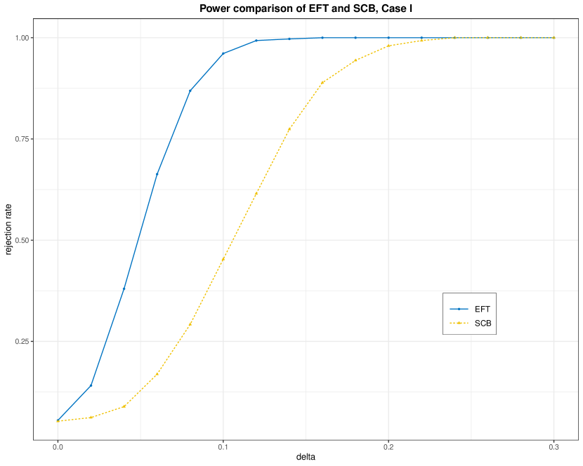
Figure 1: Power of EFT and SCB: Case I

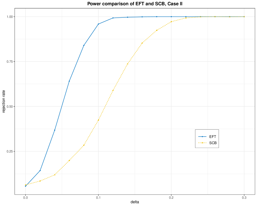
Figure 2: Power of EFT and SCB: Case II

5.3 Lack-of-fit Test

For an illustration of the Lack-of-fit Test, we focus on $\beta_{1}(t)$ in Case I and Case II. Under both settings, $\beta_{1}(t)=0.5$ satisfies constancy and linearity, thus the two types of Lack-of-fit Tests can be conducted to demonstrate the accuracy of our method. Following the procedures described in Section 4.2, we obtain the simulated type I errors for the 4 losses and sample size $N=300,500$. The optimal bandwidths are exactly the same as those selected in Section 5.2 in that we are considering the same settings. We can see from Table 3 and Table 4 that the accuracy of the Lack-of-fit Test is quite satisfactory and is not very sensitive to the selection of the bandwidths.

Table 3: Simulated type I error of constancy test of $\beta_{1}(t)$ in Case I and II.

$L_{2}$ $\tau=0.15$ $\tau=0.5$ $\tau=0.85$ Case I Case II Case I Case II Case I Case II Case I Case II $\alpha$ $5\%$ $10\%$ $5\%$ $10\%$ $5\%$ $10\%$ $5\%$ $10\%$ $5\%$ $10\%$ $5\%$ $10\%$ $5\%$ $10\%$ $5\%$ $10\%$ $N=300$ $b/1.15$ $5.1$ $8.6$ $5.0$ $10.0$ $5.4$ $8.9$ $5.6$ $10.0$ $5.0$ $8.7$ $5.0$ $8.8$ $5.1$ $8.9$ $5.6$ $10.7$ $b$ $5.0$ $9.1$ $6.1$ $10.2$ $6.0$ $9.1$ $5.7$ $10.2$ $5.3$ $9.4$ $5.6$ $9.5$ $5.4$ $9.0$ $5.6$ $9.9$ $1.15b$ $4.4$ $8.0$ $6.0$ $9.4$ $4.7$ $8.0$ $5.8$ $9.6$ $5.2$ $9.1$ $5.9$ $10.2$ $5.3$ $9.8$ $6.5$ $10.2$ $N=500$ $b/1.15$ $5.9$ $9.2$ $4.7$ $9.6$ $6.1$ $10.3$ $5.5$ $10.6$ $5.0$ $9.1$ $5.9$ $9.6$ $6.7$ $10.8$ $5.9$ $9.5$ $b$ $5.2$ $9.1$ $6.0$ $11.2$ $6.1$ $9.7$ $6.2$ $10.8$ $5.4$ $8.8$ $6.1$ $9.8$ $5.9$ $9.5$ $6.0$ $9.8$ $1.15b$ $5.6$ $9.9$ $5.1$ $10.0$ $5.4$ $9.0$ $5.9$ $10.6$ $5.5$ $9.1$ $5.1$ $9.6$ $6.6$ $10.3$ $6.1$ $9.6$

Table 4: Simulated type I error of linearity test of $\beta_{1}(t)$ in Case I and II.

$L_{2}$ $\tau=0.15$ $\tau=0.5$ $\tau=0.85$ Case I Case II Case I Case II Case I Case II Case I Case II $\alpha$ $5\%$ $10\%$ $5\%$ $10\%$ $5\%$ $10\%$ $5\%$ $10\%$ $5\%$ $10\%$ $5\%$ $10\%$ $5\%$ $10\%$ $5\%$ $10\%$ $N=300$ $b/1.15$ $4.6$ $8.5$ $5.6$ $9.5$ $5.4$ $9.8$ $5.5$ $9.5$ $5.7$ $10.8$ $5.9$ $9.7$ $6.0$ $9.1$ $6.0$ $10.5$ $b$ $4.5$ $8.3$ $6.5$ $9.8$ $6.3$ $8.9$ $5.0$ $9.1$ $5.6$ $9.4$ $5.7$ $9.7$ $6.1$ $10.2$ $5.4$ $9.7$ $1.15b$ $5.6$ $8.8$ $6.6$ $9.6$ $5.8$ $9.5$ $5.6$ $8.7$ $5.0$ $9.3$ $5.5$ $10.3$ $5.8$ $9.0$ $5.4$ $9.9$ $N=500$ $b/1.15$ $5.3$ $9.0$ $6.3$ $10.0$ $5.0$ $8.9$ $5.5$ $9.1$ $5.6$ $9.0$ $5.3$ $9.3$ $5.9$ $10.2$ $5.6$ $9.6$ $b$ $5.9$ $8.9$ $6.4$ $10.5$ $5.7$ $9.1$ $5.6$ $9.1$ $6.8$ $9.9$ $6.0$ $9.5$ $5.5$ $10.4$ $6.0$ $10.2$ $1.15b$ $5.2$ $9.0$ $5.3$ $9.9$ $6.2$ $10.3$ $6.0$ $9.9$ $5.7$ $9.0$ $6.8$ $10.6$ $5.8$ $10.6$ $5.1$ $8.9$

Under the setting of Case II, we also conducted the power analysis under 2 scenarios: (1) $\beta_{1}(t)=0.5+\delta t$; (2) $\beta_{1}(t)=0.5+\delta t^{2}$, where the first scenario allows us to investigate constancy while the other enables the testing of linearity. The sample size is chosen to be $N=500$ and the nominal level is $5\%$. For each test, power curves regarding the 4 different losses are simulated and compared in Figure 4 and Figure 4. The quadratic loss is the most powerful and the quantile loss with $\tau=0.5$ comes second. As for the extreme quantiles $\tau=0.15$ and $\tau=0.85$, the convergence is relatively slower.

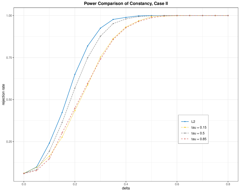
Figure 3: Power of LOFT: Constancy

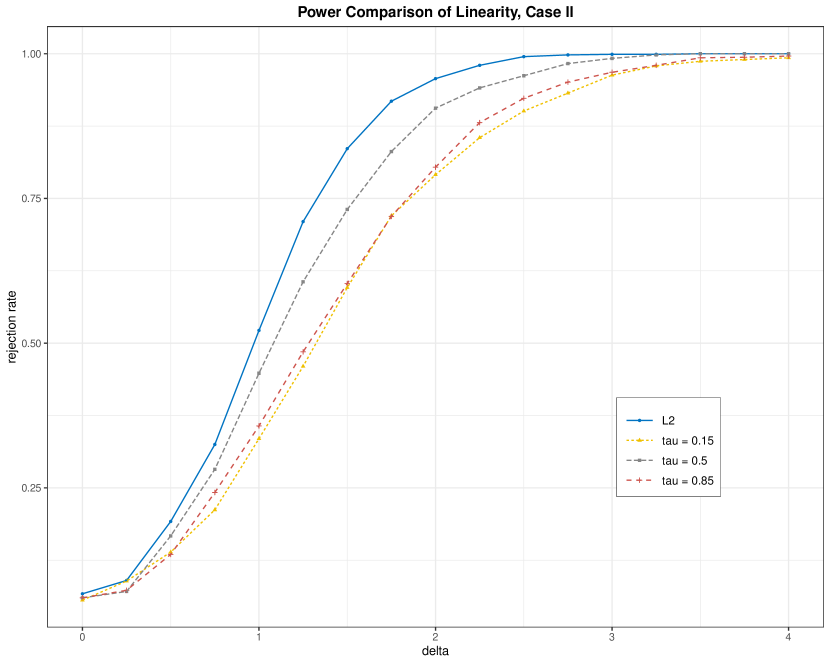
Figure 4: Power of LOFT: Linearity

We then compare our method with Chen and Hong, (2012) for the test of constancy of the coefficients. Since their method assumes stationary covariates and errors, we consider the following stationary model for a more fair comparison:

1. $y_{i}=\delta\cdot\sin(2\pi t_{i})+0.5x_{i,1}+\delta\cdot 2\log(1+2t_{i})x_{i,2}+e_{i}$, where $x_{i,1}=0.5x_{i-1,1}+\varepsilon_{i}$, $x_{i,2}=0.5x_{i-1,2}+\eta_{i}$, and $\{\varepsilon_{i}\},\{\eta_{i}\},\{e_{i}\}$ are i.i.d standard normal random variables independent of each other.

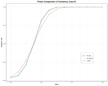
Figure 5: Power comparison of LOFT

Note that when $\delta=0$, the model corresponds to constant coefficients $\mbox{\boldmath$\beta$}(t)=(0,0.5,0)^{\top}$, and for the joint constancy test of $\mbox{\boldmath$\beta$}(t)$, we expect to see an increasing rejection rate as $\delta\geq 0$ increases. We generate the data under $N=500$ and use $L_{2}$ loss for the implementation of our method. The nominal level is chosen as $\alpha=5\%$. Figure 5 indicates that our method has comparable accuracy and power with Chen and Hong, (2012)’s method, where ‘H-homo’ and ‘H-het’ represent the homoscedastic and heteroscedasticity-robust version of the generalized Hausman test proposed in Chen and Hong, (2012). Considering that their method is designed for the constancy test of $L_{2}$-regression models and applies to stationary variables, our Lack-of-fit Test enjoys more flexibility and broader applicability, with a faster convergence rate theoretically.

5.4 Qualitative Test

For the Qualitative Test, exemplarily, we mainly focus on the hypothesis of monotonicity. Under the setting of Case II with $N=500$, we generate the data using the following mechanism: $\beta_{1}(t)=0.5-\delta\cdot 10\exp(-(t-0.5)^{2})$ for $\delta\geq 0$, and we expect to see an increasing power curve as $\delta$ increases.

Applying a similar projection idea to the SCB test in Wu and Zhou, (2017), we also manage to obtain the power curve regarding the monotonicity test for quantile loss with $\tau=0.5$ for their method. Figure 7 Provides the results with nominal level $\alpha=5\%$, demonstrating the performance of our method regarding 4 losses and the comparison with the SCB test. The power curves of quadratic loss and quantile loss with $\tau=0.5$ converge faster than the extreme quantiles, as we expect. Figure 7 also shows that, under the same quantile loss with $\tau=0.5$, our qualitative test is more powerful than the SCB test with projection. This is due to the fact that our CRF-based test can detect local alternatives of the order $O(1/\sqrt{n})$ where the SCB in Wu and Zhou, (2017) are sensitive to those of the order $O(\sqrt{\log n}/\sqrt{nb_{n}})$ with bandwidth $b_{n}\rightarrow 0$.

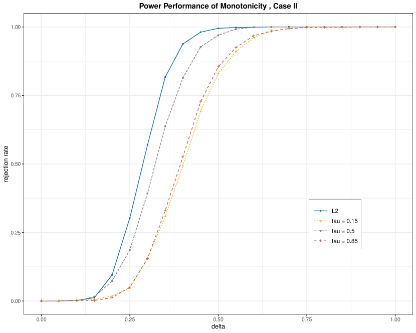
Figure 6: Power of QT under different losses

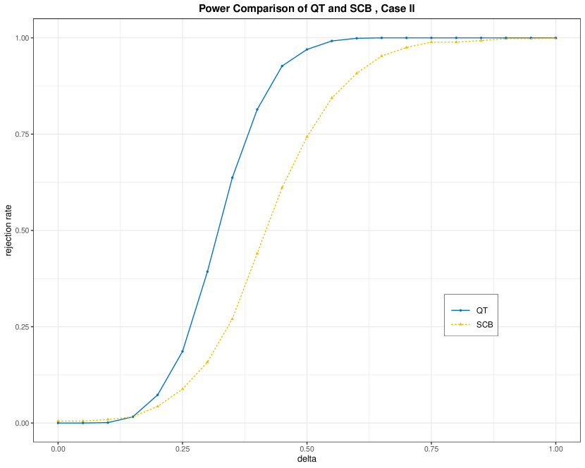
Figure 7: Power of QT and SCB

6 A Real Data Illustration

In this section, we delve into monthly global temperature anomalies from 1882.1 to 2005.12 (available at HadCRUT5 dataset), investigating the anthropogenic warming trend and the time-varying relationship between the anomalies and potential factors. The initial candidate factors include lags of multivariate ENSO index (MEI), total solar irradiance (TSI), aerosol optical depth (AOD) and Atlantic multidecadal oscillation (AMO). These factors are typical regressors in existing studies, where multivariate linear regression is commonly employed to filter out the fluctuations caused by the factors and to reveal the underlying anthropogenic warming (Zhou and Tung,, 2013). The authors believe that the warming trend has been remarkably steady since the mid-twentieth century. Foster and Rahmstorf, (2011) also applied a similar approach to the global temperature anomalies from 1979 to 2010, where the deduced warming rate was also found to be steady over the investigated time interval. All previous analyses assume a stationary structure of the errors and constant coefficients over time, in addition to which a linear trend of anthropogenic warming is also hypothesized. Nevertheless, by utilizing the change-point detection method in (Zhou,, 2013), nonstationarity of the residuals has been detected after fitting the multivariate linear model, suggesting the necessity to use a more general model that allows for the nonstationarity of the time series. Furthermore, no rigorous proof has been provided in the existing literature to draw convincing conclusions about the shape of the warming trend.

We hereby apply our method to the aforementioned time series. Following the steps described in Section 4, a full model consisting of all the factors is first constructed and analyzed, then a backward variable selection procedure is implemented based on our EFT. Most covariates are therefore removed due to insignificance or multicollinearity. The final model includes the intercept, MEI, and the 6-month lag of MEI under $L_{2}$ loss, quantile loss with $\tau=0.15$ and $\tau=0.5$, while the $\tau=0.85$ quantile regression model is composed of the intercept, 2-month and 6-month lags of MEI, and 5-month lag of AOD. All models involve the intercept and corresponding lags of MEI, enabling us to later conduct tests regarding the anthropogenic warming trend and the coefficient of the ENSO effect. The outcome agrees with the fact that ENSO has conventionally been recognized as a leading contributor to global temperature fluctuations (Trenberth et al.,, 2002; Foster and Rahmstorf,, 2011). The 6-month lag of MEI chosen in each model also aligns with the belief that El Niño warms up the global temperature with a lag of $\sim$6 months (Trenberth et al.,, 2002). As a distinctive predictor, the 5-month lag of AOD is selected under the $\tau=0.85$ quantile loss, which emphasizes the influence of volcano activities on extreme high temperatures. The model selection result also coincides with vast literature in climatology, where ENSO and volcano events are identified as significant sources of variance in global temperature, compared to solar activities and other factors (Lean and Rind,, 2008; Foster and Rahmstorf,, 2011). On the other hand, however, our conclusion is drawn under general non-stationary assumptions which could be more reliable.

Table 5: Tests of monotonicity (increasing), linearity and constancy.

$\text{Intercept},\text{Monotonicity}$ $\text{Intercept},\text{Linearity}$ $\text{MEI or MEI (lag 2)},\text{Constancy}$ $\text{MEI (lag 6)},\text{Constancy}$ Test Statistic ${95\%}\text{ C.V.}$ p-value Test Statistic ${95\%}\text{ C.V.}$ p-value Test Statistic ${95\%}\text{ C.V.}$ p-value Test Statistic ${95\%}\text{ C.V.}$ p-value $L_{2}$ 0.132 1.355 1 0.853 0.69 0.007 0.217 0.702 0.986 0.221 0.499 0.842 $\tau=0.15$ 0.157 1.02 1 0.886 0.647 0.002 0.401 0.711 0.613 0.4 0.528 0.244 $\tau=0.5$ 0.143 1.464 1 0.877 0.752 0.013 0.333 0.729 0.804 0.216 0.643 0.978 $\tau=0.85$ 0.293 1.495 0.999 0.954 0.733 0.001 0.322 0.527 0.468 0.431 0.496 0.121

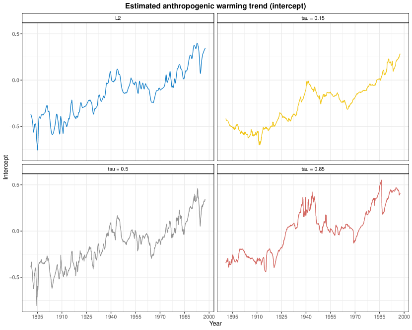
Figure 8: Estimated warming trend

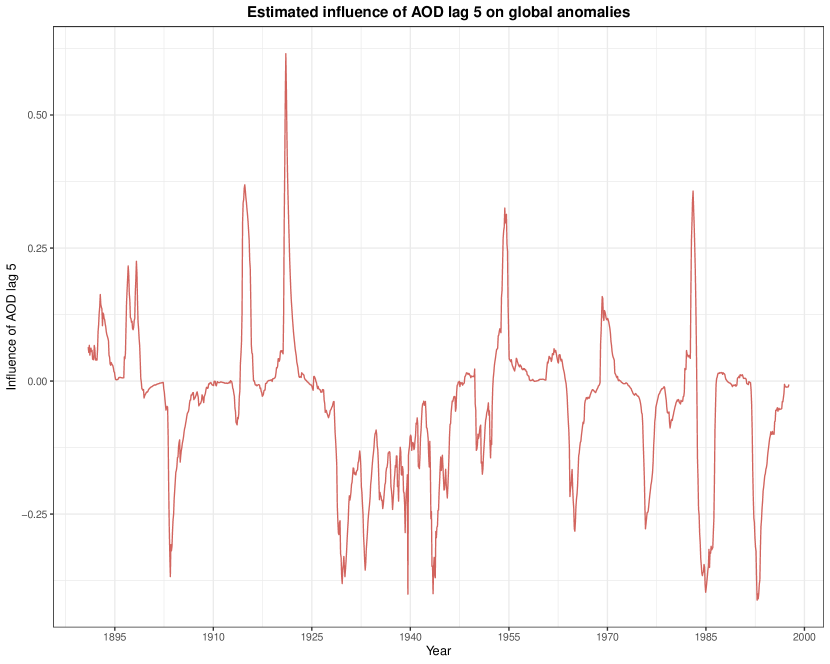
Figure 9: Influence of the 5-month lag of AOD

The hypotheses that we are interested in are the shape of the anthropogenic trend and the coefficients regarding MEI and AOD. It is commonly believed that the anthropogenic trend is increasing, and we can further check whether it is steady over time, which is equivalent to testing whether the intercept is a linear function. As for the coefficients related to MEI and AOD, we examine whether they are time-invariant, which amounts to testing the constancy. The test results are summarized in Table 5, which demonstrates the similarity of the results under different losses. For the shape of the intercept, the positive monotonicity is not rejected, while the linearity is rejected at $5\%$ significance level. This strengthens the belief of discernible human influences on global warming and also suggests that the warming rate is not steady from 1882 to 2005. The non-uniform rate is consistent with the conclusion from IPCC, (2007), where global warming is observed to accelerate until 2005 after a cooling period in the 1960s and 1970s. This can also be illustrated by Figure 9, with a relatively flat trend from 1960 to 1970, and a steep increase afterward. While a similar pattern can be detected by solely analyzing the temperature anomalies, our approach rigorously assesses the anthropogenic fluctuations by separating them from the natural ones, thus making the conclusion more reliable and statistically verifiable. As for the coefficients of MEI and its lags, we fail to reject the null hypothesis of constancy at $5\%$ significance level. This gives us the insight that the overall ENSO effect on global temperature is likely to be steady from 1882 to 2005.

To represent the temperature change induced by volcano activities, we demonstrate the influence of the 5-month lag of AOD in Figure 9, which is computed by multiplying the estimated coefficient and the factor itself. Unlike the traditional multivariate linear regression where only the overall negative effect of AOD can be statistically detected, Figure 9 reveals the effect of AOD as a combination of heating and long-term cooling. This finding complies with the mechanism of volcano activities, where volcano eruptions can cool the surface due to an increased aerosol loading in the stratosphere that scatters solar radiation back to space. Simultaneously, these eruptions can lead to regional heating, particularly evident during winters in the Northern Hemisphere (Robock,, 2000; Christiansen,, 2008). Such unstable and complicated impact is also confirmed using our Lack-of-fit Test, where the $p$-values obtained for the test of constancy and linearity turn out to be 0.029 and 0.002, respectively.

7 Assumptions and Auxiliary Theoretical Results

Let $z_{i}(t)=y_{i}-{\bf x}_{i}^{\top}\mbox{\boldmath$\beta$}(t)-{\bf x}_{i}^{\top}\mbox{\boldmath$\beta$}^{\prime}(t)(t_{i}-t)$, and define

$$\tilde{\mbox{\boldmath$\theta$}}_{b_{n}}(t):=\left(\begin{array}[]{c}\hat{\mbox{\boldmath$\theta$}}_{b_{n}}(t)\\ \hat{\mbox{\boldmath$\theta$}}_{b_{n}}^{\prime}(t)\end{array}\right)=\mathop{\mbox{argmin}}_{\mbox{\boldmath$c$}_{0},\mbox{\boldmath$c$}_{1}\in\mathbb{R}^{p}}\sum_{i=1}^{n}\rho(z_{i}(t)-{\bf x}_{i}^{\top}\mbox{\boldmath$c$}_{0}-{\bf x}_{i}^{\top}\mbox{\boldmath$c$}_{1}(t_{i}-t)/b_{n})K_{b_{n}}(t_{i}-t),$$ (26)

where $K_{b_{n}}(\cdot):=K(\cdot/b_{n})$. Compare this with equation (7), simple calculations yield that

$$\hat{\mbox{\boldmath$\theta$}}_{b_{n}}(t)=\hat{\mbox{\boldmath$\beta$}}_{b_{n}}(t)-\mbox{\boldmath$\beta$}(t),\quad\hat{\mbox{\boldmath$\theta$}}_{b_{n}}^{\prime}(t)=b_{n}(\hat{\mbox{\boldmath$\beta$}}_{b_{n}}^{\prime}(t)-{\mbox{\boldmath$\beta$}}^{\prime}(t)).$$ (27)

Let $\mbox{\boldmath$\theta$}=(\mbox{\boldmath$\theta$}_{0}^{\top},\mbox{\boldmath$\theta$}_{1}^{\top})^{\top}=(\theta_{01},\theta_{02},\cdots\theta_{0p},\theta_{11},\theta_{12},\cdots,\theta_{1p})^{\top}$ be a $(2p\times 1)$ vector, $\mathbf{w}_{in}(t)=\left(\mathbf{x}_{i}^{\top},\mathbf{x}_{i}^{\top}(i/n-t)/b_{n}\right)^{\top}\allowbreak=\left(w_{in,1}(t),\ldots,w_{in,2p}(t)\right)^{\top}$. Write $\eta_{i}(t,\mbox{\boldmath$\theta$})=\psi(z_{i}(t)-\mathbf{w}_{in}^{\top}(t)\mbox{\boldmath$\theta$})K_{b_{n}}(t_{i}-t)$, $S_{n}(t,\mbox{\boldmath$\theta$})=\sum_{i=1}^{n}\eta_{i}(t,\mbox{\boldmath$\theta$})\mathbf{w}_{in}(t)$. We assume $\sup_{t\in(0,1)}S_{n}(t,\tilde{\mbox{\boldmath$\theta$}}_{b_{n}}(t))=O_{\mathbb{P}}(\log n)$.

Remark 2.

The assumption $\sup_{t\in(0,1)}S_{n}(t,\tilde{\mbox{\boldmath$\theta$}}_{b_{n}}(t))=O_{\mathbb{P}}(\log n)$ controls the magnitude of $S_{n}(t,\tilde{\mbox{\boldmath$\theta$}}_{b_{n}}(t)$, which is used to establish the Bahadur representation. If $\psi(\cdot)$ is continuous, this assumption is automatically satisfied as $\sup_{t\in(0,1)}S_{n}(t,\tilde{\mbox{\boldmath$\theta$}}_{b_{n}}(t))=0$. While in the case where $\psi(\cdot)$ is discontinuous, the solution may not always exist. A key example of such discontinuous $\psi(\cdot)$ arises in quantile regression (Wu,, 2007, Remark 4) and the proof of it for quantile regression is provided in Lemma LABEL:lem:4 of the supplementary.

7.1 Model Assumptions

For $q\geq 0,j=0,1,\cdots,r$, define for $t\in(w_{j},w_{j+1}]$,

$$\Xi_{j}^{(q)}\left(t,x\mid\mathcal{F}_{k-1},\mathcal{G}_{k}\right) = \dfrac{\partial^{q}}{\partial x^{q}}\mathbb{E}\left\{\psi\left(G_{j}\left(t,\mathcal{F}_{k},\mathcal{G}_{k}\right)+x\right)\mid\mathcal{F}_{k-1},\mathcal{G}_{k}\right\},$$

$$\bar{\kappa}_{j}\left(t,x\mid\mathcal{G}_{k}\right) = \dfrac{\partial}{\partial x}\mathbb{E}\left(\psi\left(G_{j}\left(t,\mathcal{F}_{k},\mathcal{G}_{k}\right)+x\right)\mid\mathcal{G}_{k}\right).$$

• For $0\leq j\leq r$, assume that

  $$\sup_{t\in(w_{j},w_{j+1}),x,y,\in\mathbb{R}}|\Xi_{j}(t,x\mid\mathcal{F}_{-1},\mathcal{G}_{0})-\Xi_{j}(t,y\mid\mathcal{F}_{-1},\mathcal{G}_{0})|$$ (28)

  $$\leq C_{j,1}|x-y|+C_{j,2}|x^{2}-y^{2}|+C_{j,3}|x-y|^{2},$$ (29)

  where $C_{j,1},C_{j,2},C_{j,3}$ are $(\mathcal{F}_{-1},\mathcal{G}_{0})$ measurable r.v. with finite fourth moments. We also require that for $0\leq j\leq r$, $\Xi_{j}^{(1)}(t,0\mid\mathcal{F}_{-1},\mathcal{G}_{0})$ is stochastically Lipschitz continuous for $t\in(w_{j},w_{j+1}]$, that is, $\exists M<\infty$, s.t. $\forall t_{1},t_{2}\in(w_{j},w_{j+1}]$, $0\leq j\leq r$,

  $$||\Xi_{j}^{(1)}(t_{1},0\mid\mathcal{F}_{-1},\mathcal{G}_{0})-\Xi_{j}^{(1)}(t_{2},0\mid\mathcal{F}_{-1},\mathcal{G}_{0})||\leq M|t_{1}-t_{2}|.$$ (30)

• Assume for the covariate process, $\exists t_{x}>0$, s.t. $\max_{1\leq i\leq n}\mathbb{E}(\exp(t_{x}|\mathbf{x}_{i}|))\leq\infty$. In addition, $\max_{1\leq j\leq r}\sup_{t\in(w_{j},w_{j+1}]}||{\bf H}_{j}(t,\mathcal{G}_{i})-{\bf H}_{j}(t,\mathcal{G}_{i}^{*})||_{1}=O(\chi^{|i|})$ for some constant $\chi\in(0,1)$. For all $t_{1},t_{2}\in(w_{j},w_{j+1}],0\leq j\leq r$, $||{\bf H}_{j}(t_{1},\mathcal{G}_{0})-{\bf H}_{j}(t_{2},\mathcal{G}_{0})||\leq M|t_{1}-t_{2}|$ for some constant $M<\infty$. Recall the definition of $\mathcal{G}_{i}^{*}$ in Section 2.1.

• For $\epsilon\in\mathbb{R}$, $0\leq q\leq 2p+1$ and any integer $s$, define

  $$\delta_{s}^{(q)}(k-1,\epsilon):=\max_{0\leq j\leq r}\sup_{t\in(w_{j},w_{j+1}],|x|\leq\epsilon}||\Xi_{j}^{(q)}\left(t,x\mid\mathcal{F}_{k-1},\mathcal{G}_{k}\right)-\Xi_{j}^{(q)}\left(t,x\mid\mathcal{F}_{k-1}^{*},\mathcal{G}_{k}\right)||_{s}.$$

  We assume that $\exists\epsilon_{0}\in\mathbb{R}$, s.t. $\delta_{1}^{(q)}(k-1,\epsilon_{0})=O(\chi^{|k-1|})$ for some constant $0<\chi<1$.

• Define $\bar{\Xi}^{(q)}(x\mid\mathcal{G}_{i})=\frac{\partial^{q}}{\partial x^{q}}\mathbb{E}[\psi(e_{i}+x)\mid\mathcal{G}_{i}]$, we require for all $i=1,2,\cdots,n$ and any $p$-dimensional vector $\mathbf{h}$ that

  $$\bar{\Xi}(0\mid\mathcal{G}_{i})=\mathbb{E}[\psi(e_{i})\mid\mathcal{G}_{i}]=0,a.s.$$

  $$\bar{\Xi}(\mathbf{x}^{\top}_{i}\mathbf{h}\mid\mathcal{G}_{i})=\bar{\Xi}^{(1)}(0\mid\mathcal{G}_{i})\mathbf{x}^{\top}_{i}\mathbf{h}+O_{\mathbb{P}}(|\mathbf{x}_{i}^{2}||\mathbf{h}|^{2}),$$

  and $\bar{\Xi}^{(1)}(x\mid\mathcal{G}_{i})>0$ a.s. for $|x|\leq\epsilon$ for some $\epsilon>0$. Let $\bar{\lambda}_{n}(t)$ be the smallest eigenvalue of $\mathbb{E}\{\sum_{i=1}^{n}\bar{\Xi}^{(1)}(0\mid\mathcal{G}_{i})\}\mathbf{x}_{i}\mathbf{x}^{\top}_{i}K_{b_{n}}(t_{i}-t)\}$, assume that $\liminf_{n\to\infty}\inf_{t\in(0,1)}\frac{\bar{\lambda}_{n}(t)}{nb_{n}}>0$. Let $\lambda(t)$ be the smallest eigenvalue of $\Sigma(t):=\mathbb{E}\{\bar{\kappa}_{j}\left(t,0\mid\mathcal{G}_{i}\right){\bf H}_{j}(t,\mathcal{G}_{i}){\bf H}_{j}^{\top}(t,\mathcal{G}_{i})\}$ if $t\in(w_{j},w_{j+1}]$. We require that i) $\max_{0\leq j\leq r}\sup_{t\in(w_{j},w_{j+1}]}||\bar{\kappa}_{j}\left(t,0\mid\mathcal{G}_{i}\right)-\bar{\kappa}_{j}\left(t,0\mid\mathcal{G}_{i}^{*}\right)||=O(\chi^{|i|})$ for some constant $\chi\in(0,1)$, and $\max_{0\leq j\leq r}\sup_{t\in(w_{j},w_{j+1}]}|{\bar{\kappa}}_{j}\left(t,0\mid\mathcal{G}_{0}\right)|\leq M$ a.s. for some constant $M<\infty$; ii) $\inf_{t\in(0,1)}\lambda(t)\geq\eta>0$ for some positive constant $\eta$; iii) $\max_{0\leq j\leq r}\sup_{t\in(w_{j},w_{j+1}]}||\dot{\bar{\kappa}}_{j}\left(t,0\mid\mathcal{G}_{i}\right)-\dot{\bar{\kappa}}_{j}\left(t,0\mid\mathcal{G}_{i}^{*}\right)||=O(\chi^{|i|})$ for some constant $\chi\in(0,1)$, and $\max_{0\leq j\leq r}\sup_{t\in(w_{j},w_{j+1}]}|\dot{\bar{\kappa}}_{j}\left(t,0\mid\mathcal{G}_{0}\right)|\leq M$ a.s. for some constant $M<\infty$, where $\dot{\bar{\kappa}}_{j}\left(t,0\mid\mathcal{G}_{i}\right):=\frac{\partial}{\partial t}\bar{\kappa}_{j}\left(t,0\mid\mathcal{G}_{i}\right)$.

• Assume $\delta_{{\bf W}}(k,4)=O(\chi^{k})$ for some $\chi\in(0,1)$, where $\mathbf{W}(t,\mathcal{F}_{i},\mathcal{G}_{i})={\bf H}_{j}(t,\mathcal{G}_{i})\psi(G_{j}(t,\mathcal{F}_{i},\mathcal{G}_{i}))$ if $t\in(w_{j},w_{j+1}]$, $j=0,\cdots,r$. Also assume for the error process that $\sup_{i}||\psi(G_{j}(t,\mathcal{F}_{i},\mathcal{G}_{i}))||_{4}<\infty$ for all $j=0,\cdots,r$ and $t\in(w_{j},w_{j+1}]$. Further assume for all $t_{1},t_{2}\in(w_{j},w_{j+1}],0\leq j\leq r$, $||\psi(G_{j}(t_{1},\mathcal{F}_{0},\mathcal{G}_{0}))-\psi(G_{j}(t_{2},\mathcal{F}_{0},\mathcal{G}_{0}))||\leq M|t_{1}-t_{2}|$ for some constant $M<\infty$.

• Define the long-run covariance function of $\{\mathbf{W}_{i}:=\mathbf{W}(t_{i},\mathcal{F}_{i},\mathcal{G}_{i})=\mathbf{x}_{i}\psi(e_{i})\}$

  $$\Psi(t)=\sum_{i=-\infty}^{\infty}\mbox{ Cov}[\mathbf{W}(t,\mathcal{F}_{0},\mathcal{G}_{0}),\mathbf{W}(t,\mathcal{F}_{i},\mathcal{G}_{i})].$$

  Let $\Psi(0)=\lim_{t\downarrow 0}\Psi(t)$. Assume that the minimum eigenvalue of $\Psi(t)$ is bounded away from 0 on $[0,1]$.

• Define $\Sigma_{m}=\sum_{i=1}^{m}\Sigma^{-1}(t_{i})\Psi(t_{i})\Sigma^{-1}(t_{i})$. Assume that, for sufficiently large $n$, there exists $L<\infty$, such that $|\Sigma_{\lfloor s_{1}n\rfloor}-\Sigma_{\lfloor s_{2}n\rfloor}|\leq L(\lfloor s_{2}n\rfloor-\lfloor s_{1}n\rfloor)$ holds for $0<s_{1}<s_{2}<1$.

Here are some insights on the above regularity conditions. Assumption (A1) guarantees the smoothness of the conditional loss functions. (28) holds if $\sup_{t\in(0,1)}|\psi^{(1)}(t)|<\infty$, which is satisfied by least square regression, and can be achieved by quantile regression under some mild constraints. A sufficient condition for (28) is provided in Wu and Zhou, (2018) by virtue of the robustness of loss functions. (A2) requires that the covariate process is stochastic Lipschitz continuous with geometrically decaying dependence measures. The moment requirement of $\mathbf{x}_{i}$ in (A2) can also be significantly relaxed when $\psi(\cdot)$ is bounded or light-tailed. (A3) controls the dependence measures of the derivatives of the loss functions’ conditional expectations, and is easy to verify for a large class of non-stationary processes, see Wu and Zhou, (2018) for further details. (A4) plays an important role in the consistency of $\check{\mbox{\boldmath$\beta$}}(t)$ by endowing smoothness on $\bar{\Xi}(\cdot\mid\mathcal{G}_{i})$ to some extent. These conditions altogether enable Bahadur representation of the estimators. Condition (A6) means that the time-varying long-run covariance matrices of $\{\mathbf{W}_{i}\}_{i=1}^{n}$ are non-degenerate on $[0,1]$, see also Wu and Zhou, (2017). (A7) assumes Lipschitz continuity of $\Sigma_{m}$. This assumption is utilized to guarantee the tightness of the estimators, see Lemma LABEL:lem:7 in the supplementary material for more details.

7.2 Uniform Bahadur Representation

This section establishes uniform Bahadur representations for the local linear M-estimators and the estimated CRF, by which the limiting distribution of the estimators can be derived in conjunction with some Gaussian approximation results.

Define a $2p\times 2p$ matrix $\Sigma_{1}(t)=\leavevmode\resizebox{72.0pt}{}{$\begin{pmatrix}\Sigma(t)&0\\ 0&\mu_{2}\Sigma(t)\end{pmatrix}$}$, where $\Sigma(t)$ is defined in (A4) and $\mu_{k}:=\int|x|^{k}K(x)\,dx$ for some positive integer $k$.

Theorem 4.

Suppose (A1)-(A4), $\frac{nb_{n}^{4}}{\log^{8}n}\to\infty$, and $n^{c}b_{n}\to 0$ for some positive constant $c$. Let $\mathfrak{T}_{n}=\left[b_{n},1-b_{n}\right]$, and $\mathfrak{T}_{n}^{\prime}=\mathfrak{T}_{n}\setminus\cup_{j=1}^{r}[w_{j}-b_{n},w_{j}+b_{n}]$, then

$$\sup_{t\in\mathfrak{T}_{n}^{\prime}}\left|\Sigma_{1}(t)\tilde{\mbox{\boldmath$\theta$}}_{b_{n}}(t)-\frac{\sum_{i=1}^{n}\psi\left(z_{i}(t)\right)\mathbf{w}_{in}(t)K_{b_{n}}(i/n-t)}{nb_{n}}\right|=O_{\mathbb{P}}\left(\frac{\pi_{n}}{\sqrt{nb_{n}}}\right),$$ (31)

where $\pi_{n}=b_{n}\log^{6}n+(nb_{n})^{-\frac{1}{4}}\log^{3}n+\sqrt{nb_{n}}b_{n}^{3}\log^{3}n$.

The Bahadur representation in (31) involves a bias term involving $\mbox{\boldmath$\beta$}^{\prime\prime}(t)$. Recall the Jackknife bias-corrected M-estimator $\check{\Lambda}(t)$ defined in (8) and (9). We extend the above Bahadur representation result to the estimated CRF as follows.

Corollary 1.

Suppose the conditions of Theorem 4 hold, then for any $s\times p$, $s\leq p$ full rank matrix $\mathbf{C}$, $\pi_{n}=b_{n}\log^{6}n+(nb_{n})^{-\frac{1}{4}}\log^{3}n+\sqrt{nb_{n}}b_{n}^{3}\log^{3}n$,

$$\sup_{t\in\mathfrak{T}_{n}}\left|\sqrt{n}\mathbf{C}\left(\check{\Lambda}(t)-{\Lambda}(t)\right)-\frac{1}{\sqrt{n}}\sum_{i=1}^{\lfloor nt\rfloor}\mathbf{C}\Sigma^{-1}\left(t_{i}\right)\psi\left(e_{i}\right)\mathbf{x}_{i}\right|=O_{\mathbb{P}}\left(\frac{\pi_{n}}{\sqrt{b_{n}}}\right).$$

References

• Akakpo et al., (2014) Akakpo, N., Balabdaoui, F., and Durot, C. (2014). Testing monotonicity via local least concave majorants. Bernoulli, 20(2):514 – 544.
• Bickel and Ritov, (1988) Bickel, P. J. and Ritov, Y. (1988). Estimating integrated squared density derivatives: sharp best order of convergence estimates. Sankhya A (1961-2002), 50(3):381–393.
• Bowman et al., (1998) Bowman, A. W., Jones, M. C., and Gijbels, I. (1998). Testing monotonicity of regression. J. Comput. Graph. Stat., 7(4):489–500.
• Chen and Hong, (2012) Chen, B. and Hong, Y. (2012). Testing for smooth structural changes in time series models via nonparametric regression. Econometrica, 80(3):1157–1183.
• Christiansen, (2008) Christiansen, B. (2008). Volcanic eruptions, large-scale modes in the northern hemisphere, and the el niño–southern oscillation. Journal of Climate, 21(5):910–922.
• Dahlhaus, (2012) Dahlhaus, R. (2012). Locally stationary processes. volume 30 of Handbook of Statistics, pages 351–413. Elsevier.
• Dahlhaus et al., (2019) Dahlhaus, R., Richter, S., and Wu, W. B. (2019). Towards a general theory for nonlinear locally stationary processes. Bernoulli, 25(2):1013 – 1044.
• Dette et al., (2011) Dette, H., Preuß, P., and Vetter, M. (2011). A measure of stationarity in locally stationary processes with applications to testing. J. Am. Statist. Ass., 106(495):1113–1124.
• Diciccio and Romano, (1988) Diciccio, T. J. and Romano, J. P. (1988). A review of bootstrap confidence intervals. J. R. Statist. Soc. B, 50(3):338–354.
• Durot, (2003) Durot, C. (2003). A Kolmogorov-type test for monotonicity of regression. Statist. Probab. Lett., 63(4):425–433.
• Ebi et al., (2021) Ebi, K. L., Vanos, J., Baldwin, J. W., Bell, J. E., Hondula, D. M., Errett, N. A., Hayes, K., Reid, C. E., Saha, S., Spector, J., and Berry, P. (2021). Extreme weather and climate change: population health and health system implications. Annu. Rev. Public Health, 42(1):293–315.
• Fan and Zhang, (1999) Fan, J. and Zhang, W. (1999). Statistical estimation in varying coefficient models. Ann. Statist., 27(5):1491 – 1518.
• Fan and Zhang, (2000) Fan, J. and Zhang, W. (2000). Simultaneous confidence bands and hypothesis testing in varying-coefficient models. Scandinavian Journal of Statistics, 27(4):715–731.
• Fang and Seo, (2021) Fang, Z. and Seo, J. (2021). A projection framework for testing shape restrictions that form convex cones. Econometrica, 89(5):2439–2458.
• Foster and Rahmstorf, (2011) Foster, G. and Rahmstorf, S. (2011). Global temperature evolution 1979–2010. Environ. Res. Lett., 6(4):044022.
• Francq and Sucarrat, (2023) Francq, C. and Sucarrat, G. (2023). Volatility estimation when the zero-process is nonstationary. J. Bus. Econ. Statist., 41(1):53–66.
• Friedman and Tibshirani, (1984) Friedman, J. and Tibshirani, R. (1984). The monotone smoothing of scatterplots. Technometrics, 26(3):243–250.
• Ghosal et al., (2000) Ghosal, S., Sen, A., and van der Vaart, A. W. (2000). Testing monotonicity of regression. Ann. Statist., 28(4):1054–1082.
• Gijbels et al., (2000) Gijbels, I., Hall, P., Jones, M. C., and Koch, I. (2000). Tests for monotonicity of a regression mean with guaranteed level. Biometrika, 87(3):663–673.
• Hall and Heckman, (2000) Hall, P. and Heckman, N. E. (2000). Testing for monotonicity of a regression mean by calibrating for linear functions. Ann. Statist., 28(1):20–39.
• Hall and Marron, (1987) Hall, P. and Marron, J. (1987). Estimation of integrated squared density derivatives. Statist. Probab. Lett., 6(2):109–115.
• Hardle and Mammen, (1993) Hardle, W. and Mammen, E. (1993). Comparing nonparametric versus parametric regression fits. Ann. Statist., 21(4):1926 – 1947.
• Hardle and Marron, (1991) Hardle, W. and Marron, J. S. (1991). Bootstrap simultaneous error bars for nonparametric regression. Ann. Statist., 19(2):778–796.
• Hastie and Tibshirani, (1993) Hastie, T. and Tibshirani, R. (1993). Varying-coefficient models. J. R. Statist. Soc. B, 55(4):757–796.
• He and Zhu, (2003) He, X. and Zhu, L.-X. (2003). A lack-of-fit test for quantile regression. J. Am. Statist. Ass., 98(464):1013–1022.
• Hong and White, (1995) Hong, Y. and White, H. (1995). Consistent specification testing via nonparametric series regression. Econometrica, 63(5):1133–1159.
• Hoover et al., (1998) Hoover, D. R., Rice, J. A., Wu, C. O., and Yang, L.-P. (1998). Nonparametric smoothing estimates of time-varying coefficient models with longitudinal data. Biometrika, 85(4):809–822.
• Huang and Fan, (1999) Huang, L.-S. and Fan, J. (1999). Nonparametric estimation of quadratic regression functionals. Bernoulli, 5(5):927 – 949.
• Huber, (1964) Huber, P. J. (1964). Robust estimation of a location parameter. Ann. Math. Stat., 35(1):73 – 101.
• Huber, (1973) Huber, P. J. (1973). Robust regression: asymptotics, conjectures and Monte Carlo. Ann. Statist., 1(5):799 – 821.
• I. Gijbels and Verhasselt, (2017) I. Gijbels, M. A. I. and Verhasselt, A. (2017). Shape testing in quantile varying coefficient models with heteroscedastic error. J. Nonparametr. Stat., 29(2):391–406.
• IPCC, (2007) IPCC (2007). Climate Change 2007: The Physical Science Basis. Contribution of Working Group I to the Fourth Assessment Report of the Intergovernmental Panel on Climate Change [Solomon, S., D. Qin, M. Manning, Z. Chen, M. Marquis, K.B. Averyt, M. Tignor and H.L. Miller (eds.)]. Cambridge university press, Cambridge.
• Knight, (2017) Knight, K. (2017). On the asymptotic distribution of the ${L}_{\infty}$ estimator in linear regression.
• Koenker, (2005) Koenker, R. (2005). Quantile Regression. Econometric Society Monographs. Cambridge University Press.
• Komarova and Hidalgo, (2020) Komarova, T. and Hidalgo, J. (2020). Testing nonparametric shape restrictions. (arXiv:1909.01675). arXiv:1909.01675 [econ, math, stat].
• Koul and Stute, (1999) Koul, H. L. and Stute, W. (1999). Nonparametric model checks for time series. Ann. Statist., 27(1):204 – 236.
• Kreiss and Paparoditis, (2014) Kreiss, J.-P. and Paparoditis, E. (2014). Bootstrapping Locally Stationary Processes. J. R. Statist. Soc. B, 77(1):267–290.
• Lean and Rind, (2008) Lean, J. L. and Rind, D. H. (2008). How natural and anthropogenic influences alter global and regional surface temperatures: 1889 to 2006. Geophys. Res. Lett., 35(18).
• Mies, (2023) Mies, F. (2023). Functional estimation and change detection for nonstationary time series. J. Am. Statist. Ass., 118(542):1011–1022.
• Nason, (2013) Nason, G. (2013). A Test for Second-Order Stationarity and Approximate Confidence Intervals for Localized Autocovariances for Locally Stationary Time Series. J. R. Statist. Soc. B, 75(5):879–904.
• Politis et al., (1999) Politis, D. N., Romano, J. P., and Wolf, M. (1999). Choice of the Block Size, pages 188–212. Springer New York, New York, NY.
• Robock, (2000) Robock, A. (2000). Volcanic eruptions and climate. Reviews of Geophysics, 38(2):191–219.
• Silverman, (1981) Silverman, B. W. (1981). Using kernel density estimates to investigate multimodality. J. R. Statist. Soc. B, 43(1):97–99.
• Stute, (1997) Stute, W. (1997). Nonparametric model checks for regression. Ann. Statist., 25(2):613 – 641.
• (45) Stute, W., Manteiga, W. G., and Quindimil, M. P. (1998a). Bootstrap approximations in model checks for regression. J. Am. Statist. Ass., 93(441):141–149.
• (46) Stute, W., Thies, S., and Zhu, L.-X. (1998b). Model checks for regression: an innovation process approach. Ann. Statist., 26(5):1916 – 1934.
• Trenberth et al., (2002) Trenberth, K. E., Caron, J. M., Stepaniak, D. P., and Worley, S. (2002). Evolution of El Niño–Southern Oscillation and global atmospheric surface temperatures. Journal of Geophysical Research: Atmospheres, 107(D8):AAC 5–1–AAC 5–17.
• Vogt, (2012) Vogt, M. (2012). Nonparametric regression for locally stationary time series. Ann. Statist., 40(5):2601–2633.
• Wu and Zhou, (2023) Wu, H.-T. and Zhou, Z. (2023). Frequency detection and change point estimation for time series of complex oscillation. (arXiv:2005.01899). arXiv:2005.01899 [math, stat].
• Wu and Zhou, (2017) Wu, W. and Zhou, Z. (2017). Nonparametric inference for time-varying coefficient quantile regression. J. Bus. Econ. Statist., 35(1):98–109.
• Wu and Zhou, (2018) Wu, W. and Zhou, Z. (2018). Gradient-based structural change detection for nonstationary time series M-estimation. Ann. Statist., 46(3):1197–1224.
• Wu, (2007) Wu, W. B. (2007). M-estimation of linear models with dependent errors. Ann. Statist., 35(2):495 – 521.
• Zhang and Wu, (2012) Zhang, T. and Wu, W. B. (2012). Inference of time-varying regression models. Ann. Statist., 40(3):1376–1402.
• Zhou and Tung, (2013) Zhou, J. and Tung, K.-K. (2013). Deducing multidecadal anthropogenic global warming trends using multiple regression analysis. Journal of the Atmospheric Sciences, 70(1):3 – 8.
• Zhou, (2013) Zhou, Z. (2013). Heteroscedasticity and autocorrelation robust structural change detection. J. Am. Statist. Ass., 108(502):726–740.
• Zhou and Wu, (2010) Zhou, Z. and Wu, W. B. (2010). Simultaneous inference of linear models with time varying coefficients. J. R. Statist. Soc. B, 72(4):513–531.