On the Evaluation of Generative Models in Distributed Learning Tasks

Abstract

The evaluation of deep generative models including generative adversarial networks (GANs) and diffusion models has been extensively studied in the literature. While the existing evaluation methods mainly target a centralized learning problem with training data stored by a single client, many applications of generative models concern distributed learning settings, e.g. the federated learning scenario, where training data are collected by and distributed among several clients. In this paper, we study the evaluation of generative models in distributed learning tasks with heterogeneous data distributions. First, we focus on the Fréchet inception distance (FID) and consider the following FID-based aggregate scores over the clients: 1) FID-avg as the mean of clients’ individual FID scores, 2) FID-all as the FID distance of the trained model to the collective dataset containing all clients’ data. We prove that the model rankings according to the FID-all and FID-avg scores could be inconsistent, which can lead to different optimal generative models according to the two aggregate scores. Next, we consider the kernel inception distance (KID) and similarly define the KID-avg and KID-all aggregations. Unlike the FID case, we prove that KID-all and KID-avg result in the same rankings of generative models. We perform several numerical experiments on standard image datasets and training schemes to support our theoretical findings on the evaluation of generative models in distributed learning problems.

1 Introduction

Deep generative models including diffusion models [24] and generative adversarial networks (GANs) [6] have attained impressive results over a wide array of machine learning tasks [11, 10, 19]. This success can be attributed to the enormous capacity of multi-layer neural networks in modeling complex distributions of image and text data as well as the intricate design of the training mechanisms in GANs and diffusion models. The promising results of these frameworks have inspired the development of several methodologies for the training and evaluation of generative models in the literature.

While the existing literature on deep generative models has mostly focused on centralized settings with training data stored by a single learner, many modern applications of deep learning algorithms are aimed at distributed scenarios where training data are collected by multiple agents in a network. A well-known instance of such a distributed setting is the federated learning task [16], where several clients are connected to a server and aim to train a decentralized model through their communications with the server node while preserving the privacy of their collected data. A significant challenge in such distributed learning settings is the heterogeneous data distributions across clients, since the background features of every client could lead to a different data distribution. Especially, in training a deep generative model over a distributed network, the heterogeneity of the clients’ distributions could highly impact the performance and evaluation of the trained model.

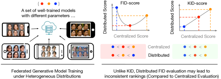
Figure 1: Centralized (score-all) vs. distributed (score-avg) evaluation of generative models. The centralized and distributed FID-based evaluations can lead to different rankings, while we prove the KID-based evaluations result in the same ranking.

In this work, we focus on the evaluation of deep generative models in heterogeneous distributed learning settings. Our primary goal is to highlight the challenges of extending standard evaluation metrics for generative models from the centralized setting to the heterogeneous distributed case. To do this, we consider and analyze the following two sensible extensions of an evaluation score: 1) the average score over clients (score-avg), i.e. the mean of the evaluation scores for individual clients, 2) the score with respect to the aggregate distribution of all clients (score-all) considering all the samples in the network. We consider standard assessment scores and analyze the consistency of model rankings suggested by the described extensions of the score to the distributed learning problem.

While the described score-all aggregation has been commonly used for the evaluation of generative models in the existing literature on distributed and federated generative model learning, we note that the estimation of the score-all metric will be challenging in a real distributed learning scenario. These challenges are mainly due to the privacy and computation constraints in standard distributed learning problems, preventing clients from sharing their observed samples and any revealing statistics of their training data with the rest of the network. On the other hand, the score-avg can be computed more efficiently since it only requires the client-based score value, which needs minor information on the samples and low communication expenses. However, it remains unclear if the original ranking of generative models according to score-all would be preserved under the score-avg assessment, because standard distances used for the evaluation task are non-linear in the input distributions.

In our theoretical analysis, we specifically focus on the Fréchet inception distance (FID) [9] and kernel inception distance (KID) [1] scores, which have been widely used in the evaluation of generative models. For the FID score, not only do we prove that the FID-all and FID-avg take different values, but further we show that the model rankings according to the two scores can be different. Indeed, we prove that the generative models with the optimal FID-avg and FID-all scores are different under heterogeneous client distributions, revealing the discrepancy between the two aggregate assessments.

On the other hand, in the case of KID score we prove that the aggregate scores KID-all and KID-avg result in the same rankings of generative models although they could take different values. This result shows the consistency of the KID evaluation between the mean aggregation in KID-avg and the collective data-based aggregation in KID-all. Therefore, our theoretical results suggest the different consistency behaviors of FID and KID scores when aggregated over a heterogeneous distributed learning setting: while averaging individual KID scores results in the same ranking as the KID score with respect to the distribution of collective client’s data, the same conclusion does not hold for FID and more generally Wasserstein distance-based evaluation metrics.

Finally, we discuss several numerical results on standard image datasets and generative model architectures which support our theoretical comparison of the aggregate evaluation scores in federated learning problems. Our empirical results suggest that the FID-all and FID-avg aggregations could lead to inconsistent rankings of the trained generative models in standard GANs and diffusion models. In our experiments, we observed that FID-avg often takes higher values when generated samples look sharper. On the other hand, the FID-all score seemed to be higher scores for models with higher diversity in their generated samples. In contrast, KID-all and KID-avg resulted in consistent rankings of the trained models where the evaluated score seems to aggregate both quality and diversity performance. In our numerical experiments, we also evaluated the precision, recall [22, 15], density, and coverage [17] scores under the two introduced aggregations which, except in the case of recall score, could lead to different rankings of the trained model under the discussed score aggregations. In the following, we summarize the main contributions of our study:

• Highlighting the challenges of evaluating generative models in heterogeneous distributed learning settings;

• Analyzing two types of aggregate FID scores in distributed learning scenarios and proving the inconsistencies between the optimal models under the two scores;

• Demonstrating the consistent rankings suggested by the client-wise averaged KID and the aggregate-data-based KID evaluations;

• Presenting numerical results on the evaluation of generative models in distributed settings and empirically supporting the theoretical claims.

2 Related Work

A large body of related works [26] has focused on the evaluation of generative models in standard centralized learning settings. The existing evaluation scores can be categorized into two general groups: 1) Distance-based metrics defining a distance between the distribution of training data and learnt generative model. The distance between the real and fake distributions is usually computed after passing the samples through a pre-trained neural net offering a proper embedding of image data. The well-known evaluation scores in this category are the FID [9] and KID [1] scores. 2) Quality and diversity-based scores which output a score based on the sharpness and variety of the generated samples. The widely-used evaluation metrics in this category are the Inception score [23], precision and recall metrics [22, 15], and density and coverage scores [17]. We note that in this work our goal is not to introduce a new evaluation metric, and our aim is to analyze the extensions of these scores to distributed and federated learning problems under heterogeneous data distributions across clients.

In another set of related works, extensions of generative model training methods including GANs and diffusion models to distributed federated learning have been studied. [20] propose Fed-GAN to train GANs in a federated learning setting. In [8], the gradient from sample generation for the generator is exchanged on the server, while each client possesses a personalized discriminator. According to [29], different weights are assigned to local discriminators in the non-i.i.d. setting. Conversely, [28] ensure client privacy by sharing the discriminator across clients, while keeping the generator private. Additionally, [25] explore a dual diffusion paradigm to extend diffusion-based models into the federated learning setting, addressing concerns related to data leakage.

3 Preliminaries

3.1 Deep Generative Models

In a deep generative model framework, a neural network generator $G$ is used to map a hidden random vector $\mathbf{Z}\in\mathbb{R}^{d}$ drawn according to a fixed distribution, e.g. isotropic multivariate Gaussian $\mathcal{N}(\mathbf{0},\sigma^{2}I)$ to a real-like sample $G(\mathbf{Z})$. Several deep learning approaches have been proposed to train such a generator network, including maximum-likelihood-based methods such as variational autoencoder [13] and flow-based models [5], generative adversarial networks (GANs) [6], and denoising diffusion models [10]. In our numerical evaluation, we mainly concentrated on the latter two methods, GANs and diffusion models, due to their state-of-the-art performance in computer vision applications.

In GANs, the training of generative models is framed as a min-max game between a generator network $G$ mapping latent vector $\mathbf{Z}$ to a real-like output and a discriminator network $D$ attempting to differentiate $G$’s generated samples from real training data. The GAN game is typically formulated as the following min-max optimization problem where $\bm{\theta},\,\bm{\omega}$ represent the parameters of generator and discriminator neural nets, and $f\bigl{(}G_{\bm{\theta}},D_{\bm{\omega}}\bigr{)}$ is the min-max objective representing $D$’s dissimilarity score for the generated and real samples:

$$\min_{\bm{\theta}}\;\max_{\bm{\omega}}\;f\bigl{(}G_{\bm{\theta}},D_{\bm{\omega}}\bigr{)}.$$ (1)

The training of GANs in a distributed learning problem aims at solving the above problem via a distributed optimization method. For example, in a federated learning setting where the local clients are connected to a single server node, the training of GAN players can be achieved by a federated min-max optimization algorithm as discussed in the related work section.

In the case of diffusion models, the generative model performs by multi-step denoising of a Gaussian input. The training of this approach is typically done by reversing the denoising process where the training data are turned to a Gaussian input via an iterative addition of independent Gaussian noise vectors. To extend diffusion models in federated learning, we follow the simple FedAvg [16] method and average the locally updated diffusion networks at the server followed by synchronizing the clients with the averaged model.

3.2 Distance-based Evaluation of Generative Models

In order to assess the performance of a generative model, a standard approach is to measure the distance between the distribution of real and generated data. Due to the high-dimensionality of standard image data, the evaluation of image-based generative models is typically performed after passing the data point through a pre-trained Inception model on the ImageNet dataset.

Specifically, a standard distance-based metric is the Fréchet inception distance (FID) defined as the $2$-Wasserstein distance between two Gaussian distributions with the mean and covariance parameters of the data distribution $P_{X}$, denoted by $\bm{\mu}_{X},C_{X}$, and with the mean and covariance of the generative model $P_{G}$, denoted by $\bm{\mu}_{G},C_{G}$:

$$\mathrm{FID}(P_{X},P_{G})\>:=\> \bigl{\|}\bm{\mu}_{X}-\bm{\mu}_{G}\bigr{\|}^{2}_{2}$$

$$\>+\mathrm{Tr}\Bigl{(}C_{X}+C_{G}-2\bigl{(}C_{X}C_{G}\bigr{)}^{1/2}\Bigr{)}.$$

Note that we can interpret the FID score as an approximation of the 2-Wasserstein distance given the first and second-order moments of the distributions.

Another widely-used distance-based score for the evaluation of generative models is the kernel inception distance (KID), which measures the maximum mean discrepancy (MMD) between the two distributions which is calculated using a kernel similarity function $k:\mathbb{R}^{d}\times\mathbb{R}^{d}\rightarrow\mathbb{R}$. Here, the definition of the MMD distance between $P_{X}$ and $P_{G}$ based on kernel $k$ follows from

$$\;\mathrm{KID}\bigl{(}P_{X},P_{G}\bigr{)}:=\;$$

$$\sup_{\begin{subarray}{c}f\in\mathcal{H}_{k}:\,\|f\|_{\mathcal{H}_{k}}\leq 1\end{subarray}}\Bigl{(}\mathbb{E}_{X\sim P_{X}}\bigl{[}f(X)\bigr{]}-\mathbb{E}_{X^{\prime}\sim P_{G}}\bigl{[}f(X^{\prime})\bigr{]}\Bigr{)}^{2}$$

In the above, $\mathcal{H}_{k}$ represents the reproducing kernel Hilbert space (RKHS) corresponding to kernel $k$, i.e., the function set that can be expressed by linear combination of kernel-based elements $k_{x}(\cdot)=k({x},\cdot)$ over $x\in\mathcal{X}$, and $\|\cdot\|_{\mathcal{H}_{k}}$ denotes the norm of this Hilbert space of functions.

3.3 Generative Model

3.4 Evaluating Generative Model

The definition of Distance-All and Distance-Avg

3.5 The Fairness in Federated Learning with Non-IID setting

The definition of normalized alpha-fairness for comparison between model with different ability.

4 Evaluation of Generative Models in Distributed Learning Settings

In this section, we discuss two extensions of distance-based evaluation scores from a centralized case to heterogeneous distributed learning settings. In our analysis, we use $\mathcal{D}(P_{X},P_{G})$ to denote a general distance between data distribution $P_{X}$ and the generative model $P_{G}$. For example, $\mathcal{D}$ can be chosen to be the FID score or KID score, which we will analyze later in the section.

In a standard centralized setting, we have only a single distribution $P_{X}$ for real data. However, the main characteristic of a heterogeneous distributed learning problem is the multiplicity of the involved clients’ distribution. Here, we suppose a distributed setting $k$ clients and use $P_{X_{1}},\ldots,P_{X_{k}}$ to denote their underlying distributions, i.e. $P_{X_{i}}$ stands for the data distribution at client $i$. In addition, we assume that every client $i$ contributes a fraction $0<\lambda_{i}<1$ of the data in the network, that is $\lambda_{i}=\frac{n_{i}}{n}$ with $n=\sum_{j=1}^{k}n_{j}$ is the total number of samples in the network and $n_{i}$ is the number of samples at client $i$.

As a result of multiple input distributions, we need to define an aggregate evaluation score that is based on distance measure $\mathcal{D}$. The aggregate distance is supposed to summarize the performance of the generative model $P_{G}$ in only one score. To do this, we consider and analyze two reasonable ways of defining the aggregate score:

1. Average Score $\mathcal{D}_{\mathrm{avg}}$: The score-avg is the mean of the client’s individual distance measures, i.e.

   $$\mathcal{D}_{\mathrm{avg}}\Bigl{(}P_{X_{1}},\ldots,P_{X_{k}}\,;\,P_{G}\Bigr{)}\,:=\,\sum_{i=1}^{k}\lambda_{i}\mathcal{D}\bigl{(}P_{X_{i}},P_{G}\bigr{)}.$$ (2)

2. Collective-data-based Score $\mathcal{D}_{\mathrm{all}}$: The score-all with respect to the collective data of the clients is the distance between $P_{G}$ to the averaged distribution $\widehat{P}_{X}:=\sum_{i=1}^{k}\lambda_{i}P_{X_{i}}$:

   $$\mathcal{D}_{\mathrm{all}}\Bigl{(}P_{X_{1}},\ldots,P_{X_{k}}\,;\,P_{G}\Bigr{)}\,:=\,\mathcal{D}\Bigl{(}\widehat{P}_{X}\,,\,P_{G}\Bigr{)}.$$ (3)

In the above, note that $\sum_{i=1}^{k}\lambda_{i}P_{X_{i}}$ is indeed a mixture distribution with $k$ components $P_{X_{1}},\ldots,P_{X_{k}}$ with frequency weights $\lambda_{1},\ldots,\lambda_{k}$. To relate the above aggregate scores, we first observe that when $\mathcal{D}$ is a convex function of the input distributions, which applies to both FID and KID scores, the score-avg $\mathcal{D}_{\mathrm{avg}}$ will upper-bound the score-all $\mathcal{D}_{\mathrm{all}}$:

Observation 1.

If $\mathcal{D}(P_{X},P_{G})$ is a convex function of $P_{X}$, then

$$\mathcal{D}_{\mathrm{all}}\Bigl{(}P_{X_{1}},\ldots,P_{X_{k}}\,;\,P_{G}\Bigr{)}\leq\mathcal{D}_{\mathrm{avg}}\Bigl{(}P_{X_{1}},\ldots,P_{X_{k}}\,;\,P_{G}\Bigr{)}$$

Remark 1.

The convexity assumption on distance $D$ in the above observation applies to standard divergence scores, including Wasserstein distances, $f$-divergence measures, total variation distance, and the maximum mean discrepancy. Consequently, the result applies to the FID and KID scores.

While the mentioned observation shows how the two aggregate scores are compared with one another, it does not imply a monotonic relationship between $\mathcal{D}_{\mathrm{all}}\Bigl{(}P_{X_{1}},\ldots,P_{X_{k}}\,;\,P_{G}\Bigr{)}$ and $\mathcal{D}_{\mathrm{avg}}\Bigl{(}P_{X_{1}},\ldots,P_{X_{k}}\,;\,P_{G}\Bigr{)}$. Therefore, this observation does not provide a comparison of the ranking of generative models according to the two aggregate scores. In the following subsections, we study this question for the particular FID and KID scores.

4.1 Aggregate FID Scores in Distributed Learning

In the case of FID score, we utilize the formulation of FID as the 2-Wassesrtein-distance between the Gaussian-fitted model that leads to a Riemannian geometry. This observation results in the following theorem on FID-all and FID-avg aggregations. We defer the proofs to the Appendix.

Theorem 1.

Suppose that $P_{X_{1}},\ldots,P_{X_{k}}$ are the clients’ distributions with the mean parameters $\bm{\mu}_{1},\ldots,\bm{\mu}_{k}$ and covariance matrices $C_{1},\ldots,C_{k}$, respectively, in the semantic space of the Inception net. Then, the following holds for a generative model $P_{G}$ with mean $\bm{\mu}_{G}$ and covariance $C_{G}$.

1. For FID-all, if we define random $\widehat{X}$ with the average mean $\widehat{\bm{\mu}}=\sum_{i=1}^{k}\lambda_{i}\bm{\mu}_{i}$ and covariance matrix $\widehat{C}=\sum_{i=1}^{k}\lambda_{i}\bigl{(}C_{i}+\bm{\mu}_{i}\bm{\mu}_{i}^{\top}-\widehat{\bm{\mu}}\widehat{\bm{\mu}}^{\top}\bigr{)}$ in the Inception-based semantic space, we have

   $$\mathrm{FID}_{\mathrm{all}}\Bigl{(}P_{X_{1}},\ldots,P_{X_{k}}\,;\,P_{G}\Bigr{)}\,=\,\mathrm{FID}\bigl{(}P_{\widehat{X}},P_{G}\bigr{)}.$$ (4)

2. For FID-avg, if we define a random vector $\widetilde{X}$ with the average mean $\widehat{\bm{\mu}}=\sum_{i=1}^{k}\lambda_{i}\bm{\mu}_{i}$ and covariance matrix $\widetilde{C}$ as the unique solution to $\widetilde{C}=\sum_{i=1}^{k}\lambda_{i}\bigl{(}\widetilde{C}^{1/2}C_{i}\widetilde{C}^{1/2}\bigr{)}^{1/2}$ in the Inception-based semantic space we will have

   $$\mathrm{FID}_{\mathrm{avg}}\Bigl{(}P_{X_{1}},\ldots,P_{X_{k}}\,;\,P_{G}\Bigr{)}\,$$

   $$=\,\mathrm{FID}\bigl{(}P_{\widetilde{X}},P_{G}\bigr{)}+\sum_{i=1}^{k}\lambda_{i}\mathrm{FID}\bigl{(}P_{\widetilde{X}},P_{X_{i}}\bigr{)}.$$

   Thus, the FID-all as a function of $G$ is changing monotonically with $\mathrm{FID}\bigl{(}P_{\widetilde{X}},P_{G}\bigr{)}$ for defined $\widetilde{X}$.

Remark 2.

In Theorem 1, $\widetilde{C}$ follows from the Wasserstein barycenter of the Gaussian distributions and under the condition that $C_{1},\ldots,C_{k}$ commute, i.e. $C_{i}C_{j}=C_{j}C_{i}$ for every $i,j$, simplifies to

$$\widetilde{C}=\Bigl{(}\sum_{i=1}^{k}\lambda_{i}C_{i}^{{1}/{2}}\Bigr{)}^{2}.$$

Remark 3.

In Theorem 1, the optimal mean vectors for FID-all and FID-avg aggregations are the same. In contrast, the optimal covariance matrix of FID-avg denoted by $\widetilde{C}$ has no dependence on the choice of $\bm{\mu}_{i}$’s, while the optimal covariance matrix of FID-all $\widetilde{C}$ will be affected by the difference between $\bm{\mu}_{i}$’s due to the term $\sum_{i=1}^{k}\lambda_{i}(\bm{\mu}_{i}\bm{\mu}_{i}^{\top}-\widehat{\bm{\mu}}\widehat{\bm{\mu}}^{\top})$. In general, Theorem 1 implies that the gap between FID-all and FID-avg can be written in the following form where $\mathrm{const.}$ remains constant under different $P_{G}$’s and $C_{G}$ is the embedded covariance matrix of $P_{G}$:

$$\mathrm{FID}_{\mathrm{avg}}\bigl{(}P_{X_{1}},\ldots,P_{X_{k}};P_{G}\bigr{)}-\mathrm{FID}_{\mathrm{all}}\bigl{(}P_{X_{1}},\ldots,P_{X_{k}};P_{G}\bigr{)}\>$$

$$=\>2\mathrm{Tr}\bigl{(}(C_{G}\widehat{C})^{1/2}-(C_{G}\widetilde{C})^{1/2}\bigr{)}\,+\,\mathrm{const.}$$

As explained in the remarks, Theorem 1 shows that the optimal covariance matrices under FID-all and FID-avg could be significantly different in heterogeneous settings with different $\bm{\mu}_{i}$’s. Therefore, since the FID-all and FID-avg scores can be interpreted as the distance to covariance matrices $\widehat{C}$ and $\widetilde{C}$, respectively, the rankings suggested by the aggregations will be different if two generators’ covariances $C_{G}$ and $C_{G^{\prime}}$ have different ordering of distances to $\widehat{C}$ and $\widetilde{C}$.

4.2 KID-based Evaluation in Distributed Learning

After showing the possibility of inconsistent rankings by FID-all and FID-avg, we consider the KID score and analyze the consistency of KID-all and KID-avg aggregations. The following theorem proves that unlike the FID-case, the KID-all and KID-avg will result in a consistent ordering of the models and there is a monotonic relationship between the two aggregate scores.

Theorem 2.

Consider a kernel function $k:\mathbb{R}^{d}\times\mathbb{R}^{d}\rightarrow\mathbb{R}$ and the resulting KID score. Then for the clients’ distributions $P_{X_{1}},\ldots,P_{X_{k}}$ with frequency parameters $\lambda_{1},\ldots,\lambda_{k}$, we will have the following for the average distribution $\widehat{P}_{X}=\sum_{j=1}^{k}\lambda_{j}P_{X_{j}}$:

$$\mathrm{KID}_{\mathrm{avg}}\Bigl{(}P_{X_{1}},\ldots,P_{X_{k}}\,;\,P_{G}\Bigr{)}\,$$

$$=\,\mathrm{KID}_{\mathrm{all}}\Bigl{(}P_{X_{1}},\ldots,P_{X_{k}}\,;\,P_{G}\Bigr{)}+\sum_{i=1}^{k}\lambda_{i}\,\mathrm{KID}\bigl{(}\widehat{P}_{X},P_{X_{i}}\bigr{)},$$

which implies a monotonic relationship between KID-all and KID-avg as a function of $P_{G}$.

Therefore, the above theorem shows the consistent rankings implied by the aggregate KID-avg and KID-all scores, as the difference between the scores remains constant while changing the model $P_{G}$.

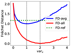
(a)

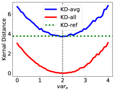
(b)

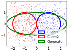
(c)

Figure 2: Experimental results of Gaussian mixture dataset. (a): The optimal $\mathrm{var}_{x}$ parameters are different under FD-avg and FD-all evaluations. (b): Distance between KD-avg and KD-all remains the same.(c): the clients’ and generator’s samples.

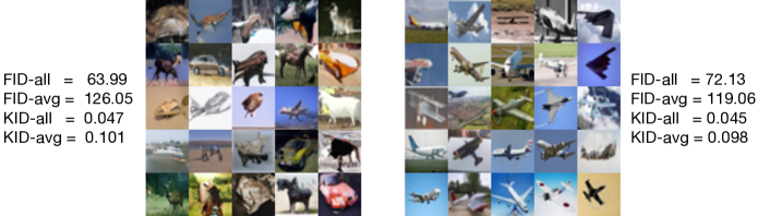
Figure 3: Left: Images generated by a generative model obtain a lower FID-all. Right: Images from real datasets with class ’airplane’ obtain a lower FID-avg. FID-avg and FID-all lead to inconsistent rankings, while KID-avg and KID-all result in the same ranking.

5 Numerical Results

5.1 Evaluation on Synthetic Gaussian Mixture Datasets

As discussed in Remark 3, the optimal selection of the covariance matrix differs for the FID-all and FID-avg aggregate scores. To illustrate this distinction, we performed a toy experiment, revealing that FID-avg attains its minimum value when the generator’s variance closely approximates that of an individual client, whereas FID-all is minimized when the variance equals that of the aggregate distribution.

Setup. Our experimental setup involves two clients, denoted by $C_{1}$ and $C_{2}$. $C_{1}$ possesses a dataset consisting of 50,000 samples drawn from the Gaussian distribution $\mathcal{N}([1,0]^{\top},\bm{\Sigma})$, while $C_{2}$ holds a dataset with 50,000 samples drawn from $\mathcal{N}([-1,0]^{\top},\bm{\Sigma})$, where $\bm{\Sigma}=\text{diag}([1,1]^{T})$. We introduce a generator, denoted as $G_{\mathrm{var}_{x}}$, which is parameterized by $\mathrm{var}_{x}$. $\mathrm{var}_{x}$ regulates the variance of the generator along the X-axis. Specifically, $G_{\mathrm{var}_{x}}$ generates 50,000 data points following a Gaussian distribution $\mathcal{N}([0,0]^{T},\bm{\Sigma_{G}})$, where $\bm{\Sigma_{G}}=\text{diag}([\mathrm{var}_{x},1]^{T})$. The relationship between the two clients and the generator is visually depicted in Figure 2. Additionally, we introduce an "ideal estimator" denoted as $\hat{E}=C_{1}\cup C_{2}$. This ideal estimator possesses the unique ability to replicate the distribution of the training dataset perfectly. We employ the ideal estimator as a reference for our analysis.

Evaluation Metrics. We measure the similarity between samples generated by clients and generators using the Fréchet distance (FD), which follows from the Wasserstein-based definition of FID-all and FID-avg without the application of the pre-trained Inception network. We consider the aggregate scores FD-avg and FD-all as defined in Equation 2 and Equation 3. Note that the FD-all for the ideal estimator is zero and we use $\text{\rm FD-ref}=\frac{1}{2}\sum_{i=1}^{2}\text{\rm FD}(\hat{E},C_{i})$ as a reference for FD-avg. We also measure the Kernel distance (KD), which follows the definition of KID-all and KID-avg without Inception network. KD-ref is defined for the kernel distance in a similar fashion to FD-ref.

Results. By increasing $\mathrm{var}_{x}$ from 0 to 4, we get a sequence of FD-avg / FD-all pairs and we plot them with the $\mathrm{var}_{x}$ in Figure 2. Our experimental results highlight the following conclusions. First, we observed that the minimum of FD-all occurs at $\mathrm{var}_{x}=2$, while that of FD-avg occurs at $\mathrm{var}_{x}=1$, which indicates that the optimal solutions of $\mathrm{var}_{x}$ to minimize FD-all and FD-avg are inconsistent. In this case, FD-all and FD-avg lead to different rankings of the models with $\mathrm{var}_{x}=1$ and $\mathrm{var}_{x}=2$. Additionally, we observed that, counterintuitively, the ‘ideal estimator’ did not reach the minimum average of the Fréchet distances. The distance between KD-avg and KD-all remains the same with the change of $\mathrm{var}_{x}$ and both of which reach minimum at $\mathrm{var}_{x}=2$. The toy experiment highlights how a co-variance mismatch between clients and the collective dataset leads to inconsistent rankings according to aggregate Fréchet distances.

5.2 Evaluation on Real Image Datasets

We evaluated our theoretical results on standard image datasets. In our experiments, we simulated heterogeneous federated learning experiments consisting of non-i.i.d. data at different clients: for CIFAR-10 [14], we considered 10 clients, each owning 5000 samples exclusively from a single class of the image dataset. Therefore, every client’s dataset contains 5000 images having the same label. We put the experiment on CIFAR-100 and ImageNet-32 [4, 3] in Appendix.

Neural Net-based Generators. We trained a DDPM models using the standard training protocols outlined in [10] under the federated CIFAR-10 setting described above. To train the generative models in the federated learning setting, we employed the standard FedAvg approach [16]. Detailed information regarding the experiment setting can be found in the Appendix.

Perfect Data-simulating Generators. In our CIFAR-10 experiments, we also simulated and evaluated an "ideal generator" capable of perfectly replicating all samples belonging to the ’airplane’ class in CIFAR10. In this scenario, the samples "generated" by the ideal generator exhibit impeccable fidelity but lack diversity since no samples from other categories can be produced.

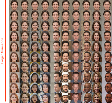
Figure 4: Illustration of randomly-generated samples from the variance-controlled generators. Images in each row are synthesized with the same truncation parameter.

(a) Client 1

(b) Client 2

(c) Client 3

(d) Client 4

(e) Client 5

(f) Client 6

Figure 5: Illustration of random samples from randomly selected variance-limited clients.

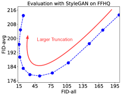
(a) FID-scores

(b) KID-scores

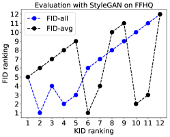
(c) Ranking

Figure 6: Evaluation on FFHQ with StyleGAN.

FID-based and KID-based Evaluation of Generative Models. We evaluated the generative models according to FID-all, FID-avg, KID-all, and KID-avg as defined in Section 4. In several cases, we observed that FID-all / FID-avg could assign inconsistent rankings to the generators. Specifically, we computed FID-all and FID-avg for the ideal ’airplane’-class-based generator and neural net-based DDPM generators under the distributed CIFAR10 setting. We present some examples generated from the two generators in Figure 3 and report their scores according to the four metrics. The results suggest that FID-avg assigns a considerably higher score to the ideal ’airplane’-based generator, whose images preserve perfect details but lack diversity in image categories. Conversely, FID-all assigns a relatively higher value to the DDPM model because its images possess greater diversity. On the other hand, we also observed that KID-avg and KID-all give consistent rankings. Both of them led to the evaluation that the ideal plane generator is slightly better than the DDPM generator. In our implementation of KID-scores, we utilized the standard implementation of KID measurement from data with a polynomial kernel, $k(\bf{x},\bf{y})=\left(\frac{1}{d}\bf{x}^{T}\bf{y}+1\right)^{3}$, where $d$ is the dimension of feature vector. We note that our theoretical finding on the evaluation consistency under KID-all and KID-avg applies to every kernel similarity function. We also test KID-scores with a Gaussian RBF kernel $k_{\sigma}^{\text{rbf}}(\bf{x},\bf{y})=\exp\left(-\frac{1}{2\sigma^{2}}\|\bf{x}-\bf{y}\|^{2}\right)$ as formulated in [1], where we chose $\sigma=\sqrt{d}$ in the experiments. For images generated by diffusion model $\text{KID}^{\text{rbf}}$-all gives $4.277e^{-3}$ while $\text{KID}^{\text{rbf}}$-avg gives $4.295e^{-3}$. And for the airplane images in CIFAR10, $\text{KID}^{\text{rbf}}$-all gives $4.283e^{-3}$ while $\text{KID}^{\text{rbf}}$-avg gives $4.301e^{-3}$. The results indicate that for Gaussian RBF kernel $k_{\sigma}^{\text{rbf}}$, $\text{KID}^{\text{rbf}}$-all and $\text{KID}^{\text{rbf}}$-avg still gives consistent results. In this case, the $\text{KID}^{\text{rbf}}$-based evaluation suggests the images sampled from the diffusion model have higher quality than the set of airplane images in the CIFAR10 dataset.

Figure 7: Precision / Recall and Density / Coverage under variance-limited federated CIFAR10.

5.3 Evaluation of Well-Trained Generators in Distributed Learning Contexts

Here, we extend our numerical analysis to a federated learning scenario with realistic generators. We use the widely used StyleGAN2-ADA[12] generator, and download an FFHQ pre-trained model weight from the StyleGAN2-ADA’s GitHub repository. The generated images have the size $1024\times 1024$. We synthesized a sequence of variance-controlled generators by applying the standard truncation technique [15] on the random noise $\bf{z}$. The truncation parameter $\tau$ varies from $0.01$ to $1.0$. A greater truncation parameter $\tau$ leads to higher diversity in generated samples. We illustrate how the truncation parameter affects the samples in Figure 4. For each truncation $\tau$, we generate 5000 samples from the model for the evaluation. Within each client, we repeat the style vectors for the last eight layers in StyleGAN to get better visualization results, which will not affect the conclusion.

Furthermore, to simulate a distributed learning setting where each client only possesses a small set of variance-limited samples, we synthesized 100 clients. Each of the clients hold 100 images synthesized by the model with truncation $\tau=0.25$. The centre vector of each clients are various. The images within each client look similar, while images across clients look highly different as shown in Figure 5.

Similarly, we evaluate the models based on the two aggregations of FID and KID scores in this setting. The numerical results are shown in Figure 6a and Figure 6b. The FID-avg vs. FID-all plot leads to a U-shape curve, while the gap between KID-avg and KID-all remains constant for different generators. We further show the relation between the ranking based on FID and KID aggregate scores in Figure 6c

5.4 Precision/Recall and Density/Coverege Evaluations

In addition to FID and KID, we followed the definition in Equation 2 and Equation 3 and performed similar experiments to evaluate the consistency between the two aggregate scores for Precision/Recall [15] and Density/Coverage [17]. In the case of Precision/Recall, we utilized the official implementation with the number of clusters set to 5. We assessed precision and recall under the variance-limited CIFAR10 setting, with the results presented in Figure 7. The numerical scores indicate that in a heterogeneous data setting, the two aggregate precision scores may not consistently rank the generative models. On the other hand, based on the recall’s definition, it can be seen that Recall-all and Recall-avg will always take the same value, since the recall score reduces to an average over the generated data. Our numerical results are also consistent with this observation. For the Density/Coverage evaluations, the numerical results in Figure 7 suggest that while the density-based aggregate scores lead to more consistent rankings under data heterogeneity, both density-all/-avg may still provide inconsistent rankings. On the other hand, the coverage-based evaluations mimic the recall-based evaluation and consistently rank the models.

6 Conclusion

In this paper, we studied the evaluation of generative models in heterogeneous distributed learning problems where the clients have different distributions. We discussed the challenges of evaluating the overall performance of a trained generative model with only one score and showed the inconsistent rankings of sensible aggregations of standard FID scores in the network. On the other hand, we demonstrated that the same extensions of KID offer the same ranking of generative models. Our theoretical and experimental results indicate that KID-avg can be computed efficiently under the privacy constraints in distributed learning problems, while preserving the KID-all-based ranking of generative models. A possible future direction for our work is to extend the theoretical study to other evaluation criteria such as precision/recall and density/coverage scores. Also, understanding the behavior of the aggregate score using non-arithmetic averaging could be useful for evaluating deep generative models in federated learning contexts.

Limitations and Broader Impact

We note that our numerical study focuses on the applications of generative models to image datasets and the empirical conclusions may not apply to other standard types of data including text and audio data. Regarding the work’s broader impact, we note that our analysis could be connected to the fairness evaluation of generative models in distributed learning contexts, as it suggests evaluation metrics for the assessment of diversity in the generated data. The study of fairness and diversity for generative models is required for a principled deployment of generative models in sensitive machine learning applications.

Appendix A Proofs

A.1 Proof of Theorem 1

1. Note that according to the definition,

   $$\mathrm{FID}_{\mathrm{all}}\Bigl{(}P_{X_{1}},\ldots,P_{X_{k}}\,;\,P_{G}\Bigr{)}\,=\,\mathrm{FID}\bigl{(}\sum_{i=1}^{k}\lambda_{i}P_{X_{i}},P_{G}\bigr{)}.$$

   Since the FID score depends only on the the mean and covariance parameters in the Inception-based semantic space, we can replace $\sum_{i=1}^{k}\lambda_{i}P_{X_{i}}$ with any other distribution that shares the same mean and covariance parameters, and the FID value will not change. Observe that given mean parameters $\bm{\mu}_{1},\ldots,\bm{\mu}_{k}$, the Inception-based mean of $\sum_{i=1}^{k}\lambda_{i}P_{X_{i}}$ will be $\widehat{\bm{\mu}}=\sum_{i=1}^{k}\lambda_{i}\bm{\mu}_{i}$. Therefore, the Inception-based covariance matrix of $\sum_{i=1}^{k}\lambda_{i}P_{X_{i}}$ follows from

   $$\sum_{i=1}^{k}\lambda_{i}\mathbb{E}_{P_{i}}\bigl{[}\bigl{(}X_{i}-\widehat{\bm{\mu}}\bigr{)}\bigl{(}X_{i}-\widehat{\bm{\mu}}\bigr{)}^{\top}\bigr{]}\> =\>\sum_{i=1}^{k}\lambda_{i}\Bigl{[}C_{i}+\bigl{(}\bm{\mu}_{i}-\widehat{\bm{\mu}}\bigr{)}\bigl{(}\bm{\mu}_{i}-\widehat{\bm{\mu}}\bigr{)}^{\top}\Bigr{]}$$

   $$=\>\sum_{i=1}^{k}\lambda_{i}\Bigl{[}C_{i}+\bm{\mu}_{i}\bm{\mu}_{i}^{\top}\Bigr{]}-\widehat{\bm{\mu}}\widehat{\bm{\mu}}^{\top}$$

   $$=\>\widehat{C}.$$

   Therefore, since we assume $\widehat{X}$ has the Inception-based mean and covariance $\widehat{\bm{\mu}}$ and $\widehat{C}$, the proof of this part is complete.

2. According to the definition, FID-avg can be written as

   $$\mathrm{FID}_{\mathrm{avg}}\Bigl{(}P_{X_{1}},\ldots,P_{X_{k}}\,;\,P_{G}\Bigr{)}\,\>:=\>\sum_{i=1}^{k}\lambda_{i}\mathrm{FID}\bigl{(}P_{X_{i}},P_{G}\bigr{)}.$$

   Therefore, we have

   $$\mathrm{FID}_{\mathrm{avg}}\Bigl{(}P_{X_{1}},\ldots,P_{X_{k}}\,;\,P_{G}\Bigr{)}\,$$

   $$\stackrel{{\scriptstyle(a)}}{{=}}\> \sum_{i=1}^{k}\lambda_{i}W^{2}_{2}\Bigl{(}\mathcal{N}(\bm{\mu}_{i},C_{i}),\mathcal{N}(\bm{\mu}_{G},C_{G})\Bigr{)}$$

   $$\stackrel{{\scriptstyle(b)}}{{=}}\> \sum_{i=1}^{k}\lambda_{i}\Bigl{[}\|\bm{\mu}_{i}-\bm{\mu}_{G}\|^{2}_{2}+\mathrm{Tr}\bigl{(}C_{i}+C_{G}-(C_{i}C_{G})^{1/2}\bigr{)}\Bigr{]}$$

   $$=\> \sum_{i=1}^{k}\Bigl{[}\lambda_{i}\|\bm{\mu}_{i}-\bm{\mu}_{G}\|^{2}_{2}\Bigr{]}+\sum_{i=1}^{k}\Bigl{[}\lambda_{i}\mathrm{Tr}\bigl{(}C_{i}+C_{G}-(C_{i}C_{G})^{1/2}\bigr{)}\Bigr{]}$$

   $$\stackrel{{\scriptstyle(c)}}{{=}}\> \|\widehat{\bm{\mu}}-\bm{\mu}_{G}\|^{2}_{2}+\sum_{i=1}^{k}\Bigl{[}\lambda_{i}\|\widehat{\bm{\mu}}-\bm{\mu}_{i}\|^{2}_{2}\Bigr{]}$$

   $$\qquad+\mathrm{Tr}\bigl{(}C_{G}+\widehat{C}-(C_{G}\widehat{C})^{1/2}\bigr{)}+\sum_{i=1}^{k}\Bigl{[}\lambda_{i}\mathrm{Tr}\bigl{(}C_{i}+\widehat{C}-(C_{i}\widehat{C})^{1/2}\bigr{)}\Bigr{]}$$

   $$=\> \|\widehat{\bm{\mu}}-\bm{\mu}_{G}\|^{2}_{2}+\mathrm{Tr}\bigl{(}C_{G}+\widehat{C}-(C_{G}\widehat{C})^{1/2}\bigr{)}$$

   $$\qquad+\sum_{i=1}^{k}\Bigl{[}\lambda_{i}\|\widehat{\bm{\mu}}-\bm{\mu}_{i}\|^{2}_{2}+\lambda_{i}\mathrm{Tr}\bigl{(}C_{i}+\widehat{C}-(C_{i}\widehat{C})^{1/2}\bigr{)}\Bigr{]}$$

   $$=\> \|\widehat{\bm{\mu}}-\bm{\mu}_{G}\|^{2}_{2}+\mathrm{Tr}\bigl{(}C_{G}+\widehat{C}-(C_{G}\widehat{C})^{1/2}\bigr{)}$$

   $$\qquad+\sum_{i=1}^{k}\lambda_{i}\Bigl{[}\|\widehat{\bm{\mu}}-\bm{\mu}_{i}\|^{2}_{2}+\mathrm{Tr}\bigl{(}C_{i}+\widehat{C}-(C_{i}\widehat{C})^{1/2}\bigr{)}\Bigr{]}$$

   $$\stackrel{{\scriptstyle(d)}}{{=}}\> \mathrm{FID}(P_{\widehat{X}},P_{G})+\sum_{i=1}^{k}\lambda_{i}\mathrm{FID}(P_{\widehat{X}},P_{X_{i}}).$$

   In the above, $(a)$ follows from the Wasserstein-based definition of FID distance. $(b)$ comes from the well-known closed-form expression of the 2-Wasserstein distance between Gaussian distributions [27]. $(c)$ is the result of applying the weighted barycenter of vector $\bm{\mu}_{1},\ldots,\bm{\mu}_{k}$ that can be seen to be $\widehat{\bm{\mu}}$ and the weighted barycenter of positive semi-definite covariance matrices $C_{1},\ldots,C_{k}$ that has been shown to be the unique matrix $\widehat{C}$ that solves the equation $\widetilde{C}=\sum_{i=1}^{k}\lambda_{i}\bigl{(}\widetilde{C}^{1/2}C_{i}\widetilde{C}^{1/2}\bigr{)}^{1/2}$ [21, 18]. $(d)$ is the direct consequence of the Wasserstein-based definition of the FID distance and the closed-form expression of the 2-Wasserstein distance between Gaussians. Therefore, the proof is complete.

A.2 Proof of Theorem 2

To show this theorem, we note that if $\phi(X)$ is the kernel feature map for kernel $k$ used to define the KID distance, i.e. $k(x,y)=\langle\phi(x),\phi(y)\rangle$ is the inner product of the feature maps applied to $x,y$, then it can be seen that the kernel-$k$-based MMD distance can be written as

$$\mathrm{MMD}\bigl{(}P_{X},P_{G}\bigr{)}:= \mathbb{E}_{X,X^{\prime}\sim P_{X}}\bigl{[}k(X,X^{\prime})\bigr{]}+\mathbb{E}_{Y,Y^{\prime}\sim P_{G}}\bigl{[}k(Y,Y^{\prime})\bigr{]}-2\,\mathbb{E}_{X\sim P_{X},\,Y\sim P_{G}}\bigl{[}k(X,Y)\bigr{]}$$

$$= \Bigl{\|}\mathbb{E}\bigl{[}\phi(X)\bigr{]}-\mathbb{E}\bigl{[}\phi(Y)\bigr{]}\Bigr{\|}^{2}.$$

Therefore, following the definition of KID-avg, we can write

$$\mathrm{KID}_{\mathrm{avg}}\Bigl{(}P_{X_{1}},\ldots,P_{X_{k}}\,;\,P_{G}\Bigr{)}\,\>:= \>\sum_{i=1}^{k}\lambda_{i}\mathrm{KID}\bigl{(}P_{X_{i}},P_{G}\bigr{)}$$

$$= \>\sum_{i=1}^{k}\lambda_{i}\mathrm{MMD}_{\phi}\bigl{(}P_{X_{i}},P_{G}\bigr{)}$$

$$\stackrel{{\scriptstyle(a)}}{{=}} \>\sum_{i=1}^{k}\lambda_{i}\Bigl{\|}\mathbb{E}\bigl{[}\phi(X_{i})\bigr{]}-\mathbb{E}\bigl{[}\phi(G(Z))\bigr{]}\Bigr{\|}^{2}$$

$$\stackrel{{\scriptstyle(b)}}{{=}} \>\bigl{\|}\mathbb{E}\bigl{[}\phi(\widehat{X})\bigr{]}-\mathbb{E}\bigl{[}\phi(G(Z))\bigr{]}\bigl{\|}^{2}+\sum_{i=1}^{k}\Bigl{[}\lambda_{i}\bigl{\|}\mathbb{E}\bigl{[}\phi(X_{i})\bigr{]}-\mathbb{E}\bigl{[}\phi(\widehat{X})\bigr{]}\bigr{\|}^{2}\Bigr{]}$$

$$\stackrel{{\scriptstyle(c)}}{{=}} \>\mathrm{MMD}_{\phi}\bigl{(}\widehat{P}_{X},P_{G}\bigr{)}+\sum_{i=1}^{k}\Bigl{[}\lambda_{i}\mathrm{MMD}_{\phi}\bigl{(}\widehat{P}_{X},P_{X_{i}}\bigr{)}\Bigr{]}$$

$$\stackrel{{\scriptstyle(d)}}{{=}} \>\mathrm{KID}\bigl{(}\widehat{P}_{X},P_{G}\bigr{)}+\sum_{i=1}^{k}\Bigl{[}\lambda_{i}\mathrm{KID}\bigl{(}\widehat{P}_{X},P_{X_{i}}\bigr{)}\Bigr{]}$$

$$\stackrel{{\scriptstyle(e)}}{{=}} \>\mathrm{KID}_{\mathrm{all}}\Bigl{(}P_{X_{1}},\ldots,P_{X_{k}}\,;\,P_{G}\Bigr{)}+\sum_{i=1}^{k}\lambda_{i}\mathrm{KID}\bigl{(}\widehat{P}_{X},P_{X_{i}}\bigr{)}.$$

In the above, $(a)$ and $(c)$ follow from the feature-map-based formulation of the MMD distance. $(b)$ is the consequence of the fact that $\|\cdot\|$ is the norm in a reproducing kernel Hilbert space and for $\widehat{X}$ distributed as $\widehat{P}_{X}=\sum_{i=1}^{k}\lambda P_{X_{i}}$ we know that $\mathbb{E}\bigl{[}\phi(\widehat{X})\bigr{]}$ is the weighted barycenter of the individual mean vectors $\mathbb{E}\bigl{[}\phi({X}_{1})\bigr{]},\ldots,\mathbb{E}\bigl{[}\phi({X}_{k})\bigr{]}$. $(d)$ is based on the definition of KID. Finally, $(e)$ follows from the definition of KID-all, which completes the proof.

Appendix B Details

We have trained WGAN-GP [23] and DDPM [10] in a federated learning setting by utilizing FedAvg approach [16]. The experiment protocols for WGAN-GP and DDPM are copied from original works. The communication interval of FedAvg is set as 160 iterations for both WGAN-GP and DDPM. We have tried different communication intervals for both models. The communication frequency will affect model performance but have no influence on the conclusions in the main part of our paper.

Appendix C General 1-Wasserstein-Distance evaluation Metrics

Let $\mathbb{P}_{g}$ and $\mathbb{P}_{t}$ represent the distribution of generated set and training set. The Wasserstain-1 distance between $\mathbb{P}_{g}$ and $\mathbb{P}_{t}$ is,

$$W(\mathbb{P}_{g},\mathbb{P}_{t})=\mathop{inf}\limits_{\lambda\in\Pi(\mathbb{P}_{g},\mathbb{P}_{t})}\mathbb{E}_{(x,y)\sim\lambda}[\|x-y\|],$$ (5)

where $\Pi(\mathbb{P}_{g},\mathbb{P}_{t})$ denotes the set of all joint distribution $\lambda(x,y)$ whose marginal distribution are respectively $\mathbb{P}_{g}$ and $\mathbb{P}_{t}$. However, the direct estimation of $W(\mathbb{P}_{g},\mathbb{P}_{t})$ is highly intractable. On the other hand, the Kantorovich-Rubinstein duality [27] gives,

$$W(\mathbb{P}_{g},\mathbb{P}_{t})=\mathop{sup}\limits_{\|f\|_{L}\leq 1}\mathbb{E}_{x\sim\mathbb{P}_{g}}[f(x)]-\mathbb{E}_{x\sim\mathbb{P}_{t}}[f(x)],$$ (6)

where the supremum is over all the 1-Lipschitz functions $f:\mathcal{R}^{n}\rightarrow\mathcal{R}$. Therefore, if we have a parameterized family of functions $\{f_{\theta}\}_{\theta\in\Theta}$ that a 1-Lipschitz, we could considering solve this problem,

$$\mathop{max}\limits_{\theta\in\Theta}\mathbb{E}_{x\sim\mathbb{P}_{g}}[f_{\theta}(x)]-\mathbb{E}_{x\sim\mathbb{P}_{t}}[f_{\theta}(x)].$$ (7)

To estimate the supremum of Equation 6, we employ a family of non-linear neural network $f_{\theta}$ which are repeatedly stacked by the fully connected layer, the spectral normalization and RELU activation layer. There are three repeated blocks in the network $f_{\theta}$ and the last block does have RELU. The feature is extracted by pre-trained Inception-V3 network. By optimizing the parameters in $f_{\theta}$ to maximize $\mathbb{E}_{x\sim\mathbb{P}_{g}}[f_{\theta}(x)]-\mathbb{E}_{x\sim\mathbb{P}_{t}}[f_{\theta}(x)]$ over $\mathbb{P}_{g}$ and $\mathbb{P}_{t}$, we can finally get an estimation of $W(\mathbb{P}_{g},\mathbb{P}_{t})$. And similarly, we can also define average score W-avg and collective-data-based score W-all under the distributed learning setting. Similar to the CIFAR100 experiment in the main body of paper, we extracted samples from each single class of CIFAR100 and evaluate these samples on federated CIFAR10 dataset. We illustrate a subset of W-avg / W-all pairs in Figure 8. According to experiment results, we find that general 1-Wasserstein-Distance evaluation metric also shows inconsistent behaviours in the distributed evaluation settings.

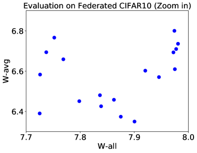
Figure 8: Evaluation with 1-Wasserstein-Distance on Federated CIFAR10.

Appendix D Evaluation of Synthetic Gaussian Mixture Data with the Log-Likelihood Score

We also evaluated the synthetic Gaussian mixture dataset mentioned in Section 5.1 with the standard log-likelihood (LL) score. In this experiment, we note that we have access to the probability density functions (PDF) of the simulated generator. We utilized the generator $G_{var_{x}}$ described in the main text and performed the evaluation over the parameter $\mathrm{var}_{x}$ in the range $[0,40]$. As can be shown in the general case, LL-avg and LL-all led to the same value for every evaluated model. As shown in Figure 9a, they reached their maximum value at $\mathrm{var}_{x}=2$. On the other hand, we set a new generator $G_{mean_{x}}$ generating samples according to $\mathcal{N}([\mathrm{mean}_{x},0]^{\top},\bm{\Sigma})$, where $\bm{\Sigma}=\text{diag}([2,1]^{T})$. We gradually increased $\mathrm{mean}_{x}$ from -2 to 2 and plotted LL-avg, LL-all, and LL-ref in Figure 9b.

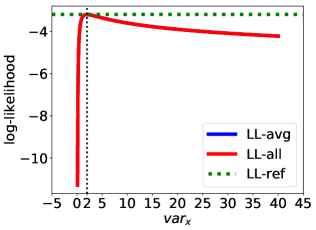
(a) $G_{var_{x}}$

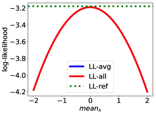
(b) $G_{mean_{x}}$

Figure 9: Evaluation of synthetic Gaussian data with the aggregate log-likelihood scores.

Appendix E Extra Experiment Results on Well-trained Generative Models

E.1 Extra samples from clients

We show more samples from clients described in Section 5.3 on Figure 10.

(a) Client 7

(b) Client 8

(c) Client 9

(d) Client 10

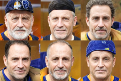
(e) Client 11

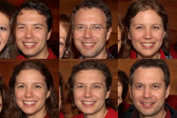
(f) Client 12

Figure 10: Illustration of random samples from randomly selected variance-limited clients.

E.2 Results on AFHQ dataset

Utilizing a another model weight that is pre-trained on AFHQ-wild dataset [2], we extend the experiment described in Section 5.3. Similar to the main text, we gradually increase the truncation parameter of generators We show some examples from generators, clients on Figure 12 and Figure 11 and plot the relationship between FID-scores and KID-scores on Figure 13. The results that are illustrated in the figures still indicates that FID-avg can lead to different ranking with FID-all, while KID-avg can be treated as a more stable evaluation metric in the distributed learning setting.

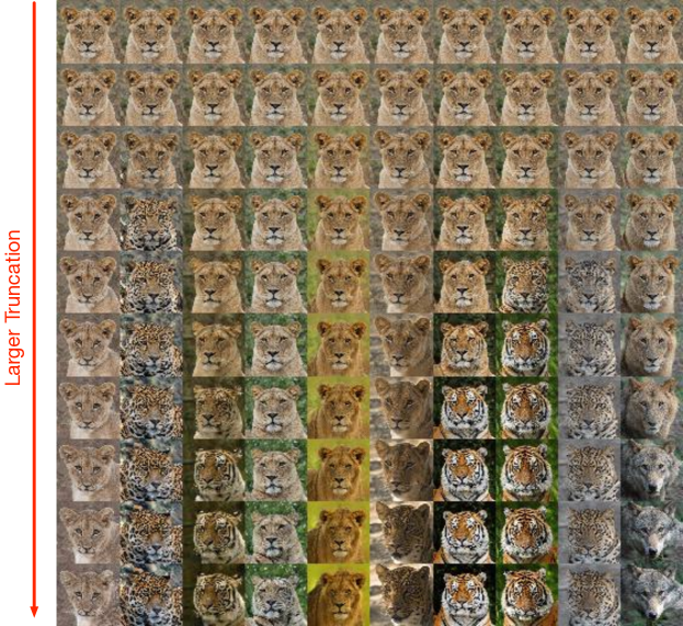
Figure 11: Illustration of randomly-generated samples from the variance-controlled generators on AFHQ dataset. Images in each row are synthesized with the same truncation parameter.

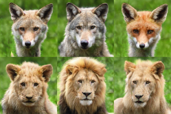
(a) Client 1

(b) Client 2

(c) Client 3

(d) Client 4

(e) Client 5

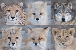
(f) Client 6

Figure 12: Illustration of random samples from randomly selected variance-limited clients on AFHQ dataset.

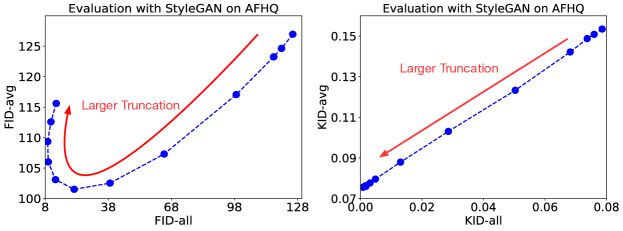
Figure 13: Evaluation on AFHQ dataset with StyleGAN2.

Appendix F Extra Experiment Results on Federated Datasets

Similar to the federated CIFAR10 in Section 5.2, federated CIFAR100 and federated ImageNet-32 are conducted by grouping samples from a each class. In this section, we report some extra numerical results that evaluated on the three federated image datasets.

F.1 Evaluate Sequence of Net-based Generator on Federated CIFAR10

We trained the WGAN-GP[7] generative models multiple times using different random states, and we set different training lengths for every training procedure. We saved the models at different checkpoints every $10$ epochs, which is common in training generative models to select the best-performing saved model according to an evaluation metric.

Our numerical results suggest that the gap between KID-all and KID-avg remains constant and hence they lead to the same rankings of the generative models. Here, we conducted our evaluations on all the generative models instances as previously described, and the results are visualized in the left sub-figure of Figure 14. These findings reveal that all distinct generators consistently exhibit a uniform gap between KID-avg and KID-all. Consequently, our results indicate that the rankings established by KID-avg consistently align with those of KID-all in distributed learning settings.

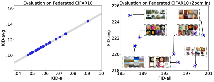
Figure 14: Left: KID evaluations of WGAN-GP checkpoints on federated CIFAR10. Right: FID-based evaluations on federated CIFAR-10.

F.2 Evaluate CIFAR100 Generator on Federated CIFAR10

To further experiment the ranking of generative models according to the discussed aggregate scores, we extracted samples from each class of CIFAR-100 and treated them as the output of one hundred distinct generators, each corresponding to a single class. By assessing these generators on the federated CIFAR-10 dataset, we obtained one hundred pairs of FID-avg / FID-all values, and a subset of these pairs with inconsistent rankings according to FID-all/FID-avg is visualized in the right of Figure 14. The complete set of evaluation results is available on Table 1. These results further highlight that the rankings provided by FID-all and FID-avg can exhibit inconsistencies in the context of distributed learning. Such inconsistencies could pose a challenge when selecting from a series of checkpoints or model architectures during the training of generative models in distributed learning scenarios, where a distributed computation of FID-all is more challenging than obtaining FID-avg due to privacy considerations.

Class	FID-all	FID-avg	KID-all	KID-avg	Class	FID-all	FID-avg	KID-all	KID-avg
0	267.4	285.9	0.201	0.253	25	142.4	173.2	0.067	0.116
1	173.2	205.5	0.109	0.165	26	139.4	175.5	0.063	0.114
2	151.8	185.4	0.072	0.123	27	114.5	153.7	0.054	0.102
3	124.3	162.2	0.047	0.100	28	182.0	205.0	0.112	0.160
4	117.0	156.1	0.049	0.100	29	143.3	185.2	0.083	0.133
5	157.6	185.2	0.088	0.138	30	147.4	179.8	0.084	0.134
6	142.1	179.7	0.062	0.115	31	160.4	193.6	0.108	0.158
7	144.9	179.2	0.066	0.113	32	115.4	156.4	0.032	0.085
8	155.0	187.7	0.085	0.135	33	146.9	181.2	0.077	0.126
9	180.7	203.6	0.106	0.156	34	127.5	163.4	0.068	0.117
10	183.2	208.8	0.099	0.151	35	150.4	184.7	0.080	0.131
11	151.9	184.9	0.073	0.127	36	142.5	176.5	0.070	0.126
12	126.1	163.1	0.056	0.108	37	126.7	162.9	0.066	0.118
13	127.0	159.4	0.058	0.112	38	110.5	151.3	0.050	0.100
14	145.8	182.9	0.071	0.126	39	233.5	257.2	0.145	0.196
15	124.2	165.2	0.054	0.107	40	158.9	187.6	0.078	0.128
16	190.3	213.6	0.112	0.161	41	151.1	181.0	0.072	0.126
17	161.5	192.8	0.117	0.165	42	137.2	174.7	0.071	0.122
18	142.7	179.8	0.069	0.118	43	152.0	186.0	0.090	0.139
19	112.4	154.1	0.047	0.101	44	126.7	165.8	0.050	0.103
20	194.2	215.9	0.123	0.175	45	135.4	173.0	0.059	0.111
21	164.8	194.9	0.099	0.148	46	155.1	187.1	0.080	0.133
22	205.1	227.0	0.126	0.180	47	174.2	203.4	0.118	0.169
23	191.1	219.7	0.130	0.186	48	145.0	175.3	0.077	0.129
24	174.9	202.8	0.105	0.155	49	164.8	194.6	0.110	0.164
50	113.8	154.0	0.045	0.095	75	151.7	184.3	0.096	0.145
51	150.4	184.6	0.073	0.125	76	151.5	183.5	0.068	0.118
52	195.3	222.1	0.167	0.218	77	139.0	174.9	0.066	0.117
53	279.7	299.1	0.217	0.270	78	197.3	228.3	0.130	0.182
54	170.2	201.3	0.098	0.149	79	138.9	174.8	0.062	0.114
55	104.7	146.3	0.034	0.086	80	111.1	149.9	0.043	0.095
56	144.2	178.5	0.075	0.126	81	131.7	165.3	0.068	0.119
57	192.5	219.9	0.115	0.163	82	197.6	227.2	0.123	0.178
58	131.5	161.0	0.067	0.121	83	202.6	230.6	0.122	0.173
59	149.7	183.7	0.093	0.144	84	144.5	177.3	0.065	0.111
60	188.0	216.0	0.144	0.197	85	123.0	160.7	0.079	0.125
61	249.2	270.6	0.179	0.229	86	168.0	193.0	0.083	0.135
62	202.1	230.6	0.133	0.184	87	170.5	196.0	0.098	0.152
63	140.6	175.3	0.071	0.120	88	133.4	170.6	0.068	0.120
64	118.7	156.1	0.049	0.100	89	122.3	158.1	0.059	0.112
65	102.2	142.2	0.024	0.077	90	110.7	148.3	0.041	0.093
66	121.7	159.1	0.054	0.105	91	124.0	160.7	0.048	0.098
67	132.5	167.8	0.063	0.115	92	175.4	206.2	0.096	0.149
68	139.7	173.1	0.073	0.123	93	129.7	166.3	0.054	0.109
69	143.2	176.0	0.068	0.121	94	213.4	235.2	0.162	0.212
70	178.4	209.5	0.095	0.148	95	154.7	185.2	0.084	0.133
71	169.4	199.0	0.120	0.167	96	147.8	181.7	0.090	0.138
72	114.1	155.6	0.043	0.094	97	137.1	171.4	0.068	0.119
73	137.9	170.8	0.071	0.124	98	157.1	188.6	0.082	0.134
74	124.7	162.1	0.061	0.108	99	204.9	233.9	0.143	0.192

Table 1: Full evaluation of CIFAR100 on Federated CIFAR10.

F.3 Evaluate CIFAR100 on Federated ImageNet-32

We expand the evaluation of CIFAR100 to Federated ImageNet-32 dataset. Similarly, we extracted samples from each class of CIFAR-100 and treated them as the output of one hundred distinct generators, each corresponding to a single class. We also keep the first one hundred classes of ImageNet-32 and simulate one hundred clients. Each client hold all images ($\sim$1300) from a single class. We evaluate all the generators on Federated ImageNet-32 and the result is shown in Figure 15. The ranks provided by FID-avg and FID-all is inconsistent in a much more complex distributed learning setting.

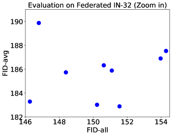
Figure 15: Evaluate CIFAR100 on Federated ImageNet-32.

Appendix G Extra Experiment Results on Variance-Limited Federated Dataset

In the federated learning literature, it is relatively common that each client possesses only a small portion of the collective dataset, and the data diversity within each client’s holdings is significantly constrained. To illustrate, consider the case of smartphone users who exclusively own pictures of themselves, all of which share remarkable similarity. Nevertheless, in a network comprising millions of users, the overall dataset’s distribution still exhibits significant variance. In such scenarios, our theoretical framework suggests that the disparity between FID-all and FID-avg can become more pronounced. To experiment the effect of such distribution heterogeneity, we simulated and evaluated generative models under variance-limited federated datasets. To obtain a variance-limited federated dataset, for each class in the image dataset, we kept only a single image and its K-nearest neighbors. To find the $K$ nearest neighbors, we used the $L_{2}$-distance in the Inception-V3 2048-dimensional semantic space. It is worth noting that our experimentation has shown that varying K within the range of 5 to 100 does not alter the core conclusions. This approach effectively mimics scenarios where each client’s data has limited variance. We simulated the variance-limited federated learning setting for CIFAR-10, CIFAR-100 and a 32$\times$32 version of ImageNet (IN-32). For CIFAR-10 and CIFAR-100, we utilized all the classes in the dataset and for IN-32 we utilized the first 100 classes. We chose $K=20$ in the experiments. Intuitively, a larger $K$ leads to a more significant intra-client variance.

Variance-controlled Generators. To simulate a generator, we initiate the process by randomly selecting a sample from the dataset. We then gather its M-nearest neighbors from the original dataset (w/o federated learning setting). We consider this subset of samples as a set of generated samples generated by a generator denoted by $G_{M}$. By increasing the value of $M$, we generated a sequence of generators with progressively higher variance values. We tried the $M$ range from 100 to 50000. We evaluated all the generative models, denoted as $G_{M}$ with the chosen $M$ values, using the Variance-Limited Federated datasets.

G.1 Results on Variance-Limited Federated CIFAR10

The evaluation results on CIFAR10 are shown in Figure 16. Our findings reveal a distinct pattern in the behavior of FID-avg and FID-all as generator variance varies while the distance between KID-avg and KID-all remains the same. Our numerical results highlight the impact of the choice of FID-all and FID-avg on model rankings in federated learning settings with limited intra-client variance. , which can be broadly categorized into three phases.

G.2 Results on Variance-Limited Federated CIFAR100

Similar to the experiments on CIFAR10, we have also applied the variance-limited federated dataset setting to CIFAR100. We keeps K=20 images in each class. For variance-controlled generators, we select a sample from original CIFAR100 and gather the M-nearset neighbors. The range of M keeps the same with that in the previous subsection. We show the results in Figure 17. The results still support our main claims: FID-avg and FID-all gives inconsistent results while KID-avg and KID-all give the same.

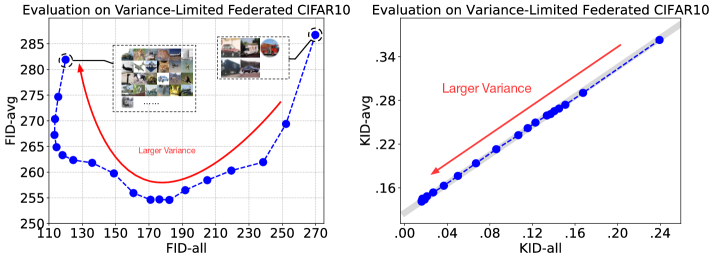
Figure 16: Left: KID evaluations of WGAN-GP checkpoints on federated CIFAR10. Right: FID-based evaluations on federated CIFAR-10.

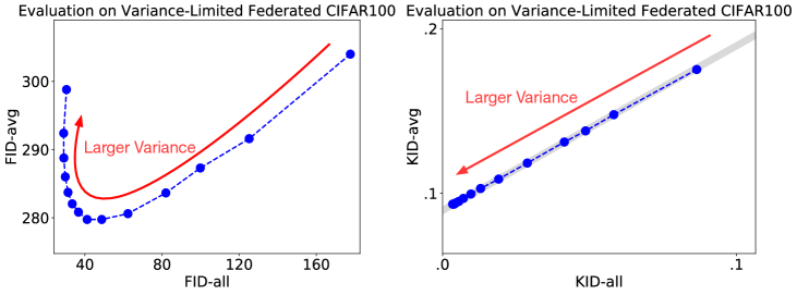
Figure 17: Evaluation on Variance-Limited Federated CIFAR100.

G.3 Results on Variance-Limited Federated IN32

Results on ImageNet-32 are illustrated in Figure 18. We further plot the relationship between ranking given by FID-scores and KID-scores in Figure 19.

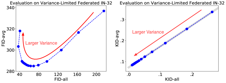
Figure 18: FID and KID-based Evaluations of variance-controlled generators on variance-limited federated ImageNet-32.

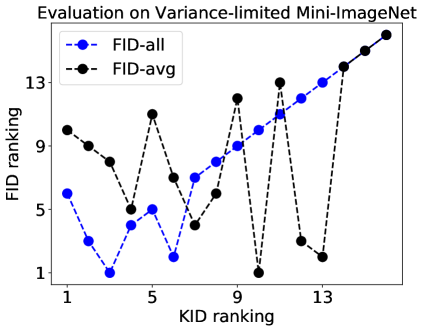
Figure 19: Comparing FID-based and KID-based rankings of variance-limited federated Mini-ImageNet-based simulated generative models. The lower the rank is, the better.

G.4 The Effect of Intra-Client Variance

In the main body of this paper, we choose $K=20$ when we conduct the variance-limited federated CIFAR10 dataset. Hyper-parameter K controls the intra-client variance, the larger the $K$ the larger the variance. The number of $K$ will not affect the key conclusion. We prove this claim by conducting an ablation study on hyper-parameter $K$. The $K$ is selected from {5,10,20,50} in our experiment. The results are illustrated in Figure 20. Each of these figure gives a U-shape curve, which indicates that the rankings given by FID-all and FID-avg are highly inconsistent, especially when the intra-client variance and inter-client variance are mismatched.

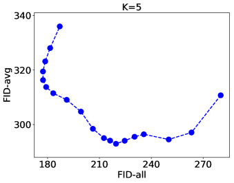
(a)

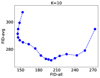
(b)

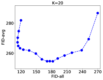
(c)

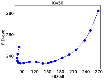
(d)

Figure 20: Ablation study on hyper-paramter K.

References

- Bińkowski et al. [2018] Bińkowski, M., Sutherland, D. J., Arbel, M., and Gretton, A. Demystifying mmd gans. In ICLR, 2018.
- Choi et al. [2020] Choi, Y., Uh, Y., Yoo, J., and Ha, J.-W. Stargan v2: Diverse image synthesis for multiple domains. In CVPR, 2020.
- Chrabaszcz et al. [2017] Chrabaszcz, P., Loshchilov, I., and Hutter, F. A downsampled variant of imagenet as an alternative to the cifar datasets. arXiv preprint arXiv:1707.08819, 2017.
- Deng et al. [2009] Deng, J., Dong, W., Socher, R., Li, L.-J., Li, K., and Fei-Fei, L. Imagenet: A large-scale hierarchical image database. In CVPR, pp. 248–255. Ieee, 2009.
- Dinh et al. [2016] Dinh, L., Sohl-Dickstein, J., and Bengio, S. Density estimation using real nvp. arXiv preprint arXiv:1605.08803, 2016.
- Goodfellow et al. [2014] Goodfellow, I. J., Pouget-Abadie, J., Mirza, M., Xu, B., Warde-Farley, D., Ozair, S., Courville, A., and Bengio, Y. Generative adversarial networks. arXiv preprint arXiv:1406.2661, 2014.
- Gulrajani et al. [2017] Gulrajani, I., Ahmed, F., Arjovsky, M., Dumoulin, V., and Courville, A. C. Improved training of wasserstein gans. NeurIPS, 30, 2017.
- Hardy et al. [2019] Hardy, C., Le Merrer, E., and Sericola, B. Md-gan: Multi-discriminator generative adversarial networks for distributed datasets. In IPDPS, pp. 866–877. IEEE, 2019.
- Heusel et al. [2017] Heusel, M., Ramsauer, H., Unterthiner, T., Nessler, B., and Hochreiter, S. Gans trained by a two time-scale update rule converge to a local nash equilibrium. NeurIPS, 30, 2017.
- Ho et al. [2020] Ho, J., Jain, A., and Abbeel, P. Denoising diffusion probabilistic models. NeurIPS, 33:6840–6851, 2020.
- Karras et al. [2019] Karras, T., Laine, S., and Aila, T. A style-based generator architecture for generative adversarial networks. In CVPR, pp. 4401–4410, 2019.
- Karras et al. [2020] Karras, T., Aittala, M., Hellsten, J., Laine, S., Lehtinen, J., and Aila, T. Training generative adversarial networks with limited data. In Proc. NeurIPS, 2020.
- Kingma & Welling [2013] Kingma, D. P. and Welling, M. Auto-encoding variational bayes. arXiv preprint arXiv:1312.6114, 2013.
- Krizhevsky et al. [2009] Krizhevsky, A., Hinton, G., et al. Learning multiple layers of features from tiny images. 2009.
- Kynkäänniemi et al. [2019] Kynkäänniemi, T., Karras, T., Laine, S., Lehtinen, J., and Aila, T. Improved precision and recall metric for assessing generative models. NeurIPS, 32, 2019.
- McMahan et al. [2017] McMahan, B., Moore, E., Ramage, D., Hampson, S., and y Arcas, B. A. Communication-efficient learning of deep networks from decentralized data. In Artificial intelligence and statistics, pp. 1273–1282. PMLR, 2017.
- Naeem et al. [2020] Naeem, M. F., Oh, S. J., Uh, Y., Choi, Y., and Yoo, J. Reliable fidelity and diversity metrics for generative models. In ICML, pp. 7176–7185. PMLR, 2020.
- Puccetti et al. [2020] Puccetti, G., Rüschendorf, L., and Vanduffel, S. On the computation of wasserstein barycenters. Journal of Multivariate Analysis, 176:104581, 2020.
- Ramesh et al. [2022] Ramesh, A., Dhariwal, P., Nichol, A., Chu, C., and Chen, M. Hierarchical text-conditional image generation with clip latents. arXiv preprint arXiv:2204.06125, 2022.
- Rasouli et al. [2020] Rasouli, M., Sun, T., and Rajagopal, R. Fedgan: Federated generative adversarial networks for distributed data. arXiv preprint arXiv:2006.07228, 2020.
- Rüschendorf & Uckelmann [2002] Rüschendorf, L. and Uckelmann, L. On the n-coupling problem. Journal of multivariate analysis, 81(2):242–258, 2002.
- Sajjadi et al. [2018] Sajjadi, M. S., Bachem, O., Lucic, M., Bousquet, O., and Gelly, S. Assessing generative models via precision and recall. NeurIPS, 31, 2018.
- Salimans et al. [2016] Salimans, T., Goodfellow, I., Zaremba, W., Cheung, V., Radford, A., and Chen, X. Improved techniques for training gans. NeurIPS, 29, 2016.
- Sohl-Dickstein et al. [2015] Sohl-Dickstein, J., Weiss, E., Maheswaranathan, N., and Ganguli, S. Deep unsupervised learning using nonequilibrium thermodynamics. In ICML, pp. 2256–2265. PMLR, 2015.
- Su et al. [2023] Su, X., Song, J., Meng, C., and Ermon, S. Dual diffusion implicit bridges for image-to-image translation. In ICLR, 2023.
- Theis et al. [2016] Theis, L., van den Oord, A., and Bethge, M. A note on the evaluation of generative models. In ICLR, pp. 1–10, 2016.
- Villani et al. [2009] Villani, C. et al. Optimal transport: old and new, volume 338. Springer, 2009.
- Wu et al. [2022] Wu, Y., Kang, Y., Luo, J., He, Y., Fan, L., Pan, R., and Yang, Q. Fedcg: Leverage conditional gan for protecting privacy and maintaining competitive performance in federated learning. In IJCAI, 2022.
- Yonetani et al. [2019] Yonetani, R., Takahashi, T., Hashimoto, A., and Ushiku, Y. Decentralized learning of generative adversarial networks from non-iid data. arXiv preprint arXiv:1905.09684, 2019.