Risk Bounds for Quantile Additive Trend Filtering

Abstract

This paper investigates risk bounds for quantile additive trend filtering, a method gaining increasing significance in the realms of additive trend filtering and quantile regression. We investigate the constrained version of quantile trend filtering within additive models, considering both fixed and growing input dimensions. In the fixed dimension case, we discover an error rate that mirrors the non-quantile minimax rate for additive trend filtering, featuring the main term $n^{-2r/(2r+1)}V^{2/(2r+1)}$, when the underlying quantile function is additive, with components whose $(r-1)$th derivatives are of bounded variation by $V$. In scenarios with a growing input dimension $d$, quantile additive trend filtering introduces a polynomial factor of $d^{(2r+2)/(2r+1)}$. This aligns with the non-quantile variant, featuring a linear factor $d$, particularly pronounced for larger $r$ values. Additionally, we propose a practical algorithm for implementing quantile trend filtering within additive models, using dimension-wise backfitting. We conduct experiments with evenly spaced data points or data that samples from a uniform distribution in the interval $[0,1]$, applying distinct component functions and introducing noise from normal and heavy-tailed distributions. Our findings confirm the estimator’s convergence as $n$ increases and its superiority, particularly in heavy-tailed distribution scenarios. These results deepen our understanding of additive trend filtering models in quantile settings, offering valuable insights for practical applications and future research.

Keywords Total Variation, nonparametric quantile regression, additive trend filtering.

1 Introduction

Quantile regression has been considered robust thus with its broad application in different fields (Coad et al., 2006; Sanderson et al., 2006; Perlich et al., 2007; Benoit and Van den Poel, 2009; Wasko and Sharma, 2014; Pata and Schindler, 2015; Belloni et al., 2023). The quantile trend filtering results in trend filtering estimator with smooth structures. It leans estimator by regularizing the total variation of $r$th discrete derivative of quantiles of signals. In the field of image processing, total variation smoothing penalties have gained significant attention (Rudin et al., 1992). These penalties enable edge detection and permit sharp breaks in gradients, surpassing the limitations of conventional Sobolev penalties. The quantile fused lasso is a special case of quantile trend filtering when $r=0$. The risk bound for quantile trend filtering has been studied by Madrid Padilla and Chatterjee (2022), which established the minimax rate for univariate trend filtering under the quantile loss with minor assumptions of the data generation mechanism.

Additive models, initially introduced by Friedman and Stuetzle (1981) provide a useful tool for dimension reduction and have been studied in various contexts, including Cox regression (Cox, 1972), logistic regression (Hastie and Tibshirani, 1987), and exponential family data distributions (Hastie, 2017). Additive models have been highly regarded for their pragmatic approach to nonparametric regression modeling, offering a way to mitigate the challenges posed by the curse of dimensionality (Breiman and Friedman, 1985; Hastie, 2017). In recent years, the focus of research on additive models has shifted towards high-dimensional nonparametric estimation, with an emphasis on inducing sparsity in the component functions, the seminal works are Lin and Zhang (2006); Ravikumar et al. (2009); Meier et al. (2009); Lou et al. (2016); Petersen et al. (2016). Notably, Sadhanala and Tibshirani (2017) derived fast error rates for additive trend filtering estimates, demonstrating their minimax optimality under sub-Gaussian errors.

The estimator of interest in this paper is the quantile additive trend filtering, offering a dual benefit of dimension reduction and robust regression. Consequently, we conducted an examination of risk bounds for quantile additive trend filtering.

Our contributions are: We investigated the risk bounds for a constrained version of quantile trend filtering in additive models. Quantile additive models are built around the univariate trend filtering estimator, defined by constraining according to the sum of $\ell_{1}$ norms of discrete derivatives of the component functions, and a quantile loss is applied. When the underlying quantile function is additive, with components whose $(r-1)$th derivatives are of bounded variation by $V$, we derived error rates for $(r-1)$th order quantile additive trend filtering. This rate is $n^{-2r/(2r+1)}V^{2/(2r+1)}\max\{1,V^{(2r-1)/(2r+1)}\}$ for a fixed input dimension $d$ (under weak assumptions). This rate contains the main term $n^{-2r/(2r+1)}V^{2/(2r+1)}$, which is the same as the non-quantile minimax rate in Sadhanala and Tibshirani (2017). It also includes an extra term, which is of order ${\mathcal{O}}(1)$ if $V={\mathcal{O}}(1)$. Such a value of $V$ is referred to as a canonical scaling, as described in Madrid Padilla and Chatterjee (2022); Sadhanala et al. (2016).

Additionally, we explored error rates for quantile trend filtering in additive models where the input dimension ($d$) increases with the sample size ($n$). Through this analysis, we demonstrated that it exhibits an error rate that includes a polynomial factor of $d^{(2r+2)/(2r+1)}$ multiplied by the fixed dimension error rate. In comparison, the non-quantile version, which has a linear factor of $d$, aligns with the nature of quantile additive trend filtering models for large values of $r$. Our rates, are minimax up to logarithmic factors, in fixed dimension case, and off by a small factor in the growing dimension setting, aligning closely with the minimax rates for mean estimation in additive trend filtering, as discussed in Sadhanala and Tibshirani (2017), which primarily considers sub-Gaussian errors. Our contribution takes a step beyond by introducing and justifying minor assumptions and proves that the constrained quantile trend filtering estimator is robust to heavy-tailed (with no moments existing) distributions of the errors.

Furthermore, we developed an algorithm for performing quantile trend filtering in additive models. This algorithm involves a backfitting approach for each dimension. We conducted simulations under multiple scenarios using evenly spaced data points between $[0,1]$ or data that samples from a uniform distribution of $[0,1]$. Each component function of a dimension was applied differently to the input data, and we introduced noise from either normal or heavy-tailed distributions. Our experiments demonstrate that the quantile additive trend filtering estimator converges as $n$ increases, as theory elaborated, and it revealed that it outperforms additive trend filtering models, especially for heavy-tailed distributions, and outperforms quantile smoothing splines in most cases.

2 Previous Work

2.1 Quantile Trend Filtering

In the analysis presented in Madrid Padilla and Chatterjee (2022), the constrained univariate quantile trend filtering estimator is given by

$$\min_{\theta\in{\mathcal{R}}^{n},TV^{(r)}(\theta)\leq V}\sum_{i=1}^{n}\rho_{\tau}(y_{i}-\theta_{i}),$$

where $\rho_{\tau}(x)=u\left\{\tau-I(u<0)\right\}=\max\left\{\tau x,(\tau-1)x\right\}$ is the check function. It involves the $r$th order total variation $TV^{(r)}(\theta)$ which is equal to the Riemann approximation to the integral $\int_{[0,1]}\left|f^{(r)}(t)\right|dt$, where $f$ is a $r$ times differentiable function on grid $(1/n,\dots,n/n)$. Hence, it is reasonable to consider $TV^{(r)}(\theta)$ as being of order ${\mathcal{O}}(1)$.

For both the constrained and penalized versions of univariate quantile trend filtering, Madrid Padilla and Chatterjee (2022) show that the risk bounds achieve the minimax rate, up to logarithmic factors. This holds true when the $(r-1)$th discrete derivative of the true vector of quantiles belongs to the class of bounded variation signals.

2.2 Additive Models and Additive Trend Filtering

The additive model has a format of

$$y_{i}=\mu+\sum_{j=1}^{d}f_{0j}(x_{ij})+\epsilon_{i}.$$ (1)

The $\mu$ is an overall mean parameter, and $f_{0j}$ is a univariate function. The errors $\epsilon_{i}$ are i.i.d. with mean zero. Furthermore, for identifiability, it is required that $\sum_{i=1}^{n}f_{0j}(x_{ij})=0$.

In Sadhanala and Tibshirani (2017), additive trend filtering was introduced as a regularization method in additive models to create smoother component functions. It involves regularizing each component function based on the total variation of its $r$th derivative (discrete) for a chosen integer $r\geq 1$. This regularization yields $(r-1)$th degree piecewise polynomial components. For instance, when $r=1$, it results in piecewise constant components, while $r=2$ leads to piecewise linear, and $r=3$ to piecewise quadratic, and so on. Trend filtering is favored for its favorable theoretical and computational properties, largely due to the localized nature of the total variation regularization it employs.

Falling factorial representation

The falling factorial representation serves as an alternative means to express additive trend filtering estimates in basis form. In this representation, each component is represented as a linear combination of basis functions, with coefficients subject to regularization.

The works of Tibshirani (2014), Wang et al. (2015), and Sadhanala and Tibshirani (2017) demonstrate that the univariate and additive trend filtering problem can be interpreted as a sparse basis regression problem using these functions. The falling factorial representation is employed to derive rapid error rates, highlighting its utility in trend filtering.

3 Quantile Trend Filtering For Additive Models

Before we define the estimator, let us introduce the necessary definitions and notation. We let $r\in N_{\geq 0}$, and we define $D^{(x,r)}\in\mathbb{R}^{(n-r)\times n}$ as a $r$-th order difference operator, for $r=1$, we define the first order operator as

$$D^{(x,1)}=\begin{bmatrix}-1&1&0\dots&0&0\\ 0&-1&1\dots&0&0\\ \dots\\ 0&0&0\dots&-1&1\end{bmatrix}\in\mathbb{R}^{(n-1)\times n},$$ (2)

$$D^{(x,1)}(\theta)=(\theta_{2}-\theta_{1},\dots,\theta_{n}-\theta_{n-1})^{\top}.$$ (3)

Recursively, we define operators for $r=2,3,\dots$, and these trend filtering operators are constructed based on $x$, forming a $\mathbb{R}^{(n-r)\times n}$ dimensional matrix:

$$D^{(x,r)}=D^{(x,1)}\text{diag}\left(\frac{r-1}{x_{r}-x_{1}},\dots,\frac{r-1}{x_{n}-x_{n-(r-1)}}\right)D^{(x,r-1)}.$$ (4)

Note that the matrix $D^{(x,1)}$ in (4) is the $(n-r)\times(n-(r-1))$ version of the difference operator in (2).

For example, for $r=2$, we have a $\mathbb{R}^{(n-1-1)\times n}$ dimensional matrix

$$D^{(x,1+1)}=D^{(x,1)}\text{diag}\left(\frac{1}{x_{2}-x_{1}},\dots,\frac{1}{x_{n}-x_{n-1}}\right)D^{(x,1)},$$ (5)

where the first $D^{(x,1)}$ is defined as

$$D^{(x,1)}=\begin{bmatrix}-1&1&0\dots&0&0\\ 0&-1&1\dots&0&0\\ \dots\\ 0&0&0\dots&-1&1\end{bmatrix}\in\mathbb{R}^{(n-1-1)\times(n-1)}.$$ (6)

Also note, for $r=0$, we have $D^{(x,0)}=I$, the identity operator and $D^{(x,0)}(\theta)=\theta$.

The constrained quantile additive trend filtering (CQATF) estimator $\hat{\theta}^{(r)}$ is derived from the problem (7):

$$\min_{\begin{subarray}{c}\theta\in K^{(x,r)}(V)\coloneqq\left\{\theta\in\mathbb{R}^{n},\theta=\sum_{j=1}^{d}\theta_{j},\right.\\ \left.\sum_{j=1}^{d}\left\lVert D^{(x_{j},r)}\theta_{j}\right\rVert_{1}\leq V,\sum_{i=1}^{n}\theta_{ij}=0\right\}\end{subarray}}\sum_{i=1}^{n}\rho_{\tau}(y_{i}-\sum_{j=1}^{d}\theta_{ij}).$$ (7)

This constrained quantile additive trend filtering estimator is distinct from the additive trend filtering version, represented as:

$$\min_{\begin{subarray}{c}\theta_{1},\dots,\theta_{d}\in\mathbb{R}^{n},\sum_{j=1}^{d}\left\lVert D^{(x_{j},r)}\theta_{j}\right\rVert_{1}\leq V\\ \text{s.t. }\quad 1^{\top}\theta_{j}=0,j=1,\dots,d\end{subarray}}\frac{1}{2}\left\lVert y-\sum_{j=1}^{d}\theta_{j}\right\rVert_{2}^{2}.$$ (8)

In the above two estimators, we define the vector $\theta_{j}=(\theta_{1j},\dots,\theta_{nj})\in\mathbb{R}^{n}$. And we let $n$ inputs $\left\{x_{1},\dots,x_{n}\right\}$ be i.i.d. random variables from ${\mathcal{X}}$, and each input data point is a vector $x_{i}=(x_{i1},\dots,x_{id})$. Furthermore, we sort the $j$th component of inputs into increasing order, i.e., $x_{j}=(x_{1j},x_{2j},\dots x_{nj})=(x_{(1)j},x_{(2)j},\dots,x_{(n)j}),j=1,\dots,d.$

The study by Tibshirani (2014) uncovered that the estimator for $r$-th order trend filtering is equivalent to penalized total variation of the $r$-th derivative of a function within a function space defined by the falling factorial basis. If we represent the assessments of the $j$-th component function $f_{j}$ in the manner of the relationship:

$$\theta_{ij}=f_{j}(x_{ij}),i=1,\dots,n,j=1,\dots,d.$$ (9)

The following problem is equivalent to the problem in Equation (7). The estimator $\hat{f}^{(r)}_{{\mathcal{H}}}$ is obtained by solving

$$\min_{\begin{subarray}{c}f\in{\mathcal{F}}^{(r)}(V)\coloneqq\left\{f=\sum_{j=1}^{d}f_{j}:f_{j}\in{\mathcal{H}}_{j},\right.\\ \left.\sum_{j=1}^{d}TV(f_{j}^{(r-1)})\leq V,\sum_{i=1}^{n}f_{j}(x_{ij})=0\right\}\end{subarray}}\sum_{i=1}^{n}\rho_{\tau}(y_{i}-\sum_{j=1}^{d}f_{j}(x_{ij})),$$ (10)

where ${\mathcal{F}}^{(r)}(V)$ is a function class such that for an element $f$ in the class, $f:[0,1]^{d}\rightarrow\mathbb{R}$. And the ${\mathcal{H}}_{j}$ is the span of the falling factorial basis over the $j$-th dimension, and $f_{j}^{(r-1)}$ is the $(r-1)$th weak derivative of $f_{j}$. Furthermore, the $TV$ operator is defined as below.

Definition 3.1.

For a function $f:[0,1]\rightarrow\mathbb{R}$, its total variation is defined as

$$TV(f)=\sup\left\{\sum_{i=1}^{p}\left|f(z_{i+1})-f(z_{i})\right|:\right.$$ (11)

$$\left.z_{1}<\dots z_{p}\text{ is a partition of }[0,1]\right\}.$$

And we define $TV^{(r)}$ as the total variation of the $(r-1)$th weak derivative of $f$. Thus, $TV^{(r)}(f)=TV(f^{(r-1)})$.

It is well known that the total variation of the $r-1$ derivative of $r$ differential function is $\int_{[0,1]}\left|f^{(r)}(t)\right|dt$, if considering the Riemann approximation of the integral.

An early work on quantile regression for additive models also employed the $TV$ operator as a regularization technique, as discussed in Koenker (2011). However, it’s worth noting that this work specifically focused on the case when $r=2$. Thus, our task is to provide the risk bounds for estimators in Equation (7) and (10).

Penalized quantile additive trend filtering

As demonstrated in Sadhanala and Tibshirani (2017) and Madrid Padilla and Chatterjee (2022), Equation (7) can be transformed into a penalized version by introducing a tuning parameter $\lambda$:

$$\min_{\begin{subarray}{c}\theta_{1},\dots,\theta_{d}\in\mathbb{R}^{n}\\ \text{s.t. }\sum_{i=1}^{n}1^{\top}\theta_{j}=0.\end{subarray}}\sum_{i=1}^{n}\rho_{\tau}(y_{i}-\sum_{j=1}^{d}\theta_{ij})+\lambda\sum_{j=1}^{d}\left\lVert D^{(x_{j},r)}\theta_{j}\right\rVert_{1}.$$ (12)

For the sake of practical implementation, we will employ the above estimator in our experiments.

4 Main Results

4.1 Notations

Given a distribution $Q$, and a set of i.i.d. points $x=\left\{x_{1},\dots,x_{n}\right\}\subseteq[0,1]^{d}$, $i=1,\dots,n$ from $Q$, we define the $L_{2}$, euclidean and empirical inner products $\Big{\langle}\cdot,\cdot\Big{\rangle}_{L_{2}}$ $\Big{\langle}\cdot,\cdot\Big{\rangle}_{2}$ $\Big{\langle}\cdot,\cdot\Big{\rangle}_{n}$ as below.

Let ${\mathcal{X}}$ be $[0,1]^{d}$, for two functions $f:{\mathcal{X}}\rightarrow\mathbb{R}$ and $g:{\mathcal{X}}\rightarrow\mathbb{R}$, we define

$$\Big{\langle}f,g\Big{\rangle}_{L_{2}}=\int_{{\mathcal{X}}}f(x)g(x)dQ(x),$$ (13)

$$\Big{\langle}f,g\Big{\rangle}_{2}=\sum_{i=1}^{n}f(x_{i})g(x_{i}),$$ (14)

$$\Big{\langle}f,g\Big{\rangle}_{n}=\frac{1}{n}\sum_{i=1}^{n}f(x_{i})g(x_{i}).$$ (15)

Hence, we define the $L_{2}$ norm $\left\lVert\cdot\right\rVert_{L_{2}}$ as $\left\lVert f\right\rVert_{L_{2}}^{2}=\Big{\langle}f,f\Big{\rangle}_{L_{2}}=\int_{{\mathcal{X}}}f(x)^{2}dQ(x)$. We have empirical norm $\left\lVert\cdot\right\rVert_{n}$ as $\left\lVert f\right\rVert_{n}=\Big{\langle}f,f\Big{\rangle}_{n}=\frac{1}{n}\sum_{i=1}^{n}f(x_{i})^{2}$. The $\left\lVert\cdot\right\rVert_{2}$ and $\left\lVert\cdot\right\rVert_{\infty}$ are defined as $\left\lVert f\right\rVert_{2}^{2}=n\left\lVert\cdot\right\rVert_{n}^{2}$, and $\left\lVert f\right\rVert_{\infty}=\max_{i=1,\dots n}\left|f(x_{i})\right|$. We also use the $\left\lVert\cdot\right\rVert$ as the common euclidean norm.

For a functional $\nu$, we let $B_{\nu}(\epsilon)$ for the $\nu$-ball of radius $\epsilon>0$, i.e., $B_{\nu}(\epsilon)=\left\{f:\nu(f)\leq\epsilon\right\}$. So $B_{n}(\epsilon)$ for the $\left\lVert\cdot\right\rVert_{n}$-ball of radius $\epsilon$, and $B_{L_{2}}(\epsilon)$ for the $\left\lVert\cdot\right\rVert_{L_{2}}$-ball of radius $\epsilon$, and $B_{\infty}(\epsilon)$ for the $\left\lVert\cdot\right\rVert_{\infty}$-ball of radius $\epsilon$.

For an additive function $f=\sum_{j=1}^{d}f_{j}$, its input is a vector $x_{i}=(x_{i1},\dots,x_{id})$, and we have

$$f(x_{i})=\sum_{j=1}^{d}f_{j}(x_{ij}).$$ (16)

In this paper, we reserve index $i$ for data point, and $j$ for the component, and for any function $f$, we use $f_{i}$ as a shorthand for $f(x_{i})$, and $f_{ij}$ for $f_{j}(x_{ij})$.

Assumption 4.1.

Assume the inputs are sorted in each dimension such that

$$0<x_{1j}<x_{2j}\dots<x_{nj}\leq 1,\quad j=1,\dots,d.$$ (17)

Assumption 4.1 is minor as we can always scale the inputs. The same constraint is used in the analysis in Sadhanala and Tibshirani (2017).

For $(r-1)$th order polynomial, its $(r-1)$th order derivatives are a constant, and its $r$th order derivatives are zero. The null space of $TV^{(r)}$ is the $(r-1)$th order polynomial. For the sake of clarity in our writing, we will use $J$ to represent $TV^{(r)}$.

It is well known that the operator $J$ is a seminorm and its domain is contained in the space of $(r-1)$th times weakly differentiable functions. Furthermore, its null space contains all $(r-1)$th order polynomials, i.e., $J(g)=0$ for all $g(x)=x^{l},l=0,\dots,r-1$.

Let $\left\{x_{1},\dots,x_{n}\right\}$ satisfied the Assumption 4.1. Conditioned on $x_{i}$, then a $\tau$-quantile of $y_{i}$ is given as

$$f^{*}(x_{i})=\arg\min_{a\in\mathbb{R}}\operatorname*{{\mathbb{E}}}\left[\rho_{\tau}(y_{i}-a)|x_{i}\right],$$ (18)

where the expectation is taken with respect to $y_{i}$ conditioned on $x_{i}$.

Assumption 4.2.

For $f^{*}$ as in (18), we assume that

$$\sum_{i=1}^{n}f_{j}^{*}(x_{ij})=0,\quad\text{for }j=1\dots d.$$ (19)

Our Assumption 4.2 is consistent to the Assumption B1 by Sadhanala and Tibshirani (2017).

Assumption 4.3.

There exists a constants $L>0$ and $\underline{\hbox{\set@color$f$}}>0$ such that for any positive integer $n$ and any function $\delta$ with $\left\lVert\delta\right\rVert_{\infty}\leq L$ we have that

$$\left|F_{y_{i}|x_{i}}(f_{i}^{*}+\delta_{i})-F_{y_{i}|x_{i}}(f_{i}^{*})\right|\geq\underline{\hbox{\set@color$f$}}\left|\delta_{i}\right|,$$ (20)

where $F_{y_{i}|x_{i}}$ is the conditional CDF of $y_{i}$.

Similar conditions are assumed by Assumption A of Madrid Padilla and Chatterjee (2022) and Assumption 4 of Shen et al. (2022). Assumption 4.3 ensures that the conditional quantile of $y_{i}$ given $x_{i}$ is uniquely defined and there is a uniformly linear growth of the CDF around a neighborhood of the quantile.

4.2 Results for CQATF Estimator

Using an abuse of notation, let $\delta$ be the evaluation of a function $\delta$ at $x_{1},\dots,x_{n}$. Our loss function is given by the function $\Delta_{n}^{2}(\delta):\mathbb{R}^{n}\rightarrow\mathbb{R}$ defined as

$$\Delta_{n}^{2}(\delta)=\frac{1}{n}\sum_{i=1}^{n}\min\left\{\left|\delta(x_{i})\right|,\delta(x_{i})^{2}\right\},$$ (21)

which, up to constants, is a Huber loss, see Huber (1992). The main reason why our bounds are for the Huber loss is that this loss naturally appears as a lower bound to the quantile population loss.

Theorem 4.4.

Let $\left\{y_{i}\right\}_{i=1}^{n}$ be any sequence of independent random variables which satisfies Assumption 4.3 and be the sequence of $\tau$ quantiles of $y_{i}$. Suppose Assumption 4.1 holds on the data inputs, and Assumption 4.2 holds on $f^{*}$. Assume $f^{*}=\sum_{j=1}^{d}f_{j}^{*}$, where $f^{*}\in{\mathcal{F}}^{(r)}(V)$ and $\sum_{j=1}^{d}J(f_{j}^{*})=V^{*}$, if $V$ is chosen such that $V\geq V^{*}=\sum_{j=1}^{d}J(f_{j}^{*})$, then

$$\Delta_{n}^{2}(\hat{f}_{{\mathcal{H}}}^{(r)}-f^{*})=$$ (22)

$$O_{pr}\left[n^{-2r/(2r+1)}V^{2/(2r+1)}\max\left\{1,V^{(2r-1)/(2r+1)}\right\}\right].$$

Remark 4.5.

Theorem 4.4 extends Theorem 1 in Sadhanala and Tibshirani (2017) to quantile regression, differing from their Theorem 1 by the inclusion of an additional factor:

$$\max\left\{1,V^{(2r-1)/(2r+1)}\right\},$$

which can go to infinity if $V$ grows to infinity. However, under the canonical scaling $V^{*}={\mathcal{O}}(1)$ as mentioned in Madrid Padilla and Chatterjee (2022); Sadhanala et al. (2016), one can choose $V={\mathcal{O}}(1)$ as well and thus the above term is also ${\mathcal{O}}(1)$. The rate is minimax up to log factors in that sense that it matches the minimax rates of mean estimation for additive trend filtering, see Sadhanala and Tibshirani (2017).

4.3 Error bounds for a growing dimension $d$

In this subsection, we allow the input dimension $d$ to grow with the sample size $n$. Furthermore, to produce an error rate linearly dependent on the growing dimension $d$, we add the below assumption, which is also assumed as the Assumption A3 in Sadhanala and Tibshirani (2017).

Assumption 4.6.

The input points $x_{i},i=1\dots n$ satisfying Assumption 4.1 are i.i.d. from a continuous distribution $F$ supported on $[0,1]^{d}$, that decomposes as $F=F_{1}\times\cdots\times F_{d}$, where the density of each $F_{j}$ is lower and upper bounded by constants $b_{1};b_{2}>0,\text{ for }j=1,\dots,d$.

Assumption 4.7.

We define the maximum width across any two data points as

$$w=\max_{\begin{subarray}{c}i=1,\dots,n-1\\ j=1,\dots,d\end{subarray}}\left|x_{ij}-x_{(i-1)j}\right|,$$ (23)

then we assume that $w\lesssim\frac{\log n}{n}$.

Remark 4.8.

Assumption 4.7 would be satisfied with probability approaching 1 by Lemma 5 in Wang et al. (2015), for $x_{1j},\dots,x_{nj}$ that are i.i.d. from a uniform distribution $[0,1]$.

Theorem 4.9.

Let $\left\{y_{i}\right\}_{i=1}^{n}$ be any sequence of independent random variables which satisfies Assumption 4.3 and be the sequence of $\tau$ quantiles of $y_{i}$. Let $\left\{x_{i}\right\}_{i=1}^{n}$ be the input points which satisfy Assumption 4.1 and 4.6. And suppose Assumption 4.2 holds on $f^{*}$. Assume $f^{*}=\sum_{j=1}^{d}f_{j}^{*}$, where $f^{*}\in{\mathcal{F}}^{(r)}(V)$ and $\sum_{j=1}^{d}J(f_{j}^{*})=V^{*}$, if $V$ is chosen such that $V\geq V^{*}=\sum_{j=1}^{d}J(f_{j}^{*})$, then

$$\Delta_{n}^{2}(\hat{f}_{{\mathcal{H}}}^{(r)}-f^{*})=O_{pr}\left[d^{(2r+2)/(2r+1)}n^{-2r/(2r+1)}V^{2/(2r+1)}\right.$$ (24)

$$\left.\max\left\{1,V^{(2r-1)/(2r+1)}\right\}\right].$$

Remark 4.10.

Theorem 4.9 generalizes Theorem 2 in Sadhanala and Tibshirani (2017) to the quantile regression setting, with a difference that our upper bound contains an extra term. This is the factor

$$\max\left\{1,V^{(2r-1)/(2r+1)}\right\},$$

which can go to infinity if $V$ grows to infinity. However, under the canonical scaling $V^{*}={\mathcal{O}}(1)$ one can choose $V={\mathcal{O}}(1)$ as well and thus the above term is also ${\mathcal{O}}(1)$. The factor $d^{(2r+2)/(2r+1)}$ compared to Theorem 2 in Sadhanala and Tibshirani (2017) is $d$, and for large $r$, these two terms tend to be the same, making our rate essentially minimax up to log factors.

5 Experiments

We sampled $n\in\{100,500,1000\}$ input points in $d=10$ dimensions, by assigning the inputs along each dimension $x_{j}=(x_{1j}\dots x_{nj})$. As benchmark methods, we consider the usual (mean regression) penalized additive trend filtering estimator of order $r=2$ and $r=3$ denoted as ATF1 and ATF2 respectively, quantile smoothing splines (QS) (introduced in Koenker et al. (1994)) which we implement using the R package “fields”. Notice that ATF1 and ATF2 only provide estimates for $\tau=0.5$. As for quantile trend filtering, we consider the penalized estimator (LABEL:70) with orders $r=2$ and $r=3$ which we denote as QATF1 and QATF2 respectively. These are implemented using a block coordinate descent (BCD) algorithm, which uses a subroutine based on ADMM algorithm in R. We employ the R package “glmgen”, where ADMM is implemented, similar to the approach in Brantley et al. (2020).

The algorithm we used for quantile additive trend filtering is the backfitting approach that is described in Algorithm 1. In words, the algorithm cycles over $j=1\dots d$, and at each step updates the estimate for component $j$ by applying univariate quantile trend filtering to the $j$th partial residual (i.e., the current residual excluding component j). The non-quantile additive trend filtering is implemented by replacing the step (ii) in Algorithm 1 with the least squared loss. This resembles the algorithm used in Sadhanala and Tibshirani (2017), who shows that their approach is equivalent to the block coordinate descent applied to the dual, and the optimum can be obtained at convergence.

Algorithm 1 is equivalent to exact blockwise minimization, applied to problem (LABEL:70) over the coordinate blocks $j$, $j=1\dots d$. A general treatment of BCD is given in Tseng (2001), who shows that for a convex criterion that decomposes into smooth plus separable terms, as does that in (LABEL:70), all limit points of the sequence of iterates produced by BCD are optimal solutions. Thus, our algorithm for quantile additive trend filtering will produce the optimum solutions.

1:   Given responses $y_{i}\in\mathbb{R}$ and input points $x_{i}\in\mathbb{R}^{d}$, $i=1\dots n$.

2:  Set $t=0$ and initialize $\theta_{j}^{(0)}=0$, for $j=1,\dots d$.

3:  for $t=1,2,3,\dots$ (unitl converge) do

4:     for $j=1,2,\cdots,d$ do

5:        (i) Set response $r_{i}$, $r_{i}=y_{i}-\sum_{l<j}\theta_{il}^{(t)}-\sum_{l>j}\theta_{il}^{(t-1)}$, for $i=1,\dots,n$.

6:        (ii) $\theta_{j}^{(t)}=\operatorname*{arg\,min}_{\theta_{j}}\sum_{i=1}^{n}\rho_{\tau}(r_{i}-\theta_{ij})+\lambda\left\lVert D^{(x_{j},r)}\theta_{j}\right\rVert_{1},\text{s.t.}\sum_{i=1}^{n}1^{\top}\theta_{j}=0.$

7:     end for

8:  end for

9:  Return $\hat{\theta}_{j}$, $j=1,\dots,d$ (parameters $\theta_{j}^{t}$ at convergence).

Algorithm 1 Backfitting for quantile additive trend filtering

For the different trend filtering based methods we consider values of $\lambda$ such that $\log_{10}(\lambda)$ is in a grid of 50 evenly spaced points between -7 and 5. For quantile splines, which empirically preferred smaller lambda values, we considered the grid from -14 to 1. We choose the $\lambda$ to be the value that minimizes the estimator $\hat{f}$’s mean squared error, $\frac{1}{n}\sum_{i=1}^{n}(\hat{f}-f^{*})^{2}$, with $f^{*}$ representing the true vector of quantiles.

(a) Scenario 1, $n=500$

(b) Scenario 1, $n=500$

(c) Scenario 2, $n=500$

(d) Scenario 2, $n=500$

(e) Scenario 3, $n=500$

(f) Scenario 3, $n=500$

(g) Scenario 4, $n=500$

(h) Scenario 4, $n=500$

(i) Scenario 5, $n=500$

(j) Scenario 5, $n=500$

(k) Scenario 6, $n=500$

(l) Scenario 6, $n=500$

Figure 1: Panels 1(a), 1(g), and 1(i), show $f^{*}$, the true median, for Scenarios 1, 4, and 5, respectively. Panels 1(c) and 1(e) show an instance of $f^{*}$, since each $x_{j}$ is itself randomly generated. Panel 1(k) shows the true qunatile curve for Scenario 6 associated with $\tau=0.9$. Panels 1(b), 1(d), 1(f), 1(h), 1(j), and 1(j), then show an instance of the true data for each scenario.

We then report the average mean squared error over 50 Monte Carlo replicates of the different competing methods. In each scenario, the data are generated as

$$y_{i}=\sum_{j=1}^{d}f_{j}^{*}(x_{ij})+\epsilon_{i},\quad,i=1,\dots,n$$ (25)

where $f_{j}^{*}$ is our component function where we provide its expression below. For the componentwise trends, we added different signals to different components. Here we provided its details:

We examined sinusoids with Doppler-like spatially varying frequencies:

$$g_{j}(x)=\sin\left(\frac{2\pi}{(x+0.1)^{j/10}}\right),\quad j=1,\dots,10.$$ (26)

We also examined piecewise linear frequencies:

$$h_{j}(x)=(x+0.1)*j,\quad j=1,\dots,10.$$ (27)

We then defined the component functions as $f_{j}^{*}=a_{j}g_{j}-b_{j}$, or $f_{j}^{*}=a_{j}h_{j}-b_{j}$, for $j=1\dots d$, where $a_{j}$, $b_{j}$ were chosen so that $f_{j}^{*}$ had empirical mean zero and empirical norm $\left\lVert f_{j}^{*}\right\rVert_{n}=1$, for $j=1,\dots,d$.

The errors $\left\{\epsilon_{i}\right\}_{i=1}^{n}$ are independent with $\epsilon_{i}\sim F_{i}$ for some distributions $F_{i}$ with $i\in[n]$. We examine different choices of our inputs and $F_{i}$’s that we consider.

In Scenarios 1, 4, 5, and 6, we consider equally spaced points $(1/n,2/n,\dots,1)$ for $x_{ij}$, where $j$ ranges from 1 to $d$. In the remaining Scenarios 2 and 3, we sample $x_{j}$ from a $d$-dimensional uniform distribution within the interval $[0,1]^{d}$. Additionally, in some of these scenarios, we introduce a transformation function $k:[0,1]\rightarrow\mathbb{R}$, which maps $x_{ij}$ differently for varying indices $i$. The transformed values serve as inputs for $f_{j}^{*}$. Our results are in Table 1. In addition, Figure 1 illustrates the true signals and one data set example for each of the different scenarios that we consider. Finally, we use Figure 2 to compare some fits among QATF, QS, and ATF.

Scenario 1 (Normal Errors). As component functions $f_{j}^{*}$ we consider the Doppler-like spatially varying frequencies ($g_{j}$ in (26)). We take the $F_{i}$’s to be $N(0,1)$. With normal errors and varying smoothness, this scenario lends itself perfectly to ATF. In Table 1, ATF1 is the best, with ATF2 extremely close. QATF1 and QATF2 both outperform QS, which is expected, given splines’ inability to adapt to heterogeneous smoothness. Figure 2(a) provides a demonstration of this distinction.

Scenario 2 (Cauchy Errors). We maintain the same component functions $f_{j}^{*}$ as in Scenario 1, while substituting the normal $N(0,1)$ with $\text{Cauchy}(0,1)$ errors. In this situation the errors have no mean. As a result, ATF1 and ATF2 completely breakdown as shown in Table 1 and Figure 2(b). In contrast, as expected, the quantile methods are robust and can still provide strong estimates, with QATF1 and QATF2 slightly outperforming QS, just as in Scenario 1.

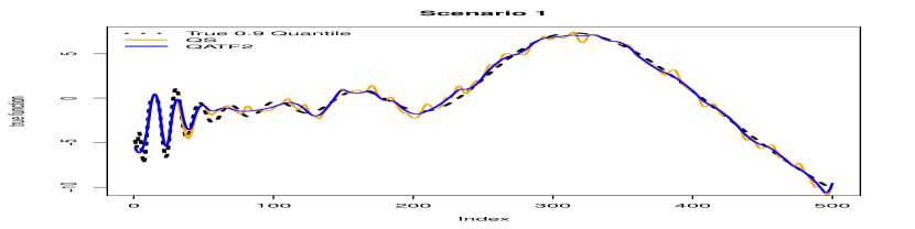
(a) Scenario 1, $n=500$

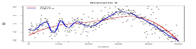
(b) Scenario 2, $n=500$

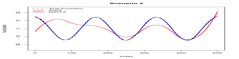
(c) Scenario 5, $n=500$

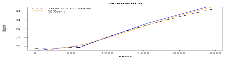
(d) Scenario 6, $n=2500$

Figure 2: Figure 2(a) plots QATF + QS on the true function $f^{*}$. Figure 2(b) plots QATF + ATF on real data. Figure 2(c) plots QATF + ATF on the true function $f^{*}$, and 2(d) plots QATF1 + QS on the true $0.9$ quantile.

Table 1: Average mean squared error, $\frac{1}{n}\sum_{i=1}^{n}(f_{i}^{*}-\hat{f}_{i})^{2}$, averaging over 50 Monte carlo simulations for the different methods considered. Captions are described in the text.

n	Scenario	tau	QATF1	QATF2	QS	ATF1	ATF2
500	1	0.5	0.196 ± 0.016	0.203 ± 0.016	0.274 ± 0.018	0.133 ± 0.007	0.138 ± 0.008
1000	1	0.5	0.113 ± 0.004	0.121 ± 0.004	0.168 ± 0.01	0.076 ± 0.003	0.083 ± 0.003
2500	1	0.5	0.057 ± 0.003	0.063 ± 0.003	0.1 ± 0.01	0.04 ± 0.002	0.042 ± 0.002
500	2	0.5	0.447 ± 0.035	0.47 ± 0.036	0.524 ± 0.034	24.348 ± 13.853	34.225 ± 30.885
1000	2	0.5	0.24 ± 0.021	0.259 ± 0.028	0.314 ± 0.021	88.983 ± 103.106	131.328 ± 146.261
2500	2	0.5	0.106 ± 0.005	0.114 ± 0.005	0.152 ± 0.009	46.117 ± 21.263	59.133 ± 27.468
500	3	0.5	0.191 ± 0.012	0.211 ± 0.013	0.254 ± 0.016	0.476 ± 0.076	0.447 ± 0.058
1000	3	0.5	0.102 ± 0.003	0.114 ± 0.004	0.156 ± 0.009	0.334 ± 0.051	0.319 ± 0.045
2500	3	0.5	0.041 ± 0.001	0.045 ± 0.001	0.085 ± 0.014	0.181 ± 0.029	0.173 ± 0.029
500	4	0.5	0.019 ± 0.005	0.056 ± 0.006	0.067 ± 0.008	0.025 ± 0.003	0.069 ± 0.007
1000	4	0.5	0.009 ± 0.002	0.028 ± 0.002	0.036 ± 0.003	0.014 ± 0.003	0.042 ± 0.002
2500	4	0.5	0.004 ± 0.001	0.015 ± 0.001	0.019 ± 0.001	0.007 ± 0.002	0.025 ± 0.002
500	5	0.5	0.198 ± 0.015	0.114 ± 0.014	0.118 ± 0.014	5851.976 ± 11575.592	9594.002 ± 19451.649
1000	5	0.5	0.106 ± 0.009	0.062 ± 0.007	0.06 ± 0.006	93.907 ± 104.356	111.286 ± 145.048
2500	5	0.5	0.05 ± 0.002	0.027 ± 0.001	0.028 ± 0.002	90.978 ± 35.759	116.3 ± 72.313
500	6	0.9	0.061 ± 0.023	0.094 ± 0.035	0.058 ± 0.021	NA	NA
1000	6	0.9	0.038 ± 0.011	0.056 ± 0.016	0.037 ± 0.01	NA	NA
2500	6	0.9	0.019 ± 0.005	0.031 ± 0.014	0.019 ± 0.005	NA	NA
500	6	0.1	0.077 ± 0.033	0.124 ± 0.041	0.069 ± 0.026	NA	NA
1000	6	0.1	0.037 ± 0.007	0.049 ± 0.012	0.037 ± 0.007	NA	NA
2500	6	0.1	0.019 ± 0.003	0.028 ± 0.005	0.018 ± 0.003	NA	NA

Scenario 3 (Heteroscedastic $t$ Errors). Once again, we take $f_{j}^{*}$ as in Scenarios 1 and 2. With regards to the $F_{i}$’s, we set $\epsilon_{i}=i^{1/2}/n^{1/2}v_{i}$, where the $v_{i}$’s are independent draws from $t(2)$. Here $t(2)$ denotes the t-distribution with 2 degrees of freedom. The empirical performances here are similar in nature to that of Scenario 2, but less extreme. ATF1 and ATF2 don’t completely fall apart, but QATF1, QATF2, and QS are all better fits.

Scenario 4 (Piecewise Linear Quantiles, $t$ Errors). We introduce a transform function $k(x_{ij})$ defined as follows:

$$k(x_{ij})=\begin{dcases}3x_{ij},&\text{for }i\in\left\{1\dots\left\lfloor{n/2}\right\rfloor\right\},\\ 3(1-x_{ij}),&\text{for }i\in\left\{{\left\lfloor{n/2}\right\rfloor}+1\dots n\right\}.\end{dcases}$$

The errors are then independent draws from $t(3)$. In terms of component functions, we consider piecewise linear frequencies ($h_{j}$ in (27)). Given that the true median curve exhibits a piecewise linear pattern, and the errors are heavy-tailed, Scenario 4 appears to be best suited for QATF1. This intuition is indeed confirmed in Table 1.

Scenario 5 (Sinusoidal Quantiles, Cauchy Errors). The signal is defined as $k(x_{ij})=\cos(6\pi x_{ij})$ for $i\in\left\{1\dots n\right\}$, and the error terms $\epsilon_{i}$ are generated from $\text{Cauchy}(0,1)$. In this scenario, the true median curve is infinitely differentiable. For the component functions $f_{j}^{*}$, we consider piecewise linear frequencies ($h_{j}$ in (27)). As in Scenario 2, Table 1 and Figure 2(c) illustrate the shortcomings of ATF when dealing with Cauchy errors, when compared to the QATF. Further, this scenario, with homogenous smoothness suits splines well, but Table 1 records QATF2 as a very close competitor.

Scenario 6 (Piecewise smooth quantiles, Heteroscedastic Errors).

We generate data $y$ as

$$y_{i}=\begin{cases}\left(\frac{0.25\sqrt{(i/n)}+1.375}{3}\right)v_{i}\quad i\in\left\{1,\dots,{\left\lfloor{n/2}\right\rfloor}\right\}\\ \left(\frac{7\sqrt{i/n}-2}{3}\right)v_{i}\quad i\in\left\{{\left\lfloor{n/2}\right\rfloor}+1,\dots,n\right\},\end{cases}$$

where the $v_{i}$ are independent draws from $t(2)$. Unlike the previous scenarios, Scenario 6 presents a case where the median is constant but the other quantiles change. By the nature of Scenario 6, one would expect QATF1 to be the best method as the pieces of the $0.9$th quantile curves can be well approximated by linear functions. Figure 2(d) demonstrates the effectiveness of QATF1 at capturing the changing quantiles, even with a constant median.

Overall, we see that the QATF estimator performs well across different scenarios and under the presence of heavy-tailed errors thereby supporting our theoretical findings.

6 Discussion

To summarize, in this paper we have studied quantile additive trend filtering. Our risk bounds generalize previous findings to the quantile setting. The main advantage of our results is that they hold under highly general conditions without requiring moment conditions and allowing for heavy-tailed distributions. It would be interesting to extend these tools to analyze all the other quantile additive models.

Appendix A Proofs

To complete our proofs for the theorems, we provide additional definitions.

Definition A.1.

The $r$-th order $TV$-ball of radius $V$ is defined as:

$$B_{J}(V)\coloneqq B_{TV}^{(r)}(V)=\left\{f:TV^{(r)}(f)=J(f)\leq V\right\}.$$ (28)

Definition A.2.

The $r$-th order trend filtering operator norm ball of radius $V$ as

$$BV^{(r)}(V)=\left\{\theta\in\mathbb{R}^{n}:\left\lVert D^{(x,r)}(\theta)\right\rVert_{1}\leq V\right\}.$$ (29)

Let $y\in\mathbb{R}^{n}$ be a vector of independent random variables and for a given quantile level $\tau\in(0,1)$. We define the Rademacher width and complexity as

Definition A.3.

For the function class ${\mathcal{F}}^{(r)}(V)$ defined in (10), we define its Rademacher width as

$$RW({\mathcal{F}}^{(r)}(V))=\operatorname*{{\mathbb{E}}}\left[\sup_{f\in{\mathcal{F}}^{(r)}(V)}\sum_{i=1}^{n}\xi_{i}f_{i}(x_{i})\mid\left\{x_{i}\right\}_{i=1}^{n}\right].$$ (30)

Definition A.4.

For the function class ${\mathcal{F}}^{(r)}(V)$ defined in (10), we define its Rademacher complexity

$$R({\mathcal{F}}^{(r)}(V))=\operatorname*{{\mathbb{E}}}\left[\sup_{f\in{\mathcal{F}}^{(r)}(V)}\frac{1}{n}\sum_{i=1}^{n}\xi_{i}f(x_{i})\right].$$ (31)

And we define its Empirical Rademacher complexity $R_{n}({\mathcal{F}}^{(r)}(V))=\frac{1}{n}RW({\mathcal{F}}^{(r)}(V))$.

We then define the empirical loss function as

$$\hat{M}(f)=\sum_{i=1}^{n}\hat{M}_{i}(f),$$ (32)

where each $\hat{M}_{i}(f)$ is defined as

$$\hat{M}_{i}(f)=\rho_{\tau}(y_{i}-f(x_{i}))-\rho_{\tau}(y_{i}-f^{*}(x_{i})).$$ (33)

We also define the population loss function as

$$M(f)\coloneqq\sum_{i=1}^{n}M_{i}(f),$$ (34)

where

$$M_{i}(f)\coloneqq\operatorname*{{\mathbb{E}}}\left[\rho_{\tau}(y_{i}-f(x_{i}))-\rho_{\tau}(y_{i}-f^{*}(x_{i}))|x_{i}\right].$$ (35)

Note, from (18), we know $f^{*}\in\operatorname*{arg\,min}M(f)$, and $M(f^{*})=0$.

Definition A.5.

The constrained quantile additive estimator defined in (10) will be

$$\hat{f}=\operatorname*{arg\,min}_{f\in{\mathcal{F}}^{(r)}(V)}\hat{M}(f),$$ (36)

By Definitions in (18) and (32), we have

$$\hat{M}(\hat{f})-\hat{M}(f^{*})\leq 0$$ (37)

as the basic inequality.

Lemma A.6.

For any $f,f^{*}\in{\mathcal{F}}^{(r)}(V)$, denote $\delta(x_{i})=f(x_{i})-f^{*}(x_{i})$, then we have

$$M_{i}(f)-M_{i}(f^{*}) =\int_{0}^{\delta(x_{i})}\left\{F_{y_{i}|x_{i}}(f^{*}(x_{i})+z)-F_{y_{i}|x_{i}}(f^{*}(x_{i}))\right\}dz.$$ (38)

Proof.

Let $I$ be the indicator function. By equation (B.3) in Belloni and Chernozhukov (2011),we have

$$\rho_{\tau}(w-v)-\rho_{\tau}(w)=-v(\tau-I(w\leq 0))+\int_{0}^{v}\left\{I(w\leq z)-I(w\leq 0)\right\}dz.$$ (39)

Given any $f$ and $x_{i}$, let $w=y-f^{*}(x_{i})$, $v=f(x_{i})-f^{*}(x_{i})$. Then taking conditional expectations on above equation with respect to $y_{i}$ conditioned on $x_{i}$ on both sides, we have

$$M_{i}(f)-M_{i}(f^{*}) =\operatorname*{{\mathbb{E}}}\left[\rho_{\tau}(y_{i}-f(x_{i}))-\rho_{\tau}(y_{i}-f^{*}(x_{i}))|x_{i}\right]$$ (40)

$$=\operatorname*{{\mathbb{E}}}\left[-\delta(x_{i})(\tau-I(y_{i}-f(x_{i})\leq 0))|x_{i}\right]$$

$$+\operatorname*{{\mathbb{E}}}\left[\int_{0}^{\delta(x_{i})}\left\{I(y_{i}-f^{*}(x_{i})\leq z)-I(y_{i}-f^{*}(x_{i}))\leq 0\right\}dz|x_{i}\right]$$

$$=0+\int_{0}^{\delta(x_{i})}\left\{F_{y_{i}|x_{i}}(f^{*}(x_{i})+z)-F_{y_{i}|x_{i}}(f^{*}(x_{i}))\right\}dz$$

$$=\int_{0}^{\delta(x_{i})}\left\{F_{y_{i}|x_{i}}(f^{*}(x_{i})+z)-F_{y_{i}|x_{i}}(f^{*}(x_{i}))\right\}dz,$$

for all $i=1,\dots,n$. ∎

Lemma A.7.

Assume Assumption 4.3 holds, then there exists $c_{0}$ such that for all $\delta=f-f^{*}$, we have

$$M(f^{*}+\delta)\geq c\Delta^{2}(\delta),$$

Proof.

Supposing that $\left|\delta(x_{i})\right|\leq L$, by Assumption 4.3 and Lemma A.6, we have

$$M_{i}(f)-M_{i}(f^{*}) \geq\int_{0}^{\delta(x_{i})}\underline{\hbox{\set@color$f$}}\left|z\right|dz$$ (41)

$$=\frac{\underline{\hbox{\set@color$f$}}\delta(x_{i})^{2}}{2}$$

Supposing that $\delta_{i}>L$, by Lemma A.6, we have

$$M_{i}(f)-M_{i}(f^{*}) \geq\int_{L/2}^{\delta(x_{i})}\left\{F_{y_{i}|x_{i}}(f^{*}(x_{i})+z)-F_{y_{i}|x_{i}}(f^{*}(x_{i}))\right\}dz$$ (42)

$$\geq\int_{L/2}^{\delta(x_{i})}\left\{F_{y_{i}|x_{i}}(f^{*}(x_{i})+L/2)-F_{y_{i}|x_{i}}(f^{*}(x_{i}))\right\}dz$$

$$=(\delta(x_{i})-L/2)\left\{F_{y_{i}|x_{i}}(f^{*}(x_{i})+L/2)-F_{y_{i}|x_{i}}(f^{*}(x_{i}))\right\}$$

$$\geq\frac{\delta(x_{i})}{2}\frac{L\underline{\hbox{\set@color$f$}}}{2}\coloneqq c\left|\delta(x_{i})\right|,$$

where the first two inequalities follow because $F_{y_{i}|x_{i}}$ is monotone. Then for the case $\delta_{i}<-L$, it can be handled similarly. The conclusion follows combining the three different cases. ∎

Lemma A.8.

Let $\hat{\delta}=\hat{f}-f^{*}$, and $\hat{f},f^{*}\in{\mathcal{F}}^{(r)}(V)$, we have

$$\Delta^{2}(\hat{\delta}) \leq\sup_{f\in{\mathcal{F}}^{(r)}(V)}\left\{M(f)-\hat{M}(f)\right\},$$ (43)

where $\Delta^{2}(\delta)$ is defined in (21).

Proof.

By applying the Lemma A.7, we have

$$\Delta^{2}(\hat{\delta}) \leq M(f^{*}+\hat{\delta})$$ (44)

$$=M(\hat{f})$$

$$=M(\hat{f})-\hat{M}(\hat{f})+\hat{M}(\hat{f})$$

$$\stackrel{{\scriptstyle\textnormal{(a)}}}{{\mathstrut{\leq}}}M(\hat{f})-\hat{M}(\hat{f})$$

$$\leq\sup_{f\in{\mathcal{F}}^{(r)}(V)}\left\{M(f)-\hat{M}(f)\right\}$$

Inequality (44) holds by basic inequality and $\hat{M}(f^{*})=0$ implying $\hat{M}(\hat{f})\leq 0$ . ∎

Lemma A.9 (Symmetrization).

It holds that

$$\operatorname*{{\mathbb{E}}}\left[\sup_{f\in{\mathcal{F}}^{(r)}(V)}\left\{M(f)-\hat{M}(f)\right\}\mid\left\{x_{i}\right\}_{i=1}^{n}\right]\leq 2\operatorname*{{\mathbb{E}}}\left[\sup_{f\in{\mathcal{F}}^{(r)}(V)}\sum_{i=1}^{n}\xi_{i}\hat{M}_{i}(f)\mid\left\{x_{i}\right\}_{i=1}^{n}\right],$$ (45)

where $\xi_{1},\dots,\xi_{n}$ are independent Rademacher variables independent of $\left\{y_{i}\right\}_{i=1}^{n}$.

Proof.

Let $\tilde{y}_{1},\dots\tilde{y}_{n}$ be an independent and identically distributed copy of $y_{1},\dots,y_{n}$. Let $\tilde{M}_{i}$ the version of $\hat{M}_{i}$ corresponding to $\tilde{y}_{1},\dots\tilde{y}_{n}$. If we define

$$X_{f}=\sum_{i=1}^{n}\left\{\tilde{M}_{i}(f)-\hat{M}_{i}(f)\right\}$$ (46)

then we have

$$\sup_{f\in{\mathcal{F}}^{(r)}(V)}\operatorname*{{\mathbb{E}}}\left[X_{f}|\left\{y_{i}\right\}_{i=1}^{n},\left\{x_{i}\right\}_{i=1}^{n}\right]\leq\operatorname*{{\mathbb{E}}}\left[\sup_{f\in{\mathcal{F}}^{(r)}(V)}X_{f}|\left\{y_{i}\right\}_{i=1}^{n},\left\{x_{i}\right\}_{i=1}^{n}\right].$$ (47)

The expectation is taken with respect to $\tilde{y}_{1},\dots\tilde{y}_{n}$ conditioned on $y_{1},\dots,y_{n},x_{1},\dots,x_{n}$.

Then, the left-hand side of the above, can be further written as

$$\sup_{f\in{\mathcal{F}}^{(r)}(V)}\operatorname*{{\mathbb{E}}}[X_{f}\nonscript\;|\nonscript\;\left\{y_{i}\right\}_{i=1}^{n},\left\{x_{i}\right\}_{i=1}^{n}]$$ (48)

$$= \sup_{f\in{\mathcal{F}}^{(r)}(V)}\left\{\operatorname*{{\mathbb{E}}}\left[\sum_{i=1}^{n}\tilde{M}_{i}(f)\mid\left\{y_{i}\right\}_{i=1}^{n},\left\{x_{i}\right\}_{i=1}^{n}\right]-\operatorname*{{\mathbb{E}}}\left[\sum_{i=1}^{n}\hat{M}_{i}(f)\mid\left\{y_{i}\right\}_{i=1}^{n},\left\{x_{i}\right\}_{i=1}^{n}\right]\right\}$$

$$= \sup_{f\in{\mathcal{F}}^{(r)}(V)}\sum_{i=1}^{n}\left\{M_{i}(f)-\hat{M}_{i}(f)\right\}.$$

Combing (46) and (LABEL:eq65), we get

$$\sup_{f\in{\mathcal{F}}^{(r)}(V)}\sum_{i=1}^{n}\left\{M_{i}(f)-\hat{M}_{i}(f)\right\}\leq\operatorname*{{\mathbb{E}}}\left[\sup_{f\in{\mathcal{F}}^{(r)}(V)}\sum_{i=1}^{n}\left\{\tilde{M}_{i}(f)-\hat{M}_{i}(f)\right\}|\left\{y_{i}\right\}_{i=1}^{n},\left\{x_{i}\right\}_{i=1}^{n}\right].$$ (49)

Further take the expectation with respect of $y_{1},\dots,y_{n}$ on both sides, and similar to the proof of the Lemma 10 in Madrid Padilla and Chatterjee (2022), we can get

$$\operatorname*{{\mathbb{E}}}\left[\sup_{f\in{\mathcal{F}}^{(r)}(V)}\sum_{i=1}^{n}\left\{M_{i}(f)-\hat{M}_{i}(f)\right\}\mid\left\{x_{i}\right\}_{i=1}^{n}\right]$$ (50)

$$\leq \operatorname*{{\mathbb{E}}}\left[\sup_{f\in{\mathcal{F}}^{(r)}(V)}\sum_{i=1}^{n}\left\{\tilde{M}_{i}(f)-\hat{M}_{i}(f)\right\}\mid\left\{x_{i}\right\}_{i=1}^{n}\right]$$

$$= \operatorname*{{\mathbb{E}}}\left[\sup_{f\in{\mathcal{F}}^{(r)}(V)}\sum_{i=1}^{n}\xi_{i}\left\{\tilde{M}_{i}(f)-\hat{M}_{i}(f)\right\}\mid\left\{x_{i}\right\}_{i=1}^{n}\right]$$

$$\leq \operatorname*{{\mathbb{E}}}\left[\sup_{f\in{\mathcal{F}}^{(r)}(V)}\sum_{i=1}^{n}\xi_{i}\tilde{M}_{i}(f)\mid\left\{x_{i}\right\}_{i=1}^{n}\right]+\operatorname*{{\mathbb{E}}}\left[\sup_{f\in{\mathcal{F}}^{(r)}(V)}\sum_{i=1}^{n}-\xi_{i}\hat{M}_{i}(f)\mid\left\{x_{i}\right\}_{i=1}^{n}\right]$$

$$= 2\operatorname*{{\mathbb{E}}}\left[\sup_{f\in{\mathcal{F}}^{(r)}(V)}\sum_{i=1}^{n}\xi_{i}\hat{M}_{i}(f)\mid\left\{x_{i}\right\}_{i=1}^{n}\right],$$

where the first equality follows because $\xi_{1}(\tilde{M}_{i}(f)-\hat{M}_{i}(f),\dots,\xi_{n}(\tilde{M}_{n}(f)-\hat{M}_{n}(f))$ and $(\tilde{M}_{i}(f)-\hat{M}_{i}(f),\dots,(\tilde{M}_{n}(f)-\hat{M}_{n}(f))$ have the same distribution. The second equality follows because $-\xi_{1},\dots,-\xi_{n}$ are also independent Rademacher variables. ∎

Lemma A.10 (Contraction principle).

With the notation from before we have that

$$\operatorname*{{\mathbb{E}}}\left[\sup_{f\in{\mathcal{F}}^{(r)}(V)}\sum_{i=1}^{n}\xi_{i}\hat{M}_{i}(f)\mid\left\{x_{i}\right\}_{i=1}^{n}\right]\leq RW({\mathcal{F}}^{(r)}(V)-f^{*})=RW({\mathcal{F}}^{(r)}(V)).$$ (51)

Proof.

Based on the definition of $M_{i}(f)$,

$$\hat{M}_{i}(f)=\rho_{\tau}(y_{i}-f(x_{i}))-\rho_{\tau}(y_{i}-f^{*}(x_{i})).$$ (52)

From Lemma A.11, $\hat{M}_{i}(f)$ are 1-Lipschitz continuous functions, thus,

$$\operatorname*{{\mathbb{E}}}\left[\sup_{f\in{\mathcal{F}}^{(r)}(V)}\sum_{i=1}^{n}\xi_{i}\hat{M}_{i}(f)\mid\left\{x_{i}\right\}_{i=1}^{n}\right] =\operatorname*{{\mathbb{E}}}\left[\operatorname*{{\mathbb{E}}}\left[\sup_{f\in{\mathcal{F}}^{(r)}(V)}\sum_{i=1}^{n}\xi_{i}\hat{M}_{i}(f)\bigm{|}\left\{x_{i}\right\}_{i=1}^{n},\left\{y_{i}\right\}_{i=1}^{n}\right]\mid\left\{x_{i}\right\}_{i=1}^{n}\right]$$ (53)

$$\leq\operatorname*{{\mathbb{E}}}\left[\operatorname*{{\mathbb{E}}}\left[\sup_{f\in{\mathcal{F}}^{(r)}(V)}\sum_{i=1}^{n}\xi_{i}f_{i}\bigm{|}\left\{x_{i}\right\}_{i=1}^{n},\left\{y_{i}\right\}_{i=1}^{n}\right]|\left\{x_{i}\right\}_{i=1}^{n}\right]$$

$$=\operatorname*{{\mathbb{E}}}\left[\sup_{f\in{\mathcal{F}}^{(r)}(V)}\sum_{i=1}^{n}\xi_{i}f_{i}\bigm{|}\left\{x_{i}\right\}_{i=1}^{n}\right]$$

$$\leq\operatorname*{{\mathbb{E}}}\left[\sup_{f\in{\mathcal{F}}^{(r)}(V)}\sum_{i=1}^{n}\xi_{i}(f_{i}-f_{i}^{*})\bigm{|}\left\{x_{i}\right\}_{i=1}^{n}\right]+\operatorname*{{\mathbb{E}}}\left[\sum_{i=1}^{n}\xi_{i}f_{i}^{*}\mid\left\{x_{i}\right\}_{i=1}^{n}\right]$$

$$=\operatorname*{{\mathbb{E}}}\left[\sup_{f\in{\mathcal{F}}^{(r)}(V)}\sum_{i=1}^{n}\xi_{i}(f_{i}-f_{i}^{*})(x_{i})\mid\left\{x_{i}\right\}_{i=1}^{n}\right].$$

The third line holds since we have used the 1-Lipschitz condition, so the expectation inside does not have $y$ anymore. ∎

Lemma A.11.

The $\hat{M}_{i}(f)$ is 1-lipschitz function.

Proof.

For any $f,g$, and fixed $\tau$, we have

$$\left|\hat{M}_{i}(f)-\hat{M}_{i}(g)\right|$$ (54)

$$= \left|\rho_{\tau}(y_{i}-f(x_{i}))-\rho_{\tau}(y_{i}-g(x_{i}))\right|$$

$$= \left|\max\left\{\tau(y_{i}-f(x_{i})),(1-\tau)(y_{i}-f(x_{i}))\right\}-\max\left\{\tau(y_{i}-g(x_{i})),(1-\tau)(y_{i}-g(x_{i}))\right\}\right|.$$

It is easy to see the conclusion satisfied if $y_{i}-f(x_{i})$ and $y_{i}-g(x_{i})$ have the same signs.

Assume $y_{i}-f(x_{i})>0$ and $y_{i}-g(x_{i})\leq 0$, we have Equation (LABEL:eq618) equals

$$\left|\max\left\{\tau(y_{i}-f(x_{i})),(1-\tau)(y_{i}-f(x_{i}))\right\}-\max\left\{\tau(y_{i}-g(x_{i})),(1-\tau)(y_{i}-g(x_{i}))\right\}\right|$$ (55)

$$=\left|\tau(y_{i}-f(x_{i}))-(1-\tau)(y_{i}-g(x_{i}))\right|$$

$$=\left|\tau(g(x_{i})-f(x_{i}))+(2\tau-1)(y_{i}-g(x_{i}))\right|.$$

if $(2\tau-1)\leq 0$, then we know $0\leq(2\tau-1)(y_{i}-g(x_{i}))\leq(2\tau-1)(f(x_{i})-g(x_{i}))$, we get

$$\left|\hat{M}_{i}(f)-\hat{M}_{i}(g)\right|\leq \left|\tau(g(x_{i})-f(x_{i}))+(2\tau-1)(f(x_{i})-g(x_{i}))\right|$$ (56)

$$= \left|(\tau-1)(f(x_{i})-g(x_{i}))\right|\leq\left|f(x_{i})-g(x_{i})\right|,$$

On the other hand, if $(2\tau-1)\geq 0$, if further $\left|(2\tau-1)(y_{i}-g(x_{i}))\right|\geq\tau(g(x_{i})-f(x_{i}))$, then we have

$$\left|\hat{M}_{i}(f)-\hat{M}_{i}(g)\right|\leq \left|\tau(g(x_{i})-y_{i}+\bar{y})+(2\tau-1)(y_{i}-g(x_{i}))\right|$$ (57)

$$= \left|(\tau-1)(y_{i}-g(x_{i}))\right|\leq\left|(\tau-1)(f(x_{i})-g(x_{i}))\right|\leq\left|f(x_{i})-g(x_{i})\right|,$$

if $\left|(2\tau-1)(y_{i}-g(x_{i}))\right|\leq\tau(g(x_{i})-f(x_{i}))$, then we have

$$\left|\hat{M}_{i}(f)-\hat{M}_{i}(g)\right|\leq \left|\tau(g(x_{i})-f(x_{i}))+(2\tau-1)(f(x_{i})-g(x_{i}))\right|$$ (58)

$$= \left|(\tau)(f(x_{i})-g(x_{i}))\right|\leq\left|f(x_{i})-g(x_{i})\right|.$$

For the other case, we can derive the same conclusion, thus, we have

$$\left|\hat{M}_{i}(f)-\hat{M}_{i}(g)\right|\leq\left|f(x_{i})-g(x_{i})\right|,$$ (59)

which indicates that $\hat{M}_{i}(f)$ is a 1-lipschitz function. ∎

Corollary A.12.

For $\hat{f}$ being the estimator in ${\mathcal{F}}^{(r)}(V)$, then it holds that

$$\operatorname*{{\mathbb{E}}}\left[M(\hat{f})\mid\left\{x_{i}\right\}_{i=1}^{n}\right]\leq 2RW({\mathcal{F}}^{(r)}(V)).$$ (60)

Proof.

This is from the Equation (44), Lemma A.9 and Lemma A.10. ∎

Proposition A.13.

Let ${\mathcal{F}}^{(r)}(V)$ be a function class, then the following inequality is true for any $t>0$,

$${\mathbb{P}}\left\{M(\hat{f})>t^{2}\mid\left\{x_{i}\right\}_{i=1}^{n}\right\}\leq\frac{2RW({\mathcal{F}}^{(r)}(V)\cap\left\{f:M(f)\leq t^{2}\right\})}{t^{2}}.$$ (61)

Proof.

Suppose that

$$M(\hat{f})>t^{2},$$ (62)

First, we have $M$ is continuous, to see this, let $f$ and $g$ be any two functions, then we have

$$\left|M(f)-M(g)\right| =\left|\sum_{i=1}^{n}\operatorname*{{\mathbb{E}}}\left[\rho_{\tau}(y_{i}-f(x_{i}))-\rho_{\tau}(y_{i}-g(x_{i}))\mid\left\{x_{i}\right\}_{i=1}^{n}\right]\right|$$ (63)

$$\leq\sum_{i=1}^{n}\operatorname*{{\mathbb{E}}}\left[\left|\rho_{\tau}(y_{i}-f(x_{i}))-\rho_{\tau}(y_{i}-g(x_{i}))\right|\mid\left\{x_{i}\right\}_{i=1}^{n}\right]$$

$$\leq\sum_{i=1}^{n}\left|f(x_{i})-g(x_{i})\right|,$$

where the second inequality is held by Lemma A.11. Hence, $M$ is continuous. Next, define $g:\left[0,1\right]\rightarrow\mathbb{R}$ as $g(u)=M\left\{(1-u)f^{*}+u\hat{f}\right\}$. Clearly, $g$ is a continuous function with $g(0)=0$, and $g(1)=M(\hat{f})$. Therefore, there exists $\mu_{\hat{f}}\in\left[0,1\right]$ such that $g(\mu_{\hat{f}})=t^{2}$. Hence, letting $\tilde{f}=(1-\mu_{\hat{f}})f^{*}+\mu_{\hat{f}}\hat{f}$, we observe that by the convexity of $\hat{M}$ and the basic inequality, we have

$$\hat{M}(\tilde{f})=\hat{M}\left\{(1-\mu_{\hat{f}})f^{*}+\mu_{\hat{f}}\hat{f}\right\}\leq(1-\mu_{\hat{f}})\hat{M}(f^{*})+\mu_{\hat{f}}\hat{M}(\hat{f})\leq 0.$$ (64)

Furthermore, ${\mathcal{F}}^{(r)}(V)$ from (10) is a convexity set, and $f^{*}$ and $\hat{f}$ are belong to ${\mathcal{F}}^{(r)}(V)$, thus we know $\tilde{f}$ belongs to ${\mathcal{F}}^{(r)}(V)$, furthermore, we have $M(\tilde{f})=t^{2}$ by construction. This implies that

$$\sup_{f\in{\mathcal{F}}^{(r)}(V):M(f)\leq t^{2}}M(f)-\hat{M}(f)\geq M(\tilde{f})-\hat{M}(\tilde{f})\geq M(\tilde{f}).$$ (65)

The first inequality is held by the supreme, and the second inequality is held by $\hat{M}(\tilde{f})\leq 0$. In the results shown above, it is true that

$$M(\hat{f})>t^{2}\implies\sup_{f\in\left\{M(f)\leq t^{2}\right\}}M(f)-M(\hat{f})>t^{2}.$$ (66)

Therefore,

$${\mathbb{P}}\left\{M(\hat{f})>t^{2}\mid\left\{x_{i}\right\}_{i=1}^{n}\right\} \leq{\mathbb{P}}\left\{\sup_{f\in{\mathcal{F}}^{(r)}(V):M(f)\leq t^{2}}M(f)-\hat{M}(f)>t^{2}\mid\left\{x_{i}\right\}_{i=1}^{n}\right\}$$ (67)

$$\leq\frac{\operatorname*{{\mathbb{E}}}\left[\sup_{f\in{\mathcal{F}}^{(r)}(V):M(f)\leq t^{2}}M(f)-\hat{M}(f)\mid\left\{x_{i}\right\}_{i=1}^{n}\right]}{t^{2}}$$

$$\leq\frac{2RW\left({\mathcal{F}}^{(r)}(V)\cap\left\{f:M(f)\leq t^{2}\right\}\right)}{t^{2}}.$$

∎

The third inequality is by Lemma A.9 and  A.10.

Theorem A.14.

Suppose the distribution of $y_{1},\dots,y_{n}$ obey Assumption 4.3, then the following inequality is true for any $t>0$,

$${\mathbb{P}}\left\{\Delta^{2}(\hat{f}-f^{*})>t^{2}\mid\left\{x_{i}\right\}_{i=1}^{n}\right\} \leq\frac{cRW\left({\mathcal{F}}^{(r)}(V)\cap\left\{f:\Delta^{2}(\hat{f}-f^{*})\leq t^{2}\right\}\right)}{t^{2}},$$ (68)

where $c$ is a constant that only depends on the distribution of $x_{1},\dots,x_{n},$ and the distribution of $y_{1},\dots,y_{n}$, and ${\mathcal{F}}^{(r)}(V)$ is a convex set with $\hat{f},f^{*}\in{\mathcal{F}}^{(r)}(V)$, and $RW$ is defined in (A.3).

Proof.

It is true that

$${\mathbb{P}}\left\{\Delta^{2}(\hat{f}-f^{*})>t^{2}\mid\left\{x_{i}\right\}_{i=1}^{n}\right\} \leq{\mathbb{P}}\left\{M(\hat{f})>ct^{2}\mid\left\{x_{i}\right\}_{i=1}^{n}\right\}$$ (69)

$$\leq\frac{cRW\left({\mathcal{F}}^{(r)}(V)\cap\left\{f:M(f)\leq t^{2}\right\}\right)}{t^{2}}$$

$$\leq\frac{cRW\left({\mathcal{F}}^{(r)}(V)\cap\left\{f:\Delta^{2}(f-f^{*})\leq t^{2}\right\}\right)}{t^{2}},$$

where the first inequality follows from Lemma A.7, the second inequality follows from Proposition  A.13, and the third inequality follows from the fact that $\left\{f:M(f)\leq t^{2}\right\}\subset\left\{f:\Delta^{2}(f-f^{*})\leq t^{2}\right\}$. ∎

We would need to upper bound the quantity

$$RW\left({\mathcal{F}}^{(r)}(V)-f^{*}\cap\left\{f:\Delta^{2}(f-f^{*})\leq t^{2}\right\}\right),$$ (70)

where

$${\mathcal{F}}^{(r)}(V)-f^{*}=\left\{f-f^{*}=\sum_{j=1}^{d}(f_{j}-f_{j}^{*}):f_{j}\in{\mathcal{H}}_{j},\sum_{j=1}^{d}TV^{(r)}(f_{j})\leq V,\sum_{i=1}^{n}f_{j}(x_{ij})=0\right\},$$ (71)

and

$$\Delta^{2}(f(x))=\sum_{i=1}^{n}\min\left\{\left|\sum_{j=1}^{d}f_{j}(x_{ij})\right|,\left(\sum_{j=1}^{d}f_{j}(x_{ij})\right)^{2}\right\}.$$ (72)

Theorem A.15.

Suppose $f_{j}\in{\mathcal{H}}_{j}$, the space spanned by the falling factorial basis, and for the fixed points of $x_{1},\dots,x_{n},y_{1},\dots,y_{n}$ obey Assumption 4.3,

1. Let

   $$f_{j}=(f_{j}(x_{1j}),\dots,f_{j}(x_{nj})),$$ (73)

   $f=\sum_{j=1}^{d}f_{j}$, then the following inequality is true for any $t>0$,

   $${\mathbb{P}}\left\{\Delta^{2}(\hat{f}-f^{*})>t^{2}\mid\left\{x_{i}\right\}_{i=1}^{n}\right\} \leq\frac{cRW\left({\mathcal{F}}^{(r)}(V)\cap\left\{f:\Delta^{2}(f-f^{*})\leq t^{2}\right\}\right)}{t^{2}},$$ (74)

   where ${\mathcal{F}}^{(r)}(V)$ is defined in (10), where $c$ is a constant that only depends on the distribution of $x_{1},\dots,x_{n},y_{1},\dots,y_{n}$.

2. Let

   $$\theta_{j}=(\theta_{1j},\dots,\theta_{nj}),$$ (75)

   $\theta_{ij}=f_{j}(x_{ij})$, and let $\theta^{*}$ is given by

   $$\theta^{*}=\min_{\theta\in K^{(x,r)}(V)}\operatorname*{{\mathbb{E}}}\left[\rho_{\tau}(y_{i}-\theta_{i})|x_{i}\right],$$ (76)

   then the following inequality is true for any $t>0$,

   $${\mathbb{P}}\left\{\Delta^{2}(\hat{f}-f^{*})>t^{2}\mid\left\{x_{i}\right\}_{i=1}^{n}\right\} ={\mathbb{P}}\left\{\Delta^{2}(\hat{\theta}-\theta^{*})>t^{2}\mid\left\{x_{i}\right\}_{i=1}^{n}\right\}$$ (77)

   $$\leq\frac{cRW\left(K^{(x,r)}(V)\cap\left\{\theta:\Delta^{2}(\theta-\theta^{*})\leq t^{2}\right\}\right)}{t^{2}},$$

   where $K^{(x,r)}(V)$ is defined in (7), $\hat{\theta}$ is an estimator in $K^{(x,r)}(V)$, and $c$ is a constant that only depends on the distribution of $x_{1},\dots,x_{n},$ and the distribution of $y_{1},\dots,y_{n}$.

Proof.

For $(a)$, the conclusion (the inequality) is derived based on Theorem A.14. For $(b)$, the first equality holds because the equivalent formulation of additive trend filtering from Equation (10) and Equation (7), then a similar conclusion is derived for the second inequality. ∎

By the definition of $J$, $TV^{(r)}$ is a seminorm $J$, since its domain is contained in the space of $(r-1)$ times weakly differentiable functions, and its null space contains all $(r-1)$th order polynomials.

Definition A.16.

Let $f,f^{*}\in{\mathcal{F}}^{(r)}(V)$. Let $\delta=f-f^{*}\in{\mathcal{F}}^{(r)}(V)$, let $\delta=\sum_{j=1}^{d}\delta_{j}$, with each $\delta_{j}=f_{j}-f_{j}^{*}$, for $j=1,\dots,d$.

1. Define a subset that is contained in the space of $(r-1)$times weakly differentiable functions.

   $$W=\left\{g:[0,1]\rightarrow\mathbb{R},J(g)\leq V\right\}.$$

   Clearly, we have $f_{j}\in W$, $f_{j}^{*}\in W$, and $\delta_{j}\in W$.

2. Define a subspace of $\mathbb{R}^{n}$ that spanned by functions in $W$ evaluated at points $x_{j}=(x_{1j},\dots,x_{nj})$ as

   $$W_{j}=\text{Span}\left\{(g(x_{1j}),\dots,g(x_{nj})),g\in W\right\}.$$ (78)

   For any $\delta_{j}$, let the vector that $\delta_{j}$ evaluated at points $x_{j}=(x_{1j},\dots,x_{nj})$ be denoted as

   $$\delta_{j}=(\delta_{j}(x_{1j}),\dots,\delta_{j}(x_{nj})).$$

   To streamline notations, we use the notation $\delta_{j}$ representing both an n-dimensional vector and a function, readers should comprehend based on its meaning in the context.

   Let the $n$-dimensional vector obtained by adding $\delta_{j}$ be denoted as

   $$\delta=(\sum_{j=1}^{d}\delta_{j}(x_{1j}),\dots,\sum_{j=1}^{d}\delta_{j}(x_{nj}))=(\delta(x_{1}),\dots,\delta(x_{n})).$$

   This implies that $\delta=\sum_{j=1}^{d}\delta_{j},\delta_{j}\in W_{j}$. Using a similar approach, we employ the notation $\delta$ to represent both an n-dimensional vector and a function. We will also use $\delta_{i}$ to denote $\delta(x_{i})$.

3. Define $P_{j}$ be the space spanned by all $(r-1)$th order polynomials evaluated at points $x_{j}=(x_{1j},\dots,x_{nj})$ as

   $$P_{j}\subseteq W_{j}:P_{j} =\textnormal{Span}\left\{(f_{j}(x_{1j}),\dots,f_{j}(x_{nj}))=(x_{1j}^{l},\dots,x_{nj}^{l}),l=0,\dots,r-1,f_{j}\in W\right\}.$$ (79)

4. Define the orthogonal complement of $P_{j}$ in terms of $\left\lVert\cdot\right\rVert_{n}$ as

   $$Q_{j}\subseteq W_{j}:Q_{j}=P_{j}^{\perp},\quad Q_{j}+P_{j}=W_{j}.$$ (80)

   In other words, for any $p\in P_{j}$ with $f_{j}(x_{j})=p$ and $q\in Q_{j}$ with $g_{j}(x_{j})=q$, it holds $\Big{\langle}f_{j},g_{j}\Big{\rangle}_{n}=0$.

5. Define the orthogonal projection operators applied to $W_{j}$ for $P_{j}$ and $Q_{j}$ to be

   $$\Pi_{P_{j}}:\Pi_{P_{j}}e\in P_{j},e\in W_{j}.$$ (81)

   $$\Pi_{Q_{j}}:\Pi_{Q_{j}}e\in Q_{j},e\in W_{j}.$$ (82)

6. Define $\Pi_{P}$ and $\Pi_{Q}$ be the projection operators applied to vector $\delta=(\delta(x_{1}),\dots,\delta(x_{n}))$ for any $\delta\in{\mathcal{F}}^{(r)}(V)$ satisfying

   $$\Pi_{P}:\Pi_{P}\delta=\Pi_{P_{1}}\delta_{1}+\dots+\Pi_{P_{d}}\delta_{d},$$ (83)

   and

   $$\Pi_{Q}:\Pi_{Q}\delta=\Pi_{Q_{1}}\delta_{1}+\dots+\Pi_{Q_{d}}\delta_{d}.$$ (84)

   Then we denote

   $$p_{j}\coloneqq\Pi_{P_{j}}\delta_{j},$$

   $$q_{j}\coloneqq\Pi_{Q_{j}}\delta_{j}.$$

   And denote

   $$p\coloneqq p_{1}+\dots+p_{d},$$

   $$q\coloneqq q_{1}+\dots+q_{d}.$$

   So we have $\delta_{j}=p_{j}+q_{j}$, $\Pi_{P}\delta=p$, and $\Pi_{Q}\delta=q$.

Lemma A.17.

Let $v_{j}\in\mathbb{R}^{n\times r}$ be a matrix whose $i$th row is given by

$$(1,x_{ij},x_{ij}^{2},\dots,x_{ij}^{r-1})\in\mathbb{R}^{r},$$ (85)

where $x_{i},i=1,\dots,n$ are the data points in $[0,1]$. By the definition of $P_{j}$ in Definition A.16, it holds that

$$P_{j}=\textnormal{Span}\left\{\text{columns of }v_{j}\right\}.$$ (86)

Furthermore,

1. For $TV^{(r)}$, it holds $\textnormal{Span}\left\{\text{columns of }v_{j}\right\}$ is contained in the null space of $TV^{(r)}$, $\text{null}(TV^{(r)})$ evaluated at $x_{j}$.

2. For $D^{(x_{j},r)}$, it holds $\textnormal{Span}\left\{\text{columns of }v_{j}\right\}$ is contained in the null space of $D^{(x_{j},r)}$, $\text{null}(D^{(x_{j},r)})$.

Proof.

It holds that

$$P_{j}=V_{j}\coloneqq\textnormal{Span}\left\{\phi:\phi_{i}=p(x_{ij}),\text{for }i=1,\dots,n,\text{ a polynomial of degree at most $(r-1)$}\right\}.$$ (87)

Clearly, $V_{j}$ is the column space of $v_{j}$. For $(a)$, By the Definition 3.1, the null space of $TV^{(r)}$ evaluated at $x_{j}$ also contains the $V_{j}$, hence, the claim follows.

For part (b), it is evident that for any $\nu\in V_{j}$, $D^{(x_{j},r)}\nu=0$. This follows from the definition of $D^{(x_{j},r)}$ as outlined in 4, and is also confirmed by Tibshirani (2014).

To see this obviously, for example, when $r=2$, we have $\nu=\sum_{l=1}^{2}a_{l}v_{jl}$ be a $1$th order piecewise polynomial.

$$D^{(x_{j},1)}\text{diag}\left(\frac{r-1}{x_{(r)j}-x_{1j}},\dots,\frac{r-1}{x_{nj}-x_{(n-(r-1))j}}\right)D^{(x_{j},r)}v_{j2}$$ (88)

$$= \begin{bmatrix}-1&1&0\dots&0&0\\ 0&-1&1\dots&0&0\\ \dots\\ 0&0&0\dots&-1&1\end{bmatrix}\text{diag}\left(\frac{1}{x_{(r)j}-x_{1j}},\dots,\frac{1}{x_{nj}-x_{(n-(r-1))j}}\right)\begin{bmatrix}-1&1&0\dots&0&0\\ 0&-1&1\dots&0&0\\ \dots\\ 0&0&0\dots&-1&1\end{bmatrix}v_{j2}=\mathbf{0},$$

where $v_{j2}$ is the $2$-th column of $v_{j}$. Hence, the claim follows. ∎

Lemma A.18.

For ${\mathcal{F}}^{(r)}(V)$ defined in Definition  (10),

1. Let a space of functions be defined as

   $${\mathcal{D}}(t^{2})\coloneqq\left\{\delta=f-f^{*}:\Delta(\delta)\leq t^{2},f\in{\mathcal{F}}^{(r)}(V),f^{*}\in{\mathcal{F}}^{(r)}(V)\right\},$$ (89)

   We have

   $$RW({\mathcal{F}}^{(r)}(V)-f^{*}\cap{\mathcal{D}}(t^{2})) \leq T_{1}+T_{2},$$ (90)

   where $T_{1}$ and $T_{2}$ are given in (LABEL:eq513).

2. For $K^{(x,r)}(V)$ in Definition (7) and for ${\mathcal{D}}(t^{2})\coloneqq\left\{\delta\in\mathbb{R}^{n},\Delta(\delta)\leq t^{2}\right\}$, we have

   $$RW(K^{(x,r)}(V)-\theta^{*}\cap{\mathcal{D}}(t^{2}))\leq T_{1}+T_{2},$$ (91)

   where $T_{1}$ and $T_{2}$ are given in (LABEL:eq531).

Proof.

Let $p_{j}$, $q_{j}$, $\delta_{i}$, $p$, $q$, $P_{j}$, $Q_{j}$, $\Pi_{P_{j}}$, $\Pi_{Q_{j}}$, $\Pi_{P}$, and $\Pi_{Q}$ follow the definitions and notations in Definition A.16.

For $(a)$, we have

$$\sup_{\begin{subarray}{c}\delta\in{\mathcal{F}}^{(r)}(V)-f^{*}:\Delta^{2}(\delta)\leq t^{2}\end{subarray}}\xi^{\top}\delta \leq\sup_{\delta\in{\mathcal{F}}^{(r)}(2V):\Delta^{2}(\delta)\leq t^{2}}\xi^{\top}\delta$$ (92)

$$\leq\sup_{\delta\in{\mathcal{F}}^{(r)}(2V)\cap{\mathcal{D}}(t^{2})}\xi^{\top}\Pi_{P}\delta$$

$$+\sup_{\delta\in{\mathcal{F}}^{(r)}(2V)\cap{\mathcal{D}}(t^{2})}\xi^{\top}\Pi_{Q}\delta,$$

taking expectation conditioned on $\left\{x_{i}\right\}_{i=1}^{n}$ on both sides, we have

$$\operatorname*{{\mathbb{E}}}\left[\sup_{\delta\in{\mathcal{F}}^{(r)}(V)-f^{*}:\Delta^{2}(\delta)\leq t^{2}}\xi^{\top}\delta|\left\{x_{i}\right\}_{i=1}^{n}\right]$$ (93)

$$\leq \underbrace{\operatorname*{{\mathbb{E}}}\left[\sup_{\delta\in{\mathcal{F}}^{(r)}(2V)\cap{\mathcal{D}}(t^{2})}\xi^{\top}\Pi_{P}\delta|\left\{x_{i}\right\}_{i=1}^{n}\right]}_{T_{1}}+\underbrace{\operatorname*{{\mathbb{E}}}\left[\sup_{\delta\in{\mathcal{F}}^{(r)}(2V)\cap{\mathcal{D}}(t^{2})}\xi^{\top}\Pi_{Q}\delta|\left\{x_{i}\right\}_{i=1}^{n}\right]}_{T_{2}}.$$

For $(b)$, We have

$$\sup_{\delta\in K^{(x,r)}(V)-\theta^{*}:\Delta^{2}(\delta)\leq t^{2}}\xi^{\top}\delta \leq\sup_{\delta\in K^{(x,r)}(V)(2V):\Delta^{2}(\delta)\leq t^{2}}\xi^{\top}\delta$$ (94)

$$\leq\sup_{\delta\in BV^{(r)}(2V)\cap{\mathcal{D}}(t^{2})}\xi^{\top}\Pi_{P}\delta$$

$$+\sup_{\delta\in BV^{(r)}(2V)\cap{\mathcal{D}}(t^{2})}\xi^{\top}\Pi_{Q}\delta,$$

taking expectation conditioned on $\left\{x_{i}\right\}_{i=1}^{n}$ on both sides, we have

$$\operatorname*{{\mathbb{E}}}\left[\sup_{\delta\in{\mathcal{F}}^{(r)}(V)-f^{*}:\Delta^{2}(\delta)\leq t^{2}}\xi^{\top}\delta|\left\{x_{i}\right\}_{i=1}^{n}\right]$$ (95)

$$\leq \underbrace{\operatorname*{{\mathbb{E}}}\left[\sup_{\delta\in{\mathcal{F}}^{(r)}(2V)\cap{\mathcal{D}}(t^{2})}\xi^{\top}\Pi_{P}\delta|\left\{x_{i}\right\}_{i=1}^{n}\right]}_{T_{1}}+\underbrace{\operatorname*{{\mathbb{E}}}\left[\sup_{\delta\in{\mathcal{F}}^{(r)}(2V)\cap{\mathcal{D}}(t^{2})}\xi^{\top}\Pi_{Q}\delta|\left\{x_{i}\right\}_{i=1}^{n}\right]}_{T_{2}}.$$

Thus, the rest proof will proceed to bound each terms individually. ∎

Lemma A.19.

Let $\delta\in{\mathcal{F}}^{(r)}(V)$. Then

$$\left\lVert\delta\right\rVert_{n}^{2}\leq\max\left\{\left\lVert\delta\right\rVert_{\infty},1\right\}\Delta^{2}(\delta)n^{-1}.$$ (96)

Proof.

We notice that

$$n\left\lVert\delta\right\rVert_{n}^{2} =\sum_{i:\left|\delta_{i}\right|\leq 1}\left|\delta_{i}\right|^{2}+\sum_{i:\left|\delta_{i}\right|>1}\left|\delta_{i}\right|^{2}$$ (97)

$$\leq\sum_{i:\left|\delta_{i}\right|\leq 1}\left|\delta_{i}\right|^{2}+\left\lVert\delta\right\rVert_{\infty}\sum_{i:\left|\delta_{i}\right|>1}\left|\delta_{i}\right|$$

$$\leq\max\left\{\left\lVert\delta\right\rVert_{\infty},1\right\}\left(\sum_{i:\left|\delta_{i}\right|\leq 1}\left|\delta_{i}\right|^{2}+\sum_{i:\left|\delta_{i}\right|>1}\left|\delta_{i}\right|\right)$$

$$=\max\left\{\left\lVert\delta\right\rVert_{\infty},1\right\}\Delta^{2}(\delta).$$

Thus we conclude that

$$\left\lVert\delta\right\rVert_{n}\leq\max\left\{\left\lVert\delta\right\rVert_{\infty}^{1/2},1\right\}\Delta(\delta)n^{-1/2}.$$ (98)

∎

Lemma A.20.

If $p_{j}\in P_{j}$ with $\left\lVert p_{j}\right\rVert=1$, where $p_{j}$, $P_{j}$ follow the definitions and notations in Definition A.16, then we have

$$\left\lVert p_{j}\right\rVert_{\infty}\leq\frac{c(r)\log n}{n^{1/2}},$$ (99)

where $c(r)$ depends on the degree $r$ of $P_{j}$.

Proof.

Let $q^{l}(x)$ be the orthogonal polynomials of degree at most $(r-1)$ which have a domain in $[0,1]$ and satisfy

$$\int_{0}^{1}q^{l}(x)q^{l^{\prime}}(x)dx=1_{l=l^{\prime}},$$ (100)

then by Lemma A.17, $p_{j}$ can be expressed as

$$p_{ij}=\sum_{l=0}^{r-1}a_{l}q^{l}(x_{ij}),$$ (101)

for $i=1,\dots,n$ and $a_{0},\dots,a_{r-1}\in\mathbb{R}$.

Let $g_{j}:\mathbb{R}\rightarrow\mathbb{R}$ be defined as

$$g_{j}(x)=\sum_{l=0}^{r-1}a_{l}q^{l}(x),$$ (102)

which means $g_{j}(x_{ij})=p_{ij}$ for all $j=1,\dots d$.

If we split the interval $[0,1]$ into $n$ pieces, and let $A_{1}=[0,x_{1j})$, $A_{i}=[x_{(i-1)j},x_{ij})$ for all $i>1$, and define

$$w=\max_{\begin{subarray}{c}i=1,\dots,n-1\\ j=1,\dots,d\end{subarray}}\left|x_{ij}-x_{(i-1)j}\right|.$$ (103)

then we have,

$$\left|\sum_{l=0}^{r-1}a_{l}^{2}-\sum_{i=1}^{n}\left[g_{j}(x_{ij})\right]^{2}(x_{ij}-x_{(i-1)j})\right| =\left|\int_{0}^{1}\left[g_{j}(u)\right]^{2}du-\sum_{i=1}^{n}\left[g_{j}(x_{ij})\right]^{2}(x_{ij}-x_{(i-1)j})\right|$$ (104)

$$=\left|\sum_{i=1}^{n}\int_{A_{i}}\left[g_{j}(u)\right]^{2}du-\sum_{i=1}^{n}\int_{A_{i}}\left[g_{j}(x_{ij})\right]^{2}du\right|$$

$$\leq\sum_{i=1}^{n}\int_{A_{i}}\left|\left[g_{j}(u)\right]^{2}-\left[g_{j}(x_{ij})\right]^{2}\right|du$$

$$\leq\sum_{i=1}^{n}\int_{A_{i}}\left\lVert\left[g^{2}\right]^{\prime}\right\rVert_{\infty}\left|u-x_{ij}\right|du$$

$$\leq\sum_{i=1}^{n}\left\lVert\left[g^{2}\right]^{\prime}\right\rVert_{\infty}\frac{(u-x_{ij})^{2}}{2}\mid_{u=x_{(i-1)j}}^{x_{ij}}$$

$$\lesssim\left\lVert\left[g^{2}\right]^{\prime}\right\rVert_{\infty}\frac{\log^{2}n}{n}.$$

The first equality follows from the definition of $g_{j}$ in (102).

The last inequality follows since

$$w\lesssim\frac{c\log n}{n},$$ (105)

by the Assumption 4.7.

By applying this, we have

$$\left|x_{(i-1)j}-x_{ij}\right|\leq\frac{c\log n}{n}.$$ (106)

At the same time, we have

$$\left\{\left[g(x)\right]^{2}\right\}^{\prime}=\left\{\sum_{l=0}^{r-1}a_{l}^{2}[q^{l}(x)]^{2}+\sum_{l\neq l^{\prime}}a_{l}a_{l^{\prime}}q^{l}(x)q^{l^{\prime}}(x)\right\}^{\prime}$$ (107)

Thus, the above inequality is continued as

$$\left|\sum_{l=0}^{r-1}a_{l}^{2}-\sum_{i=1}^{n}\left[g_{j}(x_{ij})\right]^{2}(x_{ij}-x_{i-1j})\right| \lesssim\frac{\log^{2}n}{n}\left\lVert\left[g^{2}\right]^{\prime}\right\rVert_{\infty}$$ (108)

$$\leq\frac{c(r)\log^{2}n\left\lVert a\right\rVert^{2}_{\infty}}{n}\leq\frac{c(r)\log^{2}n}{n}\sum_{l=0}^{r-1}a_{l}^{2},$$

for some constant $c(r)>0$ that only depends on $r$. Thus for large enough $n$, we have

$$\sum_{l=0}^{r-1}a_{l}^{2} \lesssim\frac{c(r)\log^{2}n}{n}+\sum_{i=1}^{n}\left[g_{j}(x_{ij})\right]^{2}(x_{ij}-x_{(i-1)j})$$ (109)

$$\leq\frac{c(r)\log^{2}n}{n}+\sum_{i=1}^{n}\left[g_{j}(x_{ij})\right]^{2}\max_{j}\left|x_{ij}-x_{(i-1)j}\right|$$

$$\leq\frac{c(r)\log^{2}n}{n}+\frac{c\log n}{n}\sum_{i=1}^{n}\left[g_{j}(x_{ij})\right]^{2}$$

$$\leq\frac{c(r)\log^{2}n}{n}.$$

The last inequality holds by $\left\lVert p_{j}\right\rVert_{2}=1$, and we have absorbed the constants that depend on $r$ into a single $c(r)$. Therefore,

$$\left\lVert p_{j}\right\rVert_{\infty} =\max_{i}\left|p_{ij}\right|=\max_{i}\left|\sum_{l=0}^{r-1}a_{l}q^{l}(x_{ij})\right|$$ (110)

$$\leq\max_{i=1,\dots,n}\sum_{l=0}^{r-1}\left|q_{j}^{l}(x_{ij})\right|\left|a_{l}\right|$$

$$\leq\left\lVert a\right\rVert_{\infty}\max_{x\in[0,1]}\sum_{l=0}^{r-1}\left|q_{j}^{l}(x)\right|$$

$$\leq\frac{c(r)^{1/2}(\log n)}{n^{1/2}}\max_{x\in[0,1]}\sum_{l=0}^{r-1}\left|q_{j}^{l}(x)\right|$$

$$\leq\frac{c(r)^{1/2}(\log n)}{n^{1/2}},$$

where the third inequality holds by using $\left\lVert a\right\rVert_{\infty}\leq\sqrt{\sum_{l}a_{l}^{2}}$ and then the claim follows. ∎

Lemma A.21.

Let $J$ be defined in A.1. Let $R>0$ is a bound constant for all $(r-1)$ weakly differentiable function $f\in\text{domain of }J$, such that:

$$\sup_{t\in[0,1]}f^{(r-1)}(t)-\inf_{t\in[0,1]}f^{(r-1)}(t)\leq R.$$ (111)

1. For $\delta\in{\mathcal{F}}^{(r)}(V)$, let $\delta=\sum_{j=1}^{d}\delta_{j}$, with $\delta_{j}\in B_{J}(V)$ that is defined in Definition (28). Let $p_{j}$, $q_{j}$, $\delta_{i}$, $p$, $q$, $P_{j}$, $Q_{j}$, $\Pi_{P_{j}}$, $\Pi_{Q_{j}}$, $\Pi_{P}$, and $\Pi_{Q}$ follow the definitions and notations in Definition A.16.

   Then it holds

   $$\left\lVert q_{j}\right\rVert_{\infty}\leq c(r,R)V,$$ (112)

   for a constant $c(r,R)>1$ that depends on $r$ and $R$ which is in line (111).

2. For $\delta_{j}\in BV_{j}^{(r)}(V)$ in Definition (29), for the trend filtering operator $D^{(x,r)}$ defined in Definition (4), let $q_{j}=\Pi_{Q_{j}}\delta$, where $Q_{j}$ is row space of $D^{(x,r)}$, then we have

   $$\left\lVert q_{j}\right\rVert_{\infty}\leq V.$$ (113)

Proof.

For $(a)$, by the definition of ${\mathcal{F}}^{(r)}(V)$, we know $\sum_{j=1}^{d}J(\delta_{j})\leq V$, where $J$ satisfies conditions in line (111). Thus, it implies that $J(\delta_{j})\leq V$ since $J(\cdot)$ is non-negative. The claim follows by the Lemma 5 in Sadhanala and Tibshirani (2017), which states:

$$\left\lVert q_{j}\right\rVert_{\infty}\leq c(r,R)V,$$ (114)

For $(b)$, Let $M_{j}=(D^{(x_{j},r)})^{\ddagger}\in\mathbb{R}^{n\times(n-r)}$, the pseudoinverse of the $r$-th order discrete difference operator. From Lemma 13 in Wang et al. (2015), we know that

$$(D^{(x_{j},r)})^{\ddagger}=\Pi_{Q_{j}}H_{2,j}/(r-1)!,$$ (115)

where $H_{2,j}\in\mathbb{R}^{n\times(n-r)}$ contained the last $n-r$ columns of the falling factorial basis matrix of order $(r-1)$, evaluated over $x_{1j},\dots,x_{nj}$, such that for $i\in\left\{1,\dots,n\right\}$, and $s\in\left\{1,\dots,n-r\right\}$, and $j\in\left\{1,\dots,d\right\}$,

$$(H_{2})_{i,s,j}=h_{s,j}(x_{i}),$$ (116)

where

$$h_{s,j}(x)=\prod_{l=1}^{r-1}(x-x_{s+l})1_{x\geq x_{s+l}}.$$ (117)

Then for $e_{1}$ an element of the canonical basis of subspace of $\mathbb{R}^{n}$, we have

$$\left\lVert e_{i}^{\top}M_{j}\right\rVert_{\infty} \leq\left\lVert\Pi_{Q_{j}}e_{i}\right\rVert_{1}\left\lVert H_{2,j}\right\rVert_{\infty}/(r-1)!$$ (118)

$$\leq(\left\lVert e_{i}\right\rVert_{1}+\left\lVert\Pi_{P_{j}}e_{i}\right\rVert_{1})\left\lVert H_{2,j}\right\rVert_{\infty}/(r-1)!$$

$$\leq(1+\left\lVert\Pi_{P_{j}}e_{i}\right\rVert_{1})/(r-1)!,$$

The first inequality follows from Holder’s inequality, the second from the triangle inequality and the last by the definition of $H_{2,j}$, with each entry is less equal to 1. Now, we let $\nu_{1},\dots,\nu_{r}$ be an orthonormal basis of $P_{j}$. Then we have

$$\left\lVert\Pi_{P_{j}}e_{i}\right\rVert_{1}=\left\lVert\sum_{j=1}^{r}(e_{i}^{\top}\nu_{j})\nu_{j}\right\rVert_{1}\leq\sum_{j=1}^{r}\left\lVert\nu_{j}\right\rVert_{\infty}\left\lVert\nu_{j}\right\rVert_{1}\leq\sum_{j=1}^{r}\left\lVert\nu_{j}\right\rVert_{\infty}n^{1/2}$$ (119)

Based on Lemma A.20, we have obtain that

$$\left\lVert M_{j}\right\rVert_{\infty}=\max_{s=1\dots n-r}(\max_{i=1\dots n}\left\lVert e_{i}^{\top}M_{j}\right\rVert_{\infty})_{i,s}=O(1).$$ (120)

Then we get for any $\delta_{j}\in BV_{j}^{(r)}(V)$, we have

$$\left\lVert\Pi_{Q_{j}}\delta_{j}\right\rVert_{\infty}=\left\lVert(D^{(x_{j},r)})^{\ddagger}D^{(x_{j},r)}\delta_{j}\right\rVert_{\infty}\leq\left\lVert M_{j}\right\rVert_{\infty}\left\lVert D^{(x_{j},r)}\delta_{j}\right\rVert_{1}\leq V.$$ (121)

The last inequality follows from the Definition (29) and (120). ∎

Lemma A.22.

For $\delta\in{\mathcal{F}}^{(r)}(V)$, let $\delta=\sum_{j=1}^{d}\delta_{j}$, with $\delta_{j}\in B_{J}(V)$ that is defined in Definition (28). Let $p_{j}$, $q_{j}$, $\delta_{i}$, $p$, $q$, $P_{j}$, $Q_{j}$, $\Pi_{P_{j}}$, $\Pi_{Q_{j}}$, $\Pi_{P}$, and $\Pi_{Q}$ follow the definitions and notations in Definition A.16. Let $q_{j}^{1},\dots,q_{j}^{r}$ be the orthonormal basis for $P_{j}$ such that $\left\lVert q_{j}^{l}\right\rVert=1,\quad\text{for }l\in\left\{1,\dots,r\right\}$ and denote $\alpha_{jl}=\Big{\langle}\delta_{j},q_{j}^{l}\Big{\rangle}_{2}$ and put all $\alpha_{jl}$ into a vector

$$\alpha=(\alpha_{11},\dots,\alpha_{1r},\dots,\alpha_{d1},\dots,\alpha_{dr}).$$ (122)

Then we have

$$\left\lVert\alpha\right\rVert_{2}\leq\frac{\left\lVert p\right\rVert_{2}}{\lambda_{\min}(\mathbbmss{U}^{\top}\mathbbmss{U})^{1/2}}=\frac{\left\lVert p\right\rVert_{n}}{\lambda_{\min}(\frac{1}{n}\mathbbmss{U}^{\top}\mathbbmss{U})^{1/2}}\leq\frac{\max\left\{\left\lVert\delta\right\rVert_{\infty}^{1/2},1\right\}\Delta(\delta)n^{-1/2}+c(r,R)V}{\lambda_{\min}(\frac{1}{n}\mathbbmss{U}^{\top}\mathbbmss{U})^{1/2}},$$ (123)

where $\mathbbmss{U}\in\mathbb{R}^{n\times kd}$ the basis matrix constructed by basis $q_{j}^{1},\dots,q_{j}^{r}$, where $\Big{\langle}f,g\Big{\rangle}_{2}=\sum_{i=1}^{n}f(x_{i})g(x_{i})$ is the evaluation innner product, $c(r,R)$ is the same constant obtained in Lemma A.21.

Proof.

Based on the notations from Section 4.1, for functions $p$ and $\delta$, we use $p_{i}$ to denote $p(x_{i})$, and $\delta_{i}$ to denote $\delta(x_{i})$.

Let $q_{j}^{1},\dots,q_{j}^{r}$ be the orthonormal basis for $P_{j}$ such that

$$\left\lVert q_{j}^{l}\right\rVert=1,\quad l\in\left\{1,\dots,r\right\},$$ (124)

and denote

$$\alpha_{jl}=\Big{\langle}\delta_{j},q_{j}^{l}\Big{\rangle}_{2}$$ (125)

and put all $\alpha_{jl}$ into a vector

$$\alpha=(\alpha_{11},\dots,\alpha_{1r},\dots,\alpha_{d1},\dots,\alpha_{dr}).$$ (126)

Then we have

$$p=\Pi_{P_{1}}\delta_{1}+\dots\Pi_{P_{d}}\delta_{d}=\sum_{j=1}^{d}\sum_{l=1}^{r}\Big{\langle}\delta_{j},q_{j}^{l}\Big{\rangle}_{2}q_{j}^{l}=\mathbbmss{U}\alpha,$$ (127)

where $\mathbbmss{U}\in\mathbb{R}^{n\times kd}$ the basis matrix constructed by basis $q_{j}^{1},\dots,q_{j}^{r}$. We have

$$\left\lVert p\right\rVert=\left\lVert\mathbbmss{U}\alpha\right\rVert,$$ (128)

and

$$\left\lVert p\right\rVert\geq\lambda_{\min}(\mathbbmss{U}^{\top}\mathbbmss{U})^{1/2}\left\lVert\alpha\right\rVert,$$ (129)

thus, we have

$$\left\lVert\alpha\right\rVert\leq\frac{\left\lVert p\right\rVert}{\lambda_{\min}(\mathbbmss{U}^{\top}\mathbbmss{U})^{1/2}}=\frac{\left\lVert p\right\rVert_{n}}{\lambda_{\min}(\frac{1}{n}\mathbbmss{U}^{\top}\mathbbmss{U})^{1/2}}.$$ (130)

By Lemma A.19, Lemma A.21, the triangle inequality, we have

$$\left\lVert p\right\rVert_{n}\leq\left\lVert q\right\rVert_{n}+\left\lVert\delta\right\rVert_{n}\leq\max\left\{\left\lVert\delta\right\rVert_{\infty}^{1/2},1\right\}\Delta(\delta)n^{-1/2}+c(r,R)V$$ (131)

Thus, we have

$$\left\lVert\alpha\right\rVert\leq\frac{\max\left\{\left\lVert\delta\right\rVert_{\infty}^{1/2},1\right\}\Delta(\delta)n^{-1/2}+c(r,R)V}{\lambda_{\min}(\frac{1}{n}\mathbbmss{U}^{\top}\mathbbmss{U})^{1/2}}$$ (132)

∎

Lemma A.23.

Let $\delta\in{\mathcal{F}}^{(r)}(V)$ with $\Delta^{2}(\delta)\leq t^{2}$ and $\delta_{j}\in B_{J}(V)$. Let $p_{j}$, $q_{j}$, $\delta_{i}$, $p$, $q$, $P_{j}$, $Q_{j}$, $\Pi_{P_{j}}$, $\Pi_{Q_{j}}$, $\Pi_{P}$, and $\Pi_{Q}$ follow the definitions and notations in Definition A.16. Then it holds that

$$\left\lVert p_{j}\right\rVert_{\infty}\leq\gamma(t,d,n)\coloneqq\frac{c(r)\sqrt{d}}{\lambda_{\min}(\frac{1}{n}\mathbbmss{U}^{\top}\mathbbmss{U})^{1/2}}\left(\frac{t\log n}{n}+\frac{t^{2}\log n}{n}+\frac{c(r,R)V}{n^{1/2}}\right),$$ (133)

where $c(r)\sqrt{d}$ is a constant depends on $d$ and $r$.

Proof.

For $j=1,\dots,d$, let $q_{j}^{1},\dots,q_{j}^{r}$ be the orthonormal basis for $P_{j}$ in Definition A.16 such that

$$\left\lVert q_{j}^{l}\right\rVert_{2}=1,\quad l\in\left\{1,\dots,r\right\}.$$ (134)

Then we have

$$p=\Pi_{P_{1}}\delta_{1}+\dots\Pi_{P_{d}}\delta_{d}=\sum_{j=1}^{d}\sum_{l=1}^{r}\Big{\langle}\delta_{j},q_{j}^{l}\Big{\rangle}_{2}q_{j}^{l}.$$ (135)

Thus, for any $j$, we have for all $i$,

$$\left|p_{ij}\right| =\left|\Big{\langle}\delta_{j},q_{j}^{1}\Big{\rangle}_{2}\cdot q_{ij}^{1}+\dots+\Big{\langle}\delta_{j},q_{j}^{r}\Big{\rangle}_{2}\cdot q_{ij}^{r}\right|$$ (136)

$$\leq\sum_{l=1}^{r}\left|\alpha_{jl}\right|\left|q_{ij}^{l}\right|\leq\sum_{l=1}^{r}\left|\alpha_{jl}\right|\left(\max_{l}\left\lVert q_{j}^{l}\right\rVert_{\infty}\right)$$

$$\leq\left|\alpha\right|_{1}\frac{c(r)\log n}{n^{1/2}}\leq\frac{c(r)\sqrt{d}\log n}{n^{1/2}}\left\lVert\alpha\right\rVert_{2}$$

$$\leq\frac{c(r)\sqrt{d}\log n\left(\max\left\{\left\lVert\delta\right\rVert_{\infty}^{1/2},1\right\}\Delta(\delta)n^{-1}+n^{-1/2}c(r,R)V\right)}{\lambda_{\min}(\frac{1}{n}\mathbbmss{U}^{\top}\mathbbmss{U})^{1/2}}.$$

The first inequality is by Triangle Inequality, and $\alpha_{jl}$ is defined in Lemma A.22. The third inequality holds by the fact $x_{ij}\in[0,1]$, and $q_{j}^{1},\dots,q_{j}^{r}$ are the orthonormal basis, then by Lemma A.20, $\left\lVert q_{j}^{l}\right\rVert_{\infty}\leq\frac{c(r)\log n}{n^{1/2}}$. The last inequality follows from the Lemma A.22.

Furthermore, we have

$$\left\lVert\delta\right\rVert_{\infty} =\max\left\{\max_{\left\{i:\left|\delta_{i}\right|\geq 1\right\}}\left|\delta_{i}\right|,\max_{\left\{i:\left|\delta_{i}\right|<1\right\}}\left|\delta_{i}\right|\right\}$$ (137)

$$\leq\max\left\{\sum_{i\in\left\{i:\left|\delta_{i}\right|\geq 1\right\}}\left|\delta_{i}\right|,1\right\}$$

$$\leq\max\left\{\sum_{i}\left|\delta_{i}\right|I_{\left|\delta_{i}\right|\geq 1}+\sum_{i}\left|\delta_{i}\right|^{2}I_{\left|\delta_{i}\right|\leq 1},1\right\}=\max\left\{\Delta^{2}(\delta),1\right\}\leq\max\left\{t^{2},1\right\}.$$

Thus, we have $\left\lVert\delta\right\rVert_{\infty}^{1/2}\leq\max\left\{\Delta(\delta),1\right\}\leq\max\left\{t,1\right\}.$

Finally, we have

$$\sum_{l=1}^{r}\Big{\langle}\delta_{j},q_{j}^{l}\Big{\rangle}_{2} \leq\sum_{l=1}^{r}\left|\alpha_{jl}\right|\leq\frac{c(r)\sqrt{d}\left(\max\left\{\left\lVert\delta\right\rVert_{\infty}^{1/2},1\right\}\Delta(\delta)n^{-1/2}+c(r,R)V\right)}{\lambda_{\min}(\frac{1}{n}\mathbbmss{U}^{\top}\mathbbmss{U})^{1/2}}$$ (138)

$$\leq\frac{c(r)\sqrt{d}}{\lambda_{\min}(\frac{1}{n}\mathbbmss{U}^{\top}\mathbbmss{U})^{1/2}}\left(\frac{t}{n^{1/2}}+\frac{t^{2}}{n^{1/2}}+c(r,R)V\right).$$

The second inequality follows from (132) and $\alpha$ has length $rd$. The last inequality follows from the condition $\Delta(\delta)\leq t$, and $\left\lVert\delta\right\rVert_{\infty}^{1/2}\leq\max\left\{t,1\right\}$, and $\max\left\{t^{2},t\right\}\leq t^{2}+t$ for $t\geq 0$. Also from (136) we conclude that

$$\left\lVert p_{j}\right\rVert_{\infty} \leq\frac{c(r)\sqrt{d}\log n\left(\max\left\{\left\lVert\delta\right\rVert_{\infty}^{1/2},1\right\}\Delta(\delta)n^{-1}+n^{-1/2}c(r,R)V\right)}{\lambda_{\min}(\frac{1}{n}\mathbbmss{U}^{\top}\mathbbmss{U})^{1/2}}$$ (139)

$$\leq\frac{c(r)\sqrt{d}\log n\left(\max\left\{\Delta^{2}(\delta),\Delta(\delta)\right\}n^{-1}+n^{-1/2}c(r,R)V\right)}{\lambda_{\min}(\frac{1}{n}\mathbbmss{U}^{\top}\mathbbmss{U})^{1/2}}$$

$$\leq\frac{c(r)\sqrt{d}}{\lambda_{\min}(\frac{1}{n}\mathbbmss{U}^{\top}\mathbbmss{U})^{1/2}}\left(\frac{t\log n}{n}+\frac{t^{2}\log n}{n}+\frac{c(r,R)V}{n^{1/2}}\right).$$

∎

Lemma A.24 (Bounding The $T_{1}$).

Let $\delta\in{\mathcal{F}}^{(r)}(V)$ with $\Delta^{2}(\delta)\leq t^{2}$ and $\delta_{j}\in B_{J}(V)$. Let $p_{j}$, $q_{j}$, $\delta_{i}$, $p$, $q$, $P_{j}$, $Q_{j}$, $\Pi_{P_{j}}$, $\Pi_{Q_{j}}$, $\Pi_{P}$, and $\Pi_{Q}$ follow the definitions and notations in Definition A.16. Let $q_{j}^{1},\dots,q_{j}^{r}$ be the orthonormal basis for $P_{j}$. It holds that

$$\operatorname*{{\mathbb{E}}}\left[\sup_{\delta\in{\mathcal{F}}^{(r)}(2V)\cap{\mathcal{D}}(t^{2})}\xi^{\top}\Pi_{P}(\delta)|\left\{x_{i}\right\}_{i=1}^{n}\right]\leq\frac{c(r)d^{3/2}\sqrt{\log d}}{\lambda_{\min}(\frac{1}{n}\mathbbmss{U}^{\top}\mathbbmss{U})^{1/2}}\left(\frac{t}{n^{1/2}}+\frac{t^{2}}{n^{1/2}}+c(r,R)V\right),$$ (140)

which goes to zero for large $n$.

Proof.

By the Definition A.16 of $\Pi_{P}$,

$$\xi^{\top}\Pi_{P}(\delta) =\xi^{\top}(p_{1}+\dots+p_{d})$$ (141)

$$\leq\left|\sum_{l=1}^{r}\sum_{j=1}^{d}\xi^{\top}q_{j}^{l}\delta_{j}^{\top}q_{j}^{l}\right|\leq\sum_{l=1}^{r}\sum_{j=1}^{d}\left|\delta_{j}^{\top}q_{j}^{l}\right|\left|\xi^{\top}q_{j}^{l}\right|$$

$$\leq d\left[\left(\max_{l=1,\dots,r,j=1,\dots,d}\left|\xi^{\top}q_{j}^{l}\right|\right)\left(\sum_{l=1}^{r}\max_{j=1,\dots,d}\left|\delta_{j}^{\top}q_{j}^{l}\right|\right)\right]$$

$$\leq c(r)d^{3/2}\left(\max_{l=1,\dots,r,j=1,\dots,d}\left|\xi^{\top}q_{j}^{l}\right|\right)\left(\frac{1}{\lambda_{\min}(\frac{1}{n}\mathbbmss{U}^{\top}\mathbbmss{U})^{1/2}}\left(\frac{t}{n^{1/2}}+\frac{t^{2}}{n^{1/2}}+c(r,R)V\right)\right),$$

where the first inequality is based on line (135) and last inequality is based on (138).

Thus, we have

$$\operatorname*{{\mathbb{E}}}\left[\sup_{\delta\in{\mathcal{F}}^{(r)}(2V)\cap{\mathcal{D}}(t^{2})}\xi^{\top}\Pi_{P}(\delta)|\left\{x_{i}\right\}_{i=1}^{n}\right]$$ (142)

$$\leq \frac{c(r)d^{3/2}}{\lambda_{\min}(\frac{1}{n}\mathbbmss{U}^{\top}\mathbbmss{U})^{1/2}}\left(\frac{t}{n^{1/2}}+\frac{t^{2}}{n^{1/2}}+c(r,R)V\right)\left(\sum_{l=1,\dots,r}\operatorname*{{\mathbb{E}}}\left[\max_{j=1,\dots,d}\left|\xi^{\top}q_{j}^{l}\right||\left\{x_{i}\right\}_{i=1}^{n}\right]\right)$$

$$\leq \frac{c(r)d^{3/2}\sqrt{\log d}}{\lambda_{\min}(\frac{1}{n}\mathbbmss{U}^{\top}\mathbbmss{U})^{1/2}}\left(\frac{t}{n^{1/2}}+\frac{t^{2}}{n^{1/2}}+c(r,R)V\right).$$

The first inequality follows from line (141) and

$$\max_{l=1,\dots,r,j=1,\dots,d}\left|\xi^{\top}q_{j}^{l}\right|\leq\sum_{l=1,\dots,r}\max_{j=1,\dots,d}\left|\xi^{\top}q_{j}^{l}\right|.$$

The last inequality holds since $\xi^{\top}q^{l}_{j}$ are sub-Gaussian random variables with parameter $1$, and then by applying (2.66) from Wainwright (2019). Thus we have

$$\operatorname*{{\mathbb{E}}}\left[\sup_{\delta\in{\mathcal{F}}^{(r)}(2V)\cap{\mathcal{D}}(t^{2})}\xi^{\top}\Pi_{P}(\delta)|\left\{x_{i}\right\}_{i=1}^{n}\right]\leq\frac{c(r)d^{3/2}\sqrt{\log d}}{\lambda_{\min}(\frac{1}{n}\mathbbmss{U}^{\top}\mathbbmss{U})^{1/2}}\left(\frac{t}{n^{1/2}}+\frac{t^{2}}{n^{1/2}}+c(r,R)V\right),$$ (143)

which goes to zero for large $n$.

∎

Lemma A.25.

Let $\delta\in{\mathcal{F}}^{(r)}(V)$ with $\Delta^{2}(\delta)\leq t^{2}$ and $\delta_{j}\in B_{J}(V)$. Let $p_{j}$, $q_{j}$, $\delta_{i}$, $p$, $q$, $P_{j}$, $Q_{j}$, $\Pi_{P_{j}}$, $\Pi_{Q_{j}}$, $\Pi_{P}$, and $\Pi_{Q}$ follow the definitions and notations in Definition A.16. For $j=1,\dots,d$, let $q_{j}^{1},\dots,q_{j}^{r}$ be the orthonormal basis for $P_{j}$. Then, it holds true that

$$\Delta^{2}(q)\leq h(t,d,n)\coloneqq\left(2t^{2}+2t^{2}\gamma(t,d,n)+4nc^{2}(r,\lambda)d^{3}\left(\frac{t^{2}\log^{2}n}{n^{2}}+\frac{t^{4}\log^{4}n}{n^{2}}+\frac{c(r,R)^{2}V^{2}}{n}\right)\right).$$ (144)

with $\gamma(t,d,n)\coloneqq\frac{c(r)\sqrt{d}}{\lambda_{\min}(\frac{1}{n}\mathbbmss{U}^{\top}\mathbbmss{U})^{1/2}}\left(\frac{t\log n}{n}+\frac{t^{2}\log n}{n}+\frac{c(r,R)V}{n^{1/2}}\right)$ as the same quantity in Lemma A.23.

Proof.

First, based on line (135), the $i$th component of $p$ is

$$\left|p_{i}\right|=\left|\sum_{j=1}^{d}p_{ij}\right|=\left|\left(\sum_{j=1}^{d}\Big{\langle}\delta_{j},q_{j}^{1}\Big{\rangle}_{2}\cdot q_{ij}^{1}\right)+\dots+\left(\sum_{j=1}^{d}\Big{\langle}\delta_{j},q_{j}^{l=r}\Big{\rangle}_{2}\cdot q_{ij}^{r}\right)\right|$$ (145)

$$\leq\sum_{j=1}^{d}\left|p_{ij}\right|\leq\frac{c(r)d^{3/2}}{\lambda_{\min}(\frac{1}{n}\mathbbmss{U}^{\top}\mathbbmss{U})^{1/2}}\left(\frac{t\log n}{n}+\frac{t^{2}\log n}{n}+\frac{c(r,R)V}{n^{1/2}}\right),$$

where the last inequality is based on Lemma A.23. Then we have

$$\left\lVert p\right\rVert_{\infty}\leq\gamma(t,d,n)\coloneqq\frac{c(r)d^{3/2}}{\lambda_{\min}(\frac{1}{n}\mathbbmss{U}^{\top}\mathbbmss{U})^{1/2}}\left(\frac{t\log n}{n}+\frac{t^{2}\log n}{n}+\frac{c(r,R)V}{n^{1/2}}\right).$$ (146)

Based on triangle inequality, we have

$$\left\lVert q-\delta\right\rVert_{\infty}\leq\left\lVert p\right\rVert_{\infty}\leq\gamma(t,d,n).$$ (147)

Also we find that

$$\Delta^{2}(q) =\sum_{i=1}^{n}\min\left\{\left|q_{i}\right|,q_{i}^{2}\right\}$$ (148)

$$\leq\sum_{i=1}^{n}\left|q_{i}\right|1_{\left|\delta_{i}\right|>1}+\sum_{i=1}^{n}q_{i}^{2}1_{\left|\delta_{i}\right|\leq 1}.$$

Then we have

$$\Delta^{2}(q) \leq\sum_{i=1}^{n}(\left|\delta_{i}\right|+\gamma(t,d,n))1_{\left|\delta_{i}\right|>1}+\sum_{i=1}^{n}(2\delta_{i}^{2}+2(\gamma(t,d,n)^{2}))1_{\left|\delta_{i}\right|\leq 1}$$ (149)

$$\leq t^{2}(\left|\delta_{i}\right|+\gamma(t,d,n))+2\sum_{i=1}^{n}\delta_{i}^{2}1_{\left|\delta_{i}\right|\leq 1}+2\sum_{i=1}^{n}(\gamma(t,d,n)^{2})1_{\left|\delta_{i}\right|\leq 1}$$

$$\leq 2t^{2}+2t^{2}\gamma(t,d,n)+2n\gamma(t,d,n)^{2}$$

$$\leq\left(2t^{2}+2t^{2}\gamma(t,d,n)+4nc^{2}(r,\lambda)d^{3}\left(\frac{t^{2}\log^{2}n}{n^{2}}+\frac{t^{4}\log^{4}n}{n^{2}}+\frac{c(r,R)^{2}V^{2}}{n}\right)\right).$$

Where the first inequality follows since $\left\lVert q-\delta\right\rVert_{\infty}\leq\gamma(t,d,n)$ and $a^{2}+b^{2}\geq 2ab$, where the second inequality follows from the fact that

$$\left|\left\{i:\left|\delta_{i}\right|>1\right\}\right|\leq t^{2},$$ (150)

if not, then it violates $\Delta^{2}(\delta)\leq t^{2}$. The third inequality follows by the definition of

$\Delta^{2}(\delta)\coloneqq\sum_{i=1}^{n}\min\left\{\left|\delta(x_{i})\right|,\delta(x_{i})^{2}\right\}=\sum_{i=1}^{n}(\left|\delta(x_{i})\right|1_{\left|\delta_{i}\right|>1})+\sum_{i=1}^{n}(\delta(x_{i})^{2}1_{\left|\delta_{i}\right|\leq 1})$. And the last inequality follows by $(a_{1}+\dots+a_{n})^{2}\leq 2\sum_{i=1}^{n}a_{i}^{2}$. ∎

Lemma A.26 (Bounding $T_{2}$).

For $\delta\in{\mathcal{F}}^{(r)}(V)$ with $\Delta^{2}(\delta)\leq t^{2}$, and let $q_{j}$, $q$, and $\Pi_{Q}$ follow the definitions and notations in Definition A.16. it holds that

$$\operatorname*{{\mathbb{E}}}\left[\sup_{\delta\in{\mathcal{F}}^{(r)}(2V)\cap{\mathcal{D}}(t^{2})}\frac{1}{n}\xi^{\top}\Pi_{Q}(\delta)|\left\{x_{i}\right\}_{i=1}^{n}\right] \leq c\sqrt{K}(d)^{1/2+1/2r}n^{-1/2}V^{1/2r}m(t,n,d,r)^{1-1/(2r)},$$ (151)

with $m(t,n,d,r,R,\lambda)=c(r,R,\lambda,d)\max\left\{V^{1/2},1\right\}\left(\left(\frac{\log n}{n^{1/2}}+\frac{t^{1/2}\sqrt{\log n}}{n^{1/2}}+\frac{t\log n}{n^{1/2}}\right)t+\frac{t^{2}\log^{2}n}{n^{1/2}}+V\right)n^{-1/2}$.

Proof.

First, by Lemma A.19,  A.21, and  A.25, we have

$$\left\lVert q\right\rVert_{n} \leq\max\left\{\left\lVert q\right\rVert_{\infty}^{1/2},1\right\}\Delta(q)n^{-1/2}$$ (152)

$$\leq\max\left\{d^{1/2}\max_{j=1\dots d}\left\lVert q_{j}\right\rVert_{\infty}^{1/2},1\right\}\Delta(q)n^{-1/2}$$

$$\leq c(r,R,\lambda)\max\left\{V^{1/2},1\right\}\left(\left(\frac{d^{3/2}\log n}{n^{1/2}}+\frac{t^{1/2}\sqrt{\log n}}{n^{1/2}}+\frac{t\log n}{n^{1/2}}\right)t+\frac{t^{2}\log^{2}n}{n^{1/2}}+d^{3/2}V\right)n^{-1/2}$$

$$\leq c(r,R,\lambda,d)\max\left\{V^{1/2},1\right\}\left(\left(\frac{\log n}{n^{1/2}}+\frac{t^{1/2}\sqrt{\log n}}{n^{1/2}}+\frac{t\log n}{n^{1/2}}\right)t+\frac{t^{2}\log^{2}n}{n^{1/2}}+V\right)n^{-1/2}$$

$$=:m(t,n,d,r,R,\lambda),$$

where in the third inequality we used $\sqrt{a_{1}^{2}+\dots+a_{n}^{2}}\leq a_{1}+\dots+a_{n}$ for positive numbers $a_{1},\dots,a_{n}$, and we used Lemma A.25 and  A.21.

Then we have

$$\operatorname*{{\mathbb{E}}}\left[\sup_{\delta\in{\mathcal{F}}^{(r)}(2V)\cap{\mathcal{D}}(t^{2})}\frac{1}{n}\xi^{\top}\Pi_{Q}(\delta)|\left\{x_{i}\right\}_{i=1}^{n}\right] \leq\operatorname*{{\mathbb{E}}}\left[\sup_{g\in{\mathcal{F}}^{(r)}(2V)\cap B_{n}(m(t,n,d,r,R,\lambda))}\frac{1}{n}\sum_{i=1}^{n}\xi_{i}g(x_{i})|\left\{x_{i}\right\}_{i=1}^{n}\right]$$ (153)

$$\stackrel{{\scriptstyle\textnormal{(b)}}}{{\mathstrut{\leq}}}c\sqrt{K}n^{-1/2}(d)^{1/2+1/2r}V^{1/2r}m(t,n,d,r,R,\lambda)^{1-1/(2r)},$$

where the first inequality follows since $TV^{(r)}(f(x))=TV^{(r)}(\Pi_{Q}f(x))$ (since $P$ is the space that is constructed by functions that live on the null space of $TV^{(r)}$). And the (153) holds by Lemma A.27.

∎

Lemma A.27.

Let $m$ denote the constant $m(t,n,d,r,R,\lambda)$ in Line (152). There exists positive universal constants $c$ and the same constant $K$ from Lemma A.29 such that for every $z\in{\mathcal{F}}^{(r)}(2V)$, we have

$$\operatorname*{{\mathbb{E}}}\left[\sup_{z\in{\mathcal{F}}^{(r)}(2V)\cap\left\{z:\left\lVert z\right\rVert_{n}\leq m\right\}}\frac{1}{n}\epsilon^{\top}z|\left\{x_{i}\right\}_{i=1}^{n}\right]\leq c\sqrt{K}n^{-1/2}(d)^{1/2+1/2r}V^{1/2r}m^{1-1/(2r)}.$$ (154)

Proof.

We have

$$R_{n}({\mathcal{F}}^{(r)}(2V)\cap\left\{z:\left\lVert z\right\rVert_{n}\leq m\right\}) \leq c\frac{1}{\sqrt{n}}\int_{0}^{m}\sqrt{\log N(\epsilon,\left\lVert\cdot\right\rVert_{n},{\mathcal{F}}^{(r)}(2V))}d\epsilon$$ (155)

$$\leq c\sqrt{K}n^{-1/2}(d)^{1/2+1/2r}V^{1/2r}\int_{0}^{m}\epsilon^{-1/2r}d\epsilon$$

$$=c\sqrt{K}n^{-1/2}(d)^{1/2+1/2r}V^{1/2r}m^{1-1/(2r)},$$

where in the first line we used Dudley’s entropy integral Dudley (1967), and in the second line we used Lemma A.29. ∎

Lemma A.28.

For function space $B_{J}(1)\cap B_{\infty}(1)$, and a set of univariate points $X_{n}=\left\{x_{1},\dots,x_{n}\right\}\subseteq[0,1]$, it satisfies that

$$\log N(\epsilon,\left\lVert\cdot\right\rVert_{X_{n}},B_{J}(1)\cap B_{\infty}(1))\leq K\epsilon^{-1/r},$$ (156)

for a universal constant $K>0$. The $\left\lVert\cdot\right\rVert_{X_{n}}$ is the empirical norm in terms of $X_{n}$.

Proof.

Consider the univariate function class

$$B_{J}(1)\cap B_{\infty}(1)\subseteq{\mathcal{G}}^{(r)}=\left\{f:\int_{[0,1]}\left|f^{(r)}(t)\right|dt\leq 1,\left\lVert f\right\rVert_{\infty}\leq 1\right\}.$$ (157)

and any set $X_{n}=\left\{x_{1},\dots,x_{n}\right\}\subseteq[0,1]$. Then the result in Birman and Solomyak (1967) implies that

$$\log N(\epsilon,\left\lVert\cdot\right\rVert_{X_{n}},{\mathcal{G}}^{(r)})\leq K\epsilon^{-1/r},$$ (158)

where $K>0$ is a universal constant. Then the conclusion follows with the fact in Definition 3.1. ∎

Lemma A.29.

Let $K>0$ be the constant in Lemma A.28. It holds that

$$\log N(\epsilon,\left\lVert\cdot\right\rVert_{n},{\mathcal{F}}^{(r)}(2V))\leq Kd^{1+1/r}V^{1/r}\epsilon^{-1/r}.$$ (159)

Proof.

$$\log N(\epsilon,\left\lVert\cdot\right\rVert_{n},{\mathcal{F}}^{(r)}(2V)) \leq\log N(\epsilon,\left\lVert\cdot\right\rVert_{n},{\mathcal{F}}^{(r)}(2V)\cap B_{\infty}^{d}(V))$$ (160)

$$\leq\sum_{j=1}^{d}\log N(\epsilon/d,\left\lVert\cdot\right\rVert_{n},B_{J}(2V)\cap B_{\infty}(V))$$

$$\leq\sum_{j=1}^{d}\log N(\epsilon/(Vd),\left\lVert\cdot\right\rVert_{n},B_{J}(2)\cap B_{\infty}(1))$$

$$\leq Kd^{1+1/r}V^{1/r}\epsilon^{-1/r},$$

where we denote

$$B_{\infty}^{d}(V)=\left\{\sum_{j=1}^{d}f_{j}:\left\lVert f_{j}\right\rVert_{\infty}\leq V,j=1,\dots,d\right\},$$ (161)

where the first inequality held by Lemma A.21

$$\left\{f:f\in{\mathcal{F}}^{(r)}(2V)\right\}\subseteq\left\{f:f\in{\mathcal{F}}^{(r)}(2V)\cap B_{\infty}^{d}(V)\right\},$$ (162)

, the second inequality follows since

$${\mathcal{F}}^{(r)}(2V)\cap B_{\infty}^{d}(V)\subseteq\left\{\sum_{j=1}^{d}\delta_{j}:\delta_{j}\in B_{J}(2V)\cap B_{\infty}(V)\right\},$$ (163)

and the last step we use the Lemma A.28. ∎

A.1 Proof of Theorem 4.4

Proof.

By Theorem A.14,

$${\mathbb{P}}\left\{\frac{1}{n}\Delta^{2}(\hat{f}-f^{*})>t^{2}\mid\left\{x_{i}\right\}_{i=1}^{n}\right\} \leq\frac{cRW\left({\mathcal{F}}^{(r)}(V)\cap\left\{f:\Delta^{2}(f-f^{*})\leq nt^{2}\right\}\right)}{nt^{2}}$$ (164)

$$=\frac{c\operatorname*{{\mathbb{E}}}\left[\sup_{\delta\in{\mathcal{F}}^{(r)}(V)-f^{*}:\Delta^{2}(\delta)\leq nt^{2}}\frac{1}{n}\xi^{\top}\delta|\left\{x_{i}\right\}_{i=1}^{n}\right]}{t^{2}}.$$

By Lemma A.18, Lemma A.24 and Lemma A.26, we have the upper bound of the numerator of the right-hand side ($T$) as

$$T \leq c\sqrt{K}n^{-1/2}(d)^{1/2+1/2r}V^{1/2r}m(tn^{1/2},n,d,r,R,\lambda)^{1-1/(2r)}$$ (165)

$$\leq c(K,d)n^{-r/(2r+1)}V^{1/(2r+1)}m(tn^{1/2},n,d,r,R,\lambda)+c(K,d)n^{-2r/(2r+1)}V^{2/(2r+1)},$$

where $m(t,n,d,r,R,\lambda)$ is derived by (152), and thus

$$m(tn^{1/2},n,d,r,R,\lambda)=c(r,R,\lambda,d)\max\left\{V^{1/2},1\right\}\left(\left(\frac{\log n}{n^{1/2}}+\frac{t^{1/2}\sqrt{\log n}}{n^{1/4}}+t\log n\right)t+t^{2}\log^{2}n+Vn^{-1/2}\right).$$ (166)

Define the function

$$g(t)=\frac{T(t)}{t^{2}},$$ (167)

setting

$$t\asymp n^{-r/(2r+1)}V^{1/(2r+1)}\max\left\{1,V^{(2r-1)/(4r+2)}\right\},$$ (168)

we obtain the result of Theorem 4.4, by verifying that

$$\lim_{c_{1}\rightarrow\infty}\sup_{n\geq 1}g(c_{1}t) =\lim_{c_{1}\rightarrow\infty}\sup_{n\geq 1}\frac{T(c_{1}t)}{c_{1}^{2}t^{2}}$$ (169)

$$=\lim_{c_{1}\rightarrow\infty}\sup_{n\geq 1}\frac{c(K,d)n^{-r/(2r+1)}V^{1/(2r+1)}m(c_{1}tn^{1/2},n,d,r,R,\lambda)}{c_{1}^{2}t^{2}}$$

$$+\lim_{c_{1}\rightarrow\infty}\sup_{n\geq 1}c(K,d)\frac{n^{-2r/(2r+1)}V^{2/(2r+1)}}{c_{1}^{2}t^{2}}$$

$$\leq\lim_{c_{1}\rightarrow\infty}\sup_{n\geq 1}c(K,r,d,R)\left(\frac{\log n}{c_{1}n^{1/2}}+\frac{t^{1/2}(\log n)^{1/2}}{c_{1}n^{1/4}}+tc_{1}^{-1}\log n+tc_{1}^{-1}(\log n)^{2}+c_{1}^{-1}Vn^{-1/2}t^{-1}\right)$$

$$=0,$$

with such a choice of $t$.

Lemma A.30.

Let $f:[0,1]^{d}\rightarrow\mathbb{R}$ with $f=\sum_{j=1}^{d}f_{j}$. Let Assumption 4.6 holds, furthermore, if

$$\int_{0}^{1}f_{j}(x_{j})dF_{j}(x_{j})=0,$$ (170)

for $j=1,\dots,d$, then it holds that

$$\Big{\langle}f,f\Big{\rangle}_{L_{2}}=\sum_{j=1}^{d}\Big{\langle}f_{j},f_{j}\Big{\rangle}_{L_{2}}.$$ (171)

Proof.

By the definition of $L_{2}$ inner product, and Assumption 4.6,we have

$$\Big{\langle}f,f\Big{\rangle}_{L_{2}} =\int_{[0,1]^{d}}f(x)^{2}dF(x)$$ (172)

$$=\int_{[0,1]^{d}}\left(\sum_{j=1}^{d}f_{j}(x_{j})\right)^{2}dF_{1}(x_{1})\times\dots\times dF_{d}(x_{j})$$

$$=\sum_{j=1}^{d}\int_{[0,1]}f_{j}(x_{j})^{2}dF_{j}(x_{j})+2\sum_{j\neq k}\int_{[0,1]^{2}}f_{j}(x_{j})f_{k}(x_{k})dF_{j}(x_{j})dF_{k}(x_{k})$$

$$=\sum_{j=1}^{d}\int_{[0,1]}f_{j}(x_{j})^{2}dF_{j}(x_{j})+2\sum_{j\neq k}\int_{[0,1]}f_{j}(x_{j})dF_{j}(x_{j})\int_{[0,1]}f_{k}(x_{k})dF_{k}(x_{k})$$

$$=\sum_{j=1}^{d}\Big{\langle}f_{j},f_{j}\Big{\rangle}_{L_{2}}.$$

Thus we conclude that $\Big{\langle}f_{j},f_{k}\Big{\rangle}_{2}=0$ for $j\neq k$ and

$$\left\lVert\sum_{j=1}^{d}f_{j}\right\rVert_{L_{2}}^{2}=\sum_{j=1}^{d}\left\lVert f_{j}\right\rVert_{L_{2}}^{2}.$$ (173)

∎

A.2 Proof of Theorem 4.9

Proof.

By Theorem A.14,

$${\mathbb{P}}\left\{\frac{1}{n}\Delta^{2}(\hat{f}-f^{*})>t^{2}\right\} \leq\frac{cRW\left({\mathcal{F}}^{(r)}(V)\cap\left\{f:\Delta^{2}(f-f^{*})\leq nt^{2}\right\}\right)}{nt^{2}}$$ (174)

$$=\frac{c\operatorname*{{\mathbb{E}}}\left[\sup_{\delta\in{\mathcal{F}}^{(r)}(V)-f^{*}:\Delta^{2}(\delta)\leq nt^{2}}\frac{1}{n}\xi^{\top}\delta|\left\{x_{i}\right\}_{i=1}^{n}\right]}{t^{2}},$$

we then have

$$\sup_{\delta\in{\mathcal{F}}^{(r)}(V)-f^{*}:\Delta^{2}(\delta)\leq t^{2}}\xi^{\top}\delta \leq\sup_{\delta\in{\mathcal{F}}^{(r)}(2V):\Delta^{2}(\delta)\leq t^{2}}\xi^{\top}\delta$$ (175)

$$\leq\underbrace{\sup_{\delta\in{\mathcal{F}}^{(r)}(2V)\cap{\mathcal{D}}(t^{2})}\xi^{\top}\Pi_{P}\delta}_{T_{1}}$$

$$+\underbrace{\sup_{\delta\in{\mathcal{F}}^{(r)}(2V)\cap{\mathcal{D}}(t^{2})}\xi^{\top}\Pi_{Q}\delta}_{T_{2}}.$$

Taking expectation conditioned on $\left\{x_{i}\right\}_{i=1}^{n}$ on both sides, we have

$$\operatorname*{{\mathbb{E}}}\left[\sup_{\delta\in{\mathcal{F}}^{(r)}(V)-f^{*}:\Delta^{2}(\delta)\leq t^{2}}\xi^{\top}\delta|\left\{x_{i}\right\}_{i=1}^{n}\right]$$ (176)

$$\leq \underbrace{\operatorname*{{\mathbb{E}}}\left[\sup_{\delta\in{\mathcal{F}}^{(r)}(2V)\cap{\mathcal{D}}(t^{2})}\xi^{\top}\Pi_{P}\delta|\left\{x_{i}\right\}_{i=1}^{n}\right]}_{T_{1}}+\underbrace{\operatorname*{{\mathbb{E}}}\left[\sup_{\delta\in{\mathcal{F}}^{(r)}(2V)\cap{\mathcal{D}}(t^{2})}\xi^{\top}\Pi_{Q}\delta|\left\{x_{i}\right\}_{i=1}^{n}\right]}_{T_{2}},$$

the result follows by bounds of each two terms above based on Lemma A.31 and Lemma A.32. ∎

Lemma A.31 (Bounding The $T_{1}$ with growing $d$).

For $\delta\in{\mathcal{F}}^{(r)}(V)$, and let $\Pi_{P}$ follow the definitions and notations in Definition A.16. it holds that

$$\operatorname*{{\mathbb{E}}}\left[\sup_{\delta\in{\mathcal{F}}^{(r)}(2V)\cap{\mathcal{D}}(t^{2})}\xi^{\top}\Pi_{P}(\delta)|\left\{x_{i}\right\}_{i=1}^{n}\right]\leq\frac{c(r)d^{3/2}\sqrt{\log d}}{\lambda_{\min}(\frac{1}{n}\mathbbmss{U}^{\top}\mathbbmss{U})^{1/2}}\left(\frac{t}{n^{1/2}}+\frac{t^{2}}{n^{1/2}}+c(r,R)V\right),$$ (177)

which goes to zero for large n.

Proof.

The proof is similar to the proof of Lemma A.24, thus we omit that. ∎

Lemma A.32 (Bounding $T_{2}$ with growing $d$).

For $\delta\in{\mathcal{F}}^{(r)}(V)$ with $\Delta^{2}(\delta)\leq t^{2}$, and let $p_{j}$, $q_{j}$, $\delta_{i}$, $p$, $q$, $P_{j}$, $Q_{j}$, $\Pi_{P_{j}}$, $\Pi_{Q_{j}}$, $\Pi_{P}$, and $\Pi_{Q}$ follow the definitions and notations in Definition A.16. it holds that

$$\operatorname*{{\mathbb{E}}}\left[\sup_{\delta\in{\mathcal{F}}^{(r)}(2V)\cap{\mathcal{D}}(t^{2})}\frac{1}{n}\xi^{\top}\Pi_{Q}(\delta)|\left\{x_{i}\right\}_{i=1}^{n}\right] \leq cd^{(4r+3)/(4r+2)}n^{-2r/(2r+1)}V^{2/(2r+1)}\max\left\{1,V^{(2r-1)/(2r+1)}\right\}\log n.$$ (178)

Proof.

First, we have

$$\sup_{\delta\in{\mathcal{F}}^{(r)}(2V)\cap{\mathcal{D}}(t^{2})}\frac{1}{n}\xi^{\top}\Pi_{Q}(\delta) \leq\sup_{g\in{\mathcal{F}}^{(r)}(2V)\cap B_{n}(m(t,n,d,r,R,\lambda))}\frac{1}{n}\sum_{i=1}^{n}\xi_{i}g(x_{i})$$ (179)

$$\leq\sup_{g\in{\mathcal{F}}^{(r)}(2V)\cap B_{L_{2}}(\sqrt{2}m(t,n,d,r,R,\lambda)\bigvee(t_{n}+\frac{\log n}{n}))}\frac{1}{n}\sum_{i=1}^{n}\xi_{i}g(x_{i})+\frac{c(r,R)dV}{n}$$

$$\lesssim\sup_{\left\lVert\beta\right\rVert_{2}\leq l}\sup_{\begin{subarray}{c}g_{j}\in B_{J}(2V)\cap B_{L_{2}}(\left|\beta_{j}\right|)\\ j=1\dots d\end{subarray}}\frac{1}{n}\sum_{i=1}^{n}\xi_{i}\sum_{j=1}^{d}g_{j}(x_{ij})$$

$$\leq\sup_{\left\lVert\beta\right\rVert_{2}\leq l}\sum_{j=1}^{d}\sup_{g_{j}\in B_{J}(2V)\cap B_{L_{2}}(\left|\beta_{j}\right|)}\frac{1}{n}\sum_{i=1}^{n}\xi_{i}g_{j}(x_{ij}).$$

The first inequality follows the same as the proof we have shown in Lemma A.26. And the second inequality follows since Lemma 3.6 in Bartlett et al. (2005), and $t_{n}$ is the critical radius, defined to be the smallest $t$ such that

$$\frac{R_{n}(B_{J}^{d}(2V)\cap B_{L_{2}}(t))}{t}\leq\frac{t}{c}.$$ (180)

where we denote

$$B_{J}^{d}(V)=\left\{\sum_{j=1}^{d}f_{j}:\sum_{j=1}^{d}J(f_{j})\leq V,f_{j}\in Q_{j},j=1,\dots,d\right\}.$$ (181)

Lemma 3.6 gives that $B_{n}(m(t,n,d,r,R,\lambda)\subseteq B_{L_{2}}(\sqrt{2}m(t,n,d,r,R,\lambda)\bigvee(t_{n}+\frac{\log n}{n}))$ with probability at least $1-1/n$. On the event this does not happen, by Lemma A.21, we have $\left\lVert q_{j}\right\rVert_{\infty}\leq c(r,R)V$, then we have the trivial bound $\sup_{g\in{\mathcal{F}}^{(r)}(2V)\cap B_{n}(m(t,n,d,r,R,\lambda))}\frac{1}{n}\sum_{i=1}^{n}\xi_{i}g(x_{i})\leq c(r,R)dV$.

Therefore, we can upper bound $\sup_{g\in{\mathcal{F}}^{(r)}(2V)\cap B_{n}(m(t,n,d,r,R,\lambda))}\frac{1}{n}\sum_{i=1}^{n}\xi_{i}g(x_{i})$, by splitting into two parts. Since the second term $\frac{c(r,R)dV}{n}$ is linearly dependent on $d$, and we will see that it is also a lower order term compared to the first term, so we omit that in the third line.

And the third inequality follows since the decomposability property in $L_{2}$ norm by Assumption 4.6, which is

$$\left\lVert\sum_{j=1}^{d}f_{j}\right\rVert_{L_{2}}^{2}=\sum_{j=1}^{d}\left\lVert f_{j}\right\rVert_{L_{2}}^{2}.$$ (182)

We let $l$ to denote $\sqrt{2}m(t,n,d,r,R,\lambda)\bigvee(t_{n}+\frac{\log n}{n})$, then we have

$$\left\lVert\sum_{j=1}^{d}f_{j}\right\rVert_{L_{2}}^{2}\leq l^{2}\implies\sum_{j=1}^{d}\left\lVert f_{j}\right\rVert_{L_{2}}^{2}\leq l^{2}.$$ (183)

Let $\beta$ be a new variable satisfying $\left\lVert\beta\right\rVert_{2}\leq l$. We then use it to control the radius of the $L_{2}$ ball and we aim to have control over it. Then we have two equivalent function spaces:

$$\left\{f_{j}:\sum_{j=1}^{d}\left\lVert f_{j}\right\rVert_{L_{2}}^{2}\leq l^{2}\right\}=\left\{f_{j}:\left\lVert f_{j}\right\rVert_{L_{2}}\leq\left|\beta_{j}\right|,\left\lVert\beta\right\rVert_{2}\leq l\right\}.$$ (184)

Thus the third inequality holds.

The last inequality follows by $\sup(\sum_{j=1}^{d}a_{j})\leq\sum_{j=1}^{d}\sup a_{j}$.

Following the proof steps that lead to Line (198) in Lemma A.33, we obtain that

$$\operatorname*{{\mathbb{E}}}\left[\sup_{\delta\in{\mathcal{F}}^{(r)}(2V)\cap{\mathcal{D}}(t^{2})}\frac{1}{n}\xi^{\top}\Pi_{Q}(\delta)|\left\{x_{i}\right\}_{i=1}^{n}\right]$$ (185)

$$\leq cn^{-r/(2r+1)}d^{(1+1/r)/(2+1/r)}V^{1/(2r+1)}l+\sqrt{\frac{d\log n}{n}}l+cd^{(2+2/r)/(2+1/r)}n^{-2r/(2r+1)}V^{2/(2r+1)}$$

$$=S_{1}+S_{2}+S_{3}.$$

Based on the proof of Lemma A.26, we have

$$\left\lVert q\right\rVert_{n} \leq c(r,R,\lambda)\max\left\{V^{1/2},1\right\}\left(\left(\frac{d^{3/2}\log n}{n^{1/2}}+\frac{t^{1/2}\sqrt{\log n}}{n^{1/2}}+\frac{t\log n}{n^{1/2}}\right)t+\frac{t^{2}\log^{2}n}{n^{1/2}}+d^{3/2}V\right)n^{-1/2}$$ (186)

$$=:m(t,n,d,r,R,\lambda).$$

Then we get

$$m(tn^{1/2},n,d,r,R,\lambda)$$ (187)

$$= c(r,R,\lambda)\max\left\{V^{1/2},1\right\}\left(\left(\frac{d^{3/2}\log n}{n^{1/2}}+\frac{t^{1/2}\sqrt{\log n}}{n^{1/4}}+t{\log n}\right)td^{1/2}+t^{2}d^{1/2}{\log^{2}n}+\frac{d^{2}V}{n^{1/2}}\right).$$

We also get $t_{n}$ from Lemma A.33 and put $l=\sqrt{2}m(tn^{1/2},n,d,r,R,\lambda)\bigvee(t_{n}+\frac{\log n}{n})$ back to Equation (LABEL:eq1671).

For the first term $S_{1}$, we have

$$S_{1} =c(r,R,\lambda)n^{-r/(2r+1)}d^{1/2}V^{1/(2r+1)}\max\left\{V^{1/2},1\right\}$$ (188)

$$\left[\frac{d^{2}t\log n}{n^{1/2}}+\frac{d^{1/2}t^{3/2}\sqrt{\log n}}{n^{1/4}}+t^{2}d^{1/2}\log n+t^{2}d^{1/2}\log^{2}n+\frac{d^{2}V}{n^{1/2}}\right]\bigvee cd^{1/2+(1+1/r)/(2+1/r)}n^{-2r/(2r+1)}V^{2/(2r+1)}.$$

for the second term $S_{2}$, we have

$$S_{2}= c(r,R,\lambda)\max\left\{V^{1/2},1\right\}\left(\frac{td^{5/2}(\log n)^{2/3}}{n}+\frac{t^{3/2}d(\log n)}{n^{3/4}}+\frac{t^{2}d(\log n)^{2/3}}{n^{1/2}}+\frac{dt^{2}(\log n)^{2/5}}{n^{1/2}}+\frac{d^{5/2}V\sqrt{\log n}}{n}\right)$$ (189)

$$\bigvee d^{1/2+(1+1/r)/(2+1/r)}n^{-r/(2r+1)}V^{1/(2r+1)}\sqrt{\frac{\log n}{n}}.$$

for the third term $S_{3}$, we have

$$S_{3}=cd^{(2r+2)/(2r+1)}n^{-2r/(2r+1)}V^{2/(2r+1)}.$$ (190)

Thus, if we choose

$$t\asymp d^{(r+1)/(2r+1)}n^{-r/(2r+1)}V^{1/(2r+1)}\max\left\{1,V^{(2r-1)/(4r+2)}\right\}\log n,$$ (191)

Then we have the upper bound of $S_{1}+S_{2}+S_{3}$ is at most $c(r,R,\lambda)t^{2}$ with the assumption that $d=o(n)$.

∎

Lemma A.33.

It holds that with high probability, the critical radius of $B_{J}^{d}(2V)$ is $t_{n}=c\sqrt{d}n^{-r/(2r+1)}V^{1/(2r+1)}$, which is the smallest $m$ satisfies

$$\frac{R_{n}(B_{J}^{d}(2V)\cap B_{L_{2}}(m))}{m}\leq\frac{m}{c}.$$ (192)

Proof.

To get the local critical radius of $B_{J}^{d}(2V)$, by $L_{2}$ orthogonality of the components of functions in $B_{J}^{d}(2V)$, we first have

$$\sup_{g\in B_{J}^{d}(2V)\cap B_{L_{2}}(m)}\frac{1}{n}\sum_{i=1}^{n}\xi_{i}g(x_{i}) \leq\sup_{\left\lVert\beta\right\rVert_{2}\leq m}\sup_{\begin{subarray}{c}g_{j}\in B_{J}(2V)\cap B_{L_{2}}(\left|\beta_{j}\right|)\\ j=1\dots d\end{subarray}}\frac{1}{n}\sum_{i=1}^{n}\xi_{i}\sum_{j=1}^{d}g_{j}(x_{ij})$$ (193)

$$\leq\sup_{\left\lVert\beta\right\rVert_{2}\leq m}\sum_{j=1}^{d}\sup_{g_{j}\in B_{J}(2V)\cap B_{L_{2}}(\left|\beta_{j}\right|)}\frac{1}{n}\sum_{i=1}^{n}\xi_{i}g_{j}(x_{ij}).$$

Then we have

$$\sup_{g_{j}\in B_{J}(2V)\cap B_{L_{2}}(\left|\beta_{j}\right|)} \frac{1}{n}\sum_{i=1}^{n}\xi_{i}g_{j}(x_{ij})$$ (194)

$$\leq cR_{n}(B_{J}(2V)\cap B_{L_{2}}(\left|\beta_{j}\right|))+c\sqrt{\frac{\log n}{n}}\left(\sup_{g_{j}\in B_{J}(2V)\cap B_{L_{2}}(\left|\beta_{j}\right|)}\left\lVert g_{j}\right\rVert_{n}\right)$$

$$\leq c\left(R(B_{J}(2V)\cap B_{L_{2}}(\left|\beta_{j}\right|))+\frac{\log n}{n}+\sqrt{\frac{\log n}{n}}\left(\sup_{g_{j}\in B_{J}(2V)\cap B_{L_{2}}(\left|\beta_{j}\right|)}\left\lVert g_{j}\right\rVert_{n}\right)\right)$$

$$\leq c\left(R(B_{J}(2V)\cap B_{L_{2}}(\left|\beta_{j}\right|))+\frac{\log n}{n}+\sqrt{\frac{\log n}{n}}\sqrt{2}\left(\max\left\{\left|\beta_{j}\right|,r_{nj}\right\}\right)\right)$$

$$\leq c\frac{V^{1/2r}\left|\beta_{j}\right|^{1-2/r}}{\sqrt{n}}+c\sqrt{\frac{\log n}{n}}\left(\max\left\{\left|\beta_{j}\right|,r_{nj}\right\}\right).$$

The first line hold by Theorem 3.6 in Wainwright (2019), where $R_{n}$ is defined in (A.3), the second line hold by Lemma A.4 in Bartlett et al. (2005), and third inequality by Lemma 3.6 in Bartlett et al. (2005), where $r_{nj}$ is the critical radius of the function class $B_{J}(2V)$, the smallest $t$ such that

$$\frac{R(B_{J}(2V)\cap B_{L_{2}}(t))}{t}\leq\frac{t}{c}.$$ (195)

By Lemma A.34, we have $r_{nj}=n^{-r/(2r+1)}V^{1/(2r+1)}$, and the last inequality followed by Lemma A.34, also uses $\frac{\log n}{n}\leq r_{nj}\sqrt{\frac{\log n}{n}}$ for $n$ sufficiently large. Thus, back to (193), we have

$$\sup_{g\in B_{J}(2V)\cap B_{L_{2}}(m)}\frac{1}{n}\sum_{i=1}^{n}\xi_{i}g(x_{i}) \leq\sup_{\left\lVert\beta\right\rVert_{2}\leq m}\sum_{j=1}^{d}\left(c\frac{V^{1/2r}\left|\beta_{j}\right|^{1-1/2r}}{\sqrt{n}}+\sqrt{\frac{\log n}{n}}\left(\max{\left|\beta_{j}\right|,r_{nj}}\right)\right)$$ (196)

$$\leq c\left(\frac{V^{1/2r}d^{(2r+1)/(4r)}m^{1-1/2r}}{\sqrt{n}}+\sqrt{\frac{d\log n}{n}}m+dr_{nj}^{2}\right).$$

In the second line, we use Holder’s inequality $a^{\top}b=\left\lVert a\right\rVert_{p}\left\lVert b\right\rVert_{q}$ for the first term, with $p=4/(2+w)$, and $q=4/(2-w)$; we use $\max\left\{a,b\right\}\leq a+b$ for the second term, along the bound $\left\lVert\beta\right\rVert_{1}\leq\sqrt{d}m$, and the fact that $r_{nj}\sqrt{\log n/n}\leq r_{nj}^{2}$ for large enough n. Thus, we have

$$R_{n}(B_{J}(2V)\cap B_{L_{2}}(m)) \leq\operatorname*{{\mathbb{E}}}\left[\sup_{g\in B_{J}(2V)\cap B_{L_{2}}(m)}\frac{1}{n}\sum_{i=1}^{n}\xi_{i}g(x_{i})|\left\{x_{i}\right\}_{i=1}^{n}\right]$$ (197)

$$\leq c\left(\frac{V^{1/2r}d^{(2r+1)/(4r)}m^{1-1/2r}}{\sqrt{n}}+\sqrt{\frac{d\log n}{n}}m+dr_{nj}^{2}\right).$$

We denote the right-hand side as $T_{r}$, we further have

$$T_{r} \leq c\left(n^{-1/2}(d)^{1/2+1/4r}V^{1/2r}m^{1-1/(2r)}+\sqrt{\frac{d\log n}{n}}m+dr_{nj}^{2}\right)$$ (198)

$$\leq cn^{-r/(2r+1)}d^{1/2}V^{1/(2r+1)}m+\sqrt{\frac{d\log n}{n}}m+cd^{(2+2/r)/(2+1/r)}n^{-2r/(2r+1)}V^{2/(2r+1)},$$

where in the second inequality, we have used the similar bound in Equation (165), it can be verified that for $m=c\sqrt{d}n^{-r/(2r+1)}V^{1/(2r+1)}$, the upper bound in (198) is at most $m^{2}/c$. Therefore, this is an upper bound on the critical radius of $B_{J}(2V)$, which completes the proof. ∎

Lemma A.34.

Let $Q_{j}$ be defined in Definition A.16.The local Rademacher complexity of function class $B_{J}(2V)\cap Q_{j}\cap B_{L_{2}}(m)$ satisfies that

$$R(B_{J}(2V)\cap Q_{j}\cap B_{L_{2}}(m))\leq cn^{-2r/(2r+1)}V^{2/(2r+1)}m^{1-1/(2r)}.$$ (199)

Proof.

∎

Consider the empirical local Rademacher complexity,

$$R_{n}(B_{J}(2V)\cap B_{L_{2}}(m))=\operatorname*{{\mathbb{E}}}\left[\sup_{g_{j}\in B_{J}(2V)\cap B_{L_{2}}(m)}\frac{1}{n}\sum_{i=1}^{n}\xi_{i}g_{j}(x_{ij})|\left\{x_{i}\right\}_{i=1}^{n}\right].$$ (200)

Corollary 2.2 of Bartlett et al. (2005) gives

$$R_{n}(B_{J}(2V)\cap B_{L_{2}}(m))\subseteq R_{n}(B_{J}(2V)\cap B_{n}(\sqrt{2}m))$$ (201)

with high probability. Thus, we have

$$R_{n}(B_{J}(2V)\cap B_{L_{2}}(m)) \leq\operatorname*{{\mathbb{E}}}\left[\sup_{g_{j}\in B_{J}(2V)\cap B_{n}(\sqrt{2}m)}\frac{1}{n}\sum_{i=1}^{n}\xi_{i}g_{j}(x_{ij})|\left\{x_{i}\right\}_{i=1}^{n}\right]$$ (202)

$$\leq c\frac{1}{\sqrt{n}}\int_{0}^{\sqrt{2}m}\sqrt{\log N(\epsilon,\left\lVert\cdot\right\rVert_{n},B_{J}(2V))}d\epsilon$$

$$\leq c\sqrt{K}n^{-1/2}V^{1/2r}\int_{0}^{m}\epsilon^{-1/2r}d\epsilon$$

$$=c\sqrt{K}n^{-1/2}V^{1/2r}m^{1-1/(2r)}.$$

However, for the event that does not hold, with small probability, we have the trivial bound $R_{n}({\mathcal{F}}^{(r)}(V)\cap B_{2}(t))\leq cV$.

Therefore we can upper bound the local Rademacher complexity, splitting the expectation over two events,

$$R(B_{J}(2V)\cap B_{L_{2}}(m))\leq\operatorname*{{\mathbb{E}}}\left[R_{n}(B_{J}(2V)\cap B_{L_{2}}(m))\right]\leq c\sqrt{K}n^{-1/2}V^{1/2r}m^{1-1/(2r)}.$$ (203)

Therefore, we have an upper bound on the critical radius $r_{nj}$ is thus given by the solution of

$$\frac{c\sqrt{K}V^{1/2r}m^{-1/(2r)}}{\sqrt{n}}=\frac{m}{c},$$ (204)

which is $m=cn^{-r/(2r+1)}V^{1/(2r+1)}$, this completes the proof.

∎

Appendix B Additional plots: experimental fits

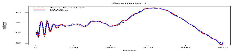
(a) Scenario 1, $n=500$

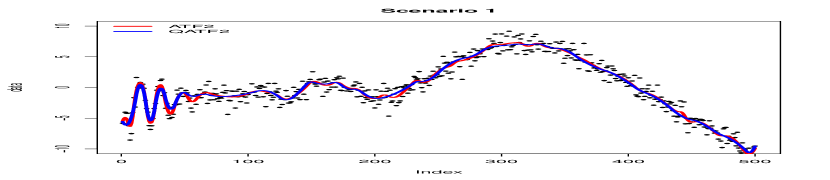
(b) Scenario 1, $n=500$

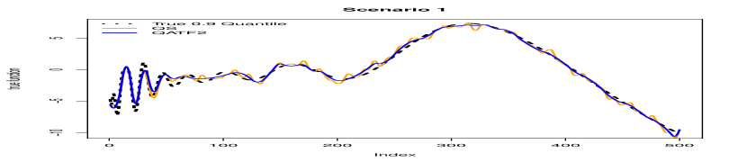
(c) Scenario 1, $n=500$

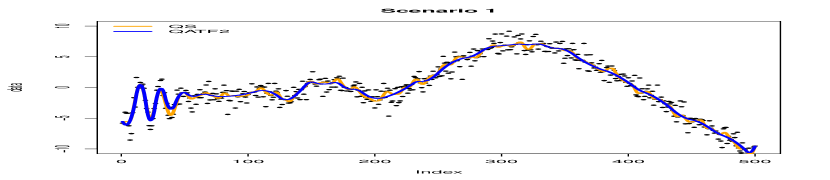
(d) Scenario 1, $n=500$

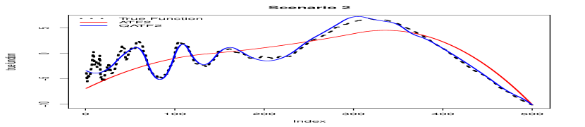
(e) Scenario 2, $n=500$

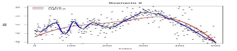
(f) Scenario 2, $n=500$

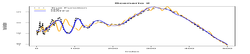
(g) Scenario 2, $n=500$

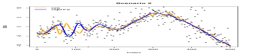
(h) Scenario 2, $n=500$

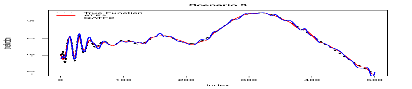
(i) Scenario 3, $n=500$

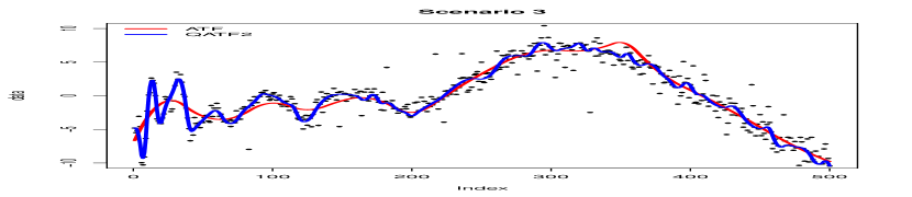
(j) Scenario 3, $n=500$

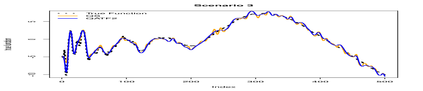
(k) Scenario 3, $n=500$

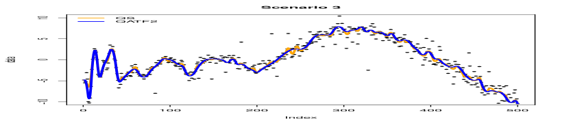
(l) Scenario 3, $n=500$

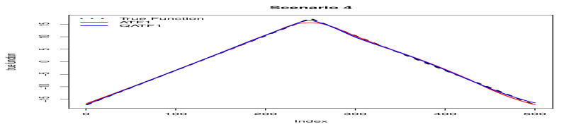
(m) Scenario 4, $n=500$

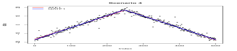
(n) Scenario 4, $n=500$

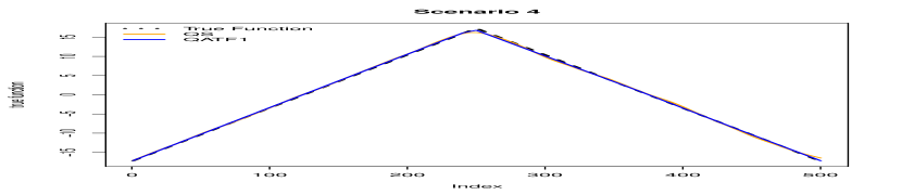
(o) Scenario 4, $n=500$

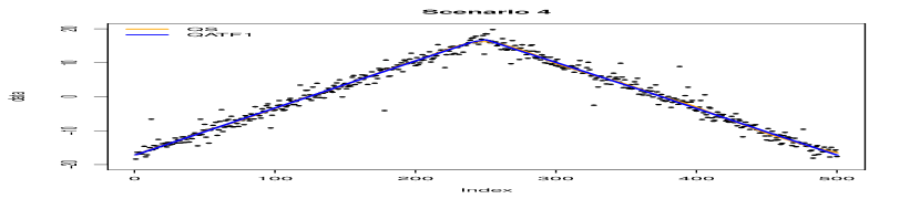
(p) Scenario 4, $n=500$

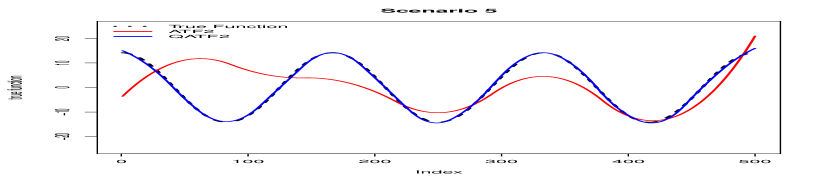
(q) Scenario 5, $n=500$

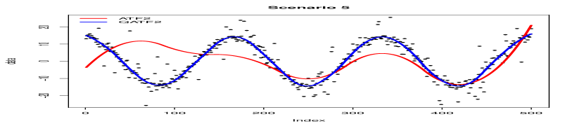
(r) Scenario 5, $n=500$

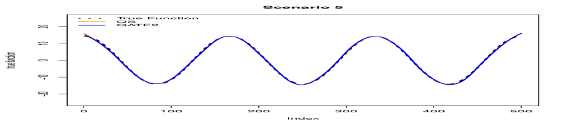
(s) Scenario 5, $n=500$

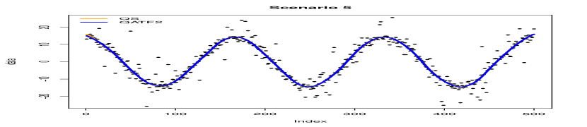
(t) Scenario 5, $n=500$

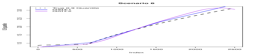
(u) Scenario 6, $n=500$

(v) Scenario 6, $n=500$

Figure 3: The plots in rows 1 to 6 correspond to scenarios 1 to 6. Figures 3(a),3(e), 3(i), 3(m), 3(q) plot QATF + ATF on the true function $f^{*}$. Figures 3(b),3(f), 3(j), 3(n), 3(r) plot QATF + ATF on real data. Figures 3(c),3(g), 3(k), 3(o), 3(s) plot QATF + QS on the true function $f^{*}$. Figures 3(d),3(h), 3(l), 3(p), 3(t) plot QATF + QS on real data. Figure 3(u) plots QATF1 + QATF2 on the true 0.9 quantile and 3(v) plots QATF1 + QS on the true 0.9 quantile.

References

Bartlett et al. (2005)
Peter L Bartlett, Olivier Bousquet, and Shahar Mendelson.
Local rademacher complexities.
2005.
Belloni and Chernozhukov (2011)
Alexandre Belloni and Victor Chernozhukov.
l 1-penalized quantile regression in high-dimensional sparse models.
2011.
Belloni et al. (2023)
Alexandre Belloni, Mingli Chen, Oscar Hernan Madrid Padilla, and Zixuan Wang.
High-dimensional latent panel quantile regression with an application
to asset pricing.
The Annals of Statistics, 51(1):96–121,
2023.
Benoit and Van den Poel (2009)
Dries F Benoit and Dirk Van den Poel.
Benefits of quantile regression for the analysis of customer lifetime
value in a contractual setting: An application in financial services.
Expert Systems with Applications, 36(7):10475–10484, 2009.
Birman and Solomyak (1967)
Mikhail Shlemovich Birman and Mikhail Zakharovich Solomyak.
Piecewise-polynomial approximations of functions of the classes
w_p^.
Matematicheskii Sbornik, 115(3):331–355,
1967.
Brantley et al. (2020)
Halley L Brantley, Joseph Guinness, and Eric C Chi.
Baseline drift estimation for air quality data using quantile trend
filtering.
2020.
Breiman and Friedman (1985)
Leo Breiman and Jerome H Friedman.
Estimating optimal transformations for multiple regression and
correlation.
Journal of the American statistical Association, 80(391):580–598, 1985.
Coad et al. (2006)
Alex Coad, Rekha Rao, et al.
Innovation and market value: a quantile regression analysis.
Economics Bulletin, 15(13):1–10, 2006.
Cox (1972)
David R Cox.
Regression models and life-tables.
Journal of the Royal Statistical Society: Series B
(Methodological), 34(2):187–202, 1972.
Dudley (1967)
Richard M Dudley.
The sizes of compact subsets of hilbert space and continuity of
gaussian processes.
Journal of Functional Analysis, 1(3):290–330, 1967.
Friedman and Stuetzle (1981)
Jerome H Friedman and Werner Stuetzle.
Projection pursuit regression.
Journal of the American statistical Association, 76(376):817–823, 1981.
Hastie and Tibshirani (1987)
Trevor Hastie and Robert Tibshirani.
Non-parametric logistic and proportional odds regression.
Journal of the Royal Statistical Society: Series C (Applied
Statistics), 36(3):260–276, 1987.
Hastie (2017)
Trevor J Hastie.
Generalized additive models.
In Statistical models in S, pages 249–307. Routledge, 2017.
Huber (1992)
Peter J Huber.
Robust estimation of a location parameter.
In Breakthroughs in statistics: Methodology and distribution,
pages 492–518. Springer, 1992.
Koenker (2011)
Roger Koenker.
Additive models for quantile regression: Model selection and
confidence bandaids.
2011.
Koenker et al. (1994)
Roger Koenker, Pin Ng, and Stephen Portnoy.
Quantile smoothing splines.
Biometrika, 81(4):673–680, 1994.
Lin and Zhang (2006)
Yi Lin and Hao Helen Zhang.
Component selection and smoothing in multivariate nonparametric
regression.
2006.
Lou et al. (2016)
Yin Lou, Jacob Bien, Rich Caruana, and Johannes Gehrke.
Sparse partially linear additive models.
Journal of Computational and Graphical Statistics, 25(4):1126–1140, 2016.
Madrid Padilla and Chatterjee (2022)
Oscar Hernan Madrid Padilla and Sabyasachi Chatterjee.
Risk bounds for quantile trend filtering.
Biometrika, 109(3):751–768, 2022.
Meier et al. (2009)
Lukas Meier, Sara Van de Geer, and Peter Bühlmann.
High-dimensional additive modeling.
2009.
Pata and Schindler (2015)
Petr Pata and Jaromir Schindler.
Astronomical context coder for image compression.
Experimental Astronomy, 39:495–512, 2015.
Perlich et al. (2007)
Claudia Perlich, Saharon Rosset, Richard D Lawrence, and Bianca Zadrozny.
High-quantile modeling for customer wallet estimation and other
applications.
In Proceedings of the 13th ACM SIGKDD international conference
on Knowledge discovery and data mining, pages 977–985, 2007.
Petersen et al. (2016)
Ashley Petersen, Daniela Witten, and Noah Simon.
Fused lasso additive model.
Journal of Computational and Graphical Statistics, 25(4):1005–1025, 2016.
Ravikumar et al. (2009)
Pradeep Ravikumar, John Lafferty, Han Liu, and Larry Wasserman.
Sparse additive models.
Journal of the Royal Statistical Society: Series B (Statistical
Methodology), 71(5):1009–1030, 2009.
Rudin et al. (1992)
Leonid I Rudin, Stanley Osher, and Emad Fatemi.
Nonlinear total variation based noise removal algorithms.
Physica D: nonlinear phenomena, 60(1-4):259–268, 1992.
Sadhanala and Tibshirani (2017)
Veeranjaneyulu Sadhanala and Ryan J Tibshirani.
Additive models with trend filtering.
arXiv preprint arXiv:1702.05037, 2017.
Sadhanala et al. (2016)
Veeranjaneyulu Sadhanala, Yu-Xiang Wang, and Ryan J Tibshirani.
Total variation classes beyond 1d: Minimax rates, and the limitations
of linear smoothers.
Advances in Neural Information Processing Systems, 29, 2016.
Sanderson et al. (2006)
Alastair JR Sanderson, Trevor J Ponman, and Ewan O’Sullivan.
A statistically selected chandra sample of 20 galaxy clusters–i.
temperature and cooling time profiles.
Monthly Notices of the Royal Astronomical Society,
372(4):1496–1508, 2006.
Shen et al. (2022)
Guohao Shen, Yuling Jiao, Yuanyuan Lin, Joel L Horowitz, and Jian Huang.
Estimation of non-crossing quantile regression process with deep requ
neural networks.
arXiv preprint arXiv:2207.10442, 2022.
Tibshirani (2014)
Ryan J Tibshirani.
Adaptive piecewise polynomial estimation via trend filtering.
2014.
Tseng (2001)
Paul Tseng.
Convergence of a block coordinate descent method for
nondifferentiable minimization.
Journal of optimization theory and applications, 109:475–494, 2001.
Wainwright (2019)
Martin J Wainwright.
High-dimensional statistics: A non-asymptotic viewpoint,
volume 48.
Cambridge university press, 2019.
Wang et al. (2015)
Yu-Xiang Wang, James Sharpnack, Alex Smola, and Ryan Tibshirani.
Trend filtering on graphs.
In Artificial Intelligence and Statistics, pages 1042–1050.
PMLR, 2015.
Wasko and Sharma (2014)
Conrad Wasko and Ashish Sharma.
Quantile regression for investigating scaling of extreme
precipitation with temperature.
Water Resources Research, 50(4):3608–3614, 2014.