A Comprehensive Survey on Vector Database: Storage and Retrieval Technique, Challenge

Abstract

A vector database is used to store high-dimensional data that cannot be characterized by traditional DBMS. Although there are not many articles describing existing or introducing new vector database architectures, the approximate nearest neighbor search problem behind vector databases has been studied for a long time, and considerable related algorithmic articles can be found in the literature. This article attempts to comprehensively review relevant algorithms to provide a general understanding of this booming research area. The basis of our framework categorises these studies by the approach of solving ANNS problem, respectively hash-based, tree-based, graph-based and quantization-based approaches. Then we present an overview of existing challenges for vector databases. Lastly, we sketch how vector databases can be combined with large language models and provide new possibilities.

I Introduction

Vector database is a type of database that stores data as high-dimensional vectors, which are mathematical representations of features or attributes. Each vector has a certain number of dimensions, which can range from tens to thousands, depending on the complexity and granularity of the data.

The vectors are usually generated by applying some kind of transformation or embedding function to the raw data, such as text, images, audio, video, and others. The embedding function can be based on various methods, such as machine learning models, word embeddings, feature extraction algorithms.

Vector databases have several advantages over traditional databases.

Fast and accurate similarity search and retrieval. Vector database can find the most similar or relevant data based on their vector distance or similarity, which is a core functionality for many applications that involve natural language processing, computer vision, recommendation systems, etc. Traditional database can only query data based on exact matches or predefined criteria, which may not capture the semantic or contextual meaning of the data.

Support for complex and unstructured data. Vector database can store and search data that have high complexity and granularity, such as text, images, audio, video, etc. These types of data are usually unstructured and do not fit well into the rigid schema of traditional database. Vector database can transform these data into high-dimensional vectors that can capture their features or attribute.

Scalability and performance. Vector database can handle large-scale and real-time data analysis and processing, which are essential for modern data science and AI applications. Vector database can use techniques such as sharding, partitioning, caching, replication, etc. to distribute the workload and optimize the resource utilization across multiple machines or clusters. Traditional database may face challenges such as scalability bottlenecks, latency issues, or concurrency conflicts when dealing with big data.

II Storage

II-A Sharding

Sharding is a technique that distributes a vector database across multiple machines or clusters, called shards, based on some criteria, such as a hash function or a key range. Sharding can improve the scalability, availability, and performance of vector database.

One way that sharding works in vector database is by using a hash-based sharding method, which assigns vector data to different shards based on the hash value of a key column or a set of columns. For example, users can shard a vector database by applying a hash function to the ID column of the vector data. This way, users can distribute the vector data evenly across the shards and avoid hotspots.

Another way that sharding works in vector database is by using a range-based sharding method, which assigns vector data to different shards based on the value ranges of a key column or a set of columns. For example, users can shard a vector database by dividing the ID column of the vector data into different ranges, such as 0-999, 1000-1999, 2000-2999, etc. Each range corresponds to a shard. This way, users can query the vector data more efficiently by specifying the shard name or range.

II-B Partitioning

Partitioning is a technique that divides a vector database into smaller and manageable pieces, called partitions, based on some criteria, such as geographic location, category, or frequency. Partitioning can improve the performance, scalability, and usability of vector database.

One way that partitioning works in vector database is by using a range partitioning method, which assigns vector data to different partitions based on their value ranges of a key column or a set of columns. For example, users can partition a vector database by date ranges, such as monthly or quarterly. This way, users can query the vector data more efficiently by specifying the partition name or range.

Another way that partitioning works in vector database is by using a list partitioning method, which assigns vector data to different partitions based on their value lists of a key column or a set of columns. For example, users can partition a vector database by color values, such as red, yellow, and blue. Each partition contains vector data that have a given value of the color column. This way, users can query the vector data more easily by specifying the partition name or list.

II-C Caching

Caching is a technique that stores frequently accessed or recently used data in a fast and accessible memory, such as RAM, to reduce the latency and improve the performance of data retrieval. Caching can be used in vector database to speed up the similarity search and retrieval of vector data.

One way that caching works in vector database is by using a least recently used (LRU) policy, which evicts the least recently used vector data from the cache when it is full. This way, the cache can store the most relevant or popular vector data that are likely to be queried again. For example, Redis, a popular in-memory database, uses LRU caching to store vector data and support vector similarity search.

Another way that caching works in vector database is by using a partitioned cache, which divides the vector data into different partitions based on some criteria, such as geographic location, category, or frequency. Each partition can have its own cache size and eviction policy, depending on the demand and usage of the vector data. This way, the cache can store the most appropriate vector data for each partition and optimize the resource utilization. For example, Esri, a geographic information system (GIS) company, uses partitioned cache to store vector data and support map rendering.

II-D Replication

Replication is a technique that creates multiple copies of the vector data and stores them on different nodes or clusters. Replication can improve the availability, durability, and performance of vector database.

One way that replication works in vector database is by using a leaderless replication method, which does not distinguish between primary and secondary nodes, and allows any node to accept write and read requests. Leaderless replication can avoid single points of failure and improve the scalability and reliability of vector database. However, it may also introduce consistency issues and require coordination mechanisms to resolve conflicts.

Another way that replication works in vector database is by using a leader-follower replication method, which designates one node as the leader and the others as the followers, and allows only the leader to accept write requests and propagate them to the followers. Leader-follower replication can ensure strong consistency and simplify the conflict resolution of vector database. However, it may also introduce availability issues and require failover mechanisms to handle leader failures.

III Search

Nearest neighbor search (NNS) is the optimization problem of finding the point in a given set that is closest (or most similar) to a given point. Closeness is typically expressed in terms of a dissimilarity function: the less similar the objects, the larger the function values. For example, users can use NNS to find images that are similar to a given image based on their visual content and style, or documents that are similar to a given document based on their topic and sentiment.

Approximate nearest neighbor search (ANNS) is a variation of NNS that allows for some error or approximation in the search results. ANNS can trade off accuracy for speed and space efficiency, which can be useful for large-scale and high-dimensional data. For example, users can use ANNS to find products that are similar to a given product based on their features and ratings, or users that are similar to a given user based on their preferences and behaviors.

Observing the current division for NNS and ANNS algorithms, the boundary is precisely their design principle, such as how they organize, index, or hash the dataset, how they search or traverse the data structure, and how they measure or estimate the distance between points. NNS algorithms tend to use more exact or deterministic methods, such as partitioning the space into regions by splitting along one dimension (k-d tree) or enclosing groups of points in hyperspheres (ball tree), and visiting only the regions that may contain the nearest neighbor based on some distance bounds or criteria. ANNS algorithms tend to use more probabilistic or heuristic methods, such as mapping similar points to the same or nearby buckets with high probability (locality-sensitive hashing), visiting the regions in order of their distance to the query point and stopping after a fixed number of regions or points (best bin first), or following the edges that lead to closer points in a graph with different levels of coarseness (hierarchical navigable small world).

In fact, a data structure or algorithm can support ANNS if it is applicable to NNS. For ease of categorization, it is assigned to the section on Nearest Neighbor Search.

III-A Nearest Neighbor Search

III-A1 Brute Force Approach

A brute force algorithm for NNS problem is a very simple and naive algorithm, which scans through all the points in the dataset and computes the distance to the query point, keeping track of the best so far. This algorithm guarantees to find the true nearest neighbor for any query point, but it has a high computational cost. The time complexity of a brute force algorithm for NNS problem is $O(n)$, where n is the size of the dataset. The space complexity is $O(1)$, since no extra space is needed.

III-A2 Tree-Based Approach

Four tree-based methods will be presented here, namely KD-tree, Ball-tree, R-tree, and M-tree.

KD-tree [1]. It is a technique for organizing points in a k-dimensional space, where k is usually a very big number. It works by building a binary tree in which every node is a k-dimensional point. Every non-leaf node in the tree acts as a splitting hyperplane that divides the space into two parts, known as half-spaces. The splitting hyperplane is perpendicular to the chosen axis, which is associated with one of the k dimensions. The splitting value is usually the median or the mean of the points along that dimension.

The algorithm maintains a priority queue of nodes to visit, sorted by their distance to the query point. At each step, the algorithm pops the node with the smallest distance from the queue, and checks if it is a leaf node or an internal node. If it is a leaf node, the algorithm compares the distance between the query point and the data point stored in the node, and updates the current best distance and nearest neighbor if necessary. If it is an internal node, the algorithm pushes its left and right children to the queue, with their distances computed as follows:

$$\begin{array}[]{l}d_{L}(q,N)=\left\{\begin{array}[]{cc}0&\text{ if }q_{N.axis}\leq N.value\\ \left(q_{{N.axis}}-{N.value}\right)^{2}&\text{ if }q_{{N.axis}}>{N.value}\end{array}\right.\\ d_{R}(q,N)=\left\{\begin{array}[]{cc}0&\text{ if }q_{{N.axis}}\geq{N.value}\\ \left({N.value}-q_{{N.axis}}\right)^{2}&\text{ if }q_{{N.axis}}<{N.value}\end{array}\right.\end{array}$$ (1)

where $q$ is the query point, $N$ is the internal node, $N.axis$ is the splitting axis of $N$, and $N.value$ is the splitting value of $N$. The algorithm repeats this process until the queue is empty or a termination condition is met.

The advantage of KD-tree is that it is conceptually simpler and often easier to implement than some of the other tree structures.

The performance of KD-tree depends on several factors, such as the dimensionality of the space, the number of points, and the distribution of the points. These factors affect the trade-off between accuracy and efficiency, as well as the complexity and scalability of the algorithm. There are also some challenges and extensions of KD-tree, such as dealing with the curse of dimensionality when the dimensionality is high, introducing randomness in the splitting process to improve robustness, or using multiple trees to increase recall. This is a variation of KD-tree named randomized KD-tree, that introduces some randomness in the splitting process, which can improve the performance of KD-tree by reducing its sensitivity to noise and outliers [2].

Ball-tree [3], [4], [5]. It is a technique for finding the nearest neighbors of a given vector in a large collection of vectors. It works by building a ball-tree, which is a binary tree that partitions the data points into balls, i.e. hyperspheres that contain a subset of the points. Each node of the ball-tree defines the smallest ball that contains all the points in its subtree. The algorithm then searches for the closest ball to the query point, and then searches within the closest ball to find the closest point to the query point.

To query for the nearest neighbor of a given point, the ball tree algorithm uses a priority queue to store the nodes to be visited, sorted by their distance to the query point. The algorithm starts from the root node and pushes its two children to the queue. Then, it pops the node with the smallest distance from the queue and checks if it is a leaf node or an internal node. If it is a leaf node, it computes the distance between the query point and each data point in the node, and updates the current best distance and nearest neighbor if necessary. If it is an internal node, it pushes its two children to the queue, with their distances computed as follows:

$$\begin{array}[]{l}d_{L}(q,N)=\max(0,{N.value}-\|q-{N.center}\|)\\ d_{R}(q,N)=\max(0,\|q-{N.center}\|-N.value)\end{array}$$ (2)

where $q$ is the query point, $N$ is the internal node, $N.center$ is the center of the ball associated with $N$, and $N.value$ is the radius of the ball associated with $N$. The algorithm repeats this process until the queue is empty or a termination condition is met.

The advantage of ball-tree is that it can perform well in high-dimensional spaces, as it can avoid the curse of dimensionality that affects other methods such as KD-tree.

The performance of ball-tree depends on several factors, such as the dimensionality of the data, the number of balls per node, and the distance approximation method used. These factors affect the trade-off between accuracy and efficiency, as well as the complexity and scalability of the algorithm. There are also some challenges and extensions of ball-tree search, such as dealing with noisy and outlier data, choosing a good splitting dimension and value for each node, or using multiple trees to increase recall.

R-tree [6]. It is a technique for finding the nearest neighbors of a given vector in a large collection of vectors. It works by building an R-tree, which is a tree data structure that partitions the data points into rectangles, i.e. hyperrectangles that contain a subset of the points. Each node of the R-tree defines the smallest rectangle that contains all the points in its subtree. The algorithm then searches for the closest rectangle to the query point, and then searches within the closest rectangle to find the closest point to the query point.

The R-tree algorithm uses the concept of minimum bounding rectangle (MBR) to represent the spatial objects in the tree. The MBR of a set of points is the smallest rectangle that contains all the points. The formula for computing the MBR of a set of points $P$ is:

$$MBR(P)=\left[\min_{p\in P}p_{x},\max_{p\in P}p_{x}\right]\times\left[\min_{p\in P}p_{y},\max_{p\in P}p_{y}\right]$$ (3)

where $p_{x}$ and $p_{y}$ are the $\mathrm{x}$ and $\mathrm{y}$ coordinates of point $p$ , and $\times$ denotes the Cartesian product.

The R-tree algorithm also uses two metrics to measure the quality of a node split: area and overlap. The area of a node is the area of its MBR, and the overlap of two nodes is the area of the intersection of their MBRs. The formula for computing the area of a node N is:

$$\operatorname{area}(N)=\left(N.x_{\max}-N.x_{\min}\right)\times\left(N\cdot y_{\max}-N\cdot y_{\min}\right)$$ (4)

where $N.x_{\min}$, $N.x_{\max}$, $N.y_{\min}$, and $N.y_{\max}$ are the coordinates of the MBR of node $N$.

The advantage of R-tree is that it can support spatial queries, such as range queries or nearest neighbor queries, on data points that represent geographical coordinates, rectangles, polygons, or other spatial objects.

R-tree search performance depends on roughly the same factors as B-tree, and also faces similar challenges as B-tree.

M-tree [7]. It is a technique for finding the nearest neighbors of a given vector in a large collection of vectors. It works by building an M-tree, which is a tree data structure that partitions the data points into balls, i.e. hyperspheres that contain a subset of the points. Each node of the M-tree defines the smallest ball that contains all the points in its subtree. The algorithm then searches for the closest ball to the query point, and then searches within the closest ball to find the closest point to the query point.

The M-tree algorithm uses the concept of covering radius to represent the spatial objects in the tree. The covering radius of a node is the maximum distance from the node’s routing object to any of its children objects. The formula for computing the covering radius of a node $N$ is:

$$r(N)=\max_{C\in N.child}d(N.object,C.object)$$ (5)

where $N.object$ is the routing object of node $N$, $N.child$ is the set of child nodes of node $N$, $C.object$ is the routing object of child node $C$, and $d$ is the distance function.

The M-tree algorithm also uses two metrics to measure the quality of a node split: area and overlap. The area of a node is the sum of the areas of its children’s covering balls, and the overlap of two nodes is the sum of the areas of their children’s overlapping balls. The formula for computing the area of a node $N$ is:

$$\operatorname{area}(N)=\sum_{C\in\text{ N.child }}\pi r(C)^{2}$$ (6)

where $\pi$ is the mathematical constant, and $r(C)$ is the covering radius of child node $C$.

The advantage of M-tree is that it can support dynamic operations, such as inserting or deleting data points, by updating the tree structure accordingly.

M-tree search performance depends on roughly the same factors as B-tree, and also faces similar challenges as B-tree.

III-B Approximate Nearest Neighbor Search

III-B1 Hash-Based Approach

Three hash-based methods will be presented here, namely local-sensitive hashing, spectral hashing, and deep hashing. The idea is to reduce the memory footprint and the search time by comparing the binary codes instead of the original vectors [8].

Local-sensitive hashing [9]. It is a technique for finding the approximate nearest neighbors of a given vector in a large collection of vectors. It works by using a hash function to transform the high-dimensional vectors into compact binary codes, and then using a hash table to store and retrieve the codes based on their similarity or distance. The hash function is designed to preserve the locality of the vectors, meaning that similar vectors are more likely to have the same or similar codes than dissimilar vectors. Jafari et al. [10] conduct a survey on local-sensitive hashing. A trace of algorithm description and implementation for locally sensitive hashing can be seen on the home page [11].

The LSH algorithm works by using a family of hash functions that use random projections or other techniques which are locality sensitive, meaning that similar vectors are more likely to have the same or similar codes than dissimilar vectors [dikkala2021manifold], which satisfy the following property:

$$\operatorname{Pr}[h(p)=h(q)]=f(d(p,q))$$ (7)

where $h$ is a hash function, $p$ and $q$ are two points, $d$ is a distance function, and $f$ is a similarity function. The similarity function $f$ is a monotonically decreasing function of the distance, such that the closer the points are, the higher the probability of collision.

There are different families of hash functions for different distance functions and similarity functions. For example, one of the most common families of hash functions for Euclidean distance and cosine similarity is:

$$h(p)=\left\lfloor\frac{a\cdot p+b}{w}\right\rfloor$$ (8)

where $a$ is a random vector, $b$ is a random scalar, and $w$ is a parameter that controls the size of the hash bucket. The similarity function for this family of hash functions is:

$$f(d(p,q))=1-\frac{d(p,q)}{\pi w}$$ (9)

where $d(p,q)$ is the Euclidean distance between $p$ and $q$.

The advantage of LSH is that it can reduce the memory footprint and the search time by comparing the binary codes instead of the original vectors, also adapt to dynamic data sets, by inserting or deleting codes from the hash table without affecting the existing codes [12].

The performance of LSH depends on several factors, such as the dimensionality of the data, the number of hash functions, the number of bits per code, and the desired accuracy and recall. These factors affect the trade-off between accuracy and efficiency, as well as the complexity and scalability of the algorithm. There are also some challenges and extensions of LSH, such as dealing with noisy and outlier data, choosing a good hash function family, or using multiple hash tables to increase recall. It is improved by [13], [14], [15].

Spectral hashing [16]. It is a technique for finding the approximate nearest neighbors of a given vector in a large collection of vectors. It works by using spectral graph theory to generate hash functions that minimize the quantization error and maximize the variance of the binary codes. Spectral hashing can perform well when the data points lie on a low-dimensional manifold embedded in a high-dimensional space.

The spectral hashing algorithm works by solving an optimization problem that balances two objectives: (1) minimizing the variance of each binary function, which ensures that the data points are evenly distributed among the hypercubes, and (2) maximizing the mutual information between different binary functions, which ensures that the binary code is informative and discriminative. The optimization problem can be formulated as follows:

$$\min_{y_{1},\ldots,y_{n}}\sum_{i=1}^{n}Var\left(y_{i}\right)-\lambda I\left(y_{1},\ldots,y_{n}\right)$$ (10)

where $y_{i}$ is the $i$-th binary function, $Var\left(y_{i}\right)$ is its variance, $I\left(y_{1},\ldots,y_{n}\right)$ is the mutual information between all the binary functions, and $\lambda$ is a trade-off parameter.

The advantage of spectral hashing is that it can perform well when the data points lie on a low-dimensional manifold embedded in a high-dimensional space.

Spectral hashing search performance depends on roughly the same factors as local-sensitive hashing. There are also some challenges and extensions of spectral hashing, such as dealing with noisy and outlier data, choosing a good graph Laplacian for the data manifold, or using multiple hash functions to increase recall.

Deep hashing [17]. It is a technique for finding the approximate nearest neighbors of a given vector in a large collection of vectors. It works by using a deep neural network to learn hash functions that transform the high-dimensional vectors into compact binary codes, and then using a hash table to store and retrieve the codes based on their similarity or distance. The hash functions are designed to preserve the semantic information of the vectors, meaning that similar vectors are more likely to have the same or similar codes than dissimilar vectors [18]. Luo et al. [19] conduct a survey on deep hashing.

The deep hashing algorithm works by optimizing an objective function that balances two terms: (1) a reconstruction loss that measures the fidelity of the binary codes to the original data points, and (2) a quantization loss that measures the discrepancy between the binary codes and their continuous relaxations. The objective function can be formulated as follows:

$$\min_{W,B}\sum_{i=1}^{N}\left\|x_{i}-Wb_{i}\right\|_{2}^{2}+\lambda\left\|b_{i}-\operatorname{sgn}\left(b_{i}\right)\right\|_{2}^{2}$$ (11)

where $x_{i}$ is the $i$-th data point, $b_{i}$ is its continuous relaxation, $\operatorname{sgn}\left(b_{i}\right)$ is its binary code, $W$ is a weight matrix that maps the binary codes to the data space, and $\lambda$ is a trade-off parameter.

The advantage of deep hashing is that it can leverage the representation learning ability of neural networks to generate more discriminative and robust codes for complex data, such as images, texts, or audios.

The performance of deep hashing depends on several factors, such as the architecture of the neural network, the loss function used to train the network, and the number of bits per code. These factors affect the trade-off between accuracy and efficiency, as well as the complexity and scalability of the algorithm. There are also some challenges and extensions of deep hashing, such as dealing with noisy and outlier data, choosing a good initialization for the network, or using multiple hash functions to increase recall.

III-B2 Tree-Based Approach

Three tree-based methods will be presented here, namely approximate nearest neighbors oh yeah, best bin first, and k-means tree. The idea is to reduce the search space by following the branches of the tree that are most likely to contain the nearest neighbors of the query point.

Approximate Nearest Neighbors Oh Yeah [20]. It is a technique which can perform fast and accurate similarity search and retrieval of high-dimensional vectors. It works by building a forest of binary trees, where each tree splits the vector space into two regions based on a random hyperplane. Each vector is then assigned to a leaf node in each tree based on which side of the hyperplane it falls on. To query a vector, Annoy traverses each tree from the root to the leaf node that contains the vector, and collects all the vectors in the same leaf nodes as candidates. Then, it computes the exact distance or similarity between the query vector and each candidate, and returns the top $k$ nearest neighbors.

The formula for finding the median hyperplane between two points $p$ and $q$ is:

$$w\cdot x+b=0$$ (12)

where $w=p-q$ is the normal vector of the hyperplane, $x$ is any point on the hyperplane, and $b=-\frac{1}{2}(w\cdot p+w\cdot q)$ is the bias term.

The formula for assigning a point x to a leaf node in a tree is:

$$\operatorname{sign}\left(w_{i}\cdot x+b_{i}\right)$$ (13)

where $w_{i}$ and $b_{i}$ are the normal vector and bias term of the $i$-th split in the tree, and sign is a function that returns $1$ if the argument is positive, $-1$ if negative, and $0$ if zero. The point $x$ follows the left or right branch of the tree depending on the sign of this expression, until it reaches a leaf node.

The formula for searching for the nearest neighbor of a query point $q$ in the forest is:

$$\min_{x\in C(q)}d(q,x)$$ (14)

where $C(q)$ is the set of candidate points obtained by traversing each tree in the forest and retrieving all the points in the leaf node that $q$ belongs to, and $d$ is a distance function, such as Euclidean distance or cosine distance. The algorithm uses a priority queue to store the nodes to be visited, sorted by their distance to $q$. The algorithm also prunes branches that are unlikely to contain the nearest neighbor by using a bound on the distance between $q$ and any point in a node.

The advantage of Annoy is that it can uses multiple random projection trees to index the data points, which can increase the recall and robustness of the search, also reduce the memory usage and improve the speed of nearest neighbor search, by creating large read-only file-based data structures that are mapped into memory so that many processes can share the same data.

The performance of Annoy depends on several factors, such as the dimensionality of the data, the number of trees built, the number of nearest candidates to search, and the distance approximation method used. These factors affect the trade-off between accuracy and efficiency, as well as the complexity and scalability of the algorithm. There are also some challenges and extensions of Annoy, such as dealing with noisy and outlier data, choosing a good splitting plane for each node, or using multiple distance metrics to increase recall.

Best bin first [21], [22]. It is a technique for finding the approximate nearest neighbors of a given vector in a large collection of vectors. It works by building a kd-tree that partitions the data points into bins, and then searching for the closest bin to the query point. The algorithm then searches within the closest bin to find the closest point to the query point.

The best bin first algorithm still follows (1).

The advantage of best bin first is that it can reduce the search time and improve the accuracy of nearest neighbor search, by focusing on the most promising bins and avoiding unnecessary comparisons with distant points.

The performance of best bin first depends on several factors, such as the dimensionality of the data, the number of bins per node, the number of nearest candidates to search, and the distance approximation method used. These factors affect the trade-off between accuracy and efficiency, as well as the complexity and scalability of the algorithm. There are also some challenges and extensions of best bin first, such as dealing with noisy and outlier data, choosing a good splitting dimension and value for each node, or using multiple trees to increase recall.

K-means tree [23]. It is a technique for clustering high-dimensional data points into a hierarchical structure, where each node represents a cluster of points. It works by applying a k-means clustering algorithm to the data points at each level of the tree, and then creating child nodes for each cluster. The process is repeated recursively until a desired depth or size of the tree is reached.

The formula for assigning a point $x$ to a cluster using the k-means algorithm is:

$$\mathop{\arg\min}_{i=1,\ldots,k}\left\|x-c_{i}\right\|_{2}^{2}$$ (15)

where argmin is a function that returns the argument that minimizes the expression, and $\|\cdot\|_{2}$ denotes the Euclidean norm.

The formula for assigning a point $x$ to a leaf node in a k-means tree is:

$$\mathop{\arg\min}_{N\in L(x)}\|x-N.center\|_{2}^{2}$$ (16)

where $L(x)$ is the set of leaf nodes that x belongs to, and N .center is the cluster center of node $N$. The point $x$ belongs to a leaf node if it belongs to all its ancestor nodes in the tree.

The formula for searching for the nearest neighbor of a query point $q$ in the k-means tree is:

$$\min_{x\in C(q)}\|q-x\|_{2}^{2}$$ (17)

where $C(q)$ is the set of candidate points obtained by traversing each branch of the tree and retrieving all the points in the leaf nodes that $q$ belongs to. The algorithm uses a priority queue to store the nodes to be visited, sorted by their distance to $q$. The algorithm also prunes branches that are unlikely to contain the nearest neighbor by using a bound on the distance between $q$ and any point in a node.

The advantage of K-means tree is that it can perform fast and accurate similarity search and retrieval of data points based on their cluster membership, by following the branches of the tree that are most likely to contain the nearest neighbors of the query point. K-means tree can also support dynamic operations, such as inserting and deleting points, by updating the tree structure accordingly.

The performance of K-means tree depends on several factors, such as the dimensionality of the data, the number of clusters per node, and the distance metric used. These factors affect the trade-off between accuracy and efficiency, as well as the complexity and scalability of the algorithm. There are also some challenges and extensions of K-means tree, such as dealing with noisy and outlier points, choosing a good initialization for the k-means algorithm, or using multiple trees to increase recall.

III-B3 Graph-Based Approach

Two graph-based methods will be presented here, namely navigable small world, and hierachical navigable small world.

Navigable small world [24], [25], [26]. It is a technique that uses a graph structure to store and retrieve high-dimensional vectors based on their similarity or distance. The NSW algorithm builds a graph by connecting each vector to its nearest neighbors, as well as some random long-range links that span different regions of the vector space. The idea is that these long-range links create shortcuts that allow for faster and more efficient traversal of the graph, similar to how social networks have small world properties.

The NSW algorithm works by using a greedy heuristic to add edges to the graph. The algorithm starts with an empty graph and adds one point at a time. For each point, the algorithm finds its nearest neighbor in the graph using a random walk, and connects it with an edge. Then, the algorithm adds more edges by connecting the point to other points that are closer than its current neighbors. The algorithm repeats this process until all points are added to the graph.

The formula for finding the nearest neighbor of a point p in the graph using a random walk is:

$$\mathop{\arg\min}_{q\in N(p)}d(p,q)$$ (18)

where N(p) is the set of neighbors of p in the graph, and d is a distance function, such as Euclidean distance or cosine distance. The algorithm starts from a random point in the graph and moves to its nearest neighbor until it cannot find a closer point. The formula for adding more edges to the graph using a greedy heuristic is:

$$\forall q\in N(p),\forall r\in N(q)\text{, if }d(p,r)<d(p,q)\text{, then add edge }(p,r)$$ (19)

where $N(p)$ and $N(q)$ are the sets of neighbors of $p$ and $q$ in the graph, respectively, and $d$ is a distance function. The algorithm connects $p$ to any point that is closer than its current neighbors.

The advantage of the NSW algorithm is that it can handle arbitrary distance metrics, it can adapt to dynamic data sets, and it can achieve high accuracy and recall with low memory consumption. The NSW algorithm also uses a greedy routing strategy, which means that it always moves to the node that is closest to the query vector, until it reaches a local minimum or a predefined number of hops.

The performance of the NSW algorithm depends on several factors, such as the dimensionality of the vectors, the number of neighbors per node, the number of long-range links per node, and the number of hops per query. These factors affect the trade-off between accuracy and efficiency, as well as the complexity and scalability of the algorithm. There are also some extensions and variations of the NSW algorithm, such as hierarchical navigable small world (HNSW), which adds multiple layers of graphs, each with different scales and densities, or navigable small world with pruning (NSWP), which removes redundant links to reduce memory usage and improve search speed.

Hierachical navigable small world [27]. It is a state-of-the-art technique for finding the approximate nearest neighbors of a given vector in a large collection of vectors. It works by building a graph structure that connects the vectors based on their similarity or distance, and then using a greedy search strategy to traverse the graph and find the most similar vectors.

The HNSW algorithm still follows (18) and (19).

The HNSW algorithm also builds a hierarchical structure of the graph by assigning each point to different layers with different probabilities. The higher layers contain fewer points and longer edges, while the lower layers contain more points and shorter edges. The highest layer contains only one point, which is the entry point for the search. The algorithm uses a parameter M to control the maximum number of neighbors for each point in each layer.

The formula for assigning a point $p$ to a layer $l$ using a random probability is:

$$\operatorname{Pr}[p\in l]=\left\{\begin{array}[]{cc}1&\text{ if }l=0\\ \frac{1}{M}&\text{ if }l>0\end{array}\right.$$ (20)

where $M$ is the parameter that controls the maximum number of neighbors for each point in each layer. The algorithm assigns $p$ to layer $l$ with probability $\operatorname{Pr}[p\in l]$, and stops when it fails to assign $p$ to any higher layer.

The formula for searching for the nearest neighbor of a query point q in the hierarchical graph is:

$$\min_{p\in C(q)}d(q,p)$$ (21)

where $C(q)$ is the set of candidate points obtained by traversing each layer of the graph from top to bottom and retrieving all the points that are closer than the current best distance. The algorithm uses a priority queue to store the nodes to be visited, sorted by their distance to $q$. The algorithm also prunes branches that are unlikely to contain the nearest neighbor by using a bound on the distance between $q$ and any point in a node.

The advantage of HNSW is that it can achieve better performance than other methods of approximate nearest neighbor search, such as tree-based or hash-based techniques. For example, it can handle arbitrary distance metrics, it can adapt to dynamic data sets, and it can achieve high accuracy and recall with low memory consumption. HNSW also uses a hierarchical structure that allows for fast and accurate search, by starting from the highest layer and moving down to the lowest layer, using the closest node as the next hop at each layer.

The performance of HNSW depends on several factors, such as the dimensionality of the vectors, the number of layers, the number of neighbors per node, and the number of hops per query. These factors affect the trade-off between accuracy and efficiency, as well as the complexity and scalability of the algorithm. There are also some challenges and extensions of HNSW, such as finding the optimal parameters for the graph construction, dealing with noise and outliers, and scaling to very large data sets. Some of the extensions include optimized product quantization (OPQ), which combines HNSW with product quantization to reduce quantization distortions, or product quantization network (PQN), which uses a neural network to learn an end-to-end product quantizer from data.

III-B4 Quantization-Based Approach

Three quantization-based methods will be presented here, namely product quantization, optimized product quantization, and online product quantization. Product quantization can reduce the memory footprint and the search time of ANN search, by comparing the codes instead of the original vectors [28].

Product quantization [29]. It is a technique for compressing high-dimensional vectors into smaller and more efficient representations. It works by dividing a vector into several sub-vectors, and then applying a clustering algorithm (such as k-means) to each sub-vector to assign it to one of a finite number of possible values (called centroids). The result is a compact code that consists of the indices of the centroids for each sub-vector.

The PQ algorithm works by using a vector quantization technique to map each subvector to its nearest centroid in a predefined codebook. The algorithm first splits each vector into $m$ equal-sized subvectors, where m is a parameter that controls the length of the code. Then, for each subvector, the algorithm learns $k$ centroids using the k-means algorithm, where $k$ is a parameter that controls the size of the codebook. Finally, the algorithm assigns each subvector to its nearest centroid and concatenates the centroid indices to form the code.

The formula for splitting a vector $x$ into $m$ subvectors is:

$$x=\left(x_{1},x_{2},\ldots,x_{m}\right)$$ (22)

where $x_{i}$ is the $i$-th subvector of $x$, and has dimension $d/m$, where $d$ is the dimension of $x$.

The formula for finding the centroids of a set of subvectors $P$ using the k-means algorithm is:

$$c_{i}=\frac{1}{\left|S_{i}\right|}\sum_{x\in S_{i}}x$$ (23)

where $c_{i}$ is the $i$-th centroid, $S_{i}$ is the set of subvectors assigned to the i -th cluster, and $|\cdot|$ denotes the cardinality of a set.

The formula for assigning a subvector $x$ to a centroid using the k-means algorithm is:

$$\operatorname{argmin}_{i=1,\ldots,k}\left\|x-c_{i}\right\|_{2}^{2}$$ (24)

where argmin is a function that returns the argument that minimizes the expression, and $\|\cdot\|_{2}$ denotes the Euclidean norm.

The formula for encoding a vector $x$ using PQ is:

$$c(x)=\left(q_{1}\left(x_{1}\right),q_{2}\left(x_{2}\right),\ldots,q_{m}\left(x_{m}\right)\right)$$ (25)

where $x_{i}$ is the $i$-th subvector of $x$, and $q_{i}$ is the quantization function for the $i$-th subvector, which returns the index of the nearest centroid in the codebook.

The advantage of product quantization is that it is simple and easy to implement, as it only requires a standard clustering algorithm and a simple distance approximation method.

The performance of product quantization depends on several factors, such as the dimensionality of the data, the number of sub-vectors, the number of centroids per sub-vector, and the distance approximation method used. These factors affect the trade-off between accuracy and efficiency, as well as the complexity and scalability of the algorithm. There are also some challenges and extensions of product quantization, such as dealing with noisy and outlier data, optimizing the space decomposition and the codebooks, or adapting to dynamic data sets.

Optimized product quantization [30]. It is a variation of product quantization (PQ), which is a technique for compressing high-dimensional vectors into smaller and more efficient representations. OPQ works by optimizing the space decomposition and the codebooks to minimize quantization distortions. OPQ can improve the performance of PQ by reducing the loss of information and increasing the discriminability of the codes [31].

The advantage of OPQ is that it can achieve higher accuracy and recall than PQ, as it can better preserve the similarity or distance between the original vectors.

The formula for applying a random rotation to the data is:

$$x^{\prime}=Rx$$ (26)

where $x$ is the original vector, $x^{\prime}$ is the rotated vector, and $R$ is a random orthogonal matrix. The formula for finding the rotation matrix for a subvector using an optimization technique is:

$$\min_{R_{i}}\sum_{x\in P_{i}}\left\|x-R_{i}c_{i}\left(R_{i}x\right)\right\|_{2}^{2}$$ (27)

where $P_{i}$ is the set of subvectors assigned to the $i$-th cluster, $R_{i}$ is the rotation matrix for the $i$-th cluster, and $c_{i}$ is the quantization function for the $i$-th cluster, which returns the nearest centroid in the codebook.

The formula for encoding a vector $x$ using OPQ is:

$$c(x)=\left(q_{1}\left(R_{1}x_{1}\right),q_{2}\left(R_{2}x_{2}\right),\ldots,q_{m}\left(R_{m}x_{m}\right)\right)$$ (28)

where $x_{i}$ is the $i$-th subvector of $x$, $R_{i}$ is the rotation matrix for the $i$ -th subvector, and $q_{i}$ is the quantization function for the $i$-th subvector, which returns the index of the nearest centroid in the codebook.

The performance of OPQ depends on several factors, such as the dimensionality of the data, the number of sub-vectors, the number of centroids per sub-vector, and the distance approximation method used. These factors affect the trade-off between accuracy and efficiency, as well as the complexity and scalability of the algorithm. There are also some challenges and extensions of OPQ, such as dealing with noisy and outlier data, choosing a good optimization algorithm, or combining OPQ with other techniques such as hierarchical navigable small world (HNSW) or product quantization network (PQN).

Online product quantization [32]. It is a variation of product quantization (PQ), which is a technique for compressing high-dimensional vectors into smaller and more efficient representations. O-PQ works by adapting to dynamic data sets, by updating the quantization codebook and the codes online. O-PQ can handle data streams and incremental data sets, without requiring offline retraining or reindexing.

The formula for splitting a vector $x$ into $m$ subvectors is:

$$x=\left(x_{1},x_{2},\ldots,x_{m}\right)$$ (29)

where $x_{i}$ is the $i$-th subvector of $x$, and has dimension $d/m$, where $d$ is the dimension of $x$.

The formula for initializing the centroids of a set of subvectors $P$ using the k-means++ algorithm is:

$$c_{i}=\text{ randomly choose a point from }P$$ (30)

where $c_{i}$ is the $i$-th centroid, with probability proportional to $D(x)^{2}$, $D(x)$ is the distance between point $x$ and its closest centroid among $\left\{c_{1},\ldots,c_{i-1}\right\}$.

The formula for assigning a subvector $x$ to a centroid using $\mathrm{PQ}$ is:

$$\operatorname{argmin}_{i=1,\ldots,k}\left\|x-c_{i}\right\|_{2}^{2}$$ (31)

where $\arg\min$ is a function that returns the argument that minimizes the expression, and $\|\cdot\|_{2}$ denotes the Euclidean norm.

The formula for encoding a vector $x$ using $\mathrm{PQ}$ is:

$$c(x)=\left(q_{1}\left(x_{1}\right),q_{2}\left(x_{2}\right),\ldots,q_{m}\left(x_{m}\right)\right)$$ (32)

where $x_{i}$ is the $i$-th subvector of $x$, and $q_{i}$ is the quantization function for the $i$-th subvector, which returns the index of the nearest centroid in the codebook.

The O-PQ algorithm also updates the codebooks and codes for each subvector using an online learning technique. The algorithm uses two parameters: $\alpha$, which controls the learning rate, and $\beta$, which controls the forgetting rate. The algorithm updates the codebooks and codes as follows:

For each new point $x$, assign it to its nearest centroid in each subvector using PQ.

For each subvector $x_{i}$, update its centroid $c_{q_{i}\left(x_{i}\right)}$ as:

$$c_{q_{i}\left(x_{i}\right)}=(1-\alpha)c_{q_{i}\left(x_{i}\right)}+\alpha x_{i}$$ (33)

For each subvector $x_{i}$, update its code $q_{i}\left(x_{i}\right)$ as:

$$q_{i}\left(x_{i}\right)=\arg\min_{j=1,\ldots,k}\left\|(1-\beta)x_{i}+\beta x_{i}-(1-\beta)c_{j}+\beta c_{j}\right\|_{2}^{2}$$ (34)

where $x_{i}$ and $c_{j}$ are the mean vectors of all points and centroids in subvector $i$, respectively.

The advantage of O-PQ is that it can deal with changing data distributions and new data points, as it can update the codebooks and the codes in real time.

O-PQ search performance depends on roughly the same factors as OPQ, and also faces similar challenges as OPQ.

IV Challenges

IV-A Index Construction and Searching of High-Dimensional Vectors

Vector databases require efficient indexing and searching of billions of vectors in hundred or thousand dimensions, which poses a huge computational and storage challenge. Traditional indexing methods, such as B-trees or hash tables, are not suitable for high-dimensional vectors because they suffer from dimensionality catastrophe. Therefore, vector databases need to use specialized techniques such as ANN search, hashing, quantization, or graph-based search to reduce complexity and improve the accuracy of vector similarity search.

IV-B Support for Heterogeneous Vector Data Types

Vector databases need to support different types of vector data, such as dense vectors, sparse vectors, binary vectors, and so on. Each type of vector data may have different characteristics and requirements, such as dimensionality, sparsity, distribution, similarity metrics, and so on. Therefore, vector databases need to provide a flexible and adaptive indexing system to handle various vector data types and optimize their performance and availability.

IV-C Distributed Parallel Processing Support

Vector databases need to be scalable to handle large-scale vector data and queries that may exceed the capacity of a single machine. Therefore, vector databases need to support distributed parallel processing of vector data and queries across multiple computers or clusters. This involves challenges such as data partitioning, load balancing, fault tolerance, and consistency.

IV-D Integration with Mainstream Machine Learning Frameworks

Vector databases need to be integrated with popular machine learning frameworks such as TensorFlow, PyTorch, Scikit-learn, etc., which are used to generate and use vector embeddings. As a result, vector databases need to provide easy-to-use APIs and encapsulated connectors to seamlessly interact with these frameworks and support a variety of data formats and models.

V Large Language Models

Typically, large language models (LLMs) refer to Transformer language models that contain hundreds of billions (or more) of parameters, which are trained on massive text data [33], [34]. On a suite of traditional NLP benchmarks, GPT-4 outperforms both previous large language models and most state-of-the-art systems [35].

V-A Vector Database & LLM Workflow

Databases and large language models sit at opposite ends of the data science research: Databases are more concerned with storing data efficiently and retrieving it quickly and accurately. Large language models are more concerned with characterizing data and solving semantically related problems.

If the database is specified as a vector database, a more ideal workflow can be constructed as follows:

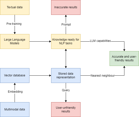
Figure 1: An ideal workflow for combining vector databases and large language models.

At first, the large language model is pre-trained using textual data, which stores knowledge that can be prepared for use in natural language processing tasks. The multimodal data is embedded and stored in a vector database to obtain vector representations. Next, when the user inputs a serialized textual question, the LLM is responsible for providing NLP capabilities, while the algorithms in the vector database are responsible for finding approximate nearest neighbors.

Combining the two gives more desirable results than using only LLM and the vector database. If only LLM is used, the results obtained may not be accurate enough, while if only vector databases are used, the results obtained may not be user-friendly.

V-B Vector Database for LLM

V-B1 Data

By learning from massive amounts of pre-training textual data, LLMs can acquire various emerging capabilties, which are not present in smaller models but are present in larger models, e.g., in-context learning, chain-of-thought, and instruction following [36], [37].

Data plays a crucial role in LLM’s emerging ability, which in turn can unfold at three points:

Data scale. This is the amount of data that is used to train the LLMs. According to [38], LLMs can improve their capabilities predictably with increasing data scale, even without targeted innovation. The larger the data scale, the more diverse and representative the data is, which can help the LLMs learn more patterns and relationships in natural language. LLMs can improve their capabilities predictably with increasing data scale, even without targeted innovation. However, data scale also comes with challenges, such as computational cost, environmental impact, and ethical issues.

Data quality. This is the accuracy, completeness, consistency, and relevance of the data that is used to train the LLMs. The higher the data quality, the more reliable and robust the LLMs are [39], which can help them avoid errors and biases. LLMs can benefit from data quality improvement techniques, such as data filtering, cleaning, augmentation, and balancing. However, data quality also requires careful evaluation and validation, which can be difficult and subjective.

Data diversity. This is the variety and richness of the data that is used to train the LLMs. The more diverse the data, the more inclusive and generalizable the LLMs are, which can help them handle different languages, domains, tasks, and users. LLMs can achieve better performance and robustness by using diverse data sources, such as web text, books, news articles, social media posts, and more. However, data diversity also poses challenges, such as data alignment, integration, and protection.

As for vector database, the traditional techniques of database such as cleaning, de-duplication and alignment can help LLM to obtain high-quality and large-scale data, and the storage in vector form is also suitable for diverse data.

V-B2 Model

In addition to the data, LLM has benefited from growth in model size. The large number of parameters creates challenges for model training, and storage. Vector databases can help LLM reduce costs and increase efficiency in this regard.

Distributed training. DBMS can help model storage in the context of model segmentation and integration. Vector databases can enable distributed training of LLM by allowing multiple workers to access and update the same vector data in parallel [40], [41]. This can speed up the training process and reduce the communication overhead among workers.

Model compression. The purpose of this is to reduce the complexity of the model and the number of parameters, reduce model storage and computational resources, and improve the efficiency of model computing. The methods used are typically pruning, quantization, grouped convolution, knowledge distillation, neural network compression, low-rank decomposition, and so on. Vector databases can help compress LLM by storing only the most important or representative vectors of the model, instead of the entire model parameters. This can reduce the storage space and memory usage of LLM, as well as the inference latency.

Vector storage. Vector databases can optimize the storage of vector data by using specialized data structures, such as inverted indexes, trees, graphs, or hashing. This can improve the performance and scalability of LLM applications that rely on vector operations, such as semantic search, recommendation, or question answering.

V-B3 Retrieval

Users can use a large language model to generate some text based on a query or a prompt, however, the output may not be diversiform, consistent, or factual. Vector databases can ameliorate these problems on a case-by-case basis, improving the user experience.

Cross-modal support. Vector databases can support cross-modal search, which is the ability to search across different types of data, such as text, images, audio, or video. For example, an LLM can use a vector database to find images that are relevant to a text query, or vice versa. This can enhance the user experience and satisfaction by providing more diverse and rich results.

Real-time knowledge. Vector databases can enable real-time knowledge search, which is the ability to search for the most up-to-date and accurate information from various sources. For example, an LLM can use a vector database to find the latest news, facts, or opinions about a topic or event. This can improve the user’s awareness and understanding by providing more timely and reliable results.

Less hallucination. Vector databases can help reduce hallucination, which is the tendency of LLM to generate false or misleading statements. For example, an LLM can use a vector database to verify or correct the data that it generates or uses for search. This can increase the user’s trust and confidence by providing more accurate and consistent results.

V-C Potential Applications for Vector Database on LLM

Vector databases and LLMs can work together to enhance each other’s capabilities and create more intelligent and interactive systems. Here are some potential applications for vector databases on LLMs:

V-C1 Long-term memory

Vector Databases can provide LLMs with long-term memory by storing relevant documents or information in vector form. When a user gives a prompt to an LLM, the Vector Database can quickly retrieve the most similar or related vectors from its index and update the context for the LLM. This way, the LLM can generate more customized and informed responses based on the user’s query and the Vector Database’s content.

V-C2 Semantic search

Vector Databases can enable semantic search for LLMs by allowing users to search for texts based on their meaning rather than keywords. For example, a user can ask an LLM a natural language question and the Vector Database can return the most relevant documents or passages that answer the question. The LLM can then summarize or paraphrase the answer for the user in natural language.

V-C3 Recommendation systems

Vector Databases can power recommendation systems for LLMs by finding similar or complementary items based on their vector representations. For example, a user can ask an LLM for a movie recommendation and the Vector Database can suggest movies that have similar plots, genres, actors, or ratings to the user’s preferences. The LLM can then explain why the movies are recommended and provide additional information or reviews.

V-D Potential Applications for LLM on Vector Database

LLMs on vector databases are also very interesting and promising. Here are some potential applications for LLMs on vector databases:

V-D1 Text generation

LLMs can generate natural language texts based on vector inputs from Vector Databases. For example, a user can provide a vector that represents a topic, a sentiment, a style, or a genre, and the LLM can generate a text that matches the vector. This can be useful for creating content such as articles, stories, poems, reviews, captions, summaries, etc. One corresponding study is [42].

V-D2 Text augmentation

LLMs can augment existing texts with additional information or details from Vector Databases. For example, a user can provide a text that is incomplete, vague, or boring, and the LLM can enrich it with relevant facts, examples, or expressions from Vector Databases. This can be useful for improving the quality and diversity of texts such as essays, reports, emails, blogs, etc. One corresponding study is [43].

V-D3 Text transformation

LLMs can transform texts from one form to another using VDBs. For example, a user can provide a text that is written in one language, domain, or format, and the LLM can convert it to another language, domain, or format using VDBs. This can be useful for tasks such as translation, paraphrasing, simplification, summarization, etc. One corresponding study is [44].

V-E Retrieval-Based LLM

V-E1 Definition

Retrieval-based LLM is a language model which retrieves from an external datastore (at least during inference time) [46].

V-E2 Strength

Retrieval-based LLM is a high-level synergy of LLMs and databases, which has several advantages over LLM only.

Memorize long-tail knowledge. Retrieval-based LLM can access external knowledge sources that contain more specific and diverse information than the pre-trained LLM parameters. This allows retrieval-based LLM to answer in-domain queries that cannot be answered by LLM only.

Easily updated. Retrieval-based LLM can dynamically retrieve the most relevant and up-to-date documents from the data sources according to the user input. This avoids the need to fine-tune the LLM on a fixed dataset, which can be costly and time-consuming.

Better for interpreting and verifying. Retrieval-based LLM can generate texts that cite their sources of information, which allows the user to validate the information and potentially change or update the underlying information based on requirements. Retrieval-based LLM can also use fact-checking modules to reduce the risk of hallucinations and errors.

Improved privacy guarantees. Retrieval-based LLM can protect the user’s privacy by using encryption and anonymization techniques to query the data sources. This prevents the data sources from collecting or leaking the user’s personal information or preferences [45]. Retrieval-based LLM can also use differential privacy methods to add noise to the retrieved documents or the generated texts, which can further enhance the privacy protection [47].

Reduce time and money cost. Retrieval-based LLM can save time and money for the user by reducing the computational and storage resources required for running the LLM. This is because retrieval-based LLM can leverage the existing data sources as external memory, rather than storing all the information in the LLM parameters. Retrieval-based LLM can also use caching and indexing techniques to speed up the document retrieval and passage extraction processes.

V-E3 Inference

Multiple parts of the data flow are involved in the inference session.

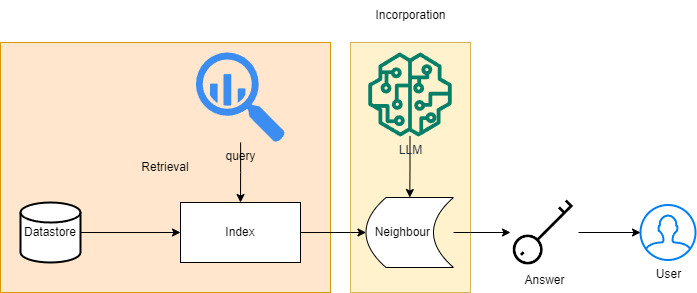
Figure 2: A retrieval-based LLM inference dataflow.

Datastore. The data store can be very diverse, it can have only one modality, such as a raw text corpus, or a vector database that integrates data of different modalities, and its treatment of the data determines the specific algorithms for subsequent retrieval. In the case of raw text corpus, which are generally at least a billion to trillion tokens, the dataset itself is unlabeled and unstructured, and can be used as a original knowledge base.

Index. When the user enters a query, it can be taken as the input for retrieval, followed by using a specific algorithm to find a small subset of the datastore that is closest to the query, in the case of vector databases the specific algorithms are the NNS and ANNS algorithms mentioned earlier.

V-F Synergized Example

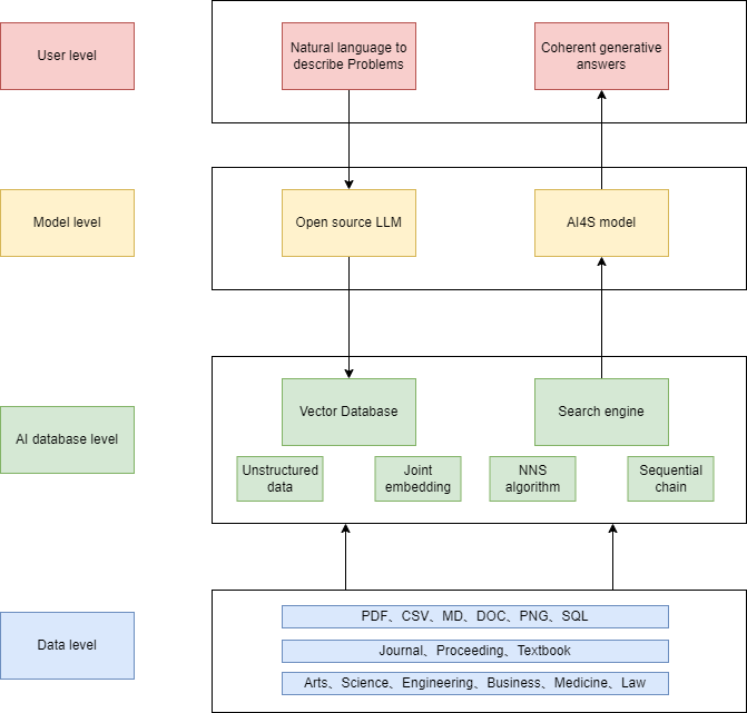
Figure 3: A complex application of vector database + LLM for scientific research.

For a workflow that incorporates a large language model and a vector database, it can be understood by splitting it into four levels: the user level, the model level, the AI database level, and the data level, respectively.

For a user who has never been exposed to large language modeling, it is possible to enter natural language to describe their problem. For a user who is proficient in large language modeling, a well-designed prompt can be entered.

The LLM next processes the problem to extract the keywords in it, or in the case of open source LLMs, the corresponding vector embeddings can be obtained directly.

The vector database stores unstructured data and their joint embeddings. The next step is to go to the vector database to find similar nearest neighbors. The ones obtained from the sequences in the big language model are compared with the vector encodings in the vector database, by means of the NNS or ANNS algorithms. And different results are derived through a predefined serialization chain, which plays the role of a search engine.

If it is not a generalized question, the results derived need to be further put into the domain model, for example, imagine we are seeking an intelligent scientific assistant, which can be put into the model of AI4S to get professional results. Eventually it can be placed again into the LLM to get coherent generated results.

For the data layer located at the bottom, one can choose from a variety of file formats such as PDF, CSV, MD, DOC, PNG, SQL, etc., and its sources can be journals, conferences, textbooks, and so on. Corresponding disciplines can be art, science, engineering, business, medicine, law, and etc.

VI Conclusion

In this paper, we provide a comprehensive and up-to-date literature review on vector databases. One of our main objective is to reorganize and introduce most of the research so far in a comparative perspective. In a first step, we discuss the storage in detail. We then thoroughly review NNS and ANNS approaches, and then discuss the challenges. Last but not least, we discuss the future about vector database with LLMs.

References

- [1] J. L. Bentley, “Multidimensional binary search trees used for associative searching,” Communications of the ACM, vol. 18, no. 9, p. 509–517, 1975.
- [2] B. Ghojogh, S. Sharifian, and H. Mohammadzade, “Tree-based optimization: A meta-algorithm for metaheuristic optimization,” 2018.
- [3] S. M. Omohundro, Five balltree construction algorithms. Berkeley: International Computer Science Institute, 1989.
- [4] T. Liu, A. W. Moore, A. Gray, and K. Yang, “New algorithms for efficient high-dimensional nonparametric classification,” Journal of machine learning research, vol. 7, no. 6, 2006.
- [5] S. Kumar and S. Kumar, “Ball*-tree: efficient spatial indexing for constrained nearest-neighbor search in metric spaces,‘’ arXiv preprint arXiv:1511.00628, 2015.
- [6] A. Guttman, “R-trees: a dynamic index structure for spatial searching,” in Proceedings of the 1984 ACM SIGMOD international conference on Management of data, p. 47–57, 1984.
- [7] P. Ciaccia, M. Patella, and P. Zezula, “M-tree: An efficient access method for similarity search in metric spaces,” in Vldb, vol. 97, p. 426–435, 1997.
- [8] D. Cai, “A revisit of hashing algorithms for approximate nearest neighbor search,‘’ arXiv preprint arXiv:1612.07545, 2019.
- [9] M. Datar, N. Immorlica, P. Indyk, and V. S. Mirrokni, “Locality-sensitive hashing scheme based on p-stable distributions,” in Proceedings of the twentieth annual symposium on Computational geometry, p. 253–262, 2004.
- [10] O. Jafari, P. Maurya, P. Nagarkar, K. M. Islam, and C. Crushev, “A survey on locality sensitive hashing algorithms and their applications,” 2021.
- [11] A. Andoni, P. Indyk, et al., “Locality sensitive hashing (lsh) home page.” ^1^, 2023. Accessed: 2023-10-18.
- [12] K. Bob, D. Teschner, T. Kemmer, D. Gomez-Zepeda, S. Tenzer, B. Schmidt, and A. Hildebrandt, “Locality-sensitive hashing enables efficient and scalable signal classification in high-throughput mass spectrometry raw data,” BMC Bioinformatics, vol. 23, no. 1, p. 287, 2022.
- [13] A. Andoni and P. Indyk, “Near-optimal hashing algorithms for approximate nearest neighbor in high dimensions,‘’ in 2006 47th Annual IEEE Symposium on Foundations of Computer Science (FOCS’06). IEEE, 2006, pp. 459–468.
- [14] A. Andoni, P. Indyk, T. Laarhoven, I. Peebles, and L. Schmidt, “Beyond locality-sensitive hashing,‘’ arXiv preprint arXiv:1306.1547, 2013.
- [15] Y.-C. Chen, T.-Y. Chen, Y.-Y. Lin, C.-S. Chen, and Y.-P. Hung, “Optimal data-dependent hashing for approximate near neighbors,‘’ arXiv preprint arXiv:1501.01062, 2015.
- [16] Y. Weiss, A. Torralba, and R. Fergus, “Spectral hashing,” Advances in neural information processing systems, vol. 21, 2008.
- [17] H. Liu, R. Wang, S. Shan, and X. Chen, “Deep supervised hashing for fast image retrieval,” in Proceedings of the IEEE conference on computer vision and pattern recognition, p. 2064–2072, 2016.
- [18] J.-H. Lee and J.-H. Kim, “Deep hashing using proxy loss on remote sensing image retrieval,‘’ Remote Sensing, vol. 13, no. 15, p. 2924, Jul. 2021.
- [19] X. Luo, H. Wang, D. Wu, C. Chen, M. Deng, J. Huang, and X.-S. Hua, “A survey on deep hashing methods,” 2022.
- [20] B. E and S. AB., “Annoy (approximate nearest neighbors oh yeah).” [DB/OL]. (2015) [2023-10-17]. 3, 2015.
- [21] B. J. S and L. D. G., “Shape indexing using approximate nearest-neighbour search in high-dimensional spaces,” in Proceedings of IEEE computer society conference on computer vision and pattern recognition, pp. 1000–1006, 1997.
- [22] H. Liu, M. Deng, and C. Xiao, “An improved best bin first algorithm for fast image registration,‘’ in Proceedings of 2011 International Conference on Electronic & Mechanical Engineering and Information Technology, vol. 1, 2011, pp. 355–358.
- [23] T. P, T. P, and S. M., “K-means tree: an optimal clustering tree for unsupervised learning,” The Journal of Supercomputing, vol. 77, pp. 5239–5266, 2021.
- [24] P. A, M. Y, L. A, and K. A., “Approximate nearest neighbor search small world approach,” in International Conference on Information and Communication Technologies & Applications, 2011.
- [25] M. Y, P. A, L. A, and K. A., “Scalable distributed algorithm for approximate nearest neighbor search problem in high dimensional general metric spaces,” in Similarity Search and Applications: 5th International Conference, SISAP 2012, Toronto, ON, Canada, August 9-10, 2012. Proceedings 5, pp. 132–147, 2012.
- [26] M. Y, P. A, L. A, and K. A., “Approximate nearest neighbor algorithm based on navigable small world graphs,” Information Systems, vol. 45, pp. 61–68, 2014.
- [27] Y. A. Malkov and D. A. Yashunin, “Efficient and robust approximate nearest neighbor search using hierarchical navigable small world graphs,” IEEE transactions on pattern analysis and machine intelligence, vol. 42, no. 4, p. 824–836, 2018.
- [28] Y. Wang, Z. Pan, and R. Li, “A new cell-level search based non-exhaustive approximate nearest neighbor (ann) search algorithm in the framework of product quantization,” IEEE Access, vol. 7, pp. 37059–37070, 2019.
- [29] H. Jegou, M. Douze, and C. Schmid, “Product quantization for nearest neighbor search,” IEEE transactions on pattern analysis and machine intelligence, vol. 33, no. 1, p. 117–128, 2010.
- [30] T. Ge, K. He, Q. Ke, and J. Sun, “Optimized product quantization,” IEEE transactions on pattern analysis and machine intelligence, vol. 36, no. 4, p. 744–755, 2013.
- [31] L. Li and Q. Hu, “Optimized high order product quantization for approximate nearest neighbors search,” Frontiers of Computer Science, vol. 14, no. 2, pp. 259–272, 2020.
- [32] D. Xu, I. W. Tsang, Y. Zhang, and J. Yang, “Online product quantization,” IEEE Transactions on Knowledge and Data Engineering, vol. 30, no. 11, p. 2185–2198, 2018.
- [33] W. X. Zhao et al., “A survey of large language models,‘’ arXiv preprint arXiv:2303.18223, 2023.
- [34] M. Shanahan, “Talking about large language models,” 2023.
- [35] OpenAI, “GPT-4 technical report,‘’ arXiv preprint arXiv:2303.08774, 2023.
- [36] J. Wei, Y. Tay, R. Bommasani, C. Raffel, B. Zoph, S. Borgeaud, D. Yogatama, M. Bosma, D. Zhou, D. Metzler, E. H. Chi, T. Hashimoto, O. Vinyals, P. Liang, J. Dean, and W. Fedus, “Emergent abilities of large language models,” 2022.
- [37] X. Yang, “The collision of databases and big language models - recent reflections,‘’ China Computer Federation, Tech. Rep., Jul. 2023.
- [38] S. R. Bowman, “Eight things to know about large language models,‘’ arXiv preprint arXiv:2304.00612, 2023.
- [39] A. Mallen et al., “When not to trust language models: Investigating effectiveness of parametric and non-parametric memories,‘’ arXiv preprint arXiv:2212.10511, 2023.
- [40] X. Nie et al., “FlexMoE: Scaling large-scale sparse pre-trained model training via dynamic device placement,‘’ Proceedings of the ACM on Management of Data, vol. 1, no. 1, pp. 1–19, May 2023.
- [41] X. Nie et al., “HetuMoE: An efficient trillion-scale mixture-of-expert distributed training system,‘’ arXiv preprint arXiv:2203.14685, 2022.
- [42] R. Tang, X. Han, X. Jiang, and X. Hu, “Does synthetic data generation of LLMs help clinical text mining¿’ arXiv preprint arXiv:2303.04360, 2023.
- [43] C. Whitehouse, M. Choudhury, and A. Fikri Aji, “LLM-powered data augmentation for enhanced crosslingual performance,‘’ arXiv preprint arXiv:2305.14288, 2023.
- [44] S. Chang and E. Fosler-Lussier, “How to prompt LLMs for text-to-SQL: A study in zero-shot, single-domain, and cross-domain settings,‘’ arXiv preprint arXiv:2305.11853, 2023.
- [45] J. Liu et al., “RETA-LLM: A retrieval-augmented large language model toolkit,‘’ arXiv preprint arXiv:2306.05212, 2023.
- [46] A. Asai, S. Min, Z. Zhong, and D. Chen, “ACL 2023 tutorial: Retrieval-based language models and applications,‘’ ACL 2023, 2023.
- [47] Y. Huang et al., “Privacy implications of retrieval-based language models,‘’ arXiv preprint arXiv:2305.14888, 2023.