Detection of 12426 SB2 candidates in the LAMOST-MRS, using a binary spectral model.

Abstract

We use an updated method for the detection of double-lined spectroscopic binaries (SB2) using $V\sin{i}$ values from spectral fits. The method is applied to all spectra from LAMOST MRS. Using this method, we detect 12426 SB2 candidates, where 4321 are already known and 8105 are new discoveries. We check their spectra manually to minimise possible false positives. We also detect several cases of contamination of the spectra by solar light. Additionally, for candidates with multiple observations we compute mass ratios with systemic velocities and determine Keplerian orbits. We present an updated catalogue of all SB2 candidates together with additional information for some of them in separate data tables.

1 Introduction

Kovalev et al. (2022b) presented a new method for detection of the double-lined spectroscopic binaries (SB2s) in LAMOST (Large Sky Area Multi-Object fiber Spectroscopic Telescope, also known as Guoshoujing telescope) Medium Resolution Survey (MRS). It is based on a clear correlation between the radial velocity separation ($\hbox{|$\Delta$ RV|}=|{\rm RV}_{1}-{\rm RV}_{2}|$) estimated by the binary model and the value of the projected rotational velocity $V\sin{i}_{0}$, derived by the single-star model for SB2 systems. It was proven that this method is able to identify SB2s even when the standard analysis of cross-correlation functions (CCF) fails. Two other studies, Kovalev et al. (2022a); Kovalev et al. (2023b), presented detailed analyses of the two SB2 systems using multiple spectroscopic observations simultaneously and proved that it is reliable. A recent study, Kovalev et al. (2023c) explored the problem of possible contamination of LAMOST-MRS spectra by the solar light reflected by the nearby objects and found out, that some SB2 candidates can be result of such contamination.

In this paper we continue the analysis of the LAMOST MRS using a binary spectral model. The methods from Kovalev et al. (2022b) are updated and applied to all available spectra. Thus we significantly expand our catalogue, which now has six times more SB2 candidates, and also present more detailed results for many of them.

The paper is organised as follows: in Sections 2 and 3, we describe the observations and methods. Section 4 presents our results. In Section 5 we discuss the results. In Section 6 we summarise the paper and draw conclusions.

2 Observations

LAMOST is a 4-metre quasi-meridian reflective Schmidt telescope with 4000 fibers installed on its $5\degr$ FoV focal plane. These configurations allow it to observe spectra for at most 4000 celestial objects simultaneously (Cui et al. (2012); Zhao et al. (2012)). In comparison with Kovalev et al. (2022b) which was restricted only to time-domain spectra, in this paper we downloaded all available spectra from www.lamost.org, including non-time-domain (NT) spectra. We use the spectra taken at a resolving power of $R=\lambda/\Delta\lambda\sim 7\,500$. Each spectrum is divided on two arms: blue from 4950 Å to 5350 Å and red from 6300 Å to 6800 Å. We convert the heliocentric wavelength scale in the observed spectra from vacuum to air using PyAstronomy (Czesla et al., 2019). Observations are carried out in MJD=58407.6-59736.8 days, spanning an interval of 1329 days. We selected only spectra stacked within a single night and apply a cut on the signal-to-noise (S/N). In total we have $1\,805\,736$ spectra from $840\,826$ targets, where the $\hbox{S/N}\geq 20$ ${\rm pix}^{-1}$ in any of spectral arms. The majority of the spectra (one half) sample the S/N in the range of 40-250 ${\rm pix}^{-1}$. The number of exposures varies from 1 to 40 per target, as noisy exposures were not selected for many targets.

3 Methods

3.1 Spectroscopic analysis

We use the same spectroscopic models and method as Kovalev et al. (2022a) to analyse individual LAMOST-MRS spectra, see brief description below. The normalised binary model spectrum is generated as a sum of the two Doppler-shifted normalised single-star spectral models ${f}_{\lambda,i}$, scaled according to the difference in luminosity, which is a function of the ${T_{\rm eff}}$ and stellar size. We assume both components to be spherical.

The binary model spectrum is later multiplied by the normalisation function, which is a linear combination of the first four Chebyshev polynomials (similar to Kovalev et al., 2019), defined separately for the blue and red arms of the spectrum. The resulting spectrum is compared with the observed one using scipy.optimise.curve_fit function, which provides the optimal spectral parameters and radial velocities (RV) for each component plus the stellar radii ratio $k_{R}={R_{1}}/{R_{2}}$ and two sets of four coefficients of the Chebyshev polynomials. We keep the metallicity equal for both components. In total we have 18 free parameters for a binary fit. We estimate the goodness of the fit parameter by reduced $\chi^{2}$.

Additionally, every spectrum is analysed by a single star model, which is identical to a binary model when both components have all equal parameters, so we fit only for 13 free parameters. Using this single star solution we compute the difference in reduced $\chi^{2}$ between two solutions and the improvement factor ($f_{\rm imp}$), computed using Equation 1 similar to El-Badry et al. (2018). This improvement factor estimates the absolute value difference between two fits and weights it by the difference between the two solutions.

$$f_{{\rm imp}}=\frac{\sum_{\lambda=\lambda_{min}}^{\lambda=\lambda_{max}}\left[\left(\left|{f}_{\lambda,{\rm single}}-{f}_{\lambda}\right|-\left|{f}_{\lambda,{\rm binary}}-{f}_{\lambda}\right|\right)/{\sigma}_{\lambda}\right]}{\sum_{\lambda=\lambda_{min}}^{\lambda=\lambda_{max}}\left[\left|{f}_{\lambda,{\rm single}}-{f}_{\lambda,{\rm binary}}\right|/{\sigma}_{\lambda}\right]},$$ (1)

where ${f}_{\lambda}$ and ${\sigma}_{\lambda}$ are the observed flux and corresponding uncertainty, ${f}_{\lambda,{\rm single}}$ and ${f}_{\lambda,{\rm binary}}$ are the best-fit single-star and binary model spectra, and the sum is over all wavelength pixels.

3.2 Selection of SB2 candidates

Here we use the same logic as Kovalev et al. (2022b) for selection: we separate single stars from binary solutions. If we try to fit the double-lined spectrum with $\hbox{|$\Delta$ RV|}>0$ using a single star model there are three possible outcomes:

1. none of the spectral components are well constrained, but $V\sin{i}_{0}$ proportional to |$\Delta$ RV| is large enough that the broadened model covers both of them;

2. only one spectral component (usually the primary) is well fitted, while the other is completely ignored by the single-star spectral model;

3. the spectrum is poorly fitted because the synthetic model is unable to reproduce a real spectrum due to missing physics (usually emission lines, molecular bands etc.) or data processing artifacts.

For all these cases binary model fits the spectrum much better and $f_{\rm imp}$ is large. However case 1 is most useful to select SB2s. Even small |$\Delta$ RV|, which is insufficient to split spectral lines due to finite spectrograph’s resolution, will cause a change to the spectral lines: they will become broader and the fitted value of $V\sin{i}_{0}$ will increase in comparison with the value from the spectrum of that binary taken when $\hbox{|$\Delta$ RV|}=0$. Case 2 can be excluded by requiring ${\rm RV}_{1}$ to differ from ${\rm RV}_{0}$, as for such a case value $V\sin{i}_{0}$ is useless for SB2 identification. However, it can be used if the binary model had a good fit, so we put some thresholds on $f_{\rm imp}$ and the ratio of $\chi_{\rm single}/\chi_{\rm binary}$. Multiple epochs can also allow us to find an SB2 candidate by $V\sin{i}_{0}$ variation, which it is proportional to |$\Delta$ RV|, although such a variation can be caused by a real change of $V\sin{i}$.

Now we need to separate out the single stars. When a single star spectrum with $V\sin{i}_{0}$ is fitted by a binary model there are three possible outcomes:

1. the spectrum is well fitted by a twin binary model, consisting of two components similar to the real star with small $\hbox{|$\Delta$ RV|}\sim 0$, therefore $V\sin{i}_{1,2}\sim V\sin{i}_{0}$ and $V\sin{i}_{1}+V\sin{i}_{2}\sim 2V\sin{i}_{0}$;

2. the spectrum is well fitted by the primary component, which is almost identical to the real star ($V\sin{i}_{1}\sim V\sin{i}_{0}$), and a small or negligible contribution from the secondary component, which can have any value $V\sin{i}_{2}$, although usually it is quite large, so the secondary spectrum looks completely “flat";

3. the spectrum is poorly fitted as the synthetic model is unable to reproduce the real spectrum. In this case, the binary model is desperately trying to compensate for the missing spectral information by combining two spectral components, usually with significant improvement relative to best single star model.

For cases 1 and 2, $f_{\rm imp}$ is usually small, but for case 3 it can be quite large. Thus we can select SB2 candidates with $\hbox{|$\Delta$ RV|}>0$ by selecting the spectra with $V\sin{i}_{1}+V\sin{i}_{2}+V\sin{i}_{\rm min}<V\sin{i}_{0}$ and ${\rm RV}_{1}\neq{\rm RV}_{0}$, while “bad fits" from case 3 can be excluded using a cut on $f_{\rm imp}$. $V\sin{i}_{\rm min}$ takes into account the possible uncertainties in the $V\sin{i}$ measurements. However we should note that these criteria will not select spectra of fast rotators, as in this case $V\sin{i}_{1}+V\sin{i}_{2}>V\sin{i}_{0}$ for small $\hbox{|$\Delta$ RV|}>0$. They can be selected only for a significant |$\Delta$ RV|. This is our standard selection. More SB2 candidates from case 2 with the single-star model fitting only a primary are selected using ${\rm RV}_{1}\sim{\rm RV}_{0}$ and cuts on $f_{\rm imp}$ and $\chi_{\rm single}/\chi_{\rm binary}$, which can be found empirically. We call such selection “selected by primary". An interesting system J065032.45+231030.2 mentioned, but not selected in Kovalev et al. (2022b), is selected by these criteria.

3.3 Updates relative to previous version

In this section we summarize all updates applied to the methods in this paper, in comparison with Kovalev et al. (2022b):

1. we switch from neural network based spectral model of the single star to simple linear interpolation, see Appendix A,

2. for the binary spectral model we directly use the ratio of stellar radii $k_{R}$ as a fitting parameter, instead of the mass ratio which was later combined with the difference of the surface gravities $\log{\rm(g)}$ to get the ratio of stellar radii.

3. we introduce a new “selection by primary" for SB2 candidates, where the single-star spectral model ignores secondary component.

4. we manually checked all selected SB2 candidates to minimise number of false-positives detections.

4 Results

Figure 1: Values of $V\sin{i}$ for the observed dataset (top panel) and selected spectra (bottom panel). Solid lines show the functions $V\sin{i}_{1}+V\sin{i}_{2}=V\sin{i}_{0}$ (blue) and $V\sin{i}_{1}+V\sin{i}_{2}=2V\sin{i}_{0}$ (red). Selected stars confirmed via visual inspection are shown with black circles (standard selection) and pink circles (selected by primary).

4.1 Quality cuts

We carefully check the quality of the spectral fits through visual inspection of the plots. Our LAMOST-MRS dataset contains spectra from various targets and some of them can be poorly fitted by our spectral model (red super giants, very hot stars etc.). Therefore we introduce several quality cuts on the fitted parameters, see Table 1. These cuts keep $1\,497\,275$ spectra (83 per cent) from the original data set. Additionally we find $1367$ spectra, where the wavelength scale is clearly shifted between the blue and left arms, which is six times more than in Kovalev et al. (2022b).

Table 1: Quality cuts and selection criteria.

bad fits - any of the following cuts (293203 spectra):
$\chi^{2}_{\rm single}$ >12000
|$\Delta$ RV| >1320 $\,{\rm km}\,{\rm s}^{-1}$
|${\rm RV}_{0}$| >400 $\,{\rm km}\,{\rm s}^{-1}$
|$\log{k_{R}}$| >0.99
$k_{5000\AA}/(1+k_{5000\AA})$ >0.96
$\hbox{[Fe/H]}_{0}$<-0.77 and ${T_{\rm eff}}_{0}$>8600 K
$\hbox{[Fe/H]}_{1}$<-0.77 and ${T_{\rm eff}}_{1}$>8600 K
|$\hbox{[Fe/H]}_{0}$|>0.49 and $V\sin{i}_{0}$>289 $\,{\rm km}\,{\rm s}^{-1}$
|$\log{\rm(g)}_{0}-3$|>1.89 and $V\sin{i}_{0}$>289 $\,{\rm km}\,{\rm s}^{-1}$
|$\log{\rm(g)}_{0}-3$|>1.89 and ${{T_{\rm eff}}}_{0}$>8690 K
|$\log{\rm(g)}_{1}-3$|>1.89 and ${{T_{\rm eff}}}_{1}$>8690 K
Bad $\lambda$ calibration in 1367 spectra
standard SB2 selection (21962 spectra):
not in bad fits
$f_{\rm imp}$ >0.10
|${\rm RV}_{1}-{\rm RV}_{0}$| >10 $\,{\rm km}\,{\rm s}^{-1}$
$V\sin{i}_{1}+V\sin{i}_{2}$ +0.5< $V\sin{i}_{0}$
SB2 selection by primary (2613 spectra):
not in bad fits
$f_{\rm imp}$ >0.20
|${\rm RV}_{1}-{\rm RV}_{0}$| <=10 $\,{\rm km}\,{\rm s}^{-1}$
$\chi_{\rm single}/\chi_{\rm binary}>1.5$

4.2 Selected SB2 candidates

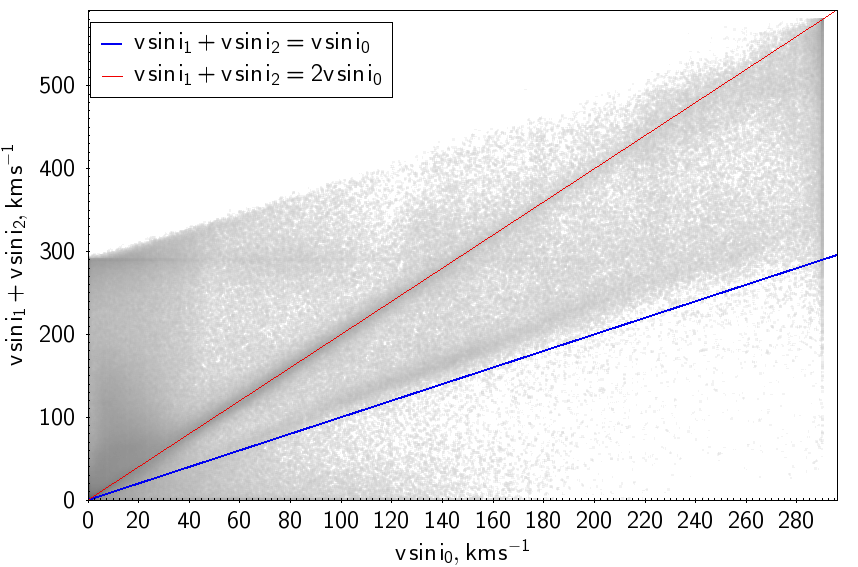
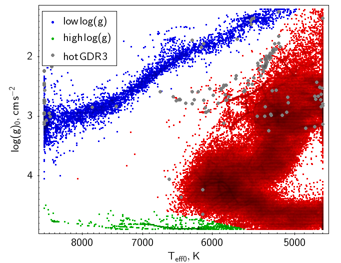
We show the plot with $V\sin{i}$ values, like in Kovalev et al. (2022b), in the top panel of Fig. 1. It is clearly seen that many datapoints follow the red line and a slightly broad region above the blue line, which are the places where single stars should be. We have overdensities at $V\sin{i}_{0}=290\,\,{\rm km}\,{\rm s}^{-1}$ and $V\sin{i}_{1}+V\sin{i}_{2}=290\,\,{\rm km}\,{\rm s}^{-1}$, where some value of $V\sin{i}$ is maximal. The first one is due to a restriction on extrapolation, while the second is formed by the stars where one of the components have maximal value of $V\sin{i}$ and usually shows no spectral lines. In comparison with Kovalev et al. (2022b) there is no gap at $V\sin{i}_{0}\sim 90\,\,{\rm km}\,{\rm s}^{-1}$. The gap was caused by a systematic problem in the fitting mechanism, which is gone as we replaced the neural network based spectrum generator by the simple linear interpolation. On the bottom panel we show selected SB2s candidates, confirmed by the manual inspection of the plots. We keep 19503 spectra in standard selection and 1839 in selected by primary subsets. In total we select 21342 spectra of 12426 stars.

4.3 Mass ratio measurements using the Wilson method.

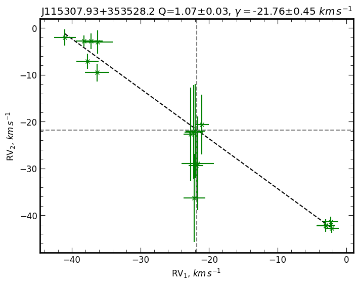
For SB2 candidates with several ($>3$) spectra and good ${\rm RV}_{1,2}$ measurements we can get dynamical mass ratios using the Wilson plot (Wilson, 1941; Kounkel et al., 2021). If two components in our binary system are gravitationally bound, their radial velocities should agree with the following equation (Wilson, 1941):

$${\rm RV_{1}}=\gamma_{\rm dyn}(1+Q_{\rm dyn})-Q_{\rm dyn}{\rm RV_{2}},$$ (2)

where $Q_{\rm dyn}={M_{1}}/{M_{2}}$ - mass ratio of binary components and $\gamma_{\rm dyn}$ - systemic velocity. Using this equation we can directly measure the systemic velocity and mass ratio by fitting the line, using orthogonal distance regression (ODR) method (Boggs & Rogers, 1990) which can handle uncertainty in both variables.

In Fig. 2 we show example of such fitting in the Wilson plot. Note that many datapoints with large errors are concentrated close to $\gamma$. Fortunately they did not affect final result as we have enough measurements near the extreme ${\rm RV}$ positions.

Figure 2: Wilson plot for J115307.93+353528.2 SB2 candidate. The mass ratio and systemic velocity from the ODR fit are shown in the title. The $\gamma$ is also shown by dashed vertical and horizontal lines.

We present the results for dynamical mass ratios and $\gamma$ in Table 3. Also we computed weighted the Pearson correlation coefficient for all datapoints to select good solutions that follow the straight line.

$$R_{w}=\frac{cov(x,y)}{\sqrt{cov(x,x)cov(y,y)}}$$ (3)

$$cov(x,y)=\sum\frac{w(x-\langle x\rangle)(y-\langle y\rangle)}{\sum w}$$ (4)

$$\langle x\rangle=\frac{\sum wx}{\sum w},w=\sigma^{-1}$$ (5)

Some values of mass ratios are very small and even negative (which have no physical meaning). Kounkel et al. (2021) also found such values using similar method. We suspect that such values are from spectroscopic triples or from chance alignment of spectroscopic binary with another star. We study three these objects in separate paper (Kovalev et al., 2023a).

4.4 Orbital solutions

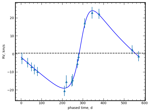
For stars with $N\geq 6$, good ${\rm RV}_{1}$ measurements, and $R_{w}<-0.95$, we use a Generalised Lomb-Scargle periodogram (GLS) by Zechmeister & Kürster (2009) to get orbits using circular and Keplerian solutions. We checked periods in the range $P=1,1000$ d on the regular grid of $e=0,0.8$ and $\omega=0,359^{\circ}$ with steps 0.01 and $1^{\circ}$ respectively. All parameters have errors provided by GLS, except for Keplerian orbits for ${\rm RV}$ time series with six measurements, which have infinite errors. For several solutions with $P=1000$ d we refined the solution using periods in the range $P=100,10000$ d. The example of the Keplerian orbit for J065032.45+231030.2 is shown on Figure 3.

Figure 3: Example of the Keplerian orbit for primary component of J065032.45+231030.2 derived using GLS.

Figure 4: Histogram for periods derived using GLS.

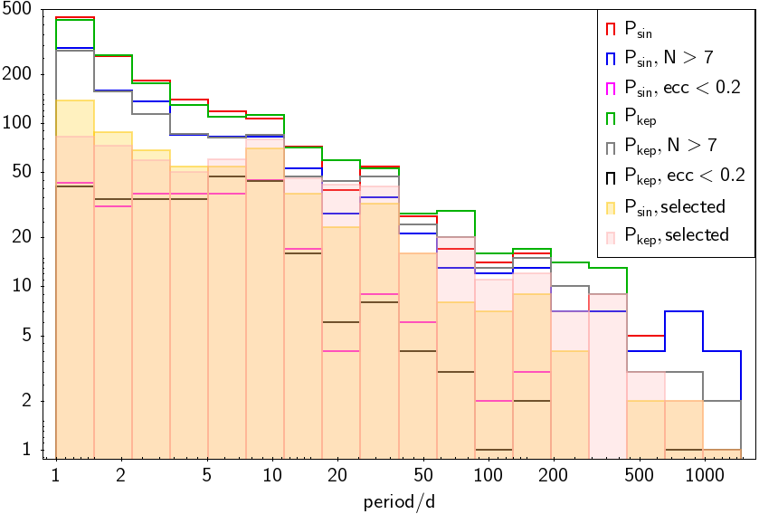
We show histograms for the periods computed with circular and Keplerian orbits in Figure 4. A significant fraction of the stars with $P<2$ d have large eccentricities ($e>0.2$) which is suspicious, as close binaries usually have circular orbits (Kounkel et al., 2021). This is likely due to the use of stacked spectra for ${\rm RV}$ determination with small temporal resolution. Thus we decided to check and discard many such suspicious solutions. After visual inspection of the results we selected 616 reliable solutions both circular and Keplerian, listed in Table 4. It is interesting that for J064726.39+223431.7 even using stacked spectra we were able to get a period $P=1.217842\pm 0.000012$ d which is very close to results from analysis of individual short exposures $P=1.217770\pm 0.000003$ d (Kovalev et al., 2023b). We think this is due to large semiamplitude ($K\sim 122~{}\,{\rm km}\,{\rm s}^{-1}$) of the orbit in this system.

5 Discussion

5.1 Comparison with other SB2 catalogues

We make cross matches with several available SB2 catalogues, and find more matches than Kovalev et al. (2022b), which is not surprising as we analysed significantly more targets. We find 863 matches with SIMBAD database (Wenger et al., 2000), labelled as SB*, seven matches with SB9 (Pourbaix et al., 2004), 141 matches with Traven et al. (2020), and 367 matches with Kounkel et al. (2021) catalogues. Cross matching with El-Badry et al. (2018) we find 24 stars listed in their SB2 table. Surprisingly, we find four matches (three new in comparison with Kovalev et al. (2022b)) with their single star table and one match with the SB1 table. We find no matches with either the SB3 table or the SB2 table with unseen third component. Among LAMOST-MRS based papers we find 1276 SB2 matches and 50 SB3 matches with Li et al. (2021), 292 matches with Wang et al. (2021), 1144 matches with Zhang et al. (2022) and 436 matches with Zheng et al. (2023). We find 594 matches with recent Gaia DR3 non-single stars orbits catalogue(Gaia Collaboration et al., 2022a), although only 236 and 231 are labelled as SB2 and SB1 respectively. By comparing with catalogue in Kovalev et al. (2022b) we confirm 2073 out of 2460 SB2 candidates, with rest unable to pass visual inspection of the plots.

In total our catalogue includes 12426 SB2 candidates, where 4321 are known and 8105 are new. Some of them are definitely spectroscopic triples or even quadruples, however the current selection method cannot distinguish them from SB2s. We note that some SB2 candidates can be chance alignments due to relatively large fiber diameter of the spectrograph (3″) or a result of contamination of the spectra by solar light, reflected by close objects (Kovalev et al., 2023c), see Section 5.2.

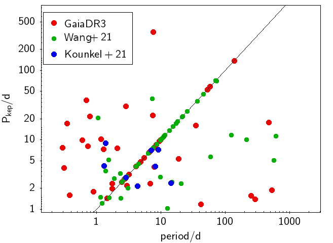
We compare our GLS periods with available periods from the literature in Figure 5. We found 44, 48 and 8 period values in Gaia Collaboration et al. (2022a),Wang et al. (2021) and Kounkel et al. (2021). Many values agree, but a significant fraction are very different, so we recommend to use our periods with care. Currently we use only the primary ${\rm RV}$ to determine the orbit, but we plan to use data for both components (similarly to Kounkel et al., 2021) in our future study.

Figure 5: Comparison of the Keplerian periods derived using GLS with literature values.

5.2 Contaminated spectra

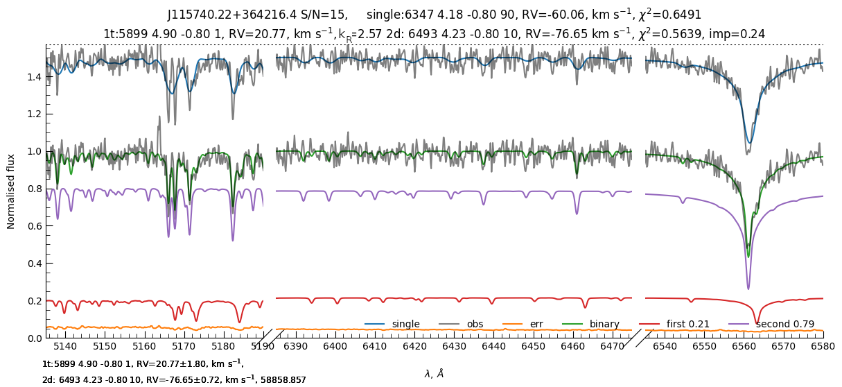
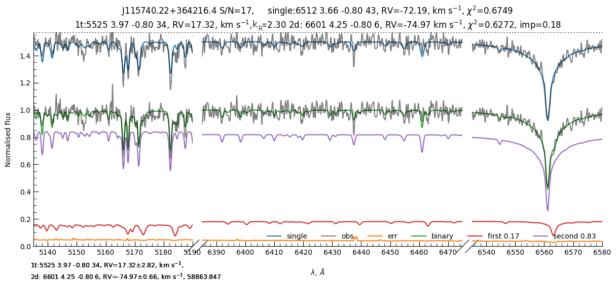
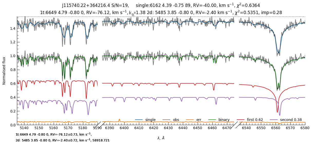
In Kovalev et al. (2022b) the spectrum of J055923.95+303104.2 taken at MJD=58531.535 d was indicated as a possible SB2 candidate, where a single star model fits only narrow lines of the secondary component. This narrow-lined component was absent in all other spectral observations, thus we proposed that this spectrum was taken during the partial eclipse. However there is another simple explanation: this is scattered light from the full Moon located at $\sim 29\degr$ from the field center, which can be seen as narrow-lined component with ${\rm RV}_{2}\sim-{\rm RV}_{\rm heliocentric}$.

We found several targets with similar contamination. See Figure 6 for J115740.22+364216.4. Three spectra taken at epochs MJD=$58858.857,\,58863.847,\,58918.721$ d have Moon’s phases $14.78,\,18.78,\,14.92$ d (out of 29.53 d) respectively. The ${\rm RV}_{\rm heliocentric}=-20.37,\,-18.96,\,2.98~{}\,{\rm km}\,{\rm s}^{-1}$ from the FITS file headers, taken with opposite sign, agree very well with ${\rm RV}_{2}=20.77\pm 1.80,\,17.32\pm 2.82,\,-2.40\pm 0.72~{}\,{\rm km}\,{\rm s}^{-1}$ derived by our binary model.

Figure 6: Examples of the spectra with possible contamination by the scattered Moon’s light. The fitting by the binary spectral model and single-star model are shown as green and blue (with offset 0.5) lines respectively. The observed spectrum and its error are shown as a gray and orange lines respectively. The primary (magenta line) and secondary (red line) components are labelled as "second" and "first" with contribution to total light at $\lambda=5000$ Å. The spectral parameters (${T_{\rm eff}},~{}\log{\rm(g)},~{}\hbox{[Fe/H]},~{}V\sin{i}$) from the single star model fit and the binary model fit are shown in the titles.

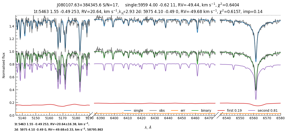
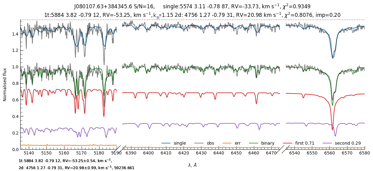
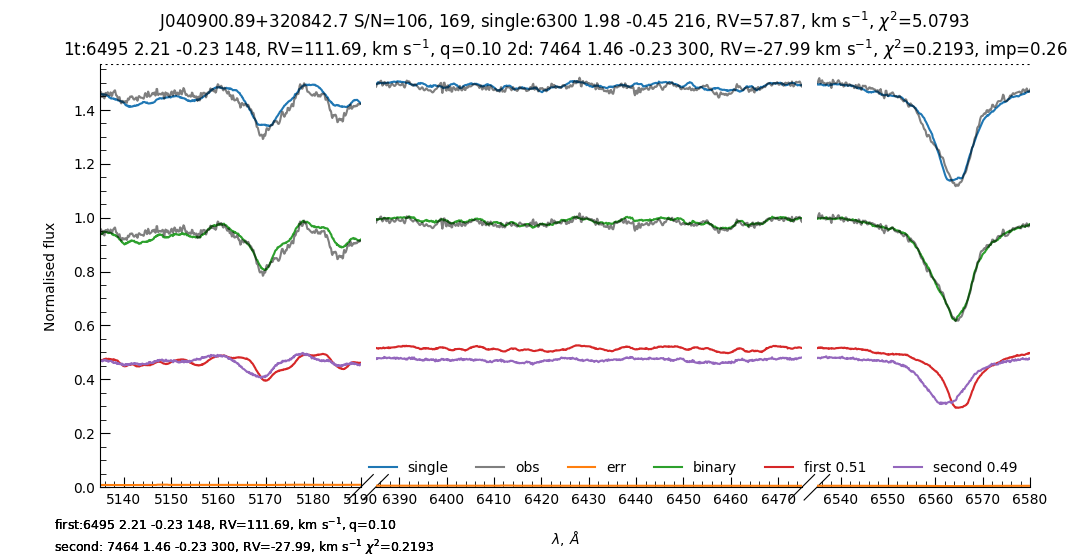
Another interesting target is J080107.63+384345.6 with $G=14.691$ mag. Only one ( observed at MJD=59236.661 d) of it’s spectra have been selected as SB2 candidate with significant $\Delta{\rm RV}\sim 73~{}\,{\rm km}\,{\rm s}^{-1}$ between components, while all other seven are well fitted by single-star model with ${\rm RV}\sim-50~{}\,{\rm km}\,{\rm s}^{-1}$, see Figure 7. The ODR fit provides very small $Q_{\rm dyn}~{}\sim 0.05$ which is very suspicious, so we suspected contamination by reflected solar light from artificial satellites. However it is unlikely as contaminant’s ${\rm RV}=20.98\pm 0.99~{}\,{\rm km}\,{\rm s}^{-1}$ is not consistent with ${\rm RV}_{\rm heliocentric}=3.96~{}\,{\rm km}\,{\rm s}^{-1}$. The Moon’s phase is also not full 9.62 d. We also checked for other solar-system bodies with Minor Planet Center checker, but found no objects brighter than $V=21$ mag close to our target at the moment of observation. Currently we don’t have clear explanation for this strange spectrum, although it can be a relatively long period, high eccentric binary, observed at the moment of periastron passage, so |$\Delta$ RV| was significant for detection.

Figure 7: Same as Fig.6 but for J080107.63+384345.6: the top panel shows the spectrum is well fit by the single-star model, and the spectrum in the bottom panel indicates an some unknown contamination.

5.3 Gaia DR3 data for LAMOST-MRS spectra

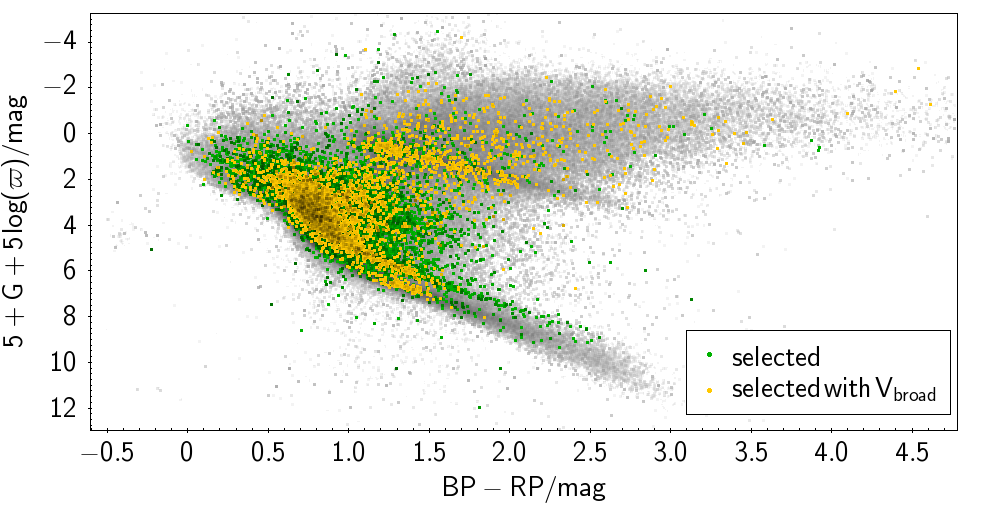
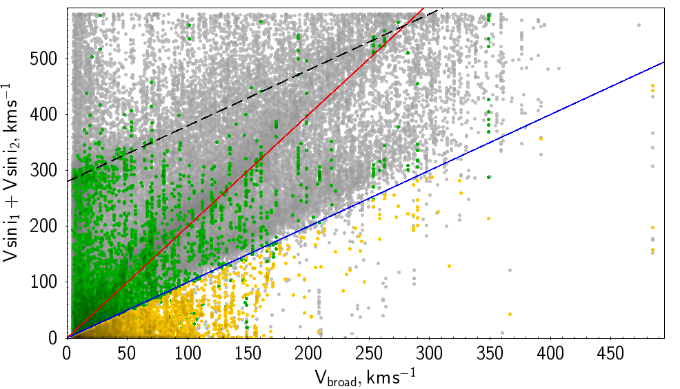
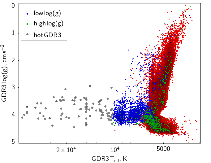
We check the recent Gaia DR3 (Gaia Collaboration et al., 2016, 2022b) and plot the Hertzsprung-Russell diagram for all matches with positive parallax in top panel of Fig 8. Selected SB2 candidates are shown with green triangles. Some of them are located at the main sequence of binaries with similar luminosity which is $\sim 0.75$ mag higher than main sequence. Gaia DR3 provides parameter $v_{\rm broad}$ as a measure of rotational broadening for a single stars, based on Gaia RVS spectra (Frémat et al., 2022). We use it instead of $V\sin{i}_{0}$ and reproduce bottom panel of Fig. 1 in the bottom panel of Fig. 8. Similarly to Fig. 1, not-selected stars slightly follow the red and blue lines. We have an overdensity at $v_{\rm broad}<10\,\,{\rm km}\,{\rm s}^{-1}$, and we have many hot stars in the region higher than the black dashed line $V\sin{i}_{1}+V\sin{i}_{2}=v_{\rm broad}+300$. In Fig. 1 this space was empty, because our fitting algorithm is unable fit ${T_{\rm eff}}>8800$ K, so it tries to increase $V\sin{i}_{0}$ in order to compensate for changes in the spectra. We apply the same selection as before using $v_{\rm broad}$ instead of $V\sin{i}_{0}$ and find 6116 spectra (3764 stars), where 3784 (1880 stars) of them were previously selected using $V\sin{i}_{0}$. We show them as green and yellow circles respectively. The remaining stars were probably observed by LAMOST-MRS at moments with $\hbox{|$\Delta$ RV|}\sim 0~{}\,{\rm km}\,{\rm s}^{-1}$. Unfortunately we can’t check this hypothesis, because epoch’s RVS spectra and RV measurements aren’t included in Gaia DR3.

Figure 8: Gaia DR3 Hertzsprung-Russell diagram for observed LAMOST-MRS dataset (top panel) and $V\sin{i}_{1}+V\sin{i}_{2}$ versus $v_{\rm broad}$ (bottom panel). SB2 candidates selected in Fig.1 are shown with green circles, SB2 candidates selected using $v_{\rm broad}$ are shown with yellow circles.

We compare our estimates for the subset of single stars with good fit spectra (selected using cuts in Table 1) and $\chi_{\rm single}<\chi_{\rm binary}$ with their matches in Gaia DR3 estimates in Figure 9. It is evident that the sequence of stars with $\log{\rm(g)}_{0}<3$ have $\log{\rm(g)}\sim 4$ in Gaia DR3 (shown as blue markers). In Kovalev et al. (2023b) spectroscopic $\log{\rm(g)}$ were also underestimated in comparison with values derived during the modelling of light curves, although the bias was much smaller. Thus we think that information in LAMOST-MRS spectra alone can not confidently constrain the surface gravity for stars with ${T_{\rm eff}}>6500$ K. Another group with high $\log{\rm(g)}_{0}>4.5$ dex and ${T_{\rm eff}}_{0}>5700$ K, shown as green circles, in Gaia DR3 have $\log{\rm(g)}$ in range from 0 to 4.6 dex. We checked their spectral plots and eventually almost all of them don’t have spectral data in red arm. Hot stars in Gaia DR3 with ${T_{\rm eff}}>10000$ K were mostly placed to the left of the red giants branch. Inspection of their plots found that many of them have no spectral features except strong emission in H$\alpha$. Other such stars were placed at the maximal value ${T_{\rm eff}}\sim 8790$ K or at the red giant branch. These red giants were confirmed by the visual inspection of the plots and probably were misclassified by Gaia DR3.

Figure 9: Comparison of the Kiel diagram for selected subset of the single stars (top panel) with corresponding Kiel diagram for their matches in Gaia DR3 (bottom panel).

The estimations of the spectral parameters can have significant biases. These parameters should be seen not as exact measurements, but more like set of parameters that represent best fit flexible template, similar to one used for RV determination using cross-correlation functions (see Gaia Collaboration et al. (2022b) that have published best template parameters for radial velocity spectrograph).

6 Conclusions

We have used an updated method for the detection of double-lined spectroscopic binaries (SB2) using $V\sin{i}$ values from spectral fits. The method is applied to all spectra from LAMOST-MRS. This method found 12426 (8105 new) SB2 candidates in the LAMOST-MRS. The updated method allows one to select many SB2 candidates, including ones with zero $\Delta{\rm RV}$ between components, if they have different spectra. We present a determination of the mass ratios and orbits for a subset of SB2 candidates with multiple observations. We also detect several cases where the spectra are contaminated by solar light, which can be identified by using our binary spectral model.

Data Availability

The data underlying this article will be shared on reasonable request to the corresponding author. LAMOST-MRS spectra are downloaded from www.lamost.org.

Appendix A Spectral model for LAMOST-MRS

The grid of synthetic spectra (6200 in total) is generated using the NLTE MPIA online-interface https://nlte.mpia.de (see Chapter 4 in Kovalev, 2019) on wavelength intervals 4870:5430 Å for the blue arm and 6200:6900 Å for the red arm with spectral resolution $R=7500$. We use a NLTE (non-local thermodynamic equilibrium) spectral synthesis for H, Mg I, Si I, Ca I, Ti I, Fe I and Fe II lines (see Chapter 4 in Kovalev, 2019, for references). The spectral parameters are randomly selected in a range of ${T_{\rm eff}}$=4600, 8800 K, $\log{\rm(g)}$=1.0, 4.99 (cgs units), $V\sin{i}$= 0, 300 $\,{\rm km}\,{\rm s}^{-1}$ and [Fe/H]=$-$0.9,$+$0.9 dex, microturbulence is fixed to $V_{\rm mic}=2~{}\,{\rm km}\,{\rm s}^{-1}$. We found that neural network (NN) generated spectrum used in Kovalev et al. (2022b) can contain small artefacts (usually smaller or comparable to the noise level) that disturb correct rotational profiles for a broad lines, which can lead to errors. Thus we replaced NN with a standard linear interpolation in four-dimensional space and used output of scipy.interpolate.LinearNDinterpolate as a single-star spectral model ${f}_{\lambda,{\rm single}}$. See Figure 10 with comparison of NN and linear interpolation results for one spectrum. It is clear that a linear interpolation provides smooth line profiles with “bell-like" shape for H$\alpha$, while line profile generated by NN has the wrong shape.

Figure 10: Same as Fig.6 but with results SB2 candidate of two fast rotators fitted with NN generated spectral model (top) and with linear interpolation of spectral models (bottom).

Appendix B Catalogue of SB2 candidates in LAMOST-MRS

Table 2 lists all 12426 SB2 candidates. We note that LAMOST designation can slightly vary between data releases, therefore we recommend to use Gaia DR3 source_id from Gaia Collaboration et al. (2022b).

Table 2: Catalogue of SB2 candidates in LAMOST-MRS. Full table is available as supplementary material.

LAMOST designation	Gaia DR3 source_id
J000000.18+320847.1	2873824744457023360
J000006.63+492648.6	393492950765727872
J000021.70+383903.8	2880989157927180800
..	..

Appendix C Data tables

In Tables 3,4 we present results for detailed analysis of SB2 candidates with multiple spectra.

Table 3: Dynamical mass ratios and systemic velocities. Full table is available as supplementary material.

Star	$\gamma_{\rm dyn}$, $\,{\rm km}\,{\rm s}^{-1}$	$Q_{\rm dyn}$	Gaia DR3 source_id
J000223.56+340644.8	$-38.84\pm 0.16$	$1.098\pm 0.006$	2875159070536814464
J000247.24+351645.5	$-15.36\pm 0.98$	$1.790\pm 0.057$	2876964296830796160
J000429.80+363651.3	$-16.51\pm 0.47$	$1.04\pm 0.02$	2877196774820732288
..	..	..	..

Table 4: Orbital parameters from GLS. Full table is available as supplementary material.

parameter	unit
NAME	JHHMMSS.SS+DDMMSS.S
$N_{\rm sp}$
$P_{\rm sin}$	d
$\sigma P_{\rm sin}$	d
$K_{\rm sin}$	$\,{\rm km}\,{\rm s}^{-1}$
$\sigma K_{\rm sin}$	$\,{\rm km}\,{\rm s}^{-1}$
${t_{0}}_{\rm sin}$	d
$\sigma{t_{0}}_{\rm sin}$	d
$\gamma_{\rm sin}$	$\,{\rm km}\,{\rm s}^{-1}$
$\sigma\gamma_{\rm sin}$	$\,{\rm km}\,{\rm s}^{-1}$
$P_{\rm kep}$	d
$\sigma P_{\rm kep}$	d
$K_{\rm kep}$	$\,{\rm km}\,{\rm s}^{-1}$
$\sigma K_{\rm kep}$	$\,{\rm km}\,{\rm s}^{-1}$
${t_{0}}_{\rm kep}$	d
$\sigma{t_{0}}_{\rm kep}$	d
$\gamma_{\rm kep}$	$\,{\rm km}\,{\rm s}^{-1}$
$\sigma\gamma_{\rm kep}$	$\,{\rm km}\,{\rm s}^{-1}$
$e$
$\omega$	deg
Gaia DR3 source_id

References

- Boggs & Rogers (1990) Boggs P. T., Rogers J. E., 1990, Contemporary Mathematics, 112, 186
- Cui et al. (2012) Cui X.-Q., et al., 2012, Research in Astronomy and Astrophysics, 12, 1197
- Czesla et al. (2019) Czesla S., Schröter S., Schneider C. P., Huber K. F., Pfeifer F., Andreasen D. T., Zechmeister M., 2019, PyA: Python astronomy-related packages (ascl:1906.010)
- El-Badry et al. (2018) El-Badry K., et al., 2018, MNRAS, 476, 528
- Frémat et al. (2022) Frémat Y., et al., 2022, arXiv e-prints, p. arXiv:2206.10986
- Gaia Collaboration et al. (2016) Gaia Collaboration et al., 2016, A&A, 595, A1
- Gaia Collaboration et al. (2022a) Gaia Collaboration et al., 2022a, arXiv e-prints, p. arXiv:2206.05595
- Gaia Collaboration et al. (2022b) Gaia Collaboration et al., 2022b, arXiv e-prints, p. arXiv:2208.00211
- Kounkel et al. (2021) Kounkel M., et al., 2021, AJ, 162, 184
- Kovalev (2019) Kovalev M., 2019, PhD thesis, IMPRS-HD, doi:10.11588/heidok.00027411, https://www.imprs-hd.mpg.de/408002/thesis_Kovalev.pdf
- Kovalev et al. (2019) Kovalev M., Bergemann M., Ting Y.-S., Rix H.-W., 2019, A&A, 628, A54
- Kovalev et al. (2022a) Kovalev M., Li Z., Zhang X., Li J., Chen X., Han Z., 2022a, MNRAS, 513, 4295
- Kovalev et al. (2022b) Kovalev M., Chen X., Han Z., 2022b, MNRAS, 517, 356
- Kovalev et al. (2023a) Kovalev M., Chen X., Han Z., 2023a, arXiv e-prints, p. arXiv:2310.09030
- Kovalev et al. (2023b) Kovalev M., Wang S., Chen X., Han Z., 2023b, MNRAS, 519, 5454
- Kovalev et al. (2023c) Kovalev M., Hainaut O. R., Chen X., Han Z., 2023c, MNRAS, 525, L60
- Li et al. (2021) Li C.-q., Shi J.-r., Yan H.-l., Fu J.-N., Li J.-d., Hou Y.-H., 2021, ApJS, 256, 31
- Pourbaix et al. (2004) Pourbaix D., et al., 2004, A&A, 424, 727
- Taylor (2005) Taylor M. B., 2005, in Shopbell P., Britton M., Ebert R., eds, Astronomical Society of the Pacific Conference Series Vol. 347, Astronomical Data Analysis Software and Systems XIV. p. 29
- Traven et al. (2020) Traven G., et al., 2020, A&A, 638, A145
- Wang et al. (2021) Wang S., et al., 2021, Research in Astronomy and Astrophysics, 21, 292
- Wenger et al. (2000) Wenger M., et al., 2000, A&AS, 143, 9
- Wilson (1941) Wilson O. C., 1941, ApJ, 93, 29
- Zechmeister & Kürster (2009) Zechmeister M., Kürster M., 2009, A&A, 496, 577
- Zhang et al. (2022) Zhang B., et al., 2022, ApJS, 258, 26
- Zhao et al. (2012) Zhao G., Zhao Y.-H., Chu Y.-Q., Jing Y.-P., Deng L.-C., 2012, Research in Astronomy and Astrophysics, 12, 723
- Zheng et al. (2023) Zheng Z., Cao Z., Deng H., Mei Y., Tan L., Wang F., 2023, The Astrophysical Journal Supplement Series, 266, 18