Subject-specific Deep Neural Networks for Count Data with High-cardinality Categorical Features
Department of Statistics
Seoul National University
hangbin221@gmail.com
&
Department of Statistics
Pukyong National University
idha1353@pknu.ac.kr
\AND
Department of Statistics
Dankook University
chwang@dankook.ac.kr
&
Department of Statistics
Seoul National University
youngjo@snu.ac.kr
Abstract
There is a growing interest in subject-specific predictions using deep neural networks (DNNs) because real-world data often exhibit correlations, which has been typically overlooked in traditional DNN frameworks. In this paper, we propose a novel hierarchical likelihood learning framework for introducing gamma random effects into the Poisson DNN, so as to improve the prediction performance by capturing both nonlinear effects of input variables and subject-specific cluster effects. The proposed method simultaneously yields maximum likelihood estimators for fixed parameters and best unbiased predictors for random effects by optimizing a single objective function. This approach enables a fast end-to-end algorithm for handling clustered count data, which often involve high-cardinality categorical features. Furthermore, state-of-the-art network architectures can be easily implemented into the proposed h-likelihood framework. As an example, we introduce multi-head attention layer and a sparsemax function, which allows feature selection in high-dimensional settings. To enhance practical performance and learning efficiency, we present an adjustment procedure for prediction of random parameters and a method-of-moments estimator for pretraining of variance component. Various experiential studies and real data analyses confirm the advantages of our proposed methods.
1 Introduction
Deep neural networks (DNNs), which have been proposed to capture the nonlinear relationship between input and output variables (LeCun et al.,, 2015; Goodfellow et al.,, 2016), provide outstanding marginal predictions for independent outputs. However, in practical applications, it is common to encounter correlated data with high-cardinality categorical features, which can pose challenges for DNNs. While the traditional DNN framework overlooks such correlation, random effect models have emerged in statistics to make subject-specific predictions for correlated data. Lee and Nelder, (1996) proposed hierarchical generalized linear models (HGLMs), which allow the incorporation of random effects from an arbitrary conjugate distribution of generalized linear model (GLM) family.
Both DNNs and random effect models have been successful in improving prediction accuracy of linear models but in different ways. Recently, there has been a rising interest in combining these two extensions. Simchoni and Rosset, (2021, 2023) proposed the linear mixed model neural network for continuous (Gaussian) outputs with Gaussian random effects, which allow explicit expressions for likelihoods. Lee and Lee, (2023) introduced the hierarchical likelihood (h-likelihood) approach, as an extension of classical likelihood for Gaussian outputs, which provides an efficient likelihood-based procedure. For non-Gaussian (discrete) outputs, Tran et al., (2020) proposed a Bayesian approach for DNNs with normal random effects using the variational approximation method (Bishop and Nasrabadi,, 2006; Blei et al.,, 2017). Mandel et al., (2023) used a quasi-likelihood approach (Breslow and Clayton,, 1993) for DNNs, but the quasi-likelihood method has been criticized for its prediction accuracy. Lee and Nelder, (2001) proposed the use of Laplace approximation to have approximate maximum likelihood estimators (MLEs). Although Mandel et al., (2023) also applied Laplace approximation for DNNs, their method ignored many terms in the second derivatives due to computational expense, which could lead to inconsistent estimations (Lee et al.,, 2017). Therefore, a new approach is desired for non-Gaussian DNNs to obtain the exact MLEs for fixed parameters.
Clustered count data are widely encountered in various fields (Roulin and Bersier,, 2007; Henderson and Shimakura,, 2003; Thall and Vail,, 1990; Henry et al.,, 1998), which often involve high-cardinality categorical features, i.e., categorical variables with a large number of unique levels or categories, such as subject ID or cluster name. However, to the best of our knowledge, there appears to be no available source code for the subject-specific Poisson DNN models. In this paper, we introduce Poisson-gamma DNN for the clustered count data and derive the h-likelihood that simultaneously provides MLEs of fixed parameters and best unbiased predictors (BUPs) of random effects. In contrast to the ordinary HGLM and DNN framework, we found that the local minima can cause poor prediction when the DNN model contains subject-specific random effects. To resolve this issue, we propose an adjustment to the random effect prediction that prevents from violation of the constraints for identifiability. Additionally, we introduce the method-of-moments estimators for pretraining the variance component. It is worth emphasizing that incorporating state-of-the-art network architectures into the proposed h-likelihood framework is straightforward. As an example, we implement a feature selection method with multi-head attention.
In Section 2 and 3, we present the Poisson-gamma DNN and derive its h-likelihood, respectively. In Section 4, we present the algorithm for online learning, which includes an adjustment of random effect predictors, pretraining variance components, and feature selection method using multi-head attention layer. In Section 5, we provide experimental studies to compare the proposed method with various existing methods. The results of the experimental studies clearly show that the proposed method improves predictions from existing methods. In Section 6, real data analyses demonstrate that the proposed method has the best prediction accuracy in various clustered count data. Proofs for theoretical results are derived in Appendix. Source codes are included in Supplementary Materials.
2 Model Descriptions
2.1 Poisson DNN
Let denote a count output and denote a -dimensional vector of input features, where the subscript indicates the th outcome of the th subject (or cluster) for and . For count outputs, Poisson DNN (Rodrigo and Tsokos,, 2020) gives the marginal predictor,
| (1) |
where is the marginal mean, NN is the neural network predictor, is the vector of weights and bias between the last hidden layer and the output layer, denotes the -th node of the last hidden layer, and is the vector of all the weights and biases before the last hidden layer. Here the inverse of the log function, , becomes the activation function of the output layer. Poisson DNNs allow highly nonlinear relationship between input and output variables, but only provide the marginal predictions for . Thus, Poisson DNN can be viewed as an extension of Poisson GLM with .
2.2 Poisson-gamma DNN
To allow subject-specific prediction into the model (1), we propose the Poisson-gamma DNN,
| (2) |
where is the conditional mean, is the marginal predictor of the Poisson DNN (1), is the vector of random effects from the log-gamma distribution, and is a vector from the model matrix for random effects, representing the high-cardinality categorical features. The conditional mean can be formulated as
where is the gamma random effect.
Note here that, for any , the model (2) can be expressed as
or equivalently, for any ,
which leads to an identifiability problem. Thus, it is necessary to place constraints on either the fixed parts or the random parts . Lee and Lee, (2023) developed subject-specific DNN models with Gaussian outputs, imposing the constraint , which is common for normal random effects. For Poisson-gamma DNNs, we use the constraints for subject-specific prediction of count outputs. The use of constraints has an advantage that the marginal predictions for multiplicative model can be directly obtained, because
Thus, we employ to the model (2), where with and . By allowing two separate output nodes, the Poisson-gamma DNN provides both marginal and subject-specific predictions,
where the hats denote the predicted values. Subject-specific prediction can be achieved by multiplying the marginal mean predictor and the subject-specific predictor of random effect . Note here that
where represents the between-subject variance and represents the within-subject variance. To enhance the predictions, Poisson DNN improves the marginal predictor EE by allowing highly nonlinear function of , whereas Poisson-gamma DNN further uses the conditional predictor , eliminating between-subject variance. Figure 1 illustrates an example of the proposed model architecture including feature selection in Section 4.

3 Construction of h-likelihood
For subject-specific prediction via random effects, it is important to define the objective function for obtaining exact MLEs of fixed parameters . In the context of linear mixed models, Henderson et al., (1959) proposed to maximize the joint density with respect to fixed and random parameters. However, it cannot yield MLEs of variance components. There have been various attempts to extend joint maximization schemes with different justifications (Gilmour et al.,, 1985; Harville and Mee,, 1984; Schall,, 1991; Breslow and Clayton,, 1993; Wolfinger,, 1993), but failed to obtain simultaneously the exact MLEs of all fixed parameters and BUPs of random parameters by optimizing a single objective function. It is worth emphasizing that defining joint density requires careful consideration because of the Jacobian term associated with the random parameters. For and , an extended likelihood (Lee et al.,, 2017) can be defined as
| (3) |
However, a nonlinear transformation of random effects leads to different extended likelihood due to the Jacobian terms:
The two extended likelihoods and lead to different estimates, raising the question on how to obtain the true MLEs. In Poisson-gamma HGLMs, Lee and Nelder, (1996) proposed the use of that can give MLEs for and BUPs for by the joint maximization. However, it could not yield MLE for the variance component . In this paper, we derive the new h-likelihood whose joint maximization simultaneously yields MLEs of the whole fixed parameters including the variance component , BUPs of the random effects , and conditional expectations .
Suppose that is a transformation of such that
where is a function of and for . Then we define the h-likelihood as
| (4) |
if the joint maximization of leads to MLEs of all the fixed parameters and BUPs of the random parameters. A sufficient condition for to yield exact MLEs of all the fixed parameters in is that is independent of , where is the mode,
For the proposed model, Poisson-gamma DNN, we found that the following function
satisfies the sufficient condition,
where is the sum of outputs in and . Then, the h-likelihood at mode becomes the classical (marginal) log-likelihood,
| (5) |
Thus, joint maximization of the h-likelihood (4) provides exact MLEs for the fixed parameters , including the variance component . BUPs of and can be also obtained from our h-likelihood,
The proof and technical details for the theoretical results are derived in Appendix A.1.
4 Learning algorithm for Poisson-gamma DNN models
In this section, we introduce the h-likelihood learning framework for handling the count data with high-cardinality categorical features. We decompose the negative h-likelihood loss for online learning The entire learning algorithm of the proposed method is briefly described in Algorithm 1.
4.1 Loss function for online learning
The proposed Poisson-gamma DNN can be trained by optimizing the negative h-likelihood loss,
| Loss |
which is a function of the two separate output nodes and . To apply online stochastic optimization methods, the proposed loss function is expressed as
| (6) |
where
4.2 Random Effect Adjustment
While DNNs often encounter local minima, Dauphin et al., (2014) claimed that in ordinary DNNs, local minima may not necessarily result in poor predictions. In contrast to HGLM and DNN, we observed that the local minima can lead to poor prediction when the network reflects subject-specific random effects. In Poisson-gamma DNNs, we impose the constraint for identifiability, because for any ,
However, in practice, Poisson-gamma DNNs often end with local minima that violate the constraint. To prevent poor prediction due to local minima, we introduce an adjustment to the predictors of ,
| (7) |
to satisfy . The following theorem shows that the proposed adjustment improves the local h-likelihood prediction. The proof is given in Appendix A.2.
Theorem 1.
In Poisson-gamma DNNs, suppose that and are estimates of and such that for some . Let and be the adjusted estimators in (7). Then,
and the equality holds if and only if , where and are vectors of the same fixed parameter estimates but with different and for , respectively.
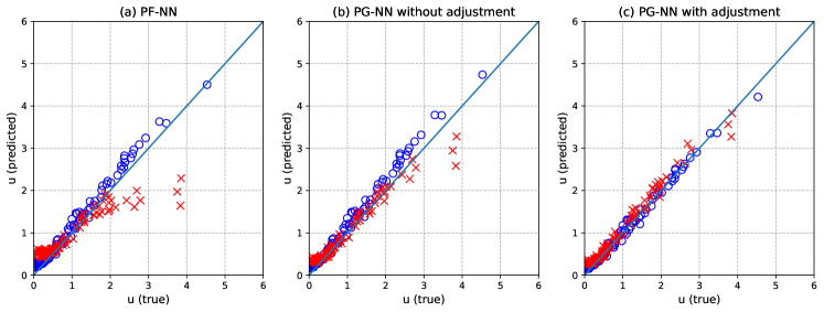
Theorem 1 shows that the adjustment (7) improves the random effect prediction. According to our experience, even though limited, this adjustment becomes important, especially when the cluster size is large. Figure 2 is the plot of against the true under and . Figure 2 (a) shows that the use of fixed effects for subject-specific effects (PF-NN) produces poor prediction of . Figure 2 (b) and (c) show that the use of random effects for subject-specific effects (PG-NN) improves the subject-specific prediction, and the proposed adjustment improves it further.
4.3 Pretraining variance components
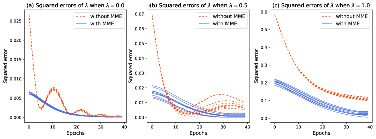
We found that the MLE for variance component could be sensitive to the choice of initial value, giving a slow convergence. We propose the use of method-of-moments estimator (MME) for pretraining ,
| (8) |
where . Convergence of the MME (8) is shown in Appendix A.3. Figure 3 shows that the proposed pretraining accelerates the convergence in various settings. In Appendix A.4, we demonstrate an additional experiments for verifying the consistency of of the proposed method.
4.4 Feature Selection in High Dimensional Settings
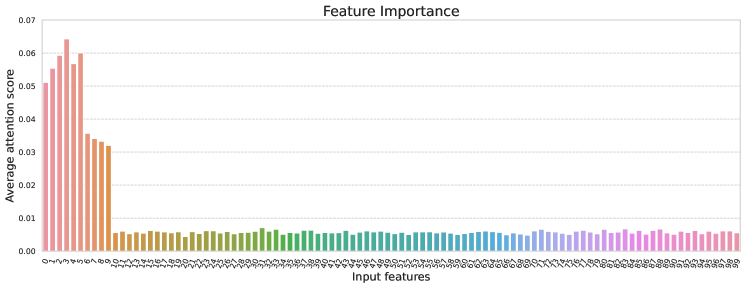
Feature selection methods can be easily implemented to the proposed PG-NN. As an example, we implemented feature selection using the multi-head attention layer with sparsemax function (Martins and Astudillo,, 2016; Škrlj et al.,, 2020; Arik and Pfister,, 2021),
where . As a high dimensional setting, we generate input features from for , including 10 genuine features and 90 irrelevant features . The output is generated from with the mean model,
where is generated from . The number of subjects is , i.e. the cardinality of the categorical feature is . The number of repeated measures (cluster size) is set to be , which is smaller than number of features . We employed a multi-layer perceptron with 20-10-10 number of nodes and three-head attention layer for feature selection. Other details are derived in Section 5. Figure 4 shows the average attention scores of 50 repetitions. It is evident that all the genuine features are ranked at the top 10.
5 Experimental Studies
To investigate the performance of the Poisson-gamma DNN, we conducted experimental studies. The five input variables are generated from the AR(1) process with autocorrelation for each and . The random effects are generated from either or where . When , the conditional mean is identical to the marginal mean . The output variable is generated from Poisson with
Results are based on the 100 sets of simulated data. The data consist of observations for subjects. For each subject, 6 observations are assigned to the training set, 2 are assigned to the validation set, and the remaining 2 are assigned to the test set.
For comparison, we consider the following models.
-
•
P-GLM Classic Poisson GLM for count outputs using R.
-
•
N-NN Conventional DNN for continuous outputs.
-
•
P-NN Poisson DNN for count outputs.
-
•
PN-GLM Poisson-normal HGLM using lme4 (Bates et al.,, 2015) package in R.
-
•
PG-GLM Poisson-gamma HGLM using the proposed method.
-
•
NF-NN Conventional DNN with fixed subject-specific effects for continuous outputs.
-
•
NN-NN DNN with normal random effects for continuous outputs (Lee and Lee,, 2023).
-
•
PF-NN Conventional Poisson DNN with fixed subject-specific effects for count outputs.
-
•
PG-NN The proposed Poisson-gamma DNN for count outputs.
To evaluate the prediction performances, we consider the root mean squared Pearson error (RMSPE)
where and is a dispersion parameter of GLM family. For Gaussian outputs, the RMSPE is identical to the ordinary root mean squared error, since and . For Poisson outputs, since and , the RMSPE for test set is given by
P-GLM, N-NN, and P-NN give marginal predictions , while the others give subject-specific predictions . N-NN, NF-NN, and NN-NN are models for continuous outputs, while the others are models for count outputs. For NF-NN and PF-NN, predictions are made by maximizing the conditional likelihood . On the other hand, for PN-GLM, PG-GLM, NN-NN, and PG-NN, subject-specific predictions are made by maximizing the h-likelihood.
PN-GLM is the generalized linear mixed model with random effects . Current statistical software for PN-GLM and PG-GLM (lme4 and dhglm) provide approximate MLEs using Laplace approximation. The proposed learning algorithm can yield exact MLEs for PG-GLM, using solely the input and output layers while excluding the hidden layers. Among various methods for NN-NN (Tran et al.,, 2020; Mandel et al.,, 2023; Simchoni and Rosset,, 2021, 2023; Lee and Lee,, 2023), we applied the state-of-the-art method proposed by Lee and Lee, (2023). All the DNNs and PG-GLMs were implemented in Python using Keras (Chollet et al.,, 2015) and TensorFlow (Abadi et al.,, 2015). For all DNNs, we employed a standard multi-layer perceptron (MLP) consisting of 3 hidden layers with 10 neurons and leaky ReLU activation function. We applied the Adam optimizer with a learning rate of 0.001 and an early stopping process based on the validation loss while training the DNNs. NVIDIA Quadro RTX 6000 were used for computations.
| Distribution of random effects () | |||||
|---|---|---|---|---|---|
| Model | G(0) & N(0) | G(0.5) | G(1) | N(0.5) | N(1) |
| P-GLM | 1.046 (0.029) | 1.501 (0.055) | 1.845 (0.085) | 1.745 (0.113) | 2.818 (0.467) |
| N-NN | 1.013 (0.018) | 1.473 (0.042) | 1.816 (0.074) | 1.713 (0.097) | 1.143 (0.432) |
| P-NN | 1.011 (0.018) | 1.470 (0.042) | 1.812 (0.066) | 1.711 (0.099) | 1.161 (0.440) |
| PN-GLM | 1.048 (0.029) | 1.112 (0.033) | 1.115 (0.035) | 1.124 (0.030) | 1.152 (0.034) |
| PG-GLM | 1.048 (0.020) | 1.123 (0.027) | 1.106 (0.023) | 1.139 (0.026) | 1.161 (0.028) |
| NF-NN | 1.152 (0.029) | 1.301 (0.584) | 1.136 (0.311) | 1.241 (1.272) | 1.402 (0.298) |
| NN-NN | 1.020 (0.020) | 1.121 (0.026) | 1.209 (0.067) | 1.256 (0.097) | 2.773 (0.384) |
| PF-NN | 1.147 (0.025) | 1.135 (0.029) | 1.128 (0.027) | 1.129 (0.024) | 1.128 (0.027) |
| PG-NN | 1.016 (0.019) | 1.079 (0.024) | 1.084 (0.023) | 1.061 (0.022) | 1.085 (0.026) |
Table 1 shows the mean and standard deviation of test RMSPEs from the experimental studies. When the true model does not have random effects (G(0) and N(0)), the PG-NN is comparable to the P-NN without random effects, which should perform the best (marked by the bold face) in terms of RMSPE. N-NN (P-NN) without random effects is also better than NF-NN and NN-NN (PF-NN and PG-NN) with random effects. When the distribution of random effects is correctly specified (G(0.5) and G(1)), the PG-NN performs the best in terms of RMSPE. Even when the distribution of random effects is misspecified (N(0.5), N(1)), the PG-NN still performs the best. This result is in accordance with the simulation results of McCulloch and Neuhaus, (2011), namely, in GLMMs, the prediction accuracy is little affected for violations of the distributional assumption for random effects: see similar performances of PN-GLM and PG-GLM.
It has been known that handling the high-cardinality categorical features as random effects has advantages over handling them as fixed effects (Lee et al.,, 2017), especially when the cardinality of categorical feature is close to the sample size, i.e., the number of observations in each category (cluster size ) is relatively small. Thus, to emphasize the advantages of PG-NN over PF-NN in high-cardinality categorical features, we consider two additional scenarios for experimental study with cluster size and where and . Mean and standard deviation of RMSPE of PF-NN are 1.269 (0.038) and 1.629 (0.086) for and , respectively. Those of PG-NN are 1.124 (0.028) and 1.284 (0.049) for each scenario. Therefore, the proposed method enhances subject-specific predictions as the cardinality of categorical features becomes high.
6 Real Data Analysis
| Dataset | |||||
|---|---|---|---|---|---|
| Model | Epilepsy | CD4 | Bolus | Owls | Fruits |
| P-GLM | 1.520 | 6.115 | 2.110 | 2.307 | 6.818 |
| N-NN | 2.119 | 8.516 | 1.982 | 2.297 | 6.573 |
| P-NN | 1.712 | 6.830 | 2.354 | 3.076 | 6.854 |
| PN-GLM | 1.242 | 3.422 | 1.727 | 5.791 | 6.795 |
| PG-GLM | 1.229 | 4.424 | 1.714 | 4.479 | 5.786 |
| NF-NN | 1.750 | 6.921 | 1.718 | 2.215 | 5.897 |
| NN-NN | 1.770 | 7.640 | 1.727 | 2.674 | 5.825 |
| PF-NN | 1.238 | 3.558 | 1.816 | 2.951 | 6.430 |
| PG-NN | 1.135 | 3.513 | 1.677 | 2.000 | 6.376 |
To investigate the prediction performance of clustered count outputs in practice, we examined the following five real datasets:
For all the DNNs, a standard MLP with one hidden layer of 10 neurons and a sigmoid activation function were employed. For longitudinal data (Epilepsy, CD4, Bolus), the last observation for each patient was used as the test set. For clustered data (Owls, Fruits), an observation was randomly selected as the test set from each cluster. RMSPEs are reported in Table 2, which shows that the use of subject-specific models (PG-NN and PG-GLM) for count data are the best. Throughout the datasets, P-GLM performs better than P-NN, implying that non-linear model does not improve the linear model in the absence of subject-specific random effects. Meanwhile, in the presence of subject-specific random effects, PG-NN is always preferred to PG-GLM except for Fruits data. The results imply that introducing subject-specific random effects in DNNs can help to identify the nonlinear effects of the input variables. Therefore, while DNNs are widely recognized for improving predictions in independent datasets, introducing subject-specific random effects could be necessary for DNNs to improve their predictions in correlated datasets with high-cardinality categorical features.
7 Concluding Remarks
When the data contains high-cardinality categorical features, introducing random effects into DNNs is advantageous. We develop subject-specific Poisson-gamma DNN for clustered count data. The h-likelihood enables a fast end-to-end learning algorithm using the single objective function. By introducing subject-specific random effects, DNNs can effectively identify the nonlinear effects of the input variables. Various state-of-the-art network architectures can be easily implemented into the h-likelihood framework, as we demonstrate with the feature selection based on multi-head attention.
References
- Abadi et al., (2015) Abadi, M., Agarwal, A., Barham, P., Brevdo, E., Chen, Z., Citro, C., Corrado, G. S., Davis, A., Dean, J., Devin, M., Ghemawat, S., Goodfellow, I., Harp, A., Irving, G., Isard, M., Jia, Y., Jozefowicz, R., Kaiser, L., Kudlur, M., Levenberg, J., Mané, D., Monga, R., Moore, S., Murray, D., Olah, C., Schuster, M., Shlens, J., Steiner, B., Sutskever, I., Talwar, K., Tucker, P., Vanhoucke, V., Vasudevan, V., Viégas, F., Vinyals, O., Warden, P., Wattenberg, M., Wicke, M., Yu, Y., and Zheng, X. (2015). TensorFlow: Large-scale machine learning on heterogeneous systems.
- Arik and Pfister, (2021) Arik, S. Ö. and Pfister, T. (2021). Tabnet: Attentive interpretable tabular learning. In Proceedings of the AAAI conference on artificial intelligence, volume 35, pages 6679–6687.
- Banta et al., (2010) Banta, J. A., Stevens, M. H., and Pigliucci, M. (2010). A comprehensive test of the ‘limiting resources’ framework applied to plant tolerance to apical meristem damage. Oikos, 119(2):359–369.
- Bates et al., (2015) Bates, D., Mächler, M., Bolker, B., and Walker, S. (2015). Fitting linear mixed-effects models using lme4. Journal of Statistical Software, 67(1):1–48.
- Bishop and Nasrabadi, (2006) Bishop, C. M. and Nasrabadi, N. M. (2006). Pattern recognition and machine learning, volume 4. Springer.
- Blei et al., (2017) Blei, D. M., Kucukelbir, A., and McAuliffe, J. D. (2017). Variational inference: A review for statisticians. Journal of the American statistical Association, 112(518):859–877.
- Breslow and Clayton, (1993) Breslow, N. E. and Clayton, D. G. (1993). Approximate inference in generalized linear mixed models. Journal of the American statistical Association, 88(421):9–25.
- Brooks et al., (2023) Brooks, M., Bolker, B., Kristensen, K., Maechler, M., Magnusson, A., McGillycuddy, M., Skaug, H., Nielsen, A., Berg, C., Bentham, o. v., Sadat, N., Lüdecke, D., Lenth, R., O’Brien, J., Geyer, C. J., Jagan, M., Wiernik, B., and Stouffer, D. B. (2023). glmmTMB: Generalized Linear Mixed Models using Template Model Builder. R package version 3.2.0.
- Chollet et al., (2015) Chollet, F. et al. (2015). Keras.
- Dauphin et al., (2014) Dauphin, Y. N., Pascanu, R., Gulcehre, C., Cho, K., Ganguli, S., and Bengio, Y. (2014). Identifying and attacking the saddle point problem in high-dimensional non-convex optimization. Advances in neural information processing systems, 27.
- Gilmour et al., (1985) Gilmour, A., Anderson, R. D., and Rae, A. L. (1985). The analysis of binomial data by a generalized linear mixed model. Biometrika, 72(3):593–599.
- Goodfellow et al., (2016) Goodfellow, I., Bengio, Y., and Courville, A. (2016). Deep learning. MIT press.
- Harville and Mee, (1984) Harville, D. A. and Mee, R. W. (1984). A mixed-model procedure for analyzing ordered categorical data. Biometrics, pages 393–408.
- Henderson et al., (1959) Henderson, C. R., Kempthorne, O., Searle, S. R., and Von Krosigk, C. (1959). The estimation of environmental and genetic trends from records subject to culling. Biometrics, 15(2):192–218.
- Henderson and Shimakura, (2003) Henderson, R. and Shimakura, S. (2003). A serially correlated gamma frailty model for longitudinal count data. Biometrika, 90(2):355–366.
- Henry et al., (1998) Henry, K., Erice, A., Tierney, C., Balfour Jr, H., Fischl, M., Kmack, A., Liou, S., Kenton, A., Hirsch, M., Phair, J., et al. (1998). A randomized, controlled, double-blind study comparing the survival benefit of four different reverse transcriptase inhibitor therapies (three-drug, two-drug, and alternating drug) for the treatment of advanced aids. Journal of Acquired Immune Deficiency Syndromes and Human Retrovirology, 19:339–349.
- LeCun et al., (2015) LeCun, Y., Bengio, Y., and Hinton, G. (2015). Deep learning. Nature, 521(7553):436–444.
- Lee and Lee, (2023) Lee, H. and Lee, Y. (2023). H-likelihood approach to deep neural networks with temporal-spatial random effects for high-cardinality categorical features. In Proceedings of the 40th International Conference on Machine Learning, volume 202, pages 18974–18987. PMLR.
- Lee and Nelder, (1996) Lee, Y. and Nelder, J. A. (1996). Hierarchical generalized linear models. Journal of the Royal Statistical Society: Series B (Methodological), 58(4):619–656.
- Lee and Nelder, (2001) Lee, Y. and Nelder, J. A. (2001). Hierarchical generalised linear models: a synthesis of generalised linear models, random-effect models and structured dispersions. Biometrika, 88(4):987–1006.
- Lee et al., (2017) Lee, Y., Nelder, J. A., and Pawitan, Y. (2017). Generalized linear models with random effects: unified analysis via H-likelihood. Chapman and Hall/CRC.
- Mandel et al., (2023) Mandel, F., Ghosh, R. P., and Barnett, I. (2023). Neural networks for clustered and longitudinal data using mixed effects models. Biometrics, 79(2):711–721.
- Martins and Astudillo, (2016) Martins, A. and Astudillo, R. (2016). From softmax to sparsemax: A sparse model of attention and multi-label classification. In International conference on machine learning, pages 1614–1623. PMLR.
- McCulloch and Neuhaus, (2011) McCulloch, C. E. and Neuhaus, J. M. (2011). Prediction of random effects in linear and generalized linear models under model misspecification. Biometrics, 67(1):270–279.
- Rodrigo and Tsokos, (2020) Rodrigo, H. and Tsokos, C. (2020). Bayesian modelling of nonlinear poisson regression with artificial neural networks. Journal of Applied Statistics, 47(5):757–774.
- Roulin and Bersier, (2007) Roulin, A. and Bersier, L.-F. (2007). Nestling barn owls beg more intensely in the presence of their mother than in the presence of their father. Animal Behaviour, 74(4):1099–1106.
- Schall, (1991) Schall, R. (1991). Estimation in generalized linear models with random effects. Biometrika, 78(4):719–727.
- Simchoni and Rosset, (2021) Simchoni, G. and Rosset, S. (2021). Using random effects to account for high-cardinality categorical features and repeated measures in deep neural networks. Advances in Neural Information Processing Systems, 34:25111–25122.
- Simchoni and Rosset, (2023) Simchoni, G. and Rosset, S. (2023). Integrating random effects in deep neural networks. Journal of Machine Learning Research, 24(156):1–57.
- Škrlj et al., (2020) Škrlj, B., Džeroski, S., Lavrač, N., and Petkovič, M. (2020). Feature importance estimation with self-attention networks. arXiv preprint arXiv:2002.04464.
- Thall and Vail, (1990) Thall, P. F. and Vail, S. C. (1990). Some covariance models for longitudinal count data with overdispersion. Biometrics, pages 657–671.
- Tran et al., (2020) Tran, M.-N., Nguyen, N., Nott, D., and Kohn, R. (2020). Bayesian deep net GLM and GLMM. Journal of Computational and Graphical Statistics, 29(1):97–113.
- Wolfinger, (1993) Wolfinger, R. (1993). Laplace’s approximation for nonlinear mixed models. Biometrika, 80(4):791–795.
Appendix A Appendix
A.1 Derivation of the h-likelihood
Maximizing with respect to yields,
where and . As derived in Section 3, define as
and consider a transformation,
Since the multiplier does not depend on , we have
which leads to
This satisfies the sufficient condition for the h-likelihood to give exact MLEs for fixed parameters,
Furthermore, from the distribution of ,
and
Therefore, maximizing the h-likelihood yields the BUPs of and .
A.2 Proof of Theorem 1.
A.3 Convergence of the method-of-moments estimator
As derived in Section A, for given and , maximization of the h-likelihood leads to
Thus, and . Define as
to have and for any . Then, by the law of large numbers,
Note here that
Then, solving the following equation,
leads to an estimate in (8) and as .
A.4 Consistency of variance component estimator
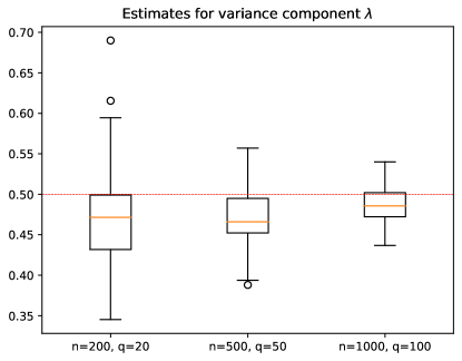
By jointly maximizing the proposed h-likelihood, we obtain MLEs for fixed parameters and BUPs for random parameters. Thus, we can directly apply the consistency of MLEs under usual regularity conditions. To verify this consistency in PG-NN, we present the boxplots in Figure 5 for the variance component estimator from 100 repetitions with true . The number of clusters and cluster size are set to be (200, 20), (500, 50), and (1000,100). Figure 5 provide conclusive evidence confirming the consistency of the variance component estimator within the PG-NN framework.
A.5 Details of the real datasets
-
•
Epilepsy data: Epilepsy data are reported by Thall and Vail, (1990) from a clinical trial of patients with epilepsy. The data contain observations with repeated measures from each patient and input variables.
-
•
CD4 data: CD4 data are from a study of AIDS patients with advanced immune suppression, reported by Henry et al., (1998). The data contain observations from patients with repeated measurements and input variables.
-
•
Bolus data: Bolus data are from a clinical trial following abdominal surgery for patients with repeated measurements, reported in Henderson and Shimakura, (2003). The data have observations with input variables.
- •
-
•
Fruits data: Fruits data are reported in Banta et al., (2010). The data have observations clustered by types of maternal seed family with input variables. The cluster size varies from 11 to 47.