Adaptive Bootstrap Tests for Composite Null Hypotheses in the Mediation Pathway Analysis

Abstract

Mediation analysis aims to assess if, and how, a certain exposure influences an outcome of interest through intermediate variables. This problem has recently gained a surge of attention due to the tremendous need for such analyses in scientific fields. Testing for the mediation effect is greatly challenged by the fact that the underlying null hypothesis (i.e. the absence of mediation effects) is composite. Most existing mediation tests are overly conservative and thus underpowered. To overcome this significant methodological hurdle, we develop an adaptive bootstrap testing framework that can accommodate different types of composite null hypotheses in the mediation pathway analysis. Applied to the product of coefficients (PoC) test and the joint significance (JS) test, our adaptive testing procedures provide type I error control under the composite null, resulting in much improved statistical power compared to existing tests. Both theoretical properties and numerical examples of the proposed methodology are discussed.

1 Introduction

Mediation analysis plays a crucial role in investigating the underlying mechanism or pathway between an exposure and an outcome through an intermediate variable called a mediator (MacKinnon, 2008; VanderWeele, 2015). It decomposes the “total effect” of an exposure on an outcome into an indirect effect that is through a given mediator and a direct effect, not through the mediator. The former holds the key to uncovering the exposure-outcome mechanism and is often known as the mediation effect. The mediation effect was initially studied under structural equation models (SEMs) in social sciences (Sobel, 1982; Baron and Kenny, 1986) and has been given formal causal definitions (Robins and Greenland, 1992; Pearl, 2001; Imai et al., 2010b) within the counterfactual framework (Imbens and Rubin, 2015). Examining the presence or absence of the mediation effect can facilitate a deeper understanding of the underlying causal pathway from the exposure to the outcome and can give essential insights into intervention consequences, e.g., manipulating the mediator to change the exposure-outcome mechanism. As a result, it is of interest to apply mediation analysis in many scientific fields, such as psychology (MacKinnon and Fairchild, 2009; Valeri and VanderWeele, 2013), genomics (Zhao et al., 2014; Huang and Pan, 2016; Huang, 2018; Guo et al., 2022), and epidemiology (Barfield et al., 2017; Fulcher et al., 2019), among others.

To analyze the mediation effect, one classical setting models the relationship between the exposure, the potential mediator, and the outcome as a directed acyclic graph; see Figure 1.

Figure 1: Directed Acyclic Graph for Mediation Analysis. The exposure is $S$; the mediator is $M$; the outcome is $Y$; the potential confounders are $X$.

Specifically, let $\alpha_{S}$ parametrize the causal effect of the exposure on the mediator, and $\beta_{M}$ parametrize the causal effect of the mediator on the outcome conditioning on the exposure. Then in the classical linear SEM (Sobel, 1982; Baron and Kenny, 1986), the causal mediation effect is proportional to $\alpha_{S}\beta_{M}$ under suitable identification assumptions (Imai et al., 2010a). More generally, this product expression $\alpha_{S}\beta_{M}$ may also appear in the causal mediation effect under many other models, such as generalized linear models and survival analysis models (VanderWeele and Vansteelandt, 2010; VanderWeele, 2011; Huang and Cai, 2016). Therefore, the important scientific question of whether or not the mediation effect is absent can be formulated as the hypothesis testing problem $H_{0}:\alpha_{S}\beta_{M}=0$ against $H_{A}:\alpha_{S}\neq 0$ and $\beta_{M}\neq 0$ (MacKinnon, 2008). Note that $H_{0}:\alpha_{S}\beta_{M}=0$ holds if and only if $\alpha_{S}=0$ or $\beta_{M}=0$, corresponding to two parameter sets $\mathcal{P}_{\alpha}=\{(\alpha_{S},\beta_{M}):\alpha_{S}=0\}$ and $\mathcal{P}_{\beta}=\{(\alpha_{S},\beta_{M}):\beta_{M}=0\}$, respectively. It follows that the parameter set of $H_{0}:\alpha_{S}\beta_{M}=0$ is the union of two sets $\mathcal{P}_{\alpha}$ and $\mathcal{P}_{\beta}$. We visualize $\mathcal{P}_{\alpha}$, $\mathcal{P}_{\beta}$, and their union $\mathcal{P}_{\alpha}\cup\mathcal{P}_{\beta}$ in Figures 2(a)–2(c), respectively.

(a) $\alpha_{S}=0$

(b) $\beta_{M}=0$

(c) $\alpha_{S}\beta_{M}=0$

(d) $\alpha_{S}=\beta_{M}=0$

Figure 2: Visualization of parameter spaces of $(\alpha_{S},\beta_{M})$ under different constraints

To test $H_{0}:\alpha_{S}\beta_{M}=0$, a broad class of methods is based on the product of coefficients (PoC) $\hat{\alpha}_{S,n}\hat{\beta}_{M,n}$, where $\hat{\alpha}_{S,n}$ and $\hat{\beta}_{M,n}$ denote the sample estimates of parameters $\alpha_{S}$ and $\beta_{M}$, respectively. One popular PoC method is Sobel’s test (Sobel, 1982), which is a Wald-type test and approximates the variance of $\hat{\alpha}_{S,n}\hat{\beta}_{M,n}$ by the first-order Delta method. In addition, the joint significance (JS) test (Fritz and MacKinnon, 2007), also known as the MaxP test, is another widely used test that rejects the $H_{0}$ of no mediation effect if both $\hat{\alpha}_{S,n}$ and $\hat{\beta}_{M,n}$ pass a certain cutoff of statistical significance. Liu et al. (2021) pointed out that the MaxP test is a kind of likelihood ratio test under normality assumptions.

Although there are various procedures available for testing mediation effects, properly controlling the type I error remains a challenge due to the intrinsic structure of the null parameter space. In particular, $H_{0}:\alpha_{S}\beta_{M}=0$ is composed of three different parameter cases: (i) $\alpha_{S}=0$ and $\beta_{M}\neq 0$; (ii) $\alpha_{S}\neq 0$ and $\beta_{M}=0$; (iii) $\alpha_{S}=0$ and $\beta_{M}=0$. Case (iii), illustrated in Figure 2(d), is a singleton given by the intersection set $\mathcal{P}_{\alpha}\cap\mathcal{P}_{\beta}$. Under case (iii), both parameters $\alpha_{S}$ and $\beta_{M}$ are fixed at $0$, whereas cases (i) and (ii) have one fixed parameter and the other parameter to be estimated. This intrinsic difference leads to distinct asymptotic behaviors of test statistics. Since the underlying truth is typically unknown in practice, it is difficult to obtain proper $p$-values under the composite null hypothesis.

Particularly, in the popular Sobel’s test and the MaxP test, the asymptotic distributions of the test statistics under cases (i) and (ii) are known to be different from those under case (iii). These tests have been shown to be overly conservative in case (iii), because statistical inference is carried out according to the asymptotic distributions determined in cases (i) and (ii) (MacKinnon et al., 2002; Fritz and MacKinnon, 2007). This issue has gained a surge of attention in recent genome-wide epidemiological studies, where for the majority of omics markers, it holds that $\alpha_{S}=\beta_{M}=0$, and the classical tests are generally underpowered (Barfield et al., 2017). Some recent work (Liu et al., 2021; Dai et al., 2020; Du et al., 2022) utilized the relative proportions of the cases (i)–(iii) in the population, but they rely on accurate estimation of the true proportions. Huang (2019a, b) adjusted the composition of $H_{0}:\alpha_{S}\beta_{M}=0$ through the variances of test statistics but required that the non-zero coefficients are weak and sparse, which can be violated when the sample size is large. Another line of related research (Sampson et al., 2018; Djordjilović et al., 2019, 2020; Derkach et al., 2020) used a screening step to control the family-wise error rate or the false discovery rate for a large group of hypotheses, but they did not directly provide proper $p$-values for each of the composite null hypotheses. Van Garderen and Van Giersbergen (2022) proposed to construct a critical region for testing that can nearly control the type I error at one prespecified significance level. Miles and Chambaz (2021) construct a rejection region that can achieve type I error control at significance level $\omega$ with $\omega^{-1}$ a positive integer. Despite these developments, the fundamental issue of correctly characterizing the distributions of test statistics to obtain well-calibrated $p$-values under a composite null hypothesis remains an important challenging problem in the current literature of mediation analyses.

In this paper, we develop a new hypothesis testing methodology to address the challenge of obtaining uniformly distributed $p$-values under the composite null hypothesis of no mediation effect. Particularly, we propose an adaptive bootstrap procedure that can flexibly accommodate different types of null hypotheses. In the current literature, the nonparametric bootstrap is directly applied to the PoC test statistic $\hat{\alpha}_{S,n}\hat{\beta}_{M,n}$, which has been, unfortunately, found numerically to be overly conservative when $\alpha_{S}=\beta_{M}=0$ (Fritz and MacKinnon, 2007; Barfield et al., 2017). This paper unveils analytically the reason for the failure of the conventional nonparametric bootstrap method, which stems from non-regular limiting behaviors of the PoC test statistic at the neighborhood of $(\alpha_{S},\beta_{M})=(0,0)$. To overcome the non-regularity near $(\alpha_{S},\beta_{M})=(0,0)$, we derive an explicit representation of the asymptotic distribution of the PoC test statistic through a local model, and perform a consistent bootstrap estimation by incorporating suitable thresholds. In addition, for the JS test, we show that the conventional nonparametric bootstrap also fails to control type I error properly, which can be fixed by an adaptive bootstrap test similar to the procedure of the PoC test. For both the PoC test and the JS test, the proposed methods can circumvent the nonstandard limiting behaviors of the test statistics and therefore uniformly adapt to different types of null cases of no mediation effect.

The structure of this paper is as follows. In Section 2, we briefly review the basic problem setting and several popular testing methods in the literature. In Section 3, we introduce the adaptive bootstrap method that can be applied to the representative PoC and JS tests under classical linear SEMs. In Section 4, we conduct extensive simulation studies to compare the finite sample performances of the proposed tests with popular counterparts. In Section 6, we apply our adaptive bootstrap tests to investigate the mediation pathways of metabolites on the association of environmental exposures with a health outcome. In Section 5, we develop extensions of the adaptive bootstrap, including joint testing of multivariate mediators and testing mediation effects under non-linear models. We conclude the paper and discuss interesting extensions in Section 7.

Notation. For two sequences of real numbers $\{a_{n}\}$ and $\{b_{n}\}$, we write $a_{n}=o(b_{n})$ if $\lim_{n\to\infty}a_{n}/b_{n}=0$. We let $\xrightarrow{d}$ denote convergence in distribution. We let $\overset{d^{*}}{\leadsto}$ denote bootstrap consistency relative to the Kolmogorov-Smirnov distance; see an introduction of this consistency notion in Section 23 of van der Vaart (2000). To ensure clarity, we also provide the definitions of all the convergence modes in Section A of the Supplementary Material.

2 Hypothesis Tests of No Mediation Effect

Mediation Analysis Model.   To examine the mediation effect of the exposure $S$ on the outcome $Y$ through the intermediate variable $M$, the causal inference literature utilizes the counterfactual framework (VanderWeele, 2015). In particular, let $M(s)$ denote the potential value of the mediator under the exposure $S=s$, and let $Y(s,m)$ denote the potential outcome that would have been observed if $S$ and $M$ had been set to $s$ and $m$, respectively. Throughout the paper, we adopt the Stable Unit Treatment Value Assumption (Rubin, 1980), so that $M=M(S)$ and $Y=Y(S,M(S))$. Then the mediation effect or the natural indirect effect of $S=s$ versus $s^{*}$ (Imai et al., 2010b) is defined as

$$\mathrm{E}\big{\{}Y(s,M(s))-Y(s,M(s^{*}))\big{\}}.$$ (1)

For ease of illustration, we consider the popular linear Structural Equation Model (SEM) (MacKinnon, 2008; VanderWeele, 2015):

$$M = \alpha_{S}S+\boldsymbol{X}^{\top}\boldsymbol{\alpha}_{\boldsymbol{X}}+\epsilon_{M},$$ (2)

$$Y = \beta_{M}M+\boldsymbol{X}^{\top}\boldsymbol{\beta}_{\boldsymbol{X}}+\tau_{S}S+\epsilon_{Y},$$

where $\boldsymbol{X}$ denotes a vector of confounders with the first element being 1 for the intercept, and $\epsilon_{Y}$ and $\epsilon_{M}$ are independent error terms with mean zero and finite variances $\sigma_{\epsilon_{Y}}^{2}$ and $\sigma_{\epsilon_{M}}^{2}$, respectively. We assume that there are $n$ independent and identically distributed (i.i.d.) observations, $\{(S_{i},\boldsymbol{X}_{i},M_{i},Y_{i}):i=1,\ldots,n\}$, sampled from Model (2). The independence of $\epsilon_{Y}$ and $\epsilon_{M}$ holds under the following no unmeasured confounding assumptions. In particular, let $A\perp B\mid C$ denote the independence of $A$ and $B$ conditional on $C$, and we assume that for all levels of $s,s^{*}$ and $m$, (i) $Y(s,m)\perp S\mid\{\boldsymbol{X}=\boldsymbol{x}\}$, no confounder for the relation of $Y$ and $S$; (ii) $Y(s,m)\perp M\mid\{S=s,\boldsymbol{X}=\boldsymbol{x}\}$, no confounder for the relation of $Y$ and $M$ conditioning on $S=s$; (iii) $M(s)\perp S\mid\{\boldsymbol{X}=\boldsymbol{x}\}$, no confounder for the relation of $M$ and $S$; (iv) $Y(s,m)\perp M(s^{*})\mid\{\boldsymbol{X}=\boldsymbol{x}\}$, no confounder for the $M$-$Y$ relation that is affected by $S$ (VanderWeele and Vansteelandt, 2009). Under these assumptions, the model can be visualized by the directed acyclic graph in Figure 1, and the mediation effect $\eqref{eq:MEpotential}$ equals $\alpha_{S}\beta_{M}(s-s^{*})$.

Therefore, the scientific goal of detecting the presence of a mediation effect can be formulated as the following hypothesis testing problem:

$$H_{0}:\alpha_{S}\beta_{M}=0\quad\text{\ versus\ }\quad H_{A}:\alpha_{S}\beta_{M}\neq 0.$$

This null hypothesis is composite and can be decomposed into three disjoint cases:

$$H_{0}:\begin{cases}H_{0,1}:&\alpha_{S}=0,~{}\beta_{M}\neq 0;\\ H_{0,2}:&\alpha_{S}\neq 0,~{}\beta_{M}=0;\\ H_{0,3}:&\alpha_{S}=\beta_{M}=0,\end{cases}$$ (3)

and the alternative hypothesis is $H_{A}:\alpha_{S}\neq 0\text{ and }\beta_{M}\neq 0.$

Remark 1

Composite null problems similar to (3) can occur in settings other than Model (2); the latter is considered to demonstrate the essential analytic details useful for possible generalizations. Similar issues have also been observed in many other scenarios, including partially linear models (Hines et al., 2021), survival analysis (VanderWeele, 2011), and high-dimensional models (Zhou et al., 2020). The analytic details of the methodology development in this paper can pave the path for useful generalizations to other important statistical models and applications.

To test the composite null (3), various methods have been proposed, and a comprehensive survey can be found in MacKinnon et al. (2002). There are two representative classes of tests: (I) the product of coefficients (PoC) test, which corresponds to a Wald-type test, and (II) the joint significance (JS) test, which is the likelihood ratio test under normality of the error terms (Liu et al., 2021). (I) The first class of methods examine the PoC: $\hat{\alpha}_{S,n}\hat{\beta}_{M,n}$, where $\hat{\alpha}_{S,n}$ and $\hat{\beta}_{M,n}$ denote consistent estimates of $\alpha_{S}$ and $\beta_{M}$, respectively. One common practice is to apply a normal approximation to $\hat{\alpha}_{S,n}\hat{\beta}_{M,n}$ divided by its standard error, where Sobel (1982) derives the standard error formula by the first-order Delta method. In addition to the large-sample approximation, the bootstrap has also been used to evaluate the distribution of $\hat{\alpha}_{S,n}\hat{\beta}_{M,n}$ (MacKinnon et al., 2004; Fritz and MacKinnon, 2007). (II) The JS test, also known as the MaxP test, rejects $H_{0}:\alpha_{S}\beta_{M}=0$ if $\max\{p_{\alpha_{S}},p_{\beta_{M}}\}<\omega$, where $\omega$ is a prespecified significance level, and $p_{\alpha_{S}}$ and $p_{\beta_{M}}$ denote the $p$-values for $H_{0}:\alpha_{S}=0$ (the link $S\rightarrow M$) and $H_{0}:\beta_{M}=0$ (the link $M\rightarrow Y$), respectively. Despite their popularity, these methods have been found numerically to be overly conservative under $H_{0,3}$ in (3) (MacKinnon et al., 2002; Barfield et al., 2017). See a further discussion on the non-regular asymptotic behaviors of statistics underlying the conservatism in Section 3.

Similar issues have also been broadly recognized for Wald tests in various statistical problems including three-way contingency table analysis and factor analysis (Glonek, 1993; Dufour et al., 2013; Drton and Xiao, 2016). However, characterizing non-regular asymptotic behaviors under the singular null hypothesis $H_{0,3}$ is still insufficient to address intrinsic technical challenges in testing (3). In particular, the composite null (3) includes not only the singular case $H_{0,3}$ but also the other two non-singular cases $H_{0,1}$ and $H_{0,2}$. Since a test statistic follows different distributions under different null cases, and the underlying true null case is unknown, it is difficult to obtain uniformly distributed $p$-values through one simple asymptotic distribution under (3). To address this technical difficulty, we adopt, justify, and evaluate an adaptive bootstrap procedure. For both Wald-type PoC test and non-Wald JS test, we will show that the proposed procedure can naturally adapt to the three types of null hypotheses in (3) and yield uniformly distributed $p$-values across all different null cases.

3 Adaptive Bootstrap Tests

In this section, we propose a general Adaptive Bootstrap (AB) procedure for testing the composite null hypothesis (3). For illustration, we apply the adaptive bootstrap to the representative PoC test and show it can address the non-regularity issue. We emphasize that this general strategy can be applied in a wide range of scenarios. We also derive adaptive bootstrap procedure in other examples, including the Joint Significance test (Section B in the Supplementary Material), joint testing of multivariate mediators (Section 5.1) and testing mediation effect under the generalized linear models (Sections 5.2 and 5.3.).

To conduct hypothesis testing or estimate confidence intervals for statistics whose limiting distributions deviate from the normal, a simple and powerful approach is to apply the bootstrap resampling technique. However, the classical bootstrap is not a panacea, and on some occasions it can fail to work properly, including unfortunately the non-regular scenarios considered in this paper. In particular, it has been observed through simulation studies that the classical bootstrap technique is overly conservative under $H_{0,3}:\alpha_{S}=\beta_{M}=0$ (MacKinnon et al., 2002; Barfield et al., 2017). We next unveil the key insights underlying the failure of the classical bootstrap, which motivates our use of the adaptive bootstrap.

Non-Regularity of the PoC Test.  When $(\alpha_{S},\beta_{M})\neq(0,0)$, one of the first-order gradients $\frac{\partial\alpha_{S}\beta_{M}}{\partial\alpha_{S}}=\beta_{M}$ and $\frac{\partial\alpha_{S}\beta_{M}}{\partial\beta_{M}}=\alpha_{S}$ is nonzero. Thus the Delta method can be applied to support the use of Sobel’s test (based on asymptotic normality) and classical bootstrap (Barfield et al., 2017). However, under $H_{0,3}:(\alpha_{S},\beta_{M})=(0,0)$, the gradients $\frac{\partial\alpha_{S}\beta_{M}}{\partial\alpha_{S}}=\frac{\partial\alpha_{S}\beta_{M}}{\partial\beta_{M}}=0$, and validity of Sobel’s test and the classical bootstrap cannot be obtained as above.

We next illustrate the non-regular limiting behavior of the PoC $\hat{\alpha}_{S,n}\hat{\beta}_{M,n}$ under $H_{0,3}$. For ease of exposition, consider a special case of (2): $M=\alpha_{S}S+\epsilon_{M},$ and $Y=\beta_{M}M+\epsilon_{Y}.$ Let $(\hat{\alpha}_{S,n},\hat{\beta}_{M,n})$ denote the ordinary least squares estimators of $(\alpha_{S},\beta_{M})$, and let $(\hat{\alpha}_{S,n}^{*},\hat{\beta}_{M,n}^{*})$ the corresponding nonparametric bootstrap estimators. Here and throughout this paper, we use the superscript “$*$” to indicate estimators obtained from the nonparametric bootstrap, namely “bootstrap in pairs” in the regression setting. By classical asymptotic theory (van der Vaart, 2000), under mild conditions,

$$\sqrt{n}(\hat{\alpha}_{S,n}-\alpha_{S},\,\hat{\beta}_{M,n}-\beta_{M})^{\top}\xrightarrow{d}(Z_{S,0},\,Z_{M,0})^{\top},$$ (4)

where $(Z_{S,0},Z_{M,0})^{\top}$ denotes a mean-zero normal random vector with a covariance matrix given by that of the random vector $(\epsilon_{M}S/V_{S,0},\epsilon_{Y}M/V_{M,0})^{\top}$, $V_{S,0}=\mathrm{E}(S^{2})$, $V_{M,0}=\mathrm{E}(M^{2})$.

Moreover,

$$\sqrt{n}(\hat{\alpha}_{S,n}^{*}-\hat{\alpha}_{S,n},\hat{\beta}_{M,n}^{*}-\hat{\beta}_{M,n})^{\top}\overset{d^{*}}{\leadsto}(Z_{S,0}^{\prime},\,Z_{M,0}^{\prime})^{\top},$$ (5)

where $(Z_{S,0}^{\prime},Z_{M,0}^{\prime})$ is an independent copy of $(Z_{S,0},Z_{M,0})$ in (4) under the same distribution. By (4), $n(\hat{\alpha}_{S}\hat{\beta}_{M}-\alpha_{S}\beta_{M})\xrightarrow{d}Z_{S,0}Z_{M,0}$ under $H_{0,3}$, with the convergence rate $n$ different from the standard parametric $\sqrt{n}$ rate. By (4)–(5), we have $n(\hat{\alpha}_{S,n}^{*}\hat{\beta}_{M,n}^{*}-\hat{\alpha}_{S,n}\hat{\beta}_{M,n})=n\{(\hat{\alpha}_{S,n}^{*}-\hat{\alpha}_{S,n})\hat{\beta}_{M,n}+(\hat{\beta}_{M,n}^{*}-\hat{\beta}_{M,n})\hat{\alpha}_{S,n}+(\hat{\alpha}_{S,n}^{*}-\hat{\alpha}_{S})(\hat{\beta}_{M,n}^{*}-\hat{\beta}_{M,n})\}\overset{d^{*}}{\leadsto}{Z_{S,0}^{\prime}Z_{M,0}}+{Z_{S,0}Z_{M,0}^{\prime}}+{Z_{S,0}^{\prime}Z_{M,0}^{\prime}}.$ We can see that the limit of $n(\hat{\alpha}_{S,n}^{*}\hat{\beta}_{M,n}^{*}-\hat{\alpha}_{S,n}\hat{\beta}_{M,n})$ is different from that of $n(\hat{\alpha}_{S,n}\hat{\beta}_{M,n}-\alpha_{S}\beta_{M})$, implying inconsistency of the classical nonparametric bootstrap.

Adaptive Bootstrap of the PoC Test. To address the challenge of correctly evaluating the distribution of the PoC statistic, we utilize the local asymptotic analysis framework. Intuitively, the goal is to evaluate if a small change in the target parameters leads to little change on the limit of the statistics. To this end, given targeted parameters $(\alpha_{S},\beta_{M})$, we define their locally perturbed counterparts as $\alpha_{S,n}=\alpha_{S}+n^{-1/2}b_{\alpha}$, and $\beta_{M,n}=\beta_{M}+n^{-1/2}b_{\beta}$, respectively, where $(b_{\alpha},b_{\beta})$ denote the local parameters of perturbations from our targeted coefficients $(\alpha_{S},\beta_{M}).$ We then frame the problem under the local linear SEM as follows:

$$M = \alpha_{S,n}S+\boldsymbol{X}^{\top}\boldsymbol{\alpha}_{\boldsymbol{X}}+\epsilon_{M},\hskip 15.00002ptY=\beta_{M,n}M+\boldsymbol{X}^{\top}\boldsymbol{\beta}_{\boldsymbol{X}}+\tau_{S}S+\epsilon_{Y},$$ (6)

where $\epsilon_{M}$ and $\epsilon_{Y}$ are independent error terms with mean zero and finite variances. Fixing the target parameters $(\alpha_{S},\beta_{M})$, according to van der Vaart (2000) the formulation given in (6) may also be viewed as a local statistical experiment with local parameters $(b_{\alpha},b_{\beta})$ under which we are interested in examining the limit of test statistics. Note that with the local parameters $(b_{\alpha},b_{\beta})=(0,0)$, (6) reduces to the original model (2) with the parameters $(\alpha_{S},\beta_{M})$. Our inference goal remains the same: that is, to test the underlying true coefficients $(\alpha_{S},\beta_{M})$. Technically, we consider a $\sqrt{n}$-vicinity of local neighboring values $(\alpha_{S,n},\beta_{M,n})$ only for the theoretical investigation of local asymptotic behaviors. Such an idea has also been used for studying other non-regularity issues (McKeague and Qian, 2015; Wang et al., 2018, etc.). To examine the limit of $\hat{\alpha}_{S,n}\hat{\beta}_{M,n}-\alpha_{S,n}\beta_{M,n}$ under (6), we assume the following general regularity Condition 1.

Condition 1

(C1.1) $\mathrm{E}(\epsilon_{M}|\boldsymbol{X},S)=0$ and $\mathrm{E}(\epsilon_{Y}|\boldsymbol{X},S,M)=0$. (C1.2) $\mathrm{E}(\boldsymbol{D}\boldsymbol{D}^{\top})$ is a positive definite matrix with bounded eigenvalues, where $\boldsymbol{D}=(\boldsymbol{X}^{\top},M,S)^{\top}$. (C1.3) The second moments of $(\epsilon_{M},\epsilon_{Y},S_{\perp},M_{\perp^{\prime}},\epsilon_{M}S_{\perp},\epsilon_{Y}M_{\perp^{\prime}})$ are finite, where $S_{\perp}=S-\boldsymbol{X}^{\top}Q_{1,S}$ with $Q_{1,S}=\{\mathrm{E}(\boldsymbol{X}\boldsymbol{X}^{\top})\}^{-1}\times\mathrm{E}(\boldsymbol{X}S)$, and $M_{\perp^{\prime}}=M-\tilde{\boldsymbol{X}}^{\top}Q_{2,M}$ with $\tilde{\boldsymbol{X}}=(\boldsymbol{X}^{\top},S)^{\top}$ and $Q_{2,M}=\{\mathrm{E}(\tilde{\boldsymbol{X}}^{\top}\tilde{\boldsymbol{X}})\}^{-1}\times\mathrm{E}(\tilde{\boldsymbol{X}}M)$.

Similarly to our above discussions under the simplified model, Theorem 1 establishes the limits of $\sqrt{n}\times(\hat{\alpha}_{S,n}\hat{\beta}_{M,n}-\alpha_{S}\beta_{M})$ and $n\times(\hat{\alpha}_{S,n}\hat{\beta}_{M,n}-\alpha_{S}\beta_{M})$ when $(\alpha_{S},\beta_{M})\neq(0,0)$ and $(\alpha_{S},\beta_{M})=(0,0)$, respectively.

Theorem 1 (Asymptotic Property)

Assume Condition 1. Under the local model (6),

1. when $(\alpha_{S},\beta_{M})\neq(0,0)$, $\sqrt{n}\times(\hat{\alpha}_{S,n}\hat{\beta}_{M,n}-\alpha_{S,n}\beta_{M,n})\xrightarrow{d}\alpha_{S}{Z_{M}}+\beta_{M}{Z_{S}};$

2. when $(\alpha_{S},\beta_{M})=(0,0)$, $n\times(\hat{\alpha}_{S,n}\hat{\beta}_{M,n}-\alpha_{S,n}\beta_{M,n})\xrightarrow{d}b_{\alpha}{Z_{M}}+b_{\beta}{Z_{S}}+{Z_{M}Z_{S}},$

where $(Z_{S},Z_{M})^{\top}$ is a mean-zero normal random vector with a covariance matrix given by that of the random vector $(\epsilon_{M}S_{\perp}/V_{S},\epsilon_{Y}M_{\perp^{\prime}}/V_{M})^{\top}$ with $V_{S}=\mathrm{E}(S_{\perp}^{2})$, and $V_{M}=\mathrm{E}(M_{\perp^{\prime}}^{2})$.

Theorem 1 suggests the limit of $\sqrt{n}(\hat{\alpha}_{S,n}\hat{\beta}_{M,n}-\alpha_{S,n}\beta_{M,n})$ is not uniform with respect to $(\alpha_{S},\beta_{M})$, and the non-uniformity occurs around $(\alpha_{S},\beta_{M})=(0,0)$. On the other hand, in the neighborhood of $(\alpha_{S},\beta_{M})=(0,0)$, the limit of $n(\hat{\alpha}_{S,n}\hat{\beta}_{M,n}-\alpha_{S,n}\beta_{M,n})$ is continuous as a function of $(b_{\alpha},b_{\beta})^{\top}\in\mathbb{R}^{2}$ into the space of distribution functions. Therefore, using this local limit in the bootstrap, we expect better finite-sample accuracy, compared to the classical nonparametric bootstrap that does not take into account the local asymptotic behavior.

Moreover, to discern the null cases, we will consider a decomposition of the statistic. The idea is to isolate the possibility that $(\alpha_{S},\beta_{M})\neq(0,0)$ by comparing the absolute value of the standardized statistics $T_{\alpha,n}=\sqrt{n}\hat{\alpha}_{S,n}/\hat{\sigma}_{\alpha_{S},n}$ and $T_{\beta,n}=\sqrt{n}\hat{\beta}_{M,n}/\hat{\sigma}_{\beta_{M},n}$ to some thresholds, where $\hat{\sigma}_{\alpha_{S},n}$ and $\hat{\sigma}_{\beta_{M},n}$ denote the sample standard deviations of $\hat{\alpha}_{S,n}$ and $\hat{\beta}_{M,n}$, respectively. Specifically, we decompose

$$\hat{\alpha}_{S,n}\hat{\beta}_{M,n}-\alpha_{S,n}\beta_{M,n}= ~{}(\hat{\alpha}_{S,n}\hat{\beta}_{M,n}-\alpha_{S,n}\beta_{M,n})\times(1-\mathrm{I}_{\alpha_{S},\lambda_{n}}\mathrm{I}_{\beta_{M},\lambda_{n}})$$ (7)

$$+(\hat{\alpha}_{S,n}\hat{\beta}_{M,n}-\alpha_{S,n}\beta_{M,n})\times\mathrm{I}_{\alpha_{S},\lambda_{n}}\mathrm{I}_{\beta_{M},\lambda_{n}}$$

with the indicators $\mathrm{I}_{\alpha_{S},\lambda_{n}}=\mathrm{I}\{|T_{\alpha,n}|\leq\lambda_{n},\alpha_{S}=0\}$ and $\mathrm{I}_{\beta_{M},\lambda_{n}}=\mathrm{I}\{|T_{\beta,n}|\leq\lambda_{n},\beta_{M}=0\}$, where $\mathrm{I}\{E\}$ represents the indicator function of an event $E$, and $\lambda_{n}$ is a certain threshold to be specified. When $(\alpha_{S},\beta_{M})\neq(0,0)$, the classical bootstrap is consistent for the first term in (7). For the second term in (7), we next develop a bootstrap statistic motivated by Theorem 1 (ii).

To construct the bootstrap statistic, we introduce some notation following the convention in the empirical process literature (van der Vaart, 2000). Particularly, throughout the paper, $P_{n}$ denotes the population probability measure of $(S,\boldsymbol{X},M,Y)$, $\mathbb{P}_{n}$ denotes the empirical measure with respect to the i.i.d. observations $\{(S_{i},\boldsymbol{X}_{i},M_{i},Y_{i}):i=1,\ldots,n\}$, and $\mathbb{P}_{n}^{*}$ denotes the nonparametric bootstrap version of $\mathbb{P}_{n}$. For any measurable function $f(S,\boldsymbol{X},M,Y)$, we define the empirical process $\mathbb{G}_{n}f=\sqrt{n}(\mathbb{P}_{n}-P_{n})f=\sqrt{n}[n^{-1}\sum_{i=1}^{n}f(S_{i},\boldsymbol{X}_{i},M_{i},Y_{i})-\mathrm{E}\{f(S,\boldsymbol{X},M,Y)\}]$, and its nonparametric bootstrap version is $\mathbb{G}_{n}^{*}=\sqrt{n}(\mathbb{P}_{n}^{*}-\mathbb{P}_{n})$. With the above notation, we define the sample versions of $Q_{1,S},Q_{2,M},S_{\perp},$ and $M_{\perp^{\prime}}$ in Condition 1 as $\hat{Q}_{1,S}=\{\mathbb{P}_{n}(\boldsymbol{X}\boldsymbol{X}^{\top})\}^{-1}\mathbb{P}_{n}(\boldsymbol{X}S)$, $\hat{Q}_{2,M}=\{\mathbb{P}_{n}(\tilde{\boldsymbol{X}}\tilde{\boldsymbol{X}}^{\top})\}^{-1}\mathbb{P}_{n}(\tilde{\boldsymbol{X}}M)$, $\hat{S}_{\perp}=S-\boldsymbol{X}^{\top}\hat{Q}_{1,S}$, and $\hat{M}_{\perp^{\prime}}=M-\tilde{\boldsymbol{X}}^{\top}\hat{Q}_{2,M},$ respectively, where we use “$\hat{\quad}$” to denote the sample counterparts in this paper. Similarly, we define their nonparametric bootstrap counterparts $(Q_{1,S}^{*},Q_{2,M}^{*},S_{\perp}^{*},M_{\perp^{\prime}}^{*})$ by replacing $\mathbb{P}_{n}$ with $\mathbb{P}_{n}^{*}$ in the above definitions.

When $(\alpha_{S},\beta_{M})=(0,0)$, motivated by Theorem 1 (ii), we construct a bootstrap statistic $\mathbb{R}_{n}^{*}(b_{\alpha},b_{\beta})$ as a bootstrap counterpart of of $b_{\alpha}Z_{M}+b_{\beta}Z_{S}+Z_{M}Z_{S}$. In particular, $\mathbb{R}_{n}^{*}(b_{\alpha},b_{\beta})={b_{\alpha}\mathbb{Z}_{M,n}^{*}}+{b_{\beta}\mathbb{Z}_{S,n}^{*}}+{\mathbb{Z}_{S,n}^{*}\mathbb{Z}_{M,n}^{*}},$ where $\mathbb{Z}_{S,n}^{*}=\mathbb{G}_{n}^{*}(\hat{\epsilon}_{M,n}S_{\perp}^{*})/\mathbb{V}_{S,n}^{*}$, $\mathbb{Z}_{M,n}^{*}=\mathbb{G}_{n}^{*}(\hat{\epsilon}_{Y,n}M_{\perp^{\prime}}^{*})/\mathbb{V}_{M,n}^{*},$ $\mathbb{V}_{S,n}^{*}=\mathbb{P}_{n}^{*}\{(S_{\perp}^{*})^{2}\},$ $\mathbb{V}_{M,n}^{*}=\mathbb{P}_{n}^{*}\{(M_{\perp^{\prime}}^{*})^{2}\}$, and $\hat{\epsilon}_{M,n}$ and $\hat{\epsilon}_{Y,n}$ denote the sample residuals obtained from the ordinary least squares regressions of the two models in (6). When $(\alpha_{S},\beta_{M})\neq(0,0)$, we still consider the classical nonparametric bootstrap estimator $\hat{\alpha}_{S,n}^{*}\hat{\beta}_{M,n}^{*}$. To develop an adaptive bootstrap test, we utilize the decomposition (7) and propose to replace the indicators $\mathrm{I}_{\alpha_{S},\lambda_{n}}$ and $\mathrm{I}_{\beta_{M},\lambda_{n}}$ in (7) by

$$\mathrm{I}_{\alpha_{S},\lambda_{n}}^{*}=\mathrm{I}\{|T_{\alpha,n}^{*}|\leq\lambda_{n},~{}|T_{\alpha,n}|\leq\lambda_{n}\}\quad\text{and}\quad\mathrm{I}_{\beta_{M},\lambda_{n}}^{*}=\mathrm{I}\{|T_{\beta,n}^{*}|\leq\lambda_{n},~{}|T_{\beta,n}|\leq\lambda_{n}\},$$ (8)

where $T_{\alpha,n}^{*}=\sqrt{n}\hat{\alpha}_{S,n}^{*}/\hat{\sigma}_{\alpha_{S},n}^{*}$ and $T_{\beta,n}^{*}=\sqrt{n}\hat{\beta}_{M,n}^{*}/\hat{\sigma}_{\beta_{M},n}^{*}$ denote the classical nonparametric bootstrap versions of $T_{\alpha,n}$ and $T_{\beta,n}$, respectively. Following the decomposition in (7), we define a statistic

$$U^{*}=(\hat{\alpha}_{S,n}^{*}\hat{\beta}_{M,n}^{*}-\hat{\alpha}_{S,n}\hat{\beta}_{M,n})\times(1-\mathrm{I}_{\alpha_{S},\lambda_{n}}^{*}\mathrm{I}_{\beta_{M},\lambda_{n}}^{*})+n^{-1}\mathbb{R}_{n}^{*}(b_{\alpha},b_{\beta})\times\mathrm{I}_{\alpha_{S},\lambda_{n}}^{*}\mathrm{I}_{\beta_{M},\lambda_{n}}^{*},$$

termed as Adaptive Bootstrap (AB) test statistic in this paper. Theorem 2 below establishes the bootstrap consistency of $U^{*}$.

Theorem 2 (Adaptive Bootstrap Consistency)

Assume the conditions of Theorem 1 are satisfied. When $\lambda_{n}=o(\sqrt{n})$ and $\lambda_{n}\to\infty$ as $n\to\infty$,

$$c_{n}U^{*}\overset{d^{*}}{\leadsto}c_{n}(\hat{\alpha}_{S,n}\hat{\beta}_{M,n}-\alpha_{S}\beta_{M}),$$

where $c_{n}$ is a non-random scaling factor satisfying

$$c_{n}=\begin{cases}\sqrt{n},&\text{ when }(\alpha_{S},\beta_{M})\neq(0,0)\\ n,&\text{ when }(\alpha_{S},\beta_{M})=(0,0)\end{cases}.$$ (9)

Theorem 2 suggests that under the original model (2), i.e., $(b_{\alpha},b_{\beta})=(0,0)$, the AB statistic $U^{*}$ is a consistent bootstrap estimator for $\hat{\alpha}_{S,n}\hat{\beta}_{M,n}-\alpha_{S}\beta_{M}$ with a proper scaling. Moreover, for any fixed targeted parameters $(\alpha_{S},\beta_{M})$, in their local neighborhoods, i.e., $(b_{\alpha},b_{\beta})\neq(0,0)$, the bootstrap consistency still holds as a smooth function of $(b_{\alpha},b_{\beta})$. Intuitively, this suggests that a small change in the target parameters does not affect the consistency property, and $U^{*}$ is “regular” under the local model. In practice, without knowing which case is the true null we rely on $U^{*}$ as the bootstrap statistic for $\hat{\alpha}_{S,n}\hat{\beta}_{M,n}-\alpha_{S,n}\beta_{M,n}$ generally. This strategy is viable because with a given finite sample size $n$, using $\sqrt{n}U^{*}$ for bootstrapping $\sqrt{n}(\hat{\alpha}_{S,n}\hat{\beta}_{M,n}-\alpha_{S,n}\beta_{M,n})$ is equivalent to using $nU^{*}$ for bootstrapping $n(\hat{\alpha}_{S,n}\hat{\beta}_{M,n}-\alpha_{S,n}\beta_{M,n})$. Therefore, as desired, $U^{*}$ will approximate well the distribution of $\hat{\alpha}_{S,n}\hat{\beta}_{M,n}-\alpha_{S,n}\beta_{M,n}$ regardless of the underlying null case.

Remark 2

As a comparison, we also discuss the naive non-parametric bootstrap when $(\alpha_{S},\beta_{M})=(0,0)$. Specifically, we obtain the following expression (in Remark C.17 of the Supplementary Material),

$$n(\hat{\alpha}_{S,n}^{*}\hat{\beta}_{M,n}^{*}-\hat{\alpha}_{S,n}\hat{\beta}_{M,n})= ~{}\mathbb{R}_{n}^{*}(b_{\alpha},b_{\beta})+\mathbb{Z}_{S,n}\mathbb{Z}_{M,n}^{*}+\mathbb{Z}_{M,n}\mathbb{Z}_{S,n}^{*},$$ (10)

where $\mathbb{Z}_{S,n}=\mathbb{G}_{n}(\epsilon_{M}\hat{S}_{\perp})/\mathbb{V}_{S,n}$, $\mathbb{Z}_{M,n}=\mathbb{G}_{n}(\epsilon_{Y}\hat{M}_{\perp^{\prime}})/\mathbb{V}_{M,n},$ $\mathbb{V}_{S,n}=\mathbb{P}_{n}(\hat{S}_{\perp}^{2}),$ and $\mathbb{V}_{M,n}=\mathbb{P}_{n}(\hat{M}_{\perp^{\prime}}^{2})$. In addition to the term $\mathbb{R}_{n}^{*}(b_{\alpha},b_{\beta})$, (10) has two extra random terms $\mathbb{Z}_{S,n}\mathbb{Z}_{M,n}^{*}+\mathbb{Z}_{M,n}\mathbb{Z}_{S,n}^{*}$, which suggests that using (10) in the bootstrap would not be consistent. The issue of the classical bootstrap being inconsistent at $(\alpha_{S},\beta_{M})=(0,0)$ is circumvented by the proposed local bootstrap statistic $\mathbb{R}_{n}^{*}(b_{\alpha},b_{\beta})$.

Adaptive Bootstrap Test Procedure. We introduce a consistent bootstrap test procedure for $\hat{\alpha}_{S,n}\hat{\beta}_{M,n}$ based on Theorem 2. Given a nominal level $\omega$, let $q_{\omega/2}$ and $q_{1-\omega/2}$ denote the lower and upper $\omega/2$ quantiles, respectively, of the bootstrap estimates $U^{*}$. If $\hat{\alpha}_{S,n}\hat{\beta}_{M,n}$ falls outside the interval $(q_{\omega/2},q_{1-\omega/2})$, we reject the composite null (3), and conclude that the mediation effect is statistically significant at the level $\omega$. We clarify that the goal is to test the underlying true coefficients $(\alpha_{S},\beta_{M})$. The reason to consider their $\sqrt{n}$-local coefficients $(\alpha_{S,n},\beta_{M,n})$ is merely for theoretical investigation of local asymptotic behaviors. Therefore, to test (3) under the original model (2), it suffices to calculate $U^{*}$ with $b_{\alpha}=b_{\beta}=0$. We point out that the rejection region in the adaptive procedure may also be constructed through the asymptotic distribution as an alternative to the bootstrap; nevertheless, the proposed bootstrap procedure is more flexible and does not rely on a particular form of the limiting distributions, and therefore, it can be easily extended under various mediation models; see more examples in Section 5.

Choice of the Tuning Parameters. Under the conditions of Theorem 2, which specify $\lambda_{n}=o(\sqrt{n})$ and $\lambda_{n}\to\infty$ as $n\to\infty,$ we have $\lim_{n\to\infty}\Pr(|T_{\alpha,n}|>\lambda_{n},|T_{\beta,n}|>\lambda_{n}\mid\alpha_{S}=\beta_{M}=0)=0$, suggesting that $\mathrm{I}_{\alpha_{S},\lambda_{n}}\mathrm{I}_{\beta_{M},\lambda_{n}}$ can provide a consistent test for $\alpha_{S}=\beta_{M}=0$. If $\lambda_{n}$ remains bounded as $n\to\infty$, $U^{*}$ asymptotically reduces to $\hat{\alpha}_{S,n}^{*}\hat{\beta}_{M,n}^{*}-\hat{\alpha}_{S,n}\hat{\beta}_{M,n}$, i.e., the classical nonparametric bootstrap procedure, which may be conservative. In the simulation experiments, we set $\lambda_{n}=\lambda\sqrt{n}/\log n$ and find that a fixed constant $\lambda$, e.g., $\lambda=2$ can give a good performance. In general settings, we can choose the tuning parameter through the double bootstrap (Chen, 2016); see Section F.1 of the Supplementary Material for more implementation details.

Remark 3

Our proposed adaptive procedures examine the non-regular asymptotic behaviors of test statistics through local models. In effect, the idea of local models may be traced back to econometrics (Andrews, 2001) and was utilized in other statistical problems, such as classification and post-selection inference (Laber and Murphy, 2011; McKeague and Qian, 2015, 2019; Wang et al., 2018). Nevertheless, we emphasize that there are unique statistical challenges of testing mediation effects. First, in terms of the parameter space, the null hypothesis of no mediation effect is essentially a union of individual hypotheses. This results in a non-standard shape of the null parameter space, on which both regular and non-regular asymptotic behaviors can occur, as illustrated in Figure 2(c). Second, in terms of the behavior of the estimator, we unveil a fundamental zero-gradient phenomenon. This is caused by the special form of the product statistic and cannot be directly addressed by the existing adaptive procedures mentioned above. Third, in terms of the models, the mediation analysis involves a system of structural equations. Ignoring the model structure in the implementation could lead to slow computation; see Section F.2 of the Supplementary Material for more details on computation. Due to these unique challenges, new developments in methodology, theory, and computation are necessary.

Adaptive Bootstrap for the Joint Significance Test. In addition to the Wald-type PoC test, we also address the non-regularity issue of the non-Wald joint significance/maxP test through our proposed adaptive bootstrap. It is noteworthy that non-regular behaviors of the JS and PoC tests under the singleton $H_{0,3}$ are distinct, as the two statistics take different forms. Particularly, PoC statistic has the zero-gradient issue discussed above, whereas JS statistic has a certain inconsistent convergence issue. Despite that difference, we can similarly develop an adaptive bootstrap for the JS test and obtain uniformly distributed $p$-values. Refer to the detail in Section B of the Supplementary Material. This suggests that our proposed adaptive bootstrap is not restricted to the Wald-type test and may be further generalized to other tests with similar circumstances.

On Multivariate Mediators. It is worth noting that the proposed strategy can be generalized to deal with multiple mediators under suitable identifiability conditions. In the following, we delve into three scenarios of practical importance.

(i) We consider the group-level joint Mediation Effect (ME) via a set of mediators $\boldsymbol{M}=(M_{1},\ldots,M_{J})$ shown by the red path in Figure 3(a) below. This type of joint ME has been considered in the literature by Huang and Pan (2016) and Hao and Song (2022), among others. We generalize the AB method to test the joint mediation effect in Section 5.1.

(ii) We consider multiple mediators that are causally uncorrelated (Jérolon et al., 2020) or governed by the parallel path model (Hayes, 2017). In this case, the indirect effect of one single mediator can be identified under the known identifiability assumptions outlined in Imai and Yamamoto (2013). In particular, under the multivariate linear SEM (13) with no causal interplay between mediators, the null hypothesis of no individual indirect effect via one mediator, say, $M_{1}$, could be formed as $H_{0}:\alpha_{S,1}\beta_{M,1}=0$, illustrated in Figure 3(b) below. To apply the AB test to $\alpha_{S,1}\beta_{M,1}$, we note that (13) can be equivalently rewritten as $M_{1}=\alpha_{S,1}S+{\boldsymbol{X}}^{\top}\boldsymbol{\alpha}_{{\boldsymbol{X}},1}+\epsilon_{M,1},$ and $Y=\beta_{M,1}M_{1}+\boldsymbol{M}_{(-1)}\boldsymbol{\beta}_{(-1)}+\boldsymbol{X}\boldsymbol{\beta}_{\boldsymbol{X}}+\tau_{S}S+\epsilon_{Y},$ where $\boldsymbol{\beta}_{(-1)}=(\beta_{M,2},\ldots,\beta_{M,J})^{\top}$ and $\boldsymbol{M}_{(-1)}=(M_{2},\ldots,M_{J})^{\top}$. This form resembles (2), and the AB method in Section 3 can be employed to test $\alpha_{S,1}\beta_{M,1}=0$ by adjusting $(\boldsymbol{M}_{(-1)},\boldsymbol{X})$ in the outcome model. We provide details including the identification assumptions in Section D.1.1 of the Supplementary Material.

(iii) When the mediators are causally correlated, evaluating individual indirect effects along different posited paths requires correct specification of the mediators’ causal structure (VanderWeele et al., 2014). To relax such stringent assumptions, researchers have proposed alternative methods, one of which is to examine the interventional indirect effects specific to each distinct mediator (Loh et al., 2021). Intuitively, the interventional indirect effect via a target mediator $M_{1}$ is supposed to capture all of the exposure-outcome effects that are mediated by $M_{1}$ as well as any other mediators causally preceding $M_{1}$; see a diagram in Figure 3(c) below. Under a typical class of linear and additive mean models, estimators of interventional indirect effects take the same product form of coefficients as that in the above Case (ii). Thus the proposed AB method in Section 3 can be similarly applied with little effort. We provide relevant details including the definition and identification assumptions of the interventional indirect effects in Section D.1.2 of the Supplementary Material.

(a) Joint ME via a group of mediators $(M_{1},\ldots,M_{J})$

(b) Individual ME via one mediator $M_{1}$

(c) Interventional ME via one mediator $M_{1}$

Figure 3: Path diagram of the mediation model with multiple mediators: Dashed lines represent possible non-causal correlations or independence, and solid arrowed lines represent possible causal relationships. In Panel (c), $\boldsymbol{M}_{1,\operatorname{pre}}$ represents mediators that are causally preceding $M_{1}$.

4 Numerical Experiments

In this section, we conduct simulation experiments to evaluate the finite-sample performance of the proposed adaptive bootstrap PoC and JS tests. Particularly, we generate data through the following model:

$$M = \alpha_{S}S+\alpha_{I}+\alpha_{X,1}X_{1}+\alpha_{X,2}X_{2}+\epsilon_{M},$$ (11)

$$Y = \beta_{M}M+\beta_{I}+\beta_{X,1}X_{1}+\beta_{X,2}X_{2}+\tau_{S}S+\epsilon_{Y}.$$

In the model (11), the exposure variable $S$ is simulated from the Bernoulli distribution with the success probability 0.5; the covariate $X_{1}$ is continuous and simulated from a standard normal distribution $\mathcal{N}(0,1)$; the covariate $X_{2}$ is discrete and simulated from the Bernoulli distribution with the success probability 0.5; two error terms $\epsilon_{M}$ and $\epsilon_{Y}$ are simulated independently from $\mathcal{N}(0,\sigma_{\epsilon_{M}}^{2})$ and $\mathcal{N}(0,\sigma_{\epsilon_{Y}}^{2})$, respectively. We set the parameters $(\alpha_{I},\alpha_{X,1},\alpha_{X,2})=(1,1,1)$, $(\beta_{I},\beta_{X,1},\beta_{X,2})=(1,1,1)$, $\tau_{S}=1$, and $\sigma_{\epsilon_{Y}}=\sigma_{\epsilon_{M}}=0.5$. Moreover, we consider sample sizes $n\in\{200,500\}$, and set the bootstrap sample size at 500.

In simulation studies, we compare eight testing methods: the adaptive bootstrap for the PoC test (PoC-AB), the classical nonparametric bootstrap for the PoC test (PoC-B), Sobel’s test (PoC-Sobel), the adaptive bootstrap for the JS test (JS-AB), the classical nonparametric bootstrap for the JS test (JS-B), the MaxP test (JS-MaxP), the nonparametric bootstrap method in the causal mediation analysis R package Tingley et al. (2014) (CMA), and the method in Huang (2019a) (MT-Comp). It is noteworthy that Huang (2019a)’s MT-Comp made specific model assumptions, which are not fully compatible with our simulation settings, and we include this method just for the purpose of comparison. Some other methods (e.g., Liu et al., 2021; Dai et al., 2020) relied on estimating the relative proportions of the three cases, which is not directly applicable here and thus not included.

4.1 Null Hypotheses: Type I Error Rates

Setting 1: Under a fixed type of null.  In the first setting, we simulate data under a fixed null hypothesis over 2000 Monte Carlo replications to estimate the distribution of $p$-values. Particularly, we consider three types of null hypotheses below:

$$H_{0,1}:(\alpha_{S},\beta_{M})=(0,0.5),\quad\ H_{0,2}:(\alpha_{S},\beta_{M})=(0.5,0),\quad\ H_{0,3}:(\alpha_{S},\beta_{M})=(0,0).$$ (12)

We draw the Q-Q plots with $n=200$ in Figure 4. QQ-plots under $n=500$ are similar and presented in Figure 17 of the Supplementary Material. In Figure 4, three subfigures in the first row present the results of the PoC tests under three fixed nulls $H_{0,1},H_{0,2}$, and $H_{0,3}$, respectively, and three subfigures in the second row present the corresponding results of the JS tests, respectively.

Figure 4: Q-Q plots of $p$-values under the fixed null with $n=200$.

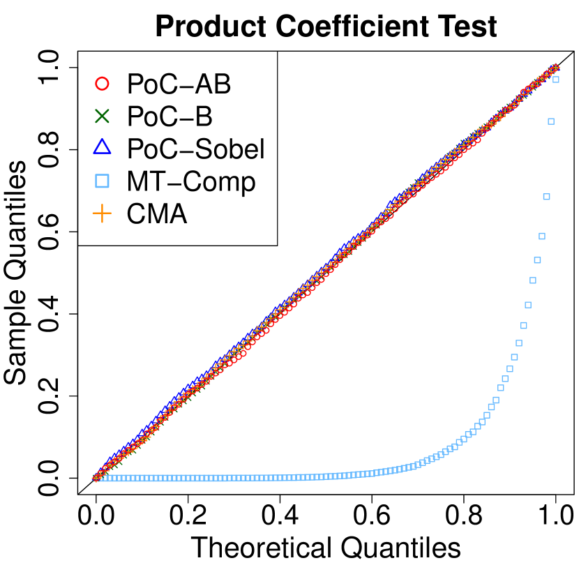
(a)    $H_{0,1}:(\alpha_{S},\beta_{M})=(0,0.5)$

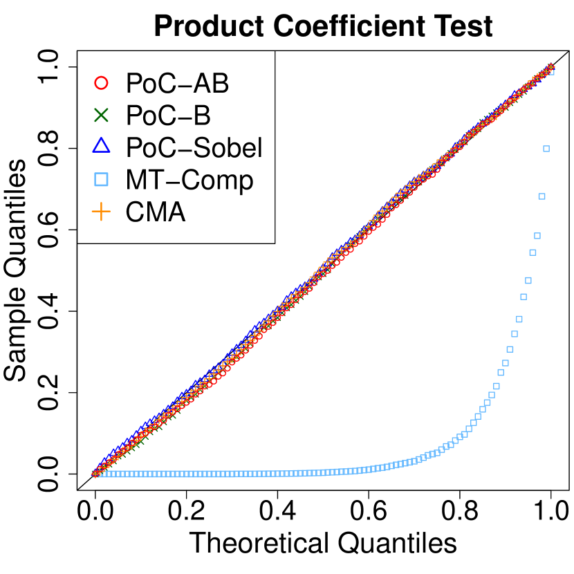
(b)    $H_{0,2}:(\alpha_{S},\beta_{M})=(0.5,0)$

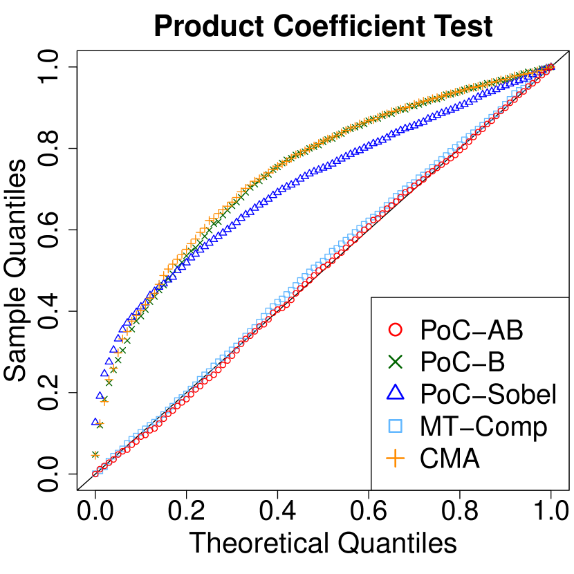
(c)    $H_{0,3}:(\alpha_{S},\beta_{M})=(0,0)$

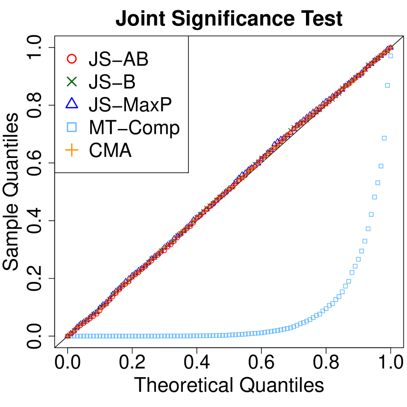
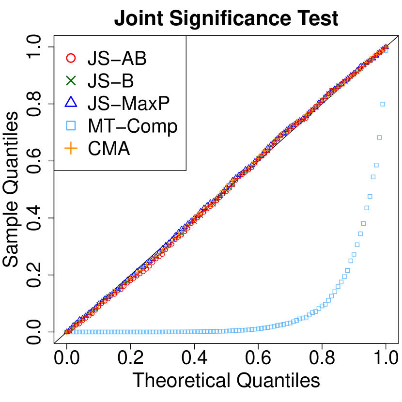
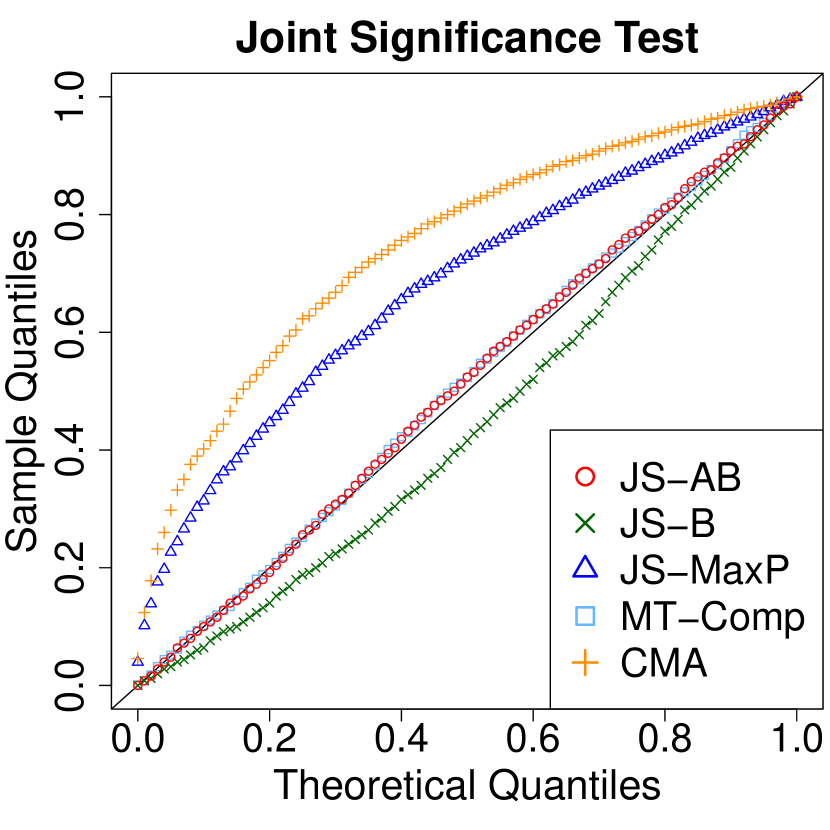
Figure 4 shows that for the PoC type of tests, under $H_{0,1}$ or $H_{0,2}$, the PoC-AB, the PoC-B, and the PoC-Sobel can correctly approximate the distribution of the PoC test statistic. However, under $H_{0,3}$, the PoC-B and the PoC-Sobel become conservative, while the proposed PoC-AB still approximates the distribution of the PoC statistic well. Similarly, for the JS type of tests, under $H_{0,1}$ or $H_{0,2}$, the JS-AB, the JS-B, and the JS-MaxP all work well. In contrast, under $H_{0,3}$, the JS-B inflates, and the JS-MaxP becomes conservative, while the JS-AB still exhibits a good performance. In addition, Figures 4 and 17 also display the results of both Huang (2019a)’s MT-Comp and the causal mediation analysis R package CMA (Tingley et al., 2014) for comparison. We observe that the MT-Comp properly controls the type I error under $H_{0,3}$, but fails to do so under $H_{0,2}$ and $H_{0,3}$ with inflated type I errors. This may be because the models considered in Huang (2019a) are not compatible with our simulation settings. On the other hand, the causal mediation R package (Tingley et al., 2014) produces uniformly distributed $p$-values under $H_{0,1}$ and $H_{0,2}$, but is conservative under $H_{0,3}$. This means that the R package CMA test is underpowered.

Setting 2: Under a random type of null.  In the second setting, we simulate data over 2000 Monte Carlo replications, where in each replication, the null hypothesis is not fixed but randomly selected from $H_{0,1}$–$H_{0,3}$ in (12). Specifically, for $(H_{0,1},H_{0,2},H_{0,3})$, we consider three selection probabilities (I) $(1/3,1/3,1/3)$, (II) $(0.2,0.2,0.6)$, and (III) $(0.05,0.05,0.9)$, respectively. We provide QQ-plots of $p$-values with $n=200$ in Figure 5, and QQ-plots under $n=500$ are similar and provided in Figure 18 of the Supplementary Material. In Figure 5, three subfigures in the first row present the results of the PoC tests with three null selection probabilities (I)–(III), respectively, and three subfigures in the second row present the corresponding results of the JS test, respectively.

Figures 5 shows that the adaptive bootstrap procedures for the PoC and JS tests perform well under different settings. The PoC-B test, PoC-Sobel’s test, the JS-MaxP test, and the R package CMA (Tingley et al., 2014) are conservative, and they become more conservative as the probability of choosing $H_{0,3}$ increases. We mention that in many biological studies such as genomics, $H_{0,3}$ predominates the null cases, hence these tests that are conservative under $H_{0,3}$ may not be preferred. Moreover, the JS-B test and the MT-Comp method can have inflated type I errors. The performance of JS-B becomes worse as the proportion of $H_{0,3}$ rises, while the MT-Comp method deteriorates as the proportions of $H_{0,1}$ and $H_{0,2}$ increase.

Figure 5: Q-Q plots of $p$-values under the mixture of nulls: $n=200$.

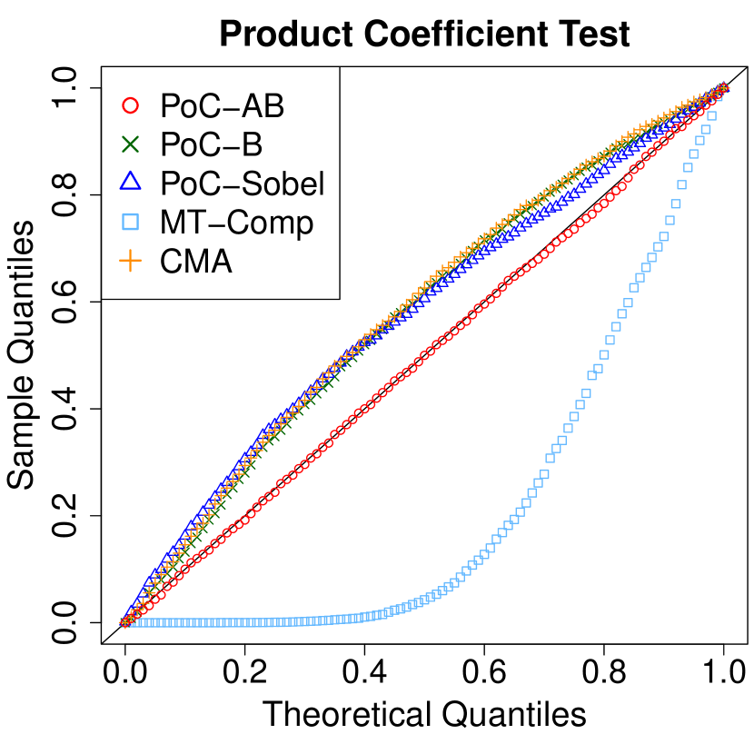
(a)    (I) $(1/3,1/3,1/3)$

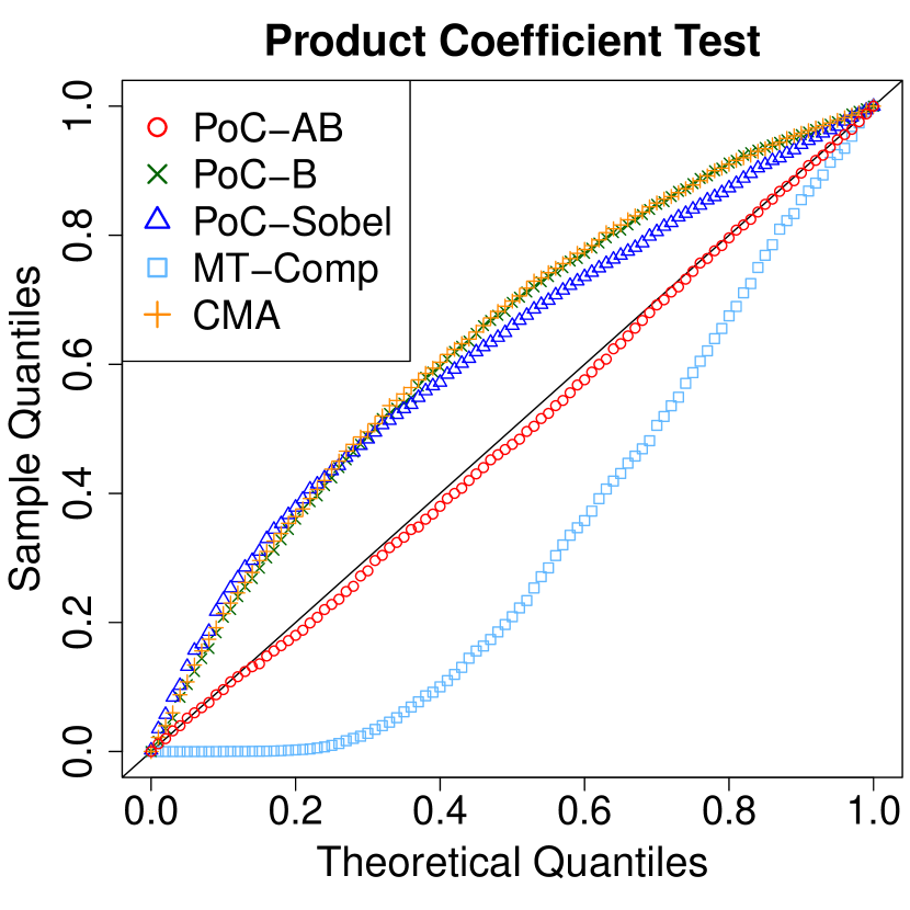
(b)    (II) $(0.2,0.2,0.6)$

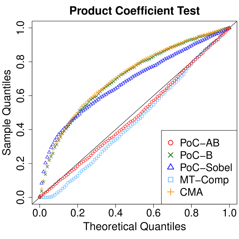
(c)    (III) $(0.05,0.05,0.9)$

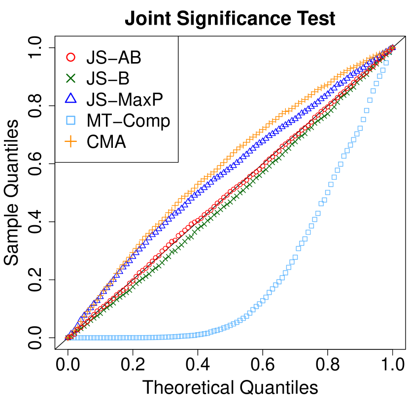
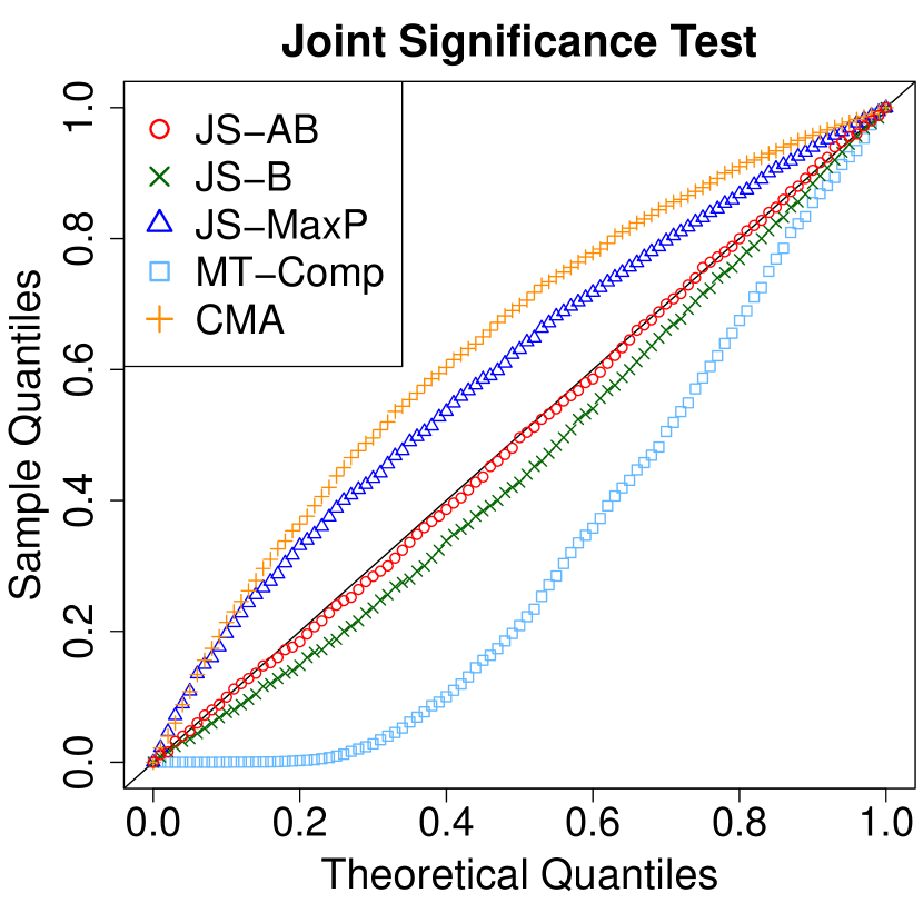
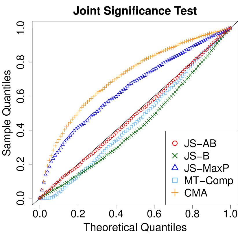
4.2 Alternative Hypotheses: Statistical Power

In this subsection, we evaluate the statistical power of the proposed AB tests under alternative hypotheses. Particularly, we simulate data under two settings: (I) fix $\alpha_{S}=\beta_{M}$ for the convenience of pictorial presentation, which takes various values beginning from zero; (II) fix the size of the mediation effect $\alpha_{S}\beta_{M}$, and vary the ratio $\alpha_{S}/\beta_{M}$. In the setting (I), we consider $n\in\{200,500\}$, and then plot the empirical rejection rates, based on 500 Monte Carlo replications, versus the signal size of $\alpha_{S}$, which is equal to $\beta_{M}$ in the setting (I). In the setting (II), we fix $\alpha_{S}\beta_{M}=0.04$ when $n=200$, and $\alpha_{S}\beta_{M}=0.015$ when $n=500$. Then we plot the empirical rejection rates versus the ratio $\alpha_{S}/\beta_{M}$. The results in the two settings (I) and (II) are shown in Figures 6 and 7, respectively.

Figures 6 and 7 show that for the three PoC tests, the PoC-AB has higher power than that of the classical nonparametric bootstrap, and both are more powerful than the Sobel’s test. Similarly, for the JS tests, the JS-AB has higher power than that of the classical bootstrap, and both have higher power than the MaxP test. In addition, the JS-B test has slightly inflated type I errors when $(\alpha_{S},\beta_{M})=(0,0)$, which is consistent with the results in Figure 4. Among the three classical methods (Sobel’s test, the MaxP test, and the PoC-B), the MaxP test seems to achieve the best balance between the type I error and the statistical power, while Sobel’s test has the lowest power. These findings are consistent with those reported in the current literature (MacKinnon et al., 2002; Barfield et al., 2017). Huang (2019a)’s MT-Comp test has shown seriously inflated type I errors in Figure 4, and therefore is not a fair competitor in our considered settings despite its high power. Overall, it is clear that the proposed PoC-AB and JS-AB tests are superior over these existing methods, with the most robust control of type I error and highest power.

Figure 6: Empirical rejection rates (power) versus the signal strength of $\alpha_{S}=\beta_{M}$.

Figure 7: Empirical rejection rates (power) versus the ratio $\alpha_{S}/\beta_{M}$.

5 Extensions

The adaptive bootstrap in Section 3 offers a general strategy that can be extended in a wide range of scenarios beyond the model (2). We next examine three examples, including testing the joint mediation effect of multivariate mediators in Section 5.1, testing the mediation effect in terms of odds ratio for a binary outcome in Section 5.2, and testing the mediation effect in terms of risk difference when the outcome is continuous, and the mediator follows a generalized linear model in Section 5.3. In each scenario, we present details in the order of (1) Model, (2) Non-regularity issue, (3) Asymptotic theory and adaptive bootstrap, and (4) Numerical results.

5.1 Testing Joint Mediation Effect of Multivariate Mediators

When the number of mediators is large, it can also be of interest to conduct group-based mediation analyses for a set of mediators (VanderWeele and Vansteelandt, 2014; Daniel et al., 2015; Huang and Pan, 2016; Sohn and Li, 2019; Hao and Song, 2022); also see a review in Blum et al. (2020). In this section, we show that the proposed AB method can be generalized to test joint mediation effects.

(1) Model. As an extension of (2), we consider the multivariate linear SEM (VanderWeele and Vansteelandt, 2014; Huang and Pan, 2016; Hao and Song, 2022),

$$M_{j}=\alpha_{S,j}S+\boldsymbol{X}^{\top}\alpha_{\boldsymbol{X},j}+\epsilon_{M,j},\hskip 20.00003ptY=\sum_{j=1}^{J}\beta_{M,j}M_{j}+\boldsymbol{X}^{\top}\boldsymbol{\beta}_{\boldsymbol{X}}+\tau_{S}S+\epsilon_{Y},$$ (13)

where $\boldsymbol{X}$ denotes a vector of confounders with the first element being 1 for the intercept, $\epsilon_{Y}$ and $\boldsymbol{\epsilon}_{M}:=(\epsilon_{M,1},\ldots,\epsilon_{M,J})^{\top}$ are independent error terms with mean zero, $\mathrm{var}(\epsilon_{Y})=\sigma_{\epsilon_{Y}}^{2}$, and $\mathrm{cov}(\boldsymbol{\epsilon}_{M})=\boldsymbol{\Sigma}_{M}$. Assume identification conditions similar to those in Section 2 (see Condition 3 in the Supplementary Material). The joint mediation effect through the group of mediators $\boldsymbol{M}$ is $\mathrm{E}\{Y(s,\boldsymbol{M}(s))-Y(s,\boldsymbol{M}(s^{*}))\}=(s-s^{*})\boldsymbol{\alpha}_{S}^{\top}\boldsymbol{\beta}_{M}$ (Huang and Pan, 2016), where $\boldsymbol{\alpha}_{S}=(\alpha_{S,1},\ldots,\alpha_{S,J})^{\top}$ and $\boldsymbol{\beta}_{M}=(\beta_{M,1},\ldots,\beta_{M,J})^{\top}$.

(2) Non-Regularity Issue. We are interested in $H_{0}:$ joint mediation effect $=0$, which is equivalent to $H_{0}:\boldsymbol{\alpha}_{S}^{\top}\boldsymbol{\beta}_{M}=0$. Similarly to Section 3, when $(\boldsymbol{\alpha}_{S},\boldsymbol{\beta}_{M})\neq\boldsymbol{0}$, i.e., there exists at least one coefficients $\alpha_{S,j}\neq 0$ or $\beta_{M,j}\neq 0$, we have ${\partial(\boldsymbol{\alpha}_{S}^{\top}\boldsymbol{\beta}_{M})}/{\partial\alpha_{S,j}}=\beta_{M,j}\neq 0$ or ${\partial(\boldsymbol{\alpha}_{S}^{\top}\boldsymbol{\beta}_{M})}/{\partial\beta_{M,j}}=\alpha_{S,j}\neq 0$. However, when $(\boldsymbol{\alpha}_{S},\boldsymbol{\beta}_{M})=\boldsymbol{0}$, i.e., $\alpha_{S,j}=\beta_{M,j}=0$ for all $j\in\{1,\ldots,J\}$, ${\partial(\boldsymbol{\alpha}_{S}^{\top}\boldsymbol{\beta}_{M})}/{\partial\alpha_{S,j}}={\partial(\boldsymbol{\alpha}_{S}^{\top}\boldsymbol{\beta}_{M})}/{\partial\beta_{M,j}}=0$ for all $j\in\{1,\ldots,J\}$. We expect that a non-regularity issue similar to that in Section 3 would occur when $(\boldsymbol{\alpha}_{S},\boldsymbol{\beta}_{M})=\boldsymbol{0}$. This issue is also illustrated by numerical experiments in Section D.2.4 of the Supplementary Material.

(3) Asymptotic Theory and Adaptive Bootstrap. To better understand the non-regularity issue, we similarly consider a local linear SEM $M_{j}=\alpha_{S,j,n}S+\boldsymbol{X}^{\top}\alpha_{\boldsymbol{X},j}+\epsilon_{M,j},$ and $Y=\sum_{j=1}^{J}\beta_{M,j,n}M_{j}+\boldsymbol{X}^{\top}\boldsymbol{\beta}_{\boldsymbol{X}}+\tau_{S}S+\epsilon_{Y}$, where ${\alpha}_{S,j,n}={\alpha}_{S,j}+n^{-1/2}{b}_{\alpha,j}$ and ${\beta}_{M,j,n}={\beta}_{M,j}+n^{-1/2}{b}_{\beta,j}$.

Theorem 3 (Asymptotic Property)

Under Conditions 3 and 4 (the latter is a regularity condition on the design matrix similar to Condition 1), and the local model,

• when $(\boldsymbol{\alpha}_{S},\boldsymbol{\beta}_{M})\neq\boldsymbol{0}$, $\sqrt{n}\times(\hat{\boldsymbol{\alpha}}_{S,n}^{\top}\hat{\boldsymbol{\beta}}_{M,n}-{\boldsymbol{\alpha}}_{S,n}^{\top}{\boldsymbol{\beta}}_{M,n})\xrightarrow{d}{\boldsymbol{\alpha}}_{S}^{\top}\vec{Z}_{M}+\boldsymbol{\beta}_{M}^{\top}\vec{Z}_{S};$

• when $(\boldsymbol{\alpha}_{S},\boldsymbol{\beta}_{M})=\boldsymbol{0}$, $n\times(\hat{\boldsymbol{\alpha}}_{S,n}^{\top}\hat{\boldsymbol{\beta}}_{M,n}-{\boldsymbol{\alpha}}_{S,n}^{\top}{\boldsymbol{\beta}}_{M,n})\xrightarrow{d}\boldsymbol{b}_{0,\alpha}^{\top}\vec{Z}_{M}+\boldsymbol{b}_{0,\beta}^{\top}\vec{Z}_{S}+\vec{Z}_{S}^{\top}\vec{Z}_{M},$

where $(\vec{Z}_{S},\vec{Z}_{M})$ are defined to be multivariate counterparts of $({Z}_{S},{Z}_{M})$ in Theorem 1, and the detailed definitions are given in Section D.2.2 of the Supplementary Material.

To present the theory of bootstrap consistency, we define the multivariate counterparts of ${\mathbb{R}}_{n}^{*}(b_{\alpha},b_{\beta})$ in Section 3 as $\vec{\mathbb{R}}_{n}^{*}(\boldsymbol{b}_{\alpha},\boldsymbol{b}_{\beta})$. The detailed forms are given in Section D.2.3 of the Supplementary Material. Similarly to $U^{*}$ in Section 3, we define the AB statistic under the multivariate setting as

$$\vec{U}^{*}=(\hat{\boldsymbol{\alpha}}_{S,n}^{*\top}\hat{\boldsymbol{\beta}}_{M,n}^{*}-\hat{\boldsymbol{\alpha}}_{S,n}^{\top}\hat{\boldsymbol{\beta}}_{M,n})\times(1-\vec{\mathrm{I}}_{\lambda_{n}}^{*})+n^{-1}\vec{\mathbb{R}}_{n}^{*}(\boldsymbol{b}_{\alpha},\boldsymbol{b}_{\beta})\times\vec{\mathrm{I}}_{\lambda_{n}}^{*},$$

where $\vec{\mathrm{I}}_{\lambda_{n}}^{*}=\mathrm{I}\{\,\max\{|T_{\alpha,j,n}|,\,|T_{\alpha,j,n}^{*}|,\,|T_{\beta,j,n}|,\,|T_{\beta,j,n}^{*}|:\,1\leqslant j\leqslant J\}\leqslant\lambda_{n}\,\},$ where $T_{\alpha,j,n}=\sqrt{n}\hat{\alpha}_{S,j}/\hat{\sigma}_{\alpha_{S},j,n}$ and $T_{\beta,j,n}=\sqrt{n}\hat{\beta}_{M,j,n}/\hat{\sigma}_{\beta_{M},j,n}$ denote the sample T-statistics of the two coefficients $\alpha_{S,j}$ and $\beta_{M,j}$, respectively, and $T_{\alpha,j,n}^{*}=\sqrt{n}\hat{\alpha}_{S,j}^{*}/\hat{\sigma}_{\alpha_{S},j,n}^{*}$ and $T_{\beta,j,n}^{*}=\sqrt{n}\hat{\beta}_{M,j,n}^{*}/\hat{\sigma}_{\beta_{M},j,n}^{*}$ denote the bootstrap counterparts of the two sample T-statistics. We establish bootstrap consistency for the joint AB statistic $\vec{U}^{*}$ below.

Theorem 4 (Adaptive Bootstrap Consistency)

Under the conditions of Theorem 3, when the tuning parameter $\lambda_{n}$ satisfies $\lambda_{n}=o(\sqrt{n})$ and $\lambda_{n}\to\infty$ as $n\to\infty,$

$$c_{n}\vec{U}^{*}\overset{d^{*}}{\leadsto}c_{n}(\hat{\boldsymbol{\alpha}}_{S,n}^{\top}\hat{\boldsymbol{\beta}}_{M,n}-{\boldsymbol{\alpha}}_{S,n}^{\top}{\boldsymbol{\beta}}_{M,n}),$$

where $c_{n}$ is specified as in (9).

Based on Theorem 4, we can develop an AB test similar to that in Section 3.

(4) Numerical Results. To evaluate the performance of the joint AB test, we conduct numerical experiments, detailed in Section D.2.4 of the Supplementary Material. We compare the AB test with the classical bootstrap and two tests in Huang and Pan (2016): the Product Test based on Normal Product distribution (PT-NP) and the Product Test based on Normality (PT-N). We observe results similar to those in Section 4. Specifically, under $H_{0}:\boldsymbol{\alpha}_{S}^{\top}\boldsymbol{\beta}_{M}=0$, when $(\boldsymbol{\alpha}_{S},\boldsymbol{\beta}_{M})\neq\mathbf{0}$, both the proposed AB test and the compared methods yield uniformly distributed $p$-values. However, when $(\boldsymbol{\alpha}_{S},\boldsymbol{\beta}_{M})=\mathbf{0}$, the compared methods become overly conservative, whereas the AB test still produces uniformly distributed $p$-values. Under $H_{A}$, the AB test can achieve higher empirical power than the compared methods. Besides simulations, we also provide an exemplary data analysis in Section G.3.2 of the Supplementary Material.

5.2 Non-Linear Scenario I: Binary Outcome and General Mediator

(1) Model. Suppose the outcome is binary, and consider the model

$$P(Y=1\mid S,M,\boldsymbol{X})= ~{}\mathrm{logit}^{-1}(\beta_{M}M+\boldsymbol{X}^{\top}\boldsymbol{\beta}_{\boldsymbol{X}}+\tau_{S}S),$$ (14)

$$\mathrm{E}(M\mid S,\boldsymbol{X})= ~{}h^{-1}(\alpha_{S}S+\boldsymbol{X}^{\top}\boldsymbol{\alpha}_{\boldsymbol{X}}),$$

where $h^{-1}(\cdot)$ is the inverse of a canonical link function in generalized linear models. Under Model (14), since the outcome is binary, it is conventional to define the mediation effect as the odds ratio (VanderWeele and Vansteelandt, 2010). Specifically, under the identification assumption given in Section 2, the conditional natural indirect effect (mediation effect) can be identified as

$$\mathrm{OR}^{\mathrm{NIE}}_{s\mid s^{*}}(s,\boldsymbol{x})=\frac{P\left\{Y(s,M(s))=1\mid\boldsymbol{X}=\boldsymbol{x}\right\}/\left\{1-P\left(Y(s,M(s))=1\mid\boldsymbol{X}=\boldsymbol{x}\right)\right\}}{P\left\{Y(s,M(s^{*}))=1\mid\boldsymbol{X}=\boldsymbol{x}\right\}/\left\{1-P\left\{Y(s,M(s^{*}))=1\mid\boldsymbol{X}=\boldsymbol{x}\right\}\right\}},$$

where $M(s)$ denotes the potential value of the mediator under the exposure $S=s$, and $Y(s,m)$ denotes the potential outcome that would have been observed if $S$ and $M$ had been set to $s$ and $m$, respectively. Under $H_{0}$ of no mediation effect,

$$H_{0}:\mathrm{OR}^{\mathrm{NIE}}_{s\mid s^{*}}(s,\boldsymbol{x})=1\ \Leftrightarrow\ ~{}\log\mathrm{OR}^{\mathrm{NIE}}_{s\mid s^{*}}(s,\boldsymbol{x})=0$$ (15)

$$\ \Leftrightarrow\ ~{}P\left\{Y(s,M(s))=1\mid\boldsymbol{X}=\boldsymbol{x}\right\}-P\left\{Y(s,M(s^{*}))=1\mid\boldsymbol{X}=\boldsymbol{x}\right\}=0,$$

where the second equivalence follows from the strict increasing monotonicity of the function $x/(1-x)$ when $0<x<1$.

Remark 4

We consider natural indirect/mediation effects conditioning on covariates $\boldsymbol{X}=\boldsymbol{x}$ following VanderWeele and Vansteelandt (2010). Alternatively, Imai et al. (2010a) proposed to examine the average NIE that marginalizes the distribution of $\boldsymbol{X}$. Examining the conditional NIE is mainly for technical convenience. The conditional NIE $=0$ for all $\boldsymbol{x}$ can give a sufficient condition for the average NIE $=0$. Conclusions of conditional NIE may be obtained for average NIE similarly. Please see Remark E.23 in the Supplementary Material for more details.

(2) Non-Regularity Issue. The null hypothesis of no mediation effect (15) looks different from $H_{0}:\alpha_{S}\beta_{M}=0$ under the linear SEMs in Section 2. Nevertheless, we can show that the non-regularity issue similar to that in Section 2 would still arise. This is formally stated as Proposition 5 below.

Proposition 5

Under the model (14), Condition 5 (a general regularity condition on the link function $h^{-1}(\cdot)$ and the distribution of $M$), and identification conditions in Section 2,

1. $H_{0}$ (15) holds for $s\neq s^{*}$ if and only if $\alpha_{S}=0$ or $\beta_{M}=0$.

2. For simplicity of notation, let $\mathrm{NIE}$ be a shorthand for $\log\mathrm{OR}^{\mathrm{NIE}}_{s\mid s^{*}}(s,\boldsymbol{x})$. We have
    (i) $\frac{\partial\mathrm{NIE}}{\partial\alpha_{S}}\Big{|}_{\beta_{M}=0}=\frac{\partial\mathrm{NIE}}{\partial\beta_{M}}\Big{|}_{\alpha_{S}=0}=0$,  (ii) $\frac{\partial\mathrm{NIE}}{\partial\alpha_{S}}\Big{|}_{\alpha_{S}=0,\beta_{M}\neq 0}\neq 0$,  (iii) $\frac{\partial\mathrm{NIE}}{\partial\beta_{M}}\Big{|}_{\alpha_{S}\neq 0,\beta_{M}=0}\neq 0$.

It is interesting to see that even though the conditional mediation effect $\mathrm{OR}^{\mathrm{NIE}}_{s\mid s^{*}}(s,\boldsymbol{x})$ does not take a product form, a non-regularity issue caused by zero gradient can still arise under $H_{0}$ in (15), which is similar to the PoC statistic in Section 3. Specifically, Proposition 5 implies that when $\alpha_{S}=\beta_{M}=0$, the first-order Delta method cannot be directly applied to the inference of $\mathrm{NIE}$, which is different from the scenarios when $\alpha_{S}\neq 0$ or $\beta_{M}\neq 0$. Therefore, we expect that the ordinary estimator of NIE can behave differently under different types of null hypotheses, and a non-regularity issue can occur. This phenomenon is indeed demonstrated by numerical experiments in Section E.2 of the Supplementary Material.

(3) Asymptotic Theory and Adaptive Bootstrap. For ease of presentation, we next derive asymptotic theory under a special case of (14), where the mediator is binary and follows a logistic regression model. We point out that the analysis in this section can be readily extended to cases where the mediator $M$ follows a linear model or other canonical generalized linear models. Specifically, let $M$ and $Y$ be Bernoulli random variables with mean values in (14), and $h^{-1}(x)=\mathrm{logit}^{-1}(x)$. In this case, $\log\mathrm{OR}^{\text{NIE}}_{s\mid s^{*}}(s,\boldsymbol{x})=l(P_{s})-l(P_{s^{*}}),$ where $P_{s}:=P\left\{Y(s,M(s))=1\mid\boldsymbol{X}=\boldsymbol{x}\right\}$, $P_{s^{*}}:=P\left\{Y(s,M(s^{*}))=1\mid\boldsymbol{X}=\boldsymbol{x}\right\},$ and $l(x)=\log\frac{x}{1-x}$. Similarly to Section 3, we are interested in understanding how the local limiting behaviors of $\alpha_{S}$ and $\beta_{M}$ coefficients change. To this end, we consider a general local logistic model:

$$\mathrm{E}(M\mid S,\boldsymbol{X})=g(\alpha_{S,n}S+\boldsymbol{X}^{\top}\boldsymbol{\alpha}_{\boldsymbol{X}}),\hskip 15.00002pt\mathrm{E}(Y\mid S,M,\boldsymbol{X})=g(\beta_{M,n}M+\boldsymbol{X}^{\top}\boldsymbol{\beta}_{\boldsymbol{X}}+\tau_{S}S),$$ (16)

where $\alpha_{S,n}=\alpha_{S}+b_{\alpha}/\sqrt{n}$, $\beta_{M,n}=\beta_{M}+b_{\beta}/\sqrt{n}$, and $g(x)=\mathrm{logit}^{-1}(x)=e^{x}/(1+e^{x})$. Under the local model (16), we have for $\iota\in\{s,s^{*}\}$,

$$P_{\iota}= ~{}g\big{(}\iota\times\alpha_{S,n}+\boldsymbol{x}^{\top}\boldsymbol{\alpha}_{\boldsymbol{X}}\big{)}\times d_{\beta,n}+P_{*},$$ (17)

where $d_{\beta,n}=g(\beta_{M,n}+\boldsymbol{x}^{\top}\boldsymbol{\beta}_{\boldsymbol{X}}+\tau_{S}s)-g(\boldsymbol{x}^{\top}\boldsymbol{\beta}_{\boldsymbol{X}}+\tau_{S}s)$ and $P_{*}=g(\boldsymbol{x}^{\top}\boldsymbol{\beta}_{\boldsymbol{X}}+\tau_{S}s)$. (Please see the proof of Theorem 6 for the derivations.) For simplicity of notation, let NIE be a shorthand of $\log\mathrm{OR}^{\text{NIE}}_{s\mid s^{*}}(s,\boldsymbol{x})$, and by (15), $H_{0}\Leftrightarrow$ NIE $=0$. Let $\widehat{\text{NIE}}=l(\hat{P}_{s})-l(\hat{P}_{s^{*}})$ denote an estimator of NIE, where $\hat{P}_{s}$ and $\hat{P}_{s^{*}}$ are defined similarly to (17) with $({\alpha}_{S,n},{\boldsymbol{\alpha}}_{\boldsymbol{X}},{\beta}_{M,n},{\boldsymbol{\beta}}_{\boldsymbol{X}},{\tau}_{S})$ replaced by their corresponding sample regression coefficient estimators $(\hat{\alpha}_{S},\hat{\boldsymbol{\alpha}}_{\boldsymbol{X}},\hat{\beta}_{M},\hat{\boldsymbol{\beta}}_{\boldsymbol{X}},\hat{\tau}_{S})$.

Theorem 6 (Asymptotic Property)

Assume $P_{s}$ and $P_{s^{*}}\in(0,1)$ and Condition 6 in the Supplementary Material (a regularity condition on the design matrix similar to Condition 1). Under the local model (16) and $H_{0}:$ $\alpha_{S}\beta_{M}=0$,

• when $(\alpha_{S},\beta_{M})\neq\mathbf{0}$, $\sqrt{n}(\widehat{\mathrm{NIE}}-\mathrm{NIE})\xrightarrow{d}(d_{\alpha}Z_{\beta}+d_{\beta}Z_{\alpha})\gamma_{0};$

• when $(\alpha_{S},\beta_{M})=\mathbf{0}$, $n(\widehat{\mathrm{NIE}}-\mathrm{NIE})\xrightarrow{d}(d_{b_{\alpha}}Z_{\beta}+d_{b_{\beta}}Z_{\alpha}+Z_{\alpha}Z_{\beta})\gamma_{0},$

where $d_{\alpha}=g(\alpha_{S}s+\boldsymbol{x}^{\top}\boldsymbol{\alpha}_{\boldsymbol{X}})-g(\alpha_{S,n}s^{*}+\boldsymbol{x}^{\top}\boldsymbol{\alpha}_{\boldsymbol{X}})$, $d_{\beta}=g(\beta_{M}+\boldsymbol{x}^{\top}\boldsymbol{\beta}_{\boldsymbol{X}}+\tau_{S}s)-g(\boldsymbol{x}^{\top}\boldsymbol{\beta}_{\boldsymbol{X}}+\tau_{S}s)$, $d_{b_{\alpha}}=g^{\prime}(\boldsymbol{x}^{\top}\boldsymbol{\alpha}_{\boldsymbol{X}})(s-s^{*})b_{\alpha}$, $d_{b_{\beta}}=g^{\prime}(\boldsymbol{x}^{\top}\boldsymbol{\beta}_{\boldsymbol{X}}+\tau_{S}s)(s-s^{*})b_{\beta}$, $(Z_{\alpha},Z_{\beta})$ represent bivariate mean-zero normal distributions specified in Lemma E.24, and $\gamma_{0}=\{P_{*}(1-P_{*})\}^{-1}$ is a non-zero constant with $P_{*}$ given in (17).

We next study consistency of bootstrap estimators. Let $\widehat{\mathrm{NIE}}^{*}$ denote the classical nonparametric bootstrap estimator of $\mathrm{NIE}$. Specifically, $\widehat{\mathrm{NIE}}^{*}=l(\hat{P}_{s}^{*})-l(\hat{P}_{s^{*}}^{*})$, where $\hat{P}_{s}^{*}$, and $\hat{P}_{s^{*}}^{*}$ are defined similarly to (17) with $({\alpha}_{S,n},{\boldsymbol{\alpha}}_{\boldsymbol{X}},{\beta}_{M,n},{\boldsymbol{\beta}}_{\boldsymbol{X}},{\tau}_{S})$ replaced by their classical nonparametric bootstrap estimators $(\hat{\alpha}_{S}^{*},\hat{\boldsymbol{\alpha}}_{\boldsymbol{X}}^{*},\hat{\beta}_{M}^{*},\hat{\boldsymbol{\beta}}_{\boldsymbol{X}}^{*},\hat{\tau}_{S}^{*}).$ Motivated by Theorem 6, we define the AB statistic

$$U_{e,1}^{*}=(\widehat{\mathrm{NIE}}^{*}-\widehat{\mathrm{NIE}})\times(1-\mathrm{I}_{\alpha_{S},\lambda_{n}}^{*}\mathrm{I}_{\beta_{M},\lambda_{n}}^{*})+n^{-1}\big{(}d_{b_{\alpha}}\mathbb{Z}_{\beta}^{*}+d_{b_{\beta}}\mathbb{Z}_{\alpha}^{*}+\mathbb{Z}_{\alpha}\mathbb{Z}_{\beta}^{*}\big{)}\hat{\gamma}_{0}^{*}\times\mathrm{I}_{\alpha_{S},\lambda_{n}}^{*}\mathrm{I}_{\beta_{M},\lambda_{n}}^{*},$$

where $\mathrm{I}_{\alpha_{S},\lambda_{n}}^{*}$ and $\mathrm{I}_{\beta_{M},\lambda_{n}}^{*}$ are defined similarly to (8). The following theorem proves consistency of the AB statistic $U_{e,1}^{*}$, based on which we can develop an AB test similar to that in Section 3.

Theorem 7 (Adaptive Bootstrap Consistency)

Under the conditions of Theorem 6, when the tuning parameter $\lambda_{n}$ satisfies $\lambda_{n}=o(\sqrt{n})$ and $\lambda_{n}\to\infty$ as $n\to\infty,$ $c_{n}U_{e,1}^{*}\overset{d^{*}}{\leadsto}c_{n}(\widehat{\mathrm{NIE}}-\mathrm{NIE}),$ where $c_{n}$ is specified as in (9).

(4) Numerical Results. We conduct simulation studies to compare the AB and the classical non-parametric bootstrap under the model (14). The detailed results are provided in Section E.2 of the Supplementary Material. Our findings align closely with those presented in Section 4. Specifically, under $H_{0}:{\alpha}_{S}{\beta}_{M}=0$, when $({\alpha}_{S},{\beta}_{M})\neq\mathbf{0}$, both the proposed AB test and the classical non-parametric bootstrap yield uniformly distributed $p$-values. However, when $({\alpha}_{S},{\beta}_{M})=\mathbf{0}$, the classical bootstrap becomes overly conservative, whereas the AB test still yields uniformly distributed $p$-values. Under $H_{A}$, the AB test can achieve higher empirical power than the classical bootstrap.

5.3 Non-Linear Scenario II: Linear Outcome and General Mediator

(1) Model. Suppose the outcome follows a linear model, and consider

$$\mathrm{E}(M\mid S,\boldsymbol{X})=h^{-1}(\alpha_{S}S+\boldsymbol{X}^{\top}\boldsymbol{\alpha}_{\boldsymbol{X}}),\hskip 15.00002pt\mathrm{E}(Y\mid S,M,\boldsymbol{X})=\beta_{M}M+\boldsymbol{X}^{\top}\boldsymbol{\beta}_{\boldsymbol{X}}+\tau_{S}S,$$ (18)

where $h^{-1}(\cdot)$ can be the inverse of a canonical link function. Similarly to the non-linear Scenario I, we examine the conditional natural indirect effect/mediation effect defined as the risk difference:

$$\mathrm{NIE}_{s\mid s^{*}}(s,\boldsymbol{x}):= ~{}\mathrm{E}\big{\{}Y(s,M(s))-Y(s,M(s^{*}))\mid\boldsymbol{X}=\boldsymbol{x}\big{\}}$$

$$= ~{}\beta_{M}\left\{h^{-1}\big{(}\alpha_{S}s+\boldsymbol{x}^{\top}\boldsymbol{\alpha}_{\boldsymbol{X}}\big{)}-h^{-1}\big{(}\alpha_{S}s^{*}+\boldsymbol{x}^{\top}\boldsymbol{\alpha}_{\boldsymbol{X}}\big{)}\right\}.$$ (19)

(2) Non-Regularity Issue. We are interested in testing $H_{0}:\mathrm{NIE}_{s\mid s^{*}}(s,\boldsymbol{x})=0$, which looks different from $H_{0}:\alpha_{S}\beta_{M}=0$ in Section 2. Nevertheless, we can show that the non-regularity issue similar to that in Section 2 would arise. This is formally stated as Proposition 8 below.

Proposition 8

Under the model (18), assume $h^{-1}(\cdot)$ is strictly monotone, and the identification conditions in Section 2 hold. Let $\mathrm{NIE}$ be a shorthand for $\mathrm{NIE}_{s\mid s^{*}}(s,\boldsymbol{x})$ in (19). Then

1. $H_{0}:$ $\mathrm{NIE}=\eqref{eq:h0binarymediator}=0$ holds if and only if $\alpha_{S}=0$ or $\beta_{M}=0$.

2. (i) $\frac{\partial\mathrm{NIE}}{\partial\alpha_{S}}\Big{|}_{\beta_{M}=0}=\frac{\partial\mathrm{NIE}}{\partial\beta_{M}}\Big{|}_{\alpha_{S}=0}=0$.  (ii) $\frac{\partial\mathrm{NIE}}{\partial\alpha_{S}}\Big{|}_{\alpha_{S}=0,\beta_{M}\neq 0}\neq 0$.  (iii) $\frac{\partial\mathrm{NIE}}{\partial\beta_{M}}\Big{|}_{\alpha_{S}\neq 0,\beta_{M}=0}\neq 0$.

Similarly to Proposition 5, Proposition 8 implies that a non-regularity issue caused by zero gradient would arise under $H_{0}$. Specifically, the ordinary estimator of NIE can behave differently when $\alpha_{S}=\beta_{M}=0$, and when one of $\alpha_{S}$ and $\beta_{M}\neq 0$. This is similar to the PoC statistic in Section 3 and the odds ratio in Section 5.2.

(3) Asymptotic Theory and Adaptive Bootstrap. For ease of presentation, we next derive asymptotic theory under a specific instance of (18). Specifically, the mediator $M$ is a Bernoulli random variable with its conditional mean given in (14) and $h^{-1}(x)=\mathrm{logit}^{-1}(x)=e^{x}/(1+e^{x})$, and the outcome $Y$ follows the linear model in (2). The analysis in this section can be readily extended when the mediator $M$ follows other canonical generalized linear models. As we are interested in how the local limiting behavior of $\alpha_{S}$ and $\beta_{M}$ coefficients change, we consider the following general local model

$$\mathrm{E}(M\mid S,\boldsymbol{X})=\mathrm{logit}^{-1}(\alpha_{S,n}S+\boldsymbol{X}^{\top}\boldsymbol{\alpha}_{\boldsymbol{X}}),\hskip 20.00003ptY=\beta_{M,n}M+\boldsymbol{X}^{\top}\boldsymbol{\beta}_{\boldsymbol{X}}+\tau_{S}S+\epsilon_{Y}.$$ (20)

where $\alpha_{S,n}=\alpha_{S}+b_{\alpha}/\sqrt{n}$, and $\beta_{M,n}=\beta_{M}+b_{\beta}/\sqrt{n}$.

Theorem 9 (Asymptotic Property)

Assume Condition 7 in the Supplementary Material (a regularity condition on the design matrix similar to Condition 1). Under model (20),

• when $(\alpha_{S},\beta_{M})\neq\mathbf{0}$, $\sqrt{n}(\widehat{\mathrm{NIE}}-\mathrm{NIE})\xrightarrow{d}d_{\alpha}Z_{\beta}+\beta_{M}Z_{\alpha}$;

• when $(\alpha_{S},\beta_{M})=\mathbf{0}$, $n(\widehat{\mathrm{NIE}}-\mathrm{NIE})\xrightarrow{d}d_{b_{\alpha}}Z_{\beta}+b_{\beta}Z_{\alpha}+Z_{\alpha}Z_{\beta}$,

where $d_{\alpha_{S}}=g(\alpha_{S}s+\boldsymbol{x}^{\top}\boldsymbol{\alpha}_{\boldsymbol{X}})-g(\alpha_{S,n}s^{*}+\boldsymbol{x}^{\top}\boldsymbol{\alpha}_{\boldsymbol{X}})$, $d_{b_{\alpha}}=g^{\prime}(\boldsymbol{x}^{\top}\boldsymbol{\alpha}_{\boldsymbol{X}})(s-s^{*})b_{\alpha}$, $Z_{\alpha}$ represents a normal distribution specified in Lemma E.24, and $Z_{\beta}$ is redefined to be a mean-zero normal distribution with a covariance same as the random vector $V_{M}^{-1}\epsilon_{Y}M_{\perp^{\prime}}$, where $V_{M}$ and $M_{\perp^{\prime}}$ are defined in Theorem 1.

We next establish bootstrap consistency theory. Similarly to Section 5.2, let $\widehat{\mathrm{NIE}}^{*}$ denote the nonparametric bootstrap estimator of $\mathrm{NIE}$. In particular, we redefine $\widehat{\mathrm{NIE}}^{*}=\hat{\beta}_{M}^{*}\{g(\hat{\alpha}_{S}^{*}s+\boldsymbol{x}^{\top}\hat{\boldsymbol{\alpha}}_{\boldsymbol{X}}^{*})-g(\hat{\alpha}_{S}^{*}s^{*}+\boldsymbol{x}^{\top}\hat{\boldsymbol{\alpha}}_{\boldsymbol{X}}^{*})\}$, where $(\hat{\alpha}_{S}^{*},\hat{\boldsymbol{\alpha}}_{\boldsymbol{X}}^{*},\hat{\beta}_{M}^{*})$ denotes the classical nonparametric bootstrap estimators of $({\alpha}_{S},{\boldsymbol{\alpha}}_{\boldsymbol{X}},{\beta}_{M})$. Motivated by Theorem 9, we define the AB statistic

$$U_{e,2}^{*}=(\widehat{\mathrm{NIE}}^{*}-\widehat{\mathrm{NIE}})(1-\mathrm{I}_{\alpha_{S},\lambda_{n}}^{*}\mathrm{I}_{\beta_{M},\lambda_{n}}^{*})+n^{-1}(d_{b_{\alpha}}\mathbb{Z}_{\beta}^{*}+b_{\beta}\mathbb{Z}_{\alpha}^{*}+\mathbb{Z}_{\alpha}^{*}\mathbb{Z}_{\beta}^{*})\mathrm{I}_{\alpha_{S},\lambda_{n}}^{*}\mathrm{I}_{\beta_{M},\lambda_{n}}^{*},$$

where $\mathrm{I}_{\alpha_{S},\lambda_{n}}^{*}$ and $\mathrm{I}_{\beta_{M},\lambda_{n}}^{*}$ are defined similarly to (8). The following theorem establishes consistency of the AB statistic $U_{e,2}^{*}$.

Theorem 10 (Adaptive Bootstrap Consistency)

Under conditions of Theorem 9, when the tuning parameter $\lambda_{n}$ satisfies $\lambda_{n}=o(\sqrt{n})$ and $\lambda_{n}\to\infty$ as $n\to\infty,$ $c_{n}U_{e,2}^{*}\overset{d^{*}}{\leadsto}c_{n}(\widehat{\mathrm{NIE}}-\mathrm{NIE}),$ where $c_{n}$ is specified as in (9).

(4) Numerical Results. We conduct simulation studies to compare the AB and the classical non-parametric bootstrap under the model (18). The detailed results are provided in Section E.2 of the Supplementary Material. The obtained results are very similar to those in Section 4 and Section 5.2 Part 4), and therefore, we refrain from repeating the details here.

6 Data Analysis

We illustrate an application of our proposed method to the analysis of data from a cohort study “Early Life Exposures in Mexico to ENvironmental Toxicants” (ELEMENT) (Perng et al., 2019). One of the central interests in this scientific study concerns the mediation effects of metabolites, in particular, the family of lipids, on the association between environmental exposure and children growth and development. In the literature of environmental health sciences, exposure to endocrine-disrupting chemicals (EDCs) such as phthalates have been found to be detrimental to children’s health outcomes. Such findings of direct associations need to be further assessed for possible mediation effects through metabolites, because environmental toxicants such as phthalates can alter metabolic profiles at the molecular level.

Our illustration focuses on the outcome of body mass index (BMI) and exposure to one phthalate, MEOHP (a chemical in food production and storage). BMI is a widely used biomarker in pediatric research to measure childhood obesity. The dataset contains 382 adolescents aged 10-18 years old living in Mexico City. Our mediation analysis involves a set of 149 lipids that are hypothesized to have potential mediation effects on children’s growth and development. Our goal is to identify the mediation pathways of exposure to MEOHP $\rightarrow$ lipids $\rightarrow$ BMI. Two key potential confounders, gender and age, are included throughout the analyses. It is worth noting that adjusting for gender and age may not be sufficient for proper confounding adjustments. To conduct a more plausible causal analysis and interpretation, a further investigation is deemed necessary to rigorously assess the underlying causal assumptions such as a sensitivity analysis for the sequential ignorability assumption. In our analyses, we compare the results of six tests: JS-AB, JS-MaxP, PoC-AB, PoC-B, PoC-Sobel, and CMA, which have been compared in our simulation studies in Section 4. In particular, all the bootstrap methods (including JS-AB, PoC-AB, PoC-B, CMA) are conducted based on $10^{4}$ bootstrap resamples. Here we no longer include the JS-B test and the MT-Comp method, as they are known to have inflated type I errors according to our simulation studies in Section 4.

As the sample size is limited compared to the large number of mediators, we first apply a screening analysis to identify a subset of lipids as potential candidates. We then jointly model the chosen lipids in the second step of our analysis. To mitigate the potential issues arising from double dipping the data, we adopt a random data splitting approach by dividing the dataset into two distinct parts, each dedicated to one of the two respective analytic tasks. In the first screening step, we examine the effect along the path MEOHP $\to$ lipid $\to$ BMI for one lipid at a time, and the corresponding $p$-values are obtained with the six tests, respectively. For each test, we select a proportion ($q\%$) of lipids with the smallest $p$-values. The second step examines the path MEOHP $\to$ selected lipids $\to$ BMI, with the selected lipids being modeled jointly. To test the mediation effect through a target lipid $M$ within the selected set, we adjust for non-target mediators within the outcome model, following the discussions on Page 3; please see more details in Section G.3.3 of the Supplementary Material. Subsequently, we select lipids based on their $p$-values obtained in the second step, after adjusting for multiple comparisons with controlled false discovery rate (FDR) (Benjamini and Hochberg, 1995). In our analysis, we explore a range of $q$ values $\{5,10,15,20,25\}$ and observe very similar results, indicating the robustness of our approach to the choice of the screening threshold in the first step. We next present the results obtained with $q=10$ (i.e., 15 selected lipids based on their $p$-values), while results for other $q$ values are detailed in Section G.3.1 of the Supplementary Material.

As an illustrative example, we first present the results from a single random split in Table 1. Table 1 provides the corresponding $p$-values for the lipids selected by at least one test in the second step of the analysis. In this instance, the non-AB tests fail to detect any lipids. In contrast, the PoC-AB test identifies lauric acid (L.A) and FA.7.0-OH_1 (FA.7) while controlling the FDR at 0.10, and the JS-AB test selects both L.A and FA.7 when the FDR is controlled at 0.05 and 0.10, respectively. To gauge the variability of results across random splits, we repeat the data-splitting analysis 400 times. As shown in Figure 8, L.A and FA.7 are the two most frequently selected mediators in our analysis. Furthermore, the AB tests exhibit a notably higher chance of selecting L.A compared to the non-AB tests. This aligns with our observations from simulations in Section 4, suggesting that the AB tests can attain higher power than their non-AB counterparts. Lauric acid is a saturated fatty acid and is found in many vegetable fats and in coconut and palm kernel oils (Dayrit, 2015). The results suggest that the exposure to MEOHP may influence the process of breaking down fat tissue in the human body, leading to obesity and other adverse health outcomes.

Table 1: Lipids selected in the second step.

Lipids	JS-AB	JS-MaxP	PoC-AB	PoC-B	PoC-Sobel	CMA
L.A	0.0017 ($\times*$)	0.0399	0.0043 ($*$)	0.0406	0.1254	0.0426
FA.7	0.0008 ($\times*$)	0.0146	0.0090 $(*)$	0.0236	0.0937	0.0208

• (Abbreviations: LAURIC.ACID (L.A); FA.7.0-OH_1 (FA.7). $p$-values with $(\times)$ and $(*)$ indicate that the lipid specified by the row is selected by the method specified by the column under 0.05 and 0.10 FDR levels, respectively.)
  

Since the first screening step considers one mediator at a time, we also conduct sensitivity analyses to evaluate the effects of the unadjusted mediators similarly to Liu et al. (2021). We use the procedure proposed by Imai et al. (2010b), which utilized the idea that the error term in the M-S model and that in the Y-M model are likely to be correlated if the sequential ignorability assumption is violated and vice versa. The detailed results are provided in Section G.3.4 in the Supplementary Material. As a brief summary, the sensitivity analysis suggests that our first screening analysis could be robust to unadjusted mediators.

(a) JS-AB

(b) JS-MaxP

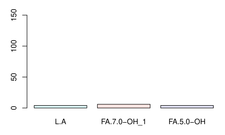
(c) CMA

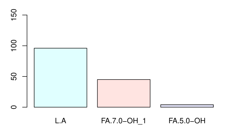
(d) PoC-AB

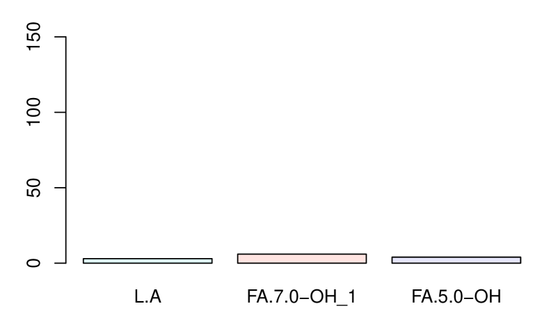
(e) PoC-B

(f) PoC-Sobel

Figure 8: Times of mediators being selected in Step 2 by the six tests with FDR$=0.10$ over 400 random splits of the data.

7 Discussion

This paper proposes a new adaptive framework for testing composite null hypotheses in mediation pathway analysis. The method incorporates a consistent pre-test threshold into the bootstrap procedure, which helps circumvent the non-regularity issue arising from the composite null hypotheses. If at least one of the two coefficients is significant, the procedure would reduce to the classical nonparametric bootstrap; otherwise, it approximates the local asymptotic behavior of the statistics. Our proposed strategy accommodates different types of null hypotheses under various models. Particularly, we have established similar results for both the individual and joint mediation effects under classical linear structural equation models, and we have generalized the conclusions under generalized linear models. Through comprehensive simulation studies, we have demonstrated that the adaptive tests can properly and robustly control the type I error under different types of null hypotheses and improve the statistical power.

The proposed methodology offers an exemplary analytic toolbox that can be broadly extended to handle other problems of similar types involving composite null hypotheses. There are several interesting future research directions that are worth exploration. First, the non-regularity issue can similarly arise in other scenarios, such as survival analysis (VanderWeele, 2011; Huang and Pan, 2016), different data types (Sohn and Li, 2019), partially linear models (Hines et al., 2021), and models with exposure-mediator interactions; see more discussions in Section H of the Supplementary Material. These complicated models require special care in the causal interpretation of mediation effects and in the implementation of the bootstrap procedure, warranting further investigation. Second, when the dimension of mediators and covariates becomes high, it is of interest to extend the adaptive bootstrap under high-dimensional mediation models for both individual and joint mediation effects (Zhou et al., 2020). Similarly to our discussions on adjusting multivariate mediators at the end of Section 3, we might apply the adaptive bootstrap after properly adjusting high-dimensional covariates. In the data analysis, we have applied the marginal screening to reduce the dimension of mediators, which might potentially overlook the complicated causal dependence among mediators. When mediators have potential causal dependence, Shi and Li (2022) proposed to first estimate a directed acyclic graph of mediators and develop a testing procedure that can control the type I error to be less than or equal to the nominal level. It would be of interest to extend our proposed AB under such settings to mitigate potential conservatism. Third, the proposed AB strategy can also be utilized to examine the replicability across independent studies (Bogomolov and Heller, 2018), which is fundamental to scientific discovery. Specifically, let $\beta_{i},i=1,\ldots,K$, denote the true signals from $K$ independent studies, respectively. Testing whether the signals in these $K$ studies are all significant corresponds to $H_{0}:\prod_{i=1}^{K}\beta_{i}=0$ versus $H_{A}:\prod_{i=1}^{K}\beta_{i}\neq 0$. Moreover, for two studies with true signals $\beta_{1}$ and $\beta_{2}$, to investigate whether the effects of both studies are significant in the same direction, one can formulate the hypothesis testing problem as $H_{0}:\beta_{1}\beta_{2}\leq 0$ versus $H_{A}:\beta_{1}\beta_{2}>0$. For these testing problems, the null hypotheses are composite. To properly control the type I error, the adaptive strategy proposed in this paper may serve as a valuable building block, while additional effort is needed to analyze those different cases carefully. Last, in our data analysis, all measurements are obtained cross-sectionally at one given clinical visit within a time window of approximately three months. To further study potential long-term influences of toxicant exposures, it may be of interest to investigate how the mediation effects might vary over time. Such time-varying mediation effects may be naturally analyzed in the scenario of longitudinal studies that collect time-varying measurements. This is a very challenging research field with only minimal investigation in the current literature (Bind et al., 2016). Extending the proposed AB method to analyze time-varying mediation effects would be a compelling future direction.

Supplementary Material

We provide more results in the online Supplementary Material, including all the proofs, hyperparameter tuning, additional results on simulations and data analysis, and details of extensions (Joint Significance test, multiple-mediator settings, and non-linear models). For reproducibility of our results, we provide the R package and code on the GitHub repository: He et al. (2023).

Data Availability

Due to privacy restrictions, we are unable to directly share the raw data publicly but they may be obtained offline according to a formal data request procedure outlined in the University of Michigan Data Use Agreement protocol. To satisfy the need of reproducibility, instead, we have introduced a pseudo-dataset with added noise on the GitHub repository: He et al. (2023).

Supplementary Material for
“Adaptive Bootstrap Tests for Composite Null Hypotheses in the Mediation Pathway Analysis”

In this Supplementary Material, Section A provides rigorous definitions of notation used in the main text and proofs. Section B presents details of the Adaptive Bootstrap for the Joint Significance Test, mentioned on Page 3 of the main text. Section C provides proofs of Theorems 1–2 and Theorems 11–12. Section D provides detailed theoretical and numerical results on multiple mediators supplementary to Figure 3 and Section 5 in the main text. Section E provides detailed theoretical and numerical results on non-linear models supplementary to Sections 5.2 and 5.3. Section F discuss implementation details of a data-driven procedure for choosing the tuning parameter. Section G provides additional numerical experiments and data analysis results. Section H provides a clarification of the partially linear model mentioned in Section 7 of the main text.

Appendix A Definitions and Notation

Notation on Convergence

For two sequences of real numbers $\{a_{n}\}$ and $\{b_{n}\}$, we write $a_{n}=o(b_{n})$ if $\lim_{n\to\infty}a_{n}/b_{n}=0$. We say $a_{n}\to\infty$ as $n\to\infty$ if the value of $a_{n}$ can be arbitrarily large by taking $n$ to be sufficiently large. Given a sequence of random variables $\{X_{n}\}$ and a random variable $X$, we let $X_{n}\xrightarrow{\mathrm{P}}X$ represent the convergence in probability, i.e., for any $\epsilon>0$, $\lim_{n\to\infty}\mathrm{P}(|X_{n}-X|>\epsilon)=0$. We let $X_{n}\xrightarrow{a.s.}X$ represent the almost sure convergence, i.e., $\mathrm{P}(\,\lim_{n\to\infty}X_{n}=X)=1$. We let $X_{n}\xrightarrow{d}X$ represent the convergence in distribution, i.e., $\lim_{n\to\infty}F_{n}(x)=F(x)$ for every $x$ at which $F(x)$ is continuous, where $F_{n}(x)$ and $F(x)$ represent the cumulative distribution functions of $X_{n}$ and $X$, respectively.

Bootstrap Consistency

We next introduce the definition of bootstrap consistency relative to the Kolmogorov-Smirnov distance; also see, Section 23.2 of van der Vaart (2000). Let $\hat{\theta}_{n}$ be an estimator of some parameter $\theta$ attached to the distribution $P_{n}$ of the observations. Let $\mathbb{P}_{n}$ be an estimate of the underlying distribution $P_{n}$ of the observations. Let $\hat{\theta}_{n}^{*}$ denote the bootstrap estimator for $\hat{\theta}_{n}$ and are obtained according to $\mathbb{P}_{n}$ in the same way $\hat{\theta}_{n}$ computed from the true observations with distribution $P_{n}$. We write $\sqrt{n}(\hat{\theta}_{n}^{*}-\hat{\theta}_{n})\overset{d^{*}}{\leadsto}\sqrt{n}(\hat{\theta}_{n}-\theta)$ if

$$\sup_{x\in\mathbb{R}}\left|P\left(\sqrt{n}(\hat{\theta}_{n}-\theta)\leqslant x\mid P_{n}\right)-P\left(\sqrt{n}(\hat{\theta}_{n}^{*}-\hat{\theta}_{n})\leqslant x\mid\mathbb{P}_{n}\right)\right|\xrightarrow{\mathrm{P}}0.$$ (21)

In the following proofs, when the target $\sqrt{n}(\hat{\theta}_{n}-\theta)$ converges in distribution to a continuous distribution function $F$, (21) is also equivalent to that for every $x\in\mathbb{R}$,

$$\text{if}\ \ P\left(\sqrt{n}(\hat{\theta}_{n}-\theta)\leqslant x\mid P_{n}\right)\to F(x),\quad\ \text{then}\quad P\left(\sqrt{n}(\hat{\theta}_{n}^{*}-\hat{\theta}_{n})\leqslant x\mid\mathbb{P}_{n}\right)\xrightarrow{\mathrm{P}}F(x).$$

This type of consistency implies the asymptotic consistency of confidence intervals. Moreover, we let $\hat{\theta}_{n}^{*}\overset{\mathrm{P}^{*}}{\leadsto}\theta$ denote the convergence in conditional probability, i.e., for any $\epsilon>0$,

$$P(|\hat{\theta}_{n}^{*}-{\theta}|>\epsilon\mid\mathbb{P}_{n})\xrightarrow{a.s.}0.$$

Appendix B Adaptive Bootstrap for the Joint Significance Test

In addition to the PoC test, another popular class of methods is the joint significance test (MacKinnon et al., 2002), which is useful for combining a series of tests for a set of links in a causal chain (Judd and Kenny, 1981; Baron and Kenny, 1986) such as a directed acyclic graph. Specifically, the JS test, also known as the MaxP test, rejects $H_{0}:\alpha_{S}\beta_{M}=0$ if $p_{\text{MaxP}}\equiv\max\{p_{\alpha_{S}},p_{\beta_{M}}\}<\omega$, where $\omega$ is a prespecified significance level, and $p_{\alpha_{S}}$ and $p_{\beta_{M}}$ denote the $p$-values for $H_{0}:\alpha_{S}=0$ (the link $S\rightarrow M$) and $H_{0}:\beta_{M}=0$ (the link $M\rightarrow Y$), respectively. Despite the ease of operation, the MaxP test has also been found to be overly conservative under $H_{0,3}$ (Barfield et al., 2017). To see this analytically, note that when $p_{\alpha_{S}}$ and $p_{\beta_{M}}$ are asymptotically independent, under $H_{0,3}$, $\Pr(p_{\text{MaxP}}<\omega)\to\Pr(p_{\alpha_{S}}<\omega)\Pr(p_{\beta_{M}}<\omega)\to\omega^{2}<\omega$, which suggests that the MaxP test is always conservative under $H_{0,3}$ even if the sample size goes to infinity.

In this subsection, we focus on the adaptive bootstrap for the JS test. As discussed in Section 2, the popular MaxP test that rejects $H_{0}:\alpha_{S}\beta_{M}=0$ using the rule $p_{\mathrm{MaxP}}<\omega$ can be conservative. To correctly evaluate the distribution of $p_{\mathrm{MaxP}}$ under the composite null, we next develop the corresponding adaptive bootstrap test procedure for the JS test.

For ease of deriving bootstrap consistency, instead of directly examining $p_{\mathrm{MaxP}}$, we investigate the corresponding statistic based on the t-statistics, which usually have asymptotic normality. Specifically, we introduce the statistic $\sqrt{n}\hat{\theta}_{n}=H(T_{\alpha,n},T_{\beta,n})$, where $T_{\alpha,n}=\sqrt{n}\hat{\alpha}_{S,n}/\hat{\sigma}_{\alpha_{S},n}$ and $T_{\beta,n}=\sqrt{n}\hat{\beta}_{M,n}/\hat{\sigma}_{\beta_{M},n}$ are the standardized statistics of the two coefficients, respectively, and

$$H(t_{1},t_{2})=(t_{1},t_{2})h(t_{1},t_{2})\ \text{ with }\ h(t_{1},t_{2})=\biggr{(}\mathrm{I}\biggr{\{}\underset{k=1,2}{\operatorname{min}}\,|t_{k}|=|t_{1}|\biggr{\}},~{}\mathrm{I}\biggr{\{}\underset{k=1,2}{\operatorname{min}}\,|t_{k}|=|t_{2}|\biggr{\}}\biggr{)}^{\top}.$$

With this construction, the value of $\sqrt{n}\hat{\theta}_{n}$ equals the one in $\{T_{\alpha,n},T_{\beta,n}\}$ that has a smaller absolute value, and $|\sqrt{n}\hat{\theta}_{n}|=\min\{|T_{\alpha,n}|,|T_{\beta,n}|\}$. When $T_{\alpha,n}$ and $T_{\beta,n}$ are asymptotically normal, $\sqrt{n}\hat{\theta}_{n}$ equals the t-statistic whose asymptotic $p$-value equals $p_{\mathrm{MaxP}}$. This equivalence motivates us to further derive a valid and non-conservative $p$-value for $\sqrt{n}\hat{\theta}_{n}$ in the JS test. We correspondingly define the centering parameter for $\hat{\theta}_{n}$ as $\theta_{0}=H(\alpha_{S}/\sigma_{\alpha_{S}},\beta_{M}/\sigma_{\beta_{M}})$. Particularly, $\theta_{0}$ follows the same form as $\hat{\theta}_{n}$ but replacing $(\hat{\alpha}_{S,n},\hat{\beta}_{M,n},\hat{\sigma}_{\alpha_{S},n},\hat{\sigma}_{\beta_{M},n})$ in $\hat{\theta}_{n}$ with their population versions $(\alpha_{S},\beta_{M},\sigma_{\alpha_{S}},\sigma_{\beta_{M}})$, and $\theta_{0}=0$ under the composite null (3). Simulation studies in Section 4 show that directly applying the classical nonparametric bootstrap to $\sqrt{n}(\hat{\theta}_{n}-\theta_{0})$ fails to provide proper type I error control. We next analytically unveil the non-standard limiting behavior of $\sqrt{n}(\hat{\theta}_{n}-\theta_{0})$ before introducing our adaptive bootstrap test.

Non-Regularity of the JS Test. The non-regular limiting behavior of $\hat{\theta}_{n}$ is caused by the nonuniform convergence of the indicator vector $h(T_{\alpha,n},T_{\beta,n})$ under different types of nulls. Under $H_{0,1}$ or $H_{0,2}$, $h(T_{\alpha,n},T_{\beta,n})$ converges to $h(\alpha_{S}/\sigma_{\alpha_{S}},\beta_{M}/\sigma_{\beta_{M}})$ consistently, and $\hat{\theta}_{n}$ is asymptotically normal. However, under $H_{0,3}$, $h(T_{\alpha,n},T_{\beta,n})$ does not converge to $h(\alpha_{S}/\sigma_{\alpha_{S}},\beta_{M}/\sigma_{\beta_{M}})$, and $\hat{\theta}_{n}$ does not have a normal limit. More specifically, we characterize the limiting distribution of $\sqrt{n}(\hat{\theta}_{n}-\theta_{0})$ considering a special case of (2): $M=\alpha_{S}S+\epsilon_{M},$ and $Y=\beta_{M}M+\epsilon_{Y}$, and assuming $\sigma_{\alpha_{S}}=\sigma_{\beta_{M}}=1$. Under mild conditions, by the strong law of large numbers, $(\hat{\alpha}_{S,n},\hat{\beta}_{M,n},\hat{\sigma}_{\alpha_{S}},\hat{\sigma}_{\beta_{M}})\xrightarrow{a.s.}(\alpha_{S},\beta_{M},1,1)$. Then we can write

$$\sqrt{n}(\hat{\theta}_{n}-\theta_{0})= ~{}\sqrt{n}(\alpha_{S},\beta_{M})\times\big{\{}h(\hat{\alpha}_{S,n},\hat{\beta}_{M,n})-h(\alpha_{S},\beta_{M})\big{\}}$$ (22)

$$~{}+\sqrt{n}\big{(}\hat{\alpha}_{S,n}-\alpha_{S},\hat{\beta}_{M,n}-\beta_{M}\big{)}\times h(\hat{\alpha}_{S,n},\hat{\beta}_{M,n})+o_{P_{n}}(1),$$

where $o_{P_{n}}(1)$ represents a small order term converging to 0 in probability. Under $H_{0,1}$ or $H_{0,2}$, (or more generally, when $|\alpha_{S}|\neq|\beta_{M}|$), $h(t_{1},t_{2})$ is continuous at $(t_{1},t_{2})=(\alpha_{S},\beta_{M})$ by the construction of $h(t_{1},t_{2})$; the continuous mapping theorem then implies that $h(\hat{\alpha}_{S,n},\hat{\beta}_{M,n})\xrightarrow{a.s.}h(\alpha_{S},\beta_{M}).$ Under $H_{0,3}$, we have $h(\hat{\alpha}_{S,n},\hat{\beta}_{M,n})=h(\sqrt{n}\hat{\alpha}_{S,n},\sqrt{n}\hat{\beta}_{M,n})$, with $\sqrt{n}(\hat{\alpha}_{S,n},\hat{\beta}_{M,n})\xrightarrow{d}(Z_{S,0},\,Z_{M,0})$ by (4). With these results, by (22) and Slutsky’s lemma, we have $\sqrt{n}(\hat{\theta}_{n}-\theta_{0})\xrightarrow{d}U_{2,0}$, where

$$U_{2,0}=\begin{cases}\displaystyle(Z_{S,0},Z_{M,0})\times h(\alpha_{S},\beta_{M}),&\ \text{if }\,|\alpha_{S}|\neq|\beta_{M}|;\\[10.0pt] \displaystyle(Z_{S,0},Z_{M,0})\times h(Z_{S,0},Z_{M,0}),&\ \text{if }\,(\alpha_{S},\beta_{M})=(0,0).\end{cases}$$ (23)

We can see that the distribution of $\sqrt{n}(\hat{\theta}_{n}-\theta_{0})$ does not converge uniformly with respect to $(\alpha_{S},\beta_{M}),$ and the nonuniformity occurs at the neighborhood of $(\alpha_{S},\beta_{M})=(0,0).$ This discontinuity phenomenon leads to the failure of classical nonparametric bootstrap, which was also demonstrated by the simulation studies in Section 4.

Adaptive Bootstrap of the JS Test. Similar to Section 3, to develop a consistent bootstrap procedure, we need to understand the limiting behavior of $\sqrt{n}(\hat{\theta}_{n}-\theta_{0})$ in a local neighborhood of $(\alpha_{S},\beta_{M})=(0,0)$. To achieve this, again we consider the local linear SEM (6), where we recall that $\alpha_{S,n}=\alpha_{S}+n^{-1/2}b_{\alpha}$ and $\beta_{M,n}=\beta_{M}+n^{-1/2}b_{\beta}.$ Then we correspondingly define the centering parameter under the local linear SEM as $\theta_{0,n}=H(\alpha_{S,n}/\sigma_{\alpha_{S}},\beta_{M,n}/\sigma_{\beta_{M}})$. Note that $\theta_{0,n}$ takes the same form as $\theta_{0}$, except that $\alpha_{S}$ and $\beta_{M}$ are replaced by $\alpha_{S,n}$ and $\beta_{M,n}$, respectively. We present the limiting distribution of $\sqrt{n}(\hat{\theta}_{n}-\theta_{0,n})$ under Model (6) in the following theorem.

Theorem 11

Assume Condition 1 holds and $|\alpha_{S}/\sigma_{\alpha_{S}}|\neq|\beta_{M}/\sigma_{\beta_{M}}|$ when $(\alpha_{S},\beta_{M})\neq(0,0)$. Then, under the local linear SEM (6), $\sqrt{n}(\hat{\theta}_{n}-\theta_{0,n})\xrightarrow{d}U_{2}$, as $n\rightarrow\infty$ with

$$U_{2}=\begin{cases}\displaystyle\biggr{(}\frac{Z_{S}}{\sigma_{\alpha_{S}}},\frac{Z_{M}}{\sigma_{\beta_{M}}}\biggr{)}\times h\biggr{(}\frac{\alpha_{S}}{\sigma_{\alpha_{S}}},\frac{\beta_{M}}{\sigma_{\beta_{M}}}\biggr{)},&\ \text{if }\,(\alpha_{S},\beta_{M})\neq(0,0);\\[12.0pt] \displaystyle H(K_{b,S},K_{b,M})-H\biggr{(}\frac{b_{\alpha}}{\sigma_{\alpha_{S}}},\frac{b_{\beta}}{\sigma_{\beta_{M}}}\biggr{)},&\ \text{if }\,(\alpha_{S},\beta_{M})=(0,0),\\[8.0pt] \end{cases}$$

where $(Z_{S},Z_{M})$ are defined the same as in Theorem 1, and

$$K_{b,S}=\frac{b_{\alpha}+Z_{S}}{\sigma_{\alpha_{S}}},\hskip 27.00005ptK_{b,M}=\frac{b_{\beta}+Z_{M}}{\sigma_{\beta_{M}}}.$$

The assumption $|\alpha_{S}/\sigma_{\alpha_{S}}|\neq|\beta_{M}/\sigma_{\beta_{M}}|$ when $(\alpha_{S},\beta_{M})\neq(0,0)$ is satisfied under the composite null (3), and is made mainly for the technical simplicity in the proof. When $(\alpha_{S},\beta_{M})=(0,0)$, $H(K_{b,S},K_{b,M})-H({b_{\alpha}}/{\sigma_{\alpha_{S}}},{b_{\beta}}/{\sigma_{\beta_{M}}})$ in Theorem 11 can be equivalently written as

$$\biggr{(}\frac{Z_{S}}{\sigma_{\alpha_{S}}},\frac{Z_{M}}{\sigma_{\beta_{M}}}\biggr{)}h(K_{b,S},K_{b,M})+\biggr{(}\frac{b_{\alpha}}{\sigma_{\alpha_{S}}},\frac{b_{\beta}}{\sigma_{\beta_{M}}}\biggr{)}\biggr{\{}h(K_{b,S},K_{b,M})-h\biggr{(}\frac{b_{\alpha}}{\sigma_{\alpha_{S}}},\frac{b_{\beta}}{\sigma_{\beta_{M}}}\biggr{)}\biggr{\}}.$$

Comparing the above expression to the form of $U_{2}$ when $(\alpha_{S},\beta_{M})\neq(0,0)$, we can see $U_{2}$ is discontinuous with respect to the parameters $(\alpha_{S},\beta_{M})$. On the other hand, at the $\sqrt{n}$-neighborhood of $(\alpha_{S},\beta_{M})=(0,0)$, Theorem 11 further shows that the limiting distribution of $\sqrt{n}(\hat{\theta}_{n}-\theta_{0,n})$ is continuous as a function of $(b_{\alpha},b_{\beta})^{\top}\in\mathbb{R}^{2}$ into the space of distribution functions. Therefore, the non-regularity at $(\alpha_{S},\beta_{M})=(0,0)$ can be explained by the dependence of the limiting distribution on the (nonidentifiable) local parameters $(b_{\alpha},b_{\beta})$. Similarly to Section 3, we expect that developing a bootstrap test using the local asymptotic results in Theorem 11 will improve the finite-sample accuracy, whereas the classical bootstrap methods that do not take into account the local asymptotic behaviors will fail to provide consistent estimates of the distribution of $\sqrt{n}(\hat{\theta}_{n}-\theta_{0,n})$.

Similarly to the PoC test in Section 3, to overcome the local discontinuity issue, we isolate the possibility that $(\alpha_{S},\beta_{M})\neq(0,0)$ by comparing the standardized statistics $|T_{\alpha,n}|$ and $|T_{\beta,n}|$ to certain threshold $\lambda_{n}$. Specifically, we decompose

$$\sqrt{n}(\hat{\theta}_{n}-\theta_{0,n})=\sqrt{n}(\hat{\theta}_{n}-\theta_{0,n})\times(1-\mathrm{I}_{\alpha_{S},\lambda_{n}}\mathrm{I}_{\beta_{M},\lambda_{n}})+\sqrt{n}(\hat{\theta}_{n}-\theta_{0,n})\times\mathrm{I}_{\alpha_{S},\lambda_{n}}\mathrm{I}_{\beta_{M},\lambda_{n}},$$ (24)

where $\mathrm{I}_{\alpha_{S},\lambda_{n}}$ and $\mathrm{I}_{\beta_{M},\lambda_{n}}$ are defined same as those in (7). When $(\alpha_{S},\beta_{M})\neq(0,0)$ and $|\alpha_{S}/\sigma_{\alpha_{S}}|\neq|\beta_{M}/\sigma_{\beta_{M}}|$, the classical nonparametric bootstrap estimator $\sqrt{n}(\hat{\theta}_{n}^{*}-\hat{\theta}_{n})$, where $\sqrt{n}\hat{\theta}_{n}^{*}=H(T_{\alpha,n}^{*},T_{\beta,n}^{*})$, is consistent for the first term $\sqrt{n}(\hat{\theta}_{n}-\theta_{0,n})$ in (24). For the second term in (24), we have $(\alpha_{S},\beta_{M})=(0,0)$ and can write $\sqrt{n}(\hat{\theta}_{n}-\theta_{0,n})=\mathbb{R}_{2,n}(b_{\alpha},b_{\beta})$, where $\mathbb{R}_{2,n}(b_{\alpha},b_{\beta})=H(\mathbb{K}_{b,S},\mathbb{K}_{b,M})-H({b_{\alpha}}/{\sigma_{\alpha_{S}}},{b_{\beta}}/{\sigma_{\beta_{M}}}),$

$$\mathbb{K}_{b,S}=\frac{b_{\alpha}+\mathbb{Z}_{S,n}}{\hat{\sigma}_{\alpha_{S},n}},\hskip 18.00003pt\mathbb{K}_{b,M}=\frac{b_{\beta}+\mathbb{Z}_{M,n}}{\hat{\sigma}_{\beta_{M},n}},$$

and $(\mathbb{Z}_{S,n},\mathbb{Z}_{M,n})$ are defined same as those in Section 3. It follows that all parts of $\mathbb{R}_{2,n}(b_{\alpha},b_{\beta})$ can be viewed as smooth functions of $\mathbb{P}_{n}$. Similarly to Section 3, it is reasonable to expect that a consistent bootstrap can be constructed using the nonparametric bootstrap version of $\mathbb{R}_{2,n}(b_{\alpha},b_{\beta})$. Specifically, we define $\mathbb{R}_{2,n}^{*}(b_{\alpha},b_{\beta})=H(\mathbb{K}_{b,S}^{*},\mathbb{K}_{b,M}^{*})-H({b_{\alpha}}/{\hat{\sigma}_{\alpha_{S},n}},{b_{\beta}}/{\hat{\sigma}_{\beta_{M},n}}),$ where

$$\mathbb{K}_{b,S}^{*}=\frac{b_{\alpha}+\mathbb{Z}_{S,n}^{*}}{\hat{\sigma}_{\alpha_{S},n}^{*}},\hskip 18.00003pt\mathbb{K}_{b,M}^{*}=\frac{b_{\beta}+\mathbb{Z}_{M,n}^{*}}{\hat{\sigma}_{\beta_{M},n}^{*}}.$$

We are ready to develop our adaptive bootstrap test based on (24). Similarly to Section 3, we replace the indicators $\mathrm{I}_{\alpha_{S},\lambda_{n}}$ and $\mathrm{I}_{\beta_{M},\lambda_{n}}$ in (24) with $\mathrm{I}_{\alpha_{S},\lambda_{n}}^{*}$ and $\mathrm{I}_{\beta_{M},\lambda_{n}}^{*}$ in (8), respectively. Then we define our proposed adaptive bootstrap test statistic as

$$U_{2}^{*}=\sqrt{n}(\hat{\theta}_{n}^{*}-\hat{\theta}_{n})\times(1-\mathrm{I}_{\alpha_{S},\lambda_{n}}^{*}\mathrm{I}_{\beta_{M},\lambda_{n}}^{*})+\mathbb{R}_{2,n}^{*}(b_{\alpha},b_{\beta})\times\mathrm{I}_{\alpha_{S},\lambda_{n}}^{*}\mathrm{I}_{\beta_{M},\lambda_{n}}^{*}.$$

Theorem 12 below proves that $\sqrt{n}(\hat{\theta}_{n}-\theta_{0,n})$ can be consistently bootstrapped using the $U_{2}^{*}$ above.

Theorem 12

Assume that the conditions in Theorem 11 are satisfied, and that the tuning parameter $\lambda_{n}$ satisfies $\lambda_{n}=o(\sqrt{n})$ and $\lambda_{n}\to\infty$ as $n\to\infty.$ Then under the local linear SEM (2), conditionally on the data, the adaptive test statistic $U_{2}^{*}\overset{d^{*}}{\leadsto}\sqrt{n}(\hat{\theta}_{n}-\theta_{0,n})$.

Theorem 12 establishes the bootstrap consistency of $U_{2}^{*}$ for $\sqrt{n}(\hat{\theta}_{n}-\theta_{0,n})$, which is different from Theorem 2 that derives $nU_{1}^{*}$ and $\sqrt{n}U_{1}^{*}$ separately for $n(\hat{\alpha}_{S}\hat{\beta}_{M}-\alpha_{S,n}\beta_{M,n})$ and $\sqrt{n}(\hat{\alpha}_{S}\hat{\beta}_{M}-\alpha_{S,n}\beta_{M,n})$ when $(\alpha_{S},\beta_{M})=(0,0)$ and $(\alpha_{S},\beta_{M})\neq(0,0)$. This difference is attributed to the distinct non-regular limiting behaviors in the PoC test and the JS test. Despite this difference, based on Theorem 12, we can develop an adaptive bootstrap test procedure for the JS test similarly to that in Section 3. In particular, under the composite null (3), we consider $(b_{\alpha},b_{\beta})=(0,0)$ in $U_{2}^{*}$ to estimate the distribution of $\sqrt{n}(\hat{\theta}_{n}^{*}-\hat{\theta}_{n})$. For a given nominal level $\omega$, we redefine $q_{\omega/2}$ and $q_{1-\omega/2}$ as the lower and upper $\omega/2$ quantiles, respectively, of $U_{2}^{*}$. If $\sqrt{n}\hat{\theta}_{n}$ falls outside the interval $(q_{\omega/2},q_{1-\omega/2})$, then we reject the composite null, and conclude that the mediation effect is statistically significant. In addition, we also choose the value of the tuning parameter $\lambda_{n}$ such that $\lambda_{n}=o(\sqrt{n})$ and $\lambda_{n}\to\infty$ as $n\to\infty$ following the discussions in Section 3. Moreover, similarly to Remark 3, we emphasize that the analysis of the JS test statistic is distinct from the existing literature as we consider different problem settings and testing a composite null hypothesis, which necessitates new theoretical and methodological developments.

Appendix C Proofs of Theorems 1–2 and Theorems 11–12

In this section, we develop preliminary results for the follow-up proofs in Section C.1. We provide proofs of Theorems 1, 2, 11, and 12 in Sections C.2–C.5, respectively.

C.1 Preliminary for the Proofs

In the following proofs, we use the variables defined as:

$$S_{\perp}=S-\boldsymbol{X}^{\top}Q_{1,S},\quad\quad\quad M_{\perp}=M-\boldsymbol{X}^{\top}Q_{1,M},$$ (25)

$$M_{\perp^{\prime}}=M-\tilde{\boldsymbol{X}}^{\top}Q_{2,M},\quad\quad Y_{\perp^{\prime}}=Y-\tilde{\boldsymbol{X}}^{\top}Q_{2,Y},$$

where $\tilde{\boldsymbol{X}}=(\boldsymbol{X}^{\top},S)^{\top}$,

$$Q_{1,M}=\{P_{n}(\boldsymbol{X}\boldsymbol{X}^{\top})\}^{-1}P_{n}(\boldsymbol{X}M),\quad\quad Q_{1,S}=\{P_{n}(\boldsymbol{X}\boldsymbol{X}^{\top})\}^{-1}P_{n}(\boldsymbol{X}S),$$ (26)

$$Q_{2,M}=\{P_{n}(\tilde{\boldsymbol{X}}\tilde{\boldsymbol{X}}^{\top})\}^{-1}P_{n}(\tilde{\boldsymbol{X}}M),\quad\quad Q_{2,Y}=\{P_{n}(\tilde{\boldsymbol{X}}\tilde{\boldsymbol{X}}^{\top})\}^{-1}P_{n}(\tilde{\boldsymbol{X}}Y).$$

We mention that $S_{\perp}$ and $M_{\perp^{\prime}}$ are defined same as those in Condition 1, where both $P_{n}(\cdot)$ used in (26) and $\mathrm{E}(\cdot)$ used in Condition 1 denote the expectation with respect to the distribution of $(S,M,\boldsymbol{X},Y)$. Based on (25), for each index $i\in\{1,\ldots,n\}$, we define $S_{\perp,i}=S_{i}-\boldsymbol{X}_{i}^{\top}Q_{1,S}$, and also define $(M_{\perp,i},M_{\perp^{\prime},i},Y_{\perp^{\prime},i})$ similarly. Moreover, for the definitions in (25) and (26), by replacing $P_{n}(\cdot)$ with $\mathbb{P}_{n}(\cdot)$, we similarly define $(\hat{Q}_{1,M},\hat{Q}_{1,S},\hat{Q}_{2,M},\hat{Q}_{2,S})$, $(\hat{S}_{\perp},\hat{M}_{\perp},\hat{M}_{\perp^{\prime}},\hat{Y}_{\perp^{\prime}})$, and $\{(\hat{S}_{\perp,i},\hat{M}_{\perp,i},\hat{M}_{\perp^{\prime},i},\hat{Y}_{\perp^{\prime},i}):i=1,\ldots,n\}$. In addition, by replacing $P_{n}(\cdot)$ with $\mathbb{P}_{n}^{*}(\cdot)$, we similarly define $(Q_{1,M}^{*},Q_{1,S}^{*},Q_{2,M}^{*},Q_{2,S}^{*})$, $(S_{\perp}^{*},M_{\perp}^{*},M_{\perp^{\prime}}^{*},Y_{\perp^{\prime}}^{*})$, and $\{(S_{\perp,i}^{*},M_{\perp,i}^{*},M_{\perp^{\prime},i}^{*},Y_{\perp^{\prime},i}^{*}):i=1,\ldots,n\}$.

To understand the motivation of defining the variables above, we point out two facts that under Condition 1,

• Model (6) induces

  $$M_{\perp}=\alpha_{S,n}S_{\perp}+\epsilon_{M}\quad\text{ and }\quad Y_{\perp^{\prime}}=\beta_{M,n}M_{\perp^{\prime}}+\epsilon_{Y},$$ (27)

  where the error terms $\epsilon_{M}$ and $\epsilon_{Y}$ are the same variables as the error terms in (6);

• the ordinary least squares regression estimates of $\alpha_{S,n}$ and $\beta_{M,n}$ can be written as

  $$\hat{\alpha}_{S,n}= ~{}\frac{\sum_{i=1}^{n}\hat{S}_{\perp,i}\hat{M}_{\perp,i}}{\sum_{i=1}^{n}\hat{S}_{\perp,i}^{2}}=\frac{\mathbb{P}_{n}(\hat{S}_{\perp}\hat{M}_{\perp})}{\mathbb{P}_{n}(\hat{S}_{\perp}^{2})}$$ (28)

  $$\hat{\beta}_{M,n}= ~{}\frac{\sum_{i=1}^{n}\hat{M}_{\perp^{\prime},i}\hat{Y}_{\perp^{\prime},i}}{\sum_{i=1}^{n}\hat{M}_{\perp^{\prime},i}^{2}}=\frac{\mathbb{P}_{n}(\hat{M}_{\perp^{\prime}}\hat{Y}_{\perp^{\prime}})}{\mathbb{P}_{n}(\hat{M}_{\perp^{\prime}}^{2})},$$

  respectively.

We mention that (28) directly follows from the Frisch–Waugh–Lovell theorem (Frisch and Waugh, 1933). But for self-consistency, we provide (27)–(28) and other conclusions induced by (27)–(28) in the following Lemma 13, which is proved in Section C.6.1 and used in the proofs of theorems below.

Lemma 13 (Frisch–Waugh–Lovell theorem)

Under Condition 1,

1. Model (6) induces Model (27).

2. The ordinary least squares estimators of $\alpha_{S,n}$ and $\beta_{M,n}$ can be written as in (28).

3. The residuals of the ordinary least squares regressions of Model (6) can be obtained by $\hat{\epsilon}_{M,n,i}=\hat{M}_{\perp,i}-\hat{\alpha}_{S,n}\hat{S}_{\perp,i}$ and $\hat{\epsilon}_{Y,n,i}=\hat{Y}_{\perp^{\prime},i}-\hat{\beta}_{M,n}\hat{M}_{\perp^{\prime},i}$ for $i=1,\ldots,n$.

4. $\mathbb{P}_{n}(\hat{\epsilon}_{M,n}\hat{S}_{\perp})=n^{-1}\sum_{i=1}^{n}\hat{\epsilon}_{M,n,i}\hat{S}_{\perp,i}=0$ and $\mathbb{P}_{n}(\hat{\epsilon}_{Y,n}\hat{M}_{\perp^{\prime}})=n^{-1}\sum_{i=1}^{n}\hat{\epsilon}_{Y,n,i}\hat{M}_{\perp^{\prime},i}=0$.

5. The standard errors of $\hat{\alpha}_{S,n}$ and $\hat{\beta}_{M,n}$ are $\hat{\sigma}_{\alpha_{S},n}/\sqrt{n}$ and $\hat{\sigma}_{\beta_{M},n}/\sqrt{n}$, respectively, where $\hat{\sigma}_{\alpha_{S},n}^{2}=\mathbb{P}_{n}(\hat{\epsilon}_{M,n}^{2})/\mathbb{P}_{n}(\hat{S}_{\perp}^{2})$ and $\hat{\sigma}_{\beta_{M},n}^{2}=\mathbb{P}_{n}(\hat{\epsilon}_{Y,n}^{2})/\mathbb{P}_{n}(\hat{M}_{\perp^{\prime}}^{2})$.

In addition, for the defined Q-moments, e.g., (26), Lemma 14 below proves their consistency properties and is used in the following proofs.

Lemma 14

Under Condition 1,

• $(\hat{Q}_{1,M},\hat{Q}_{1,S},\hat{Q}_{2,M},\hat{Q}_{2,S})\xrightarrow{a.s.}(Q_{1,M},Q_{1,S},Q_{2,M},Q_{2,S}).$

• $(Q_{1,M}^{*},Q_{1,S}^{*},Q_{2,M}^{*},Q_{2,S}^{*})\overset{\mathrm{P}^{*}}{\leadsto}(Q_{1,M},Q_{1,S},Q_{2,M},Q_{2,S})$.

Proof C.15.

(i) The conclusion follows from the strong law of large numbers, continuous mapping theorem, and the assumption that $P_{n}(\boldsymbol{X}\boldsymbol{X}^{\top})$ and $P_{n}(\tilde{\boldsymbol{X}}\tilde{\boldsymbol{X}}^{\top})$ are invertible. (ii) This follows from the bootstrap consistency $\mathbb{P}_{n}^{*}\{\boldsymbol{X}(\boldsymbol{X}^{\top},S,M,Y)\}\overset{\mathrm{P}^{*}}{\leadsto}{P}_{n}\{\boldsymbol{X}(\boldsymbol{X}^{\top},S,M,Y)\}$ (see, e.g., Bickel and Freedman, 1981, Theorem 2.2).

C.2 Proof of Theorem 1

To derive the limit of $\hat{\alpha}_{S,n}\hat{\beta}_{M,n}-\alpha_{S,n}\beta_{M,n}$, we use the decomposition

$$~{}\hat{\alpha}_{S,n}\hat{\beta}_{M,n}-\alpha_{S,n}\beta_{M,n}$$ (29)

$$= ~{}(\hat{\alpha}_{S,n}-\alpha_{S,n})(\hat{\beta}_{M,n}-\beta_{M,n})+\alpha_{S,n}(\hat{\beta}_{M,n}-\beta_{M,n})+(\hat{\alpha}_{S,n}-\alpha_{S,n})\beta_{M,n}$$

and the limits

$$\sqrt{n}(\hat{\alpha}_{S,n}-\alpha_{S,n},~{}\hat{\beta}_{M,n}-\beta_{M,n})\xrightarrow{d}(Z_{S},Z_{M}),$$ (30)

which will be proved later. Based on (29) and (30), we next discuss two cases separately.

Case 1: When $(\alpha_{S},\beta_{M})\neq(0,0)$, as $n\to\infty$, we have $\alpha_{S,n}\to\alpha_{S}$, $\hat{\beta}_{M,n}\xrightarrow{P_{n}}\beta_{M}$, and $\sqrt{n}(\hat{\alpha}_{S,n}-\alpha_{S,n})(\hat{\beta}_{M,n}-\beta_{M,n})=o_{P_{n}}(1)$. Therefore, by (29)–(30) and Slutsky’s lemma, we know that $\sqrt{n}(\hat{\alpha}_{S,n}\hat{\beta}_{M,n}-\alpha_{S,n}\beta_{M,n})\xrightarrow{d}\alpha_{S}Z_{M}+\beta_{M}Z_{S}.$

Case 2: When $(\alpha_{S},\beta_{M})=(0,0)$, we have $\alpha_{S,n}=n^{-1/2}b_{\alpha}$ and $\beta_{M,n}=n^{-1/2}b_{\beta}.$ Then by (29),

$$~{}n\times(\hat{\alpha}_{S,n}\hat{\beta}_{M,n}-\alpha_{S,n}\beta_{M,n})$$

$$= ~{}n(\hat{\alpha}_{S,n}-\alpha_{S,n})(\hat{\beta}_{M,n}-\beta_{M,n})+b_{\alpha}\sqrt{n}(\hat{\beta}_{M,n}-\beta_{M,n})+b_{\beta}\sqrt{n}(\hat{\alpha}_{S,n}-\alpha_{S,n}).$$

By (30), $n(\hat{\alpha}_{S,n}\hat{\beta}_{M,n}-\alpha_{S,n}\beta_{M,n})\xrightarrow{d}Z_{M}Z_{S}+b_{\alpha}Z_{M}+b_{\beta}Z_{S}$.

To finish the proof of Theorem 1, it remains to prove (30). In particular, by (27) and (28), we can write

$$\sqrt{n}(\hat{\alpha}_{S,n}-\alpha_{S,n})= \frac{\sqrt{n}\mathbb{P}_{n}(\hat{S}_{\perp}M_{\perp})}{\mathbb{P}_{n}(\hat{S}_{\perp}^{2})}-\sqrt{n}\alpha_{S,n}+\frac{\sqrt{n}\mathbb{P}_{n}\{(\hat{S}_{\perp}(\hat{M}_{\perp}-M_{\perp})\}}{\mathbb{P}_{n}(\hat{S}_{\perp}^{2})}$$ (31)

$$= ~{}\frac{\sqrt{n}\mathbb{P}_{n}(\hat{S}_{\perp}\epsilon_{M})}{\mathbb{P}_{n}(\hat{S}_{\perp}^{2})}+\frac{\sqrt{n}\alpha_{S,n}\mathbb{P}_{n}\{\hat{S}_{\perp}(S_{\perp}-\hat{S}_{\perp})\}}{\mathbb{P}_{n}(\hat{S}_{g}^{2})}+\frac{\sqrt{n}\{\hat{S}_{\perp}(\hat{M}_{\perp}-M_{\perp})\}}{\mathbb{P}_{n}(\hat{S}_{g}^{2})}$$

$$:= ~{}\mathbb{B}_{S,n}/\mathbb{V}_{S,n}:=\mathbb{Z}_{S,n},$$

where in the last equation, we use

$$\mathbb{P}_{n}\{\hat{S}_{\perp}(S_{\perp}-\hat{S}_{\perp})\}= ~{}\mathbb{P}_{n}\{(S-\hat{Q}_{1,S}^{\top}\boldsymbol{X})\boldsymbol{X}^{\top}\}(\hat{Q}_{1,S}-Q_{1,S})$$

$$= ~{}\{\mathbb{P}_{n}(S\boldsymbol{X})-\hat{Q}_{1,S}^{\top}\mathbb{P}_{n}(\boldsymbol{X}\boldsymbol{X}^{\top})\}(\hat{Q}_{1,S}-Q_{1,S})=0,$$

$\mathbb{P}_{n}\{(\hat{S}_{\perp}(\hat{M}_{\perp}-M_{\perp})\}=\mathbb{P}_{n}\{(S-\hat{Q}_{1,S}^{\top}\boldsymbol{X})\boldsymbol{X}^{\top}\}(Q_{1,M}-\hat{Q}_{1,M})=0$, and $\mathrm{E}(\hat{S}_{\perp}\epsilon_{M})=0$. Note that $\mathbb{B}_{S,n}=\mathbb{G}_{n}\{\epsilon_{M}(\hat{S}_{\perp}-S_{\perp})\}+\mathbb{G}_{n}(\epsilon_{M}S_{\perp})=\mathbb{G}_{n}(\epsilon_{M}\boldsymbol{X}^{\top})(Q_{1,S}-\hat{Q}_{1,S})+\mathbb{G}_{n}(\epsilon_{M}S_{\perp}).$ By Lemma 14, the central limit theorem, and Slutsky’s lemma, we know $\mathbb{B}_{S,n}\xrightarrow{d}\epsilon_{M}S_{\perp}$. In addition, for $\mathbb{V}_{S,n}$, we have

$$\mathbb{V}_{S,n}-\mathbb{P}_{n}(S_{\perp}^{2})= ~{}\mathbb{P}_{n}\{(\hat{S}_{\perp}-S_{\perp})(\hat{S}_{\perp}+S_{\perp})\}=\mathbb{P}_{n}\{(\hat{S}_{\perp}-S_{\perp})(S_{\perp}-\hat{S}_{\perp})\}$$

$$= ~{}-({Q}_{1,S}-\hat{Q}_{1,S})^{\top}\mathbb{P}_{n}(\boldsymbol{X}\boldsymbol{X}^{\top})({Q}_{1,S}-\hat{Q}_{1,S}),$$

where we use $\mathbb{P}_{n}\{(\hat{S}_{\perp}-S_{\perp})\hat{S}_{\perp}\}=0$. By $\mathbb{P}_{n}(S_{\perp}^{2})\xrightarrow{a.s.}\mathrm{E}(S_{\perp}^{2})$, Lemma 14, and Slutsky’s lemma, we obtain $\mathbb{V}_{S,n}\xrightarrow{P_{n}}V_{S}$. By (31) and Slutsky’s lemma, we prove $\sqrt{n}(\hat{\alpha}_{S,n}-\alpha_{S,n})\xrightarrow{d}\epsilon_{M}S_{\perp}/V_{S}=Z_{S}$. Following similar analysis, we also have $\sqrt{n}(\hat{\beta}_{M,n}-\beta_{M,n})=\mathbb{B}_{M,n}/\mathbb{V}_{M,n}\xrightarrow{d}\epsilon_{M}M_{\perp^{\prime}}/V_{M}=Z_{M}$.

C.3 Proof of Theorem 2

To prove Theorem 2, following the discussions in Section C.2, we first prove

$$\sqrt{n}\big{(}\hat{\alpha}_{S,n}^{*}-\hat{\alpha}_{S,n},\hat{\beta}_{M,n}^{*}-\hat{\beta}_{M,n}\big{)}\overset{d^{*}}{\leadsto}(Z_{S},Z_{M}).$$ (32)

Similarly to (31), we can write

$$\sqrt{n}(\hat{\alpha}_{S,n}^{*}-\hat{\alpha}_{S,n})= \frac{\sqrt{n}\mathbb{P}_{n}^{*}(S_{\perp}^{*}\hat{\epsilon}_{M,n})}{\mathbb{P}_{n}^{*}\{(S_{\perp}^{*})^{2})\}}+\frac{\sqrt{n}\hat{\alpha}_{S,n}\mathbb{P}_{n}^{*}\{S_{\perp}^{*}(\hat{S}_{\perp}-S_{\perp}^{*})\}}{\mathbb{P}_{n}^{*}\{(S_{\perp}^{*})^{2})\}}+\frac{\sqrt{n}\mathbb{P}_{n}^{*}\{S_{\perp}^{*}(M_{\perp}^{*}-\hat{M}_{\perp})\}}{\mathbb{P}_{n}^{*}\{(S_{\perp}^{*})^{2})\}}$$

$$:= \mathbb{Z}_{S,n}^{*}/\mathbb{V}_{S,n}^{*}:=\mathbb{Z}_{S,n}^{*},$$

where in the last equation, we use $\mathbb{P}_{n}^{*}\{S_{\perp}^{*}(\hat{S}_{\perp}-S_{\perp}^{*})\}=\mathbb{P}_{n}^{*}[\{S-(Q_{1,S}^{*})^{\top}\boldsymbol{X}\}\boldsymbol{X}^{\top}](Q_{1,S}^{*}-\hat{Q}_{1,S})=0$, $\mathbb{P}_{n}^{*}\{S_{\perp}^{*}(M_{\perp}^{*}-\hat{M}_{\perp})\}=\mathbb{P}_{n}^{*}[\{S-(Q_{1,S}^{*})^{\top}\boldsymbol{X}\}\boldsymbol{X}^{\top}](\hat{Q}_{1,M}-Q_{1,M}^{*})=0$, and $\mathbb{P}_{n}(\hat{\epsilon}_{M,n}S_{\perp}^{*})=\mathbb{P}_{n}(\hat{\epsilon}_{M,n}S)-\mathbb{P}_{n}(\hat{\epsilon}_{M,n}\boldsymbol{X}^{\top})Q_{1,S}^{*}=0$. Similarly, we have $\sqrt{n}(\hat{\beta}_{M,n}^{*}-\hat{\beta}_{M,n})=\mathbb{Z}_{M,n}^{*}/\mathbb{V}_{M,n}^{*}:=\mathbb{Z}_{M,n}^{*}$. By Slutsky’s lemma, to prove (32), it suffices to prove $\mathbb{V}_{S,n}^{*}\overset{\mathrm{P}^{*}}{\leadsto}V_{S}$ and $\mathbb{B}_{S,n}^{*}\overset{\mathrm{d}^{*}}{\leadsto}Z_{S}V_{S}$ below.

For $\mathbb{B}_{S,n}^{*}$, we note that

$$\mathbb{B}_{S,n}^{*}=\mathbb{G}_{n}^{*}(\hat{\epsilon}_{M,n}S_{\perp}^{*})=\mathbb{G}_{n}^{*}\{\hat{\epsilon}_{M,n}(S_{\perp}^{*}-S_{\perp})\}+\mathbb{G}_{n}^{*}\{(\hat{\epsilon}_{M,n}-\epsilon_{M})S_{\perp}\}+\mathbb{G}_{n}^{*}(\epsilon_{M}S_{\perp}).$$ (33)

We next analyze the three summed terms in (33) separately. First, since $S_{\perp}^{*}-S_{\perp}=(Q_{1,S}-{Q}_{1,S}^{*})^{\top}\boldsymbol{X}$, $M_{\perp}^{*}-M_{\perp}=(Q_{1,M}-Q_{1,M}^{*})^{\top}\boldsymbol{X}$, and $\hat{\epsilon}_{M,n}=\hat{M}_{\perp}-\hat{\alpha}_{S,n}\hat{S}_{\perp}$, the first term in (33) can be written as

$$~{}\mathbb{G}_{n}^{*}\{(\hat{M}_{\perp}-\hat{\alpha}_{S,n}\hat{S}_{\perp})\boldsymbol{X}^{\top}\}(Q_{1,S}-{Q}_{1,S}^{*})$$ (34)

$$= ~{}\mathbb{G}_{n}^{*}[\{(\hat{M}_{\perp}-M_{\perp})+M_{\perp}-\hat{\alpha}_{S,n}(\hat{S}_{\perp}-S_{\perp}+S_{\perp})\}\boldsymbol{X}^{\top}](Q_{1,S}-{Q}_{1,S}^{*})$$

$$= ~{}\Big{[}(Q_{1,M}-\hat{Q}_{1,M})^{\top}\mathbb{G}_{n}^{*}(\boldsymbol{X}\boldsymbol{X}^{\top})+\mathbb{G}_{n}^{*}(M_{\perp}\boldsymbol{X}^{\top})$$

$$~{}\ -\hat{\alpha}_{S,n}(Q_{1,S}-\hat{Q}_{1,S})^{\top}\mathbb{G}_{n}^{*}(\boldsymbol{X}\boldsymbol{X}^{\top})-\hat{\alpha}_{S,n}\mathbb{G}_{n}^{*}(S_{\perp}\boldsymbol{X}^{\top})\Big{]}(Q_{1,S}-{Q}_{1,S}^{*}).$$

By Lemma 14 and the bootstrap consistency, $\eqref{eq:zsfirsterm}\overset{\mathrm{P}^{*}}{\leadsto}0$. Second, as $\hat{\epsilon}_{M,n}=\hat{M}_{\perp}-\hat{\alpha}_{S,n}\hat{S}_{\perp}$ and $\epsilon_{M}=M_{\perp}-\alpha_{S,n}S_{\perp}$ by Lemma 13, we write the second term in (33) as

$$~{}\mathbb{G}_{n}^{*}\{(\hat{M}_{\perp}-\hat{\alpha}_{S,n}\hat{S}_{\perp}-M_{\perp}+\alpha_{S,n}S_{\perp})S_{\perp}\}$$ (35)

$$= ~{}\mathbb{G}_{n}^{*}\{(\hat{M}_{\perp}-M_{\perp})S_{\perp}\}-\hat{\alpha}_{S,n}\mathbb{G}_{n}^{*}\{(\hat{S}_{\perp}-S_{\perp})S_{\perp}\}-(\hat{\alpha}_{S,n}-\alpha_{S,n})\mathbb{G}_{n}^{*}(S_{\perp}^{2})$$

$$= ~{}(Q_{1,M}-\hat{Q}_{1,M})^{\top}\mathbb{G}_{n}^{*}(\boldsymbol{X}S_{\perp})-\hat{\alpha}_{S,n}(Q_{1,S}-\hat{Q}_{1,S})^{\top}\mathbb{G}_{n}^{*}(\boldsymbol{X}S_{\perp})-(\hat{\alpha}_{S,n}-\alpha_{S,n})\mathbb{G}_{n}^{*}(S_{\perp}^{2}).$$

Similarly to (34), by Lemma 14, $\hat{\alpha}_{S,n}\xrightarrow{a.s.}\alpha_{S,n}$, and the bootstrap consistency, we know that $\eqref{eq:zssecondterm}\overset{\mathrm{P}^{*}}{\leadsto}0$. Third, by the bootstrap consistency, $\mathbb{G}_{n}^{*}(\epsilon_{M}S_{\perp})\overset{d^{*}}{\leadsto}Z_{S}V_{S}$. In summary, by (33) and Slutsky’s lemma, we prove $\mathbb{B}^{*}_{S,n}\overset{d^{*}}{\leadsto}Z_{S}V_{S}$.

For $\mathbb{V}_{S,n}^{*}$, we have

$$\mathbb{V}_{S,n}^{*}-\mathbb{P}_{n}^{*}(S_{\perp}^{2})= ~{}\mathbb{P}_{n}^{*}\{(S_{\perp}^{*}-S_{\perp})(S_{\perp}^{*}+S_{\perp})\}=\mathbb{P}_{n}^{*}\{(S_{\perp}^{*}-S_{\perp})S_{\perp}\}$$ (36)

$$= ~{}(Q_{1,S}-Q_{1,S}^{*})^{\top}\mathbb{P}_{n}^{*}(\boldsymbol{X}S_{\perp}),$$

where we use $\mathbb{P}_{n}^{*}\{(S_{\perp}^{*}-S_{\perp})S_{\perp}^{*}\}=(Q_{1,S}-Q_{1,S}^{*})^{\top}\mathbb{P}_{n}^{*}\{\boldsymbol{X}(S-\boldsymbol{X}^{\top}Q_{1,S}^{*})\}=0$. By Lemma 14, $\eqref{eq:denominatorboot1}\overset{\mathrm{P}^{*}}{\leadsto}0$. Therefore, by Slutsky’s lemma and the bootstrap consistency, we know $\mathbb{V}_{S,n}^{*}\overset{\mathrm{P}^{*}}{\leadsto}V_{S}$.

In summary, by the above arguments and the decomposition

$$~{}\hat{\alpha}_{S,n}^{*}\hat{\beta}_{M,n}^{*}-\hat{\alpha}_{S,n}\hat{\beta}_{M,n}$$

$$= ~{}(\hat{\alpha}_{S,n}^{*}-\hat{\alpha}_{S,n})(\hat{\beta}_{M,n}^{*}-\hat{\beta}_{M,n})+\alpha_{S,n}^{*}(\hat{\beta}_{M,n}^{*}-\hat{\beta}_{M,n})+(\hat{\alpha}_{S,n}^{*}-\hat{\alpha}_{S,n})\hat{\beta}_{M,n},$$

we obtain that

1. when $(\alpha_{S},\beta_{M})\neq(0,0)$, $\sqrt{n}(\hat{\alpha}_{S,n}^{*}\hat{\beta}_{M,n}^{*}-\hat{\alpha}_{S,n}\hat{\beta}_{M,n})\overset{d^{*}}{\leadsto}$ $\sqrt{n}(\hat{\alpha}_{S,n}\hat{\beta}_{M,n}-\alpha_{S,n}\beta_{M,n})$;

2. when $(\alpha_{S},\beta_{M})=(0,0)$, $\mathbb{R}_{1,n}^{*}(b_{\alpha},b_{\beta})\overset{d^{*}}{\leadsto}$ $n(\hat{\alpha}_{S,n}\hat{\beta}_{M,n}-\alpha_{S,n}\beta_{M,n})$.

To finish the proof of Theorem 2, it remains to prove

$$1-\mathrm{I}_{\alpha_{S},\lambda_{n}}^{*}\overset{\mathrm{P}^{*}}{\leadsto}\mathrm{I}\{\alpha_{S}\neq 0\}, \mathrm{I}_{\alpha_{S},\lambda_{n}}^{*}\overset{\mathrm{P}^{*}}{\leadsto}\mathrm{I}\{\alpha_{S}=0\},$$ (37)

$$1-\mathrm{I}_{\beta_{M},\lambda_{n}}^{*}\overset{\mathrm{P}^{*}}{\leadsto}\mathrm{I}\{\beta_{M}\neq 0\}, \mathrm{I}_{\beta_{M},\lambda_{n}}^{*}\overset{\mathrm{P}^{*}}{\leadsto}\mathrm{I}\{\beta_{M}=0\}.$$

To prove (37), we use the following Lemma C.16, which is proved in Section C.6.2.

Lemma C.16.

Under Condition 1, $(\hat{\sigma}_{\alpha_{S},n},\hat{\sigma}_{\beta_{M},n})\xrightarrow{a.s.}(\sigma_{\alpha_{S}},\sigma_{\beta_{M}})$ and $(\hat{\sigma}_{\alpha_{S},n}^{*},\hat{\sigma}_{\beta_{M},n}^{*})\overset{\mathrm{P}^{*}}{\leadsto}(\sigma_{\alpha_{S}},\sigma_{\beta_{M}})$, where $\sigma_{\alpha_{S}}^{2}=\mathrm{E}(\epsilon_{M}^{2})/\mathrm{E}(S_{\perp}^{2})$ and $\sigma_{\beta_{M}}^{2}=\mathrm{E}(\epsilon_{Y}^{2})/\mathrm{E}(M_{g}^{2})$.

Note that

$$P_{C}(|T_{\alpha,n}^{*}|>\lambda_{n})= ~{}P_{C}\big{\{}|(\hat{\alpha}_{S,n}^{*}-\hat{\alpha}_{S,n})+(\hat{\alpha}_{S,n}-\alpha_{S,n})+\alpha_{S,n}|>n^{-1/2}\lambda_{n}\hat{\sigma}_{\alpha_{S},n}^{*}\big{\}}$$

$$\leq ~{}P_{C}\big{(}\,|\alpha_{S,n}|+|\hat{\alpha}_{S,n}^{*}-\hat{\alpha}_{S,n}|+|\hat{\alpha}_{S,n}-\alpha_{S,n}|\,>n^{-1/2}\lambda_{n}\hat{\sigma}_{\alpha_{S},n}^{*}\big{)}.$$

When $\alpha_{S}=0$, by the limits in (30) and (32), $\alpha_{S,n}=n^{-1/2}b_{\alpha}$, Lemma C.16, and $\lambda_{n}\to\infty$, we have $T_{\alpha,n}^{*}/\lambda_{n}=\sqrt{n}\hat{\alpha}_{S,n}^{*}/(\hat{\sigma}_{\alpha_{S},n}^{*}\lambda_{n})\overset{\mathrm{P}^{*}}{\leadsto}0$. Similarly, we have

$$P_{C}(|T_{\alpha,n}^{*}|\leq\lambda_{n})\leq ~{}P_{C}\big{(}\,|\alpha_{S,n}|\leq n^{-1/2}\lambda_{n}\hat{\sigma}_{\alpha_{S},n}^{*}+|\hat{\alpha}_{S,n}^{*}-\hat{\alpha}_{S,n}|+|\hat{\alpha}_{S,n}-\alpha_{S,n}|\,\big{)}.$$ (38)

When $\alpha_{S}\neq 0$, (38) $\xrightarrow{P_{n}}0$ by $|\alpha_{S}|>0$, $n^{-1/2}\lambda_{n}=o(1)$, (30), and (32). Let $\mathrm{E}_{C}$ denote the expectation conditioning on the data, and then

$$\mathrm{E}_{C}|\,\mathrm{I}\{|T_{\alpha,n}^{*}|>\lambda_{n}\}-\mathrm{I}\{\alpha_{S}\neq 0\}\,|$$

$$\leq P_{C}\big{(}\,|T_{\alpha,n}^{*}|>\lambda_{n},\alpha_{S}=0\,\big{)}+P_{C}\big{(}\,|T_{\alpha,n}^{*}|\leq\lambda_{n},\alpha_{S}\neq 0\,\big{)}$$

$$= P_{C}\big{(}\,|T_{\alpha,n}^{*}|>\lambda_{n}|\alpha_{S}=0\,\big{)}\times\mathrm{I}\{\alpha_{S}=0\}+P_{C}\big{(}|T_{\alpha,n}^{*}|\leq\lambda_{n}|\alpha_{S}\neq 0\big{)}\times\mathrm{I}\{\alpha_{S}\neq 0\}$$

which $\xrightarrow{P_{n}}0$. This implies $\mathrm{I}\{|T_{\alpha,n}^{*}|>\lambda_{n}\}\overset{\mathrm{P}^{*}}{\leadsto}\mathrm{I}\{\alpha_{S}\neq 0\}$ and $\mathrm{I}\{|T_{\alpha,n}^{*}|\leq\lambda_{n}\}\overset{\mathrm{P}^{*}}{\leadsto}\mathrm{I}\{\alpha_{S}=0\}$. As $\mathrm{I}\{|T_{\alpha,n}|\leq\lambda\}\xrightarrow{\mathrm{P}}\mathrm{I}\{\alpha_{S}=0\}$, by Slutsky’s lemma, we know that the first and the second limits in (37) hold. Following similar analysis, we also obtain the third and the fourth limits in (37).

Remark C.17 (Calculation of classical non-parametric bootstrap).

By calculations in Sections C.1 and C.2, we have when $\alpha_{S}=\beta_{M}=0$,

$$~{}n(\hat{\alpha}_{S,n}^{*}\hat{\beta}_{M,n}^{*}-\hat{\alpha}_{S,n}\hat{\beta}_{M,n})$$

$$= ~{}\sqrt{n}\hat{\alpha}_{S,n}(\hat{\beta}_{M,n}^{*}-\hat{\beta}_{M,n})+\sqrt{n}\hat{\beta}_{M,n}(\hat{\alpha}_{S,n}^{*}-\hat{\alpha}_{S,n})+(\hat{\alpha}_{S,n}^{*}-\hat{\alpha}_{S,n})(\hat{\beta}_{M,n}^{*}-\hat{\beta}_{M,n})$$

$$= ~{}\sqrt{n}\hat{\alpha}_{S,n}\mathbb{Z}_{M,n}^{*}+\sqrt{n}\hat{\beta}_{M,n}\mathbb{Z}_{S,n}+\mathbb{Z}_{S,n}^{*}\mathbb{Z}_{M,n}^{*}$$

$$= ~{}(b_{\alpha}+\mathbb{Z}_{S,n})\mathbb{Z}_{M,n}^{*}+(b_{\beta}+\mathbb{Z}_{M,n})\mathbb{Z}_{S,n}^{*}+\mathbb{Z}_{S,n}^{*}\mathbb{Z}_{M,n}^{*}$$

$$= ~{}\mathbb{R}_{n}^{*}(b_{\alpha},b_{\beta})+\mathbb{Z}_{S,n}\mathbb{Z}_{M,n}^{*}+\mathbb{Z}_{M,n}\mathbb{Z}_{S,n}^{*},$$

and

$$~{}n(\hat{\alpha}_{S,n}\hat{\beta}_{M,n}-\alpha_{S,n}\beta_{M,n})$$

$$= ~{}\sqrt{n}\alpha_{S,n}(\hat{\beta}_{M,n}-\beta_{M,n})+\sqrt{n}\beta_{M,n}(\hat{\alpha}_{S,n}-\alpha_{S,n})+(\hat{\alpha}_{S,n}-\hat{\alpha}_{S,n})(\hat{\beta}_{M,n}-\hat{\beta}_{M,n})$$

$$= ~{}b_{\alpha}\mathbb{Z}_{M,n}+b_{\beta}\mathbb{Z}_{S,n}+\mathbb{Z}_{S,n}\mathbb{Z}_{M,n}.$$

C.4 Proof of Theorem 11

Case 1: When $(\alpha_{S},\beta_{M})\neq(0,0)$, since $|\alpha_{S}/\sigma_{\alpha_{S}}|\neq|\beta_{M}/\sigma_{\beta_{M}}|$ is assumed, and $h(t_{1},t_{2})$ is continuous at $(t_{1},t_{2})$ if $\arg\min t_{k}^{2}$ is unique, we know that the function $h(t_{1},t_{2})$ is continuous at $(\alpha_{S}/\sigma_{\alpha_{S}},\beta_{M}/\sigma_{\beta_{M}})$. Then by $n^{-1/2}(T_{\alpha,n},T_{\beta,n})=(\hat{\alpha}_{S,n}/\hat{\sigma}_{\alpha_{S},n},\hat{\beta}_{M,n}/\hat{\sigma}_{\beta_{M},n})\xrightarrow{a.s.}(\alpha_{S}/\sigma_{\alpha_{S}},\beta_{M}/\sigma_{\beta_{M}})$ and the continuous mapping theorem, we have

$$h(T_{\alpha,n},T_{\beta,n})=h\biggr{(}\frac{\hat{\alpha}_{S,n}}{\hat{\sigma}_{\alpha_{S},n}},\frac{\hat{\beta}_{M,n}}{\hat{\sigma}_{\beta_{M},n}}\biggr{)}\xrightarrow{a.s.}h\biggr{(}\frac{\alpha_{S,n}}{\sigma_{\alpha_{S}}},\frac{\beta_{M,n}}{\sigma_{\beta_{M}}}\biggr{)}.$$ (39)

By the definitions of $\hat{\theta}_{n}$ and $\theta_{0,n}$, we write

$$\sqrt{n}(\hat{\theta}_{n}-\theta_{0,n})= ~{}\sqrt{n}\biggr{(}\frac{\hat{\alpha}_{S,n}}{\hat{\sigma}_{\alpha_{S},n}}-\frac{\alpha_{S,n}}{\sigma_{\alpha_{S}}},\frac{\hat{\beta}_{M,n}}{\hat{\sigma}_{\beta_{M},n}}-\frac{\beta_{M,n}}{\sigma_{\beta_{M}}}\biggr{)}\times h\biggr{(}\frac{\hat{\alpha}_{S,n}}{\hat{\sigma}_{\alpha_{S},n}},\frac{\hat{\beta}_{M,n}}{\hat{\sigma}_{\beta_{M},n}}\biggr{)}$$

$$~{}+\sqrt{n}\biggr{(}\frac{\alpha_{S,n}}{\sigma_{\alpha_{S}}},\frac{\beta_{M,n}}{\sigma_{\beta_{M}}}\biggr{)}\times\biggr{\{}h\biggr{(}\frac{\hat{\alpha}_{S,n}}{\hat{\sigma}_{\alpha_{S},n}},\frac{\hat{\beta}_{M,n}}{\hat{\sigma}_{\beta_{M},n}}\biggr{)}-h\biggr{(}\frac{\alpha_{S,n}}{\sigma_{\alpha_{S}}},\frac{\beta_{M,n}}{\sigma_{\beta_{M}}}\biggr{)}\biggr{\}}.$$

Combining (30), (39), Lemma C.16, Slutsky’s lemma, and the continuous mapping theorem, we obtain

$$\sqrt{n}(\hat{\theta}_{n}-\theta_{0,n})\xrightarrow{d}\biggr{(}\frac{Z_{S}}{\sigma_{\alpha_{S}}},\frac{Z_{M}}{\sigma_{\beta_{M}}}\biggr{)}\times h\biggr{(}\frac{\alpha_{S}}{\sigma_{\alpha_{S}}},\frac{\beta_{M}}{\sigma_{\beta_{M}}}\biggr{)}.$$

Case 2: When $(\alpha_{S},\beta_{M})=(0,0)$, we have $\sqrt{n}(\alpha_{S,n},\beta_{M,n})=(b_{\alpha},b_{\beta})$, and then $\sqrt{n}\theta_{0,n}=H(b_{\alpha}/\sigma_{\alpha_{S}},b_{\beta}/\sigma_{\beta_{M}})$. Moreover, by (30) and Lemma C.16, we obtain

$$(T_{\alpha,n},\,T_{\beta,n})= ~{}\sqrt{n}\biggr{(}\frac{\hat{\alpha}_{S,n}-\alpha_{S,n}}{\hat{\sigma}_{\alpha_{S},n}},\,\frac{\hat{\beta}_{M,n}-\beta_{M,n}}{\hat{\sigma}_{\beta_{M},n}}\biggr{)}+\biggr{(}\frac{b_{\alpha}}{\hat{\sigma}_{\alpha_{S},n}},\,\frac{b_{\beta}}{\hat{\sigma}_{\beta_{M},n}}\biggr{)}$$

$$\xrightarrow{d} ~{}(K_{b,S},K_{b,M}).$$

Since $(Z_{S},Z_{M})$ is a normal random vector and $|\mathrm{corr}(Z_{S},Z_{M})|<1,$ we have $|K_{b,S}|\neq|K_{b,M}|$ a.s.. As $h(t_{1},t_{2})$ is continuous at $(t_{1},t_{2})$ if $\arg\min t_{k}^{2}$ is unique, we can apply the continuous mapping theorem, and obtain $\sqrt{n}(\hat{\theta}_{n}-\theta_{0,n})\xrightarrow{d}H(K_{b,S},K_{b,M})-H(b_{\alpha}/\sigma_{\alpha_{S}},b_{\beta}/\sigma_{\beta_{M}})$.

C.5 Proof of Theorem 12

To prove Theorem 12, by Theorem 11 and (37), it suffices to prove

• when $(\alpha_{S},\beta_{M})\neq(0,0)$ and $|\alpha_{S}/\sigma_{\alpha_{S}}|\neq|\beta_{M}/\sigma_{\beta_{M}}|$,

  $$\sqrt{n}(\hat{\theta}_{n}^{*}-\hat{\theta}_{n})\overset{d^{*}}{\leadsto}\biggr{(}\frac{Z_{S}}{\sigma_{\alpha_{S}}},\frac{Z_{M}}{\sigma_{\beta_{M}}}\biggr{)}\times h\biggr{(}\frac{\alpha_{S}}{\sigma_{\alpha_{S}}},\frac{\beta_{M}}{\sigma_{\beta_{M}}}\biggr{)};$$

• when $(\alpha_{S},\beta_{M})=(0,0)$, $\mathbb{V}_{2,n}^{*}(b_{\alpha},b_{\beta})\overset{d^{*}}{\leadsto}H(K_{b,S},K_{b,M})-H({b_{\alpha}}/{\sigma_{\alpha_{S}}},{b_{\beta}}/{\sigma_{\beta_{M}}})$.

For (i), we note that

$$\sqrt{n}(\hat{\theta}_{n}^{*}-\hat{\theta}_{n})= ~{}\sqrt{n}\biggr{(}\frac{\hat{\alpha}_{S,n}^{*}}{\hat{\sigma}_{\alpha_{S},n}^{*}}-\frac{\hat{\alpha}_{S,n}}{\hat{\sigma}_{\alpha_{S},n}},\frac{\hat{\beta}_{M,n}^{*}}{\hat{\sigma}_{\beta_{M},n}^{*}}-\frac{\hat{\beta}_{M,n}}{\hat{\sigma}_{\beta_{M},n}}\biggr{)}\times h\biggr{(}\frac{\hat{\alpha}_{S,n}^{*}}{\hat{\sigma}_{\alpha_{S},n}^{*}},\frac{\hat{\beta}_{M,n}^{*}}{\hat{\sigma}_{\beta_{M},n}^{*}}\biggr{)}$$

$$~{}\sqrt{n}\biggr{(}\frac{\hat{\alpha}_{S,n}}{\hat{\sigma}_{\alpha_{S},n}},\frac{\hat{\beta}_{M,n}}{\hat{\sigma}_{\beta_{M},n}}\biggr{)}\times\biggr{\{}h\biggr{(}\frac{\hat{\alpha}_{S,n}^{*}}{\hat{\sigma}_{\alpha_{S},n}^{*}},\frac{\hat{\beta}_{M,n}^{*}}{\hat{\sigma}_{\beta_{M},n}^{*}}\biggr{)}-h\biggr{(}\frac{\hat{\alpha}_{S,n}}{\hat{\sigma}_{\alpha_{S},n}},\frac{\hat{\beta}_{M,n}}{\hat{\sigma}_{\beta_{M},n}}\biggr{)}\biggr{\}}.$$

Similarly to Section C.4, by (30), (32), Lemma C.16, Slutsky’s lemma, and the continuous mapping theorem, we have $h({\hat{\alpha}_{S,n}^{*}}/{\hat{\sigma}_{\alpha_{S},n}^{*}},{\hat{\beta}_{M,n}^{*}}/{\hat{\sigma}_{\beta_{M},n}^{*}})\overset{\mathrm{P}^{*}}{\leadsto}h({\alpha_{S,n}}/{\sigma_{\alpha_{S}}},\beta_{M,n}/\sigma_{\beta_{M}})$, and then (i) is obtained. In addition, for (ii), by (32) and Lemma C.16, we have $(\mathbb{K}_{b,S}^{*},\mathbb{K}_{b,M}^{*})\overset{d^{*}}{\leadsto}(K_{b,S},K_{b,M})$, and then (ii) follows by the continuous mapping theorem similarly to Section C.4.

C.6 Proofs of Assisted Lemmas

C.6.1 Proof of Lemma 13

Part (1). Multiplying both sides of $M=\alpha_{S,n}S+\boldsymbol{X}^{\top}\boldsymbol{\alpha}_{\boldsymbol{X}}+\epsilon_{M}$ by $\{P_{n}(\boldsymbol{X}^{\top}\boldsymbol{X})\}^{-1}\boldsymbol{X}$ and taking expectation, yields $Q_{1,M}=Q_{1,S}\alpha_{S,n}+\boldsymbol{\alpha}_{\boldsymbol{X}}$, where we use $\mathrm{E}(\boldsymbol{X}\epsilon_{M})=\mathbf{0}$. It follows that

$$M-\boldsymbol{X}^{\top}Q_{1,M}= ~{}\alpha_{S,n}S+\boldsymbol{X}^{\top}\boldsymbol{\alpha}_{\boldsymbol{X}}+\epsilon_{M}-\boldsymbol{X}^{\top}(Q_{1,S}\alpha_{S,n}+\boldsymbol{\alpha}_{\boldsymbol{X}})$$

$$= ~{}(S-\boldsymbol{X}^{\top}Q_{1,S})\alpha_{S,n}+\epsilon_{M},$$

that is, $M_{\perp}=S_{\perp}\alpha_{S,n}+\epsilon_{M}$. The second model in (27) can be obtained similarly.

Part (2). For $n$ independent and identically distributed observations $\{(S_{i},M_{i},\boldsymbol{X}_{i}):i=1,\ldots,n\}$, we write $\mathcal{S}_{n}=(S_{1},\ldots,S_{n})^{\top}$, $\mathcal{M}_{n}=(M_{1},\ldots,M_{n})^{\top}$, and $\mathcal{X}_{n}=(\boldsymbol{X}_{1},\ldots,\boldsymbol{X}_{n})^{\top}$. It follows that the ordinary least square estimator of $(\alpha_{S},\boldsymbol{\alpha}_{\boldsymbol{X}}^{\top})^{\top}$ is

$$\begin{bmatrix}\hat{\alpha}_{S,n}\\[3.0pt] \hat{\boldsymbol{\alpha}}_{\boldsymbol{X},n}\end{bmatrix}=\begin{bmatrix}\mathcal{S}_{n}^{\top}\mathcal{S}_{n}&\mathcal{S}_{n}^{\top}\mathcal{X}_{n}\\[3.0pt] \mathcal{X}_{n}^{\top}\mathcal{S}_{n}&\mathcal{X}_{n}^{\top}\mathcal{X}_{n}\end{bmatrix}^{-1}\begin{bmatrix}\mathcal{S}_{n}^{\top}\mathcal{M}_{n}\\[3.0pt] \mathcal{X}_{n}^{\top}\mathcal{M}_{n}\end{bmatrix}.$$

By the blockwise matrix inversion, we obtain

$$~{}\begin{bmatrix}\mathcal{S}_{n}^{\top}\mathcal{S}_{n}&\mathcal{S}_{n}^{\top}\mathcal{X}_{n}\\[3.0pt] \mathcal{X}_{n}^{\top}\mathcal{S}_{n}&\mathcal{X}_{n}^{\top}\mathcal{X}_{n}\end{bmatrix}^{-1}$$

$$= ~{}\begin{bmatrix}(\mathcal{S}_{n}^{\top}\mathbb{O}_{\boldsymbol{X}}\mathcal{S}_{n})^{-1}&-(\mathcal{S}_{n}^{\top}\mathbb{O}_{\boldsymbol{X}}\mathcal{S}_{n})^{-1}\mathcal{S}_{n}^{\top}\mathcal{X}_{n}(\mathcal{X}_{n}^{\top}\mathcal{X}_{n})^{-1}\\[3.0pt] -(\mathcal{X}_{n}^{\top}\mathbb{O}_{S}\mathcal{X}_{n})^{-1}\mathcal{X}_{n}^{\top}\mathcal{S}_{n}(\mathcal{S}_{n}^{\top}\mathcal{S}_{n})^{-1}&(\mathcal{X}_{n}^{\top}\mathbb{O}_{S}\mathcal{X}_{n})^{-1}\end{bmatrix},$$ (40)

where $\mathbb{O}_{\boldsymbol{X}}=I_{n}-\mathcal{X}_{n}(\mathcal{X}_{n}^{\top}\mathcal{X}_{n})^{-1}\mathcal{X}_{n}^{\top}$, $\mathbb{O}_{S}=I_{n}-\mathcal{S}_{n}(\mathcal{S}_{n}^{\top}\mathcal{S}_{n})^{-1}\mathcal{S}_{n}^{\top}$, and $I_{n}$ denotes an $n\times n$ identity matrix. It follows that

$$\begin{bmatrix}\hat{\alpha}_{S,n}\\[3.0pt] \hat{\boldsymbol{\alpha}}_{\boldsymbol{X},n}\end{bmatrix}=\begin{bmatrix}(\mathcal{S}_{n}^{\top}\mathbb{O}_{\boldsymbol{X}}\mathcal{S}_{n})^{-1}\mathcal{S}_{n}^{\top}\mathbb{O}_{\boldsymbol{X}}\mathcal{M}_{n}\\[3.0pt] (\mathcal{X}_{n}^{\top}\mathbb{O}_{S}\mathcal{X}_{n})^{-1}\mathcal{X}_{n}^{\top}\mathbb{O}_{S}\mathcal{M}_{n}\end{bmatrix}.$$ (41)

Since $\mathbb{O}_{\boldsymbol{X}}=\mathbb{O}_{\boldsymbol{X}}\mathbb{O}_{\boldsymbol{X}}$ and $\mathbb{O}_{\boldsymbol{X}}=\mathbb{O}_{\boldsymbol{X}}^{\top}$, $\hat{\alpha}_{S,n}=\{(\mathbb{O}_{\boldsymbol{X}}\mathcal{S}_{n})^{\top}\mathbb{O}_{\boldsymbol{X}}\mathcal{S}_{n}\}^{-1}(\mathbb{O}_{\boldsymbol{X}}\mathcal{S}_{n})^{\top}\mathbb{O}_{\boldsymbol{X}}\mathcal{M}_{n}$. Then we obtain $\hat{\alpha}_{S,n}=\mathbb{P}_{n}(\hat{S}_{\perp}\hat{M}_{\perp})/\mathbb{P}_{n}(\hat{S}_{\perp}^{2})$ by noting that $\mathbb{O}_{\boldsymbol{X}}\mathcal{S}_{n}=(\hat{S}_{\perp,1},\ldots,\hat{S}_{\perp,n})$ and $\mathbb{O}_{\boldsymbol{X}}\mathcal{M}_{n}=(\hat{M}_{\perp,1},\ldots,\hat{M}_{\perp,n})$. Following similar analysis, we also have $\hat{\beta}_{M,n}=\mathbb{P}_{n}(\hat{M}_{\perp^{\prime}}\hat{Y}_{\perp^{\prime}})/\mathbb{P}_{n}(\hat{M}_{\perp^{\prime}}^{2})$.

Part (3). Let $\mathcal{E}_{M,n}=(\hat{\epsilon}_{M,1},\ldots,\hat{\epsilon}_{M,n})^{\top}$ denote the vector of $n$ residuals from the ordinary least squares regression, and by the definitions, we can write $\mathcal{E}_{M,n}=\mathcal{M}_{n}-\mathcal{S}_{n}\hat{\alpha}_{S,n}-\mathcal{X}_{n}\hat{\boldsymbol{\alpha}}_{\boldsymbol{X},n}$. Since $\mathbb{O}_{\boldsymbol{X}}\mathcal{S}_{n}=(\hat{S}_{\perp,1},\ldots,\hat{S}_{\perp,n})$ and $\mathbb{O}_{\boldsymbol{X}}\mathcal{M}_{n}=(\hat{M}_{\perp,1},\ldots,\hat{M}_{\perp,n})$, proving $\hat{\epsilon}_{M,n,i}=\hat{M}_{\perp,i}-\hat{\alpha}_{S,n}\hat{S}_{\perp,i}$ for $i=1,\ldots,n$ can be written as $\mathcal{E}_{M,n}=\mathbb{O}_{\boldsymbol{X}}\mathcal{M}_{n}-\mathbb{O}_{\boldsymbol{X}}\mathcal{S}_{n}\hat{\alpha}_{S,n}$, which is equivalent to showing $\mathcal{M}_{n}-\mathcal{S}_{n}\hat{\alpha}_{S,n}-\mathcal{X}_{n}\hat{\boldsymbol{\alpha}}_{\boldsymbol{X},n}=\mathbb{O}_{\boldsymbol{X}}\mathcal{M}_{n}-\mathbb{O}_{\boldsymbol{X}}\mathcal{S}_{n}\hat{\alpha}_{S,n}$ By (41), it suffices to prove

$$\mathbb{N}_{\boldsymbol{X}}-\mathbb{N}_{\boldsymbol{X}}\mathcal{S}_{n}(\mathcal{S}_{n}^{\top}\mathbb{O}_{\boldsymbol{X}}\mathcal{S}_{n})^{-1}\mathcal{S}_{n}^{\top}(I_{n}-\mathbb{N}_{\boldsymbol{X}})=\mathcal{X}_{n}(\mathcal{X}_{n}^{\top}\mathbb{O}_{S}\mathcal{X}_{n})^{-1}\mathcal{X}_{n}^{\top}(I_{n}-\mathbb{N}_{S}),$$ (42)

where we define $\mathbb{N}_{\boldsymbol{X}}=I_{n}-\mathbb{O}_{\boldsymbol{X}}$ and $\mathbb{N}_{S}=I_{n}-\mathbb{O}_{S}$.

By the symmetricity of the matrix in (40),

$$(\mathcal{X}_{n}^{\top}\mathcal{X}_{n})^{-1}\mathcal{X}_{n}^{\top}\mathcal{S}_{n}(\mathcal{S}_{n}^{\top}\mathbb{O}_{\boldsymbol{X}}\mathcal{S}_{n})^{-1}=(\mathcal{X}_{n}^{\top}\mathbb{O}_{S}\mathcal{X}_{n})^{-1}\mathcal{X}_{n}^{\top}\mathcal{S}_{n}(\mathcal{S}_{n}^{\top}\mathcal{S}_{n})^{-1}.$$ (43)

Multiplying the left and right hand sides of (43) by $\mathcal{X}_{n}$ and $\mathcal{S}_{n}^{\top}$, respectively, yields

$$\mathbb{N}_{\boldsymbol{X}}\mathcal{S}_{n}(\mathcal{S}_{n}^{\top}\mathbb{O}_{\boldsymbol{X}}\mathcal{S}_{n})^{-1}\mathcal{S}_{n}^{\top}=\mathcal{X}_{n}(\mathcal{X}_{n}^{\top}\mathbb{O}_{S}\mathcal{X}_{n})^{-1}\mathcal{X}_{n}^{\top}\mathbb{N}_{S}.$$ (44)

In addition, by the Woodbury identity,

$$~{}(\mathcal{X}_{n}^{\top}\mathbb{O}_{S}\mathcal{X}_{n})^{-1}$$

$$= ~{}(\mathcal{X}_{n}^{\top}\mathcal{X}_{n}-\mathcal{X}_{n}^{\top}\mathcal{S}_{n}(\mathcal{S}_{n}^{\top}\mathcal{S}_{n})^{-1}\mathcal{S}_{n}^{\top}\mathcal{X}_{n})^{-1}$$

$$= ~{}(\mathcal{X}_{n}^{\top}\mathcal{X}_{n})^{-1}-(\mathcal{X}_{n}^{\top}\mathcal{X}_{n})^{-1}\mathcal{X}_{n}^{\top}\mathcal{S}_{n}\{-\mathcal{S}_{n}^{\top}\mathcal{S}_{n}+\mathcal{S}_{n}^{\top}\mathcal{X}_{n}(\mathcal{X}_{n}^{\top}\mathcal{X}_{n})^{-1}\mathcal{X}_{n}^{\top}\mathcal{S}_{n}\}^{-1}\mathcal{S}_{n}^{\top}\mathcal{X}_{n}(\mathcal{X}_{n}^{\top}\mathcal{X}_{n})^{-1}.$$

Therefore,

$$\mathcal{X}_{n}(\mathcal{X}_{n}^{\top}\mathbb{O}_{S}\mathcal{X}_{n})^{-1}\mathcal{X}_{n}^{\top}=\mathbb{N}_{\boldsymbol{X}}+\mathbb{N}_{\boldsymbol{X}}\mathcal{S}_{n}(\mathcal{S}_{n}^{\top}\mathbb{O}_{\boldsymbol{X}}\mathcal{S}_{n})^{-1}\mathcal{S}_{n}^{\top}\mathbb{N}_{\boldsymbol{X}}.$$ (45)

Combining (44) and (45), (42) is proved. Therefore, we obtain $\hat{\epsilon}_{M,n,i}=\hat{M}_{\perp,i}-\hat{\alpha}_{S,n}\hat{S}_{\perp,i}$ for $i=1,\ldots,n$. Similarly, we also have $\hat{\epsilon}_{Y,n,i}=\hat{Y}_{\perp^{\prime},i}-\hat{\beta}_{M,n}\hat{M}_{\perp^{\prime},i}$ for $i=1,\ldots,n$.

Part (4). By the property of the ordinary least squares regression, we know $\mathcal{E}_{M,n}^{\top}\mathcal{S}_{n}=0$ and $\mathcal{E}_{M,n}^{\top}\mathcal{X}_{n}=\mathbf{0}$. Therefore,

$$n\mathbb{P}_{n}(\hat{\epsilon}_{M,n}\hat{S}_{\perp})=\mathcal{E}_{M,n}^{\top}\mathbb{O}_{\boldsymbol{X}}\mathcal{S}_{n}=\mathcal{E}_{M,n}^{\top}\mathcal{S}_{n}-\mathcal{E}_{M,n}^{\top}\mathcal{X}_{n}(\mathcal{X}_{n}^{\top}\mathcal{X}_{n})^{-1}\mathcal{X}_{n}^{\top}\mathcal{S}_{n}=0.$$

Following similar analysis, we also have $\mathbb{P}_{n}(\hat{\epsilon}_{Y,n}\hat{M}_{g})=0$.

Part (5). By the property of the ordinary least squares regressions, we know the square of the standard error of $\hat{\alpha}_{S,n}$, that is, $\hat{\sigma}_{\alpha_{S},n}^{2}/n$, is the entry in the first row and the first column of

$$\mathbb{P}_{n}(\hat{\epsilon}_{M,n}^{2})\times\begin{bmatrix}\mathcal{S}_{n}^{\top}\mathcal{S}_{n}&\mathcal{S}_{n}^{\top}\mathcal{X}_{n}\\[3.0pt] \mathcal{X}_{n}^{\top}\mathcal{S}_{n}&\mathcal{X}_{n}^{\top}\mathcal{X}_{n}\end{bmatrix}^{-1}.$$

By (40) and $\mathbb{O}_{\boldsymbol{X}}=\mathbb{O}_{\boldsymbol{X}}^{\top}\mathbb{O}_{\boldsymbol{X}}$, $\hat{\sigma}_{\alpha_{S},n}^{2}=n\mathbb{P}_{n}(\hat{\epsilon}_{M,n}^{2})(\mathcal{S}_{n}^{\top}\mathbb{O}_{\boldsymbol{X}}^{\top}\mathbb{O}_{\boldsymbol{X}}\mathcal{S}_{n})^{-1}=\mathbb{P}_{n}(\hat{\epsilon}_{M,n}^{2})/\mathbb{P}_{n}(\hat{S}_{\perp}^{2})$, where we use $\mathbb{O}_{\boldsymbol{X}}\mathcal{S}_{n}=(\hat{S}_{\perp,1},\ldots,\hat{S}_{\perp,n})$. Similarly, we also have $\hat{\sigma}_{\beta_{M},n}^{2}=\mathbb{P}_{n}(\hat{\epsilon}_{Y,n}^{2})/\mathbb{P}_{n}(\hat{M}_{\perp}^{2})$.

C.6.2 Proof of Lemma C.16

Part (1)   In the first part, we prove $(\hat{\sigma}_{\alpha_{S},n},\hat{\sigma}_{\beta_{M},n})\xrightarrow{a.s.}(\sigma_{\alpha_{S}},\sigma_{\beta_{M}})$. By Lemma 13, $\hat{\sigma}_{\alpha_{S},n}^{2}=\mathbb{P}_{n}(\hat{\epsilon}_{M,n}^{2})/\mathbb{P}_{n}(\hat{S}_{\perp}^{2})$. To prove $\hat{\sigma}_{\alpha_{S},n}^{2}\xrightarrow{a.s.}\sigma_{\alpha_{S}}^{2}$, by Slutsky’s lemma, it suffices to prove $\mathbb{P}_{n}(\hat{\epsilon}_{M,n}^{2})\xrightarrow{a.s.}\mathrm{E}(\epsilon_{M}^{2})$ and $\mathbb{P}_{n}(\hat{S}_{\perp}^{2})\xrightarrow{a.s.}\mathrm{E}(S_{\perp}^{2})$ separately. In particular,

$$~{}\mathbb{P}_{n}(\hat{\epsilon}_{M,n}^{2})-\mathrm{E}(\epsilon_{M}^{2})$$

$$= ~{}\mathbb{P}_{n}\{(\hat{\epsilon}_{M,n}-\epsilon_{M})(\hat{\epsilon}_{M,n}+\epsilon_{M})\}+\mathbb{P}_{n}(\epsilon_{M}^{2})-\mathrm{E}(\epsilon_{M}^{2})$$

$$= ~{}\mathbb{P}_{n}\{(\alpha_{S,n}S-\hat{\alpha}_{S,n}S+\boldsymbol{\alpha}_{\boldsymbol{X}}^{\top}\boldsymbol{X}-\hat{\boldsymbol{\alpha}}_{\boldsymbol{X},n}^{\top}\boldsymbol{X})(\hat{\epsilon}_{M,n}+\epsilon_{M})\}+\mathbb{P}_{n}(\epsilon_{M}^{2})-\mathrm{E}(\epsilon_{M}^{2})$$

$$= ~{}(\alpha_{S,n}-\hat{\alpha}_{S,n})\mathbb{P}_{n}(S\epsilon_{M})+(\boldsymbol{\alpha}_{\boldsymbol{X}}-\hat{\boldsymbol{\alpha}}_{\boldsymbol{X},n})^{\top}\mathbb{P}_{n}(\boldsymbol{X}\epsilon_{M})+\mathbb{P}_{n}(\epsilon_{M}^{2})-\mathrm{E}(\epsilon_{M}^{2}),$$

where in the last equation, we use $\mathbb{P}_{n}(S\hat{\epsilon}_{M,n})=0$ and $\mathbb{P}_{n}(\boldsymbol{X}\hat{\epsilon}_{M,n})=\mathbf{0}$ by the property of the ordinary least squares regressions. By the strong law of large numbers, we have $\mathbb{P}_{n}(S\epsilon_{M})\xrightarrow{a.s.}\mathrm{E}(S\epsilon_{M})=0$, $\mathbb{P}_{n}(\boldsymbol{X}\epsilon_{M})\xrightarrow{a.s.}0$, $\mathbb{P}_{n}(\epsilon_{M}^{2})-\mathrm{E}(\epsilon_{M}^{2})\xrightarrow{a.s.}\mathbf{0}$, $\hat{\alpha}_{S,n}-\alpha_{S,n}\xrightarrow{a.s.}0$, and $\hat{\boldsymbol{\alpha}}_{\boldsymbol{X},n}-\boldsymbol{\alpha}_{\boldsymbol{X}}\xrightarrow{a.s.}\mathbf{0}$. Therefore, $\mathbb{P}_{n}(\hat{\epsilon}_{M,n}^{2})-\mathrm{E}(\epsilon_{M}^{2})\xrightarrow{a.s.}0$ is proved. In addition,

$$\mathbb{P}_{n}(\hat{S}_{\perp}^{2})-\mathrm{E}(S_{\perp}^{2})= ~{}\mathbb{P}_{n}\{(\hat{S}_{\perp}-S_{\perp})(\hat{S}_{\perp}+S_{\perp})\}+\mathbb{P}_{n}(S_{\perp}^{2})-\mathrm{E}(S_{\perp}^{2})$$

$$= ~{}\mathbb{P}_{n}\{(\hat{S}_{\perp}-S_{\perp})(S_{\perp}-\hat{S}_{\perp})\}+\mathbb{P}_{n}(S_{\perp}^{2})-\mathrm{E}(S_{\perp}^{2})$$

$$= ~{}(Q_{1,S}-\hat{Q}_{1,S})^{\intercal}\mathbb{P}(\boldsymbol{X}\boldsymbol{X}^{\intercal})(\hat{Q}_{1,S}-Q_{1,S})+\mathbb{P}_{n}(S_{\perp}^{2})-\mathrm{E}(S_{\perp}^{2}),$$

where in the second equation, we use $\mathbb{P}_{n}\{(\hat{S}_{\perp}-S_{\perp})\hat{S}_{\perp}\}=(Q_{1,S}-\hat{Q}_{1,S})^{\top}\mathbb{P}_{n}\{\boldsymbol{X}(S-\boldsymbol{X}^{\top}\hat{Q}_{1,S})\}=0$. Then $\mathbb{P}_{n}(\hat{S}_{\perp}^{2})\xrightarrow{a.s.}\mathrm{E}(S_{\perp}^{2})$ holds by Lemma 14 and $\mathbb{P}_{n}(S_{\perp}^{2})\xrightarrow{a.s.}\mathrm{E}(S_{\perp}^{2})$.

Part (2)  In the second part, we prove $(\hat{\sigma}_{\alpha_{S},n}^{*},\hat{\sigma}_{\beta_{M},n}^{*})\overset{\mathrm{P}^{*}}{\leadsto}(\sigma_{\alpha_{S}},\sigma_{\beta_{M}})$. Particularly, we focus on $\hat{\sigma}_{\alpha_{S},n}^{*}$ below, and $\hat{\sigma}_{\beta_{M},n}^{*}$ can be analyzed similarly. Let $\hat{\epsilon}_{M,n}^{*}$ denote the residuals obtained form the the nonparametric bootstrap, i.e., the paired bootstrap regression, and then following (5) in Lemma 13, we write $(\hat{\sigma}_{\alpha_{S},n}^{*})^{2}={\mathbb{P}_{n}^{*}\{(\hat{\epsilon}_{M,n}^{*})^{2}\}}/{\mathbb{P}_{n}^{*}\{(S_{\perp}^{*})^{2}\}}$, which is obtained by replacing $\hat{\epsilon}_{M,n}$ and $\mathbb{P}_{n}(\cdot)$ in the formula of $\hat{\sigma}_{\alpha_{S},n}^{2}$ with their nonparametric bootstrap versions $\hat{\epsilon}_{M,n}^{*}$ and $\mathbb{P}_{n}^{*}(\cdot)$, respectively.

By the analysis of (36), we know $\mathbb{P}_{n}^{*}\{(S_{\perp}^{*})^{2}\}\overset{\mathrm{P}^{*}}{\leadsto}\mathrm{E}(S_{\perp}^{2})$. To prove $\hat{\sigma}_{\alpha_{S},n}^{*}\overset{\mathrm{P}^{*}}{\leadsto}\sigma_{\alpha_{S}}$, by Slutsky’s lemma, it remains to show $\mathbb{P}_{n}^{*}\{(\hat{\epsilon}_{M,n}^{*})^{2}\}\overset{\mathrm{P}^{*}}{\leadsto}\mathrm{E}(\epsilon_{M}^{2})$, Particularly,

$$\mathbb{P}_{n}^{*}\{(\hat{\epsilon}_{M,n}^{*})^{2}\}-\mathrm{E}(\epsilon_{M}^{2})=\mathbb{P}_{n}^{*}\{(\hat{\epsilon}_{M,n}^{*}-\epsilon_{M})(\hat{\epsilon}_{M,n}^{*}+\epsilon_{M})\}+\mathbb{P}_{n}^{*}(\epsilon_{M}^{2})-\mathrm{E}(\epsilon_{M}^{2}).$$ (46)

By the definitions in Section C.1 and (27), we have $\epsilon_{M}=M-\boldsymbol{X}^{\top}{Q}_{1,M}-\alpha_{S,n}(S-\boldsymbol{X}^{\top}{Q}_{1,S})$, and then the first summed term in (46) satisfies

$$~{}\mathbb{P}_{n}^{*}\{(\hat{\epsilon}_{M,n}^{*}-\epsilon_{M})(\hat{\epsilon}_{M,n}^{*}+\epsilon_{M})\}$$ (47)

$$= ~{}\mathbb{P}_{n}^{*}[\{(Q_{1,M}-Q_{1,M}^{*})^{\top}\boldsymbol{X}+(\alpha_{S,n}-\hat{\alpha}_{S,n}^{*})S-(\alpha_{S,n}Q_{1,S}-\hat{\alpha}_{S,n}^{*}Q_{1,S}^{*})^{\top}\boldsymbol{X}\}(\hat{\epsilon}_{M,n}^{*}+\epsilon_{M})]$$

$$= ~{}(Q_{1,M}-Q_{1,M}^{*}-\alpha_{S,n}Q_{1,S}+\hat{\alpha}_{S,n}^{*}Q_{1,S}^{*})^{\top}\mathbb{P}_{n}^{*}(\boldsymbol{X}\epsilon_{M})+(\alpha_{S,n}-\hat{\alpha}_{S,n}^{*})\mathbb{P}_{n}^{*}(S\epsilon_{M}),$$

where in the last equation, we use $\mathbb{P}_{n}^{*}(\boldsymbol{X}\hat{\epsilon}_{M,n}^{*})=\mathbf{0}$ and $\mathbb{P}_{n}^{*}(S\hat{\epsilon}_{M,n}^{*})=0$ by the property of the ordinary least squares regressions under the nonparametric bootstrap. Since $\hat{\alpha}_{S,n}^{*}-\alpha_{S,n}\overset{\mathrm{P}^{*}}{\leadsto}0$, and by Lemma 14, we know $\eqref{eq:bootresq1}\overset{\mathrm{P}^{*}}{\leadsto}0$. In addition, by the bootstrap consistency, $\mathbb{P}_{n}^{*}(\epsilon_{M}^{2})-\mathrm{E}(\epsilon_{M}^{2})\overset{\mathrm{P}^{*}}{\leadsto}0$. In summary, we obtain $\mathbb{P}_{n}^{*}\{(\hat{\epsilon}_{M,n}^{*})^{2}\}-\mathrm{E}(\epsilon_{M}^{2})\overset{\mathrm{P}^{*}}{\leadsto}0$.

C.6.3 Proof of Lemma F.25

Part (1)  By the formulae in (28), we can write the ordinary least squares estimates of $\alpha_{S,n}$ and $\beta_{M,n}$ under the nonparametric bootstrap as

$$\hat{\alpha}_{S,n}^{*}=\frac{\mathbb{P}_{n}^{*}(S_{\perp}^{*}M_{\perp}^{*})}{\mathbb{P}_{n}^{*}\{(S_{\perp}^{*})^{2}\}}\hskip 18.00003pt\text{and}\hskip 18.00003pt\hat{\beta}_{M,n}^{*}=\frac{\mathbb{P}_{n}^{*}(M_{\perp^{\prime}}^{*}Y_{\perp^{\prime}}^{*})}{\mathbb{P}_{n}^{*}\{(M_{\perp^{\prime}}^{*})^{2}\}},$$

which are obtained by replacing $(\hat{S}_{\perp},\hat{M}_{\perp},\hat{M}_{\perp^{\prime}},\hat{Y}_{\perp^{\prime}})$ and $\mathbb{P}_{n}$ in (28) with their nonparametric bootstrap versions $(S_{\perp}^{*},M_{\perp}^{*},M_{\perp^{\prime}}^{*},Y_{\perp^{\prime}}^{*})$ and $\mathbb{P}_{n}^{*}$, respectively. Then by the formulae of $\hat{\alpha}_{S,n}^{*}$ and $\hat{\alpha}_{S,\perp,n}^{*}$, we have

$$~{}\sqrt{n}(\hat{\alpha}_{S,n}^{*}-\hat{\alpha}_{S,\perp,n}^{*})\times\{\mathbb{P}_{n}^{*}(S_{\perp}^{2})\mathbb{P}_{n}^{*}(\hat{S}_{\perp}^{2})\}$$

$$= ~{}\sqrt{n}\big{\{}\mathbb{P}_{n}^{*}(S_{\perp}^{*}M_{\perp}^{*})-\mathbb{P}_{n}^{*}(\hat{S}_{\perp}\hat{M}_{\perp})\big{\}}\mathbb{P}_{n}^{*}(\hat{S}_{\perp}^{2})+\sqrt{n}\mathbb{P}_{n}^{*}(\hat{S}_{\perp}\hat{M}_{\perp})\big{[}\mathbb{P}_{n}^{*}(\hat{S}_{\perp}^{2})-\mathbb{P}_{n}^{*}\{(S_{\perp}^{*})^{2}\}\big{]}.$$ (48)

For the first summed term in (48), we have

$$~{}\mathbb{P}_{n}^{*}(S_{\perp}^{*}M_{\perp}^{*})-\mathbb{P}_{n}^{*}(\hat{S}_{\perp}\hat{M}_{\perp})$$ (49)

$$= ~{}\mathbb{P}_{n}^{*}\{S_{\perp}^{*}(M_{\perp}^{*}-\hat{M}_{\perp})\}+\mathbb{P}_{n}^{*}\{(S_{\perp}^{*}-\hat{S}_{\perp})M_{\perp}^{*}\}+\mathbb{P}_{n}^{*}\{(S_{\perp}^{*}-\hat{S}_{\perp})(\hat{M}_{\perp}-M_{\perp}^{*})\}$$

$$= ~{}-(Q_{1,S}^{*}-\hat{Q}_{1,S})^{\top}\mathbb{P}_{n}^{*}(\boldsymbol{X}\mathbf{\boldsymbol{X}}^{\top})(Q_{1,M}^{*}-\hat{Q}_{1,M}),$$

where in the last equation, we use $\mathbb{P}_{n}^{*}\{S_{\perp}^{*}(M_{\perp}^{*}-\hat{M}_{\perp})\}=(\hat{Q}_{1,M}-Q_{1,M}^{*})^{\top}\mathbb{P}_{n}^{*}\{\boldsymbol{X}(S-\boldsymbol{X}^{\top}Q_{1,S}^{*})\}=0$ and $\mathbb{P}_{n}^{*}\{(S_{\perp}^{*}-\hat{S}_{\perp})M_{\perp}^{*}\}=(\hat{Q}_{1,S}-Q_{1,S}^{*})^{\top}\mathbb{P}_{n}^{*}\{\boldsymbol{X}(M-\boldsymbol{X}^{\top}Q_{1,M}^{*})\}=0$. Therefore, by Lemma 14, the bootstrap consistency, and Slutsky’s lemma, we obtain $\sqrt{n}\{\mathbb{P}_{n}^{*}(S_{\perp}^{*}M_{\perp}^{*})-\mathbb{P}_{n}^{*}(\hat{S}_{\perp}\hat{M}_{\perp})\}\overset{\mathrm{P}^{*}}{\leadsto}0$. Following similar analysis, we have

$$\mathbb{P}_{n}^{*}\{(S_{\perp}^{*})^{2}\}-\mathbb{P}_{n}^{*}(\hat{S}_{\perp}^{2})=-(Q_{1,S}^{*}-\hat{Q}_{1,S})^{\top}\mathbb{P}_{n}^{*}(\boldsymbol{X}\boldsymbol{X}^{\top})(Q_{1,S}^{*}-\hat{Q}_{1,S}),$$ (50)

and then $\sqrt{n}[\mathbb{P}_{n}^{*}\{(S_{\perp}^{*})^{2}\}-\mathbb{P}_{n}^{*}(\hat{S}_{\perp}^{2})]\overset{\mathrm{P}^{*}}{\leadsto}0$. Therefore, by (48) and Slutsky’s lemma, we prove $\sqrt{n}(\hat{\alpha}_{S,n}^{*}-\hat{\alpha}_{S,\perp,n}^{*})\overset{\mathrm{P}^{*}}{\leadsto}0$. Similarly, we can also prove $\sqrt{n}(\hat{\beta}_{M,n}^{*}-\hat{\beta}_{M,\perp^{\prime},n}^{*})\overset{\mathrm{P}^{*}}{\leadsto}0$. The details are similar and thus skipped.

Part (2)  Similarly to (34), we have

$$\mathbb{Z}_{S,\perp,n}^{*}-\mathbb{Z}_{S,n}^{*}= ~{}\mathbb{G}_{n}^{*}\{\hat{\epsilon}_{M,n}(\hat{S}_{\perp}-S_{\perp}^{*})\}$$

$$= ~{}\Big{[}(Q_{1,M}-\hat{Q}_{1,M})^{\top}\mathbb{G}_{n}^{*}(\boldsymbol{X}\boldsymbol{X}^{\top})+\mathbb{G}_{n}^{*}(M_{\perp}\boldsymbol{X}^{\top})$$

$$~{}\ -\hat{\alpha}_{S,n}(Q_{1,S}-\hat{Q}_{1,S})^{\top}\mathbb{G}_{n}^{*}(\boldsymbol{X}\boldsymbol{X}^{\top})-\hat{\alpha}_{S,n}\mathbb{G}_{n}^{*}(S_{\perp}\boldsymbol{X}^{\top})\Big{]}({Q}_{1,S}^{*}-\hat{Q}_{1,S}),$$

and then by Lemma 14, $\mathbb{Z}_{S,\perp,n}^{*}-\mathbb{Z}_{S,n}^{*}\overset{\mathrm{P}^{*}}{\leadsto}0$. Following similar analysis, we can also prove $\mathbb{Z}_{M,\perp^{\prime},n}^{*}-\mathbb{Z}_{M,n}^{*}\overset{\mathrm{P}^{*}}{\leadsto}0$.

Part (3)  Note that $\mathbb{V}_{S,\perp,n}^{*}=\mathbb{P}_{n}^{*}(\hat{S}_{\perp}^{2})$ and $\mathbb{V}_{S,n}^{*}=\mathbb{P}_{n}^{*}\{(S_{\perp}^{*})^{2}\}$. Thus by the analysis of (50), we have $\mathbb{V}_{S,\perp,n}^{*}-\mathbb{V}_{S,n}^{*}\overset{\mathrm{P}^{*}}{\leadsto}0$. Following similar analysis, we can also prove $\mathbb{V}_{M,\perp^{\prime},n}^{*}-\mathbb{V}_{M,n}^{*}\overset{\mathrm{P}^{*}}{\leadsto}0$.

Part (4)  We focus on discussing $(\hat{\sigma}_{\alpha_{S},n}^{*},\hat{\sigma}_{\alpha_{S},\perp,n}^{*})$ below and $(\hat{\sigma}_{\beta_{M},n}^{*},\hat{\sigma}_{\beta_{M},\perp^{\prime},n}^{*})$ can be analyzed similarly. Note that we can write $(\hat{\sigma}_{\alpha_{S},\perp,n}^{*})^{2}=\mathbb{P}_{n}^{*}\{(\hat{\epsilon}_{M,\perp,n})^{2}\}/\mathbb{P}_{n}^{*}(\hat{S}_{\perp}^{2})$ and $(\hat{\sigma}_{\alpha_{S},n}^{*})^{2}={\mathbb{P}_{n}^{*}\{(\hat{\epsilon}_{M,n}^{*})^{2}\}}/{\mathbb{P}_{n}^{*}\{(S_{\perp}^{*})^{2}\}}$, which is obtained by replacing $\hat{\epsilon}_{M,n}$ and $\mathbb{P}_{n}(\cdot)$ in the formula of $\hat{\sigma}_{\alpha_{S},n}^{2}$ in Part (5) of Lemma 13 with their nonparametric bootstrap versions $\hat{\epsilon}_{M,n}^{*}$ and $\mathbb{P}_{n}^{*}(\cdot)$, respectively, where $\hat{\epsilon}_{M,n}^{*}$ denotes the residuals from the ordinary least squares regressions under the nonparametric bootstrap. Since we know $\mathbb{P}_{n}^{*}(\hat{S}_{\perp}^{2})-\mathbb{P}_{n}^{*}\{(S_{\perp}^{*})^{2}\}\overset{\mathrm{P}^{*}}{\leadsto}0$ by (50), it suffices to prove $\mathbb{P}_{n}^{*}\{(\hat{\epsilon}_{M,\perp,n})^{2}\}-\mathbb{P}_{n}^{*}\{(\hat{\epsilon}_{M,n}^{*})^{2}\}\overset{\mathrm{P}^{*}}{\leadsto}0$.

In particular, similarly to (47), we can write

$$\mathbb{P}_{n}^{*}\{(\hat{\epsilon}_{M,\perp,n})^{2}\}-\mathbb{P}_{n}^{*}\{(\hat{\epsilon}_{M,n}^{*})^{2}\}$$

$$= \mathbb{P}_{n}^{*}\{(\hat{M}_{\perp}-\hat{\alpha}_{S,\perp,n}^{*}\hat{S}_{\perp}-M_{\perp}^{*}+\hat{\alpha}_{S,n}^{*}S_{\perp}^{*})(\hat{\epsilon}_{M,\perp,n}+\hat{\epsilon}_{M,n}^{*})\}$$

$$= \mathbb{P}_{n}^{*}[\{(Q_{1,M}^{*}-\hat{Q}_{1,M})^{\top}\boldsymbol{X}+(\hat{\alpha}_{S,n}^{*}-\hat{\alpha}_{S,\perp,n}^{*})S-(\hat{\alpha}_{S,n}^{*}Q_{1,S}^{*}-\hat{\alpha}_{S,\perp,n}^{*}\hat{Q}_{1,S})^{\top}\boldsymbol{X}\}(\hat{\epsilon}_{M,\perp,n}+\hat{\epsilon}_{M,n}^{*})]$$

$$= (Q_{1,M}^{*}-\hat{Q}_{1,M}+\hat{\alpha}_{S,\perp,n}^{*}\hat{Q}_{1,S}-\hat{\alpha}_{S,n}^{*}Q_{1,S}^{*})^{\top}\mathbb{P}_{n}^{*}(\boldsymbol{X}\hat{\epsilon}_{M,\perp,n})+(\hat{\alpha}_{S,n}^{*}-\hat{\alpha}_{S,\perp,n}^{*})\mathbb{P}_{n}^{*}(S\hat{\epsilon}_{M,\perp,n}),$$

where in the last equation, we use $\mathbb{P}_{n}^{*}(\boldsymbol{X}\hat{\epsilon}_{M,n}^{*})=\mathbf{0}$ and $\mathbb{P}_{n}^{*}(S\hat{\epsilon}_{M,n}^{*})=0$ by the property of the ordinary least squares regression. Following similar analysis, we have

$$\mathbb{P}_{n}^{*}(\boldsymbol{X}\hat{\epsilon}_{M,\perp,n})= ~{}\mathbb{P}_{n}^{*}(\boldsymbol{X}\boldsymbol{X}^{\top})(Q_{1,M}^{*}-\hat{Q}_{1,M}+\hat{\alpha}_{S,\perp,n}^{*}\hat{Q}_{1,S}-\hat{\alpha}_{S,n}^{*}Q_{1,S}^{*}),$$

$$\mathbb{P}_{n}^{*}(S\hat{\epsilon}_{M,\perp,n})= ~{}\mathbb{P}_{n}^{*}(S^{2})(Q_{1,M}^{*}-\hat{Q}_{1,M}+\hat{\alpha}_{S,\perp,n}^{*}\hat{Q}_{1,S}-\hat{\alpha}_{S,n}^{*}Q_{1,S}^{*}).$$

Then by Lemma 14, Part (1) of Lemma F.25, and the bootstrap consistency, we have $\mathbb{P}_{n}^{*}\{(\hat{\epsilon}_{M,\perp,n})^{2}\}-\mathbb{P}_{n}^{*}\{(\hat{\epsilon}_{M,n}^{*})^{2}\}\overset{\mathrm{P}^{*}}{\leadsto}0$.

Appendix D Extensions under Multiple Mediators

In this section, we introduce two types of individual indirect effects under multiple-mediator settings in Section D.1, and then we present supplementary results on testing joint mediation effect of multiple mediators in Section D.2.

D.1 Two Types of Indirect Effects under Multiple Mediators: Supplementary Material of Figure 3

We discuss the two scenarios when multiple mediators are causally uncorrelated or causally correlated in Sections D.1.1 and D.1.2, respectively.

D.1.1 Causally Uncorrelated Mediators

As an example, we next focus on a target mediator, say $M_{1}$, and then denote the non-target mediators by $\boldsymbol{M}_{(-1)}$. Let $M_{1}(s)$ denote the potential value of the target mediator $M_{1}$ under the exposure $S=s$, let $\boldsymbol{M}_{(-1)}(s)$ denote the potential value of non-target mediators $\boldsymbol{M}_{(-1)}$ under the exposure $S=s$, and let $Y(s,m_{1},\boldsymbol{m}_{(-1)})$ denote the potential outcome that would have been observed if $S$, $M_{1}$, and $\boldsymbol{M}_{(-1)}$ had been set to $s$, $m_{1}$, and $\boldsymbol{m}_{(-1)}$, respectively. Consider the individual indirect effect mediated by $M_{1}$ defined in Imai and Yamamoto (2013):

$$\mathrm{E}\big{\{}Y(s,M_{1}(s),\boldsymbol{M}_{(-1)}(s))-Y(s,M_{1}(s^{*}),\boldsymbol{M}_{(-1)}(s))\big{\}}.$$ (51)

The effect (51) can be nonparametrically identified given the following condition on sequential ignorability with multiple causally independent mediators; see, e.g., Jérolon et al. (2020).

Condition 2

Let $\boldsymbol{X}$ denote all the observed pretreatment covariates (variables unaffected by the treatment). For $s,s^{*},s^{\prime}$, and $\boldsymbol{x}$ in the support set,

1. $\{Y(s,m_{1},\boldsymbol{m}_{(-1)}),\ M_{1}(s^{*}),\ \boldsymbol{M}_{(-1)}(s^{\prime})\}\perp S\mid\{\boldsymbol{X}=\boldsymbol{x}\}$,

2. $Y(s^{*},m_{1},\boldsymbol{m}_{(-1)})\,\perp\,\{M_{1}(s),\ \boldsymbol{M}_{(-1)}(s)\}\mid\{S=s,\boldsymbol{X}=\boldsymbol{x}\}$,

3. $Y(s,m_{1},\boldsymbol{m}_{(-1)})\,\perp\,\{M_{1}(s^{*}),\ \boldsymbol{M}_{(-1)}(s)\}\mid\{S=s,\boldsymbol{X}=\boldsymbol{x}\}$,

where $P(S=s\mid\boldsymbol{X}=\boldsymbol{x})>0$, and the conditional density (mass) function of $\boldsymbol{M}=\boldsymbol{m}$ (when $\boldsymbol{M}$ is discrete) $f(\boldsymbol{M}=\boldsymbol{m}\mid S=s,\boldsymbol{X}=\boldsymbol{x})>0$.

Condition 2-(i) suggests that there are no unobserved pretreatment confounders between the treatment and the outcome and between the treatment and the individual mediators, after conditioning on all observed covariates. Condition 2-(ii) and (iii) imply that: (a) there are no unobserved pretreatment variables between the mediators taken jointly and the outcome, and (b) the mediators and the outcome are confounded by an observed or unobserved posttreatment variable. We point out that Condition 2 allow that the mediators are uncausally correlated, e.g., there exist unobserved pretreatment confounder $\boldsymbol{U}$ affecting the mediators jointly. We give specific examples below.

Example D.18.

Assume the multivariate linear model where for $j=1,\ldots,J$,

$$M_{j}=\alpha_{S,j}S+\boldsymbol{X}^{\top}\alpha_{\boldsymbol{X},j}+\epsilon_{M,j},\hskip 18.00003ptY=\sum_{j=1}^{J}\beta_{M,j}M_{j}+\boldsymbol{X}^{\top}\boldsymbol{\beta}_{\boldsymbol{X}}+\tau_{S}S+\epsilon_{Y},$$ (52)

Assume (i) $\epsilon_{M,1}\ldots,\epsilon_{M,J},\epsilon_{Y},$ and $S$ are mutually independent conditioning on $\boldsymbol{X}$; (ii) $\mathrm{E}(\boldsymbol{\epsilon}_{M}|\boldsymbol{X},S)=\boldsymbol{0}$ and $\mathrm{E}(\epsilon_{Y}|\boldsymbol{X},S,\boldsymbol{M})=0$.

Example D.19.

Under the multivariate linear model (52), there exists unobserved confounders $\boldsymbol{U}$ such that: (i) $\epsilon_{M,1}\ldots,$ and $\epsilon_{M,J}$ are mutually independent conditioning on $\{\boldsymbol{X},\boldsymbol{U}\}$; (ii) $(\epsilon_{M,1}\ldots,\epsilon_{M,J}),$ $\epsilon_{Y}$, and $S$ are independent conditioning on $\boldsymbol{X}$; (iii) $\mathrm{E}(\boldsymbol{\epsilon}_{M}|\boldsymbol{X},S)=\boldsymbol{0}$ and $\mathrm{E}(\epsilon_{Y}|\boldsymbol{X},S,\boldsymbol{M})=0$.

Lemma D.20.

Under Examples D.18 or D.19, $\mathrm{E}\big{\{}Y(s,M_{1}(s))-Y(s,M_{1}(s^{*}))\big{\}}=\alpha_{S,1}\beta_{M,1}(s-s^{*})$.

Proof D.21.

Let $\mathcal{E}_{\boldsymbol{x},\boldsymbol{u},\boldsymbol{m_{(-1)}}}=\{\boldsymbol{X}=\boldsymbol{x},\boldsymbol{U}=\boldsymbol{u},\boldsymbol{M}_{(-1)}=\boldsymbol{m}_{(-1)}\}$ and define the other events similarly. We have

$$~{}\mathrm{E}\big{\{}Y(s,M_{1}(s))-Y(s,M_{1}(s^{*}))\big{\}}$$

$$= ~{}\int\mathrm{E}\big{\{}Y(s,M_{1}(s))-Y(s,M_{1}(s^{*}))\mid\mathcal{E}_{\boldsymbol{x},\boldsymbol{u},\boldsymbol{m_{(-1)}}}\big{\}}\mathrm{d}F(\mathcal{E}_{\boldsymbol{x},\boldsymbol{u},\boldsymbol{m_{(-1)}}})$$

$$= ~{}\int\int\mathrm{E}\big{\{}Y\mid S=s,M_{1}=m_{1},\mathcal{E}_{\boldsymbol{x},\boldsymbol{u},\boldsymbol{m_{(-1)}}}\big{\}}\$$

$$~{}\times\Big{\{}\mathrm{d}F(M_{1}=m_{1}\mid\mathcal{E}_{\boldsymbol{x},\boldsymbol{u},\boldsymbol{m_{(-1)}},s})-\mathrm{d}F(M_{1}=m_{1}\mid\mathcal{E}_{\boldsymbol{x},\boldsymbol{u},\boldsymbol{m_{(-1)}},s^{*}})\Big{\}}\mathrm{d}F(\mathcal{E}_{\boldsymbol{x},\boldsymbol{u},\boldsymbol{m_{(-1)}}})$$

$$= ~{}\int\int\big{\{}\beta_{S}s+\beta_{M_{1}}m_{1}+\boldsymbol{\beta}_{X}^{\top}\boldsymbol{x}+\boldsymbol{\beta}_{M_{(-1)}}^{\top}\boldsymbol{m}_{(-1)}+\mathrm{E}(\epsilon_{Y}\mid\mathcal{E}_{\boldsymbol{x},\boldsymbol{u},\boldsymbol{m},s})\big{\}}\$$

$$~{}\times\Big{\{}\mathrm{d}F(M_{1}=m_{1}\mid\mathcal{E}_{\boldsymbol{x},\boldsymbol{u},\boldsymbol{m_{(-1)}},s})-\mathrm{d}F(M_{1}=m_{1}\mid\mathcal{E}_{\boldsymbol{x},\boldsymbol{u},\boldsymbol{m_{(-1)}},s^{*}})\Big{\}}\mathrm{d}F(\mathcal{E}_{\boldsymbol{x},\boldsymbol{u},\boldsymbol{m_{(-1)}}})$$

$$= ~{}\beta_{M_{1}}\int\big{\{}\mathrm{E}(M_{1}\mid\mathcal{E}_{\boldsymbol{x},\boldsymbol{u},\boldsymbol{m}_{(-1)},s})-\mathrm{E}(M_{1}\mid\mathcal{E}_{\boldsymbol{x},\boldsymbol{u},\boldsymbol{m}_{(-1)},s^{*}})\big{\}}\mathrm{d}F(\mathcal{E}_{\boldsymbol{x},\boldsymbol{u},\boldsymbol{m_{(-1)}}})$$

$$= ~{}\alpha_{S,1}\beta_{M_{1}}(s-s^{*}).$$

D.1.2 Causally Correlated Mediators: Interventional Indirect Effect

We briefly introduce the definition of interventional indirect effect through one mediator $M_{1}$ when there are $J$ mediators; more details can be found in VanderWeele et al. (2014), Vansteelandt and Daniel (2017), and Loh et al. (2021).

Let $\boldsymbol{M}=(M_{1},M_{2},\ldots,M_{J})$ and $\boldsymbol{M}_{(-1)}=(M_{2},\ldots,M_{J})$. Similarly, we let $\boldsymbol{m}=(m_{1},\ldots,m_{J})$, and $\boldsymbol{m}_{(-1)}=(m_{2},\ldots,m_{J})$. Let $M_{j}(s)$ denote the potential value of the mediator $M_{j}$ if $S$ had been set to $s$. Let $Y(s,\boldsymbol{m})$ denote the potential value of the outcome $Y$ if $S$ and $\boldsymbol{M}$ had been assigned to $s$ and $\boldsymbol{m}$, respectively. Equivalently, we also write $Y(s,m_{1},\boldsymbol{m}_{(-1)})$ to separate $m_{1}$ from the other mediators.

In the following, we took the definition under multiple mediators in the supplementary material of Loh et al. (2021). Assume the identification assumptions in Condition 3. The interventional indirect effect of treatment on the outcome via a given mediator $M_{1}$ is defined as

$$\mathrm{IE}_{j}=\mathrm{E}\Biggr{[}\sum_{\boldsymbol{m}}\mathrm{E}\big{(}Y(s,\boldsymbol{m})\mid\boldsymbol{x}\big{)}\big{\{}P\big{(}M_{1}(s)=m_{1}\mid\boldsymbol{x}\big{)}-P\big{(}M_{1}(s^{*})=m_{1}\mid\boldsymbol{x}\big{)}\big{\}}$$

$$\prod_{k=1}^{j-1}P\big{(}{M}_{k}(s)={m}_{k}\mid\boldsymbol{x}\big{)}\times\prod_{l=j+1}^{J}P\big{(}{M}_{l}(s^{*})={m}_{l}\mid\boldsymbol{x}\big{)}\Biggr{]}.$$

The interventional indirect effect of treatment on outcome via the mediator $M_{j}$ is interpreted as the combined effect along all (underlying) causal pathways from $S$ to $M_{j}$ (possibly intersecting any other mediators that are causes of $M_{j}$), then lead directly from $M_{j}$ to Y .

To identify the individual interventional indirect effect, Loh et al. (2021) list the following unconfounded assumptions, including: (i) the effect of exposure $S$ on outcome $Y$ is unconfounded conditional on $\boldsymbol{X}$, (ii) the effect of mediators $\boldsymbol{M}$ on outcome $Y$ is unconfounded conditional on $\{S,\boldsymbol{X}\}$, and (iii) the effect of treatment $S$ on both mediators is unconfounded conditional on $\boldsymbol{X}$.

When we further assume the linear and additive mean model below:

$$\mathrm{E}(Y\mid S,\boldsymbol{M},\boldsymbol{X})= ~{}\sum_{j=1}^{J}\beta_{M,j}M_{j}+\boldsymbol{X}^{\top}\boldsymbol{\beta}_{\boldsymbol{X}}+\tau_{S}S;\quad$$ (53)

$$\mathrm{E}(M_{j}\mid S,\boldsymbol{X})= ~{}\alpha_{S,j}S+\boldsymbol{X}^{\top}\boldsymbol{\alpha}_{\boldsymbol{X},j},$$

for $j=1,\ldots,J$. Then the interventional indirect effect for the $j$-th mediator has been obtained as $\mathrm{IE}_{j}=\beta_{M,j}\alpha_{S,j}(s-s^{*})$. Therefore, the interventional indirect effects can be estimated by regression coefficients; see Loh et al. (2021).

D.2 Joint Mediation Effect: Supplementary Material of Section 5.1

In the following, we present regularity conditions in Section D.2.1, we prove Theorems 3–4 in Sections D.2.2–D.2.3, respectively, and then we provide numerical results of testing joint mediation effect in Section D.2.4.

D.2.1 Conditions

Consider the potential outcome framework. Let $\boldsymbol{M}(s)$ denote the potential value of all the target mediators $\boldsymbol{M}$ under the exposure $S=s$, and let $Y(s,\boldsymbol{m})$ denote the potential outcome that would have been observed if $S$ and $\boldsymbol{M}$ had been set to $s$ and $\boldsymbol{m}$, respectively.

Condition 3 (Identification)

1. $Y(s,\boldsymbol{m})\perp S\mid\boldsymbol{X}$, i.e., no unmeasured confounding for the relationship of the exposure $S$ and the outcome $Y$.

2. $Y(s,\boldsymbol{m})\perp\boldsymbol{M}\mid\{\boldsymbol{X},S\}$, i.e., no unmeasured confounding for the relationship of the mediators $\boldsymbol{M}$ and the outcome $Y$, conditional on the exposure $S$.

3. $\boldsymbol{M}(s)\perp S\mid\boldsymbol{X}$, i.e., no unmeasured confounding for the relationship of the exposure $S$ and mediators $\boldsymbol{M}$.

4. $Y(s,\boldsymbol{m})\perp\boldsymbol{M}\left(s^{*}\right)\mid\boldsymbol{X}$. i.e., no unmeasured confounder for the mediators-outcome $\boldsymbol{M}$-$Y$ relationship that is affected by the exposure $S$,

where $P(S=s\mid\boldsymbol{X}=\boldsymbol{x})>0$, and the conditional density (mass) function of $\boldsymbol{M}=\boldsymbol{m}$ (when $\boldsymbol{M}$ is discrete) $f(\boldsymbol{M}=\boldsymbol{m}\mid S=s,\boldsymbol{X}=\boldsymbol{x})>0$.

Lemma D.22.

Under Condition 3, the joint mediation effect $\mathrm{E}\{Y(s,\boldsymbol{M}(s))-Y(s,\boldsymbol{M}(s^{*}))\}$ is identifiable. If we further assume the multivariate linear structural equation model (13), the joint mediation effect equals $(s-s^{*})\boldsymbol{\alpha}_{S}^{\top}\boldsymbol{\beta}_{M}$.

Lemma D.22 is straightforward, and thus the proof is omitted. More details can be found in Huang and Pan (2016).

Condition 4

(C2.1) $\mathrm{E}(\boldsymbol{\epsilon}_{M}|\boldsymbol{X},S)=\boldsymbol{0}$ and $\mathrm{E}(\epsilon_{Y}|\boldsymbol{X},S,\boldsymbol{M})=0$. (C2.2) $\mathrm{E}(\boldsymbol{D}\boldsymbol{D}^{\top})$ is a positive definite matrix with bounded eigenvalues, where $\boldsymbol{D}=(\boldsymbol{X}^{\top},\boldsymbol{M}^{\top},S)^{\top}$. (C2.3) The second moments of $(\boldsymbol{\epsilon}_{M},\epsilon_{Y},S_{\perp},\boldsymbol{M}_{\perp^{\prime}},\epsilon_{M}S_{\perp},\epsilon_{Y}\boldsymbol{M}_{\perp^{\prime}})$ are finite, where $S_{\perp}=S-Q_{1,S}^{\top}\boldsymbol{X}$ with $Q_{1,S}=\{\mathrm{E}(\boldsymbol{X}\boldsymbol{X}^{\top})\}^{-1}\times\mathrm{E}(\boldsymbol{X}S)$, and $\boldsymbol{M}_{\perp^{\prime}}=\boldsymbol{M}-Q_{2,\boldsymbol{M}}^{\top}\tilde{\boldsymbol{X}}$ with $\tilde{\boldsymbol{X}}=(\boldsymbol{X}^{\top},S)^{\top}$ and $Q_{2,\boldsymbol{M}}=\{\mathrm{E}(\tilde{\boldsymbol{X}}^{\top}\tilde{\boldsymbol{X}})\}^{-1}\times\mathrm{E}(\tilde{\boldsymbol{X}}\boldsymbol{M}^{\top})$.

D.2.2 Proof of Theorem 3

By the property of OLS of the linear SEM and following the proof in Section C.2, we have $\sqrt{n}(\hat{\alpha}_{S,j}-\alpha_{S,j})=\{{\mathbb{P}_{n}(\hat{S}_{\perp}^{2})}\}^{-1}{\sqrt{n}\mathbb{P}_{n}(\hat{S}_{\perp}\epsilon_{M,j})}\xrightarrow{d}\vec{Z}_{S,j},$ where $\vec{Z}_{S,j}$ is a mean-zero normal variable with covariance same as $\epsilon_{M,j}S_{\perp}/\vec{V}_{S}$ and $\vec{V}_{S}=\mathrm{E}(S_{\perp}^{2})$. It follows that $\sqrt{n}(\hat{\boldsymbol{\alpha}}_{S}-\boldsymbol{\alpha}_{S,n})\xrightarrow{d}\vec{Z}_{S}$, where $\vec{Z}_{S}=(\vec{Z}_{S,1},\ldots,\vec{V}_{Z,J})^{\top}$. Moreover, $\sqrt{n}(\hat{\boldsymbol{\beta}}_{M}-\boldsymbol{\beta}_{M,n})=\{\mathbb{P}_{n}(\hat{\boldsymbol{M}}_{\perp}\hat{\boldsymbol{M}}_{\perp}^{\top})\}^{-1}\sqrt{n}\mathbb{P}_{n}(\hat{\boldsymbol{M}}_{\perp}\epsilon_{Y})\xrightarrow{d}\vec{Z}_{M},$ where $\vec{Z}_{M}$ is a normal vector with mean-zero and covariance same as $\vec{V}_{M}^{-1}\boldsymbol{M}_{\perp^{\prime}}\epsilon_{Y}$, $\vec{V}_{M}=\mathrm{E}(\boldsymbol{M}_{\perp^{\prime}}\boldsymbol{M}_{\perp^{\prime}}^{\top})$, $\boldsymbol{M}_{\perp^{\prime}}$ is defined in Condition 4, $\hat{\boldsymbol{M}}_{\perp^{\prime}}$ represents sample version of $\boldsymbol{M}_{\perp^{\prime}}$ similarly to that in Section C.1. Then Part (i) of Theorem 3 follows by $\hat{\boldsymbol{\alpha}}_{S,n}^{\top}\hat{\boldsymbol{\beta}}_{M,n}-{\boldsymbol{\alpha}}_{S,n}^{\top}{\boldsymbol{\beta}}_{M,n}={\boldsymbol{\alpha}}_{S,n}^{\top}(\hat{\boldsymbol{\beta}}_{M,n}-{\boldsymbol{\beta}}_{M,n})+{\boldsymbol{\beta}}_{M,n}^{\top}(\hat{\boldsymbol{\alpha}}_{S,n}-{\boldsymbol{\alpha}}_{S,n})+(\hat{\boldsymbol{\alpha}}_{S,n}-{\boldsymbol{\alpha}}_{S,n})^{\top}(\hat{\boldsymbol{\beta}}_{M,n}-{\boldsymbol{\beta}}_{M,n}).$ Part (ii) of Theorem 3 follows by $n(\hat{\boldsymbol{\alpha}}_{S,n}^{\top}\hat{\boldsymbol{\beta}}_{M,n}-{\boldsymbol{\alpha}}_{S,n}^{\top}{\boldsymbol{\beta}}_{M,n})={\boldsymbol{b}}_{\alpha,n}^{\top}(\hat{\boldsymbol{\beta}}_{M,n}-{\boldsymbol{\beta}}_{M,n})+{\boldsymbol{b}}_{\beta,n}^{\top}(\hat{\boldsymbol{\alpha}}_{S,n}-{\boldsymbol{\alpha}}_{S,n})+(\hat{\boldsymbol{\alpha}}_{S,n}-{\boldsymbol{\alpha}}_{S,n})^{\top}(\hat{\boldsymbol{\beta}}_{M,n}-{\boldsymbol{\beta}}_{M,n}).$

D.2.3 Proof of Theorem 4

Notation. We first define some notation, similarly to those in Theorem 2. In particular, we let

$$\vec{\mathbb{R}}_{1,n}(\boldsymbol{b}_{\alpha},\boldsymbol{b}_{\beta})= ~{}\vec{\mathbb{Z}}_{S,n}^{\top}\vec{\mathbb{Z}}_{{M},n}+\boldsymbol{b}_{\alpha}^{\top}\vec{\mathbb{Z}}_{{M},n}+\boldsymbol{b}_{\beta}^{\top}\vec{\mathbb{Z}}_{S,n},$$

$$\vec{\mathbb{R}}_{1,n}^{*}(\boldsymbol{b}_{\alpha},\boldsymbol{b}_{\beta})= ~{}\vec{\mathbb{Z}}_{S,n}^{*\top}\vec{\mathbb{Z}}_{M,n}^{*}+\boldsymbol{b}_{\alpha}^{\top}\vec{\mathbb{Z}}_{M,n}^{*}+\boldsymbol{b}_{\beta}^{\top}\vec{\mathbb{Z}}_{S,n}^{*},$$

where $(\vec{\mathbb{Z}}_{S,n},\vec{\mathbb{Z}}_{M,n})$ and $(\vec{\mathbb{Z}}_{S,n}^{*},\vec{\mathbb{Z}}_{M,n}^{*})$ are multivariate counterparts of $({\mathbb{Z}}_{S,n},{\mathbb{Z}}_{M,n})$ and $({\mathbb{Z}}_{S,n}^{*},{\mathbb{Z}}_{M,n}^{*})$ in Section 3, respectively. Specifically, we define $\vec{\mathbb{Z}}_{S,n}=(\vec{\mathbb{V}}_{{S},n})^{-1}\mathbb{G}_{n}(\boldsymbol{\epsilon}_{M}\hat{S}_{\perp})$, and $\vec{\mathbb{Z}}_{{M},n}=(\vec{\mathbb{V}}_{{M},n})^{-1}\mathbb{G}_{n}(\epsilon_{Y}\hat{\boldsymbol{M}}_{\perp^{\prime}}),$ where $\vec{\mathbb{V}}_{S,n}=\mathbb{P}_{n}(\hat{S}_{\perp}^{2}),$ $\vec{\mathbb{V}}_{{M},n}=\mathbb{P}_{n}(\hat{\boldsymbol{M}}_{\perp^{\prime}}\hat{\boldsymbol{M}}_{\perp^{\prime}}^{\top})$, $\hat{S}_{\perp}=S-\hat{Q}_{1,S}^{\top}\boldsymbol{X}$, $\hat{\boldsymbol{M}}_{\perp^{\prime}}=\boldsymbol{M}-\hat{Q}_{2,\boldsymbol{M}}^{\top}\tilde{\boldsymbol{X}},$ $\hat{Q}_{1,S}=\{\mathbb{P}_{n}(\boldsymbol{X}\boldsymbol{X}^{\top})\}^{-1}\times\mathbb{P}_{n}(\boldsymbol{X}S)$, and $\hat{Q}_{2,\boldsymbol{M}}=\{\mathbb{P}_{n}(\tilde{\boldsymbol{X}}\tilde{\boldsymbol{X}}^{\top})\}^{-1}\times\mathbb{P}_{n}(\tilde{\boldsymbol{X}}\boldsymbol{M}^{\top})$. Moreover, we can similarly define the bootstrap counterparts $\vec{\mathbb{Z}}_{S,n}^{*}=(\vec{\mathbb{V}}_{{S},n}^{*})^{-1}\mathbb{G}_{n}^{*}(\hat{\boldsymbol{\epsilon}}_{M}S_{\perp}^{*})$, $\vec{\mathbb{Z}}_{{M},n}^{*}=(\vec{\mathbb{V}}_{{M},n}^{*})^{-1}\mathbb{G}_{n}^{*}(\hat{\epsilon}_{Y,n}\boldsymbol{M}_{\perp^{\prime}}^{*}),$ $\vec{\mathbb{V}}_{S,n}^{*}=\mathbb{P}_{n}^{*}\{(S_{\perp}^{*})^{2}\},$ and $\vec{\mathbb{V}}_{{M},n}^{*}=\mathbb{P}_{n}^{*}(\boldsymbol{M}_{\perp^{\prime}}^{*}\boldsymbol{M}_{\perp^{\prime}}^{*\top})$.

Proof. By the property of OLS estimator of multivariate linear model, and following the proof in Section C.3, we have $\sqrt{n}(\hat{\boldsymbol{\alpha}}_{S,n}^{*}-\hat{\boldsymbol{\alpha}}_{S,n})=\vec{\mathbb{Z}}_{S,n}^{*}\xrightarrow{d}\vec{Z}_{S},$ and $\sqrt{n}(\hat{\boldsymbol{\beta}}_{M,n}^{*}-\hat{\boldsymbol{\beta}}_{M,n})=\vec{\mathbb{Z}}_{M,n}^{*}\xrightarrow{d}\vec{Z}_{M}$. Then we obtain

• when $(\boldsymbol{\alpha}_{S},\boldsymbol{\beta}_{M})\neq\mathbf{0}$, $\sqrt{n}(\hat{\boldsymbol{\alpha}}_{S,n}^{*\top}\hat{\boldsymbol{\beta}}_{M,n}^{*}-\hat{\boldsymbol{\alpha}}_{S,n}^{\top}\hat{\boldsymbol{\beta}}_{M,n})\overset{d^{*}}{\leadsto}$ $\sqrt{n}(\hat{\boldsymbol{\alpha}}_{S,n}^{\top}\hat{\boldsymbol{\beta}}_{M,n}-{\boldsymbol{\alpha}}_{S,n}^{\top}{\boldsymbol{\beta}}_{M,n})$ by $\hat{\boldsymbol{\alpha}}_{S,n}^{*\top}\hat{\boldsymbol{\beta}}_{M,n}^{*}-\hat{\boldsymbol{\alpha}}_{S,n}^{\top}\hat{\boldsymbol{\beta}}_{M,n}=\hat{\boldsymbol{\alpha}}_{S,n}^{\top}(\hat{\boldsymbol{\beta}}_{M,n}^{*}-\hat{\boldsymbol{\beta}}_{M,n})+{\boldsymbol{\beta}}_{M,n}^{\top}(\hat{\boldsymbol{\alpha}}_{S,n}^{*}-\hat{\boldsymbol{\alpha}}_{S,n})+(\hat{\boldsymbol{\alpha}}_{S,n}^{*}-\hat{\boldsymbol{\alpha}}_{S,n})^{\top}(\hat{\boldsymbol{\beta}}_{M,n}^{*}-\hat{\boldsymbol{\beta}}_{M,n})$;

• when $(\boldsymbol{\alpha}_{S}^{\top},\boldsymbol{\beta}_{M}^{\top})=\mathbf{0}$, $\vec{\mathbb{R}}_{n}^{*}(\boldsymbol{b}_{\alpha},\boldsymbol{b}_{\beta})\overset{d^{*}}{\leadsto}n(\hat{\boldsymbol{\alpha}}_{S,n}^{\top}\hat{\boldsymbol{\beta}}_{M,n}-{\boldsymbol{\alpha}}_{S,n}^{\top}{\boldsymbol{\beta}}_{M,n})$ as $n(\hat{\boldsymbol{\alpha}}_{S,n}^{\top}\hat{\boldsymbol{\beta}}_{M,n}-{\boldsymbol{\alpha}}_{S,n}^{\top}{\boldsymbol{\beta}}_{M,n})=\vec{\mathbb{R}}_{1,n}(\boldsymbol{b}_{\alpha},\boldsymbol{b}_{\beta})$.

Similarly to the proof in Section C.3, by the property of OLS estimator of coefficients in the linear model, we can obtain

$$\vec{\mathrm{I}}_{\lambda_{n}}^{*}\overset{\mathrm{P}^{*}}{\leadsto}\mathrm{I}\{\boldsymbol{\alpha}_{S}=\mathbf{0}\text{ and }\boldsymbol{\beta}_{M}=\mathbf{0}\},\hskip 10.00002pt\text{ and }\hskip 10.00002pt1-\vec{\mathrm{I}}_{\lambda_{n}}^{*}\overset{\mathrm{P}^{*}}{\leadsto}\mathrm{I}\{\boldsymbol{\alpha}_{S}\neq\mathbf{0}\text{ or }\boldsymbol{\beta}_{M}\neq\mathbf{0}\}.$$

Theorem 4 follows similarly to the arguments in Section C.3.

D.2.4 Numerical Results of the Multivariate Joint Test

We extend the simulation model in Section 4 to settings with multiple mediators. Specifically, we consider the following linear structural equation model,

$$M_{j} = \alpha_{S,j}S+\alpha_{I,j}+\alpha_{X,1,j}X_{1}+\alpha_{X,2,j}X_{2}+\epsilon_{M,j},\quad\text{ for }j=1,\ldots,J,$$ (54)

$$Y = \sum_{j=1}^{J}\beta_{M,j}M_{j}+\beta_{I}+\beta_{X,1}X_{1}+\beta_{X,2}X_{2}+\tau_{S}S+\epsilon_{Y}.$$

In the model (54), the exposure variable $S$ is simulated from a Bernoulli distribution with the success probability equal to 0.5; the covariate $X_{1}$ is continuous and simulated from a standard normal distribution $\mathcal{N}(0,0.5^{2})$; the covariate $X_{2}$ is discrete and simulated from a Bernoulli distribution with the success probability equal to 0.5; the error terms $\epsilon_{M,j}$ and $\epsilon_{Y}$ are simulated independently from $\mathcal{N}(0,\sigma_{\epsilon_{M}}^{2})$ and $\mathcal{N}(0,\sigma_{\epsilon_{Y}}^{2})$, respectively. We set the parameters $(\alpha_{I,j},\alpha_{X,1,j},\alpha_{X,2,j})=(1,1,1)$ for $j=1,\ldots,J$, $(\beta_{I},\beta_{X,1},\beta_{X,2})=(1,1,1)$, $\tau_{S}=1$, and $\sigma_{\epsilon_{Y}}=\sigma_{\epsilon_{M}}=0.5$. We present the simulation results when $n=200,$ and $J=20$, and we use a fixed tuning parameter $\lambda=2$ across all scenarios. For each simulated data, the adaptive bootstrap is conducted 500 times. Under each fixed null hypothesis, we simulate data over 1000 Monte Carlo replications to estimate the distribution of $p$-values. Two existing approaches to testing this group-level mediation effect include: Product Test based on Normal Product distribution (PT-NP) (Huang and Pan, 2016) and Product Test based on Normality (PT-N) (Huang and Pan, 2016).

Part 1: Type I error under $H_{0}$.

We consider different types of null hypotheses given in Table 2.

Table 2: Different types of null hypotheses for multivariate mediators

Case	$\boldsymbol{\alpha}_{S}$	$\boldsymbol{\beta}_{M}$
1	$\boldsymbol{0}_{J}$	$\boldsymbol{0}_{J}$
2	$\boldsymbol{1}_{J}$	$\boldsymbol{0}_{J}$
3	$\boldsymbol{0}_{J}$	$\boldsymbol{1}_{J}$
4	$(\boldsymbol{1}_{J/2},\,\boldsymbol{0}_{J/2})$	$(\boldsymbol{0}_{J/2},\,\boldsymbol{1}_{J/2})$
5	$(\boldsymbol{0}_{J/2},\,\boldsymbol{1}_{J/2})$	$(\boldsymbol{1}_{J/2},\,\boldsymbol{0}_{J/2})$
6	$\boldsymbol{1}_{J}$	$(\boldsymbol{1}_{J/2},\,\boldsymbol{-1}_{J/2})$
7	$(\boldsymbol{1}_{J/2},\,\boldsymbol{-1}_{J/2})$	$\boldsymbol{1}_{J}$

Figure 9: Q-Q plots of $p$-values under different types of null hypotheses with $n=200$ and $J=20$.

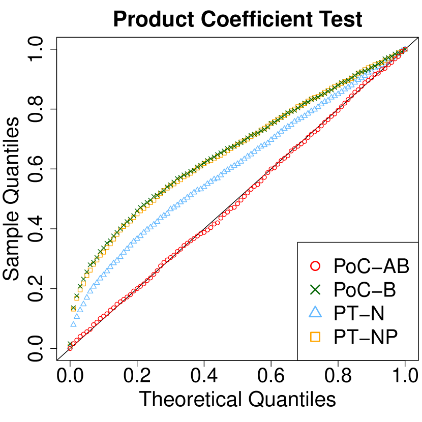
(a) Case 1

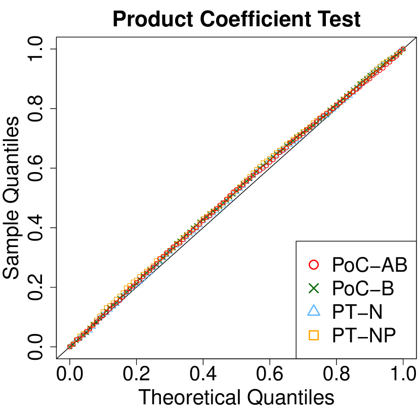
(b) Case 2

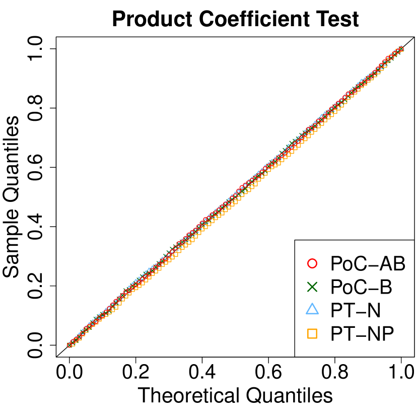
(c) Case 3

(d) Case 4

(e) Case 5

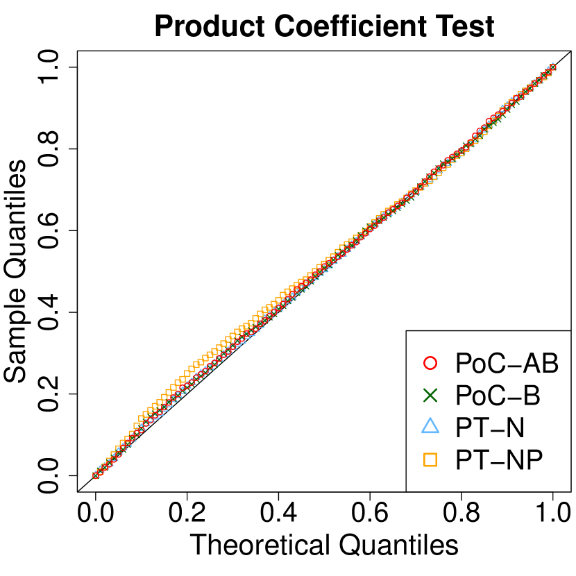
(f) Case 6

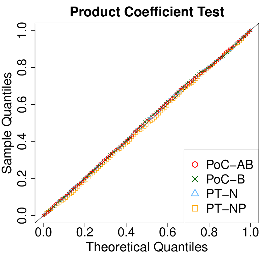
(g) Case 7

Part 2: Statistical power under $H_{A}$.

Under the alternative hypotheses, we consider $\boldsymbol{\alpha}_{S}=a\times\mathbf{1}_{J}$ and $\boldsymbol{\beta}_{M}=b\times\mathbf{1}_{J}$. We fix the size of the mediation effect $\boldsymbol{\alpha}_{S}^{\top}\boldsymbol{\beta}_{M}$ and vary the ratio $a/b$. Figure 10 presents the empirical rejection rates (power) versus the ratio $a/b$ for $n\in\{200,500\}$, respectively. When $n=200$, we fix $\boldsymbol{\alpha}_{S}^{\top}\boldsymbol{\beta}_{M}=0.1$; when $n=500$, we fix $\boldsymbol{\alpha}_{S}^{\top}\boldsymbol{\beta}_{M}=0.04$.

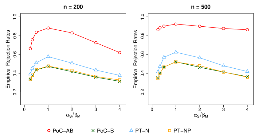
Figure 10: Empirical rejection rates (power) versus $a/b$

Appendix E Extensions Beyond Linear Models

This section provides supplementary details to Sections 5.2 and 5.3 of the main text.

E.1 Supplementary Theoretical Details

Condition 5

The link function $h^{-1}(\cdot)$ in (14) is strictly monotone. Moreover, let $P_{\nu}(M\leqslant m)$ denote the cumulative distribution function of $M\mid\tau_{S}S+\boldsymbol{X}^{\top}\boldsymbol{\alpha}_{\boldsymbol{X}}=\nu$. Assume that given any $m$ in the support of distribution, $P_{\nu}(M\leqslant m)$ is continuously differentiable with respect to $\nu$, and $\frac{\partial P_{\nu}(M\leqslant m)}{\partial\nu}$ is always positive or always negative when $P_{\nu}(M\leqslant m)$ is not a constant with respect to $\nu$.

Condition 5 can be satisfied under various distributions. (i) Bernoulli distribution (logistic regression): $h^{-1}(\nu)=g(\nu)$. (ii) Normal distribution (linear regression) with fixed variance: $h^{-1}(\nu)=\nu$. (iii) Poisson distribution: $h^{-1}(\nu)=\exp(\nu)$. In the following, Proposition 5 Part 1 shows that the null hypothesis (15) is composite similarly to that under the linear SEMs, and the Part 2 further specifies the singularity issue under the composite null hypothesis.

Condition 6

Let $D_{\alpha}=(S,\boldsymbol{X}^{\top})^{\top}$, $g_{\alpha}=g(S\alpha_{S}+\boldsymbol{X}^{\top}\boldsymbol{\alpha}_{\boldsymbol{X}})$, $D_{\beta}=(M,S,\boldsymbol{X}^{\top})^{\top}$, and $g_{\beta}=g(M\beta_{M}+S\tau_{S}+\boldsymbol{X}^{\top}\boldsymbol{\beta}_{\boldsymbol{X}})$. Assume $\mathrm{E}\{g_{\alpha}(1-g_{\alpha})D_{\alpha}D_{\alpha}^{\top}\}$ and $\mathrm{E}\{g_{\beta}(1-g_{\beta})D_{\beta}D_{\beta}^{\top}\}$ are positive definite matrices with bounded eigenvalues.

Condition 6 is a general regularity condition on the design matrix, which is similar to Condition 1 under linear SEM in the main text.

Remark E.23.

Sections 5.2 and 5.3 consider natural indirect effects/mediation effects conditioning on covariates $\boldsymbol{X}$ following VanderWeele and Vansteelandt (2010). On the other hand, Imai et al. (2010a) proposed to examine the average NIE that marginalizes the distribution of the covariates $\boldsymbol{X}$. Examining the conditional NIE is mainly for technical convenience. The conditional NIE $=0$ can give a sufficient condition for the average NIE $=0$. Some results of conditional NIE could be established for average NIE similarly. For instance, under Scenario II, if $h^{-1}(\cdot)$ is strictly monotone, conclusions in Proposition 8 also hold for the average $\mathrm{NIE}_{s\mid s^{*}}(s):=\int\mathrm{NIE}_{s\mid s^{*}}(s,\boldsymbol{x})\mathrm{d}P_{\boldsymbol{X}}(\boldsymbol{x})$, as the sign of $\mathrm{NIE}_{s\mid s^{*}}(s,\boldsymbol{x})$ for all $\boldsymbol{x}$ are the same. Similarly, under Scenario I, results similar to Proposition 5 can also be established for the average $\mathrm{OR}_{s\mid s^{*}}(s):=\int\mathrm{OR}_{s\mid s^{*}}(s,\boldsymbol{x})\mathrm{d}P_{\boldsymbol{X}}(\boldsymbol{x})$ if $\mathrm{OR}_{s\mid s^{*}}(s,\boldsymbol{x})-1$ is non-negative/non-positive for all $\boldsymbol{x}$. As an example, this could hold when $M$ in (14) is binary and follows a logistic regression model, which is a case studied in Section 5.2 in detail.

Condition 7

Let $D_{\alpha}=(S,\boldsymbol{X}^{\top})^{\top}$ and $g_{\alpha}=g(S\alpha_{S}+\boldsymbol{X}^{\top}\boldsymbol{\alpha}_{\boldsymbol{X}})$. Assume $\mathrm{E}\{g_{\alpha}(1-g_{\alpha})D_{\alpha}D_{\alpha}^{\top}\}$ is a positive definite matrix with bounded eigenvalues. Assume conditions on the model of the outcome $Y$ in Condition 1 in the main text .

Condition 7 is similar to Condition 6 and Condition 1.

E.2 Simulations under Non-Linear Models

Non-linear Scenario I.

For $i=1,\ldots,n$, we generate binary mediators $M_{i}$ and outcomes $Y_{i}$ follow Bernoulli distributions with conditional means $\mathrm{E}(M_{i}\mid S_{i},\boldsymbol{X}_{i})=g(\alpha_{S}S_{i}+\alpha_{I}+\alpha_{X}X_{i})$, and $\mathrm{E}(Y_{i}\mid S_{i},M_{i},\boldsymbol{X}_{i})=g(\beta_{M}M_{i}+\beta_{I}+\beta_{X}X_{i}+\tau_{S}S_{i})$, respectively, where $g(x)=\mathrm{logit}^{-1}(x)=e^{x}/(1+e^{x})$. We take $S_{i}$ and $X_{i}\sim\mathrm{Bernoulli}(0.5)$, independently, $\alpha_{I}=\beta_{I}=-1$, and $\alpha_{X}=\beta_{X}=\tau_{S}=1$. Following the definition in Section 5.2, we examine the NIE when $s=0$, $s^{*}=1$, $X=0$, that is, $\log\mathrm{OR}^{\mathrm{NIE}}_{s\mid s^{*}}(s,\boldsymbol{x})=\log\mathrm{OR}^{\mathrm{NIE}}_{0\mid 1}(0,0)=l(P_{0})-l(P_{1}),$ where $P_{0}=d_{\beta,n}\times g\big{(}\alpha_{I}\big{)}+g(\beta_{I})$, and $P_{1}=d_{\beta}\times g(\alpha_{S}+\alpha_{I})+g(\beta_{I})$. We set $\lambda_{\alpha}=1.9\sqrt{n}/\log n$ and $\lambda_{\beta}=1.9\sqrt{n}/\log n$.

Non-linear Scenario II

For $i=1,\ldots,n$, we generate $M_{i}$ as i.i.d. Bernoulli random variables with the conditional mean $\mathrm{E}(M_{i}\mid S_{i},X_{i})=g(\alpha_{S}S_{i}+\alpha_{I}+\alpha_{X}X_{i})$, and $Y_{i}=\beta_{M}M_{i}+\beta_{I}+\beta_{X}X_{i}+\tau_{S}S_{i}+\epsilon_{i}$. Similarly to the scenario I above, we take $S_{i}$ and $X_{i}\sim$ Bernoulli(0.5) and $\epsilon_{i}\sim N(0,0.5^{2})$ i.i.d., In this case, we test the conditional natural indirect effect in (19) when $x=0$, $s=1$, and $s^{*}=0$, i.e., $\text{NIE}_{1|0}(0)=\beta_{M}\{g(\alpha_{S}+\alpha_{I})-g(\alpha_{I})\}.$ $\lambda_{\alpha}=1.9\sqrt{n}/\log n$ and $\lambda_{\beta}=3.3\sqrt{n}/\log n$.

Results.

(1) Under $H_{0}:$ Type-I error control. We estimate $p$-values under three different types of null hypothesis over 1000 repetitions. We present QQ plots of $p$-values obtained under Scenarios I and II in Figures 11 and 12, respectively. Similarly to the linear cases, we observe that both the classical bootstrap (B) and the adaptive bootstrap (AB) give uniformly distributed $p$-values under $H_{0,1}$ and $H_{0,2}$, whereas under $H_{0,3}$, the classical bootstrap would become overly conservative, and the adaptive bootstrap can still give uniformly distributed $p$-values. Specifically, we fix $\alpha_{S}\beta_{M}=0.5^{2}$ in Scenario I and $\alpha_{S}\beta_{M}=0.25^{2}$ in Scenario II. We observe that the adaptive bootstrap can improve the power of the classical bootstrap.

(2) Under $H_{A}:$ Power. Under the alternative hypotheses, we fix the product $\alpha_{S}\beta_{M}$, and vary the ratio $\alpha_{S}/\beta_{M}$. We present the empirical power versus the ratio $\alpha_{S}/\beta_{M}$ in Figure 13.

Figure 11: Scenario 1: Q-Q plots of $p$-values with $n=500$.

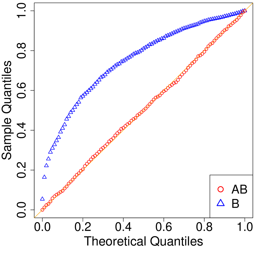
(a) $H_{0,1}:(\alpha_{S},\beta_{M})=(0,0)$

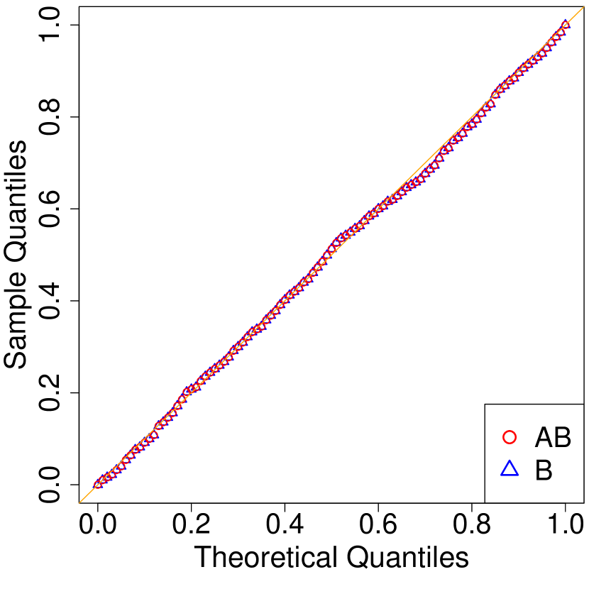
(b) $H_{0,2}:(\alpha_{S},\beta_{M})=(2,0)$

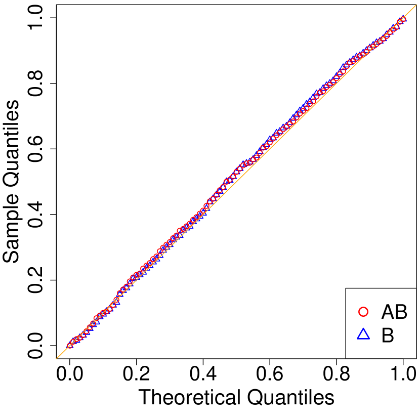
(c) $H_{0,3}:(\alpha_{S},\beta_{M})=(0,2)$

Figure 12: Scenario 2: Q-Q plots of $p$-values with $n=500$.

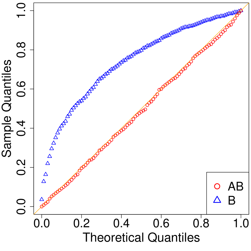
(a) $H_{0,1}:(\alpha_{S},\beta_{M})=(0,0)$

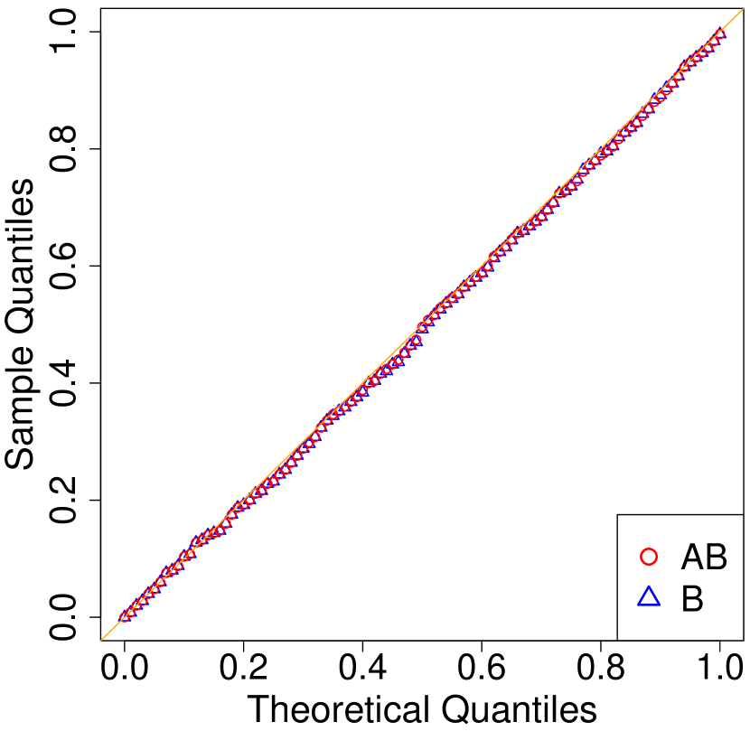
(b) $H_{0,2}:(\alpha_{S},\beta_{M})=(2,0)$

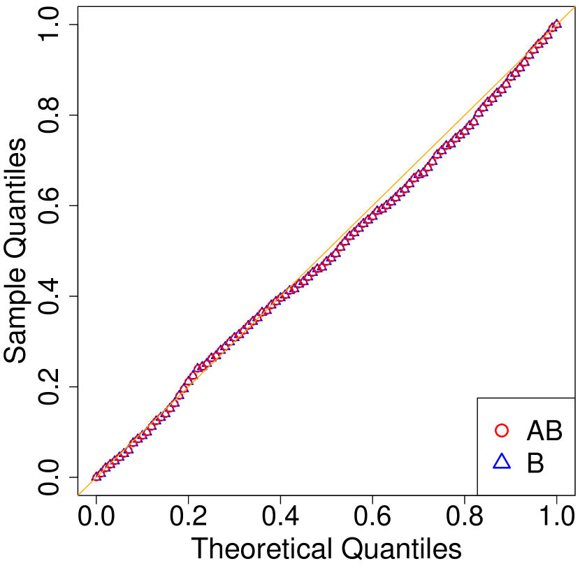
(c) $H_{0,3}:(\alpha_{S},\beta_{M})=(0,2)$

Figure 13: Empirical power versus the ratio $\alpha_{S}/\beta_{M}$.

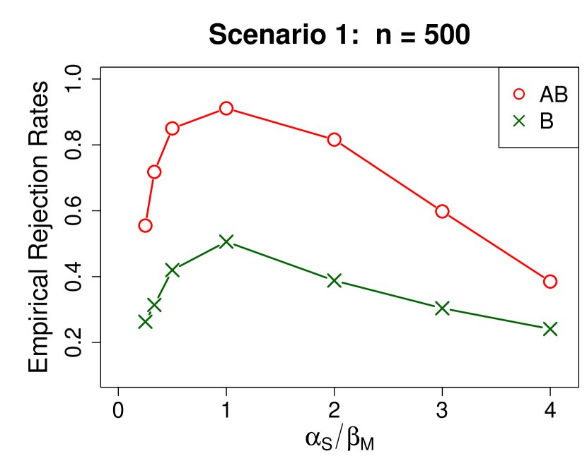
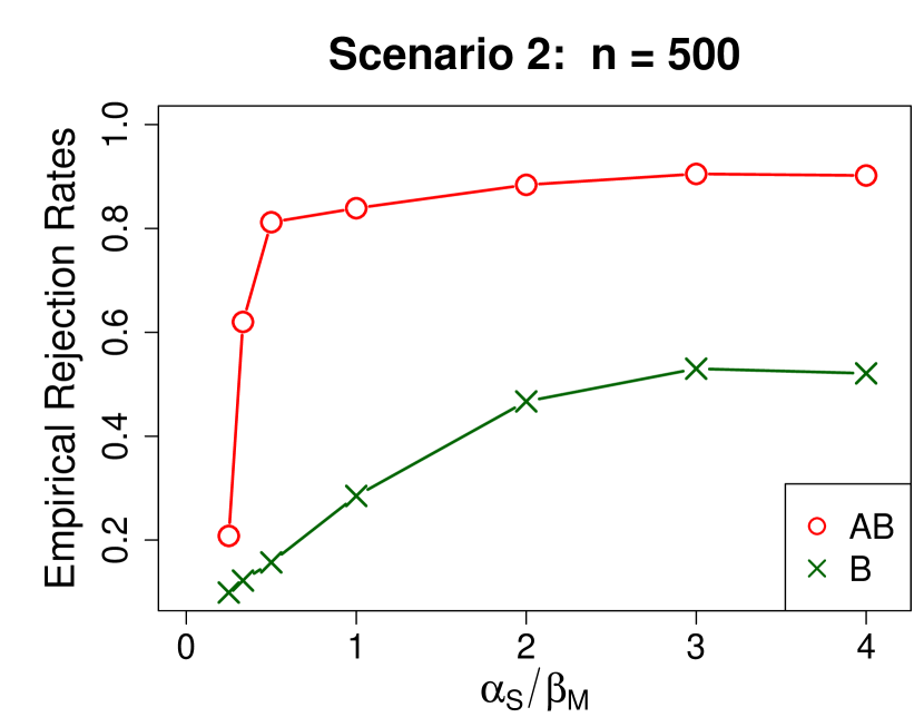
E.3 Proof of Proposition 5

Proof of Part 1.

Let $\phi(m;\nu)$ denote the conditional density of $M\mid(\tau_{S}s+\boldsymbol{X}^{\top}\boldsymbol{\alpha}_{\boldsymbol{X}}=\nu)$. We have

$$P_{s}:= ~{}P\left\{Y(s,M(s))=1\mid\boldsymbol{X}=\boldsymbol{x}\right\}=\int g(\beta_{M}m+\mu_{1,s})\phi(m;\alpha_{S}s+\mu_{2})\mathrm{d}m,$$

$$P_{s^{*}}:= ~{}P\left\{Y(s,M(s^{*}))=1\mid\boldsymbol{X}=\boldsymbol{x}\right\}=\int g(\beta_{M}m+\mu_{1,s})\phi(m;\alpha_{S}s^{*}+\mu_{2})\mathrm{d}m,$$

where we define $\mu_{1,s}=\tau_{S}s+\boldsymbol{x}^{\top}\boldsymbol{\beta}_{\boldsymbol{X}}$, $\mu_{2}=\boldsymbol{x}^{\top}\boldsymbol{\alpha}_{\boldsymbol{X}}$, and $g(x)=\mathrm{logit}^{-1}(x)=e^{x}/(1+e^{x})$. $H_{0}$ in (15) is equivalent to $P_{s}-P_{s^{*}}=0$. First, if $\beta_{M}=0$,

$$P_{s}-P_{s^{*}}=g(\mu_{1,s})\int\big{\{}\phi(m;\alpha_{S}s+\mu_{2})-\phi(m;\alpha_{S}s^{*}+\mu_{2})\big{\}}\mathrm{d}m=0.$$

Second, if $\beta_{M}\neq 0$, $g(\beta_{M}m+\mu_{1,s})>0$. By $g(x)>0$ and the integrated tail probability expectation formula, we have $\mathrm{E}_{X}\{g(X)\}=\int g(X)\mathrm{d}F(X)=\int_{0}^{\infty}P\{g(X)>t\}\mathrm{d}t$ for any integrable random variable $X$. It follows that

$$P_{s}-P_{s^{*}}=\int_{0}^{\infty}\Big{[}P_{\alpha_{S}s+\mu_{2}}\big{\{}g(\beta_{M}M+\mu_{1,s})>t\big{\}}-P_{\alpha_{S}s^{*}+\mu_{2}}\big{\{}g(\beta_{M}M+\mu_{1,s})>t\big{\}}\Big{]}\mathrm{d}t$$

where for $\nu=\alpha_{S}s+\mu_{2}$ or $\nu=\alpha_{S}s^{*}+\mu_{2}$, we define

$$P_{\nu}\Big{\{}g(\beta_{M}M+\mu_{1,s})>t\Big{\}}= ~{}\int\mathrm{I}\big{\{}g(\beta_{M}M+\mu_{1,s})>t\big{\}}\phi(m;\nu)\mathrm{d}m$$

$$= ~{}P_{\nu}\Big{\{}\beta_{M}M>g^{-1}(t)-\mu_{1,s}\Big{\}},$$

where the second equation holds as $g(x)$ is strictly increasing. By Condition 5, given any $m$, $P_{\nu}(\beta_{M}M>m)$ is strictly monotone in $\nu$. Therefore, when $\beta_{M}\neq 0$, $P_{s}-P_{s^{*}}=0$ if and only if $\alpha_{S}s+\mu_{1,s}=\alpha_{S}s^{*}+\mu_{1,s}\Leftrightarrow\alpha_{S}=0$. In summary, $H_{0}$ (15) holds for $s\neq s^{*}$ if and only if $\alpha_{S}=0$ or $\beta_{M}=0$.

Proof of Part 2.

For the simplicity of notation, we let $P_{s}=P\left\{Y(s,M(s))=1\mid\boldsymbol{X}\right\}$ and $P_{s^{*}}=P\left\{Y(s,M(s))=1\mid\boldsymbol{X}\right\}$. For the parameter $\theta\in\{\alpha_{S},\beta_{M}\}$,

$$\frac{\partial\log\mathrm{NIE}}{\partial\theta}=\frac{1}{P_{s}(1-P_{s})}\frac{\partial P_{s}}{\partial\theta}-\frac{1}{P_{s^{*}}(1-P_{s^{*}})}\frac{\partial P_{s^{*}}}{\partial\theta}.$$ (55)

(i.1) When $\alpha_{S}=0$, $P_{s}=P_{s^{*}}$ and $\phi(m;\alpha_{S}s+\mu_{2})=\phi(m;\alpha_{S}s^{*}+\mu_{2})$, where $\mu_{2}=\boldsymbol{X}^{\top}\boldsymbol{\alpha}_{\boldsymbol{X}}$. By $\alpha_{S}=0$,

$$\frac{\partial P_{s}}{\partial\beta_{M}}= \int\frac{g(\beta_{M}m+\mu_{1,s})}{\partial\beta_{M}}\phi(m;\alpha_{S}s+\mu_{2})\mathrm{d}m=\int g^{\prime}(\beta_{M}m+\mu_{1,s})m\phi(m;\mu_{2})\mathrm{d}m,$$

$$\frac{\partial P_{s^{*}}}{\partial\beta_{M}}= \int\frac{g(\beta_{M}m+\mu_{1,s})}{\partial\beta_{M}}\phi(m;\alpha_{S}s^{*}+\mu_{2})\mathrm{d}m=\int g^{\prime}(\beta_{M}m+\mu_{1,s})m\phi(m;\mu_{2})\mathrm{d}m,$$

where $g^{\prime}(x)=e^{x}/(1+e^{x})^{2}$. It follows that $\frac{\partial P_{s}}{\partial\beta_{M}}=\frac{\partial P_{s^{*}}}{\partial\beta_{M}}\mid_{\alpha_{S}=0}$. By (55), $\frac{\partial\log\mathrm{NIE}}{\partial\beta_{M}}\mid_{\alpha_{S}=0}=0$.

(i.2) When $\beta_{M}=0$, we have $P_{s}=\int g(\mu_{1,s})\phi(m;\alpha_{S}s+\mu_{2})\mathrm{d}m=g(\mu_{1,s}),$ where we use $\int\phi(m;\alpha_{S}s+\mu_{2})\mathrm{d}m=1$ by the property of density. Similarly, we have $P_{s^{*}}=P_{s}=g(\mu_{1,s})$. Moreover, when $\beta_{M}=0$,

$$\frac{\partial P_{s}}{\partial\alpha_{S}}\biggr{|}_{\beta_{M}=0}= ~{}\int g(\beta_{M}m+\mu_{1,s})\frac{\partial\phi(m;\alpha_{S}s+\mu_{2})}{\partial\alpha_{S}}\mathrm{d}m\biggr{|}_{\beta_{M}=0}=g(\mu_{1,s})\int\frac{\partial\phi(m;\alpha_{S}s+\mu_{2})}{\partial\alpha_{S}}\mathrm{d}m,$$

so $\frac{\partial P_{s}}{\partial\alpha_{S}}=\frac{\partial P_{s^{*}}}{\partial\alpha_{S}}\mid_{\beta_{M}=0}.$ By (55), $\frac{\partial\log\mathrm{NIE}}{\partial\alpha_{S}}\mid_{\beta_{M}=0}=0$.

• When $\alpha_{S}=0$ and $\beta_{M}\neq 0$, we have $P_{s}=P_{s^{*}}$, and by (55),

  $$\frac{\partial\log\mathrm{NIE}}{\partial\alpha_{S}}=\frac{1}{P_{s}(1-P_{s})}\left(\frac{\partial P_{s}}{\partial\alpha_{S}}-\frac{\partial P_{s^{*}}}{\partial\alpha_{S}}\right).$$

  When $\alpha_{S}=0$, we have

  $$\left(\frac{\partial P_{s}}{\partial\alpha_{S}}-\frac{\partial P_{s^{*}}}{\partial\alpha_{S}}\right)\biggr{|}_{\alpha_{S}=0}=(s-s^{*})\int_{0}^{\infty}\frac{\partial P_{\nu}\big{\{}\beta_{M}M>g^{-1}(t)-\mu_{1,s}\big{\}}}{\partial\nu}\biggr{|}_{\nu=\mu_{2}}\mathrm{d}t\neq 0$$

  which follows by Condition 5.

• When $\beta_{M}=0$ and $\alpha_{S}\neq 0$, we have $P_{s}=P_{s^{*}}$,

  $$\left(\frac{\partial P_{s}}{\partial\beta_{M}}-\frac{\partial P_{s^{*}}}{\partial\beta_{M}}\right)\biggr{|}_{\beta_{M}=0}= g^{\prime}(\mu_{1,s})\int m\big{\{}\phi(m;\alpha_{S}s+\mu_{2})-\phi(m;\alpha_{S}s^{*}+\mu_{2})\big{\}}\mathrm{d}m,$$

  $$= g^{\prime}(\mu_{1,s})\big{\{}h^{-1}(\alpha_{S}s+\mu_{2})-h^{-1}(\alpha_{S}s^{*}+\mu_{2})\big{\}}$$ (56)

  which is obtained by the definition of calculating population mean and the model (14). When $h^{-1}(\cdot)$ is strictly monotone, by $g^{\prime}(\mu_{1,s})>0$, $\eqref{eq:partialbetadiff}\neq 0$.

E.4 Proof of Proposition 8

Proof of Part 1.

The conclusion follows by the form of $\mathrm{NIE}$ in (19).

Proof of Part 2.

Note that

$$\frac{\partial\mathrm{NIE}}{\partial\alpha_{S}}= ~{}\beta_{M}\Big{\{}g^{\prime}\big{(}\alpha_{S}s+\boldsymbol{x}^{\top}\boldsymbol{\alpha}_{\boldsymbol{X}}\big{)}\times s-g^{\prime}\big{(}\alpha_{S}s^{*}+\boldsymbol{x}^{\top}\boldsymbol{\alpha}_{\boldsymbol{X}}\big{)}\times s^{*}\Big{\}}$$

$$\frac{\partial\mathrm{NIE}}{\partial\beta_{M}}= ~{}g\big{(}\alpha_{S}s+\boldsymbol{x}^{\top}\boldsymbol{\alpha}_{\boldsymbol{X}}\big{)}-g\big{(}\alpha_{S}s^{*}+\boldsymbol{x}^{\top}\boldsymbol{\alpha}_{\boldsymbol{X}}\big{)}$$

where $g^{\prime}(x)=e^{x}(1+e^{x})^{2}$.
(i) $\frac{\partial\mathrm{NIE}}{\partial\alpha_{S}}\mid_{\beta_{M}=0}=0$ and $\frac{\partial\mathrm{NIE}}{\partial\alpha_{S}}\mid_{\alpha_{S}=0}=g(\boldsymbol{x}^{\top}\boldsymbol{\alpha}_{\boldsymbol{X}})-g(\boldsymbol{x}^{\top}\boldsymbol{\alpha}_{\boldsymbol{X}})=0$.
(ii) $\frac{\partial\mathrm{NIE}}{\partial\alpha_{S}}\mid_{\alpha_{S}=0,\beta_{M}\neq 0}=\beta_{M}g^{\prime}(\boldsymbol{x}^{\top}\boldsymbol{\alpha}_{\boldsymbol{X}})(s-s^{*})\neq 0$ when $s\neq s^{*}$.
(iii) $\frac{\partial\mathrm{NIE}}{\partial\beta_{M}}\mid_{\alpha_{S}\neq 0,\beta_{M}=0}=g(\alpha_{S}s+\boldsymbol{x}^{\top}\boldsymbol{\alpha}_{\boldsymbol{X}})-g(\alpha_{S}s^{*}+\boldsymbol{x}^{\top}\boldsymbol{\alpha}_{\boldsymbol{X}})\neq 0$, which follows by the strict monotonicity of the function $g(x)$.

E.5 Proof of Theorem 6

By the definition $P_{s}=P\left\{Y(s,M(s))=1\mid\boldsymbol{X}=\boldsymbol{x}\right\}$ and the model (16),

$$P_{s}= ~{}\sum_{m\in\{0,1\}}P(Y(s,m)=1\mid M(s)=m,\boldsymbol{X}=\boldsymbol{x})P(M(s)=m\mid\boldsymbol{X}=\boldsymbol{x})$$

$$= ~{}\sum_{m\in\{0,1\}}g(\beta_{M,n}m+\boldsymbol{x}^{\top}\boldsymbol{\beta}_{\boldsymbol{X}}+\tau_{S}s)\big{\{}g\big{(}\alpha_{S,n}s+\boldsymbol{x}^{\top}\boldsymbol{\alpha}_{\boldsymbol{X}}\big{)}\big{\}}^{m}\big{\{}1-g\big{(}\alpha_{S,n}s+\boldsymbol{x}^{\top}\boldsymbol{\alpha}_{\boldsymbol{X}}\big{)}\big{\}}^{1-m}$$

$$= ~{}g(\beta_{M,n}+\boldsymbol{x}^{\top}\boldsymbol{\beta}_{\boldsymbol{X}}+\tau_{S}s)g\big{(}\alpha_{S,n}s+\boldsymbol{x}^{\top}\boldsymbol{\alpha}_{\boldsymbol{X}}\big{)}+g(\boldsymbol{x}^{\top}\boldsymbol{\beta}_{\boldsymbol{X}}+\tau_{S}s)\big{\{}1-g\big{(}\alpha_{S,n}s+\boldsymbol{x}^{\top}\boldsymbol{\alpha}_{\boldsymbol{X}}\big{)}\big{\}}$$

$$= ~{}d_{\beta,n}\times g\big{(}\alpha_{S,n}s+\boldsymbol{x}^{\top}\boldsymbol{\alpha}_{\boldsymbol{X}}\big{)}+g(\boldsymbol{x}^{\top}\boldsymbol{\beta}_{\boldsymbol{X}}+\tau_{S}s),$$

where for the simplicity of notation, we define $d_{\beta,n}=g(\beta_{M,n}+\boldsymbol{x}^{\top}\boldsymbol{\beta}_{\boldsymbol{X}}+\tau_{S}s)-g(\boldsymbol{x}^{\top}\boldsymbol{\beta}_{\boldsymbol{X}}+\tau_{S}s)$. Similarly, by $P_{s^{*}}=P\left\{Y(s,M(s))=1\mid\boldsymbol{X}=\boldsymbol{x}\right\}$,

$$P_{s^{*}}= ~{}\sum_{m\in\{0,1\}}P(Y(s,m)=1\mid M(s^{*})=m,\boldsymbol{X}=\boldsymbol{x})P(M(s^{*})=m\mid\boldsymbol{X}=\boldsymbol{x})$$

$$= ~{}\sum_{m\in\{0,1\}}g(\beta_{M,n}m+\boldsymbol{x}^{\top}\boldsymbol{\beta}_{\boldsymbol{X}}+\tau_{S}s)\big{\{}g\big{(}\alpha_{S,n}s^{*}+\boldsymbol{x}^{\top}\boldsymbol{\alpha}_{\boldsymbol{X}}\big{)}\big{\}}^{m}\big{\{}1-g\big{(}\alpha_{S,n}s^{*}+\boldsymbol{x}^{\top}\boldsymbol{\alpha}_{\boldsymbol{X}}\big{)}\big{\}}^{1-m}$$

$$= ~{}d_{\beta,n}\times g\big{(}\alpha_{S,n}s^{*}+\boldsymbol{x}^{\top}\boldsymbol{\alpha}_{\boldsymbol{X}}\big{)}+g(\boldsymbol{x}^{\top}\boldsymbol{\beta}_{\boldsymbol{X}}+\tau_{S}s).$$

By consistency of regression coefficients of the logistic regressions, we have $\hat{P}_{r}-P_{r}=O_{p}(n^{-1/2})$ for $r\in\{s,s^{*}\}$.

Let $l(x)=\log\frac{x}{1-x}$ and its derivative is $l^{\prime}(x)=\frac{1}{x(1-x)}$. By $\hat{P}_{r}-P_{r}=o_{p}(1)$ for $r\in\{s,s^{*}\}$ and Taylor’s expansion,

$$\widehat{\mathrm{NIE}}-\mathrm{NIE}= ~{}l(\hat{P}_{s})-l(\hat{P}_{s^{*}})-l(P_{s})+l(P_{s^{*}})$$

$$= ~{}\big{\{}l^{\prime}(P_{s})(\hat{P}_{s}-P_{s})-l^{\prime}(P_{s^{*}})(\hat{P}_{s^{*}}-P_{s^{*}})\big{\}}\times\{1+O_{p}(n^{-1/2})\}.$$ (57)

In particular, for $r\in\{s,s^{*}\}$, we have

$$\hat{P}_{r}-P_{r}= ~{}\hat{d}_{{\beta}}\times g\big{(}\hat{\alpha}_{S}r+\boldsymbol{x}^{\top}\hat{\boldsymbol{\alpha}}_{\boldsymbol{X}}\big{)}-d_{\beta,n}\times g\big{(}\alpha_{S,n}r+\boldsymbol{x}^{\top}\boldsymbol{\alpha}_{\boldsymbol{X}}\big{)}$$

$$~{}+g(\boldsymbol{x}^{\top}\hat{\boldsymbol{\beta}}_{\boldsymbol{X}}+\hat{\tau}_{S}s)-g(\boldsymbol{x}^{\top}\boldsymbol{\beta}_{\boldsymbol{X}}+\tau_{S}s),$$

where we define $\hat{d}_{{\beta}}=g(\hat{\beta}_{M}+\boldsymbol{x}^{\top}\hat{\boldsymbol{\beta}}_{\boldsymbol{X}}+\hat{\tau}_{S}s)-g(\boldsymbol{x}^{\top}\hat{\boldsymbol{\beta}}_{\boldsymbol{X}}+\hat{\tau}_{S}s)$, and $(\hat{\beta}_{M},\hat{\beta}_{\boldsymbol{X}},\hat{\tau}_{S})$ denote sample estimates of $({\beta}_{M},{\beta}_{\boldsymbol{X}},{\tau}_{S})$ under the logistic regression. As $P_{s}=P_{s^{*}}$ under $H_{0}$,

$$\eqref{eq:loghatdiff}= ~{}l^{\prime}(P_{s})\{(\hat{P}_{s}-P_{s})-(\hat{P}_{s^{*}}-P_{s^{*}})\}\times\{1+O_{p}(n^{-1/2})\}$$

$$= ~{}l^{\prime}(P_{s})\big{(}\hat{d}_{{\alpha}}\hat{d}_{{\beta}}-d_{\alpha,n}d_{\beta,n}\big{)}\times\big{\{}1+O_{p}(n^{-1/2})\big{\}},$$

where we define $d_{\alpha,n}=g(\alpha_{S,n}s+\boldsymbol{x}^{\top}\boldsymbol{\alpha}_{\boldsymbol{X}})-g(\alpha_{S,n}s^{*}+\boldsymbol{x}^{\top}\boldsymbol{\alpha}_{\boldsymbol{X}})$, $\hat{d}_{\alpha}=g(\hat{\alpha}_{S}s+\boldsymbol{x}^{\top}\hat{\boldsymbol{\alpha}}_{\boldsymbol{X}})-g(\hat{\alpha}_{S}s^{*}+\boldsymbol{x}^{\top}\hat{\boldsymbol{\alpha}}_{\boldsymbol{X}})$, and $(\hat{\alpha}_{S},\hat{\boldsymbol{\alpha}}_{\boldsymbol{X}})$ denote sample estimates of $({\alpha}_{S},{\boldsymbol{\alpha}}_{\boldsymbol{X}})$ under the logistic regression. To analyze the asymptotic property of $\eqref{eq:loghatdiff}$, we next discuss under three cases of $H_{0}$, respectively.

(i) When $\alpha_{S}\neq 0$ and $\beta_{M}=0$, we have $d_{\beta,n}\to d_{\beta}=0$, whereas $d_{\alpha,n}\to d_{\alpha}\neq 0$ by strict monotonicity of the function $g(\cdot)$. Moreover, by $d_{\beta}=0$, $l^{\prime}(P_{s})$ and $l^{\prime}(P_{s^{*}})\to\gamma_{0}=l^{\prime}\{g(\boldsymbol{x}^{\top}\boldsymbol{\beta}_{\boldsymbol{X}}+\tau_{S}s)\}\}\neq 0$ as $n\to\infty$. Therefore, as $n\to\infty$,

$$\sqrt{n}\times\eqref{eq:loghatdiff}\to ~{}\gamma_{0}\times d_{\alpha}\times\sqrt{n}(\hat{d}_{{\beta}}-0)\xrightarrow{d}\gamma_{0}\times d_{\alpha}\times Z_{\beta}.$$

(ii) When $\alpha_{S}=0$, and $\beta_{M}\neq 0$, we have $d_{\alpha,n}\to d_{\alpha}=0$, whereas $d_{\beta,n}\to d_{\beta}\neq 0$ by strict monotonicity of the function $g(\cdot)$. Moreover, $l^{\prime}(P_{s})$ and $l^{\prime}(P_{s^{*}})\to\gamma_{0}=l^{\prime}\{d_{\beta_{M}}g(\boldsymbol{x}^{\top}\boldsymbol{\alpha}_{\boldsymbol{X}}\big{)}+g(\boldsymbol{x}^{\top}\boldsymbol{\beta}_{\boldsymbol{X}}+\tau_{S}s)\}\neq 0$, and

$$\sqrt{n}\times\eqref{eq:loghatdiff}\to ~{}\gamma_{0}\times\sqrt{n}(\hat{d}_{{\alpha}}-0)\times d_{\beta}\xrightarrow{d}\gamma_{0}\times Z_{\alpha}\times d_{\beta}.$$

(iii) When $\alpha_{S}=\beta_{M}=0$, $l^{\prime}(P_{s})$ and $l^{\prime}(P_{s^{*}})\to\gamma_{0}=l^{\prime}\{g(\boldsymbol{x}^{\top}\boldsymbol{\beta}_{\boldsymbol{X}}+\tau_{S}s)\}\neq 0$, and

$$\sqrt{n}d_{\alpha,n}= \sqrt{n}\left\{g(\alpha_{S,n}s+\boldsymbol{x}^{\top}\boldsymbol{\alpha}_{\boldsymbol{X}})-g(\alpha_{S,n}s^{*}+\boldsymbol{x}^{\top}\boldsymbol{\alpha}_{\boldsymbol{X}})\right\}\to g^{\prime}(\boldsymbol{x}^{\top}\boldsymbol{\alpha}_{\boldsymbol{X}})(s-s^{*})b_{\alpha}=d_{b_{\alpha}},$$

$$\sqrt{n}d_{\beta,n}= \sqrt{n}\left\{g(\beta_{M,n}s+\boldsymbol{x}^{\top}\boldsymbol{\beta}_{\boldsymbol{X}}+\tau_{S}s)-g(\beta_{M,n}s^{*}+\boldsymbol{x}^{\top}\boldsymbol{\beta}_{\boldsymbol{X}}+\tau_{S}s)\right\}$$

$$\to g^{\prime}(\boldsymbol{x}^{\top}\boldsymbol{\beta}_{\boldsymbol{X}}+\tau_{S}s)(s-s^{*})b_{\beta}=d_{b_{\beta}}.$$

It follows that

$$n\times\eqref{eq:loghatdiff}\to ~{}\gamma_{0}\Big{\{}d_{b_{\alpha}}\sqrt{n}(\hat{d}_{{\beta}}-0)+d_{b_{\beta}}\sqrt{n}(\hat{d}_{{\alpha}}-0)+\sqrt{n}(\hat{d}_{{\alpha}}-0)\times\sqrt{n}(\hat{d}_{{\beta}}-0)\Big{\}}$$

$$\xrightarrow{d} ~{}\gamma_{0}\left(d_{b_{\alpha}}Z_{\beta}+d_{b_{\beta}}Z_{\alpha}+Z_{\alpha}Z_{\beta}\right).$$

Lemma E.24 (Individual limits of $\hat{d}_{\alpha}$ and $\hat{d}_{\beta}$.).

Under the condition of Theorem 6,

$$\sqrt{n}(\hat{d}_{{\alpha}}-d_{\alpha,n})\xrightarrow{d}Z_{\alpha},\hskip 20.00003pt\sqrt{n}(\hat{d}_{{\beta}}-d_{\beta,n})\xrightarrow{d}Z_{\beta},$$

where $Z_{\alpha}=W_{\alpha}^{\top}B_{\alpha}$, $Z_{\beta}=W_{\beta}^{\top}B_{\beta}$, $B_{\alpha}$ and $B_{\beta}$ represent mean-zero multivariate normal distributions specified in (58) and (60), respectively, and $W_{\alpha}$ and $W_{\beta}$ are vectors defined in (59) and (61), respectively.

Proof of Lemma E.24. By Taylor’s expansion and the property of logistic regression, we have

$$\sqrt{n}\begin{pmatrix}\hat{\alpha}_{S}-\alpha_{S,n}\\ \hat{\boldsymbol{\alpha}}_{\boldsymbol{X}}-\boldsymbol{\alpha}_{\boldsymbol{X}}\end{pmatrix}= \sqrt{n}\left\{\sum_{i=1}^{n}g_{\alpha,i}(1-g_{\alpha,i})D_{\alpha,i}D_{\alpha,i}^{\top}\right\}^{-1}\left\{\sum_{i=1}^{n}(M_{i}-g_{\alpha,i})D_{\alpha,i}\right\}\{1+o_{p}(1)\}$$

$$\xrightarrow{d} B_{\alpha},$$ (58)

where in the first equation, we define $D_{\alpha,i}=(S_{i},\boldsymbol{X}_{i}^{\top})^{\top}$ and $g_{\alpha,i}=g(S_{i}\alpha_{S}+\boldsymbol{X}_{i}^{\top}\boldsymbol{\alpha}_{\boldsymbol{X}})$, and in (58), $B_{\alpha}$ represents a multivariate normal distribution with $\mathrm{E}(B_{\alpha})=\mathbf{0}$ and $\mathrm{cov}(B_{\alpha})=\mathrm{cov}\{V_{\alpha}^{-1}(M-g_{\alpha})D_{\alpha}\}$, where we define $D_{\alpha}=(S,\boldsymbol{X}^{\top})^{\top}$, $g_{\alpha}=g(S\alpha_{S}+\boldsymbol{X}^{\top}\boldsymbol{\alpha}_{\boldsymbol{X}})$, and $V_{\alpha}=\mathrm{E}\big{\{}g_{\alpha}(1-g_{\alpha})D_{\alpha}D_{\alpha}^{\top}\big{\}}$. By Taylor’s expansion,

$$\sqrt{n}(\hat{d}_{{\alpha}}-d_{\alpha})= ~{}{W}_{\alpha}^{\top}\times\sqrt{n}\begin{pmatrix}\hat{\alpha}_{S}-\alpha_{S,n}\\ \hat{\boldsymbol{\alpha}}_{\boldsymbol{X}}-{\boldsymbol{\alpha}}_{\boldsymbol{X},n}\end{pmatrix}\{1+o_{p}(1)\},$$

where we define $\mu_{s,\alpha}=\alpha_{S}s+\boldsymbol{x}^{\top}\boldsymbol{\alpha}_{\boldsymbol{X}}$, $\mu_{s^{*},\alpha}=\alpha_{S}s^{*}+\boldsymbol{x}^{\top}\boldsymbol{\alpha}_{\boldsymbol{X}}$, and

$${W}_{\alpha}^{\top}=g^{\prime}(\mu_{s,\alpha})\times\big{(}s,\,\boldsymbol{x}^{\top}\big{)}-g^{\prime}(\mu_{s^{*},\alpha})\times\big{(}s^{*},\,\boldsymbol{x}^{\top}\big{)}.$$ (59)

Therefore, by (58), $\sqrt{n}(\hat{d}_{{\alpha}}-d_{\alpha})\xrightarrow{d}W_{\alpha}^{\top}B_{\alpha}=Z_{\alpha}$.

Similarly, by Taylor’s expansion,

$$\sqrt{n}\begin{pmatrix}\hat{\beta}_{M}-\beta_{M,n}\\ \hat{\boldsymbol{\beta}}_{\boldsymbol{X}}-{\boldsymbol{\beta}}_{\boldsymbol{X}}\\ \hat{\tau}_{S}-\tau_{S}\end{pmatrix}= \left\{\sum_{i=1}^{n}g_{\beta,i}(1-g_{\beta,i})D_{\beta,i}D_{\beta,i}^{\top}\right\}^{-1}\left\{\sum_{i=1}^{n}(Y_{i}-g_{\beta,i})D_{\beta,i}\right\}\{1+o_{p}(1)\}$$

$$\xrightarrow{d} B_{\beta},$$ (60)

where in the first equation, we define $D_{\beta,i}=(M_{i},S_{i},\boldsymbol{X}_{i}^{\top})^{\top}$, $g_{\beta,i}=g(M_{i}\beta_{M}+S_{i}\tau_{S}+\boldsymbol{X}_{i}^{\top}\boldsymbol{\beta}_{\boldsymbol{X}})$, and in (60), $B_{\beta}$ represents a normal distribution with $\mathrm{E}(B_{\beta})=\mathbf{0}$ and $\mathrm{cov}(B_{\beta})=\mathrm{cov}\{V_{\beta}^{-1}(Y-g_{\beta})D_{\beta}\}$, where we define $g_{\beta}=g(M\beta_{M}+S\tau_{S}+\boldsymbol{X}^{\top}\boldsymbol{\beta}_{\boldsymbol{X}})$, $D_{\beta}=(M,S,\boldsymbol{X}^{\top})^{\top}$, and $V_{\beta}=\mathrm{E}\big{\{}g_{\beta}(1-g_{\beta})D_{\beta}D_{\beta}^{\top}\big{\}}$. Moreover, by Taylor’s expansion,

$$\sqrt{n}(\hat{d}_{\beta}-d_{\beta,n})=W_{\beta}^{\top}\times\sqrt{n}\begin{pmatrix}\hat{\beta}_{M}-\beta_{M,n}\\ \hat{\boldsymbol{\beta}}_{\boldsymbol{X}}-{\boldsymbol{\beta}}_{\boldsymbol{X}}\\ \hat{\tau}_{S}-\tau_{S}\end{pmatrix}\times\{1+o_{p}(1)\},$$

where we define $\mu_{0,\beta}=\boldsymbol{x}^{\top}\boldsymbol{\alpha}_{\boldsymbol{X}}+s\tau_{S}$, $\mu_{1,\beta}=\beta_{M}+\mu_{0,\beta}$, and

$${W}_{\beta}^{\top}=g^{\prime}(\mu_{1,\beta})\times\big{(}1,\,\boldsymbol{x}^{\top},\,s\big{)}-g^{\prime}(\mu_{0,\beta})\times\big{(}0,\,\boldsymbol{x}^{\top},\,s\big{)}.$$ (61)

Therefore, by (58), $\sqrt{n}(\hat{d}_{{\beta}}-d_{\beta,n})\xrightarrow{d}W_{\beta}^{\top}B_{\beta}=Z_{\beta}$.

E.6 Proof of Theorem 7

Notation. Define $(\mathbb{Z}_{\alpha}^{*},\mathbb{Z}_{\beta}^{*})$ as the bootstrap counterparts of $(Z_{\alpha},Z_{\beta})$. In particular, by the definitions of $Z_{\alpha}$ and $Z_{\beta}$ in Lemma E.24, we let $\mathbb{Z}_{\alpha}^{*}={W}_{\alpha}^{*\top}\left[\mathbb{P}_{n}^{*}\{g_{\alpha}(1-g_{\alpha})D_{\alpha}D_{\alpha}^{\top}\}\right]^{-1}\times\mathbb{G}_{n}^{*}\{(M-g_{\alpha})D_{\alpha}\}$ and $\mathbb{Z}_{\beta}^{*}={W}_{\beta}^{*\top}[\mathbb{P}_{n}^{*}\{g_{\beta}(1-g_{\beta})D_{\beta}D_{\beta}^{\top}]^{-1}\times\mathbb{G}_{n}^{*}\{(M-g_{\beta})D_{\beta}\},$ where $D_{\alpha}$, $D_{\beta}$, $g_{\alpha}$, and $g_{\beta}$ are defined in Condition 6, and ${W}_{\alpha}^{*\top}$ and ${W}_{\beta}^{*\top}$ represent bootstrap estimators of ${W}_{\alpha}^{\top}$ in (59) and ${W}_{\beta}^{\top}$ in (61), respectively. Specifically, ${W}_{\alpha}^{*\top}=g^{\prime}(\hat{\mu}_{s,\alpha}^{*})\times(s,\,\boldsymbol{x}^{\top})-g^{\prime}(\hat{\mu}_{s^{*},\alpha}^{*})\times(s^{*},\,\boldsymbol{x}^{\top})$ and ${W}_{\beta}^{*\top}=g^{\prime}(\hat{\mu}_{1,\beta}^{*})\times(1,\,\boldsymbol{x}^{\top},\,s)-g^{\prime}(\hat{\mu}_{0,\beta}^{*})\times(0,\,\boldsymbol{x}^{\top},\,s)$, where $(\hat{\mu}_{s^{*},\alpha}^{*},\hat{\mu}_{s^{*},\alpha}^{*},\hat{\mu}_{1,\beta}^{*},\hat{\mu}_{0,\beta}^{*})$ represent bootstrap estimators of $({\mu}_{s^{*},\alpha},{\mu}_{s^{*},\alpha},{\mu}_{1,\beta},{\mu}_{0,\beta})$. The definitions are similar to $\mathbb{Z}_{S,n}^{*}$ and $\mathbb{Z}_{M,n}^{*}$ in Section 3. Moreover, $\hat{\gamma}_{0}^{*}=\{\hat{P}_{*}^{*}(1-\hat{P}_{*}^{*})\}^{-1}$, where $\hat{P}_{*}^{*}=g(\boldsymbol{x}^{\top}\hat{\boldsymbol{\beta}}_{\boldsymbol{X}}^{*}+\hat{\tau}_{S}^{*}s)$, and $\hat{\boldsymbol{\beta}}_{\boldsymbol{X}}^{*}$ and $\hat{\tau}_{S}^{*}$ denote non-parametric bootstrap estimators of $\boldsymbol{\beta}_{\boldsymbol{X}}$ and ${\tau}_{S}$, respectively.

Proof. The proof is very similar to that of Theorem 2. We describe the key steps, and the details follow similarly to that in Section C.3. When $(\alpha_{S},\beta_{M})\neq(0,0)$, the bootstrap estimator $\widehat{\text{NIE}}^{*}$ is consistent by the asymptotic expansion in Section E.5 and asymptotic normality. When $(\alpha_{S},\beta_{M})=(0,0)$, the bootstrap estimator $(d_{b_{\alpha}}\mathbb{Z}_{\beta}^{*}+d_{b_{\beta}}\mathbb{Z}_{\alpha}^{*}+\mathbb{Z}_{\alpha}^{*}\mathbb{Z}_{\beta}^{*})\hat{\gamma}_{0}^{*}$ is consistent by the asymptotic expansion in E.5 and its limit form. To prove Theorem 7, results similar to (37) can be established as under the logistic models by the asymptotic normality in (58) and (60). Then the proof follows by the arguments in Section C.3.

E.7 Proof of Theorem 9

Note that $\widehat{\mathrm{NIE}}-\mathrm{NIE}=\hat{\beta}_{M}\hat{d}_{\alpha_{S}}-\beta_{M}d_{\alpha_{S},n}$ where $\hat{d}_{\alpha_{S}}$ and $d_{\alpha_{S},n}$ are defined in Section E.5. By the proof of Theorem 1 in the main text, we have $\sqrt{n}(\hat{\beta}_{M}-\beta_{M})\xrightarrow{d}Z_{\beta}$ where $Z_{\beta}$ denotes a mean-zero multivariate normal distribution with a covariance same as the random vector $V_{M}^{-1}\epsilon_{Y}M_{\perp^{\prime}}$ defined in Theorem 1. Moreover, by Lemma E.24, $\sqrt{n}(\hat{d}_{\alpha_{S}}-d_{\alpha_{S},n})\xrightarrow{d}Z_{\alpha}$.

(i) When $\alpha_{S}\neq 0$ and $\beta_{M}=0$, we have $\beta_{M,n}\to\beta_{M}=0$ and $d_{\alpha_{S},n}\to d_{\alpha_{S}}\neq 0$. Therefore, as $n\to\infty$, $\sqrt{n}(\widehat{\mathrm{NIE}}-\mathrm{NIE})\to d_{\alpha_{S}}\times\sqrt{n}(\hat{\beta}_{M}-\beta_{M})\xrightarrow{d}d_{\alpha_{S}}\times Z_{\beta}.$

(ii) When $\alpha_{S}=0$ and $\beta_{M}\neq 0$, we have $d_{\alpha_{S},n}\to d_{\alpha_{S}}=0$ and $\hat{\beta}_{M}\to\beta_{M}\neq 0$. Therefore, as $n\to\infty$, $\sqrt{n}(\widehat{\mathrm{NIE}}-\mathrm{NIE})\to\beta_{M}\times\sqrt{n}(\hat{d}_{\alpha_{S}}-d_{\alpha_{S},n})\xrightarrow{d}\beta_{M}\times Z_{\alpha}.$

(iii) When $\alpha_{S}=\beta_{M}=0$,

$$~{}\sqrt{n}(\widehat{\mathrm{NIE}}-\mathrm{NIE})$$

$$= ~{}\sqrt{n}(\hat{\beta}_{M}-\beta_{M,n})\sqrt{n}d_{\alpha_{S},n}+(\hat{d}_{\alpha_{S}}-d_{\alpha_{S},n})\sqrt{n}\beta_{M,n}+n(\hat{d}_{\alpha_{S}}-d_{\alpha_{S},n})(\hat{\beta}_{M}-\beta_{M,n})$$

$$\xrightarrow{d} ~{}Z_{\beta}d_{b_{\alpha}}+Z_{\alpha}b_{\beta}+Z_{\alpha}Z_{\beta}.$$

E.8 Proofs of Theorem 10

We let $\mathbb{Z}_{\alpha}^{*}$ and $\mathbb{Z}_{\beta}^{*}$ denote bootstrap counterparts of $Z_{\alpha}$ and $Z_{\beta}$, respectively. Similarly to Section 5.2, by the definition of $Z_{\alpha}$ in Lemma E.24, we have $\mathbb{Z}_{\alpha}^{*}=W_{\alpha}^{*\top}[\mathbb{P}_{n}^{*}\{g_{\alpha}(1-g_{\alpha})D_{\alpha}D_{\alpha}^{\top}\}]^{-1}\mathbb{G}_{n}^{*}\{(M-g_{\alpha})D_{\alpha}\}.$ Moreover, we redefine $\mathbb{Z}_{\beta}^{*}=(\mathbb{V}_{M,n}^{*})^{-1}\times\mathbb{G}^{*}(\hat{\epsilon}_{Y,n}M^{*}_{\perp^{\prime}})$, which is same as $\mathbb{Z}_{M,n}^{*}$ in the main text. Theorem 10 can be similarly obtained following the arguments in Sections C.3 and E.6. We therefore skip the details here.

Appendix F Implementation Details

F.1 Double Bootstrap for Choosing the Tuning Parameter

Overview. Double bootstrap (DB) has two layers of bootstrap. The first layer applies ordinary bootstrap to a given data $\mathcal{D}$, and the second layer applies AB to the bootstrapped data from the first layer and returns an estimated $p$-value. Repeating the procedure multiple times yields a sample of estimated $p$-values, which, intuitively, can approximate the distribution of $p$-values given by directly applying AB to $\mathcal{D}$. Therefore, the $p$-values estimated by double bootstrap can guide the choice of tuning parameters.

Implementation Details. Our goal is to choose $\lambda$ value such that the AB test would return uniformly distributed $p$-values under $H_{0}:\alpha_{S}\beta_{M}=0$. Given observed data $\mathcal{D}_{obs}$, we mimic $H_{0}$ by processing the observed data $\mathcal{D}_{obs}$ so that the sample estimate of mediation effect based on the processed data would be $0$. To achieve that, we specify two methods of data processing after which sample estimates of $\alpha_{S}$ and $\beta_{M}$ become zero, respectively. Technically, we define a projection mapping $\mathcal{P}_{S}^{\perp}(M)=\{\mathrm{I}-S(S^{\top}S)^{-1}S^{\top}\}M$, which denotes the projection of observations $M=(M_{1},\ldots,M_{n})^{\top}$ onto the space orthogonal to observations $S=(S_{1},\ldots,S_{n})^{\top}$. Two data processing methods are specified as follows.

1. In the mediator-exposure model $M\sim S+\boldsymbol{X}$, replace $(M,\boldsymbol{X})$ by the projected data $(\mathcal{P}_{S}^{\perp}(M),\mathcal{P}_{S}^{\perp}(\boldsymbol{X}))$, and then the sample coefficient of $S$ is 0 by Section C.1.

2. In the outcome-mediator model $Y\sim M+S+\boldsymbol{X}$, replace $(Y,S,\boldsymbol{X})$ by the projected data $(\mathcal{P}_{M}^{\perp}(Y),\mathcal{P}_{M}^{\perp}(S),\mathcal{P}_{M}^{\perp}(\boldsymbol{X}))$. Then the sample coefficient of $M$ is 0 by Section C.1.

We let $\mathcal{D}_{{\alpha}}$ and $\mathcal{D}_{{\beta}}$ denote the processed data using the aforementioned methods (i) and (ii) only, respectively. Moreover, we let $\mathcal{D}_{{\alpha,\beta}}$ denote the processed data using (i) and (ii) simultaneously. A detailed double bootstrap procedure is specified as follows.

Step 1. Given original data $\mathcal{D}_{obs}$, apply processing methods (i) and (ii) to obtain two processed data $\mathcal{D}_{{\alpha}}$ and $\mathcal{D}_{{\beta}}$, respectively.
Step 2. Apply DB to $\mathcal{D}_{{\alpha}}$ and $\mathcal{D}_{{\beta}}$. For $b=1,\ldots,B$,

• apply ordinary bootstrap to $\mathcal{D}_{{\alpha}}$ and $\mathcal{D}_{{\beta}}$ and obtain bootstrapped data $\mathcal{D}_{{\alpha},b}^{*}$ and $\mathcal{D}_{{\beta},b}^{*}$, respectively;

• apply adaptive bootstrap with fixed $\lambda=0$ to $\mathcal{D}_{{\alpha},b}^{*}$ and $\mathcal{D}_{{\beta},b}^{*}$ to obtain estimated $p$-values $p_{\alpha,b}^{*}(0)$ and $p_{\beta,b}^{*}(0)$, respectively.

Let $\mathcal{P}^{*}_{\alpha}(0)=\{p_{\alpha,b}^{*}(0):b=1,\ldots,B\}$ and $\mathcal{P}^{*}_{\beta}(0)=\{p_{\beta,b}^{*}(0):b=1,\ldots,B\}$ denote two sets of estimated $p$-values. We would observe different patterns of $\mathcal{P}^{*}_{\alpha}(0)$ and $\mathcal{P}^{*}_{\beta}(0)$ under different scenarios of the true parameters. Specifically, if $\alpha_{S}=\beta_{M}=0$, both $\mathcal{P}^{*}_{\alpha}(0)$ and $\mathcal{P}^{*}_{\beta}(0)$ are conservative; if one of $\alpha_{S}$ and $\beta_{M}$ is non-zero, at least one of $\mathcal{P}^{*}_{\alpha}(0)$ and $\mathcal{P}^{*}_{\beta}(0)$ is non-conservative. Step 3 take different strategies of parameter choice based on observed patterns of $\mathcal{P}^{*}_{\alpha}(0)$ and $\mathcal{P}^{*}_{\beta}(0)$ in Step 2.

Step 3.

• If $\mathcal{P}^{*}_{\alpha}(0)$ and $\mathcal{P}^{*}_{\beta}(0)$ are conservative, both $\alpha_{S}$ and $\beta_{M}$ are likely to be 0. To find a good tuning parameter when both parameters are $0$, we apply processing methods (i) and (ii) to $\mathcal{D}_{obs}$ simultaneously and obtain a processed data $\mathcal{D}_{{\alpha,\beta}}$, which satisfies $\hat{\alpha}_{S}(\mathcal{D}_{{\alpha,\beta}})=\hat{\beta}_{M}(\mathcal{D}_{{\alpha,\beta}})=0$ and mimics the scenario $\alpha_{S}=\beta_{M}=0$. Let $\mathcal{P}^{*}_{\alpha,\beta}(\lambda)$ denote the set of estimated $p$-values when applying the double bootstrap to $\mathcal{D}_{{\alpha,\beta}}$ with a fixed $\lambda$. We increase $\lambda$ until $\mathcal{P}^{*}_{\alpha,\beta}(\lambda)$ is close to $U[0,1]$.

• If at least one of $\mathcal{P}^{*}_{\alpha}(0)$ and $\mathcal{P}^{*}_{\beta}(0)$ is non-conservative, we can choose any $\lambda$ such that $\mathcal{P}^{*}_{\alpha}(\lambda)$ and $\mathcal{P}^{*}_{\beta}(\lambda)$ are similar to $\mathcal{P}^{*}_{\alpha}(0)$ and $\mathcal{P}^{*}_{\beta}(0)$, respectively.

We point out that multiple $\lambda$ values may yield similar properties and are all acceptable. We next provide a simple numerical illustration on the use of the double bootstrap.

F.1.1 Numerical Example of the Double Bootstrap

We present a numerical illustration under the model in Section 4 with $n=200$ and three scenarios including: (1) $\alpha_{S}=\beta_{M}=0$; (2) $\alpha_{S}=0.5$, $\beta_{M}=0$; (3) $\alpha_{S}=0$, $\beta_{M}=0.5$. In the double bootstrap, the number of resampling of the two layers of bootstrap are both 500. Under each scenario, we present Q-Q plots of estimated $p$-values following the procedure above. As a comparison, we also simulate data from the underlying true model $M=500$ times, and apply the AB with the same fixed $\lambda$ to each simulated data to obtain estimated $p$-values $\mathcal{P}^{*}(\lambda)=\{p^{*}_{m}(\lambda):m=1,\ldots,M\}$. Confidence intervals presented in the figures are obtained through the Kolmogorov–Smirnov test at the significance level $0.01$.

Scenario 1: $\alpha_{S}=\beta_{M}=0$.

In (a) and (b) of Figure 14, both sets of $p$-values $\mathcal{P}_{\alpha}^{*}(0)$ and $\mathcal{P}_{\beta}^{*}(0)$ in Step 2 are conservative. As a comparison, (c) presents the estimated distribution of $p$-values obtained from AB with $\lambda=0$, which can be viewed as the ground truth. We can see that (a) and (b) indeed captures the over-conservativness in (c). To find a good tuning parameter when $\alpha_{S}=\beta_{M}=0$, in Step 3, we process the data to get $\mathcal{D}_{{\alpha,\beta}}$ and find that increasing $\lambda$ to $4$ in the double bootstrap can return uniformly distributed $p$-values. As a validation, (e) presents the estimated distribution of $p$-values obtained from AB with $\lambda=4$. We can see that (d) indeed captures the uniform distribution (e), suggesting $\lambda=4$ is a good tuning parameter in this case.

Figure 14: Scenario 1: $\alpha_{S}=\beta_{M}=0$. Q-Q plots of sampled $p$-values.

(a) $\mathcal{P}_{\alpha}^{*}(0)$

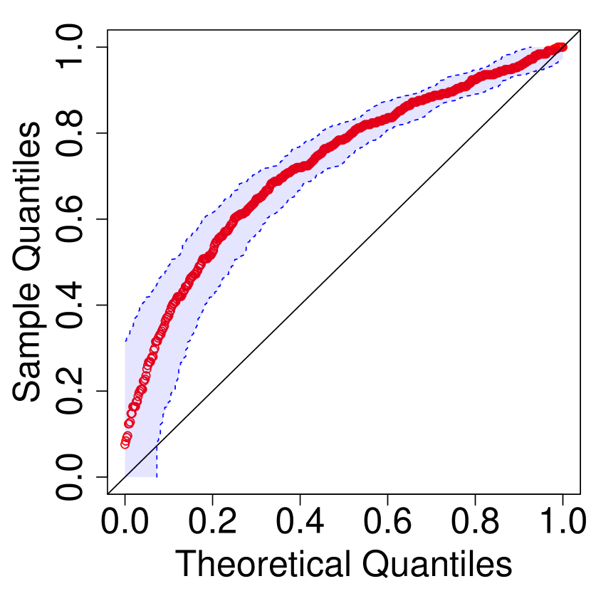
(b) $\mathcal{P}_{\beta}^{*}(0)$

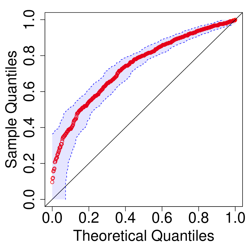
(c) $\mathcal{P}^{*}(0)$

(d) $\mathcal{P}_{\alpha,\beta}^{*}(4)$

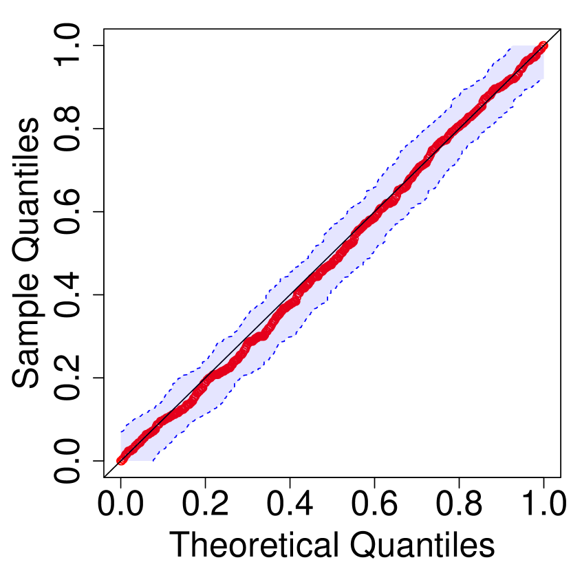
(e) $\mathcal{P}^{*}(4)$

Scenario 2: $\alpha_{S}=0.5$ and $\beta_{M}=0$.

By (a) and (b) of Figure 16, $\mathcal{P}_{\alpha}^{*}(0)$ and $\mathcal{P}_{\beta}^{*}(0)$ in Step 2 are conservative and non-conservative, respectively. This suggests that at least one of the true coefficients is non-zero. Thus, we can choose any $\lambda$ such that the double bootstrap yields estimated $p$-values similar to those in Step 2. The similarity between (d)–(e) and (a)–(b) indicates that $p$-values estimated by AB with $\lambda=2$ are similar to those in Step 2. This can be validated by comparing (c) and (f) of Figure 16, which show that increasing $\lambda$ to $2$ in AB still yields uniformly distributed $p$-values similar to those with $\lambda=0$.

Figure 15: Scenario 2: $\alpha_{S}=0.5$ and $\beta_{M}=0$.

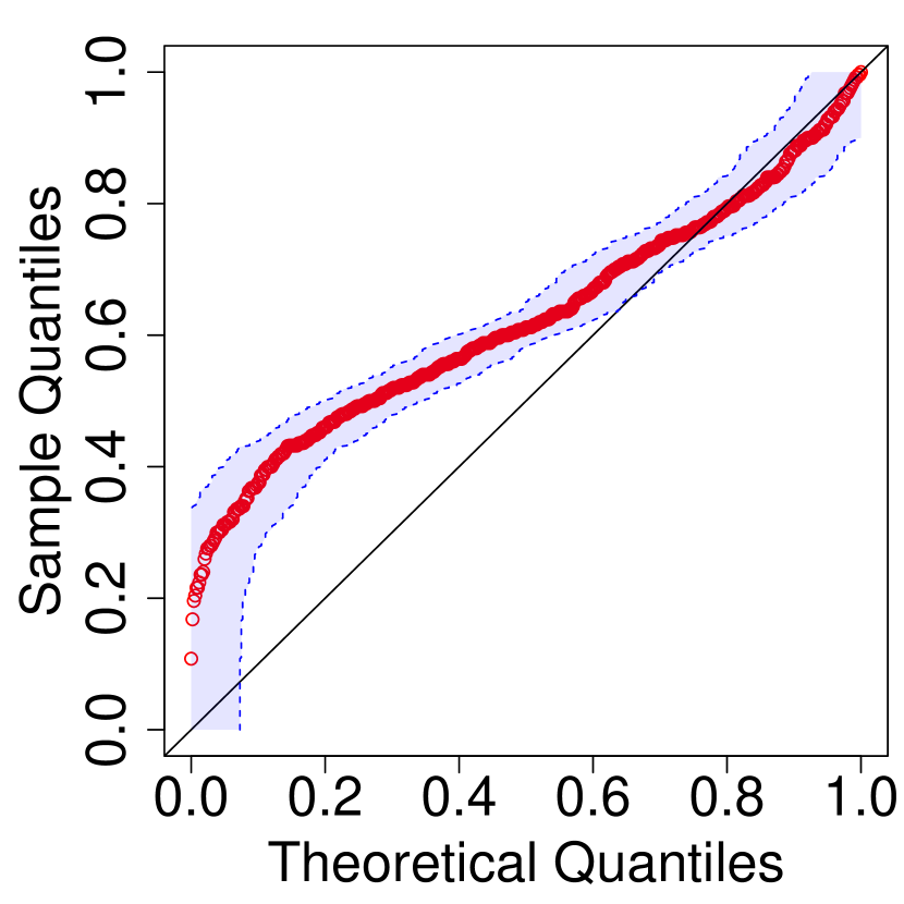
(a) $\mathcal{P}_{\alpha}^{*}(0)$

(b) $\mathcal{P}_{\beta}^{*}(0)$

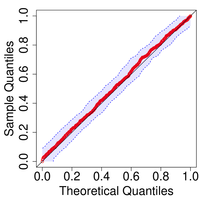
(c) $\mathcal{P}^{*}(0)$

(d) $\mathcal{P}_{\alpha}^{*}(2)$

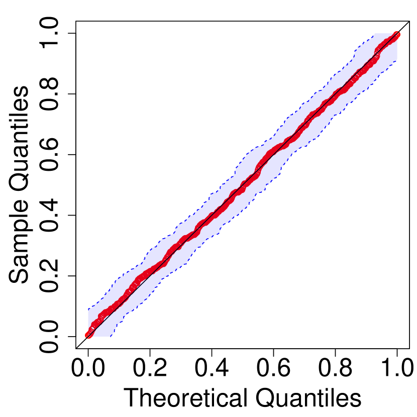
(e) $\mathcal{P}_{\beta}^{*}(2)$

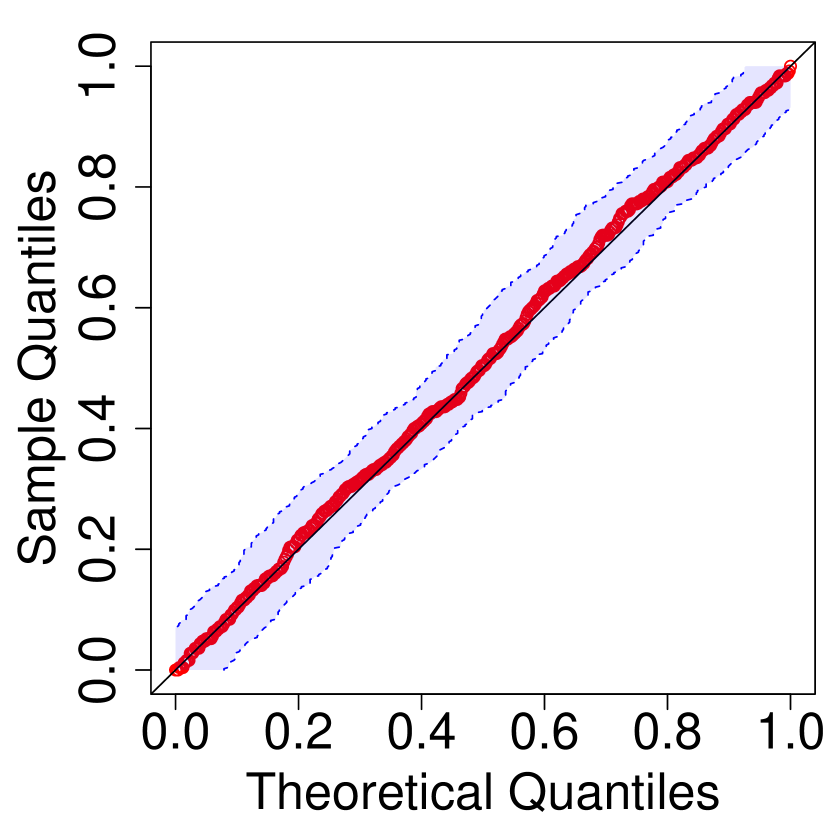
(f) $\mathcal{P}^{*}(2)$

Scenario 3: $\alpha_{S}=0$ and $\beta_{M}=0.5$.

The results are similar to those under Scenario 2, and similar analysis applies.

Figure 16: Scenario 3: $\alpha_{S}=0$ and $\beta_{M}=0.5$.

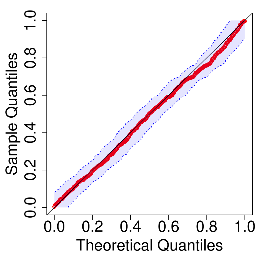
(a) $\mathcal{P}_{\alpha}^{*}(0)$

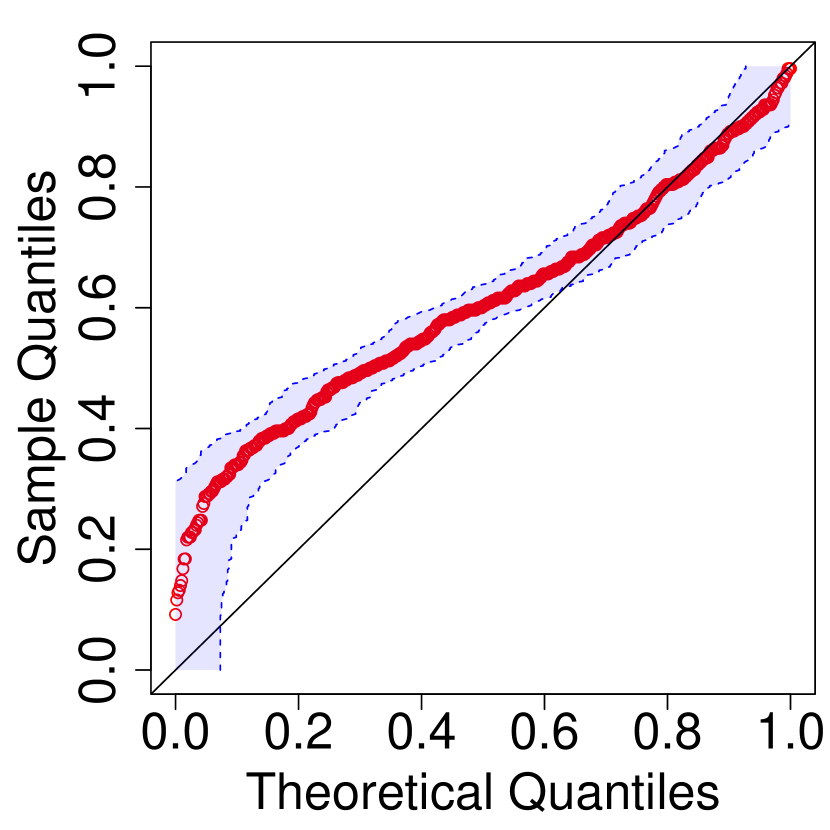
(b) $\mathcal{P}_{\beta}^{*}(0)$

(c) $\mathcal{P}^{*}(0)$

(d) $\mathcal{P}_{\alpha}^{*}(2)$

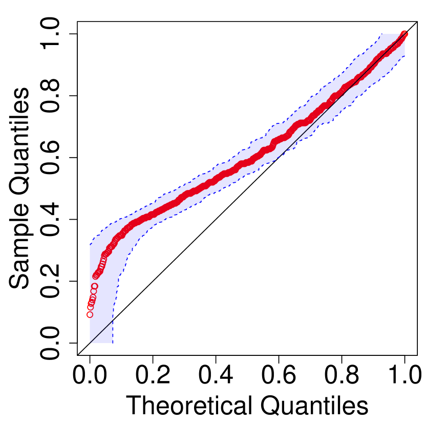
(e) $\mathcal{P}_{\beta}^{*}(2)$

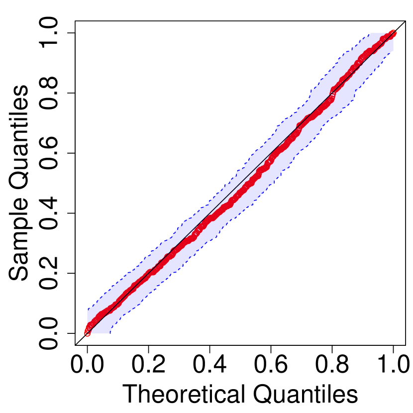
(f) $\mathcal{P}^{*}(2)$

F.2 Computation Facilitation: Projected Bootstrap

In this section, we propose a projected bootstrap procedure to facilitate the computation. In Theorem 2, we establish the bootstrap consistency results for $\hat{\alpha}_{S,n}^{*},$ $\hat{\beta}_{M,n}^{*},$ $\hat{\sigma}_{\alpha_{S},n}^{*},$ $\hat{\sigma}_{\beta_{M},n}^{*}$, and $\mathbb{R}_{n}^{*}(b_{\alpha},b_{\beta})$ that are computed from the nonparametric bootstrap, i.e., paired bootstrap in the regression settings. Particularly, for a bootstrapped index set $\mathcal{I}=\{k_{1},\ldots,k_{n}\}$, where $k_{j}\in\{1,\ldots,n\}$ for $j=1,\ldots,n$, the nonparametric bootstrap estimates are computed from the ordinary least squares regressions based on the bootstrapped data $\{(S_{i},\boldsymbol{X}_{i},M_{i},Y_{i}):i\in\mathcal{I}\}$. However, since the ordinary least squares regressions require matrix inversion, repeating this procedure for the structural equation models in each bootstrap can be computationally intensive.

Alternatively, inspired by the formulae in (28), we introduce a bootstrap procedure with a projection step to facilitate the computation. Specifically, we first compute the projected observations $\{(\hat{S}_{\perp,i},\hat{M}_{\perp,i},\hat{M}_{\perp^{\prime},i},\hat{Y}_{\perp^{\prime},i}):i=1,\ldots,n\}$ as defined in Section C.1. Then in the projected bootstrap procedure, with a bootstrapped index set $\mathcal{I}=\{k_{1},\ldots,k_{n}\}$, we compute the coefficients by

$$\hat{\alpha}_{S,\perp,n}^{*}=\frac{\sum_{i\in\mathcal{I}}\hat{S}_{\perp,i}\hat{M}_{\perp,i}}{\sum_{i\in\mathcal{I}}\hat{S}_{\perp,i}^{2}}=\frac{\mathbb{P}_{n}^{*}(\hat{S}_{\perp}\hat{M}_{\perp})}{\mathbb{P}_{n}^{*}(\hat{S}_{\perp}^{2})},\hskip 20.00003pt\hat{\beta}_{M,\perp^{\prime},n}^{*}=\frac{\sum_{i\in\mathcal{I}}\hat{M}_{\perp^{\prime},i}\hat{Y}_{\perp^{\prime},i}}{\sum_{i\in\mathcal{I}}\hat{M}_{\perp^{\prime},i}^{2}}=\frac{\mathbb{P}_{n}^{*}(\hat{M}_{\perp^{\prime}}\hat{Y}_{\perp^{\prime}})}{\mathbb{P}_{n}^{*}(\hat{M}_{\perp^{\prime}}^{2})},$$

and obtain the residuals by $\hat{\epsilon}_{M,\perp,n,i}=\hat{M}_{\perp,i}-\hat{S}_{\perp,i}\hat{\alpha}_{S,\perp,n}$ and $\hat{\epsilon}_{Y,\perp^{\prime},n,i}=\hat{Y}_{\perp^{\prime},i}-\hat{M}_{\perp^{\prime},i}\hat{\beta}_{M,\perp^{\prime},n}$ for $i\in\mathcal{I}$. Moreover, we define

$$(\hat{\sigma}_{\alpha_{S},\perp,n}^{*})^{2}= {\sum_{i\in\mathcal{I}}\hat{\epsilon}_{M,\perp,n,i}^{2}}/{n},\ \mathbb{V}_{S,\perp,n}^{*}= \sum_{i\in\mathcal{I}}\hat{S}_{\perp,i}^{2}/n,\ \mathbb{Z}_{S,\perp,n}^{*}= \sum_{i\in\mathcal{I}}\hat{\epsilon}_{M,\perp,n,i}\hat{S}_{\perp,i}/n,$$

$$(\hat{\sigma}_{\beta_{M},\perp^{\prime},n}^{*})^{2}= {\sum_{i\in\mathcal{I}}\hat{\epsilon}_{Y,\perp^{\prime},n,i}^{2}}/{n},\ \mathbb{V}_{M,\perp^{\prime},n}^{*}= \sum_{i\in\mathcal{I}}\hat{M}_{\perp^{\prime},i}^{2}/n,\ \mathbb{Z}_{M,\perp^{\prime},n}^{*}= \sum_{i\in\mathcal{I}}\hat{\epsilon}_{Y,\perp^{\prime},n,i}\hat{M}_{\perp^{\prime},i}/n,$$

which can be viewed as projected bootstrap versions of $\hat{\sigma}_{\alpha_{S},n}^{*}$, $\hat{\sigma}_{\beta_{M},n}^{*}$, $\mathbb{Z}_{S,n}^{*}$, $\mathbb{Z}_{M,n}^{*}$, $\mathbb{V}_{S,n}^{*}$, and $\mathbb{V}_{M,n}^{*}$, respectively, where we replace $(\hat{\epsilon}_{M,n},\hat{\epsilon}_{Y,n},S_{\perp}^{*},M_{\perp^{\prime}}^{*})$ with $(\hat{\epsilon}_{M,\perp,n},\hat{\epsilon}_{Y,\perp^{\prime},n},\hat{S}_{\perp},\hat{M}_{\perp^{\prime}})$.

In the proposed projected bootstrap, matrix inversion is only required in the projection step, and not repeated. Therefore, the computational cost can be significantly reduced. Theoretically, we can prove the following Lemma F.25, and then by Slutsky’s lemma, the bootstrap consistency results in Theorems 2 and 12 still hold for the projected bootstrap procedure. The proof of Lemma F.25 is given in Section C.6.3.

Lemma F.25.

Under Condition 1,

1. $\sqrt{n}(\hat{\alpha}_{S,n}^{*}-\hat{\alpha}_{S,\perp,n}^{*})\overset{\mathrm{P}^{*}}{\leadsto}0$ and $\sqrt{n}(\hat{\beta}_{M,n}^{*}-\hat{\beta}_{M,\perp^{\prime},n}^{*})\overset{\mathrm{P}^{*}}{\leadsto}0$;

2. $\mathbb{Z}_{S,n}^{*}-\mathbb{Z}_{S,\perp,n}^{*}\overset{\mathrm{P}^{*}}{\leadsto}0$ and $\mathbb{Z}_{M,n}^{*}-\mathbb{Z}_{M,\perp^{\prime},n}^{*}\overset{\mathrm{P}^{*}}{\leadsto}0$;

3. $\mathbb{V}_{S,n}^{*}-\mathbb{V}_{S,\perp,n}^{*}\overset{\mathrm{P}^{*}}{\leadsto}0$ and $\mathbb{V}_{M,n}^{*}-\mathbb{V}_{M,\perp^{\prime},n}^{*}\overset{\mathrm{P}^{*}}{\leadsto}0$;

4. $(\hat{\sigma}_{\alpha_{S},n}^{*})^{2}-(\hat{\sigma}_{\alpha_{S},\perp,n}^{*})^{2}\overset{\mathrm{P}^{*}}{\leadsto}0$ and $(\hat{\sigma}_{\beta_{M},n}^{*})^{2}-(\hat{\sigma}_{\beta_{M},\perp^{\prime},n}^{*})^{2}\overset{\mathrm{P}^{*}}{\leadsto}0$.

Appendix G Additional Numerical Results

In this section, Section G.1 presents figures supplementary to Section 4.1 in the main text. Section G.2 presents additional simulation experiments examining the effects of varying signal sizes and sample sizes. Section G.3 presents additional data analysis results including marginal screening, the joint testing, a sensitivity analysis, interpretation of data analysis results, and a confirmatory analysis,.

G.1 QQ-Plots Supplementary to Section 4.1

Figure 17: Q-Q plots of $p$-values under the fixed null with $n=500$.

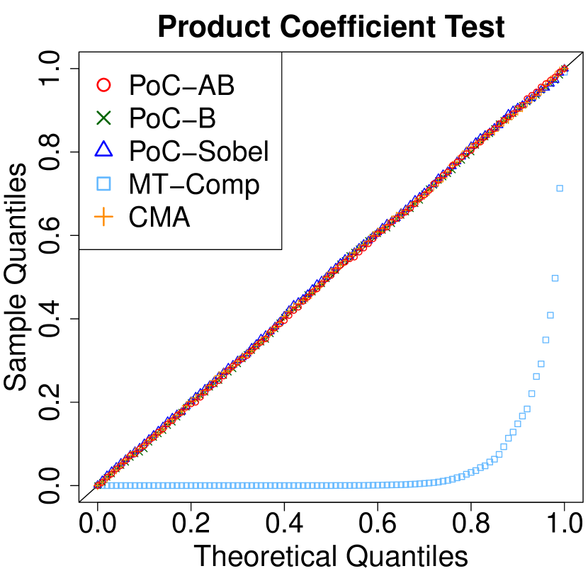
(a)    $H_{0,1}:(\alpha_{S},\beta_{M})=(0,0.5)$

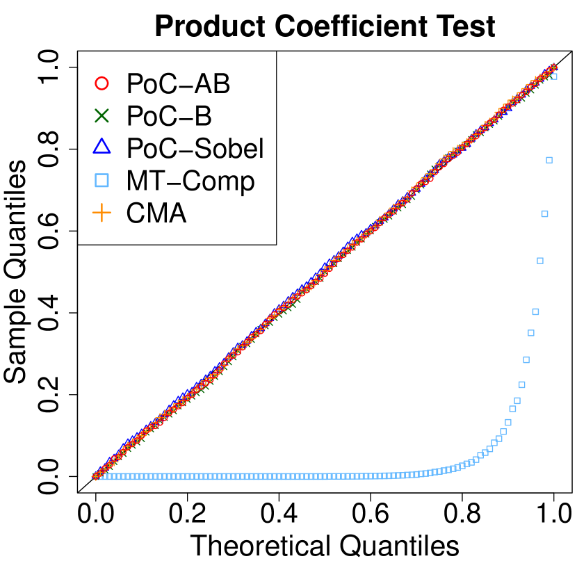
(b)    $H_{0,2}:(\alpha_{S},\beta_{M})=(0.5,0)$

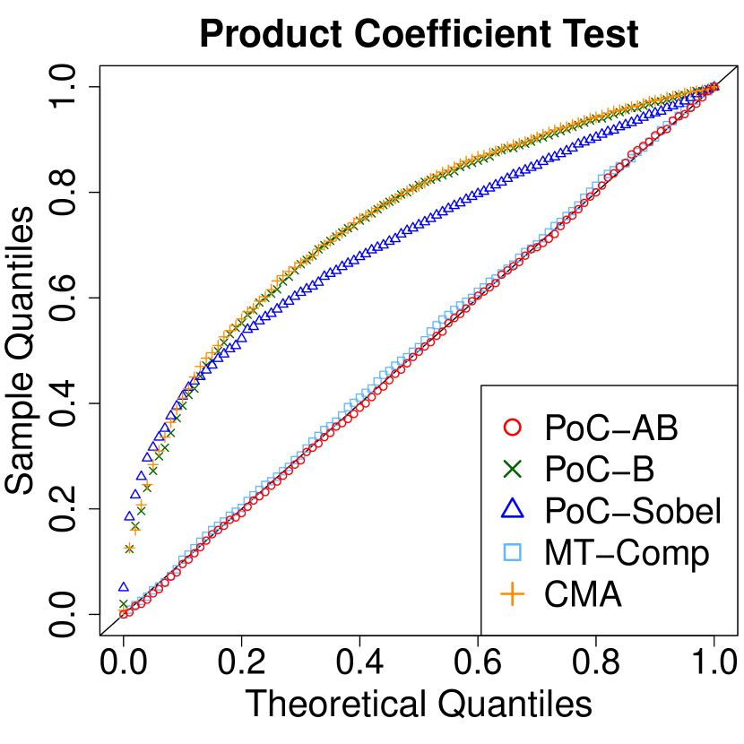
(c)    $H_{0,3}:(\alpha_{S},\beta_{M})=(0,0)$

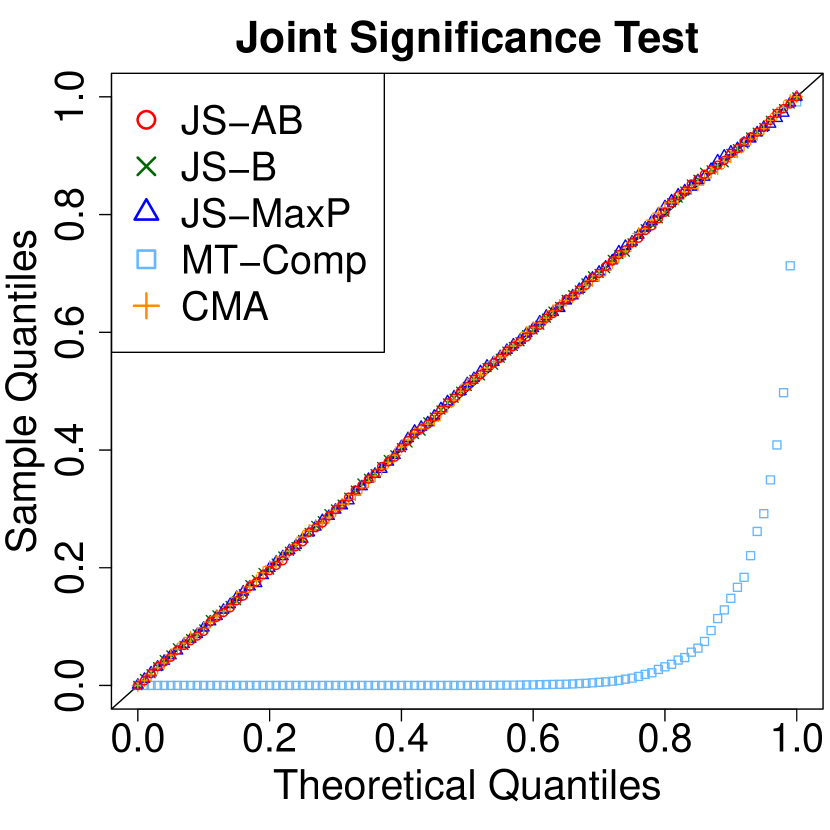
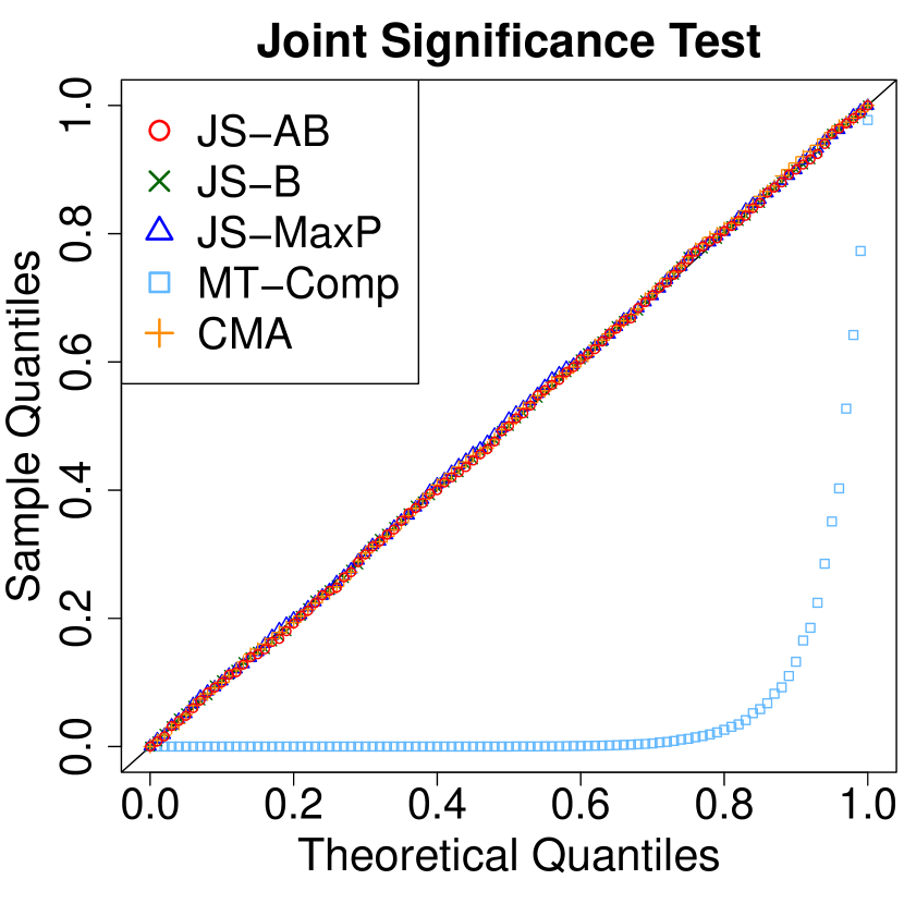
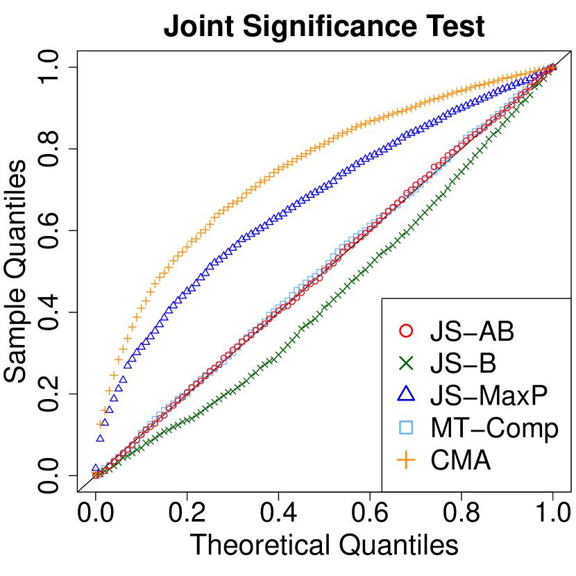
Figure 18: Q-Q plots of $p$-values under the mixture of nulls: $n=500$.

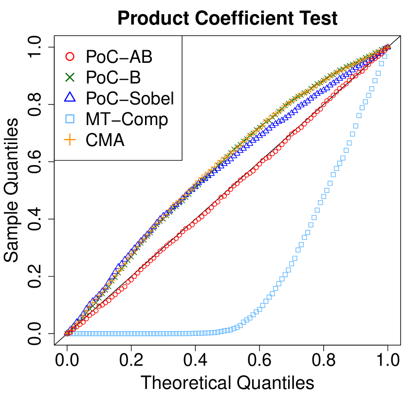
(a)    (I) $(1/3,1/3,1/3)$

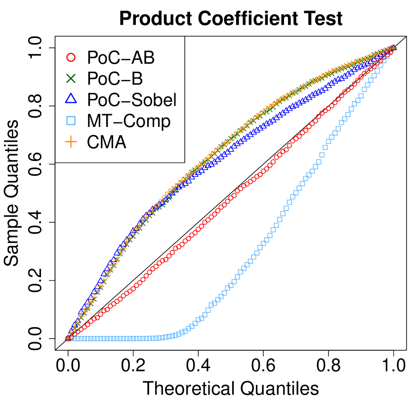
(b)    (II) $(0.2,0.2,0.6)$

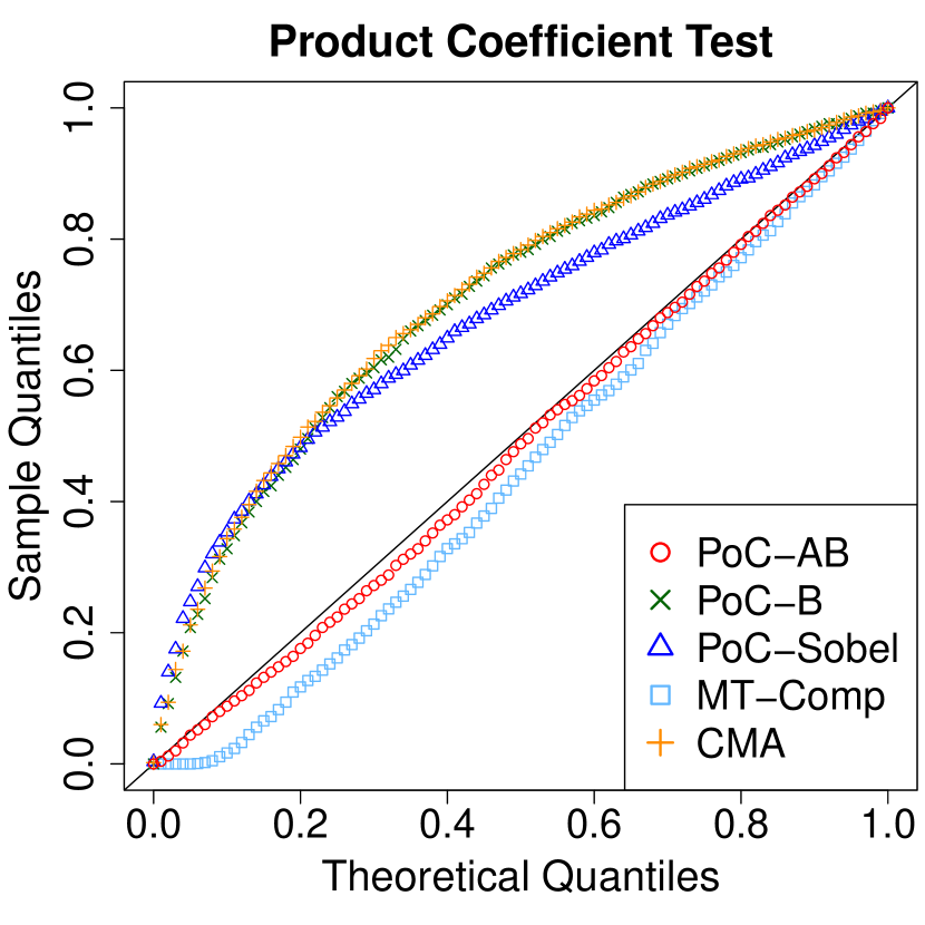
(c)    (III) $(0.05,0.05,0.9)$

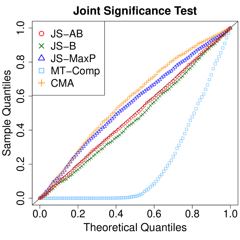
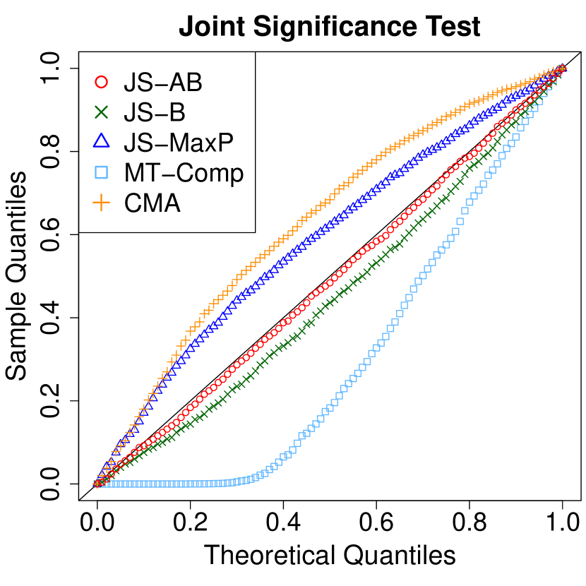
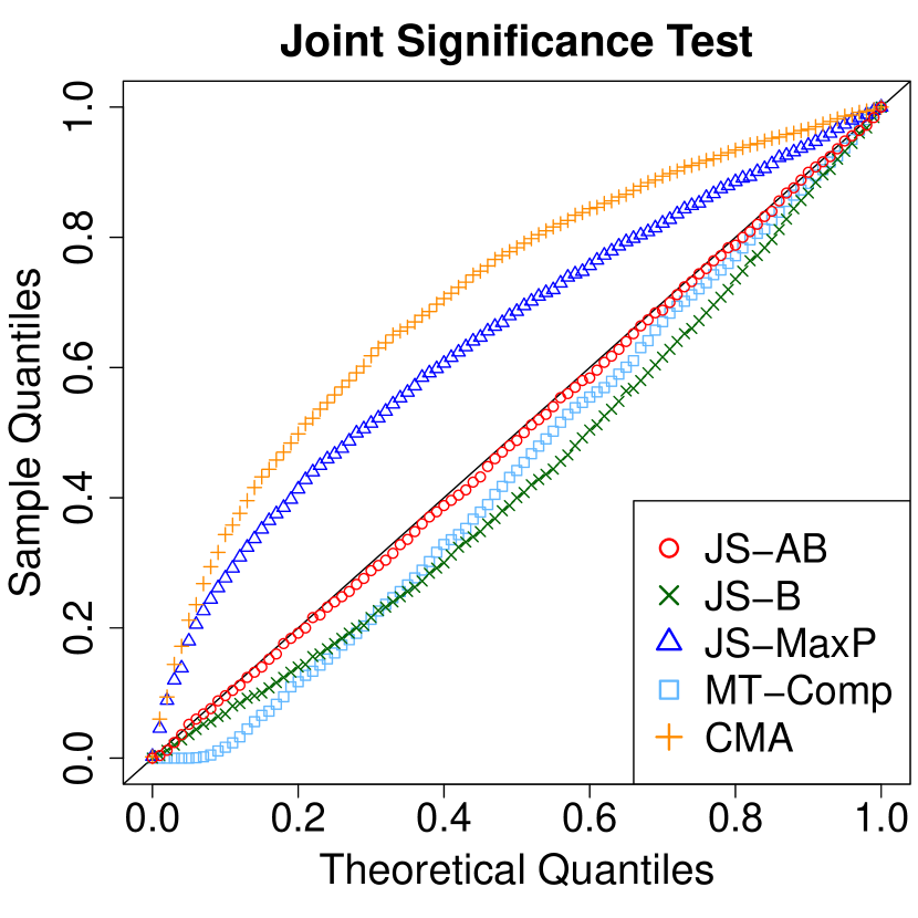
G.2 Additional Simulations: Varying Effects and Sample Sizes

We illustrate how the proposed method performs in terms of the type-I error control when the effect sizes and sample sizes become larger. In particular, we generate data following the model $M=\alpha_{S}S+\alpha_{I}+\epsilon_{M},$ and $Y=\beta_{M}M+\beta_{I}+S+\epsilon_{Y}$, where the exposure variable $S$ is simulated from a Bernoulli distribution with the success probability equal to 0.5, and $\epsilon_{M}$ and $\epsilon_{Y}$ are simulated independently from $\mathcal{N}(0,\sigma^{2})$ with $\sigma=0.5$. To evaluate how the varying effect sizes and sample sizes influence the type-I errors, we consider two cases under $H_{0}$: $\alpha_{S}\beta_{M}=0$:

1. Fix $\alpha_{S}=0$, take $\beta_{M}=\exp(k)$ for $k\in\{-\infty,0,1,2,3,4,5\}$.

2. Fix $\beta_{M}=0$, take $\alpha_{S}=\exp(k)$ for $k\in\{-\infty,0,1,2,3,4,5\}$.

Estimated type-I errors of different tests under cases (i) and (ii) are presented in Figures 19 and 20, respectively. We can see that the AB tests control the type-I errors well under different values of the non-zero coefficients, whereas the other tests can deviate from the nominal significance level when both coefficients are 0.

Figure 19: When $\alpha_{S}=0$, estimated type-I errors

(a) PoC-tests with significance level 0.05

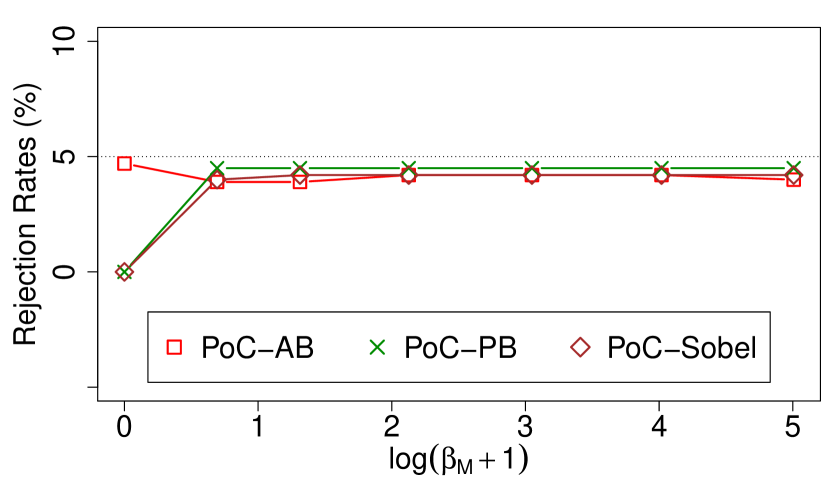
(a) (a.1) $n=200$

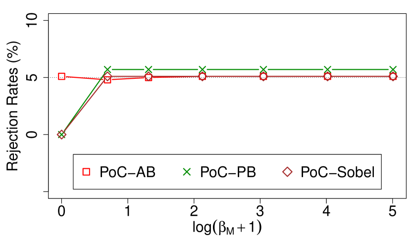
(b) (a.2) $n=500$

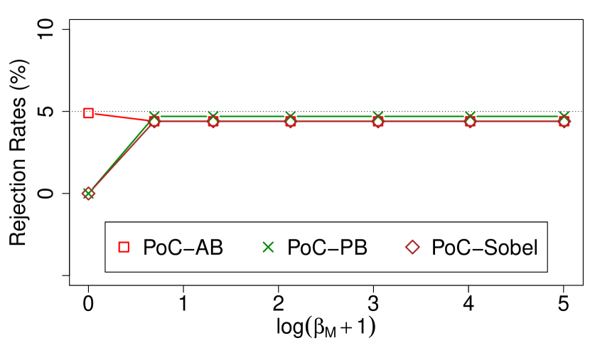
(c) (a.3) $n=1000$

(b) PoC-tests with significance level 0.1

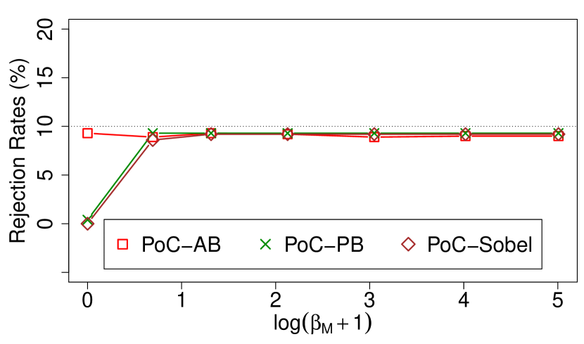
(d) (b.1) $n=200$

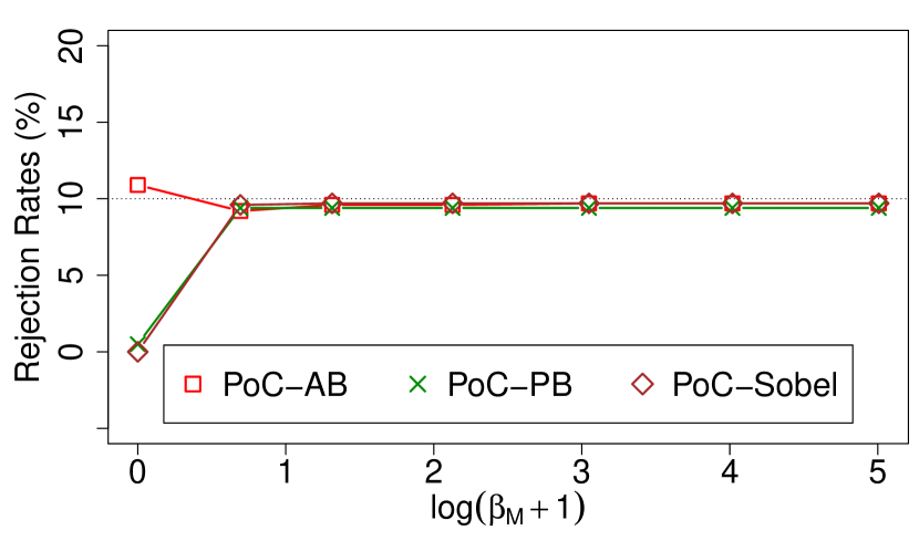
(e) (b.2) $n=500$

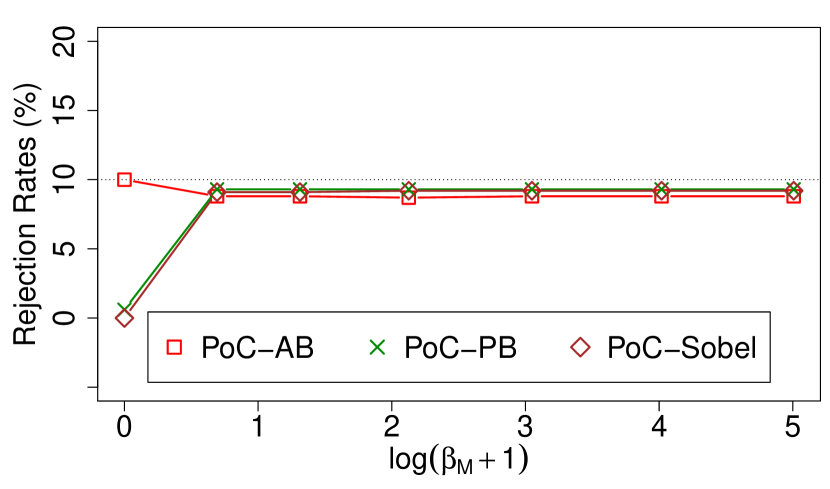
(f) (b.3) $n=1000$

(c) JS-tests with significance level $0.05$

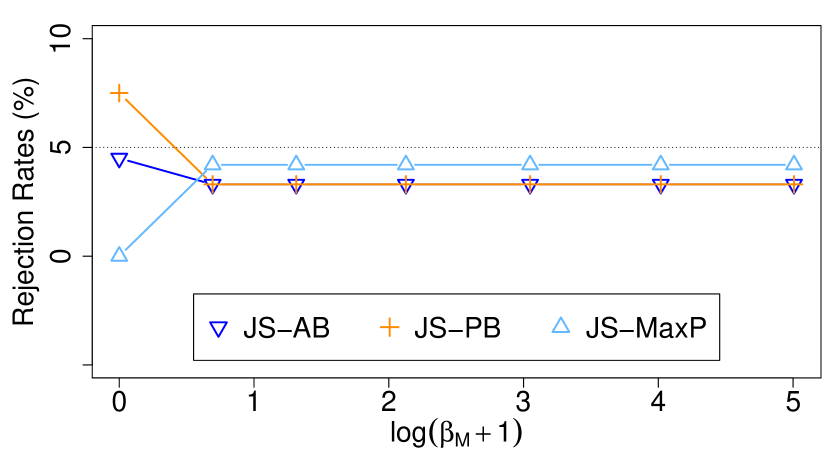
(g) (c.1) $n=200$

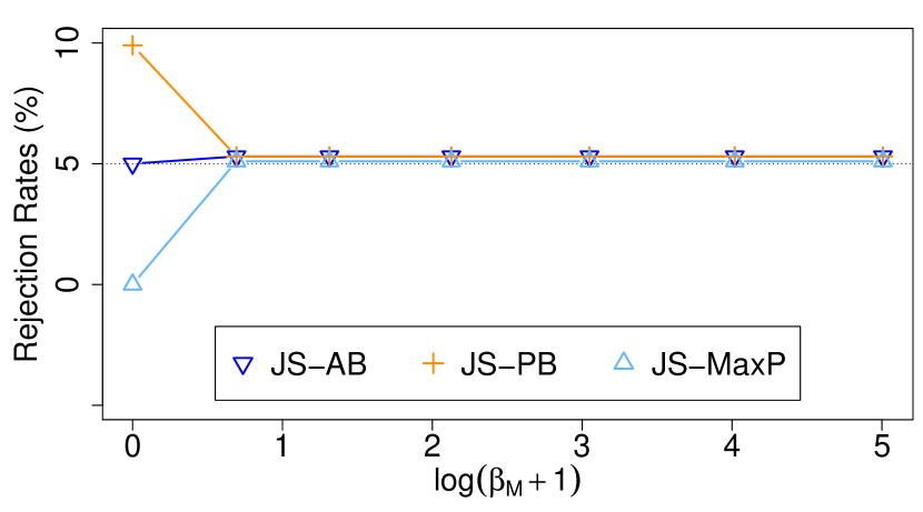
(h) (c.2) $n=500$

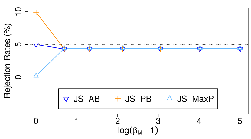
(i) (c.3) $n=1000$

(d) JS-tests with significance level $0.05$

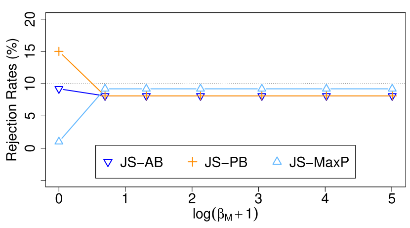
(j) (d.1) $n=200$

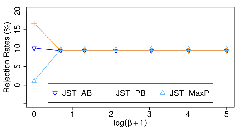
(k) (d.2) $n=500$

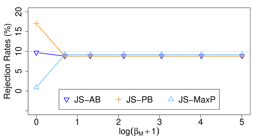
(l) (d.3) $n=1000$

Figure 20: When $\beta_{M}=0$, estimated type-I errors

(a) PoC-tests with significance level 0.05

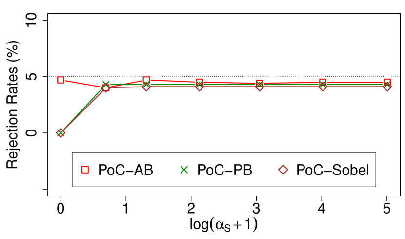
(a) (a.1) $n=200$

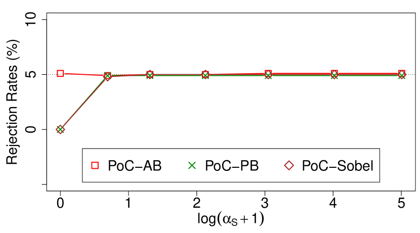
(b) (a.2) $n=500$

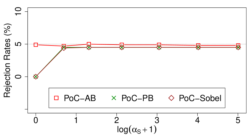
(c) (a.3) $n=1000$

(b) PoC-tests with significance level 0.1

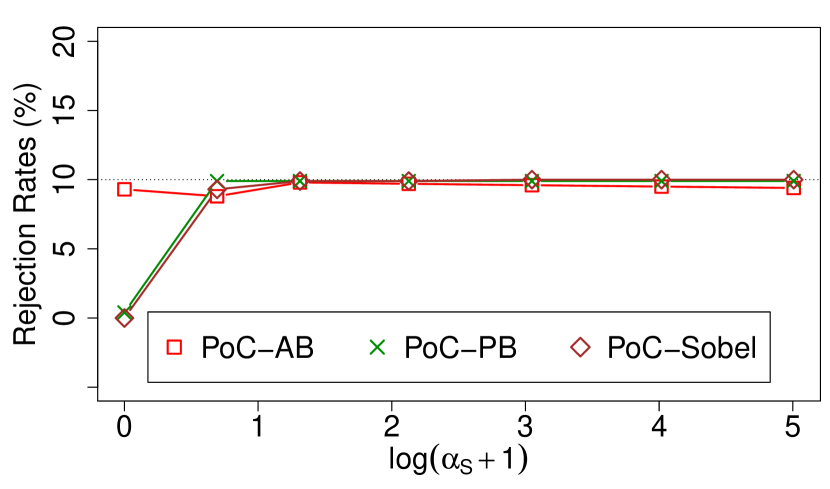
(d) (b.1) $n=200$

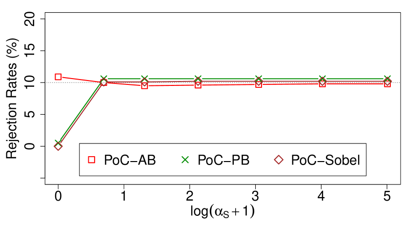
(e) (b.2) $n=500$

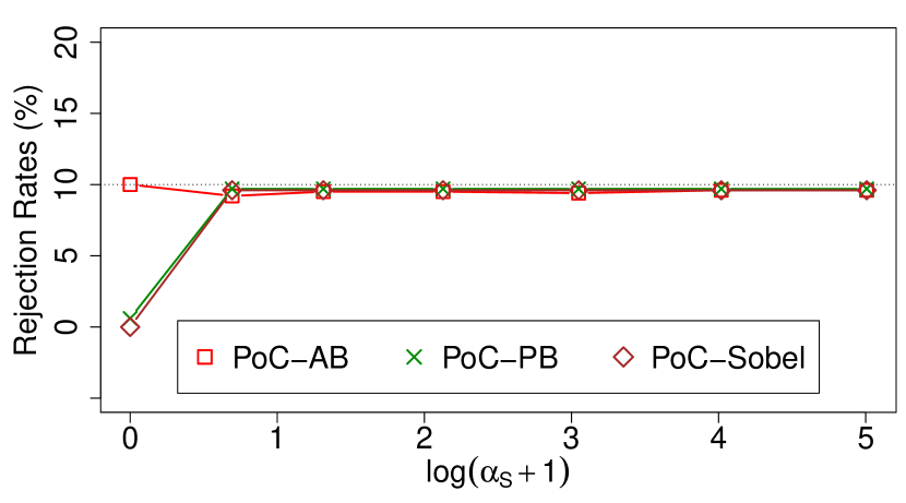
(f) (b.3) $n=1000$

(c) JS-tests with significance level $0.05$

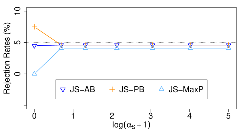
(g) (c.1) $n=200$

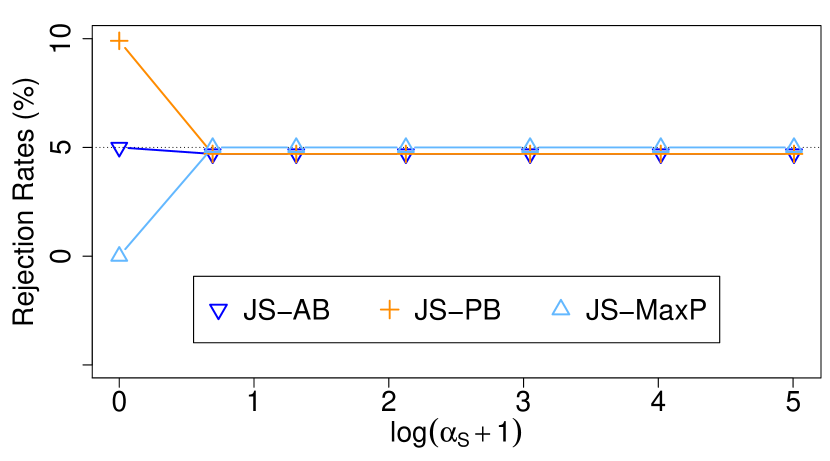
(h) (c.2) $n=500$

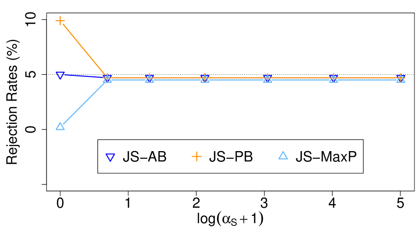
(i) (c.3) $n=1000$

(d) JS-tests with significance level $0.1$

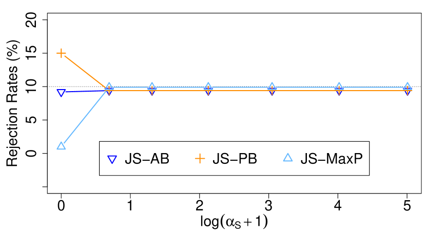
(j) (d.1) $n=200$

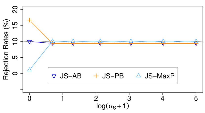
(k) (d.2) $n=500$

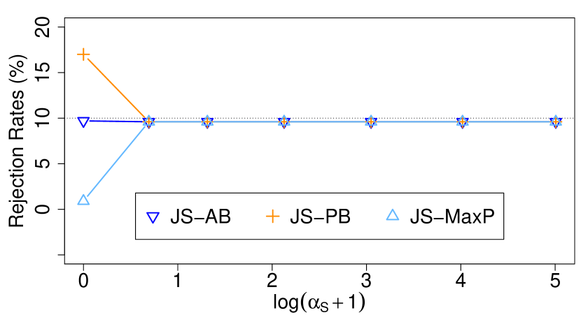
(l) (d.3) $n=1000$

G.3 Data Analysis: Supplementary Results

G.3.1 Additional Two-Step Data Analysis Results

In Section 6, we conducted a two-step data analysis by retaining 10% of lipids with the smallest $p$-values in the first step. In the following, we extend our analysis by varying the proportion ($q\%$) of lipids retained in the first step. Figures 21–25 present the results when $q\in\{5,10,15,20,25\}$, corresponding to 8, 15, 22, 30, and 38 lipids with the smallest $p$-values retained after the initial screening. Each figure showcases the top five mediators most frequently selected over 400 random splits and six tests. Notably, regardless of the screening percentage, L.A and FA.7 consistently emerge as the most frequently selected mediators. This suggests that our results are robust to the specific choice of screening threshold used in the first step.

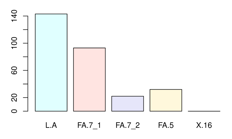
(a) JS-AB

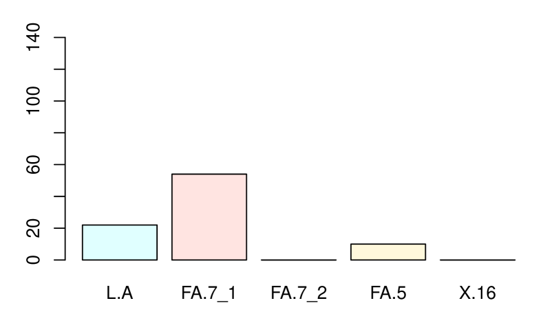
(b) JS-MaxP

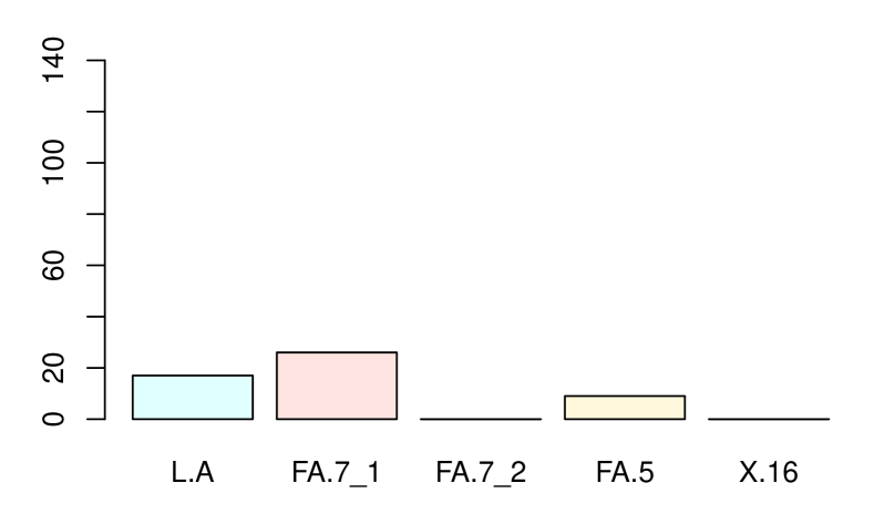
(c) CMA

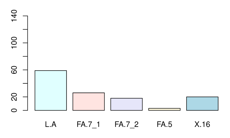
(d) PoC-AB

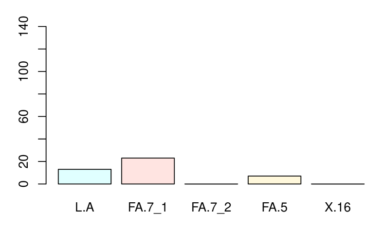
(e) PoC-B

(f) PoC-Sobel

Figure 21: Times of mediators being selected in Step 2 by the six tests when FDR$=0.10$ over 400 random splits of the data. Keep 5% of lipids with the smallest $p$-values in Step 1. (Abbreviations: LAURIC.ACID (L.A); FA.7.0-OH_1 (FA.7_1); FA.5.0-OH (FA.5); FA.7.0-OH_2 (FA.7_2); X16.0.LYSO.PC_2 (X.16).

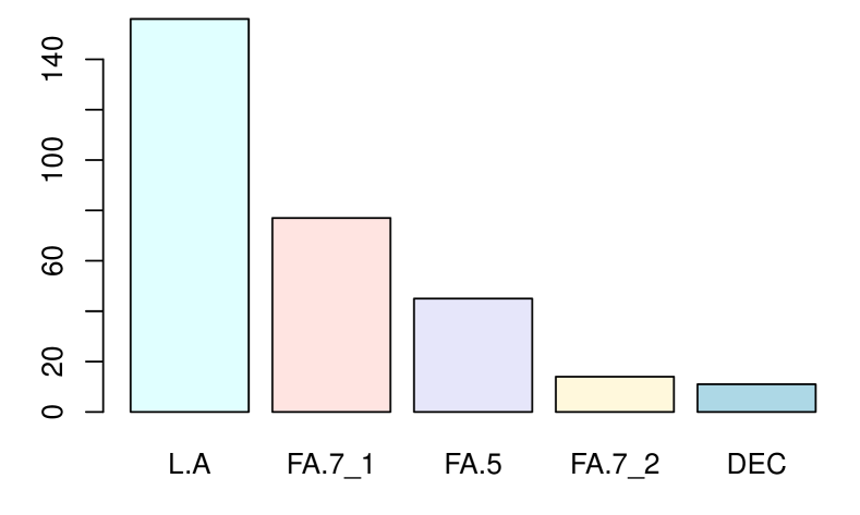
(a) JS-AB

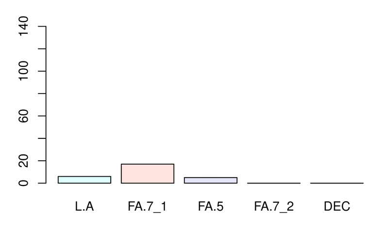
(b) JS-MaxP

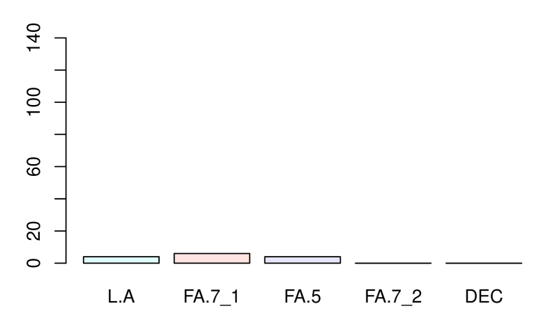
(c) CMA

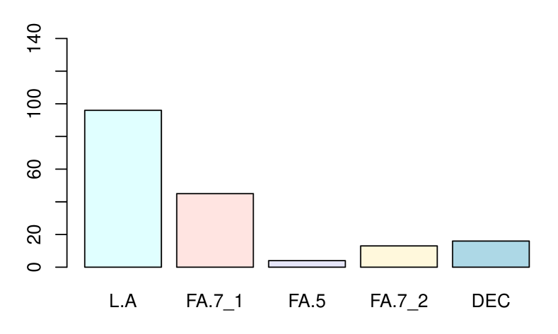
(d) PoC-AB

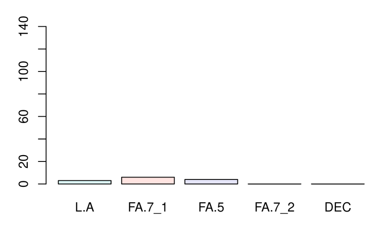
(e) PoC-B

(f) PoC-Sobel

Figure 22: Times of mediators being selected in Step 2 by the six tests when FDR$=0.10$ over 400 random splits of the data. Keep 10% of lipids with the smallest $p$-values in Step 1. (Abbreviations: LAURIC.ACID (L.A); FA.7.0-OH_1 (FA.7_1); FA.5.0-OH (FA.5); FA.7.0-OH_2 (FA.7_2); DECENOYLCARNITINE (DEC).

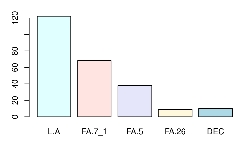
(a) JS-AB

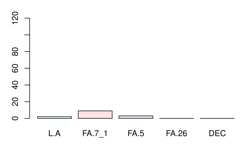
(b) JS-MaxP

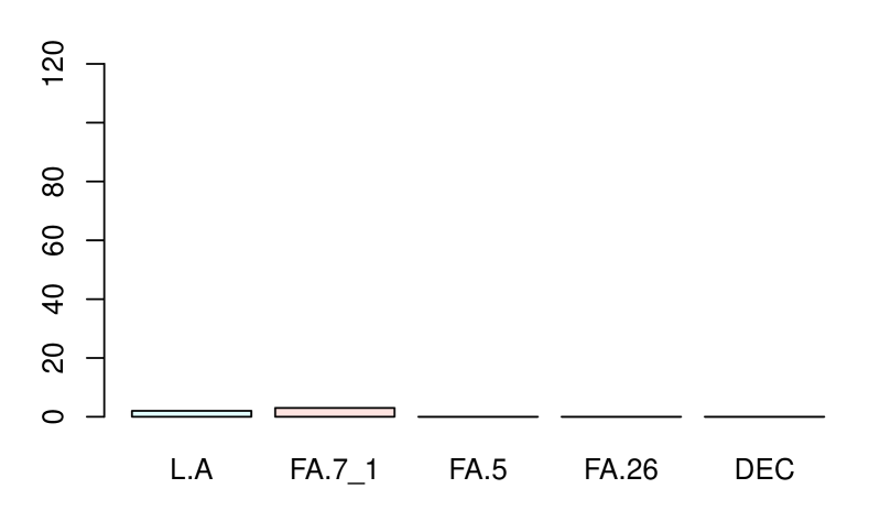
(c) CMA

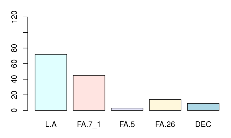
(d) PoC-AB

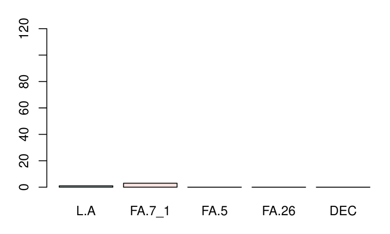
(e) PoC-B

(f) PoC-Sobel

Figure 23: Times of mediators being selected in Step 2 by the six tests when FDR$=0.10$ over 400 random splits of the data. Keep 15% of lipids with the smallest $p$-values in Step 1. (Abbreviations: LAURIC.ACID (L.A); FA.7.0-OH_1 (FA.7_1); FA.5.0-OH (FA.5); FA.26 (FA.26.0-OH); DECENOYLCARNITINE (DEC).

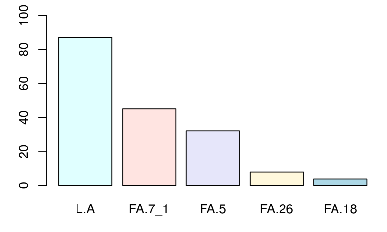
(a) JS-AB

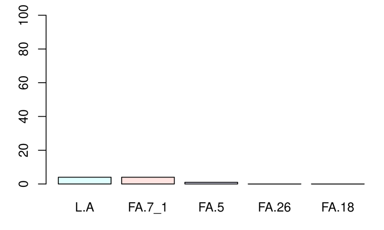
(b) JS-MaxP

(c) CMA

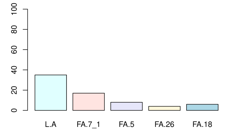
(d) PoC-AB

(e) PoC-B

(f) PoC-Sobel

Figure 24: Times of mediators being selected in Step 2 by the six tests when FDR$=0.10$ over 400 random splits of the data. Keep 20% of lipids with the smallest $p$-values in Step 1. (Abbreviations: LAURIC.ACID (L.A); FA.7.0-OH_1 (FA.7_1); FA.5.0-OH (FA.5); FA.26 (FA.26.0-OH); FA.18 (FA.18.1_2).

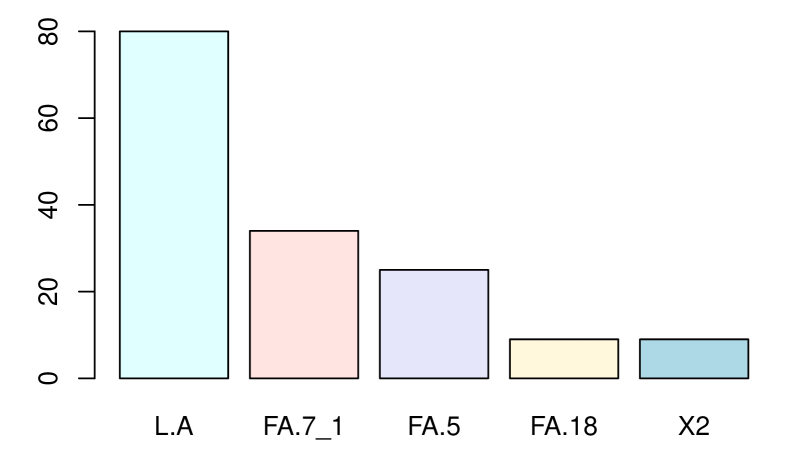
(a) JS-AB

(b) JS-MaxP

(c) CMA

(d) PoC-AB

(e) PoC-B

(f) PoC-Sobel

Figure 25: Times of mediators being selected in Step 2 by the six tests when FDR$=0.10$ over 400 random splits of the data. Keep 25% of lipids with the smallest $p$-values in Step 1. (Abbreviations: LAURIC.ACID (L.A); FA.7.0-OH_1 (FA.7_1); FA.5.0-OH (FA.5); FA.18 (FA.18.1_2); X.2 (X2.OCTENOYLCARNITINE.CAT).

G.3.2 Testing the Joint Mediation Effect

We evaluate the joint mediation effect following the discussions in Section 5.1. Similarly to Section 6, we first apply a screening analysis to identify a subset of lipids as potential candidates, and then test the joint mediation effect of the chosen lipids in the second step. To prevent potential issues arising from double dipping the data, we randomly split the data into two parts, which are used in the two steps, respectively. Besides the joint AB test in Section 5.1, we also include three existing approaches to testing the group-level mediation effect: Product Test based on Normal Product distribution (PT-NP) (Huang and Pan, 2016) Product Test based on Normality (PT-N) (Huang and Pan, 2016), and the Simultaneous Likelihood Ratio (SLR) Test in Hao and Song (2022).

Table 3 presents $p$-values of the four tests under a single random split, as an illustrative example. The proposed AB test returns the most significant $p$-value, and it rejects the null hypothesis of no joint mediation effect at the 0.05 significance level. We further replicate the two-step analysis by randomly splitting the data 400 times. For each test, Figure 26 presents a histogram of 400 $p$-values obtained from 400 random splits. All the four histograms are right skewed. The AB test shows a higher chance of yielding smaller $p$-values compared the other existing tests. This aligns with our observation that the AB test achieves high statistical power in simulations in Section D.2.4.

Table 3: Results of testing the joint mediation effect after the first screening step.

tests	AB Test	PT-N	PT-NP	SLR
$p$-values	0.0166	0.0856	0.1020	0.0726

(a) AB Test

(b) PT-N

(c) PT-NP

(d) SLR

Figure 26: Histogram of p-values of testing joint mediation effect in Step 2.

G.3.3 Data Analysis: Interpretation of Results in the Second Step

In the second step of the data analysis, let $\{\text{lipid}_{j}:j=1,\ldots,15\}$ denote the selected lipids of interest. Our analysis considers the linear and additive mean regression model:

$$\operatorname{BMI}\sim ~{}\sum_{j=1}^{15}\beta_{j}\operatorname{lipid}_{j}+\tau\operatorname{Exposure}+\boldsymbol{X}^{\top}\beta_{X},$$ (62)

$$\operatorname{lipid}_{j}\sim ~{}\alpha_{j}\operatorname{Exposure}+\boldsymbol{X}^{\top}\alpha_{X,j},\quad\quad\text{for }j=1,\ldots,15,$$

where $\boldsymbol{X}=(1,\text{age},\text{gender})^{\top}$ denotes the baseline covariates. For one candidate lipid of interest, say, lipid₁, we test $H_{0}:\alpha_{1}\beta_{1}=0$ in the above multivariate structural equation model (62). This hypothesis pertains to two possible causal paths for interpretation along with the discussion on Page 3 of the main text. First, if the mediators follow the parallel path model in Section D.1.1, the individual mediation path $\text{Exposure}\to\text{lipid}_{1}\to\text{BMI}$ can be identified. In this case, rejecting $H_{0}:\alpha_{1}\beta_{1}=0$ indicates that there exists a mediation effect through the path $\text{Exposure}\to\text{lipid}_{1}\to\text{BMI}$. Second, if lipid₁ is is causally correlated with other lipids, according to Section D.1.2, the coefficients-product $\alpha_{1}\beta_{1}$ may be interpreted as the interventional indirect effect, which is the combined mediation effects along all (unknown) causal pathways via $\text{lipid}_{1}$ as well as any other lipids that causally precede $\text{lipid}_{1}$. Also see Section D.1 for a detailed introduction on the two scenarios. Given the fact that these lipids are in the same biological pathway and highly likely to be causally related, we are inclined to draw conclusion of our analysis using the second interpretation, namely the interventional indirect effect.

G.3.4 Sensitivity Analysis

Recall that the screening step in Section 6 considers one mediator at a time in the outcome model. We conduct sensitivity analyses to evaluate the effects of unadjusted mediators (Imai et al., 2010b; Liu et al., 2021). The first-step estimates are identified if the sequential ignorability assumption in Section 2 holds. Imai et al. (2010b) proposed to use the correlation between the error terms in the Y-M model and the M-S model as a sensitivity parameter. As an instance, when only considering one mediator $M_{j}$, we can equivalently rewrite outcome model in (13) as $Y=\beta_{M,j}M_{j}+\boldsymbol{X}^{\top}\boldsymbol{\beta}_{\boldsymbol{X}}+\tau_{S}S+\epsilon_{Y,j}$, where $\epsilon_{Y,j}=\sum_{k\neq j}\beta_{M,k}M_{k}+\epsilon_{Y}$. When the sequential ignorability assumption is violated, the correlation $\rho_{j}=\mathrm{corr}(\epsilon_{Y,j},\epsilon_{M,j})$ is likely to be nonzero, and vice versa. Following Imai et al. (2010b), we hypothetically vary the value of $\rho_{j}$ and compute the corresponding estimate of the mediation effect. When $|\rho_{j}|$ deviates from 0 to certain value, the obtained mediation effects could be explained away by the bias from unadjusted mediators. For each tested mediator $M_{j}$, we compute the minimum value of $|\rho_{j}|$ such that the observed mediation effect becomes 0 through the R package mediation (Tingley et al., 2014).

Table 4 presents the sensitivity analysis results for the mediators with absolute mediation effects greater than 0.05. We discuss the results of the mediator LAURIC.ACID as an example. Table 4 suggests that the bias from the correlation between the two error terms $\mathrm{corr}(\epsilon_{M,j},\epsilon_{Y})$ needs to be at least 0.16 such that the mediation effect becomes 0. On the other hand, the sample correlation between the two residual terms is -4.83e-17, which is much smaller than $\rho_{\min}=0.16$. This suggests that the bias from error correlation could be negligible. Similarly for other selected mediators, the residual correlation are very close to zero and much smaller than the corresponding confounding bias measured $\rho_{\min}$. Therefore, the sensitivity analysis results show that mediation analysis results for this ELEMENT dataset can be robust to the bias from the potential error correlation.

Table 4: Sensitivity analysis of selected mediators in the ELEMENT study. ME represents estimated mediation effects. $\hat{\alpha}$ and $\hat{\beta}$ represent samples estimates of $\alpha_{S}$ and $\beta_{M}$, respectively. $p_{\alpha}$ and $p_{\beta}$ represent the $p$-values of coefficients $\alpha_{S}$ and $\beta_{M}$, respectively. $\rho_{\min}$ represents the bias measured by $\mathrm{corr}(\epsilon_{M},\epsilon_{Y})$ at which NIE$=0$, where we use 0.01 increment. $\hat{\rho}$ stands for sample Pearson’s correlation between two error terms $\epsilon_{M}$ and $\epsilon_{Y}$.

	ME	$\hat{\alpha}$	$p_{\alpha}$	$\hat{\beta}$	$p_{\beta}$	$\rho_{min}$	$\hat{\rho}$
FA 7:0-OH._1	0.18	0.20	0.00	0.87	0.00	0.21	4.59e-17
FA 7:0-OH._2	0.12	0.15	0.00	0.82	0.00	0.20	1.86e-17
LPC 16:1_3	0.06	0.18	0.00	0.32	0.13	0.08	-1.27e-17
LPC 18:2_2	0.05	0.17	0.00	0.31	0.14	0.08	3.91e-17
LPC 18:3_1	0.06	0.11	0.02	0.57	0.01	0.13	7.70e-17
X10.HYDRO-H2O	-0.08	0.26	0.00	-0.30	0.16	-0.07	-7.91e-18
DECENOYL	-0.05	0.14	0.01	-0.38	0.07	-0.09	-1.00e-17
FA 18:0-DiC.	-0.05	0.14	0.01	-0.37	0.07	-0.09	1.18e-16
FA 5:0-OH.	0.11	0.09	0.08	1.20	0.00	0.30	9.11e-18
GLY	0.06	0.12	0.02	0.50	0.02	0.12	1.26e-16
GLY-H2O	0.06	0.15	0.00	0.44	0.04	0.11	-3.99e-17
LAURIC.ACID	0.14	0.21	0.00	0.66	0.00	0.16	-4.83e-17

G.3.5 Volcano Plots in the Screening Step

In the first screening step, we obtain the estimated mediation effects and corresponding $p$-values of all the mediators. Figure 27 presents volcano plots of $-\log_{10}(p\text{-values})$ versus estimated mediation effects of the PoC-type and the JS-type tests, respectively. The smaller $p$ value favors more the presence of mediation effect. The left panel in Figure 27 compares our PoC-AB test with the standard Sobel’s test, and the right panel compares our JS-AB test with the existing MaxP test. It is evident that the two proposed AB tests yield more significant $p$-values than the two popular methods do generally.

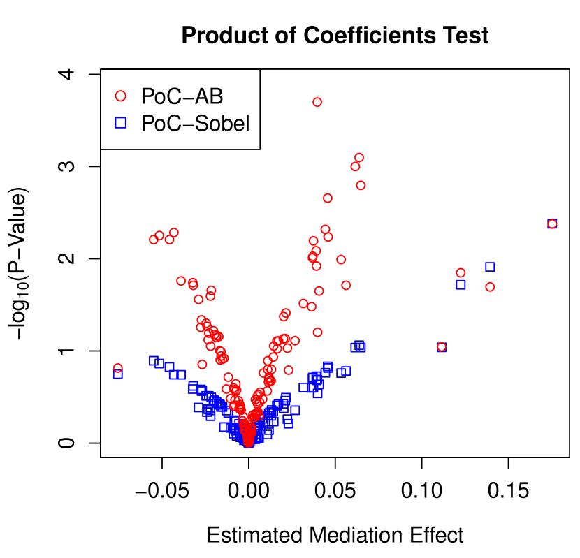
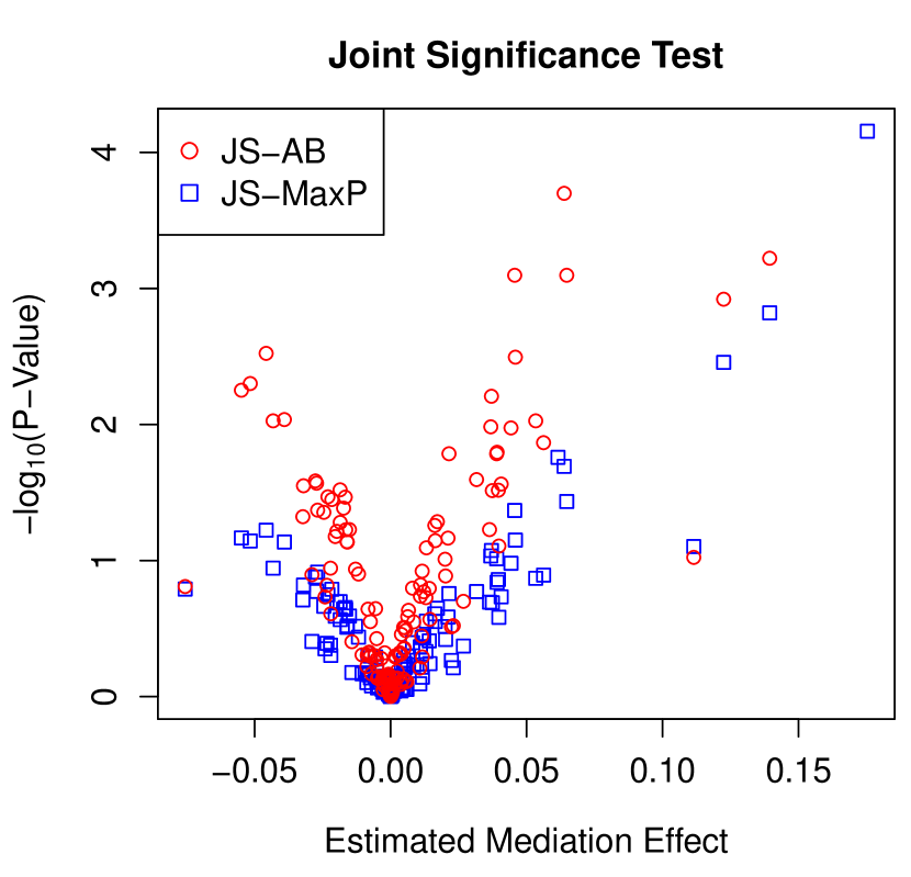
Figure 27: Volcano plots: $-\log_{10}(p\text{-values})$ versus their estimated mediation effects.

G.4 Confirmatory Analysis of Data via Double Bootstrap

We conduct a confirmatory analysis below, which aims to provide additional evidence of testing results yielded by AB methods. The confirmatory procedure leverages the the double bootstrap (DB) strategy as outlined in Section F.1. Analyzing the $p$-values yielded by DB can offer us additional insights into the underlying model. Let $\mathcal{D}_{obs}$ denote an observed dataset. We apply the two data processing methods (i) and (ii) in Section F.1 and obtain two processed datasets, denoted as $\mathcal{D}_{\alpha}$ and $\mathcal{D}_{\beta}$, respectively.

Confirmatory Analysis Procedure

Step 1. Given an observed dataset $\mathcal{D}_{obs}$, obtain two processed datasets $\mathcal{D}_{{\alpha}}$ and $\mathcal{D}_{{\beta}}$.
Step 2. Apply DB to $\mathcal{D}_{{obs}}$, i.e., for $b=1,\ldots,B$,

• apply ordinary bootstrap to $\mathcal{D}_{{obs}}$, and let $\mathcal{D}_{{obs},b}^{*}$ denote the bootstrapped data;

• apply AB with $\lambda=0$ to $\mathcal{D}_{obs,b}^{*}$ to obtain an estimated $p$-value $p_{obs,b}^{*}$.

Let $\mathcal{P}^{*}_{obs}=\{p_{obs,b}^{*}:b=1,\ldots,B\}$ be the set of estimated $p$-values.
Step 3. Apply DB to $\mathcal{D}_{\alpha}$ similarly to Step 2 above and obtain $\mathcal{P}^{*}_{\alpha}=\{p_{\alpha,b}^{*}:b=1,\ldots,B\}$.
Step 4. Apply DB to $\mathcal{D}_{\beta}$ similarly to Step 2 above and obtain $\mathcal{P}^{*}_{\beta}=\{p_{\beta,b}^{*}:b=1,\ldots,B\}$.

Interpretation of Results

We would observe different properties of $\mathcal{P}^{*}_{obs}$, $\mathcal{P}^{*}_{\alpha}$ and $\mathcal{P}^{*}_{\beta}$ under different scenarios of the true parameters. Specifically,

• when $\alpha_{S}=\beta_{M}=0$, QQ-plots of $\mathcal{P}^{*}_{obs}$, $\mathcal{P}^{*}_{\alpha}$ and $\mathcal{P}^{*}_{\beta}$ are all conservative;

• when $\alpha_{S}\neq 0$ and $\beta_{M}=0$, QQ-plots of $\mathcal{P}^{*}_{obs}$ and $\mathcal{P}^{*}_{\beta}$ would be close to diagonal, whereas QQ-plot of $\mathcal{P}^{*}_{\alpha}$ would be conservative;

• when $\alpha_{S}=0$ and $\beta_{M}\neq 0$, QQ-plots of $\mathcal{P}^{*}_{obs}$ and $\mathcal{P}^{*}_{\alpha}$ would be close to diagonal, whereas QQ-plot of $\mathcal{P}^{*}_{\beta}$ would be conservative.

• when $\alpha_{S}\neq 0$ and $\beta_{M}\neq 0$, QQ-plot of $\mathcal{P}^{*}_{obs}$ would bend upward, and QQ-plots of both $\mathcal{P}^{*}_{\alpha}$ are $\mathcal{P}^{*}_{\beta}$ close to the diagonal.

In another word, the observed patterns of $\mathcal{P}^{*}_{obs}$, $\mathcal{P}^{*}_{\alpha}$ and $\mathcal{P}^{*}_{\beta}$ can provide us additional credibility about the underlying true parameters.

We next apply the above DB procedure to our analyzed data. As previously reported in Section 6 of the main text, the mediator LAURIC.ACID (L.A) was selected by the AB test. As a comparison, we randomly pick another mediator, FA.12.0-OH (F.12), from the data that was not selected by the AB test. To affirm the testing results, we carry out the procedure above to obtain estimated $p$-values of testing the mediation effects via L.A and F.12 separately, presented in Figures 28 and 29 below. In particular,

• For the selected mediator L.A, Figure 28 exhibits patterns that are expected when data are generated from $\alpha_{S}\neq 0$ and $\beta_{M}\neq 0$, i.e. alternative hypotheses.

• For the non-selected mediator F.12, Figure 28 exhibits patterns that are expected when data are generated from $\alpha_{S}=0$ and $\beta_{M}\neq 0$, i.e. a null hypothesis.

Similar patterns have been observed across all the mediators. In short, our confirmatory analysis of the data substantiates that the chosen mediators indeed align with alternative hypotheses, reinforcing the credibility of our analysis results. The codes for reproducing the confirmatory analysis analysis are provided on our GitHub repository https://github.com/yinqiuhe/ABtest. Given the inherent complexity of real-world data, we recommend that practitioners exercise caution and make decisions in conjunction with domain-specific knowledge when interpreting results. Nevertheless, the confirmatory analysis via the double bootstrap paradigm provides a powerful tool that enables us to gather additional evidence ensuring our discoveries.

Figure 28: QQ-plots of $p$-values by DB for L.A (a selected mediator) with 95% confidence bands.

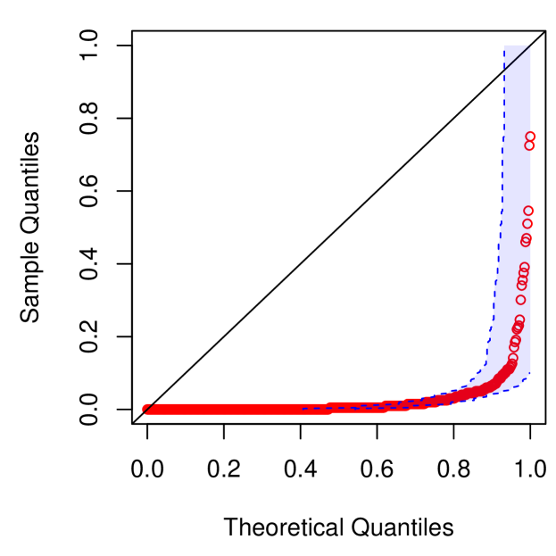
(a) $\mathcal{P}_{obs}^{*}$

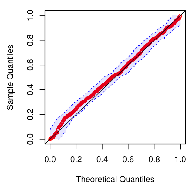
(b) $\mathcal{P}_{\alpha}^{*}$

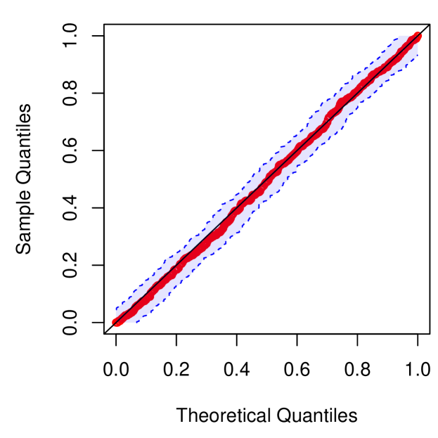
(c) $\mathcal{P}_{\beta}^{*}$

Figure 29: QQ-plots of $p$-values by DB for F.12 (a non-selected mediator) with 95% confidence bands.

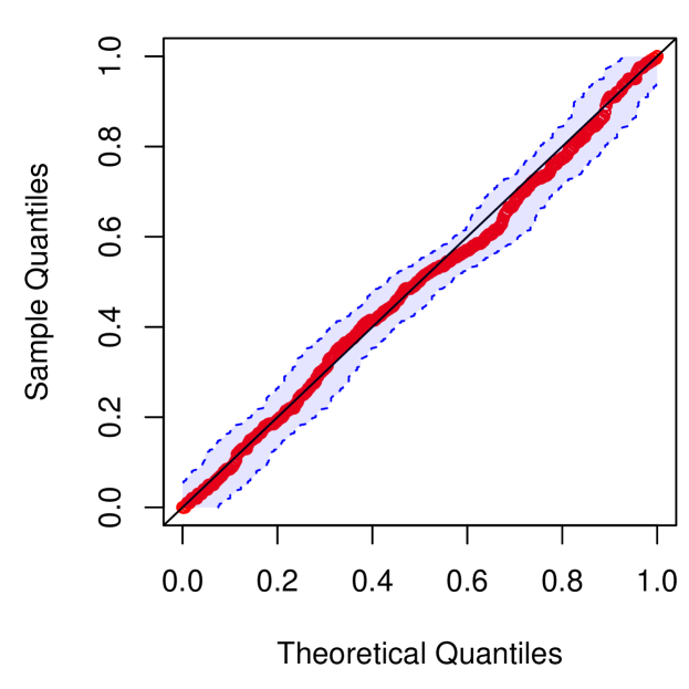
(a) $\mathcal{P}_{obs}^{*}$

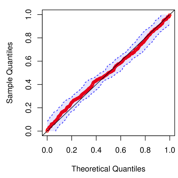
(b) $\mathcal{P}_{\alpha}^{*}$

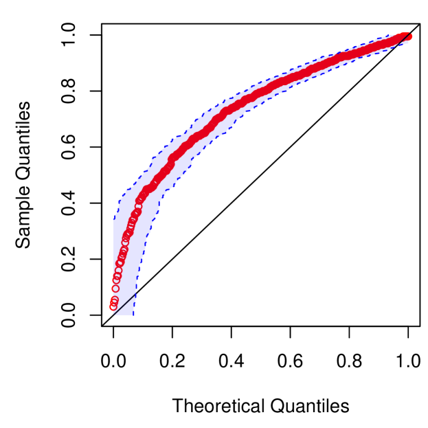
(c) $\mathcal{P}_{\beta}^{*}$

Appendix H Conservatism under Partially Linear Model

Similar conservatism issue of testing no-mediation effect has been observed in certain partially linear model. In particular, Hines et al. (2021) studied the identification and estimation of natural indirect effect under the following partially linear model

$$\mathrm{E}(M\mid S,\boldsymbol{X})= ~{}\alpha_{S}S+f(\boldsymbol{X}),$$ (63)

$$\mathrm{E}(Y\mid S,M,\boldsymbol{X})= ~{}\beta_{M}M+g(S,\boldsymbol{X}),$$ (64)

where $g(s,\boldsymbol{x})$ and $f(\boldsymbol{x})$ are arbitrary functions. Under the model (63)–(64) and standard identifiability assumptions (see details in Section 2 of Hines et al. (2021)), Hines et al. (2021) showed that $\mathrm{NIE}_{s\mid s^{*}}(s,\boldsymbol{x})=\mathrm{E}\left\{Y(s,M(s))-Y\left(s,M\left(s^{*}\right)\right)\mid\boldsymbol{X}=\boldsymbol{x}\right\}=\alpha_{S}\beta_{M}(s-s^{*})$. Hines et al. (2021) proposed a G-estimator, i.e., obtains estimators of coefficients $(\hat{\alpha}_{S},\hat{\beta}_{M})$ based on G-moment conditions. Hines et al. (2021) showed that $\hat{\alpha}_{S}\hat{\beta}_{M}$ is a consistent and asymptotic normal estimator for $\alpha_{S}\beta_{M}$ when (63)–(64) hold and either

1. the model for $f(\boldsymbol{X})$ is correctly specified;

2. $g(S,\boldsymbol{X})=\tau_{S}S+g(\boldsymbol{X})$ and the models for $g(\boldsymbol{X})$ and $\mathrm{E}(S\mid\boldsymbol{X})$ are both correctly specified.

Numerical studies in Figure 4 of Hines et al. (2021) showed that when testing no-mediation hypothesis, all the testing methods are conservative, which is similar to the observations under linear models.

When there exists exposure-mediator interaction in the outcome model, Section 8 of Hines et al. (2021) briefly discussed the following mean outcome model:

$$\mathrm{E}(Y\mid S,M,\boldsymbol{X})=\beta_{M}M+\theta SM+\tau_{S}S+g(\boldsymbol{X}).$$ (65)

Under (63) and (65) and standard identification assumptions, it is shown that

$$\mathrm{NIE}_{s\mid s^{*}}(s,\boldsymbol{x})=\Psi(s)(s-s^{*}),\quad\text{where}\quad\Psi(s)=\alpha_{S}(\beta_{M}+\theta s),$$ (66)

which is the same as that under the classical additive linear model with interaction term; see, e.g., Eq. (15) in Imai et al. (2010b). Given a specific value of $s$, we conjecture that classical tests would be conservative in the case of both $\alpha_{S}=0$ and $\beta_{M}+\theta s=0$. To illustrate this conservatism empirically, we conducted a simulation experiment under the model (63) and (66) with $f=g=0$. We use the R package mediation with nonparametric bootstrap to test no mediation effect $\Psi(s)=0$ at $s=0$ and $s=1$ separately. Results in Figure 30 aligns with our conjecture and shows clearly that the values of $(\alpha_{S},\beta_{M})$ leading to conservative performances vary with respect to $s$. We anticipate that the adaptive bootstrap test could be extended while considering a certain value of $s$. When the model functions are misspecified, the package of Hines et al. (2021) cannot be applied directly. It would be an interesting future direction to develop AB-type estimation and inference tools under the partially linear model with exposure-mediator interactions.

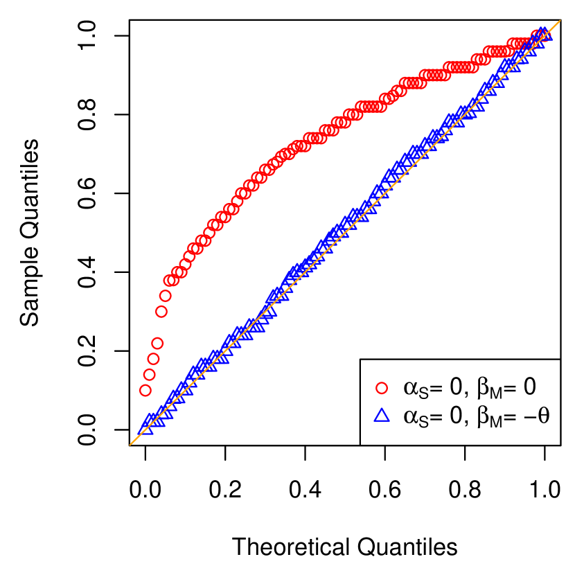
(a) Test $H_{0}:\Psi(0)=0$.

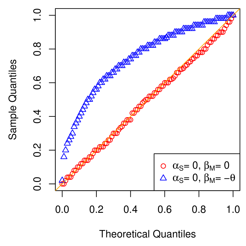
(b) Test $H_{0}:\Psi(1)=0$.

Figure 30: QQ-plots of p-values under the model with exposure-mediator interaction and $\theta=1$.

References

- Andrews (2001) Andrews, D. W. (2001) Testing when a parameter is on the boundary of the maintained hypothesis. Econometrica, 69, 683–734.
- Barfield et al. (2017) Barfield, R., Shen, J., Just, A. C., Vokonas, P. S., Schwartz, J., Baccarelli, A. A., VanderWeele, T. J. and Lin, X. (2017) Testing for the indirect effect under the null for genome-wide mediation analyses. Genetic Epidemiology, 41, 824–833.
- Baron and Kenny (1986) Baron, R. M. and Kenny, D. A. (1986) The moderator–mediator variable distinction in social psychological research: Conceptual, strategic, and statistical considerations. Journal of Personality and Social Psychology, 51, 1173–1182.
- Benjamini and Hochberg (1995) Benjamini, Y. and Hochberg, Y. (1995) Controlling the false discovery rate: a practical and powerful approach to multiple testing. Journal of the Royal Statistical Society: Series B (Methodological), 57, 289–300.
- Bickel and Freedman (1981) Bickel, P. J. and Freedman, D. A. (1981) Some asymptotic theory for the bootstrap. The annals of statistics, 9, 1196–1217.
- Bind et al. (2016) Bind, M.-A., Vanderweele, T., Coull, B. and Schwartz, J. (2016) Causal mediation analysis for longitudinal data with exogenous exposure. Biostatistics, 17, 122–134.
- Blum et al. (2020) Blum, M. G., Valeri, L., François, O., Cadiou, S., Siroux, V., Lepeule, J. and Slama, R. (2020) Challenges raised by mediation analysis in a high-dimension setting. Environmental Health Perspectives, 128, 055001.
- Bogomolov and Heller (2018) Bogomolov, M. and Heller, R. (2018) Assessing replicability of findings across two studies of multiple features. Biometrika, 105, 505–516.
- Chen (2016) Chen, S. X. (2016) Peter Hall’s contributions to the bootstrap. The Annals of Statistics, 44, 1821–1836.
- Dai et al. (2020) Dai, J. Y., Stanford, J. L. and LeBlanc, M. (2020) A multiple-testing procedure for high-dimensional mediation hypotheses. Journal of the American Statistical Association, 1–16.
- Daniel et al. (2015) Daniel, R., De Stavola, B., Cousens, S. and Vansteelandt, S. (2015) Causal mediation analysis with multiple mediators. Biometrics, 71, 1–14.
- Dayrit (2015) Dayrit, F. M. (2015) The properties of lauric acid and their significance in coconut oil. Journal of the American Oil Chemists’ Society, 92, 1–15.
- Derkach et al. (2020) Derkach, A., Moore, S. C., Boca, S. M. and Sampson, J. N. (2020) Group testing in mediation analysis. Statistics in Medicine, 39, 2423–2436.
- Djordjilović et al. (2020) Djordjilović, V., Hemerik, J. and Thoresen, M. (2020) On optimal two-stage testing of multiple mediators. arXiv preprint arXiv:2007.02844.
- Djordjilović et al. (2019) Djordjilović, V., Page, C. M., Gran, J. M., Nøst, T. H., Sandanger, T. M., Veierød, M. B. and Thoresen, M. (2019) Global test for high-dimensional mediation: Testing groups of potential mediators. Statistics in Medicine, 38, 3346–3360.
- Drton and Xiao (2016) Drton, M. and Xiao, H. (2016) Wald tests of singular hypotheses. Bernoulli, 22, 38–59.
- Du et al. (2022) Du, J., Zhou, X., Hao, W., Liu, Y., Jennifer, S. and Mukherjee, B. (2022) Methods for large-scale single mediator hypothesis testing: Possible choices and comparisons. arXiv preprint arXiv:2203.13293.
- Dufour et al. (2013) Dufour, J.-M., Renault, E. and Zinde-Walsh, V. (2013) Wald tests when restrictions are locally singular. arXiv preprint arXiv:1312.0569.
- Frisch and Waugh (1933) Frisch, R. and Waugh, F. V. (1933) Partial time regressions as compared with individual trends. Econometrica, 387–401.
- Fritz and MacKinnon (2007) Fritz, M. S. and MacKinnon, D. P. (2007) Required sample size to detect the mediated effect. Psychological Science, 18, 233–239.
- Fulcher et al. (2019) Fulcher, I. R., Shi, X. and Tchetgen, E. J. T. (2019) Estimation of natural indirect effects robust to unmeasured confounding and mediator measurement error. Epidemiology, 30, 825–834.
- Glonek (1993) Glonek, G. (1993) On the behaviour of wald statistics for the disjunction of two regular hypotheses. Journal of the Royal Statistical Society: Series B (Methodological), 55, 749–755.
- Guo et al. (2022) Guo, X., Li, R., Liu, J. and Zeng, M. (2022) High-dimensional mediation analysis for selecting DNA methylation loci mediating childhood trauma and cortisol stress reactivity. Journal of the American Statistical Association, 1–32.
- Hao and Song (2022) Hao, W. and Song, P. X.-K. (2022) A simultaneous likelihood test for joint mediation effects of multiple mediators. Statistica Sinica.
- Hayes (2017) Hayes, A. F. (2017) Introduction to mediation, moderation, and conditional process analysis: A regression-based approach. Guilford publications.
- He et al. (2023) He, Y., Song, P. X.-K. and Xu, G. (2023) ABtest. https://github.com/yinqiuhe/ABtest.
- Hines et al. (2021) Hines, O., Vansteelandt, S. and Diaz-Ordaz, K. (2021) Robust inference for mediated effects in partially linear models. Psychometrika, 1–24.
- Huang (2018) Huang, Y.-T. (2018) Joint significance tests for mediation effects of socioeconomic adversity on adiposity via epigenetics. The Annals of Applied Statistics, 12, 1535–1557.
- Huang (2019a) — (2019a) Genome-wide analyses of sparse mediation effects under composite null hypotheses. The Annals of Applied Statistics, 13, 60–84.
- Huang (2019b) — (2019b) Variance component tests of multivariate mediation effects under composite null hypotheses. Biometrics, 75, 1191–1204.
- Huang and Cai (2016) Huang, Y.-T. and Cai, T. (2016) Mediation analysis for survival data using semiparametric probit models. Biometrics, 72, 563–574.
- Huang and Pan (2016) Huang, Y.-T. and Pan, W.-C. (2016) Hypothesis test of mediation effect in causal mediation model with high-dimensional continuous mediators. Biometrics, 72, 402–413.
- Imai et al. (2010a) Imai, K., Keele, L. and Tingley, D. (2010a) A general approach to causal mediation analysis. Psychological Methods, 15, 309–334.
- Imai et al. (2010b) Imai, K., Keele, L. and Yamamoto, T. (2010b) Identification, inference and sensitivity analysis for causal mediation effects. Statistical Science, 25, 51–71.
- Imai and Yamamoto (2013) Imai, K. and Yamamoto, T. (2013) Identification and sensitivity analysis for multiple causal mechanisms: Revisiting evidence from framing experiments. Political Analysis, 21, 141–171.
- Imbens and Rubin (2015) Imbens, G. W. and Rubin, D. B. (2015) Causal inference in statistics, social, and biomedical sciences. Cambridge University Press.
- Jérolon et al. (2020) Jérolon, A., Baglietto, L., Birmelé, E., Alarcon, F. and Perduca, V. (2020) Causal mediation analysis in presence of multiple mediators uncausally related. The International Journal of Biostatistics, 17, 191–221.
- Judd and Kenny (1981) Judd, C. M. and Kenny, D. A. (1981) Estimating the effects of social intervention. Cambridge University Press.
- Laber and Murphy (2011) Laber, E. B. and Murphy, S. A. (2011) Adaptive confidence intervals for the test error in classification. Journal of the American Statistical Association, 106, 904–913.
- Liu et al. (2021) Liu, Z., Shen, J., Barfield, R., Schwartz, J., Baccarelli, A. A. and Lin, X. (2021) Large-scale hypothesis testing for causal mediation effects with applications in genome-wide epigenetic studies. Journal of the American Statistical Association, 1–15.
- Loh et al. (2021) Loh, W. W., Moerkerke, B., Loeys, T. and Vansteelandt, S. (2021) Disentangling indirect effects through multiple mediators without assuming any causal structure among the mediators. Psychological Methods.
- MacKinnon (2008) MacKinnon, D. (2008) Introduction to Statistical Mediation Analysis. Multivariate Applications Book Series. Taylor & Francis.
- MacKinnon and Fairchild (2009) MacKinnon, D. P. and Fairchild, A. J. (2009) Current directions in mediation analysis. Current Directions in Psychological Science, 18, 16–20.
- MacKinnon et al. (2002) MacKinnon, D. P., Lockwood, C. M., Hoffman, J. M., West, S. G. and Sheets, V. (2002) A comparison of methods to test mediation and other intervening variable effects. Psychological Methods, 7, 83–104.
- MacKinnon et al. (2004) MacKinnon, D. P., Lockwood, C. M. and Williams, J. (2004) Confidence limits for the indirect effect: Distribution of the product and resampling methods. Multivariate Behavioral Research, 39, 99–128.
- McKeague and Qian (2015) McKeague, I. W. and Qian, M. (2015) An adaptive resampling test for detecting the presence of significant predictors. Journal of the American Statistical Association, 110, 1422–1433.
- McKeague and Qian (2019) — (2019) Marginal screening of 22 tables in large-scale case-control studies. Biometrics, 75, 163–171.
- Miles and Chambaz (2021) Miles, C. H. and Chambaz, A. (2021) Optimal tests of the composite null hypothesis arising in mediation analysis. arXiv preprint arXiv:2107.07575.
- Pearl (2001) Pearl, J. (2001) Direct and indirect effects. In Proceedings of the Seventeenth Conference on Uncertainty in Artificial Intelligence, UAI’01, 411–420. San Francisco, CA, USA: Morgan Kaufmann Publishers Inc.
- Perng et al. (2019) Perng, W. et al. (2019) The early life exposure in mexico to environmental toxicants (ELEMENT) project. British Medical Journal Open, 9, e030427.
- Robins and Greenland (1992) Robins, J. M. and Greenland, S. (1992) Identifiability and exchangeability for direct and indirect effects. Epidemiology, 3, 143–155.
- Rubin (1980) Rubin, D. B. (1980) Randomization analysis of experimental data: The fisher randomization test comment. Journal of the American statistical association, 75, 591–593.
- Sampson et al. (2018) Sampson, J. N., Boca, S. M., Moore, S. C. and Heller, R. (2018) FWER and FDR control when testing multiple mediators. Bioinformatics, 34, 2418–2424.
- Shi and Li (2022) Shi, C. and Li, L. (2022) Testing mediation effects using logic of boolean matrices. Journal of the American Statistical Association, 117, 2014–2027.
- Sobel (1982) Sobel, M. E. (1982) Asymptotic confidence intervals for indirect effects in structural equation models. Sociological Methodology, 13, 290–312.
- Sohn and Li (2019) Sohn, M. B. and Li, H. (2019) Compositional mediation analysis for microbiome studies. The Annals of Applied Statistics, 13, 661–681.
- Tingley et al. (2014) Tingley, D., Yamamoto, T., Hirose, K., Keele, L. and Imai, K. (2014) Mediation: R package for causal mediation analysis. Journal of Statistical Software, 59, 1–38.
- van der Vaart (2000) van der Vaart, A. W. (2000) Asymptotic statistics, vol. 3 of Cambridge Series in Statistical and Probabilistic Mathematics. Cambridge University Press.
- Valeri and VanderWeele (2013) Valeri, L. and VanderWeele, T. J. (2013) Mediation analysis allowing for exposure–mediator interactions and causal interpretation: theoretical assumptions and implementation with SAS and SPSS macros. Psychological Methods, 18, 137–155.
- Van Garderen and Van Giersbergen (2022) Van Garderen, K. and Van Giersbergen, N. (2022) A nearly similar powerful test for mediation. Tech. rep.
- VanderWeele (2011) VanderWeele, T. J. (2011) Causal mediation analysis with survival data. Epidemiology, 22, 582–585.
- VanderWeele (2015) — (2015) Explanation in causal inference: methods for mediation and interaction. Oxford University Press.
- VanderWeele and Vansteelandt (2009) VanderWeele, T. J. and Vansteelandt, S. (2009) Conceptual issues concerning mediation, interventions and composition. Statistics and its Interface, 2, 457–468.
- VanderWeele and Vansteelandt (2010) — (2010) Odds ratios for mediation analysis for a dichotomous outcome. American Journal of Epidemiology, 172, 1339–1348.
- VanderWeele and Vansteelandt (2014) — (2014) Mediation analysis with multiple mediators. Epidemiologic Methods, 2, 95–115.
- VanderWeele et al. (2014) VanderWeele, T. J., Vansteelandt, S. and Robins, J. M. (2014) Effect decomposition in the presence of an exposure-induced mediator-outcome confounder. Epidemiology (Cambridge, Mass.), 25, 300.
- Vansteelandt and Daniel (2017) Vansteelandt, S. and Daniel, R. M. (2017) Interventional effects for mediation analysis with multiple mediators. Epidemiology (Cambridge, Mass.), 28, 258.
- Wang et al. (2018) Wang, H. J., McKeague, I. W. and Qian, M. (2018) Testing for marginal linear effects in quantile regression. Journal of the Royal Statistical Society: Series B (Statistical Methodology), 80, 433–452.
- Zhao et al. (2014) Zhao, S. D., Cai, T. T. and Li, H. (2014) More powerful genetic association testing via a new statistical framework for integrative genomics. Biometrics, 70, 881–890.
- Zhou et al. (2020) Zhou, R. R., Wang, L. and Zhao, S. D. (2020) Estimation and inference for the indirect effect in high-dimensional linear mediation models. Biometrika, 107, 573–589.

References

- Andrews (2001) Andrews, D. W. (2001) Testing when a parameter is on the boundary of the maintained hypothesis. Econometrica, 69, 683–734.
- Barfield et al. (2017) Barfield, R., Shen, J., Just, A. C., Vokonas, P. S., Schwartz, J., Baccarelli, A. A., VanderWeele, T. J. and Lin, X. (2017) Testing for the indirect effect under the null for genome-wide mediation analyses. Genetic Epidemiology, 41, 824–833.
- Baron and Kenny (1986) Baron, R. M. and Kenny, D. A. (1986) The moderator–mediator variable distinction in social psychological research: Conceptual, strategic, and statistical considerations. Journal of Personality and Social Psychology, 51, 1173–1182.
- Benjamini and Hochberg (1995) Benjamini, Y. and Hochberg, Y. (1995) Controlling the false discovery rate: a practical and powerful approach to multiple testing. Journal of the Royal Statistical Society: Series B (Methodological), 57, 289–300.
- Bickel and Freedman (1981) Bickel, P. J. and Freedman, D. A. (1981) Some asymptotic theory for the bootstrap. The annals of statistics, 9, 1196–1217.
- Bind et al. (2016) Bind, M.-A., Vanderweele, T., Coull, B. and Schwartz, J. (2016) Causal mediation analysis for longitudinal data with exogenous exposure. Biostatistics, 17, 122–134.
- Blum et al. (2020) Blum, M. G., Valeri, L., François, O., Cadiou, S., Siroux, V., Lepeule, J. and Slama, R. (2020) Challenges raised by mediation analysis in a high-dimension setting. Environmental Health Perspectives, 128, 055001.
- Bogomolov and Heller (2018) Bogomolov, M. and Heller, R. (2018) Assessing replicability of findings across two studies of multiple features. Biometrika, 105, 505–516.
- Chen (2016) Chen, S. X. (2016) Peter Hall’s contributions to the bootstrap. The Annals of Statistics, 44, 1821–1836.
- Dai et al. (2020) Dai, J. Y., Stanford, J. L. and LeBlanc, M. (2020) A multiple-testing procedure for high-dimensional mediation hypotheses. Journal of the American Statistical Association, 1–16.
- Daniel et al. (2015) Daniel, R., De Stavola, B., Cousens, S. and Vansteelandt, S. (2015) Causal mediation analysis with multiple mediators. Biometrics, 71, 1–14.
- Dayrit (2015) Dayrit, F. M. (2015) The properties of lauric acid and their significance in coconut oil. Journal of the American Oil Chemists’ Society, 92, 1–15.
- Derkach et al. (2020) Derkach, A., Moore, S. C., Boca, S. M. and Sampson, J. N. (2020) Group testing in mediation analysis. Statistics in Medicine, 39, 2423–2436.
- Djordjilović et al. (2020) Djordjilović, V., Hemerik, J. and Thoresen, M. (2020) On optimal two-stage testing of multiple mediators. arXiv preprint arXiv:2007.02844.
- Djordjilović et al. (2019) Djordjilović, V., Page, C. M., Gran, J. M., Nøst, T. H., Sandanger, T. M., Veierød, M. B. and Thoresen, M. (2019) Global test for high-dimensional mediation: Testing groups of potential mediators. Statistics in Medicine, 38, 3346–3360.
- Drton and Xiao (2016) Drton, M. and Xiao, H. (2016) Wald tests of singular hypotheses. Bernoulli, 22, 38–59.
- Du et al. (2022) Du, J., Zhou, X., Hao, W., Liu, Y., Jennifer, S. and Mukherjee, B. (2022) Methods for large-scale single mediator hypothesis testing: Possible choices and comparisons. arXiv preprint arXiv:2203.13293.
- Dufour et al. (2013) Dufour, J.-M., Renault, E. and Zinde-Walsh, V. (2013) Wald tests when restrictions are locally singular. arXiv preprint arXiv:1312.0569.
- Frisch and Waugh (1933) Frisch, R. and Waugh, F. V. (1933) Partial time regressions as compared with individual trends. Econometrica, 387–401.
- Fritz and MacKinnon (2007) Fritz, M. S. and MacKinnon, D. P. (2007) Required sample size to detect the mediated effect. Psychological Science, 18, 233–239.
- Fulcher et al. (2019) Fulcher, I. R., Shi, X. and Tchetgen, E. J. T. (2019) Estimation of natural indirect effects robust to unmeasured confounding and mediator measurement error. Epidemiology, 30, 825–834.
- Glonek (1993) Glonek, G. (1993) On the behaviour of wald statistics for the disjunction of two regular hypotheses. Journal of the Royal Statistical Society: Series B (Methodological), 55, 749–755.
- Guo et al. (2022) Guo, X., Li, R., Liu, J. and Zeng, M. (2022) High-dimensional mediation analysis for selecting DNA methylation loci mediating childhood trauma and cortisol stress reactivity. Journal of the American Statistical Association, 1–32.
- Hao and Song (2022) Hao, W. and Song, P. X.-K. (2022) A simultaneous likelihood test for joint mediation effects of multiple mediators. Statistica Sinica.
- Hayes (2017) Hayes, A. F. (2017) Introduction to mediation, moderation, and conditional process analysis: A regression-based approach. Guilford publications.
- He et al. (2023) He, Y., Song, P. X.-K. and Xu, G. (2023) ABtest. https://github.com/yinqiuhe/ABtest.
- Hines et al. (2021) Hines, O., Vansteelandt, S. and Diaz-Ordaz, K. (2021) Robust inference for mediated effects in partially linear models. Psychometrika, 1–24.
- Huang (2018) Huang, Y.-T. (2018) Joint significance tests for mediation effects of socioeconomic adversity on adiposity via epigenetics. The Annals of Applied Statistics, 12, 1535–1557.
- Huang (2019a) — (2019a) Genome-wide analyses of sparse mediation effects under composite null hypotheses. The Annals of Applied Statistics, 13, 60–84.
- Huang (2019b) — (2019b) Variance component tests of multivariate mediation effects under composite null hypotheses. Biometrics, 75, 1191–1204.
- Huang and Cai (2016) Huang, Y.-T. and Cai, T. (2016) Mediation analysis for survival data using semiparametric probit models. Biometrics, 72, 563–574.
- Huang and Pan (2016) Huang, Y.-T. and Pan, W.-C. (2016) Hypothesis test of mediation effect in causal mediation model with high-dimensional continuous mediators. Biometrics, 72, 402–413.
- Imai et al. (2010a) Imai, K., Keele, L. and Tingley, D. (2010a) A general approach to causal mediation analysis. Psychological Methods, 15, 309–334.
- Imai et al. (2010b) Imai, K., Keele, L. and Yamamoto, T. (2010b) Identification, inference and sensitivity analysis for causal mediation effects. Statistical Science, 25, 51–71.
- Imai and Yamamoto (2013) Imai, K. and Yamamoto, T. (2013) Identification and sensitivity analysis for multiple causal mechanisms: Revisiting evidence from framing experiments. Political Analysis, 21, 141–171.
- Imbens and Rubin (2015) Imbens, G. W. and Rubin, D. B. (2015) Causal inference in statistics, social, and biomedical sciences. Cambridge University Press.
- Jérolon et al. (2020) Jérolon, A., Baglietto, L., Birmelé, E., Alarcon, F. and Perduca, V. (2020) Causal mediation analysis in presence of multiple mediators uncausally related. The International Journal of Biostatistics, 17, 191–221.
- Judd and Kenny (1981) Judd, C. M. and Kenny, D. A. (1981) Estimating the effects of social intervention. Cambridge University Press.
- Laber and Murphy (2011) Laber, E. B. and Murphy, S. A. (2011) Adaptive confidence intervals for the test error in classification. Journal of the American Statistical Association, 106, 904–913.
- Liu et al. (2021) Liu, Z., Shen, J., Barfield, R., Schwartz, J., Baccarelli, A. A. and Lin, X. (2021) Large-scale hypothesis testing for causal mediation effects with applications in genome-wide epigenetic studies. Journal of the American Statistical Association, 1–15.
- Loh et al. (2021) Loh, W. W., Moerkerke, B., Loeys, T. and Vansteelandt, S. (2021) Disentangling indirect effects through multiple mediators without assuming any causal structure among the mediators. Psychological Methods.
- MacKinnon (2008) MacKinnon, D. (2008) Introduction to Statistical Mediation Analysis. Multivariate Applications Book Series. Taylor & Francis.
- MacKinnon and Fairchild (2009) MacKinnon, D. P. and Fairchild, A. J. (2009) Current directions in mediation analysis. Current Directions in Psychological Science, 18, 16–20.
- MacKinnon et al. (2002) MacKinnon, D. P., Lockwood, C. M., Hoffman, J. M., West, S. G. and Sheets, V. (2002) A comparison of methods to test mediation and other intervening variable effects. Psychological Methods, 7, 83–104.
- MacKinnon et al. (2004) MacKinnon, D. P., Lockwood, C. M. and Williams, J. (2004) Confidence limits for the indirect effect: Distribution of the product and resampling methods. Multivariate Behavioral Research, 39, 99–128.
- McKeague and Qian (2015) McKeague, I. W. and Qian, M. (2015) An adaptive resampling test for detecting the presence of significant predictors. Journal of the American Statistical Association, 110, 1422–1433.
- McKeague and Qian (2019) — (2019) Marginal screening of 22 tables in large-scale case-control studies. Biometrics, 75, 163–171.
- Miles and Chambaz (2021) Miles, C. H. and Chambaz, A. (2021) Optimal tests of the composite null hypothesis arising in mediation analysis. arXiv preprint arXiv:2107.07575.
- Pearl (2001) Pearl, J. (2001) Direct and indirect effects. In Proceedings of the Seventeenth Conference on Uncertainty in Artificial Intelligence, UAI’01, 411–420. San Francisco, CA, USA: Morgan Kaufmann Publishers Inc.
- Perng et al. (2019) Perng, W. et al. (2019) The early life exposure in mexico to environmental toxicants (ELEMENT) project. British Medical Journal Open, 9, e030427.
- Robins and Greenland (1992) Robins, J. M. and Greenland, S. (1992) Identifiability and exchangeability for direct and indirect effects. Epidemiology, 3, 143–155.
- Rubin (1980) Rubin, D. B. (1980) Randomization analysis of experimental data: The fisher randomization test comment. Journal of the American statistical association, 75, 591–593.
- Sampson et al. (2018) Sampson, J. N., Boca, S. M., Moore, S. C. and Heller, R. (2018) FWER and FDR control when testing multiple mediators. Bioinformatics, 34, 2418–2424.
- Shi and Li (2022) Shi, C. and Li, L. (2022) Testing mediation effects using logic of boolean matrices. Journal of the American Statistical Association, 117, 2014–2027.
- Sobel (1982) Sobel, M. E. (1982) Asymptotic confidence intervals for indirect effects in structural equation models. Sociological Methodology, 13, 290–312.
- Sohn and Li (2019) Sohn, M. B. and Li, H. (2019) Compositional mediation analysis for microbiome studies. The Annals of Applied Statistics, 13, 661–681.
- Tingley et al. (2014) Tingley, D., Yamamoto, T., Hirose, K., Keele, L. and Imai, K. (2014) Mediation: R package for causal mediation analysis. Journal of Statistical Software, 59, 1–38.
- van der Vaart (2000) van der Vaart, A. W. (2000) Asymptotic statistics, vol. 3 of Cambridge Series in Statistical and Probabilistic Mathematics. Cambridge University Press.
- Valeri and VanderWeele (2013) Valeri, L. and VanderWeele, T. J. (2013) Mediation analysis allowing for exposure–mediator interactions and causal interpretation: theoretical assumptions and implementation with SAS and SPSS macros. Psychological Methods, 18, 137–155.
- Van Garderen and Van Giersbergen (2022) Van Garderen, K. and Van Giersbergen, N. (2022) A nearly similar powerful test for mediation. Tech. rep.
- VanderWeele (2011) VanderWeele, T. J. (2011) Causal mediation analysis with survival data. Epidemiology, 22, 582–585.
- VanderWeele (2015) — (2015) Explanation in causal inference: methods for mediation and interaction. Oxford University Press.
- VanderWeele and Vansteelandt (2009) VanderWeele, T. J. and Vansteelandt, S. (2009) Conceptual issues concerning mediation, interventions and composition. Statistics and its Interface, 2, 457–468.
- VanderWeele and Vansteelandt (2010) — (2010) Odds ratios for mediation analysis for a dichotomous outcome. American Journal of Epidemiology, 172, 1339–1348.
- VanderWeele and Vansteelandt (2014) — (2014) Mediation analysis with multiple mediators. Epidemiologic Methods, 2, 95–115.
- VanderWeele et al. (2014) VanderWeele, T. J., Vansteelandt, S. and Robins, J. M. (2014) Effect decomposition in the presence of an exposure-induced mediator-outcome confounder. Epidemiology (Cambridge, Mass.), 25, 300.
- Vansteelandt and Daniel (2017) Vansteelandt, S. and Daniel, R. M. (2017) Interventional effects for mediation analysis with multiple mediators. Epidemiology (Cambridge, Mass.), 28, 258.
- Wang et al. (2018) Wang, H. J., McKeague, I. W. and Qian, M. (2018) Testing for marginal linear effects in quantile regression. Journal of the Royal Statistical Society: Series B (Statistical Methodology), 80, 433–452.
- Zhao et al. (2014) Zhao, S. D., Cai, T. T. and Li, H. (2014) More powerful genetic association testing via a new statistical framework for integrative genomics. Biometrics, 70, 881–890.
- Zhou et al. (2020) Zhou, R. R., Wang, L. and Zhao, S. D. (2020) Estimation and inference for the indirect effect in high-dimensional linear mediation models. Biometrika, 107, 573–589.