Excited States in Warm and Hot Dense Matter

Abstract

Accurate modeling of warm and hot dense matter is challenging in part due to the multitude of excited states that must be considered. In thermal density functional theory, these excited states are averaged over to produce a single, averaged, thermal ground state. Here we present a variational framework and model that includes explicit excited states. In this framework an excited state is defined by a set of effective one-electron occupation factors and the corresponding energy is defined by the effective one-body energy with an exchange and correlation term. The variational framework is applied to an atom-in-plasma model (a generalization of the so-called average atom model). Comparisons with a density functional theory based average atom model generally reveal good agreement in the calculated pressure, but the new model also gives access to the excitation energies and charge state distributions.

I Introduction

In warm and hot dense matter the electronic structure comprises a complex and very large set of excited states of the Hamiltonian. Electrons are excited to populate these states through collisions and absorption of electrons and photons. The resulting properties of the plasma, such as the equation of state (EOS), opacity, and transport coefficients, can, in principle, be calculated by taking appropriate averages over these excited states. Experiments can probe in detail these excited states ciricosta2012direct ; nagayama19 ; bailey15 ; kritcher2020measurement ; fletcher15 ; hollebon19 ; vinko2020time , providing stringent tests of our models.

There are many approaches to modeling warm and hot dense matter. Broadly speaking, at lower densities, a particularly successful approach is to start with the atomic structure of the isolated atoms or ions, and then to correct for plasma effects hakel06 ; colgan16 ; iglesias1996updated ; Stewart66lowering . Typically, these models become less successful at higher densities where a consistent treatment of plasma effects becomes crucial. At high densities, notable methods include path-integral Monte-Carlo (PIMC) militzer15 ; pollock1984simulation and density functional theory (DFT) based simulations collins95 ; hu2011first ; holst2008thermophysical ; starrett20ms . PIMC is so far largely limited to EOS applications and lower $Z$ materials. The widely popular DFT hohenberg , through its finite temperature extension mermin65 , has been applied to a wide variety of properties and is generally very successful.

However, attempts to apply DFT to the opacity of moderately or non-degenerate systems reveals a fundamental weakness of the approach shaffer22dense ; karasiev2022first ; gill2021time . As shown in these references, the calculated opacities differ wildly from the measured data. In DFT, it is the properties of the (thermal) ground state of the system that are calculated. To calculate excited state properties, time-dependent (TD-) DFT zangwill80 ; runge84 or ensemble DFT (EDFT) theophilou1979energy ; gross1988rayleigh ; gross1988density ; oliveira1988density is required.

TD-DFT calculations performed using the adiabatic local density approximation (ALDA) ullrich2011time fail dramatically when applied to these opacity problems gill2021time ; ullrich2014time . Although TD-DFT in principle is exact and allows for the calculation of all excited state properties, the ALDA uses only the instantaneous density for evaluation of the exchange-correlation functional. Multiple excitations are known to arise from nonadiabatic electron correlation effects that are neglected in the ALDA. This indicates that to properly treat multiple excitations, memory and dissipation effects need to be included explicitly in the exchange-correlation functional maitra2004double ; ullrich2006time ; sangalli2011double ; elliott2011perspectives . Hence, despite being in principle exact, in practice for these problems, the standard approximations (e.g., ALDA) are grossly inadequate.

The EDFT approach is an alternative to TD-DFT for calculating excited states, and is perhaps more naturally suited for inclusion of multiple excitations. This approach, formulated via a variational principle for ensembles of excited states, provides a modified Hohenberg-Kohn theorem that establishes an exact mapping between the potential and ensemble density. The benefit of this approach is that, via a corresponding Kohn-Sham scheme, the density for an ensemble of multiple excited states can be solved for simultaneously, and the energies of the excited states can be obtained. While this approach has that particular advantage, it is less frequently used than TD-DFT and many open questions remain, such as how to construct exchange-correlation functionals that go beyond the “quasi-LDA” kohn1986density and how to address the issue of ghost states gidopoulos2002spurious , which are in some ways analogous to electron self-interaction in ground-state DFT. Furthermore, temperature effects are not addressed in this approach. The approach we take in this paper is more similar to EDFT than to TD-DFT, though it is not formulated on a rigorous theoretical foundation, but instead more closely follows atomic physics approaches for calculating excited states. However, unlike EDFT, temperature is included explicitly in our approach.

In DFT the energy is divided into that of a non-interacting system (that gives the same electron density as the full interacting system) and a correction (the exchange and correlation term). Currently, the most accurate numerical scheme uses the Kohn-Sham (KS) approach kohn1965self . In KS-DFT, the non-interacting energy is found by solving a single-particle Schrödinger equation for an effective one-body interaction potential, determined by minimising the energy with respect to the density. This solution gives the eigenstates of this effective Hamiltonian and the electronic density is constructed by filling these states according to Fermi-Dirac statistics. Even at elevated temperatures this scheme is used, resulting in a set of KS states that are fractionally occupied.

While these KS states are formally not physical states, with only the density being physical, their proximity to real, physical states is vital for accurate predictions from the model and is reflected in, for example, Hugoniot predictions ottoway2021effect ; kritcher2020measurement ; bethkenhagen2023properties . At elevated temperatures therefore, the KS scheme, in which all excited states are represented by a single, averaged excited state, is expected to be a poorer approximation than at zero temperature where, in reality, there is only one occupied state (the ground state) gonis2018extension . This (the single averaged excited state) is also the reason why, for non-degenerate plasmas, the DFT predictions of opacity fail so spectacularly in practice.

A clue to a path forward may be found in the isolated atom approach to opacity sampson09 ; fontes2015alamos . In that field, an approach known as configuration-average approximation is very similar in practice to the KS-DFT scheme. One constructs an effective one body interaction potential for the ion or atom, includes an exchange and correlation correction, and solves the equations self-consistently. The key difference is that one does not use Fermi-Dirac occupations. Rather, one picks the occupations of the eigenstates to resemble desired excited states. Instead of there being one, averaged excited state, there are many different excited states, each corresponding to a particular distinct set of chosen occupations. This approach provides reasonable opacities in non-degenerate plasmas nagayama19 ; sampson09 ; fontes2015alamos .

However, this isolated atom approach suffers from two major drawbacks when applied to the dense plasma regime: first, it generally ignores, or treats inconsistently, the free electrons; second, it is not variationally derived from an energy expression, and so is generally not reliable for EOS. A number of works have improved this situation gill2023superconfiguration ; bar1989super ; blenski07 ; piron13 ; pain17 , but a practical variational framework has remained elusive.

In this work we give a variationally derived model that contains multiple distinct excited states, and includes free electrons consistently. As in the isolated atom approach, the excited states are defined by a chosen set of occupations. The energy of each excited state is calculated from an effective one-particle system with exchange and correlation corrections. In the limit of one excited state with Fermi-Dirac occupations, this model recovers the KS-DFT. We give the derivation of this model and apply it to electronic structure and EOS calculations in the dense plasma regime. For the application considered (excited atoms in a plasma), the model can be viewed as an extension to the work of liberman ; liberman1982inferno , where the author used DFT to get the averaged properties of an atom in a plasma.

II Free Energy

We consider an ensemble of nuclei and electrons in a volume $V$ and at temperature $T$. In Hartree atomic units, the free energy of the system is

$$\begin{split}F=&\sum_{x}W_{x}[E_{x}-TS_{x}]+T\sum_{x}W_{x}\log W_{x}\end{split}$$ (1)

where the sum over $x$ is over non-degenerate (in energy) excited states. The energy $E_{x}$ is approximated by

$$E_{x}=E_{x}^{(0)}+E_{x}^{el}+E_{x}^{xc}$$ (2)

where the effective single particle kinetic energy is

$$E_{x}^{(0)}=\sum_{i\in x}n_{x,i}\int_{V}d^{3}r\psi_{x,i}^{*}(-\frac{1}{2}\nabla^{2})\psi_{x,i}$$ (3)

with $\psi_{x,i}({\bm{r}})$ the orbital and $n_{x,i}$ the occupation factor for the $i^{th}$ eigenstate of excited state $x$. $E_{x}^{el}$ is the electrostatic energy

$$\begin{split}E_{x}^{el}=&\frac{1}{2}\int_{V}d^{3}r\int d^{3}r^{\prime}\frac{n_{x}({\bm{r}})n_{x}({\bm{r}}^{\prime})}{|{\bm{r}}-{\bm{r}}^{\prime}|}\\ &+\frac{1}{2}\sum_{m}\sum_{n\in V,n\neq m}\frac{Z_{n}Z_{m}}{|{\bm{R}_{n}}-{\bm{R}_{m}}|}\\ &-\sum_{n\in V}Z_{n}\int d^{3}r\frac{n_{x}({\bm{r}})}{|{\bm{r}}-{\bm{R}_{n}}|}\\ \end{split}$$ (4)

with $\bm{R}_{i}$ the position vector of nucleus $i$, and $n_{x}({\bm{r}})$ the electron density of excited state $x$

$$n_{x}({\bm{r}})=\sum_{i\in x}n_{x,i}|\psi_{x,i}({\bm{r}})|^{2}$$ (5)

and $Z_{n}$ is the nuclear charge of nucleus $n$. $E_{x}^{xc}$ is the exchange and correlation energy, which we approximate with the local density approximation

$$E_{x}^{xc}=\int_{V}d^{3}r\,\epsilon^{xc}[n_{x}({\bm{r}})]$$ (6)

The entropy has been split into two contributions (see appendix); a term due to the entropy of the excited state $S_{x}$

$$\begin{split}S_{x}=&-\int_{V}d^{3}r\sum_{i\in x}|\psi_{x,i}(r)|^{2}\\ &\times\left[n_{x,i}\log n_{x,i}+(1-n_{x,i})\log(1-n_{x,i})\right]\\ \end{split}$$ (7)

and a term due to the entropy of mixing $\sum_{x}W_{x}\log W_{x}$, where $W_{x}$ is the probability of excited state $x$.

II.1 Constrained Free Energy

Before minimising this free energy, the following constraints are added

$$\sum_{i\in x}\lambda_{x,i}\left[\int_{V}d^{3}r|\psi_{x,i}|^{2}-1\right]=0$$ (8a)

$$B\sum_{x}W_{x}=1$$ (8b)

$$\gamma\sum_{x}W_{x}\big{[}\int_{V}d^{3}rn_{x}({\bm{r}})-Z_{x}\big{]}=0$$ (8c)

$$\sum_{x,i}\mu_{x,i}W_{x}\int_{V}d^{3}r|\psi_{x,i}(r)|^{2}[n_{x,i}-f_{x,i}]=0$$ (8d)

where $\lambda_{x,i}$, $B$, $\gamma$ and $\mu_{x,i}$ are Lagrange multipliers. Equation (8a) ensures normalization of the orbitals, equation (8b) ensures that the probabilities $W_{x}$ sum to 1, equation (8c) requires overall charge neutrality of the excited states, and equation (8d) fixes the occupation factors $n_{x,i}$ to be given by the chosen inputs $f_{x,i}$. This last requirement is how we define an given excited state $x$.

II.2 Minimization of the Free Energy

We require the following to be true

$$\frac{\delta\Omega}{\delta\psi_{x,i}^{*}({\bm{r}})}=0$$ (9a)

$$\frac{\partial\Omega}{\partial n_{x,i}}=0$$ (9b)

$$\frac{\partial\Omega}{\partial W_{x}}=0$$ (9c)

where $\Omega$ is the constrained free energy. Applying the first of these, we obtain

$$\begin{split}0=&W_{x}\left[n_{x,i}[-\frac{1}{2}\nabla^{2}+V_{x}^{el}(r)+V_{x}^{xc}(r)]-\lambda_{x,i}\right]\psi_{x,i}(r)\\ &+W_{x}T\left[n_{x,i}\log n_{x,i}+(1-n_{x,i})\log(1-n_{x,i})\right]\psi_{x,i}(r)\\ &-W_{x}\gamma n_{x,i}\psi_{x,i}(r)-W_{x}\mu_{x,i}n_{x,i}\psi_{x,i}(r)\end{split}$$ (10)

which can be rewritten as

$$\begin{split}\left[-\frac{1}{2}\nabla^{2}+V_{x}^{el}({\bm{r}})+V_{x}^{xc}({\bm{r}})-\gamma\right]\psi_{x,i}({\bm{r}})=\epsilon_{x,i}\psi_{x,i}({\bm{r}})\end{split}$$ (11)

i.e., the one particle Schrödinger equation. $\gamma$ is determined by setting the zero of the energy. Further,

$$V_{x}^{el}=\frac{\delta E_{x}^{el}}{\delta n_{x}({\bm{r}})}$$ (12)

$$V_{x}^{xc}=\frac{\delta E_{x}^{xc}}{\delta n_{x}({\bm{r}})}$$ (13)

The second minimization requirement gives

$$\begin{split}0=&W_{x}\left[\int d^{3}r\psi_{x,i}^{*}(-\frac{1}{2}\nabla^{2})\psi_{x,i}\right.\\ &\left.+\int d^{3}r|\psi_{x,i}|^{2}(V_{x}^{el}({\bm{r}})+V_{x}^{xc}({\bm{r}})-\gamma-\mu_{x,i})\right]\\ &+TW_{x}\int d^{3}r|\psi_{x,i}|^{2}\log\frac{n_{x,i}}{1-n_{x,i}}\\ \end{split}$$ (14)

which reduces to ($\beta=1/T$)

$$\begin{split}n_{x,i}=\frac{1}{\exp(\beta(\epsilon_{x,i}-\mu_{x,i}))+1}\end{split}$$ (15)

The $\mu_{x,i}$ are then determined by the requirement that $n_{x,i}=f_{x,i}$, where $f_{x,i}$ is set by input.

The third minimization requirement gives

$$\begin{split}0=&F_{x}-B+T+T\log W_{x}\\ \end{split}$$ (16)

where $F_{x}=E_{x}-TS_{x}$, then

$$\begin{split}W_{x}=&\frac{\exp\left(-\beta F_{x}\right)}{\cal Z}\\ \end{split}$$ (17)

i.e., the usual Boltzmann factor where

$$\begin{split}\cal Z=&\sum_{x}\exp\left(-\beta F_{x}\right)\end{split}$$ (18)

is the partition function.

This completes the model. First one chooses a set of occupation factors that define the excited states $\{f_{x,i}\}$. Solving the one particle Schrödinger equation (11) for each of the excited states can then be carried out in the usual self-consistent field framework. The excited states are connected though the value of $\gamma$ which can be determined iteratively, though, as we shall see, the EOS does not seem to be sensitive to it for the cases tested here. Once the energies $E_{x}$ and entropies $S_{x}$ of the excited states are determined, the probabilities $W_{x}$ are found with equation (LABEL:eq_wx).

II.3 Application to Atomic Model

Liberman liberman introduced the quantum average atom model. It is a DFT model of an atom in a charge neutral sphere. The sphere volume is determined by the density of the plasma. The model uses Kohn-Sham DFT with Fermi-Dirac occupation factors. Here we extend this concept with the present excited state treatment. Due to the spherical symmetry of the average, the equations simplify somewhat. The kinetic energy can be written

$$\begin{split}E_{x}^{(0)}=&\sum_{l}2(2l+1)\int d\epsilon\,n_{x,\epsilon,l}\int_{0}^{R}d^{3}r\\ &\times y_{x,\epsilon,l}^{*}\bigg{(}-\frac{1}{2}\frac{d^{2}}{dr^{2}}+\frac{l(l+1)}{r^{2}}\bigg{)}y_{x,\epsilon,l}\end{split}$$ (19)

where

$$\begin{split}\psi_{x,i}({\bm{r}})=\frac{y_{x,\epsilon,l}(r)}{r}Y_{l,m}(\hat{{\bm{r}}}),\end{split}$$ (20)

$y_{x,l,\epsilon}(r)$ is the radial solution blenski95 , $l$ is the orbital angular momentum quantum number, and the eigenstate index $i$ is replaced with $\epsilon$ and $l$ . The entropy becomes

$$\begin{split}S_{x}=&-\int_{0}^{R}dr\sum_{l}2(2l+1)\int d\epsilon|y_{x,\epsilon,l}(r)|^{2}\\ &\times\left[n_{x,\epsilon,l}\log n_{x,\epsilon,l}+(1-n_{x,\epsilon,l})\log(1-n_{x,\epsilon,l})\right]\end{split}$$ (21)

The electrostatic energy is

$$\begin{split}E_{x}^{el}=&\frac{1}{2}\int_{V}d^{3}r\int_{V}d^{3}r^{\prime}\frac{n_{x}(r)n_{x}(r^{\prime})}{|{\bm{r}}-{\bm{r}}^{\prime}|}\\ &-Z\int_{V}d^{3}r\frac{n_{x}(r)}{r}\\ \end{split}$$ (22)

The exchange and correlation term is unchanged. The resulting Schrödinger equation is

$$\begin{split}\left[-\frac{1}{2}\frac{d^{2}}{dr^{2}}+\frac{l(l+1)}{r^{2}}+V_{x}^{el}(r)+V_{x}^{xc}(r)-\gamma\right]y_{x,\epsilon,l}(r)\\ =\epsilon_{x,l}y_{x,l,\epsilon}(r)\end{split}$$ (23)

We have brushed over an inconsistency inherent in the average atom models, where the wave function is normalised over all space even though the energy only involves integrals inside the ion sphere. This issue has been much discussed in the average atom literature and the same problem is inherent in the above atomic model. It is probably possible to derive a consistent model, as was done for average atoms in Refs. blenski07 ; piron11 , but we do not attempt that here. With this in mind, the pressure can be written

$$\begin{split}P=&-\left.\frac{\partial F}{\partial V}\right|_{T,N}\\ =&-\sum_{x}W_{x}\left[f_{x}(R)\phantom{\sum_{x}}\right.\\ &\left.-\sum_{i\in x}\sum_{l}2(2l+1)|y_{x,\epsilon,l}(R)|^{2}n_{x,\epsilon,l}(\gamma+\mu_{x,\epsilon,l})\right]\end{split}$$ (24)

where $f_{x}(R)$ is the free energy density evaluated at $R$, and

$$\begin{split}\gamma=&\sum_{x}W_{x}V_{x}^{xc}(R)\end{split}$$ (25)

III Numerical Results

III.1 Choosing the occupation factors

We now apply this atomic model to the calculation of EOS in dense plasmas. The first step is to enumerate the states so that a list of all permutations can be created. There are an infinite set of possible excited states that one could consider based on variations of the occupation factors of bound and continuum electrons. With this in mind, we create an approximate, coarse enumeration of the states by defining energy boundaries $\epsilon_{x}^{n,l}$

$$2(2l+1)=\int_{\epsilon_{x}^{n,l}}^{\epsilon_{x}^{n+1,l}}d\epsilon\,\chi_{x,l}(\epsilon)$$ (26)

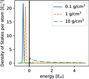
Figure 1: Filled density of states for helium. We have applied an arbitrary broadening of 1 eV to the DOS so that the bound states, which would otherwise be delta functions, can be displayed.

where $n=1,2,\ldots$ The first energy bound for a given $l$, $\epsilon_{x}^{1,l}$ is chosen to be just lower in energy than the lowest energy eigenstate, for that $l$, and $\chi_{x,l}$ is the density of states for excited state $x$ for angular momentum quantum number $l$,

$$\chi_{x,l}(\epsilon)=2(2l+1)\int_{V}d^{3}r|y_{x,\epsilon,l}(r)|^{2}.$$ (27)

With the set of states defined by these energy ranges, we choose to occupy them with all perturbations of integer occupations as is common in atomic physics approaches. We must also choose a maximum $n$ to consider. The quantity $n$ becomes equivalent to the principle quantum number for bound states that are well contained inside the ion-sphere. Hence, for example, if we have a helium plasma, and consider the maximum $n$ to be 2 ($n_{max}=2$), we would have the following list of excited states:

1. $1s^{2}\,2s^{0}\,2p^{0}$

2. $1s^{1}\,2s^{1}\,2p^{0}$

3. $1s^{1}\,2s^{0}\,2p^{1}$

4. $1s^{0}\,2s^{2}\,2p^{0}$

5. $1s^{0}\,2s^{1}\,2p^{1}$

6. $1s^{0}\,2s^{0}\,2p^{2}$

and for configuration 2, for example, we have $n_{2,\epsilon_{1s},0}=0.5$.

In Figure 1 we show the filled DOS for this example for configuration 1. At low densities the bound state is well contained within the ion sphere and there are no free electrons. As density increases, the $1s$ orbital becomes partially bound, and all two electrons cannot fit into the bound state, so the upper energy limit of this state extends into the continuum, satisfying the definition (26). For the highest density, there are no bound states and the $1s$ is extended into the continuum. We see that this atomic picture of excitations will be best if there are no (or very few) free electrons in the plasma since, in our example, for 10 g/cm³, the two ionized electrons are spread evenly over the $1s$ band, which is only one possible distribution out of infinitely many.

There is another problem with this above approach to excited states – it will be prohibitively expensive for high temperatures, or higher $Z$ materials, where $n_{max}$ must be large. A solution is to treat all states with energies higher than $\epsilon_{x,\epsilon_{x}^{n_{max}+1},l}$ with Fermi-Dirac statistics. The lifetime of excitations of core (deeply bound) states is relatively long, and that for excitations of continuum (free) electrons is much shorter due to collisions. Therefore, it is reasonable to create a set of occupation factors that only include a detailed list of excitations for the core states, and use an average occupation (Fermi-Dirac) for the free electrons, at least for EOS purposes. In the results presented here we have used this approach. For our helium example, the list of excited states increases to include

1. $1s^{1}\,2s^{0}\,2p^{0}$ + FD

2. $1s^{0}\,2s^{1}\,2p^{0}$ + FD

3. $1s^{0}\,2s^{0}\,2p^{1}$ + FD

4. $1s^{0}\,2s^{0}\,2p^{0}$ + FD

where the occupation factors are Fermi-Dirac beyond last energy boundary for each $l$ runs, in principle, to $\infty$.

We note that by using Fermi-Dirac occupation factors in the definition of an excited state, the configurations become dependent on temperature, whereas in the first example, the electronic structure of the configurations and their energies are independent of temperature. For configurations that are independent of temperature, the resulting probabilities (populations) do depend on temperature, but simply, through the free energy ($F_{x}=E_{x}-TS_{x}$) and equation (LABEL:eq_wx).

III.2 Application to Aluminum Plasmas

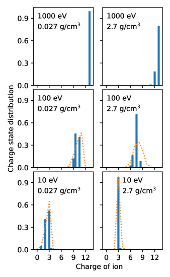
Figure 2: Charge state distributions for aluminum plasmas. We have considered configuration perturbations up to the $n=2$ shell for 2.7 g/cm³, and $n=3$ shell for 0.027 g/cm³. The results of the present model are shown in the blue bars. Also shown with the dotted lines are the results of reference white2022charge .

In Figure 2 the charge state distribution (CSD) for aluminum plasmas is shown. Here we calculate the charge of an ion by counting the number of positive energy electrons, which therefore includes electrons in resonance states. This is a reasonable definition, but we note that with this definition it is possible to have an ion of non-integer charge. This can been seen from Figure 1 where a bound state is partially bound for 1 g/cm³. Physically, this behavior reflects the fact that as a bound state pressure ionizes it is neither truly a bound nor free electron state. In Figure 2 we see that at the highest temperature (1000 eV) and lowest density (0.027 g/cm³), the plasma is fully ionized. Going next to the 1000 eV, 2.7 g/cm³ case, we find that the plasma is mostly fully ionized but contains about 20% of ions with a single bound electron. Increased collisional effects at this higher density are the cause of the lower average ionization.

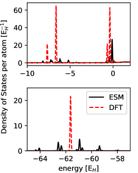
Figure 3: Filled density of states for aluminium at 100 eV and 2.7 g/cm³. The solid black line is the result from the present excited states model (ESM). This is compared to the DFT prediction in dashed red from the average atom model Tartarus starrett19 .

For the 10 and 100 eV cases we compare to the model of White et al. white2022charge , Figure 2. For the 100 eV, 2.7 g/cm³ case the new model is significantly more strongly peaked. For the 2.7 g/cm³ cases we have used $n_{max}=2$. In the limit of using $n_{max}=0$ we would recover the DFT result and the CSD would be peaked at one charge state with all of the population. Using $n_{max}=1$ would allow some fluctuation, $n_{max}=2$ even more, and so on. Hence, the reason why the CSD of the new model is more peaked than that of White et al white2022charge is due to the lower value of $n_{max}$. Does this mean that the result of the present model for this case is not converged with respect to $n_{max}$? As we argued earlier, the present definition of the excited state works best for core states. Using $n_{max}=2$ in this case ensures this outcome, while using $n_{max}=3$ would not as the $n=3$ states are partially bound. Which choice is more reasonable depends on the time scale of the experiment that we wish to model. Excitations of the partially bound $n=3$ states will have a much shorter lifetime than those of the core states. For experiments that probe time-integrated quantities over time-scales that are longer than the $n=3$ excitation lifetimes, the present model is appropriate, whereas, if the experiment has shorter time resolution then considering explicit excitations of these shells would be necessary.

Lastly, we note that the CSD is an output of the model and we are free to choose different definitions of ion charge that are reasonable. This choice does not affect the model in any way – it does not change the EOS, energies, entropy, nor populations.

In Figure 3 the filled density of states is shown for a hot dense aluminum plasma at 100 eV and 2.7 g/cm³ using $n_{max}=2$. With aluminum’s 13 electrons this leads to 63 distinct excited states and the result shown is averaged over all of these with the probabilities $W_{x}$. In the lower panel we see the effect on the $1s$ eigenstate. There are four distinct groupings of $1s$ states. These correspond to four different charge states with significant probability in the plasma. In contrast, we also show the DFT result obtained using the Tartarus code. There is only one peak, corresponding to the average $1s$ energy of the plasma. The different peaks within each cluster correspond to different arrangements of electrons in the ‘spectator’ bound states (i.e., those in the $n=2$ shell), but having the same ion charge.

In the top panel of Figure 3 we again see a cluster of peaks from -10 to -5 E_H corresponding to the $n=2$ shell. The DFT results show two distinct peaks corresponding to the $2s$ and $2p$ eigenstates. Near zero energy, the line corresponding to the $n=3$ states shows up. Since they are not explicitly included in our excited state list, the excited state model predicts a strong line near zero energy.

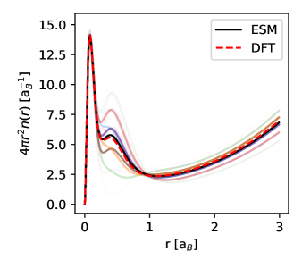
Figure 4: Electron density for aluminium at 100 eV and 2.7 g/cm³. The solid black line is the predicted average radial density from the present excited states model (ESM). This is compared to the DFT prediction in dashed red from the average atom model Tartarus starrett19 . Also shown in semi-transparent lines are the individual densities due to the excited states, with their degree of transparency proportional to to the probability $W_{x}$.

In Figure 4 we show the radial density averaged over all excited states

$$n({\bm{r}})=\sum_{x}W_{x}n_{x}({\bm{r}})$$ (28)

We compare this to the DFT result from the Tartarus model. We find overall good agreement, but some differences are observed. On the one hand, it is not surprising that the average over the excited states is not the same as the averaged excited state. On the other, the difference is fairly small and would be hard to test experimentally. Also shown in the figure are the electron densities from the excited states. These curves indicate that there is little fluctuation in the occupation of $1s$ shell (the peak nearest the origin), there is significant variation on the $n=2$ shell occupation (the second peak from the origin), and significant variation in the free electron density (the tail after the peaks). We note that while the DOS, Figure 3, indicates that the $1s$ eigenvalue does depend on the charge state, Figure 4 shows that these variations do not strongly affect the density due to the $1s$ shell.

In Table 1 the excess pressure is shown (given by equation (24) which does not include the ideal ion contribution) for the same aluminum plasmas, ranging from degenerate systems (2.7 g/cm³ and 10 eV) to fully ionized (0.027 g/cm³ and 1000 eV). These pressures are compared to Tartarus results. Overall agreement is close between the two methods. Agreement is best for the high temperature cases, where details of the interaction potentials are unimportant due to the high average energy of the free electrons, as well as for the most degenerate case, where the plasma is dominated by one charge state (i.e., close to the DFT limit of the model). The remaining differences are relatively small and can be explained by the difference between calculating the pressure of an average system (DFT) versus the average pressure of the resolved excited states.

	Al 0.027 g/cm3
	ESM (n=3)	Tartarus
10 eV	2.02e-2	2.16e-2
100 eV	0.954	0.948
1000 eV	12.5	12.5
	Al 2.7 g/cm3
	ESM (n=2)	Tartarus
10 eV	2.08	2.07
100 eV	64.4	65.4
1000 eV	1203	1201

Table 1: Values of excess pressure in Mbar for aluminum at temperatures of 10, 100 and 1000 eV and densities of 0.027 g/cm³ and 2.7 g/cm³. ESM refers to the present excited states model, while Tartarus refers to the DFT based average atom model starrett19 .

The calculation of $\gamma$ (equation 25) requires an initial guess and an iterative, self-consistent, procedure. We start with the value provided by an average atom model which seems to be close to the final answer. For example, for Al at 100 eV and 2.7 g/cm³, the value from the Tartarus model is $\gamma_{AA}=-0.446$ E_H (which results in a pressure of 64.44 Mbar), while the converged value is $\gamma=-0.444$ E_H (which results in a pressure of 64.41 Mbar). Conveniently, an approximation in which we choose $\gamma$ to vary for each excited state such that $\gamma_{x}=V_{x}^{xc}(R)$, and using $\gamma=\sum_{x}W_{x}\gamma_{x}$ also seems to be accurate for EOS, giving $\gamma=-0.444$ E_H and a pressure of 64.43 Mbar for this case. Clearly, this approximation could be more problematic for excitation energies (differences in excited state energies) than for the EOS which is a more averaged quantity.

IV Conclusions

A variational model of excited states in electronic structure has been presented. The model recovers the usual Kohn-Sham density functional theory approach in the limit where only one state dominates (i.e., for degenerate systems like solids, or for fully ionized plasmas). The model uses an effective one-electron expression for the excited state energy and includes the LDA for the exchange and correlation energy. Boltzmann factors for the excited state probabilities result from minimising the free energy with respect to the probabilities.

Excited states are defined by a set of one-electron level occupation factors. If these are set to be the Fermi-Dirac occupation factors, then Kohn-Sham DFT is recovered. We apply this variational theory to a model of an atom in a plasma; a generalization of the average atom model liberman ; liberman1982inferno . We use an atomic physics-inspired definition of excited states, where permutations of integer occupations of bound states are considered. Comparison of this application to the average atom model Tartarus is made. We see the effect on the density of states, density and pressure. In general the pressure is quite close to the DFT calculation but some differences are observed. Since DFT is a widely used and trusted method, this can be considered as a validation of the current model. The advantage of the current approach is that the calculation of excited states should allow prediction of more realistic optical properties with a consistent and realistic EOS. This advantage remains to be explored.

Appendix A Entropy

The entropy is given by

$$S=-\sum_{i}W_{i}\ln W_{i}$$ (29)

where the sum is over all microstates of the system. If microstate $i$ is degenerate, with $g_{x}$ being the total number of microstates at the energy $E_{x}$, then

$$S=-\sum_{x}\sum_{i\in x}W_{i}\ln W_{i}$$ (30)

the probability of microstate $i$ is $W_{i}=W_{x}/g_{x}$, so

$$\begin{split}S=&-\sum_{x}\sum_{i\in x}\frac{W_{x}}{g_{x}}\ln\frac{W_{x}}{g_{x}}\\ =&-\sum_{x}W_{x}\ln\frac{W_{x}}{g_{x}}\\ =&-\sum_{x}W_{x}\ln W_{x}+\sum_{x}W_{x}S_{x}\\ \end{split}$$ (31)

References

- [1] O. Ciricosta, S. M. Vinko, H-K. Chung, B-I. Cho, C. R. D. Brown, T. Burian, J. Chalupskỳ, K. Engelhorn, R. W. Falcone, C. Graves, et al. Direct measurements of the ionization potential depression in a dense plasma. Physical review letters, 109(6):065002, 2012.
- [2] T. Nagayama, J. E. Bailey, G. P. Loisel, G. S. Dunham, G. A. Rochau, C. Blancard, J. Colgan, Ph. Cossé, G. Faussurier, C. J. Fontes, F. Gilleron, S. B. Hansen, C. A. Iglesias, I. E. Golovkin, D. P. Kilcrease, J. J. MacFarlane, R. C. Mancini, R. M. More, C. Orban, J.-C. Pain, M. E. Sherrill, and B. G. Wilson. Systematic study of L-shell opacity at stellar interior temperatures. Phys. Rev. Lett., 122:235001, Jun 2019.
- [3] James E. Bailey, Taisuke Nagayama, Guillaume Pascal Loisel, Gregory Alan Rochau, C. Blancard, J. Colgan, Ph. Cosse, G. Faussurier, C. J. Fontes, F. Gilleron, et al. A higher-than-predicted measurement of iron opacity at solar interior temperatures. Nature, 517(7532):56–59, 2015.
- [4] Andrea L. Kritcher, Damian C. Swift, Tilo Döppner, Benjamin Bachmann, Lorin X. Benedict, Gilbert W. Collins, Jonathan L. DuBois, Fred Elsner, Gilles Fontaine, Jim A. Gaffney, et al. A measurement of the equation of state of carbon envelopes of white dwarfs. Nature, 584(7819):51–54, 2020.
- [5] L.B. Fletcher, H.J. Lee, T. Döppner, E. Galtier, B. Nagler, P. Heimann, C. Fortmann, S. LePape, T. Ma, M. Millot, et al. Ultrabright x-ray laser scattering for dynamic warm dense matter physics. Nature Photonics, 9(4):274–279, 2015.
- [6] P. Hollebon, O. Ciricosta, M. P. Desjarlais, C. Cacho, C. Spindloe, E. Springate, I. C. E. Turcu, J. S. Wark, and S. M. Vinko. Ab initio simulations and measurements of the free-free opacity in aluminum. Phys. Rev. E, 100:043207, Oct 2019.
- [7] S. M. Vinko, V. Vozda, J. Andreasson, S. Bajt, J. Bielecki, T. Burian, J. Chalupsky, O. Ciricosta, M. P. Desjarlais, H. Fleckenstein, et al. Time-resolved xuv opacity measurements of warm dense aluminum. Physical review letters, 124(22):225002, 2020.
- [8] P. Hakel, M. E. Sherrill, S. Mazevet, J. Abdallah Jr., J. Colgan, D. P. Kilcrease, N. H. Magee, C. J. Fontes, and H. L. Zhang. The new los alamos opacity code ATOMIC. Journal of Quantitative Spectroscopy and Radiative Transfer, 99(1-3):265–271, 2006.
- [9] James Colgan, David P. Kilcrease, N. H. Magee, Manolo E. Sherrill, J. Abdallah Jr, Peter Hakel, Christopher J. Fontes, Joyce A. Guzik, and K. A. Mussack. A new generation of Los Alamos opacity tables. The Astrophysical Journal, 817(2):116, 2016.
- [10] C. A. Iglesias and F. J. Rogers. Updated OPAL opacities. The astrophysical journal, 464:943, 1996.
- [11] John C. Stewart and Kedar D. Jr. Pyatt. Lowering of Ionization Potentials in Plasmas. ApJ, 144:1203–1211, June 1966.
- [12] Burkhard Militzer and Kevin P. Driver. Development of path integral monte carlo simulations with localized nodal surfaces for second-row elements. Phys. Rev. Lett., 115:176403, Oct 2015.
- [13] Edwin L. Pollock and David M. Ceperley. Simulation of quantum many-body systems by path-integral methods. Physical Review B, 30(5):2555, 1984.
- [14] L. Collins, I. Kwon, J. Kress, N. Troullier, and D. Lynch. Quantum molecular dynamics simulations of hot, dense hydrogen. Phys. Rev. E, 52:6202–6219, Dec 1995.
- [15] S. X. Hu, B. Militzer, V. N. Goncharov, S. Skupsky, et al. First-principles equation-of-state table of deuterium for inertial confinement fusion applications. Physical Review B, 84(22):224109, 2011.
- [16] Bastian Holst, Ronald Redmer, and Michael P. Desjarlais. Thermophysical properties of warm dense hydrogen using quantum molecular dynamics simulations. Physical Review B, 77(18):184201, 2008.
- [17] C. E. Starrett and N. Shaffer. Multiple scattering theory for dense plasmas. Phys. Rev. E, 102:043211, Oct 2020.
- [18] P. Hohenberg and W. Kohn. Inhomogeneous electron gas. Phys. Rev., 136:B864–B871, Nov 1964.
- [19] N. David Mermin. Thermal properties of the inhomogeneous electron gas. Phys. Rev., 137:A1441–A1443, Mar 1965.
- [20] Nathaniel R. Shaffer and Charles E. Starrett. Dense plasma opacity via the multiple-scattering method. Phys. Rev. E, 105:015203, Jan 2022.
- [21] Valentin V Karasiev, SX Hu, Nathaniel R Shaffer, and Gennady Miloshevsky. First-principles study of l-shell iron and chromium opacity at stellar interior temperatures. Physical Review E, 106(6):065202, 2022.
- [22] Nathanael Matthew Gill, Christopher John Fontes, and Charles Edward Starrett. Time-dependent density functional theory applied to average atom opacity. Physical Review E, 103(4):043206, 2021.
- [23] A. Zangwill and Paul Soven. Density-functional approach to local-field effects in finite systems: Photoabsorption in the rare gases. Phys. Rev. A, 21:1561–1572, May 1980.
- [24] Erich Runge and E. K. U. Gross. Density-functional theory for time-dependent systems. Phys. Rev. Lett., 52:997–1000, Mar 1984.
- [25] Andreas K. Theophilou. The energy density functional formalism for excited states. Journal of Physics C: Solid State Physics, 12(24):5419, 1979.
- [26] Eberhardt K. U. Gross, Luiz N. Oliveira, and Walter Kohn. Rayleigh-ritz variational principle for ensembles of fractionally occupied states. Physical Review A, 37(8):2805, 1988.
- [27] Eberhardt K. U. Gross, Luiz N. Oliveira, and Walter Kohn. Density-functional theory for ensembles of fractionally occupied states. i. basic formalism. Physical Review A, 37(8):2809, 1988.
- [28] Luiz Nunes de Oliveira, E. K. U. Gross, and W. Kohn. Density-functional theory for ensembles of fractionally occupied states. ii. application to the he atom. Physical Review A, 37(8):2821, 1988.
- [29] Carsten A. Ullrich. Time-dependent density-functional theory: concepts and applications. 2011.
- [30] Carsten A. Ullrich. Time-dependent density-functional theory: features and challenges, with a special view on matter under extreme conditions. In Frontiers and Challenges in Warm Dense Matter, pages 1–23. Springer, 2014.
- [31] Neepa T. Maitra, Fan Zhang, Robert J. Cave, and Kieron Burke. Double excitations within time-dependent density functional theory linear response. The Journal of Chemical Physics, 120(13):5932–5937, 2004.
- [32] Carsten A. Ullrich. Time-dependent density-functional theory beyond the adiabatic approximation: Insights from a two-electron model system. The Journal of chemical physics, 125(23), 2006.
- [33] Davide Sangalli, Pina Romaniello, Giovanni Onida, and Andrea Marini. Double excitations in correlated systems: A many–body approach. The Journal of chemical physics, 134(3), 2011.
- [34] Peter Elliott, Sharma Goldson, Chris Canahui, and Neepa T. Maitra. Perspectives on double-excitations in TDDFT. Chemical Physics, 391(1):110–119, 2011.
- [35] Walter Kohn. Density-functional theory for excited states in a quasi-local-density approximation. Physical Review A, 34(2):737, 1986.
- [36] Nikitas I. Gidopoulos, Petros G. Papaconstantinou, and Eberhardt K. U. Gross. Spurious interactions, and their correction, in the ensemble-kohn-sham scheme for excited states. Physical review letters, 88(3):033003, 2002.
- [37] W. Kohn and L. J. Sham. Self-consistent equations including exchange and correlation effects. Physical review, 140(4A):A1133, 1965.
- [38] Crystal F. Ottoway, Daniel A. Rehn, Didier Saumon, and Charles Edward Starrett. Effect of ionic disorder on the principal shock hugoniot. Physical Review E, 104(5):055208, 2021.
- [39] Mandy Bethkenhagen, Abhiraj Sharma, Phanish Suryanarayana, John E Pask, Babak Sadigh, and Sebastien Hamel. Properties of carbon up to 10 million kelvin from kohn-sham density functional theory molecular dynamics. Physical Review E, 107(1):015306, 2023.
- [40] A. Gonis and M. Däne. Extension of the kohn-sham formulation of density functional theory to finite temperature. Journal of Physics and Chemistry of Solids, 116:86–99, 2018.
- [41] D. H. Sampson, H.L. Zhang, and C. J. F. Fontes. A fully relativistic approach for calculating atomic spectra for highly charged ions. Phys. Rep., 477:111, 2009.
- [42] C. J. Fontes, H. L. Zhang, J. Abdallah Jr., R. E. H. Clark, D. P. Kilcrease, J. Colgan, R. T. Cunningham, P. Hakel, N. H. Magee, and M. E. Sherrill. The los alamos suite of relativistic atomic physics codes. Journal of Physics B: Atomic, Molecular and Optical Physics, 48(14):144014, 2015.
- [43] N. M. Gill, C. J. Fontes, and C. E. Starrett. A superconfiguration calculation of opacity with consistent bound and continuum electron treatments using green’s functions. Journal of Physics B: Atomic, Molecular and Optical Physics, 56(1):015001, 2023.
- [44] A. Bar-Shalom, J. Oreg, W. H. Goldstein, D. Shvarts, and A. Zigler. Super-transition-arrays: A model for the spectral analysis of hot, dense plasma. Physical Review A, 40(6):3183, 1989.
- [45] T. Blenski and B. Cichocki. Variational approach to the average-atom-in-jellium and superconfigurations-in-jellium models with all electrons treated quantum-mechanically. High Energy Density Physics, 3(1–2):34 – 47, 2007. Radiative Properties of Hot Dense Matter.
- [46] R. Piron and T. Blenski. Variational average-atom in quantum plasmas (vaaqp)–application to radiative properties. High Energy Density Physics, 9(4):702–710, 2013.
- [47] J.-C. Pain, F. Gilleron, Q. Porcherot, T. Blenski, and Djamel Benredjem. The hybrid detailed / statistical opacity code sco-rcg: New developments and applications. AIP Conference Proceedings, 1811(1):190010, 2017.
- [48] David A. Liberman. Self-consistent field model for condensed matter. Phys. Rev. B, 20:4981–4989, Dec 1979.
- [49] David A. Liberman. INFERNO: A better model of atoms in dense plasmas. Journal of Quantitative Spectroscopy and Radiative Transfer, 27(3):335–339, 1982.
- [50] T. Blenski and K. Ishikawa. Pressure ionization in the spherical ion-cell model of dense plasmas and a pressure formula in the relativistic Pauli approximation. Physical Review E, 51(5):4869, 1995.
- [51] R. Piron and T. Blenski. Variational-average-atom-in-quantum-plasmas (VAAQP) code and virial theorem: Equation-of-state and shock-hugoniot calculations for warm dense Al, Fe, Cu, and Pb. Phys. Rev. E, 83:026403, Feb 2011.
- [52] J. R. White, W. Johns, C. J. Fontes, N. M. Gill, N. R. Shaffer, and C. E. Starrett. Charge state distributions in dense plasmas. Physics of Plasmas, 29(4):043301, 2022.
- [53] C. E. Starrett, N. M. Gill, T. Sjostrom, and C. W. Greeff. Wide ranging equation of state with tartarus: A hybrid green’s function/orbital based average atom code. Computer Physics Communications, 235:50 – 62, 2019.