General Relativistic Chronometry with Clocks on Ground and in Space

Abstract

One of geodesy’s main tasks is to determine the gravity field of the Earth. High precision clocks have the potential to provide a new tool in a global determination of the Earth’s gravitational potential based on the gravitational redshift. Towards this clock-based gravimetry or chronometry in stationary spacetimes, exact expressions for the relativistic redshift and the timing between observers in various configurations are derived. These observers are assumed to be equipped with standard clocks and move along arbitrary worldlines. It is shown that redshift measurements, involving clocks on ground and/or in space, can be used to determine the (mass) multipole moments of the underlying spacetime. Results shown here are in agreement with the Newtonian potential determination from, e.g., the so-called energy approach. The framework of chronometric geodesy is exemplified in different exact vacuum spacetimes for illustration and future gravity field recovery missions may use clock comparisons as an additional data channel for advanced data fusion.

I Introduction

One main task of geodesy is to determine the gravitational field and orientation of the Earth. The conventional way to achieve this is by using gravimeters, gradiometers, gyroscopes, as well as astronomical observations. Significant progress in the development of highly accurate clocks allows to leverage the general relativistic effect of the gravitational redshift for probing gravitational fields. This has been proposed for the first time by Bjerhammar Bjerhammar (1985), and due to the present stability of atomic clocks of $10^{-18}$ Mehlstäubler et al. (2018) one can resolve the Newtonian gravitational potential at the level of one centimeter. Since the comparison of clocks with optical fibers is at least one order of magnitude more stable than free-space links Droste et al. (2013) one may determine the gravitational potential even on large scales. For a global determination of the gravitational potential, however, satellites have to be used either as transmitters or as instruments equipped with stable clocks. Such clocks onboard of satellites can be used to disseminate time and frequency around the world, or they can be used as devices to determine the gravitational potential in space. To develop the theoretical foundation of the latter is the purpose of this article, for which the formalism of General Relativity (GR) is employed without resorting to post-Newtonian approximations.

In Philipp et al. (2017, 2020) a general relativistic, i.e., chronometric formulation of the gravitational field of the Earth is given. It is mainly based on the assumption that the field (in the mean) is stationary and clocks are not moving with respect to the rotating Earth. The formalism allows to define a fully general relativistic geoid and it is shown that the equipotential surfaces defined by clock comparisons coincide with the equipotential surfaces defined by usual gravimeters and gradiometers such as as falling corner cubes or atomic interferometers. For chronometry with satellites we have to modify the formalism in order to allow for the integration of moving clocks. This will be achieved in the present article.

The clock comparison between Earth-bound clocks and satellites via electromagnetic signals propagating through the Earth’s atmosphere is not as stable as the comparison done by using optical fibers, which link clocks on the Earth’s surface. The stability is typically of the order $10^{-15}$ and not better than $10^{-16}$. Accordingly, in order to do chronometry in space, it might be beneficial to pairwise compare clocks in space directly to determine the gravitational potential there and conclude it’s global characteristics.

In the first part of the paper, the main theoretical notions are introduced and the problem is rigorously defined. In the second part general results for space and ground-based chronometry are derived. This includes the discussion of clocks on satellites, moving on geodesics or on arbitrary worldlines, as well as clocks on ground, which are located on, e.g., the relativistic geoid. It is shown how pairwise redshift measurements can be used to determine level surfaces of a relativistic gravity potential, which in general depends on the multipole moments of the underlying spacetime. The last part contains a brief discussion of the results in special, analytically given spacetimes for illustration and for clarifying the notions.

II Status of clock comparison

Clock comparison is governed by Special Relativity (SR) as well as GR. SR describes the Doppler effect (longitudinal and transversal) and GR adds the gravitational redshift and the gravitational time delay. The Doppler effect describes the dependence of the difference in measured ticking rates of clocks on the relative motion, and the gravitational redshift introduces the dependence on their relative positions. The time delay is an effect due to the propagation of signals in the gravitational field.

The first experiment testing the gravitational redshift was done by Pound and Rebka in 1960 Pound and Rebka (1960). The authors verified the change of a photon’s frequency during propagation in the gravitational field of the Earth. In 1966, the GEOS-1 satellite was used to observe the relativistic Doppler effects Jenkins (1969). In 1976, the famous Gravity Probe A (GPA) experiment was conducted Vessot and Levine (1979); Vessot et al. (1980); Vessot (1989). Two hydrogen masers, one of which was carried to a height of about $10^{4}\,$km by a Scout D rocket, were compared.  To quote from the results of this seminal experiment Vessot et al. (1980): “The agreement of the observed relativistic frequency shift with prediction is at the $70\times 10^{-6}$ level.” The gravitational redshift, however, was confirmed with an accuracy of $1.4\times 10^{-4}$, see Ref. Vessot (1989). At present, the best result and highest accuracy of the gravitational redshift is achieved by analyzing clock data from the Galileo satellites 5 and 6, which were launched into elliptic orbits due to a malfunction of the rocket’s upper stage. This coincidence reduced the satellites usefulness for navigation but made them ideal tools for tests of GR. The data analysis and integration over (at least) one year improved the GPA limit to about $4\times 10^{-5}$ Herrmann et al. (2018); Delva et al. (2018). The upcoming Atomic Clock Ensemble in Space (ACES) proposes to test the gravitational redshift at the $10^{-6}$ level Heß et al. (2011); Cacciapuoti and Salomon (2009); Savalle et al. (2019), aiming for another magnitude of improved accuracy.

In the past, several satellite-based tests of SR and GR that involve space-based clocks have been proposed, see, e.g., Lämmerzahl et al. (2001); Dittus et al. (2007). A recent approach to test the GR prediction of the gravitational redshift uses the RadioAstron satellite and the authors are confident to reach an accuracy in the $10^{-5}$ regime Litvinov et al. (2017). Further prospects for future satellite missions using spacecraft clocks are discussed in, e.g., Angélil et al. (2014) and Altschul et al. (2015).

For a general overview of ”The Confrontation between General Relativity and Experiment“, we refer the reader to the living review article Will (2006). Details on relativistic effects in the Global Positioning System (GPS), in particular on satellite timing and the Earth–to–satellite redshift, can be found in the review Ashby (2003), and references therein. For time transfer in the vicinity of the Earth and general definitions of different time scales we refer to Nelson (2011).

Relativistic redshift effects can also serve to test different theories of gravity Bondarescu et al. (2015); Jetzer (2017). For instance, scalar-tensor theories and their parametrized post-Newtonian form were considered in Ref. Schärer et al. (2014), in which the authors consider the difference to the GR redshift signals for artificial satellite orbits around the Earth.

All the achievements and considerations mentioned so far do (usually) only take into account the first order post-Newtonian approximation of the relativistic redshift, which contains the Doppler effect and the gravitational redshift to order $\mathcal{O}\big{(}1/c^{2}\big{)}$. This may be sufficient to meet present technological capabilities and to provide the theoretical framework for clocks in space with contemporary accuracy for frequency transfer related to modern IAU and IERS conventions. However, in order to construct a fully relativistic framework for future high-precision experiments in a top-down approach, and to obtain a thorough understanding and interpretation of measurement results we find it necessary to investigate all related notions in GR without approximation. Thus, in this work we formulate exact expressions for the general relativistic redshift in stationary spacetimes. Based on the results, weak-field approximations in, e.g., the post-Newtonian framework are derived. While stationarity can be regarded as a strong assumption though, it is important to note that this assumption holds true in the exterior of the Earth for a significant duration, spanning multiple satellite orbit closures. Any dynamics can be subsequently included into the analysis in an adiabatic manner.

III Setting

III.1 Geometry, notation and redshift definition

We use Einstein’s summation convention, Greek indices are spacetime indices and run from 0 to 3, and Latin indices are purely spatial indices running from 1 to 3. Our metric signature convention is $(-,+,+,+)$. If not noted otherwise, we use the framework of Einstein’s GR and assume the vacuum field equation to be fulfilled.

As an illustrative example, the comparison of clocks in the space surrounding Earth is considered. However, it’s crucial to emphasize that the outcomes of such comparisons are universally applicable to any other stationary spacetime.

Let ${(\mathcal{M},g)}$ be the relativistic spacetime manifold with metric $g$, for which we assume stationarity, and let $\nabla$ be the Levi-Civita covariant derivative of $g$.

A light signal (null geodesic or optical fiber-guided) is described by a null curve $\lambda$ on $\mathcal{M}$,

$$\lambda:\mathbb{R} \to\mathcal{M}$$

$$s \mapsto\lambda(s)\,,$$ (1)

where $s$ is an affine parameter along the curve. The tangent vector to the worldline is denoted by $l:=\mathrm{d}\lambda/\mathrm{d}s$ with

$$g(l,l)=0\,,$$ (2)

and it is related to a wave covector $k$ via

$$l=g^{-1}(k,\cdot)\,,$$ (3)

where $g^{-1}$ is the inverse metric.

The worldline of an observer is the image of a map $\gamma$,

$$\gamma:\mathbb{R} \to\mathcal{M}$$

$$\tau \mapsto\gamma(\tau)\,,$$ (4)

with a normalization

$$g(u,u)=-c^{2}\,,\quad u:=\dot{\gamma}:=\dfrac{\mathrm{d}\gamma}{\mathrm{d}\tau}\,,$$ (5)

that holds along the worldline for the future-pointing tangent $u$. The curve parameter $\tau$ is called proper time. Clocks which show proper time along their worldlines are called standard clocks. They can be characterized operationally as shown in Perlick (1987).

In a chart $(\mathcal{U},x)$, with domain $U\subset\mathcal{M}$ and coordinate map $x:\mathcal{M}\to\mathbb{R}^{4}$, the components are

$$l^{\mu} =\dfrac{\mathrm{d}(x\circ\lambda)^{\mu}}{\mathrm{d}s}\,,\quad k_{\mu}=g_{\mu\nu}l^{\nu}\,,u^{\mu} =\dfrac{\mathrm{d}(x\circ\gamma)^{\mu}}{\mathrm{d}\tau}\,.$$ (6a)

and the elapsed proper time along a clock’s worldline is

$$\tau=\dfrac{1}{c}\int_{\gamma}\sqrt{g_{\mu\nu}\mathrm{d}x^{\mu}\mathrm{d}x^{\nu}}\,.$$ (7)

A given observer associates a momentary frequency $\nu_{p}$ with a light ray at the event at which their worldlines intersect, ${p\in\mathcal{M}:=\operatorname{img}(\gamma)\cap\operatorname{img}(\lambda)}$, where $\operatorname{img}(\cdot)$ denotes a map’s image. The frequency of a photon at such an event is the map

$$\nu_{p}:T_{p}\mathcal{M}\supset\mathcal{A}_{p} \to\mathbb{R}$$

$$u \mapsto\nu_{p}(u):=k(u)\big{|}_{p}\,.$$ (8)

Here, $\mathcal{A}_{p}$ is the set of all timelike, future-pointing, and normalized four-velocities in $T_{p}\mathcal{M}$. Hence, the frequency of the photon is not determined until an observer is chosen. At $p$, the respective curve parameters are $s_{p}$ and $\tau_{p}$, such that

$$\lambda(s_{p}):=p=:\gamma(\tau_{p})\,.$$ (9)

The affine parameter can always be chosen such that ${s_{p}=0}$ and we can scale ${\tau_{p}=0}$ as well for a single event of interest (offset the clock’s dial). For the sake of simplicity, also the coordinate time $t_{p}:=t|_{p}$ can be set to zero.

Now, consider (at least) two distinct observers, whose worldlines intersect the same null geodesic. Let them be described by their respective normalized four-velocities $u$ and $\tilde{u}$, with worldlines (integral curves) $\gamma(\tau)$ and $\tilde{\gamma}(\tilde{\tau})$. The redshift $z$ between them is defined by the quotient of emission and reception time increments,

$$z+1:=\underset{{\Delta\tau\to 0}}{\mathrm{lim}}\dfrac{\Delta\tilde{\tau}}{\Delta\tau}=\dfrac{d\tilde{\tau}}{d\tau}\,,$$ (10)

see the sketch in Fig. 1.

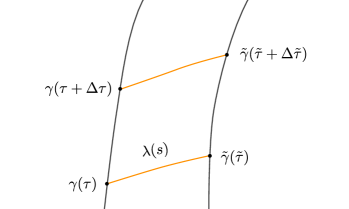
Figure 1: Sketch of the signal transmission between emitter and receiver for the definition of the redshift. Two worldlines $\gamma$ and $\tilde{\gamma}$ with tangent vectors $u$ and $\tilde{u}$ are given. The successive exchange of lightlike signals gives rise to the definition of the redshift $z$ according to Eq. (10).

In GR, there is a universal formula for the redshift in Eq. (10), which is Kermack et al. (1934)

$$z =\dfrac{\nu_{p}(u)}{\nu_{\tilde{p}}(\tilde{u})}-1=\dfrac{k(u)\big{|}_{p}}{k(\tilde{u})\big{|}_{\tilde{p}}}-1\,,$$ (11)

where

1. $k$ is the wave covector field of the null geodesic $\lambda$ that intersects the observers’ worldlines,

2. $p=\operatorname{img}(\gamma)\cap\operatorname{img}(\lambda)$,

3. $\tilde{p}=\operatorname{img}(\tilde{\gamma})\cap\operatorname{img}(\lambda)$.

Note that no metric is needed to define the redshift and the affine parameter along the light ray can always be scaled such that

$$\lambda(0)=\lambda(s_{p})=p=\gamma(\tau_{p})\,,\quad\lambda(1)=\lambda(s_{\tilde{p}})=\tilde{p}=\tilde{\gamma}(\tilde{\tau}_{\tilde{p}})\,.$$ (12)

Hence, the affine parameter runs from 0 to 1 between emission and reception. Note that for geodesic signals $\tilde{p}$ is on the (future) light cone of $p$ and we restrict all considerations to situations in which exactly one null geodesic exists that connects the two events. This is certainly true for compact objects like the Earth and even for Neutron Stars, but not in the immediate vicinity of objects like black holes allowing a photon sphere.

III.2 Emitter–observer maps

The three quantities $u,\tilde{u},k$ are, in general, not independent. For two observers $\gamma,\tilde{\gamma}$, we may choose $p\in\text{img}(\gamma)$ as an emission event. Then, this choice (uniquely) determines $k$ and $\tilde{p}$ such that the null geodesic starting at $p$ with initial condition $k|_{p}$ intersects $\operatorname{img}(\tilde{\gamma})$ at $\tilde{p}$. Thus, the event of reception is a function of the event of emission, i.e., $\tilde{p}=\tilde{p}(p)$. The redshift may then be parametrized by either the time of emission or the time of reception and the emitter-observer problem (EOP) is hidden here implicitly. It consists in finding the light ray $\lambda$ that fulfills Eq. (12) for given observer worldlines and a chosen emission event. No analytic solution to this problem is known (yet), even in simple spacetimes, but there exist approximation schemes Semerák (2015).

However, it is instructive to view the redshift from a slightly different perspective as a map from $\mathbb{R}\to\mathbb{R}$ in the following way. Let

$$\Lambda:\text{img}(\gamma) \to\text{img}(\tilde{\gamma})$$

$$p \mapsto\Lambda(p):=h^{l_{p}}_{1}(p)=\tilde{p}$$ (13)

be called the emitter–observer (EO) event map, such that (12) holds with a connecting light ray $\lambda$, which has the tangent $l_{p}=g^{-1}(k,\cdot)|_{p}$ at $p$. $\Lambda$ maps $p$ to $\tilde{p}$ along the (geodesic) flow of $l_{p}$ for unit parameter distance. In a chart, of which the domain covers the experiment, $\Lambda$ has a representative

$$\bar{\Lambda}=x\circ\Lambda\circ x^{-1}:\mathbb{R}^{4}\supset x(\operatorname{img}(\gamma)) \to x(\operatorname{img}(\tilde{\gamma}))\subset\mathbb{R}^{4}$$

$$x(p) \mapsto x(\tilde{p})\,.$$ (14)

Because $\gamma$ and $\tilde{\gamma}$ are both curves on ${\mathcal{M}}$, we can also define an EO timing map $\Sigma$,

$$\Sigma:=\tilde{\gamma}^{-1}\circ\Lambda\circ\gamma:\mathbb{R}\supset\text{preimg}(\gamma) \to\text{preimg}(\tilde{\gamma})\subset\mathbb{R}$$

$$\tau \mapsto\Sigma(\tau):=\tilde{\tau}\,,$$ (15)

see Fig. 2. Here, $\tau$ is the proper time read off the clock on $\gamma$ at the emission of the signal and $\Sigma(\tau)=\tilde{\tau}$ is the proper time read off the clock on $\tilde{\gamma}$ at reception of the signal. Since for a map from ${\mathbb{R}\to\mathbb{R}}$ we clearly understand the derivative, we can now define the redshift as a function of the emission time by

$$z:=\Sigma^{\prime}-1:\mathbb{R} \to\mathbb{R}$$

$$\tau \mapsto z(\tau):=\Sigma^{\prime}(\tau)-1\,,$$ (16)

where the prime denotes the derivative w.r.t. $\tau$. Hence, all that is needed for the calculation of the redshift is, in principle, the map $\Lambda$ and the EOP is encoded in it. If this map is known (numerically or via an approximate descriptions), the redshift can be calculated easily.

The EO timing map $\Lambda$ is also related to the time transfer function $\mathcal{T}$ in a chart $(\mathcal{U},x)$ with $(x^{\mu})=(t,x^{i})$ by

$$\mathcal{T}(p,\tilde{p}): =x^{t}(\tilde{p})-x^{t}(p)=x^{t}(\Lambda(p))-x^{t}(p)$$

$$=(x\circ\Lambda)^{t}(p)-x^{t}(p)=\bar{\Lambda}^{t}(x(p))-x^{t}(p)\,.$$ (17)

Hence, the chart-dependent time transfer function is included in the chart components of $\Lambda$.

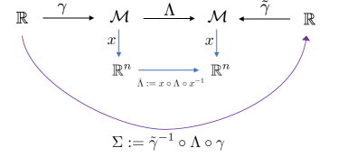
Figure 2: The emitter-observer maps definitions.

However, the total redshift will in general contain contributions from the geometry of the spacetime and from the Doppler effect known from SR due to relative motion. The redshift equation(11) can now be rewritten as

$$z(\tau)=\dfrac{k(u)\big{|}_{p}}{k(\Lambda^{*}(u))\big{|}_{\Lambda(p)}}-1\,,$$ (18)

where $u=u(\tau)$ and $\Lambda^{*}$ is the push-forward defined w.r.t. the map $\Lambda$ . This notation clearly demonstrates that the reception event is a direct function of the emission event, effectively encapsulating the essence of the EOP. Note that tangent vectors of curves are pushed forward to tangent vectors of the image curves, which are constructed by the underlying flow, i.e., here we have $\tilde{u}=\Lambda^{*}(u)$.

In the chart, the redshift can then be decomposed into

$$z(\tau)+1 =\dfrac{k_{t}(0)u^{t}+k_{i}u^{i}\big{|}_{p}}{k_{t}(1)\tilde{u}^{t}+k_{i}\tilde{u}^{i}\big{|}_{\Lambda(p)}}$$

$$=\dfrac{u^{t}(\tau)+\dfrac{k_{i}(0)}{k_{t}}u^{i}(\tau)}{\tilde{u}^{t}\big{(}\Sigma(\tau)\big{)}+\dfrac{k_{i}(1)}{k_{t}}\tilde{u}^{i}\big{(}\Sigma(\tau)\big{)}}$$ (19)

because in a stationary spacetime with adapted coordinates chosen $k_{t}$ is a constant of motion along the null geodesic. The wave covector $k$ at emission and reception is given by the respective derivative of the time transfer function,

$$\dfrac{k_{i}(0)}{k_{t}}=c\dfrac{\partial\mathcal{T}(p,\tilde{p})}{\partial x^{i}}\,,\quad\dfrac{k_{i}(1)}{k_{t}}=-c\dfrac{\partial\mathcal{T}(p,\tilde{p})}{\partial\tilde{x}^{i}}\,,$$ (20)

Thus, the redshift can also be written as

$$z(\tau)+1=\dfrac{u^{t}(\tau)+c\dfrac{\partial\mathcal{T}(p,\tilde{p})}{\partial x^{i}}u^{i}(\tau)}{\tilde{u}^{t}\big{(}\Sigma(\tau)\big{)}-c\dfrac{\partial\mathcal{T}(p,\tilde{p})}{\partial\tilde{x}^{i}}\tilde{u}^{i}\big{(}\Sigma(\tau)\big{)}}\,,$$ (21)

which demonstrates, again, in combination with Eqs. (III.2) and (III.2) that all the information is, in principle, contained in the EO map $\Lambda$. Hence, to calculate or model the redshift between given observer worldlines, there are several equivalent expressions available as outlined above.

In studies such as RELAGAL and GREAT Herrmann et al. (2018); Delva et al. (2015), which analyze the redshift of satellites w.r.t. Earth-bound clocks, usually clock residuals instead of redshifts are investigated. This can be done by relating the proper times $\tau$ and $\tilde{\tau}$ using Eq. (10). Thus,

$$\mathrm{d}\tilde{\tau}=\mathrm{d}\tau\,(z+1)\,,$$ (22)

and, therefore,

$$\tilde{\tau}=\Sigma(\tau)=\tau+\int_{\gamma}z(\tau)\,\mathrm{d}\tau+\mathcal{C}\,,$$ (23)

with some constant offset $\mathcal{C}$. Measured clock residuals along a satellite’s orbit can then be used to calculate the redshift, which is compared to models for tests of GR and other theories of gravity.

In the Newtonian limit, we have $\Sigma(\tau)=\tau+\mathcal{C}$ and, thus, $z=\Sigma^{\prime}=0$ as time is absolute and there is no redshift.

For two stationary observers in a stationary spacetime we have

$$\Sigma(\tau)=\mathcal{C}_{1}(p,\tilde{p})\,\tau+\mathcal{C}_{0}\,.$$ (24)

Thus, the redshift is constant but position dependent and given by

$$z=\mathcal{C}_{1}(p,\tilde{p})\,,$$ (25)

which relates to the existence of a time-independent redshift potential, see below.

A precise description of the involved EOP can now be formulated as follows. Given observers $\gamma$ and $\tilde{\gamma}$, the EOP consist in finding for every event $p$ on the emitter’s worldline a null vector $l_{p}$ such that

$$\operatorname{img}(\tilde{\gamma})\equiv\left\{\tilde{p}=h^{l_{p}}_{1}(p)\,\,\forall p\in\text{img}(\gamma)\right\}\,.$$ (26)

The most difficult step in the theoretical redshift modeling is to solve the EOP. To this end, we can consider some kind of approximate or intermediate modeling in the following way. Parametrize the worldlines of both observers by coordinate time. Choose any $p\in\operatorname{img}(\gamma)$ as an emission event and let $x^{t}(p)=t(p)$ be the coordinate emission time. We start with the simultaneity approximation and solve the geodesic equation for the light ray between the spatial positions related to $p=\gamma(t)$ and $\tilde{p}=\tilde{\gamma}(t)$, which is a boundary value problem. For this signal, a travel time $\Delta t$ can be calculated and leads to a better position estimate of the receiver, which is $\tilde{\gamma}(t+\Delta t)$. Again, the signal is modeled between the emission event and the new reception event. For the new signal, a travel time is calculated and the procedure is repeated until a predefined convergence criterion is met.

III.3 Metric, observers, and velocities

Consider two observers as introduced above and let them exchange light signals. So far, neither of them needs to be geodesic or distinguished in any way.

A general stationary spacetime can be described by the metric

$$g=g_{tt}\mathrm{d}t^{2}+2g_{ti}\mathrm{d}t\mathrm{d}x^{i}+g_{ij}\mathrm{d}x^{i}\mathrm{d}x^{j},$$ (27)

where we use coordinates $(t,x^{i})$ and assume that the time-coordinate $t$ is adapted to the symmetry such that $\partial_{t}$ is the timelike Killing vector field. Then, we can write

$$g_{tt}=-c^{2}e^{2\phi}$$ (28)

with the gravitational redshift potential $\phi$, which is constant along the trajectory of stationary observers Ehlers (1993); Hasse and Perlick (1988) and which is the basis for so-called gravito-electric effects and derived notions, e.g., the definition of the relativistic geoid and heights Philipp et al. (2017, 2020). Far away from the gravitating source we have $g_{tt}\to-c^{2}$. Level surfaces of $\phi$ are called isochronometric, i.e., two stationary clocks (clocks on $t-$lines) on the same level surface have a vanishing redshift Philipp et al. (2017, 2020). Alternatively, the metric can also be written as

$$g=-e^{2\phi}\left(c\mathrm{d}t+\sigma_{i}\mathrm{d}x^{i}\right)^{2}+e^{-2\phi}\gamma_{ij}\,\mathrm{d}x^{i}\mathrm{d}x^{j}\,,$$ (29)

and $\gamma_{ij}$ is the spatial metric seen by the Killing observers. All gravitational degrees of freedom are encoded in $\phi$, $\sigma_{i}$, and $\gamma_{ij}$. The gravitomagnetic degrees of freedom, $\sigma_{i}$, can further be related to the twist potential $\omega$,

$$\partial_{i}\omega=-e^{2\phi}\epsilon_{ijk}D^{j}\sigma^{k}\,,$$ (30)

where $D$ is the covariant derivative w.r.t. $\gamma_{ij}$. In total, there are ten degrees of freedom but note also that four can be eliminated by coordinate transformations.

For Killing observers at a coordinate position ${x:=(x^{i})}$, the relation between proper time and coordinate time is

$$\mathrm{d}t=e^{-\phi(x)}\mathrm{d}\tau\quad\Leftrightarrow\quad u^{t}_{\text{Killing}}=e^{-\phi(x)}\,.$$ (31)

From the normalization of an arbitrary observer’s four-velocity we have

$$-c^{2}=g_{tt}\big{(}u^{t}\big{)}^{2}+2g_{ti}u^{t}u^{i}+g_{ij}u^{i}u^{j}\,,$$ (32)

and only the spatial velocity components are, in principle, subject to measurement. We can express $u^{t}$ as a function of $u^{i}$,

$$u^{t}=\dfrac{\sigma_{i}u^{i}}{c}+e^{-\phi}\sqrt{e^{2\phi}\left(\dfrac{\sigma_{i}u^{i}}{c}\right)^{2}+1+\dfrac{u^{2}}{c^{2}}}\,,$$ (33)

where $u^{2}:=g_{ij}u^{i}u^{j}$. In the static limit ($g_{ti}\to 0$), this reduces to

$$u^{t}=e^{-\phi}\sqrt{1+u^{2}/c^{2}}\,.$$ (34)

Let the coordinate velocities $v^{i}$ be defined by

$$v^{i}:=\dfrac{\mathrm{d}x^{i}}{\mathrm{d}t}\quad\Rightarrow\quad u^{i}=v^{i}\,u^{t}\,,$$ (35)

and, thus, the normalization leads to

$$u^{t}=\dfrac{e^{-\phi}}{\sqrt{1+\dfrac{2\sigma_{i}v^{i}}{c}-e^{-2\phi}\dfrac{v^{2}}{c^{2}}}}\,,$$ (36)

where $v^{2}:=g_{ij}v^{i}v^{j}$. In the static limit, $u^{t}$ is given by

$$u^{t}=\dfrac{e^{-\phi}}{\sqrt{1-e^{-2\phi}\dfrac{v^{2}}{c^{2}}}}\,.$$ (37)

Note that the above equation resembles a modified Lorentz factor and in the special relativistic limit $\exp(-\phi)\to 1$.

We can introduce yet another velocity $w^{i}$, which is defined by a stationary standard clock at an observer’s momentary position $x$

$$w^{i}:=\dfrac{\mathrm{d}x^{i}}{\mathrm{d}\tau_{s}}=\dfrac{\mathrm{d}x^{i}}{\mathrm{d}t}\dfrac{\mathrm{d}t}{\mathrm{d}\tau_{s}}=v^{i}e^{-\phi(x)}\,.$$ (38)

Here $\tau_{s}$ is the proper time on the locally stationary standard clock at $x$ and we observe that

$$\phi(x)=-\log\left(\dfrac{w^{i}}{v^{i}}\right)\,.$$ (39)

Thus, observing the velocity of a satellite on the two time scales $t$ and $\tau_{s}$ allows, in principle, to determine the metric function $\phi(x)$ locally. However, the coordinate time scale $t$ is, unfortunately, not accessible in experiments.

In total we have three different velocities $u^{i},v^{i},w^{i}$, related to three different time scales. They serve to simplify equations, take another viewpoint on the problem, and are beneficial for specific applications, respectively.

IV Redshift and gravity level surfaces

One application of redshift measurements is to determine level sets (i.e., equipontential surfaces) of a relativistic gravity potential $U^{*}$.

$$U^{*}:=c^{2}\left(e^{\phi}-1\right)\,.$$ (40)

It is derived from the redshift potential $\phi$ and also realizes the relativistic geoid in terms of a particular level surface Philipp et al. (2020). This potential is of great importance for chronometry and relativistic geodesy in general. Level surfaces of $\phi$ are also level surfaces of $U^{*}$ and in the weak-field limit $U^{*}\to W$, where $W$ is the Newtonian gravity potential used in conventional geodesy.

The determination of level surfaces allows to infer the spacetime’s multipole moment structure and, thus, the underlying geometry. The mass moments are important for, e.g., height references, global unified height systems, as well as navigation and positioning. This adds yet another – chronometric – data channel to conventional gravity field recovery and experiments such as GOCE and GRACE, which determine the Earth’s (Newtonian) gravity field but the approach here is entirely formulated within GR.

In the special case that one of the two observers, say $\tilde{\gamma}$, is stationary, i.e., at rest on a $t$-line we have

$$1+z(\tau)=e^{\phi_{0}}\left(u^{t}(\tau)+\dfrac{k_{i}(0)}{k_{t}}u^{i}(\tau)\right)\,,$$ (41)

where $\phi_{0}=\phi|_{\tilde{p}}$ is the value of the redshift potential at the stationary observer’s position. We may think of an Earth-bound clock positioned on the geoid such that the adapted coordinate system is co-rotating with the Earth. The equation above can be used to theoretically model the redshift between an Earth-bound clock and a clock onboard a moving satellite but it is not suited for comparisons to real observations because the four-velocity $u$ can not be directly measured.

The well-known limit for two stationary observers, e.g., two clocks on the Earth’s surface, follows immediately,

$$1+z=\dfrac{u^{t}}{\tilde{u}^{t}}=e^{\phi|_{\tilde{p}}-\phi|_{p}}=:e^{\Delta\phi}\,,$$ (42)

which is the constant $\mathcal{C}_{1}$ in (25). This equation is the basis to model the comparison of any two stationary Earth-bound clocks linked by, e.g., optical fiber networks Mehlstäubler et al. (2018); Philipp et al. (2017).

If the velocities $u,\tilde{u}$ are known for moving clocks, analytical models of the redshift can be constructed, given the solution to the EOP. Using the normalization (32) to eliminate $u^{t}$ and $\tilde{u}^{t}$ in the redshift equation (III.2) allows to write the solutions as a function of the spatial velocities. In the static limit the redshift can be given in a compact form,

$$1+z=\dfrac{e^{-\phi(x)}\sqrt{1+u(\tau)^{2}/c^{2}}+\dfrac{k_{i}(0)u^{i}(\tau)}{k_{t}}}{e^{-\phi(\tilde{x})}\sqrt{1+\tilde{u}(\Sigma(\tau))^{2}/c^{2}}+\dfrac{k_{i}(1)\tilde{u}^{i}(\Sigma(\tau))}{k_{t}}}\,.$$ (43)

The stationary pendant looks more complicated but follows straightforwardly from (32) and (III.2).

However, the four-velocities $u,\tilde{u}$ are not measured in real observations anyway. Rather the coordinate velocities $v^{i}$ may be used to proceed. Then, the coordinate time $t$ parameterizes the redshift and the formula neatly factorizes into

$$1+z(t)=\dfrac{u^{t}(t)}{\tilde{u}^{t}(\tilde{t})}\dfrac{\left(1+\dfrac{k_{i}(0)v^{i}(t)}{k_{t}}\right)}{\left(1+\dfrac{k_{i}(1)\tilde{v}^{i}(\tilde{t})}{k_{t}}\right)}\,,$$ (44)

where the signal reception time is ${\tilde{t}=\bar{\Lambda}^{t}(x(t))}$ and ${x(t):=x\circ\gamma(t)}$ is the emission event in the chart with emission time $t$. The second factor in (44) describes the longitudinal (linear) part of the Doppler effect. It is proportional to the line-of-sight projection of the observers’ coordinate velocities and will be abbreviated in the following by

$$\mathcal{D}(t,\tilde{t}):=\dfrac{1+\dfrac{k_{i}(0)}{k_{t}}v^{i}(t)}{1+\dfrac{k_{j}(1)}{k_{t}}\tilde{v}^{j}(\tilde{t})}\,.$$ (45)

The first factor in (44) contains the gravitational (geometric) contribution and the transversal part of the Doppler effect. Inserting $u^{t}$ and $\tilde{u}^{t}$ from Eq. (36) leads to

$$1+z\\ =e^{\Delta\phi}\sqrt{\dfrac{\sigma_{i}(\tilde{x})\tilde{v}^{i}(\tilde{t})/c+1-e^{-2\phi(\tilde{x})}\tilde{v}^{2}(\tilde{t})/c^{2}}{\sigma_{j}(x)v^{j}(t)/c+1-e^{-2\phi(x)}v^{2}(t)/c^{2}}}\,\mathcal{D}(t,\tilde{t})\,,$$ (46)

from which the static limit follows,

$$1+z=e^{\Delta\phi}\dfrac{\sqrt{1-e^{-2\phi(\tilde{x})}\dfrac{\tilde{v}(\tilde{t})^{2}}{c^{2}}}}{\sqrt{1-e^{-2\phi(x)}\dfrac{v(t)^{2}}{c^{2}}}}\,\mathcal{D}(t,\tilde{t})\,.$$ (47)

It is a product of three factors with clear interpretation each (geometry, transversal Doppler, longitudinal Doppler). Note that in the stationary case mainly the transversal Doppler contribution is modified by gravito-magnetic contributions coming from $\sigma_{i}$.

Expression (46) is invariant under the transformation $\phi\to\phi-C$, with some constant $C$. This means that only potential differences contribute to the gravitational redshift. One way to see this is to apply the transformation at the level of the metric and re-define coordinate time to absorb the effect, i.e.,

$$\phi\to\bar{\phi}:=\phi-C\quad\Rightarrow\quad\mathrm{d}T:=e^{C}\mathrm{d}t\,.$$ (48)

Thereupon, we have

$$v^{i}=\dfrac{\mathrm{d}x^{i}}{\mathrm{d}t}\to V^{i}=\dfrac{\mathrm{d}x^{i}}{\mathrm{d}T}=v^{i}e^{-C}\,,\quad g_{ti}\to g_{Ti}=g_{ti}e^{C}\,.$$ (49)

Now we rewrite the redshift (46) in the coordinates $(T,x^{i})$ and find the same result as in the coordinates $(t,x^{i})$. Hence, there is gauge freedom in the potential $\phi$, which is related to time translations. The weak-field limit fixes the gauge as done for the potential in Newtonian gravity.

IV.1 Limits

In the post-Newtonian (pN) limit, the redshift (46) reduces to

$$1+z=\left(1+\dfrac{\Delta U}{c^{2}}+\dfrac{v^{2}-\tilde{v}^{2}}{2c^{2}}\right)\dfrac{1+\vec{n}(x)\cdot\vec{v}/c}{1+\vec{n}(\tilde{x})\cdot\vec{\tilde{v}}/c}\,,$$ (50)

where $U$ is the Newtonian gravitational potential and $\vec{n}$ is the local line-of-sight vector (the direction of photon emission / reception), see Will (2014). Hence, in the pN approximation at $\mathcal{O}(c^{-2})$ there are contributions due to the

• positions in the gravitational field: $\dfrac{\Delta U}{c^{2}}$

• state of motion (transversal Doppler): $\dfrac{v^{2}-\tilde{v}^{2}}{2c^{2}}$

• signal exchange (longitudinal Doppler): $\dfrac{1+\vec{n}\cdot\vec{v}/c}{1+\vec{n}\cdot\vec{\tilde{v}}/c}$

In the theory of GR, however, the (different) contributions are not simply separable but can be factorized to some extent only as shown above.

A local tetrad $\{e_{\hat{\mu}}\}$ can be introduced at the respective observer’s position,

$$e_{\hat{t}}=u\,,\quad k_{\hat{\mu}}=e_{\hat{\mu}}{}^{\nu}k_{\nu}$$ (51)

All indices and symbols indicated with a hat are tetrad-related. In the tetrad, the redshift is

$$1+z=\dfrac{\hat{k}(x)+\dfrac{k_{\hat{n}}(x)v^{\hat{n}}(x)}{c}}{\sqrt{1-\hat{v}(x)^{2}/c^{2}}\,\hat{k}(\tilde{x})}\,,$$ (52)

where

$$\hat{k}=\sqrt{\delta^{\hat{m}\hat{n}}k_{\hat{m}}k_{\hat{n}}}\,,\quad\hat{v}=\sqrt{\delta_{\hat{m}\hat{n}}v^{\hat{m}}v^{\hat{n}}}\,,\quad v^{\hat{m}}=u^{\hat{m}}u^{\hat{t}}\,.$$ (53)

From this expression, the special relativistic limit follows easily. Note that the gravitational contribution to the redshift is included in the spatial length of the wave covector as can be seen in the limit of no relative motion.

In the special relativistic limit, we obtain the usual relation

$$1+z=\dfrac{1+\vec{n}(x)\cdot\vec{v}/c}{\sqrt{1-\dfrac{v^{2}}{c^{2}}}}\,,$$ (54)

in the rest system of one observer, i.e., $v$ is the relative velocity. In the pure Newtonian limit $(c\to\infty)$, it follows that $z\to 0$ since Newtonian time is absolute.

In the following we apply the general results to special constellations, in which at least one of the two observers is stationary or geodesic. The main goal is to determine the relativistic gravity potential $U^{*}$ (or, equivalently, the redshift potential $\phi$) in terms of its level surfaces.

IV.2 Two geodesic observers

Consider two satellites moving along geodesics, both being equipped with standard clocks. For each geodesic observer, we have a conserved specific energy

$$-E:=u_{t}=g_{tt}u^{t}+g_{ti}u^{i}=u^{t}\big{(}g_{tt}+g_{ti}v^{i}\big{)}\,.$$ (55)

Thus,

$$u^{t}=\dfrac{-E}{g_{tt}+g_{ti}v^{i}}=\dfrac{e^{-2\phi}E/c^{2}}{1+\sigma_{i}v^{i}/c}\,,$$ (56)

and the redshift factorizes into

$$z+1 =e^{2\Delta\phi}\dfrac{E}{\tilde{E}}\left(\dfrac{1+\sigma_{i}(\tilde{x})\tilde{v}^{i}(\tilde{t})/c}{1+\sigma_{i}(x)v^{i}(t)/c}\right)\mathcal{D}\,.$$ (57)

It depends on the level surface differences $\Delta\phi$, on the energy ratio $E/\tilde{E}$, on some Coriolis-like terms induced by the frame dragging, and on the longitudinal Doppler contributions $\mathcal{D}$. The static limit is given by

$$z+1 =e^{2\Delta\phi}\dfrac{E}{\tilde{E}}\mathcal{D}\,.$$ (58)

From (57) we find that the potential differences $\Delta\phi$ can be determined by

$$\Delta\phi=\dfrac{1}{2}\log\dfrac{z(t)+1}{\dfrac{E}{\tilde{E}}\left(\dfrac{1+\sigma_{i}(\tilde{x})\tilde{v}^{i}(\tilde{t})/c}{1+\sigma_{i}(x)v^{i}(t)/c}\right)\mathcal{D}}\,.$$ (59)

The energy ratio is constant and the redshift as well as positions, velocities, emission (reception) times, and angles are observables. Then, $\Delta\phi$ can be deduced for given $\sigma_{i}$. This scheme allows to calculate how the geodesics intersect level surfaces of $\phi$.

We may use a multipolar model in terms of mass and spin moments for $\phi$ and $\sigma_{i}$, which are then determined as a best fit of position, velocity, and redshift data. Following Thorne Thorne (1980), we assume that an ACMC (asymptotically Cartesian and mass centered) coordinate system $(t,x^{i})$ is used and, thus,

$$e^{2\phi}=-1+\dfrac{2\mathcal{M}_{0}}{r}\\ +\sum_{l=2}\dfrac{2(2l-1)!!}{l!r^{l+1}}\mathcal{M}_{i_{1}\dots i_{l}}\dfrac{x^{i_{1}}}{r}\dots\dfrac{x^{i_{l}}}{r}+\sum_{l=1}\dfrac{S_{l-1}}{r^{l+1}}\,,$$ (60a)

and

$$\sigma_{i}=e^{-2\phi}\left(\sum_{l=1}\dfrac{4l(2l-1)!!}{(l+1)!r^{l+1}}\epsilon_{ika_{l}}\mathcal{S}_{ka_{1}\dots a_{l-1}}\dfrac{x^{a_{1}}}{r}\dots\dfrac{x^{a_{l}}}{r}\right.\\ \left.-\sum_{l=1}\dfrac{S_{l-1}}{r^{l+1}}\right)\,.$$ (60b)

The $\mathcal{M}_{i_{1}\dots i_{l}}$ and $\mathcal{S}_{a_{1}\dots a_{l}}$ are mass and spin multipole moments, respectively, and $r:=\sqrt{(x^{1})^{2}+(x^{2})^{2}+(x^{3})^{2}}$. The $S_{l}$ are functions of the angles only. Given the expansions above, redshift measurements between the two satellites allow to determine the multipole moments included in $\Delta\phi$. For applications in the vicinity of the Earth, it will suffice to take into account the spin dipole (vector) $\mathcal{S}_{k}$ only, such that

$$\sigma_{i}=2e^{-2\phi}\epsilon_{ikl}\mathcal{S}_{k}x^{l}\left(\dfrac{1}{r^{3}}+\dfrac{\mathcal{M}_{0}}{r^{4}}\right)\,.$$ (61)

If the rotation axis is the $x^{3}$-axis, we have $(\mathcal{S}_{k})=(0,0,S_{3})$.

Using (59), we can sort the right hand side, which is the measurement data, into an observation vector $\vec{b}$ of which each entry corresponds to one measurement. For the $\sigma_{i}$ terms the spin-dipole approximation is used. For the left hand side of (59) we construct a model based on the multipole decomposition of $\exp(\Delta\phi)$, which is a function of the moments and positions. For each measurement, a model vector $\vec{a}(\mathcal{M}_{\mu})$ is constructed, where $\{\mathcal{M}_{\mu}\}$ is the set of multipole moments. These are determined by a best fit, e.g., a least square adjustment to

$$\vec{a}(\mathcal{M}_{\mu})-\vec{b}=0\,.$$ (62)

The particular cases in which only one observer is stationary are treated in the next section for the determination of the level surfaces of $\phi$ with an Earth-bound stationary clock but the modeling of mass moments works in a similar way.

IV.3 Two stationary observers

Clocks at rest on the Earth can be modeled by stationary observers. In this case, both are Killing observers and part of an isometric congruence. The redshift between two stationary clocks is particularly simple, see Eq. (42), all Doppler terms vanish and we are left with

$$\Delta\phi=\ln\left(1+z\right)\,.$$ (63)

Hence, their redshift is described by the redshift potential differences. Any two stationary observers on the same level surface of $\phi$ measure a vanishing mutual redshift and, thus, also the EOP is implicitly solved. In terms of multipole moments in an ACMC coordinate system, the redshift is explicitly given by

$$\Delta\phi=\dfrac{1}{2}\ln\left(\dfrac{-1+\dfrac{2\mathcal{M}_{0}}{\tilde{r}}+\sum_{l=2}\dfrac{2(2l-1)!!}{l!\tilde{r}^{l+1}}\mathcal{M}_{i_{1}\dots i_{l}}\dfrac{\tilde{x}^{i_{1}}}{\tilde{r}}\dots\dfrac{\tilde{x}^{i_{l}}}{\tilde{r}}+\sum_{l=1}\dfrac{S_{l-1}}{\tilde{r}^{l+1}}}{-1+\dfrac{2\mathcal{M}_{0}}{r}+\sum_{l=2}\dfrac{2(2l-1)!!}{l!r^{l+1}}\mathcal{M}_{i_{1}\dots i_{l}}\dfrac{x^{i_{1}}}{r}\dots\dfrac{x^{i_{l}}}{r}+\sum_{l=1}\dfrac{S_{l-1}}{r^{l+1}}}\right)\,.$$ (64)

For given observer positions in a pairwise redshift measurement, e.g., in clock networks, the relativistic mass moments $\mathcal{M}_{i_{1}\dots i_{l}}$ can be determined by a model fit. Note that this result is exact and generalizes the commonly shown expression

$$z=\dfrac{\nu-\tilde{\nu}}{\tilde{\nu}}=\dfrac{\Delta U}{c^{2}}\,,$$ (65)

which is valid to first pN order only.

IV.4 Earth to satellite

Let one of the two observers, say $\tilde{\gamma}$, be a stationary observer. We might think, again, of a clock co-rotating with the Earth on the surface. The coordinates are constructed such that this observer moves on a $t-$line, i.e.,

$$\big{(}\tilde{u}^{\mu}\big{)}=\big{(}\tilde{u}^{t},0\big{)}\,,\quad\tilde{u}^{t}=e^{-\phi(\tilde{x})}:=e^{-\phi_{0}}=\text{const.}$$ (66)

Let $\gamma$ be an arbitrarily moving observer, e.g., a clock on a satellite. Their redshift as a function of emission time $t$ is

$$1+z(t)=\dfrac{e^{\Delta\phi}\left(1+\dfrac{k_{i}(0)}{k_{t}}v^{i}(t)\right)}{\sqrt{1+\sigma_{i}(x)v^{i}(t)/c-e^{-2\phi(x)}v^{2}(t)/c^{2}}}\,.$$ (67)

We should express all measured observables, such as velocities, and metric functions in the frame associated with the stationary observer on the Earth, who measures proper time $T$. $T$ can be thought of as TAI if the clock is situated on the relativistic geoid. Clocks on the Earth’s geoid show no mutual redshift (“they tick at the same rate”) but cannot be Einstein synchronized due the rotation of the Earth, causing a non-vanishing twist vector. The velocity $V^{i}$ of the satellite on the timescale of the Earth-bound observer is

$$V^{i}:=\dfrac{\mathrm{d}x^{i}}{\mathrm{d}T}=v^{i}e^{-\phi_{0}}\,.$$ (68)

We can use $T$ as a new coordinate, which leads to

$$1+z=\dfrac{e^{\Delta\phi}\left(1+\dfrac{k_{i}(0)}{k_{T}}V^{i}(T)\right)}{\sqrt{1+\sigma_{i}(x)V^{i}(T)/c-e^{-2\Delta\phi}V^{2}(T)/c^{2}}}\,.$$ (69)

with

$$k_{T}:=k_{t}e^{-\phi_{0}}$$ (70)

being the energy constant of motion of the light ray w.r.t. $T$. The redshift is a function of the position and velocity, i.e., the state vector of the satellite as it contains the observables $(x,V)$ in addition to the direction of the emitted light ray. Obviously, the expression is invariant under the scaling $\phi\to\phi+C$ as the dependence on the redshift potential is only via $\Delta\phi$.

If the redshift between the Earth-bound clock and the satellite as well as the satellite’s momentary state vector are continuously monitored, level surfaces of the redshift potential can be determined. These are the sets $\{(\tilde{x}^{i})\}$ for which (69) holds with the same $\Delta\phi$, i.e., a level surface of $\phi$ is the set $\{(x^{i})\}$ for which

$$\dfrac{(1+z)\sqrt{1+\sigma_{i}(x)\frac{V^{i}(T)}{c}c-e^{-2\Delta\phi(x)}\frac{V^{2}(T)}{c^{2}}}}{1+\dfrac{k_{i}(0)}{k_{T}}V^{i}(T)}=\text{const.}$$ (71)

If the satellite covers a large region of the Earth’s exterior with successive orbits, or if multiple satellites are monitored, then after some time discretized level surfaces in terms of point clouds can be determined. Again, a model in terms of mass and spin moments for Eq. (69) can be set up to determine the multipoles from measurement data as outlined above. Moreover, multiple clocks on the geoid can be used to increase the data coverage. Operationally, each satellite may emit a spherical wave at a given frequency, of which one particular direction reaches the Earth-bound clock. It measures the received frequency and computes the redshift. Moreover, the satellite sends its momentary position and velocity at signal emission in, e.g., the GNSS framework. As GNSS uses a timescale related to TAI, the velocity corresponds to the velocity $(V^{i})$ in the equation above and all data to deduce the level surfaces is present in principle.

If we assume a geodesic motion of the satellite, the redshift simplifies to

$$z+1=\dfrac{e^{2\Delta\phi}\dfrac{E_{T}}{c^{2}}\left(1+\dfrac{k_{i}(0)}{k_{T}}V^{i}(T)\right)}{1+\sigma_{i}\frac{V^{i}(T)}{c}}\,.$$ (72)

$E_{T}$ is the energy constant of motion of the satellite on the $T$-timescale. The velocities $V^{i}$ follow from the geodesic equation and the $k_{i}(0)$ are related to the emitted light ray’s direction, which must be determined to connect emitter and receiver, see the EOP above. The $k_{i}$ can also be related to emission angles of the light signals on the observers celestial sphere. However, as far as redshift models are concerned, an analytical solution for $k_{i}$ will, in general, not be possible.

Using relation (61), the redshift potential can now be determined from its level sets. For a particular level surface $\{(x^{i})\}$ it holds that

$$\dfrac{(z+1)\left(1+\sigma_{i}\frac{V^{i}(T)}{c}\right)}{\dfrac{E_{T}}{c^{2}}\left(1+\dfrac{k_{i}(0)}{k_{T}}V^{i}(T)\right)}=\text{const.}$$ (73)

In combination with the expansions (60) all mass and spin moments can be determined from measurement data. Thus, via the level surfaces of the potential – of which the geoid is a distinguished one – the potential itself and, thereupon, the multipole moment structure of the spacetime can be determined.

Up to here, we did not discuss the spatial coordinates to be used. The only assumption so far is that they are adapted to the Earth-bound observer. Among suitable coordinates to be used are, e.g., radar coordinates. To this end, we consider that on the worldline of the observer $\gamma$, a mirror reflects the light signal. The reflection is received and we denote the time of signal emission by $T_{1}$ and the time of reception of the reflected signal by $T_{2}$. Then, we associate a radar time $\Theta$ and radar distance $R$ to the reflection event by

$$\Theta=\dfrac{1}{2}\left(T_{2}+T_{1}\right)\,,\quad R=\dfrac{1}{2}\left(T_{2}-T_{1}\right)\,.$$ (74)

Now, we can also introduce two angular coordinates on the celestial sphere of the observer in the following way. A local tetrad $\{e_{(i)}\}$ is attached to the observer $\tilde{\gamma}$ with $e_{(0)}=\tilde{u}$. Now, the tangent to the reflected light ray is considered in the tetrad system. This tangent is proportional to

$$-e_{(0)}(T_{2})+\cos\varphi\sin\vartheta\,e_{(1)}(T_{2})+\sin\varphi\sin\vartheta\,e_{(2)}(T_{2})\\ +\cos\vartheta\,e_{(3)}(T_{2})\,.$$ (75)

The coordinates of the satellite are $(\Theta,R,\varphi,\vartheta)$ and we can use the spatial coordinates $(R,\varphi,\vartheta)$ to determine the level surfaces of the redshift potential $\phi$. To cover the global level surfaces in the vicinity of the Earth, multiple ground stations must be considered.

IV.5 From energy determination

Let the observer $\tilde{\gamma}$ be stationary on the Earth’s surface and let the observer $\gamma$ be a geodetic satellite. Using the normalization of the satellite’s four-velocity as well as the conserved energy (56), we get

$$e^{\Delta\phi}=\dfrac{E_{T}}{c^{2}}\dfrac{\sqrt{1+2\sigma_{i}\frac{V^{i}}{c}-\frac{V^{2}}{c^{2}}}}{1+\sigma_{i}\frac{V^{i}}{c}}\,.$$ (76)

Hence, measurements of the satellite’s conserved energy and the velocity in the frame of the observer on Earth also give access to the potential differences $\Delta\phi$. The conserved energy can be related to initial conditions, i.e., momentary Keplerian orbital elements. The velocity has to be regarded as a function of the momentary position so that level surfaces of $\phi$ can be inferred from (56).

The main difference between both approaches to determine the level surfaces of $\phi$ is that the redshift approach is always applicable while the energy approach is only valid for geodesic motion, unless a relativistic model of all perturbations is available. The energy approach, however, has a Newtonian pendant Jekeli (1999), which is recovered in the weak-field limit. In a static situation, we have

$$\Delta\phi=\log\left(\dfrac{E_{T}}{c^{2}}\sqrt{1-\dfrac{V^{2}}{c^{2}}}\right)\,,$$ (77)

so that for level surfaces of $\phi$ we have $\{(\tilde{x}^{i})\}$ for which

$$V^{2}=g_{ij}V^{i}V^{j}=\text{const.}\,,$$ (78)

i.e., the squared spatial velocity (speed) must be constant, which is formally equivalent to the Newtonian result. Note that in a stationary spacetime this relation is modified to

$$\dfrac{\sqrt{1+2\sigma_{i}\frac{V^{i}}{c}-\frac{V^{2}}{c^{2}}}}{1+\sigma_{i}\frac{V^{i}}{c}}=\text{const.}\,,$$ (79)

of which the leading-order terms are

$$1-\frac{1}{2c^{2}}\left(V^{2}+\left(\sigma_{i}V^{i}\right)^{2}\right)=\text{const.}\,,$$ (80)

that is,

$$V^{2}+\left(\sigma_{i}V^{i}\right)^{2}=\text{const.}$$ (81)

Hence, frame-dragging effects modify the relation by an additional contribution.

Note that the results yield an interesting new interpretation for the level surfaces of $\phi$. On a level surface it is true that

• Two clock’s at rest show no mutual redshift.

• The acceleration of freely falling bodies is orthogonal to the level surface.

• In the Earth-to-satellite clock comparison, the quantity

  $$E_{T}\,\dfrac{\sqrt{1+2\sigma_{i}\frac{V^{i}}{c}-\frac{V^{2}}{c^{2}}}}{1+\sigma_{i}\frac{V^{i}}{c}}$$ (82)

  is constant for geodesic orbits with energy $E_{T}$ and velocity $V^{i}$ crossing the level surface.

The equivalence of the first two has been shown in Ref. Philipp et al. (2017).

IV.6 Mirror tracking

Let one observer be stationary and co-rotating with the Earth. The second observer is moving and carries a mirror instead of a clock, which is assumed to reflect incoming signals in a perfect way. Using a two-way Doppler scheme, we can determine the frequency quotient of emitted and received signals (after reflection) as follows.

We assume that a signal is emitted at $t_{1}$ by the first observer and reflected at the mirror such that we assign a radar time $T=(t_{2}+t_{1})/2$ to the reflection event, where $t_{2}$ is the time of arrival of the reflected signal. A second signal is emitted at $t_{1}+\Delta t_{1}$ and the reflection is received at $t_{2}+\Delta t_{2}$ such that we assign a radar time $T+\Delta T$ to the second reflection event. For simplicity we take $t_{1}=0$. Then

$$\Delta T:=\dfrac{1}{2}(\Delta t_{2}+\Delta t_{1})\,.$$ (83)

The observable quotient $\Delta T/\Delta t_{1}$ leads to quotient of emitted and received frequency,

$$1+\dfrac{\nu_{\text{em}}}{\nu_{\text{rec}}}=2\lim_{\Delta t_{1}\to 0}\dfrac{\Delta T}{\Delta t_{1}}\,.$$ (84)

Note that $\Delta t_{1}$ is the chosen time increment of two successive signals, which is the inverse frequency. $\Delta T$ is the observable radar time difference of two successively received reflections. It will contain contributions from geometry (tilting light cones) as well as contributions from the velocity of the mirror, see Fig. 3. For a light signal we derive from $0=g_{\mu\nu}\dfrac{dx^{\mu}}{ds}\dfrac{dx^{\nu}}{ds}$ that

$$\dfrac{dt}{ds}=\dfrac{g_{0i}}{2c^{2}}e^{-2\phi}\dfrac{dx^{i}}{ds}+\\ \sqrt{\left(\dfrac{g_{0i}}{2c^{2}}e^{-2\phi}\dfrac{dx^{i}}{ds}\right)^{2}+\dfrac{g_{ij}}{c^{2}}e^{-2\phi}\dfrac{dx^{i}}{ds}\dfrac{dx^{j}}{ds}}\,.$$ (85)

For a static spacetime, we may rewrite the result as

$$\dfrac{dt}{ds}=\dfrac{e^{-\phi}}{c}|\vec{l}|\,,$$ (86)

with the tangent to the light ray $\vec{l}=(dx^{i}/ds)$. The travel time of the first light ray is then given by

$$t_{2}=2\int_{1}\dfrac{e^{-\phi(s)}}{c}|\vec{l_{1}}(s)|ds\,,$$ (87)

where $\int_{1}$ denotes that the integral is to be performed along the first light ray’s worldline until the event of reflection at the mirror. For the increment in radar time it follows that

$$\Delta T=\int_{2}\dfrac{e^{-\phi(s)}}{c}|\vec{l_{2}}(s)|ds-\int_{1}\dfrac{e^{-\phi(s)}}{c}|\vec{l_{1}}(s)|ds+\Delta t_{1}\,.$$ (88)

Hence, the measurement of $\Delta T$ is sensitive to $\phi$ in an integral way and an application is shown in the last section. Note that in general the two integrals will be different if the mirror moves, and that also a lab experiment including freely falling mirrors is covered in principle. In a stationary spacetime, the integrals are more involved but the philosophy of the measurement does not change. To lowest order, we find the known result

$$1+z=\dfrac{v}{c}\,,$$ (89)

which will at higher orders be supplemented by corrections from the curvature of spacetime.

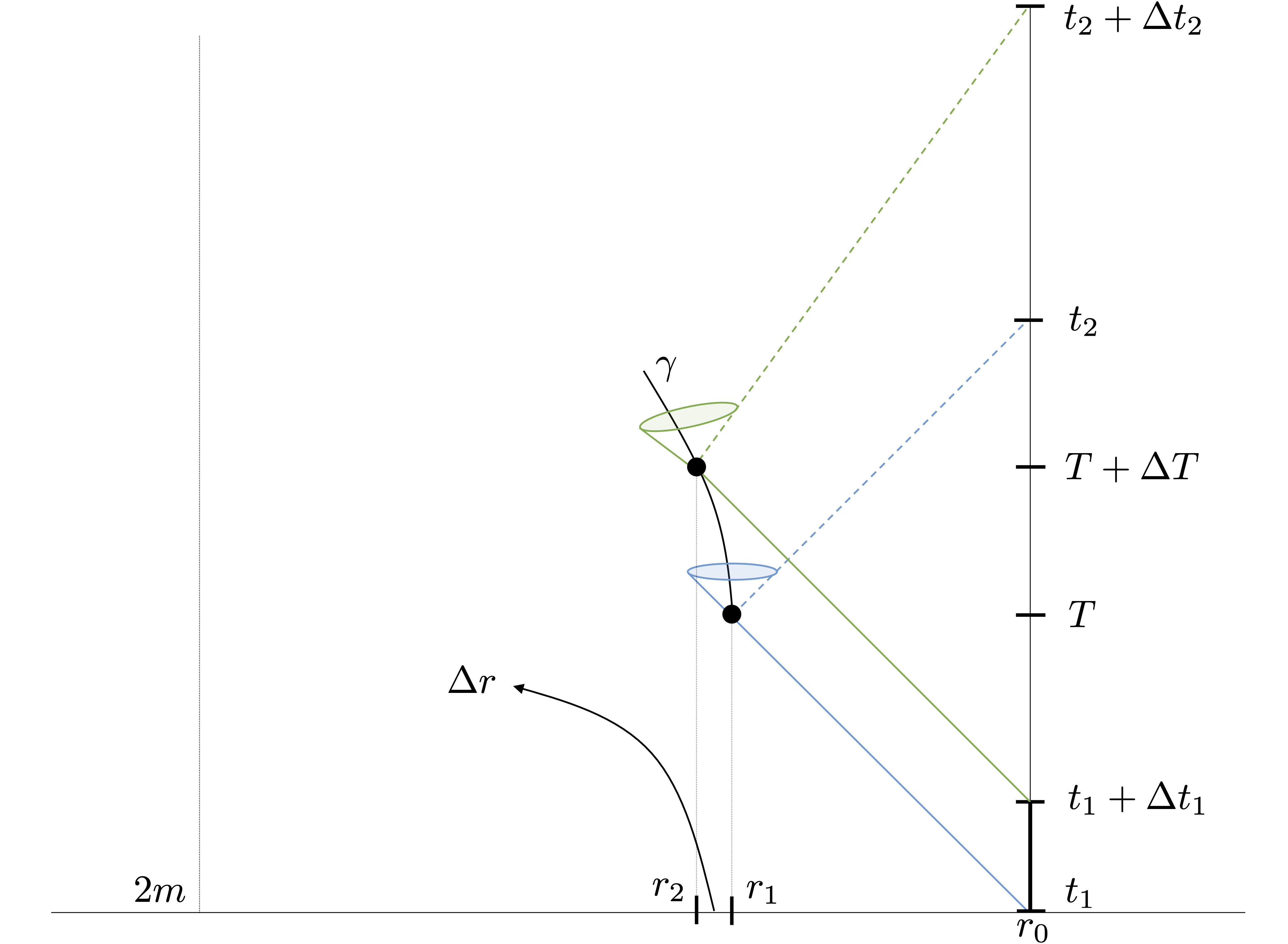
Figure 3: Sketch of the two-way Doppler mirror tracking in a Schwarzschild spacetime for radial mirror motion.

V Spacetime Application

For the following applications, we focus on Earth to satellite redshift measurement schemes to briefly illustrate the results above.

In axisymmetric and stationary spacetimes, we may choose coordinates $t,\varphi$ related to the symmetry, such that $\partial_{\varphi}$ is the spacelike Killing vector field of which the orbits are closed circles and $\partial_{t}$ is the Killing vector field related to time translations. The remaining two coordinates are labeled by $(x^{1},x^{2})$. We may write the metric as

$$g=-c^{2}e^{2\phi}\mathrm{d}t^{2}+2g_{t\varphi}\mathrm{d}t\mathrm{d}\varphi+g_{AB}\mathrm{d}x^{A}\mathrm{d}x^{B}+g_{\varphi\varphi}\mathrm{d}\varphi^{2}\,,$$ (90)

where $A,B=1,2$. There are constants of motion along a light ray and along the worldline of a geodesic observer, respectively,

$$(k_{t},k_{\varphi})\,,\quad(E:=-u_{t},L:=u_{\varphi})\,.$$ (91)

The remaining free functions are $u^{1},u^{2}$ and $k_{1},k_{2}$, which need to be determined from the geodesic equations for light and massive particles, respectively. The latter two are related to two emission angles, under which the light ray is sent to the receiver, i.e., the initial direction.

V.1 Schwarzschild spacetime

The metric in the usual coordinates is

$$g=-\left(1-\frac{2m}{r}\right)c^{2}dt^{2}+\left(1-\frac{2m}{r}\right)^{-1}dr^{2}\\ +r^{2}(d\vartheta^{2}+\sin^{2}\vartheta d\varphi^{2})\,.$$ (92)

We proceed to isotropic (harmonic) coordinates, which are better suited and allow for a straightforward post-Newtonian limit in the weak field approximation. In these coordinates, the metric reads

$$g=-\left(\dfrac{1-\rho_{s}/\rho}{1+\rho_{s}/\rho}\right)^{2}c^{2}dt^{2}\\ +\left(1+\rho_{s}/\rho\right)^{4}\left(d\rho^{2}+\rho^{2}(d\vartheta^{2}+\sin^{2}\vartheta d\varphi^{2})\right)\,.$$ (93)

Here, $\rho\in(\rho_{s},\infty]$ is the isotropic radial coordinate and $2\rho_{s}=m=GM/c^{2}$ and $m$ is the only non-vanishing mass moment, the monopole $\mathcal{M}_{0}$, in natural units. An observer on the Earth’s surface is located at some $\rho=\rho_{0}$ and the static redshift potential is

$$e^{\phi}=\left(\dfrac{2-m/\rho}{2+m/\rho}\right)\,.$$ (94)

Level surfaces are topological spheres $\rho=\text{const.}$ The redshift of two static observers becomes

$$z+1=e^{\Delta\phi}=\dfrac{(2-m/\rho_{0})(2+m/\rho)}{(2+m/\rho_{0})(2-m/\rho)}\,.$$ (95)

This expression allows to extract the weak-field limit as the contribution which is linear in $m$,

$$z=\Delta U/c^{2}\,,\quad U:=-\dfrac{GM}{R}\,,$$ (96)

where $R$ is the Euclidean radius. Note that the first part of the result above generalizes also to more complicated Newtonian gravitational potentials in the post-Newtonian formalism such that, to first order, the redshift is proportional to gravitational potential differences.

The Earth is rotating and, thus, there are Doppler contributions to the observed redshift. An observer on the rotating Earth has a four-velocity

$$(\tilde{u}^{\mu})=\tilde{u}^{t}(1,0,0,\tilde{v}^{\phi})\,,\quad\tilde{v}^{\phi}=:\tilde{\Omega}=\text{const.}$$ (97)

and a (geodesic or non-geodesic) satellite is described by

$$(u^{\mu})=u^{t}(1,v^{i})\,.$$ (98)

Their redshift is

$$1+z(t)=e^{\Delta\phi}\dfrac{\sqrt{1-e^{-2\phi_{0}}\dfrac{\tilde{v}^{2}}{c^{2}}}}{\sqrt{1-e^{-2\phi}\dfrac{v(t)^{2}}{c^{2}}}}\dfrac{1+\frac{k_{i}(0)v^{i}(t)}{k_{t}}}{1+b\tilde{\Omega}}\,,$$ (99)

with the constant impact parameter $b=k_{\varphi}/k_{t}$, and

$$\tilde{v}^{2} =\tilde{\Omega}^{2}\rho_{0}^{2}\left(1+\rho_{s}/\rho_{0}\right)^{4}\sin^{2}\vartheta_{0}\,,\quad\phi_{0}=\phi(\rho_{0})=\text{const.}$$

$$v^{2} =g_{ij}v^{i}v^{j}\,.$$ (100)

Introducing the new time scale $T=\exp(-\phi_{0})t$, which is the proper time of static clocks at $\rho_{0}$ (on the non-rotating geoid), the redshift becomes

$$1+z(T)=e^{\Delta\phi}\dfrac{\sqrt{1-\dfrac{\tilde{V}^{2}}{c^{2}}}}{\sqrt{1-e^{-2\Delta\phi}\dfrac{V(T)^{2}}{c^{2}}}}\dfrac{1+\frac{k_{i}(0)V^{i}(T)}{k_{T}}}{1+b\tilde{\Omega}}\,,$$ (101)

where $V^{i}=\exp(-\phi_{0})v^{i}$ is the observed velocity on the new time scale. If the satellite moves on a geodesic, we have

$$1+z(T)=e^{2\Delta\phi}\dfrac{E_{T}}{c^{2}}\dfrac{\sqrt{1-\dfrac{\tilde{V}^{2}}{c^{2}}}}{1+b\tilde{\Omega}}\left(1+\dfrac{k_{i}(0)V^{i}(T)}{k_{T}}\right)\,.$$ (102)

This relation can be used to create redshift models for geodetic satellites in the simple Schwarzschild spacetime. Note that the EOP needs to be solved for the unknown components of $k_{i}$

In general, the mass monopole can be determined from redshift measurements either between two Earth-bound observers or via Earth-satellite observations. In a very simple model, the satellite may move on a circular geodesic in the equatorial plane, leading to

$$z(b)=e^{2\Delta\phi}\dfrac{E_{T}}{c^{2}}\sqrt{1-\dfrac{\tilde{V}^{2}}{c^{2}}}\dfrac{\big{(}1+b\Omega\big{)}}{\big{(}1+b\tilde{\Omega}\big{)}}-1\,.$$ (103)

Note that the $b$ is a function of the satellite’s position. It can be related to the emission angle $\alpha$ w.r.t. the radial direction by

$$b=\dfrac{\tan\alpha\,\rho\left(1+\dfrac{m}{2\rho}\right)^{3}}{c\sqrt{1+\tan^{2}\alpha}\left(1-\dfrac{m}{2\rho}\right)}\,.$$ (104)

Hence, the redshift is a function of $\alpha$. Which angle $\alpha$ belongs to the momentary satellite position is to be determined by the solution to the EOP.

In a second simple model, we might use radial signal transfer such that $(k_{\mu})=(k_{T},k_{\rho},0,0)$ but do not require circular motion. Then

$$1+z(T)=e^{2\Delta\phi}\dfrac{E_{T}}{c^{2}}\sqrt{1-\dfrac{\tilde{V}^{2}}{c^{2}}}\left(1+\dfrac{k_{\rho}(0)V^{\rho}(T)}{k_{T}}\right)\,,$$ (105)

where

$$\dfrac{k_{\rho}(0)}{k_{t}}=\dfrac{\left(1+\dfrac{m}{2\rho}\right)^{3}}{\left(1-\dfrac{m}{2\rho}\right)}\,,$$ (106)

and $V^{\rho}$ is to be determined from the geodesic equation.

For the mirror tracking in Schwarzschild spacetime, we assume radial free-fall of the mirror to illustrate the idea. The result then is

$$1+z=\lim_{\Delta t_{1}\to 0}\dfrac{\Delta T}{\Delta t_{1}}=1+\dfrac{v}{c}\left(1+\dfrac{2GM}{c^{2}r}\right)+\mathcal{O}\left(c^{-4}\right)\,,$$ (107)

where $v$ is the line-of-sight velocity. Hence, observations of the two-way redshift allow to deduce the velocity as done in conventional Doppler tracking but contain also corrections due to the curvature (Shapiro delay).

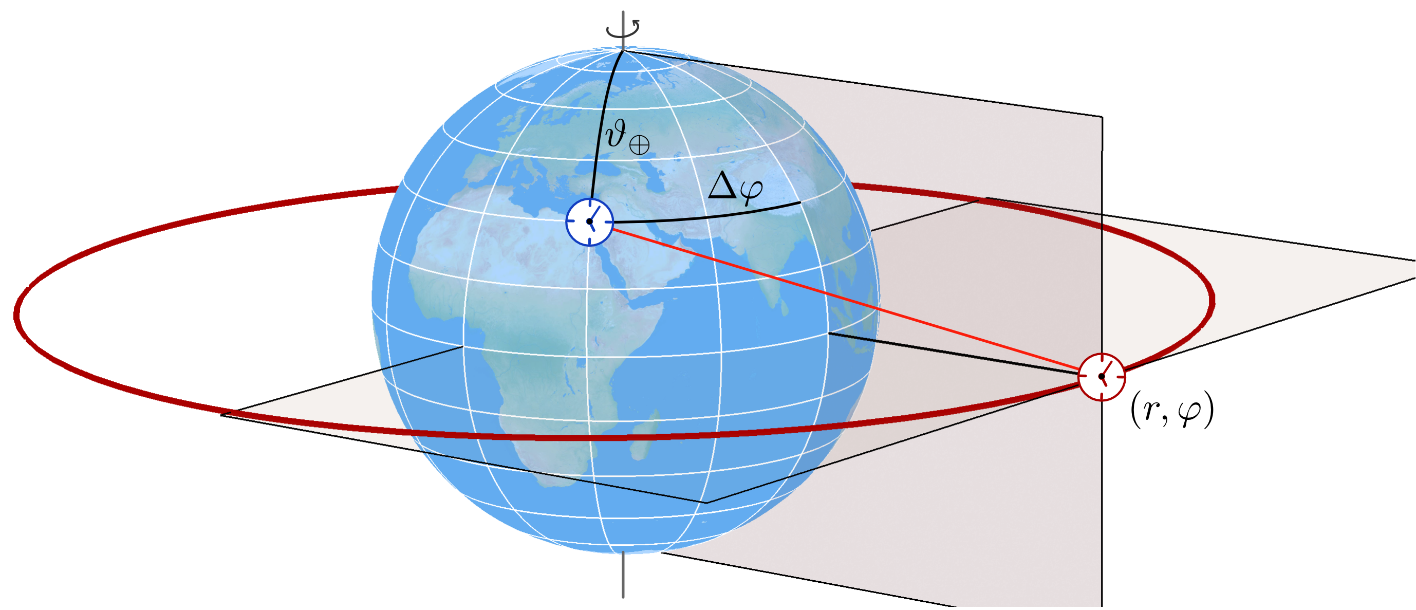
Figure 4: Sketch of signal exchange between an orbiting satellite and an Earth-bound clock.

V.2 Kerr

The Kerr metric in the well-known Boyer-Lindquist coordinates $(t,r,\vartheta,\varphi)$ reads

$$g =-\left(1-\dfrac{2mr}{\rho^{2}}\right)c^{2}dt^{2}+\dfrac{\rho^{2}}{\Delta}dr^{2}+\rho^{2}d\vartheta^{2}$$

$$+\sin^{2}\vartheta\left(r^{2}+a^{2}+\dfrac{2mra^{2}\sin^{2}\vartheta}{\rho^{2}}\right)d\varphi^{2}$$

$$-\dfrac{4mra\sin^{2}\vartheta}{\rho^{2}}\,c\,dtd\varphi\,,$$ (108)

where

$$\rho^{2}=r^{2}+a^{2}\cos^{2}\vartheta\,,\quad\Delta=r^{2}+a^{2}-2mr\,.$$ (109)

For the Kerr spacetime, the exists also a harmonic coordinate system, of which the non-rotation limit leads to the harmonic coordinates shown above. However, in these coordinates the metric functions become infinite series. Here, we introduce new coordinates $\varphi^{\prime}=\varphi-\omega t$, where $\omega$ is the angular velocity of an observer on the rotating Earth’s surface. Thus,

$$g_{tt}\to g_{tt}+\omega^{2}g_{\varphi\varphi}+2\omega g_{t\varphi}\,,\quad g_{t\varphi}\to g_{t\varphi}+2\omega g_{\varphi\varphi}\,.$$ (110)

In these coordinates, we have the redshift potential

$$e^{2\phi}=1-\dfrac{2mr}{\rho^{2}}+4\,\dfrac{\omega}{c}\,\dfrac{amr\sin^{2}\vartheta}{\big{(}r^{2}+a^{2}\cos^{2}\vartheta\big{)}}$$

$$-\,\dfrac{\omega^{2}}{c^{2}}\,\sin^{2}\vartheta\left(r^{2}+a^{2}+\dfrac{2mra^{2}\sin^{2}\vartheta}{r^{2}+a^{2}\cos^{2}\vartheta}\right)\,.$$ (111)

This redshift potential has two free parameters, $m$ and $a$. Let an observer on the Earth’s geoid Philipp et al. (2017, 2020) be at position $\tilde{x}=\tilde{x}_{0}=\text{const.}$ and make the proper time $T$ on the geoid a new coordinate time using ${T=\exp(-\phi(\tilde{x}))t=:\exp(-\phi_{0})t}$. The redshift w.r.t. any observer at position $x$ on the Earth’s surface is given by

$$z+1=e^{\phi_{0}-\phi(x)}\,.$$ (112)

Using the model of $\phi$, the two free parameters can be determined. If the second clock moves on an orbiting satellite, Eq. (71) can be used to determine the potential. If the satellite is on a geodesic, Eq. (72) can be used instead.

V.3 Higher-order multipoles

To study the effect of higher-order mass multipoles $\mathcal{M}_{i_{1}\dots i_{l}}$, we use a spacetime as defined by Thorne Thorne (1980) in an ACMC coordinate system $(t,x^{i})$ and the spin-dipole approximation.

$$g=-e^{2\phi}\left(cdt+\sigma_{i}dx^{i}\right)^{2}+e^{-2\phi}\gamma_{ij}dx^{i}dx^{j}\,,$$ (113)

where

$$\gamma_{ij}=e^{2\phi}(g_{ij}-\sigma_{i}\sigma_{j})\,,\quad g_{jk}=\delta_{jk}+\sum_{l=0}\dfrac{S_{l-1}}{r^{l+1}}\,,$$ (114)

and

$$\sigma_{i}=2e^{2\phi}\epsilon_{i3l}\mathcal{S}_{3}x^{l}\left(\dfrac{1}{r^{3}}+\dfrac{\mathcal{M}_{0}}{r^{4}}\right)\,,\quad S_{1}=0=S_{2}\,.$$ (115)

The direction of rotation is the $x^{3}$-axis and the spin dipole moment is given by $S_{3}$. For two geodesic observers we can use Eq. (57) to determine the multipole moments from measurements of the mutual redshift, the emission and reception direction of the exchanged light signal as well as satellites’ positions and velocities.

Eq. (46) can be used to model the Earth-satellite redshift. Again, the mass multipoles can be determined from fitting measurement data as outlined above.

Summary and Outlook

We have rigorously formulated the procedure of chronometric leveling from and in space. In doing so, we have provided a detailed analytical description of the methodology for determining the stationary (gravito-electric) gravitational potential while accounting for the motion of clocks. In pursuit of this goal, we devised a framework that combines the Doppler effect and gravitational redshift, enabling us to extract the gravitational potential. The same result can also be achieved using energy conservation along a satellite’s worldline. With the gravitational potential thus derived, we can proceed to calculate the mass multipole moments of the gravitational field from measurements, which in turn can be used to determine the geoid on Earth.

In the weak-field limit our results coincide with known notions and results. We emphasize that the entire approach is formulated within GR without approximation. This approach may evolve into a new data source for chronometry in space and relativistic geodesy in general, offering a chronometric approach to study the Earth’s gravity field in future missions.

The comparison of a ground based clock with a clock in space has a stability of at most $10^{-16}$. However, clock comparison between clocks on satellites does not suffer from atmospheric disturbances and may have a stability not worse than the clock stability. Further analysis is required to assess the precision of satellite speed measurements, a crucial factor for accurately accounting for Doppler shifts. To address this, we are currently developing a computer model that simulates a constellation of satellites equipped with precise clocks. This model will enable us to conduct comprehensive case studies to evaluate the overall accuracy in determining the gravitational potential. This is based on our existing High Precision Satellite modeling software package Philipp et al. (2018).

Appendix A On modeling the redshift

A useful approach to model the redshift between given emitter and receiver worldlines might be the following. Assume that the worldlines $\gamma$ and $\tilde{\gamma}$ are known. From an event $p\in\operatorname{img}(\gamma)$ (emission event) we send light signals $\lambda_{n}$ in all directions (a spherical wave), which are labeled by some index $n$. The set of spatial trajectories (orbits) of these light rays is denoted by

$$O(\lambda):=\bigcup\limits_{n}O(\lambda_{n})\,,\quad O(\lambda_{n}):=\{(x^{i}):(t,x^{i})\in\text{img}(\lambda_{n})\}\,,$$ (116)

and

$${O(\tilde{\gamma}):=\{(\tilde{x}^{i}):\tilde{p}=(\tilde{t},\tilde{x}^{i})\in\text{img}(\tilde{\gamma})\}}$$ (117)

is the orbit of the observer on $\tilde{\gamma}$.

All intersection points of $O(\lambda)$ with $O(\tilde{\gamma})$, i.e., $O(\tilde{\gamma})\cap O(\lambda)$ are calculated (numerically). For any element in $O(\tilde{\gamma})\cap O(\lambda)$, the velocity $\tilde{u}$ at that position can be calculated and the corresponding redshift follows (consider only a single orbit for uniqueness in case of bound motion). Of course, given the true worldline $\tilde{\gamma}$, the receiver of the signal is only at one of those intersections for any chosen emission event. Now, this procedure is repeated for every $p\in\text{img}(\gamma)$ to construct all possible redshift values as a function of emission time (coordinate time $t$ at $p$) and reception time $\tilde{t}$ (coordinate emission time + coordinate travel time). This defines a two-dimensional surface $z(t,\tilde{t})$ and the true, measured redshift is a one-dimensional subset – it is related to the projection of the image of the map $\bar{\Lambda}$ onto this surface. The open question here is if this true redshift can be geometrically characterized by a special curve on the surface. This method may be of interest as well when a (continuous) distribution of clocks is considered, e.g., on the rotating Earth and a satellite in orbit sends signals towards all of these clocks. Note the similarity to ray tracing approaches.