The JWST Early Release Science Program for Direct Observations of Exoplanetary Systems III:
Aperture Masking Interferometric Observations of the star HIP 65426 at $\boldsymbol{3.8\,\rm{\mu m}}$

Abstract

We present aperture masking interferometry (AMI) observations of the star HIP 65426 at $3.8\,\rm{\mu m}$ as a part of the JWST Direct Imaging Early Release Science (ERS) program obtained using the Near Infrared Imager and Slitless Spectrograph (NIRISS) instrument. This mode provides access to very small inner working angles (even separations slightly below the Michelson limit of ${}0.5\lambda/D$ for an interferometer), which are inaccessible with the classical inner working angles of the JWST coronagraphs. When combined with JWST’s unprecedented infrared sensitivity, this mode has the potential to probe a new portion of parameter space across a wide array of astronomical observations. Using this mode, we are able to achieve a contrast of $\Delta m_{F380M}{\sim}7.8$ mag relative to the host star at a separation of ${\sim}0.07\arcsec$ but detect no additional companions interior to the known companion HIP 65426 b. Our observations thus rule out companions more massive than $10{-}12\,\rm{M\textsubscript{Jup}}$ at separations ${\sim}10{-}20\,\rm{au}$ from HIP 65426, a region out of reach of ground or space-based coronagraphic imaging. These observations confirm that the AMI mode on JWST is sensitive to planetary mass companions orbiting at the water frost line, even for more distant stars at $\sim$100 pc. This result will allow the planning and successful execution of future observations to probe the inner regions of nearby stellar systems, opening essentially unexplored parameter space.

1 Introduction

JWST (Gardner et al., 2006, 2023) has established itself as the world’s pre-eminent infrared observatory. The Near-Infrared Imager and Slitless Spectrograph instrument (NIRISS, Doyon et al., 2012, 2023), is equipped with a sparse aperture mask (Sivaramakrishnan et al., 2009, 2023a). This mask enables the Aperture Masking Interferometry (AMI, Baldwin et al., 1986; Haniff et al., 1987; Readhead et al., 1988) mode on the telescope, which is available for the first time from space. This facilitates the execution of science cases that can use moderate contrast at small angular separations, for example, high-resolution imaging of extended sources, structure identification of Solar System objects (e.g. Jupiter’s moon Io) and imaging extremely bright objects like Wolf-Rayet stars.

A particularly powerful feature of this mode is its ability to directly image planetary mass companions (PMCs) inside the Rayleigh diffraction limit, ${\lesssim}\lambda/D$ (where $D$ is the aperture size of the telescope and $\lambda$ is the observing wavelength). With the JWST/NIRISS/AMI mode, contrasts of ${\sim}{10^{-3}}{-}{10^{-4}}$ are predicted to be achievable with sufficient integration times (Soulain et al., 2020; Rigby et al., 2022). This mode is well equipped to directly detect or place constraints on additional inner companions of systems with already-known wide-separation companions. Such systems have historically revealed the presence of additional companions at smaller orbital separations (Marois et al., 2010; Nowak et al., 2020; Hinkley et al., 2023), which has also been demonstrated by theoretical studies (Wagner et al., 2019). Using AMI to expand the parameter space inwards will hence enable the community to provide a more robust characterization of the orbital architectures of planetary systems. In addition to this, the mode is also predicted to access Jupiter mass companions at water frost-line separations around stars in nearby young moving groups/associations (Sallum et al., 2019; Ray et al., 2023). Going forward, this will be a promising technique for placing constraints on initial entropies (by using in conjunction, planetary mass estimates from e.g. Gaia) of planets for at least the next decade (Spiegel & Burrows, 2012; Ray et al., 2023).

The Director’s Discretionary Early Release Science (DD-ERS) Program 1386 (Hinkley et al., 2022) includes AMI observations to demonstrate the observing mode and test its feasibility for these science cases. In this paper we report the results of the AMI observations of the ERS program, of the star HIP 65426 (A2V, $109.20\pm 0.74\,\rm{pc}$), observed at $3.8\,\rm{\mu m}$. This star has a previously known companion HIP 65426 b (Chauvin et al., 2017; Cheetham et al., 2019), with a projected separation of $86^{+116}_{-31}\,\rm{au}$ and a mass of $7.1\pm 1.2\,\rm{M\textsubscript{Jup}}$ (Carter et al., 2023). In this paper we present the scientific results of the ERS 1386 AMI observations, placing new constraints on the presence of additional companions in the HIP 65426 system and demonstrating its potential for similar observations in other nearby systems. In an accompanying paper (Sallum et al., 2023) we analyze the performance, achievable contrast, and limiting noise sources of this mode.

This work was carried out in parallel with other science aspects of the ERS program. These included (1) coronagraphic observations of HIP 65426 b at $2{-}5\,\rm{\mu m}$ with the Near-Infrared Camera (NIRCam) and $11{-}16\,\rm{\mu m}$ with the Mid-Infrared Instrument (MIRI) (Carter et al., 2023), (2) the highest fidelity spectrum to date of a planetary-mass object, VHS 1256 b (Miles et al., 2023) and, (3) coronagraphy out to 15.5 $\mu$m of HD 141569A, a young circumstellar disk, with particular focus on sampling the disk brightness on and off the $3.0\,\mu m$ H₂O ice feature (Millar-Blanchaer et al. in prep, Choquet et al. in prep).

In §2 we give a brief summary of the AMI mode with JWST, followed by our observation strategy in §3. In §4 we detail the various data processing steps. In §5 we summarise our discussion and in §6 we present the principal conclusions of this study.

2 JWST Aperture Masking Interferometry

AMI transforms a conventional telescope into an interferometric array via a pupil-plane mask (Tuthill et al., 2001). This is typically accomplished using a piece of metal with holes (sub-apertures) cut out of it. The images recorded by the detector are then the interference fringes produced from the light after passing through the sub-apertures, which can be analysed using Fourier techniques. When each baseline in an aperture mask has a unique position angle and separation, a linear relationship between pupil-plane phase differences and measured fringe phase exists. Due to this non-redundancy, Fourier observables (e.g. closure phases, squared visibilities, see §4.2) can be calculated which are robust to first-order residual phase errors (following the description in Ireland, 2013).

This technique has been successfully carried out using ground based facilities (e.g. Tuthill et al., 2000; Monnier et al., 2007; Kraus & Ireland, 2012; Hinkley et al., 2015) and is for the first time being executed in space with JWST (Sivaramakrishnan et al., 2023b; Kammerer et al., 2023). This is achieved using a mask with seven hexagonal sub-apertures (see Figure 1), each of which has an incircle diameter of $0.8\,\rm{m}$, when projected onto the JWST primary mirror (Sivaramakrishnan et al., 2012; Greenbaum et al., 2015). This probes $\left({}^{7}_{2}\right)$, or 21 distinct spatial frequencies (number of baselines) and $\left({}^{7}_{3}\right)$, or 35 closure phase triangles. This mode can be used with four NIRISS filters at wavelengths $2.77\,\rm{\mu m}$ (F277W), $3.80\,\rm{\mu m}$ (F380M), $4.30\,\rm{\mu m}$ (F430M), and $4.80\,\rm{\mu m}$ (F480M). These wavelength channels are specifically designed to be sensitive to H₂O, CH₄, CO₂ and CO features respectively (e.g. Figure 1 of Soulain et al., 2020).

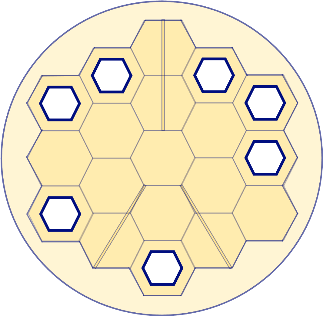
Figure 1: Schematic diagram of the non-redundant mask onboard JWST/NIRISS containing seven sub-apertures.

3 Observing Strategy

The AMI observations were performed using the F380M filter and the SUB80 subarray with the NISRAPID readout pattern. The F380M filter was specifically chosen from the available filters to reach smaller angular separations than the F430M and F480M filters, to detect close-in companions whilst making sure the central wavelength was close to the region of the spectrum where exoplanets are the brightest (at ${\sim}4{-}5\,\rm{\mu m}$, e.g. Figure 2 of Ray et al., 2023, as compared to F277W filter which spans wavelengths where exoplanets are relatively faint).

The observing setup was designed such that a photon noise limited observation would be able to access a contrast of $\Delta_{mag}{\sim}10$ (Ireland, 2013). The appropriate number of groups and integrations were hence chosen to collect $\sim 10^{10}$ photons for each target while avoiding saturation or non-linearity effects (Table 1). All the observations were carried out following the recommended best practices as known prior to launch and described in the JWST user documentation.

To ensure optimal data analysis of the AMI observations, point spread function (PSF) reference stars are required to be observed, in addition to the science target. This is executed because while Fourier observables are robust to phase errors to first order, higher order errors remain that must be calibrated out (Ireland, 2013). These reference stars should be point sources so that they measure only the instrumental contributions to the errors in the observables, which in turn, ensures the optimal calibration of the target star observations. The target star was planned to be observed with the most time and the calibrators were chosen to be relatively bright stars, close to the target star on the sky plane. This would ensure that we obtained similar number of photons from the calibrators as the target star, with shorter exposure times (see Table 1). However, for future observations with this mode, calibrators with similar brightness as the target star should be chosen, as the detector systematics are the limiting factor in terms of reaching the required contrast for datasets of this depth (see §4.2 and Sallum et al. (2023) for more details).

For the AMI sequence of this program, the observation of the target star HIP 65426 was preceded by one calibrator (HD 115842) and followed by another calibrator (HIP 65427) (see section 3.1 for details). Observations of two calibrator stars reduces the risk of encountering calibrators with unexpected resolved structure (e.g. close-in companions, disks). Observing the target star in the middle of the sequence between two calibrator stars which are close on the sky plane (1) is advantageous towards reducing the wavefront drift and, (2) ensures that the time elapsed during the slew between the target and the reference stars is kept to a minimum, which minimises thermal drifts by pointing changes. This ensures that the changing spacecraft attitude does not cause a change in the temperature of the primary mirror segments and subsequently affect the Fourier phases observed by the telescope. The PSF reference stars are then used to calibrate out instrumental contributions to the interferometric observables (see §4). An example raw image taken with the JWST/NIRISS/AMI mode of the science target (HIP 65426) is shown in the left panel of Figure 2.

3.1 Vetting of the calibrator stars

To ensure the calibrator stars, HD 115842 and HD 116084, were point sources, they were vetted first using Search Cal (Bonneau et al., 2006), and were then followed up with observations using ground based facilities. This was firstly done with the speckle imaging observations from Southern Astrophysical Research (SOAR) telescope’s High Resolution Camera (HRCam, Tokovinin et al., 2010) instrument. Both calibrators (HD 115842 and HD 116084) were found to be unresolved point sources. In addition to this, these stars were checked for binarity with AMI observations with the VLT/SPHERE/IRDIS (Cheetham et al., 2016) integral field spectrograph (Proposal ID: 109.24EY). Both stars were found to be unresolved point sources, with an average contrast limit of $\Delta_{mag}{\sim}6$, calculated across the 39 IRDIS wavelength bins. This contrast was achieved at separations of ${\sim}\lambda/D$ for both stars, which corresponds to separations of $23{-}40\,\rm{mas}$ given the IRDIS wavelength range of $0.95{-}1.60\,\rm{\mu m}$.

Table 1: Parameters for the NIRISS/AMI observations in the F380M filter. The observations were executed on 30 July 2022 (UTC). The start and the end times indicate the start and the end of the observation block at UTC and are not directly related to the exposure times. The target star, HIP 65426 was observed between the calibrator stars HD 115842 and HD 116084.

Star	Type	Start time	End time	Sequence	Readout	Ngroups	Nints	Dithers	texp (s)
HD 115842	Calibrator	05:26:46	06:52:10	1a	NISRAPID	2	10000	1	2468.00
				1b	NISRAPID	2	5500	1	1357.40
HIP 65426	Target	07:02:39	10:53:00	2a	NISRAPID	13	10000	1	10766.40
				2b	NISRAPID	13	950	1	1022.81
HD 116084	Calibrator	11:02:17	12:49:58	3a	NISRAPID	3	10000	1	3222.4
				3b	NISRAPID	3	6000	1	1933.44

4 Data Reduction and Extraction of Fourier Observables

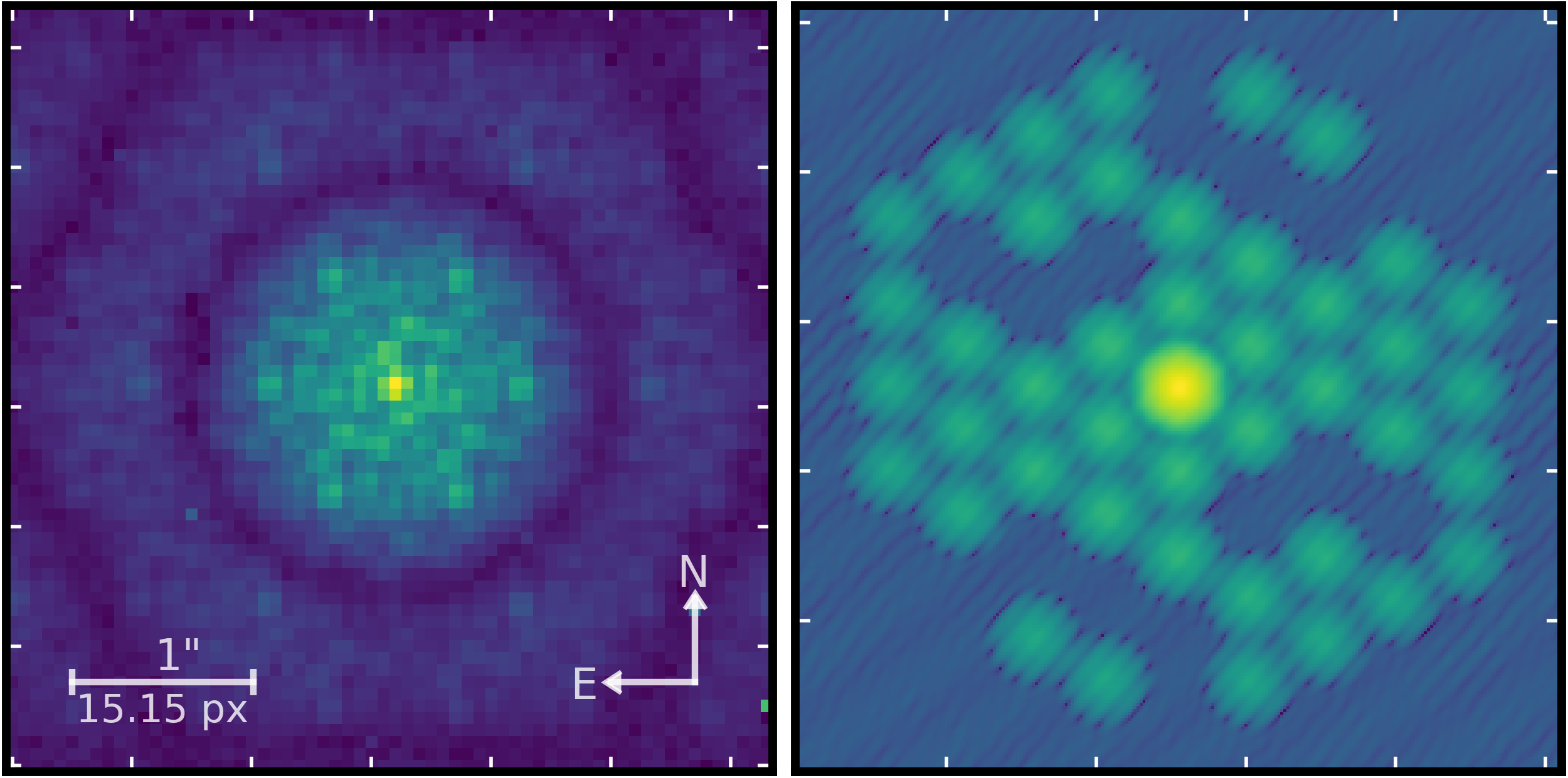
Figure 2: On the left is the science raw image of the observation. This pattern (interferogram) is obtained on the detector and is a result of the interference of the light emerging from each of the sub-apertures of the mask as shown in Figure 1. On the right is the associated power spectrum of the science image which is essentially its Fourier transform. The power spectrum is used to extract the orbital properties of a potential companion in the star system by analysing the Fourier observables. The observations in the figure are taken at $3.80\,\rm{\mu m}$.

.

As part of the science enabling products produced by this ERS team, we have developed SAMpy (Sallum et al., 2022), which primarily handled the processing of this dataset, in conjunction with the jwst (Bushouse et al., 2022) pipeline. SAMpy is a publicly available python package containing data reduction tools tailored for JWST/NIRISS/AMI, and is flexible enough to adapt to arbitrary masking setups (e.g. VLT/SPHERE, LBT/LMIRCam, Keck/NIRC2). It processes the AMI data using a Fourier-plane approach. The accompanying paper Sallum et al. (2023) covers a detailed description and justification of the processing steps undertaken for this dataset, which is briefly outlined in the following sections for clarity.

4.1 Pre-processing of the data

To prepare the data for the calculation of the Fourier observables, some pre-processing steps using SAMpy were executed. The first step in this process was to identify and correct bad pixels. First, the bad pixel map was produced by the jwst stage 1 pipeline, which flags all “DO NOT USE” pixels in the Data Quality (DQ) array as bad. This was followed by identifying additional bad pixels using the statistics of the individual integrations and the set of integrations. All such bad pixels were corrected, using the Fourier-plane approach taken in Kammerer et al. (2019). Finally, each image was centred to pixel-level precision, cropping to a smaller size of $64{\times}64$ pixels, before applying a 4th-order super-Gaussian window with a FWHM of 48 pixels. This process is described in detail in Sallum et al. (2023).

4.2 Data processing and model fitting

Once the processed image was obtained, the Fourier observables were calculated from the Fourier transform of the image (the power spectrum is shown in the right panel of Figure 2). First, the complex visibilities were calculated which comprise the amplitudes and phases associated with the unique mask baselines. This was followed by the calculation of squared visibilities, which are the powers (amplitudes squared) associated with each of the unique mask baselines. Next, the closure phases were computed, which are the sums of phases for baselines forming a triangle.

After the calculation of the above, the observations were calibrated. Calibrating the observations for the science target (HIP 65426) was explored by calibrating it separately with each of the calibrator stars HD 115842 and HD 116084 respectively, in addition to calibrating it with both the calibrator stars together. It was found that using HD 116084 solely to calibrate the science target yielded the best results in terms of reaching the deepest contrast ($\Delta m_{F380M}{\sim}7.8$, see third column of the top panel of Figure 3). The two likely reasons for this are that this observation had more similar charge migration properties to HIP 65426, and used a larger number of groups (three, as opposed to two for HD 115852). Both of these characteristics result in better minimization of PSF artefacts and detector systematics during data reduction and subsequent AMI calibration, making for a better calibrated dataset (Sallum et al., 2023). Hence, only HD 116084 was used for the calibration for the analysis in this paper.

The calibration was done by (1) dividing the squared visibilities of the target by those of the calibrator and, (2) subtracting the closure phases of the calibrator from the target closure phases (see Figure 3). As described in Sallum et al. (2023), we calculate both statistical error bars and systematic error bars for the closure phases and squared visibilities. We calculate statistical error bars by measuring the standard deviation of each quantity across all integrations. However, these are significantly smaller than the residual calibration errors in the data. We thus also estimate systematic error bars by measuring the standard deviation of the closure phases and squared visibilities across the triangles and baselines, respectively.

4.3 Companion Model Fitting

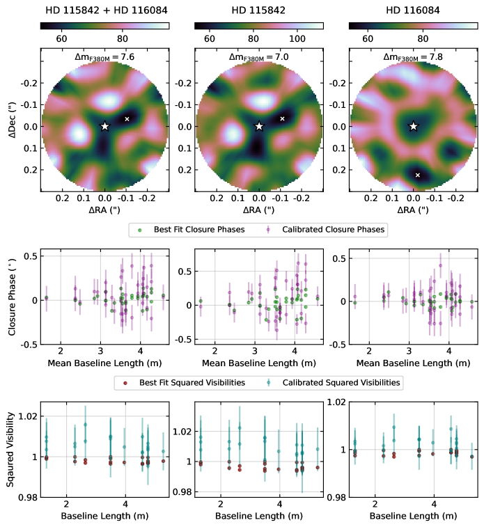
Figure 3: The first column shows the HIP 65426 data calibrated with both calibrators (HD 115842 and HD 116084), the second column shows the data calibrated with only HD 115842, and the third column shows the data calibrated with only HD 116084. The first row shows the $\chi^{2}$ surfaces in right ascension and declination, at the best-fit companion contrast for each the HIP 65426 calibration. The second and third rows show the corresponding best fit Fourier observables of closure phases and squared visibilities respectively, compared to the data. The ‘$\filledstar$’ symbols in the $\chi^{2}$ maps in the first row show the position of the central star and the ‘$\times$’ symbols show the best fit companion positions for each calibration. The best fit $\Delta{m_{F380M}}$ contrast value for each calibration is also displayed in the panels of the first row. As discussed in Section 4.3, we conclude that no companions are detected based on: (1) the inconsistent companion solutions from calibration to calibration, (2) the lack of a single clearly-defined region of low $\chi^{2}$ value for individual calibrations, and (3) the similarity in these fit results to those for simulated noise (see Figure 4).

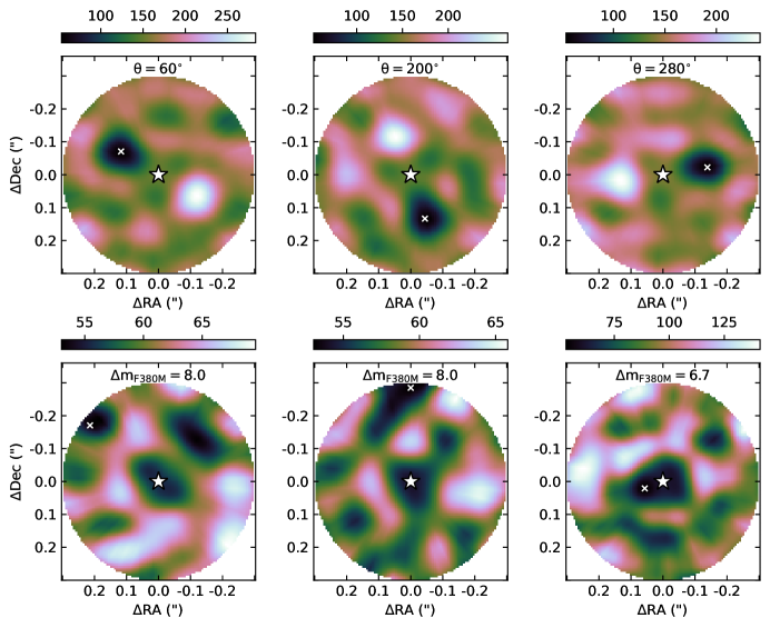
Figure 4: The top row shows the $\chi^{2}$ maps of datasets calibrated with HD 116084 (see third column of first row of Figure 3) with injected companions of $\Delta{m}_{F380M}=6.0$ at different positions angles ($\theta$, measured anti-clockwise from the vertical axis). Similar to Figure 3, the ‘$\filledstar$’ symbols in the $\chi^{2}$ maps show the position of the central star and the ‘$\times$’ symbols show the best fit companion positions. These injected companions are detected with high significance, as shown by the clearly-defined regions of low $\chi^{2}$ values at the injected position angles in each plot. The bottom row shows the $\chi^{2}$ maps for three Gaussian noise simulations, with the same standard deviation as that measured for the calibrated HIP 65426 dataset. At the top of these plots in the bottom panel, is the best fit $\Delta m_{F380M}$ contrast value. These contrast values overlap with the best-fit contrasts for the HIP 65426 companion fit, and the $\chi^{2}$ surfaces display the same lack of a single, clearly-defined minimum. Together these factors demonstrate that the fit results for HIP 65426 can be caused by noise alone.

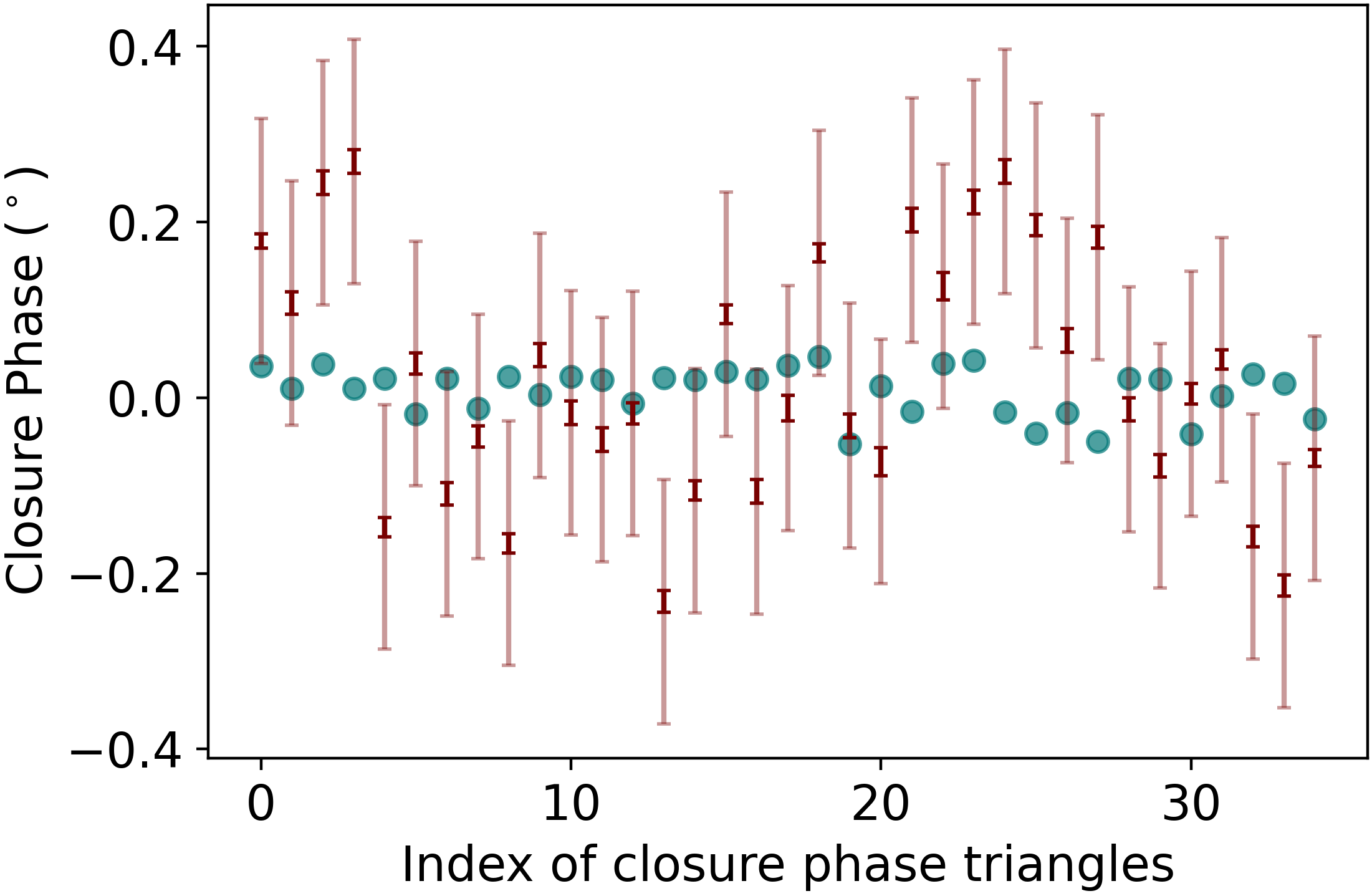
Figure 5: The expected closure phase signal from the known planet HIP 65426 b is shown with cyan circles and the maroon lines are the measured closure phases from the observation.

We fit companion models to Fourier observables via both grid and Markov-Chain Monte Carlo (MCMC) methods (utilising the emcee Python package, Foreman-Mackey et al., 2013). The analytic models consist of a delta function central point source (representing the star) and an ensemble of delta function companions each with a separation, position angle, and contrast relative to the central star, individually selected such that a binary model (containing the central star and one companion) most closely resembles the calculated Fourier observables. The grid output was used to generate the $\chi^{2}$ surface for positional parameters at the best-fit companion contrast as shown in the top panel of Figure 3 (with each panel showing a different calibration).

While a best-fit model can be found for each dataset, the best-fit models differ from one calibration to another, with contrasts between $\Delta m_{F380M}=7.0-7.8$ and widely varying separations and position angles. Furthermore, in all three calibrations, a single clearly defined region of low $\chi^{2}$ value does not exist. It should be noted that the method for estimating systematic error bars (measuring the standard deviation of the time-averaged closure phases and squared visibilities) causes the reduced $\chi^{2}$ values of the best fits in Figure 3 to be close to one. This does not necessarily represent the quality of the fit, but rather the large systematic uncertainties in the calibrated data. Thus, the inconsistent solutions from calibration to calibration and the lack of a clearly-defined single $\chi^{2}$ minimum in any individual calibration argue against additional companions in this dataset.

Here we use noise and companion injection simulations to explore this further, specifically for the HD 116084 calibration since it yielded the lowest scatter and thus achievable contrast. We first performed fits to Gaussian noise with the same standard deviation as the closure phases and squared visibilities for the HIP 65426 data calibrated with HD 116084. The bottom panel of Figure 4 shows the resulting $\chi^{2}$ maps at the best-fit companion contrast for three noise realisations. The best-fit contrasts, which range from $\Delta m_{F380M}=6.7-8.0$ overlap with the $\Delta m_{F380M}=7.8$ mag result for HIP 65426. This shows that the companion fit result shown in the right column of Figure 3 can be caused by noise alone.

For comparison, in the top panel of Figure 4, we show $\chi^{2}$ maps of the calibrated (with HD 116084) data (HIP 65426) with injected companions of $\Delta m_{F380M}=6.0$ at different position angles ($\theta=60^{\circ}$, $\theta=200^{\circ}$ and $\theta=280^{\circ}$ respectively). The injected companions are clearly detected as distinct regions of low $\chi^{2}$ values with preferred positions, unlike the noise realisations and the calibrated data (in Figure 3). Increasing the companion contrast to levels of $\Delta m_{F380M}=7-8$ magnitudes eventually causes the resulting $\chi^{2}$ surfaces to become indistinguishable from noise. This is one measure of the achievable contrast of these data, which we further discuss in Section 4.4.

Lastly, we compare the HIP 65426 data calibrated with HD 116084 to expectations for the signal from the known companion in the system, HIP 65426 b (Chauvin et al., 2017; Carter et al., 2023). Figure 5 shows the results. The expected closure phase signal from HIP 65426 b is shown with cyan circles. The calculated closure phase signal from the observation is shown in maroon with error bars. The smaller error bars are the statistical errors calculated from the science and calibrator observations added in quadrature. The longer error bars are the standard deviation of the calibrated closure phases of the science target (the difference between the science and the calibrator observations, see §4.2). Figure 5 shows that the signal from HIP 65426 b is significantly lower level than the scatter in the calibrated data, making the known companion undetectable. This is largely due to the fact that the spatial frequency coverage of NIRISS AMI mask would alias signals with separations as wide as HIP 65426 b.

4.4 Accessible Companion Contrast

A contrast curve was generated from a single-companion fit model. This was executed following an approach similar to Sallum et al. (2019), which is briefly discussed here for clarity (see also Sallum et al. (2023)). The calibrated closure phases and squared visibilities were compared to a grid of single companion models with different separations, contrasts, and position angles. For each companion separation, the average $\chi^{2}$ value of all the sampled position angles ($\chi^{2}_{sep}$) was calculated. Finally, the $5\sigma$ contrast was taken to be the contrast at which $\Delta\chi^{2}=\chi^{2}_{sep}-\chi^{2}_{null}=25$, where $\chi^{2}_{null}$ is the $\chi^{2}$ calculated for the null (no companion) model. The $\Delta\chi^{2}$ value of 25 is taken since one parameter (contrast) determines the difference between the null model and the 5$\sigma$ detectable model at each separation. This 5$\sigma$ curve is shown in Figure 6 in dark purple. Since phase is sensitive to asymmetry, at close-in separations less sensitivity is achieved for companions with equal brightness. This is the reason at separations ${\lesssim}0.05\,\arcsec$, the contrast curve shows a degeneracy. The figure also shows the simulated contrast curve of the observation from Hinkley et al. (2022) in light purple.

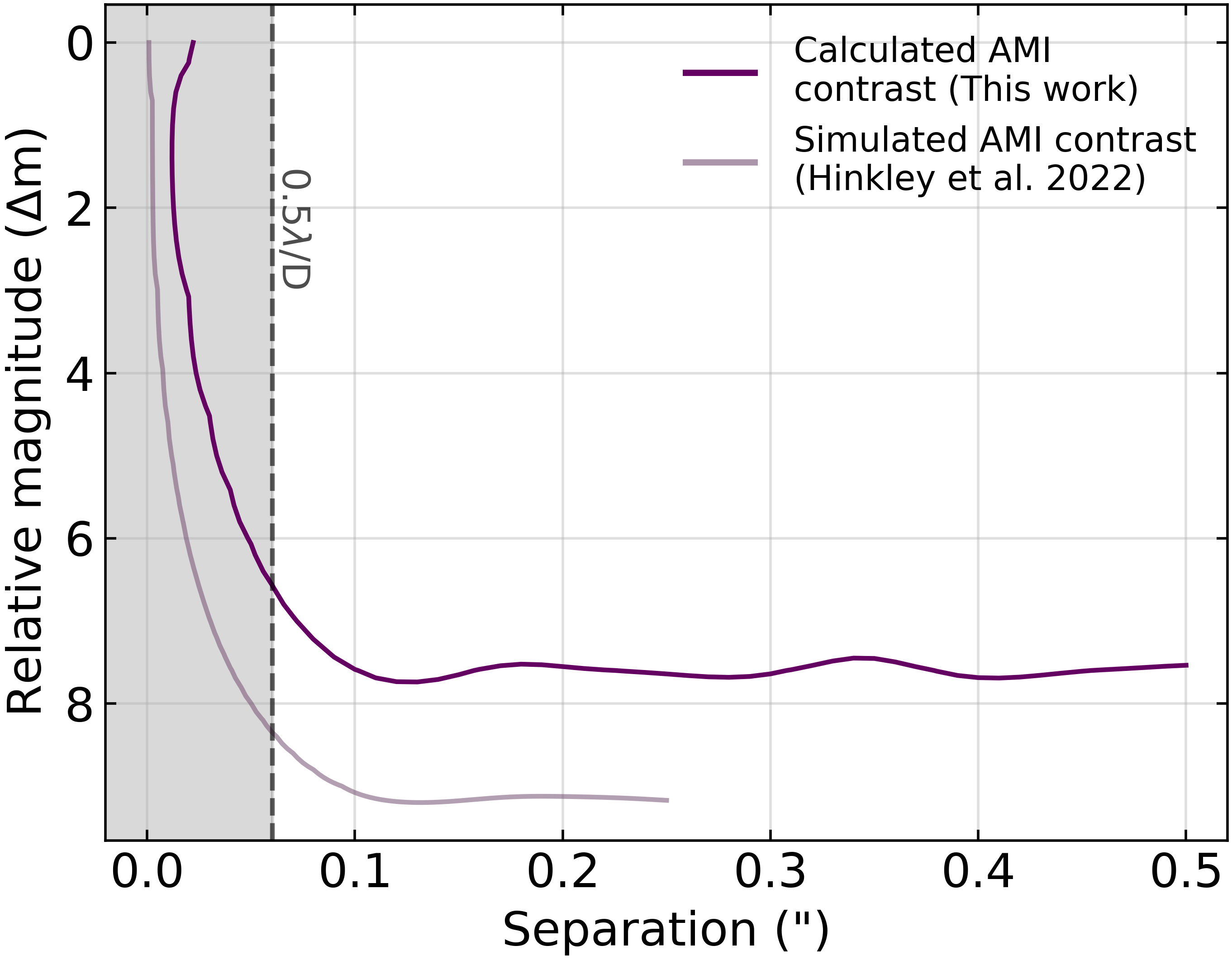
Figure 6: The calculated $5\sigma$ contrast curve for our observation is shown in purple, which was obtained using closure phases. The analogous simulated observation is shown in light purple, which was optimistic by ${\sim}1{-}2$ mag. The inner working angle for AMI observations is essentially $0.5\lambda$/D (Michelson diffraction limit). Separations below this limit are therefore greyed out.

5 Discussion

As evident from Figure 6, the contrast curve from actual data (this work) underperforms compared to the simulated contrast curve of the observation (Hinkley et al., 2022). Below we briefly discuss possible reasons for this discrepancy, which are explored in quantitative detail in the companion paper Sallum et al. (2023). We also discuss how the accessible contrast in magnitudes translates to the accessible mass limits based on different evolutionary models.

5.1 Discrepancy with Simulations

As discussed in detail in Sallum et al. (2023), the discrepancy between the simulated and observed contrast curves most likely arises from the fact that the contrast is limited by the effect of charge migration (the brighter-fatter effect, Hirata & Choi, 2020), rather than being limited by the photon noise limit. The charge migration effect is exhibited by infrared detectors when the electric field induced by accumulated charges deflects new charges. This causes two nearby pixels to accumulate charge at different rates, with the brighter pixel apparently spilling photoelectrons into its neighbouring pixels. For brighter objects, this results in a FWHM of the PSF with larger spatial extent.

In addition to masking the presence of fainter companions in the close vicinity of a bright star, charge migration can cause brightness-dependent PSF differences (and thus calibration errors) between a science target and reference PSF target. This effect was not taken into account during the generation of the simulated contrast curve shown in Figure 6. If we had the same level of charge migration between science and calibrator observations, we would have improved contrast quality and would have reached closer to the simulated achievable contrast (Sallum et al., 2023). To plan observations with this mode in future cycles, observations should ideally target PSF references that well-matched to the science target in brightness.

5.2 Mass Sensitivity Limits

To compute the mass sensitivity accessible with the calculated contrast curve, multiple evolutionary models were used (see Figure 7). An age value of $14\,\rm{Myr}$ (as discussed in Appendix A of Chauvin et al., 2017) was used for the analysis across all used models.

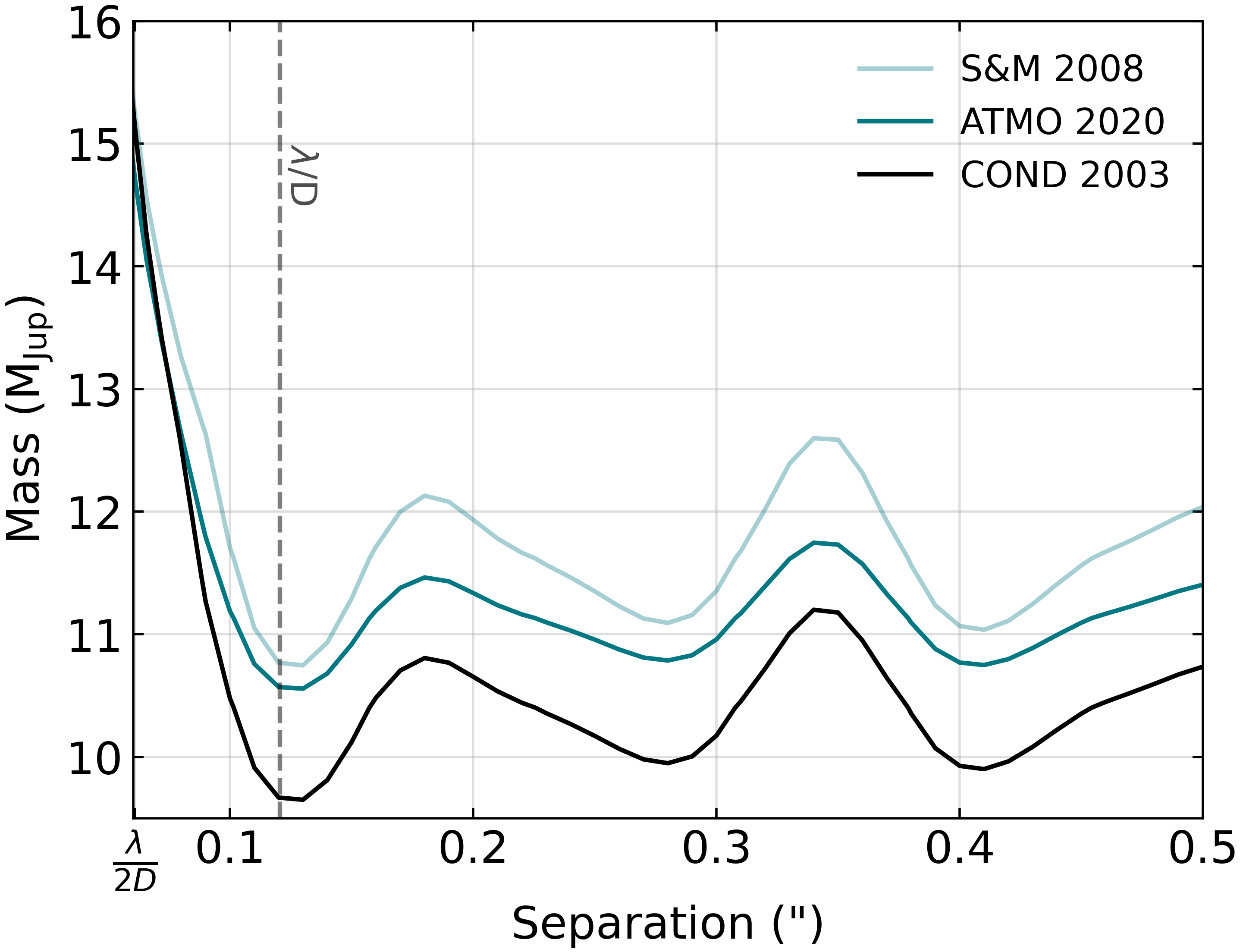
Figure 7: The accessible mass limits using the contrast curve from Figure 6 is shown in this Figure. The light cyan curve utilises the cloudy models from Saumon & Marley (2008), the dark cyan curve utilises the equilibrium case of ATMO 2020 (Phillips et al., 2020) and the black curve employs COND 2003 (Baraffe et al., 2003). The lower limit on the x-axis is ${\sim}0.5\lambda/D$, which is approximately the practically achievable inner working angle with AMI. The dashed grey line shows the conventional diffraction limit below which the contrast curve begins to grow steeply for accessible mass limits.

5.2.1 ATMO 2020 Atmosphere Models

The mass detection limits were calculated from the generated contrast curve using the ATMO 2020 (Phillips et al., 2020) set of models, similar to the method in Ray et al. (2023). ATMO 2020 is a set of radiative-convective one-dimensional equilibrium cloudless models describing the atmosphere and evolution of cool brown dwarfs and self-luminous giant exoplanets, spanning the mass range of ${\sim}0.5{-}75\,\rm{M\textsubscript{Jup}}$. Even though these models are cloudless, they mimic the effect of clouds by using a lower temperature profile. The model is computed in three different sets of evolutionary models: one at chemical equilibrium, and two at chemical disequilibrium assuming vertical mixing at different strengths. We keep our calculations and results limited to the case of equilibrium models, since this case provides the baseline scenario of planetary atmospheric conditions, and does not take into account more complex considerations related to atmospheric dynamics, such as vertical atmospheric mixing (Barman et al., 2011; Konopacky et al., 2013; Currie et al., 2023).

It is evident in Figure 7 that using ATMO 2020, mass values of ${\sim}11{-}12\,\rm{M\textsubscript{Jup}}$ are accessible at separations ${\sim}0.1{\arcsec}{-}0.4{\arcsec}$ or equivalently, ${\sim}1$ to ${\sim}3{\lambda/D}$ with our observations using the AMI mode. These separations are smaller than the inner working angles (IWAs) of the JWST coronagraphs (${\sim}0.36{\arcsec}{-}0.50{\arcsec}$). This is achievable due to the combination of the interferometric capability of the AMI mode and the superior infrared sensitivity of JWST.

The accessible mass values coincide with the deuterium burning mass limit for planetary mass companions (Spiegel et al., 2011). So, the Saumon & Marley (2008) evolutionary models were also explored which takes into account the deuterium burning. This was done using the species toolkit (Stolker et al., 2020) and is discussed in the following section.

5.2.2 Saumon & Marley 2008 and COND 2003 Atmosphere Models

The hybrid cloud grid from Saumon & Marley (2008) was used to calculate the mass limits accessible with the given contrast in Figure 6, as this model incorporates deuterium burning. Using this grid of evolutionary models ensures consistency with the ATMO 2020 model (which mimics the effects of clouds) as well as the analysis and calculation of the bolometric flux of HIP 65426 b (Carter et al., 2023), the known companion in the system. Using this model, the mass limits accessible at separations ${\sim}0.1{\arcsec}{-}0.4{\arcsec}$ are ${\sim}11.0{-}12.5\,\rm{M\textsubscript{Jup}}$ (see Figure 7). This hybrid cloud grid provides a simplified model of the L–T transition by incorporating a cloudy atmosphere at high temperatures (T_eff${\geq}1400\,\rm{K}$) and a cloud free atmosphere at low temperatures (T_eff${\leq}1200\,\rm{K}$). This grid is very similar to COND 2003 (Baraffe et al., 2003) and hence the latter was also explored to compute the mass limits in the absence of deuterium burning in the atmosphere of planetary mass companions. Using this model, mass limits accessible at separations ${\sim}0.1{\arcsec}{-}0.4{\arcsec}$ are ${\sim}9.5{-}11.0\,\rm{M\textsubscript{Jup}}$ (see Figure 7).

5.3 Mapping the probability of detecting companions

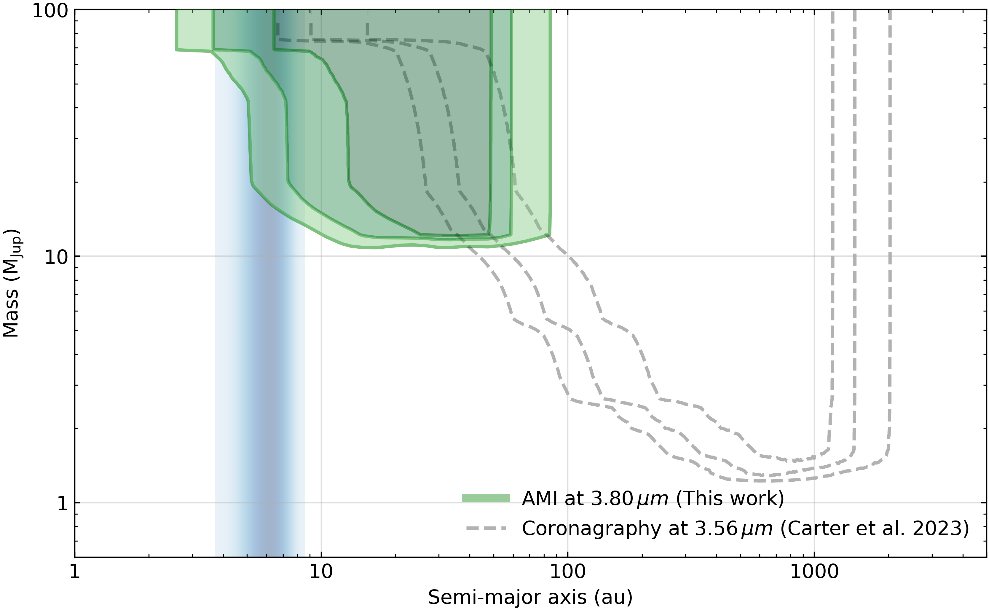
Figure 8: Detection probability maps (contours of 30%, 68% and 90%) for JWST observations, shown with water frost lines for the star HIP 65426: green shows AMI in F380M filter and the grey dashed lines show coronagraphy in the F356W filter. AMI reaches water frost line separations, shown by the vertical blue gradient, probing separations which is an essentially unexplored parameter space.

The Exoplanet Detection Map Calculator (Exo-DMC, Bonavita, 2020) was used to estimate a detection probability map using the mass sensitivity limits. This tool uses a Monte Carlo approach to compare the instrument detection limits with a simulated, synthetic population of planets with varying orbital geometries around a given star to estimate the probability of detection of a companion of a given mass and semi-major axis. This information is then summarised in a detection probability map. This Python language tool is an adaptation of the previously existing code MESS (Multi-purpose Exoplanet Simulation System, Bonavita et al., 2012).

Figure 8 shows the detection probability maps for the dataset described in this study (AMI at $3.80\,\rm{\mu m}$), as well as one for the coronagraphic observations of the same target obtained at a comparable wavelength ($3.56\,\rm{\mu m}$) described in Carter et al. (2023). The figure also shows the spatial extent of the the water frost line for the star and was calculated using methodology discussed in Ray et al. (2023) and Vigan et al. (2021). This was done by calculating the extent of the water frost line using the evaporation temperature of $20\,\rm{K}$ from Öberg et al. (2011), a parametric disk temperature profile from Lewis (1974) and observations of protoplanetary disks from Andrews & Williams (2005, 2007a, 2007b). Since the location of the water frost line has uncertainties on it, a gradient region demarcated by the frost line of a B-type star and an F-type star (within one spectral type of HIP 65426, an A-type star) is plotted. The darkest region is the halfway point between the two extremities and the gradient decreases linearly on either side. This is represented in a logarithmic scale in the figure. The figure clearly shows the exquisite capability of JWST/NIRISS/AMI to detect companions at mid-infrared wavelengths in a completely new orbital parameter space. This can also be seen in Figure 9 where JWST/NIRISS/AMI probes a completely different parameter space when compared to VLT/SPHERE/IRDIS observations at H-band ($1.6\,\rm{\mu m}$, Chauvin et al., 2017).

In this study we detect no additional companions but, Figure 8 clearly exhibits the capability of the AMI mode for the investigation of an unexplored parameter space of stellar systems with previously known companions. Figure 4 of Chauvin et al. (2017) shows that for this planetary system, regions ${\lesssim}20\,\rm{au}$, are inaccessible by VLT/SPHERE. In Figure 8, we rule out the existence of any additional companions ${\gtrsim}10\,\rm{M\textsubscript{Jup}}$ at separations ${\sim}10{-}20\,\rm{au}$ around the host star. These observations hence provide sensitivity inside of the classical IWAs of JWST’s conventional coronagraphs.

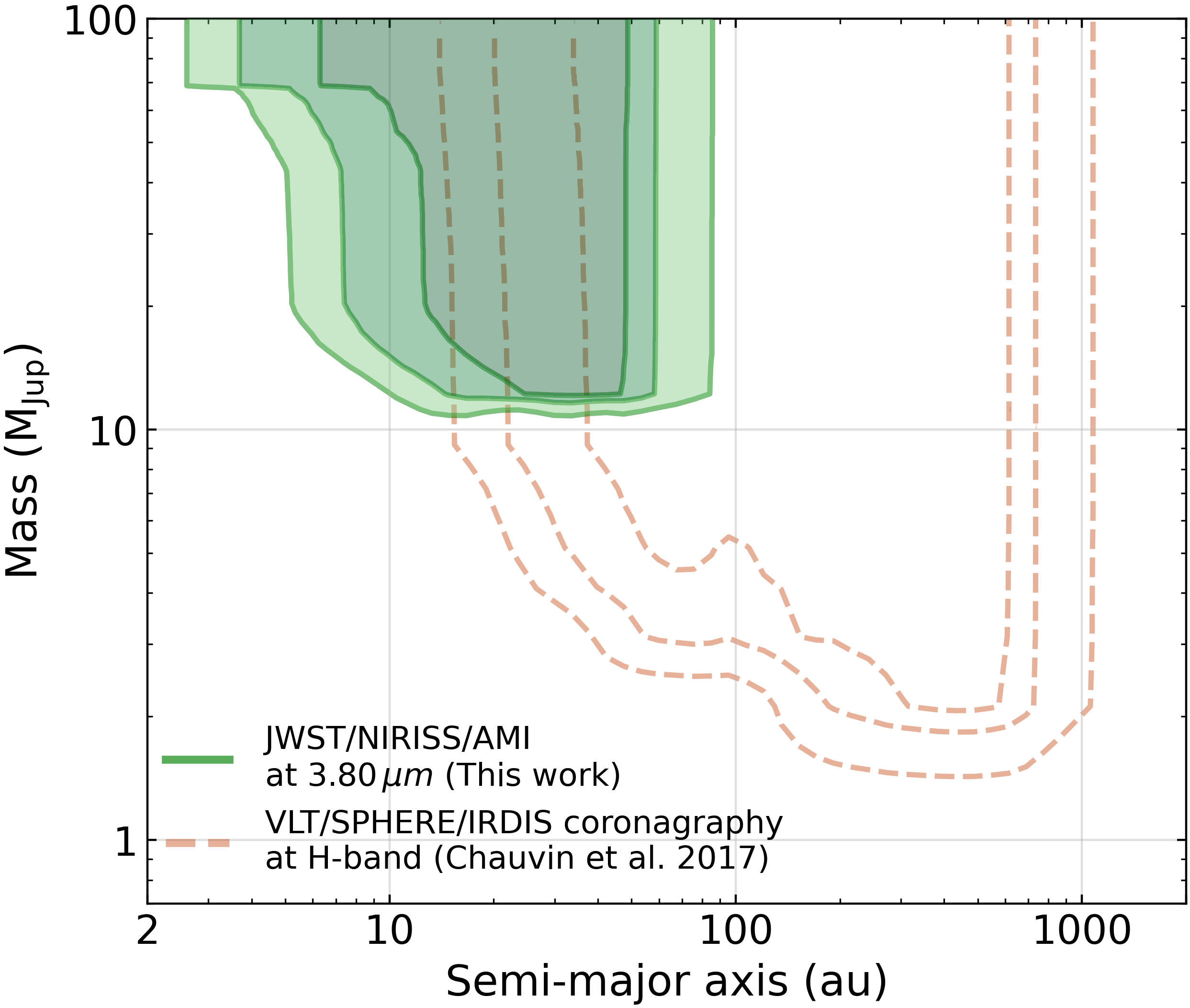
Figure 9: Detection probability maps (contours of 30%, 68% and, 90%) for the AMI observation in F380M filter with JWST/NIRISS, compared with the coronagraphic H band observations obtained with VLT/SPHERE/IRDIS (Chauvin et al., 2017), for the star HIP 65426.

6 Conclusions

In this study, we have demonstrated that the AMI mode with JWST/NIRISS accesses a completely new parameter space (separations of ${\sim}0.1{\arcsec}{-}0.4{\arcsec}$), a region which is only accessible at lower contrast from the ground, and inaccessible using the conventional coronagraphs on JWST. This is evident from Figures 8 and 9 which exhibit that with JWST/NIRISS/AMI, companions at Solar System planetary scales (as close in as ${\sim}10\,\rm{au}$) can be accessed.

Going forward, this mode will be the prime technique to detect companions around stars in the closest star forming regions at close-in separations. The number of stars in young moving groups available for planet searches is limited to ${\sim}100$ targets (for example in the moving groups of $\beta$ Pictoris and TW Hydrae, Ray et al., 2023). However, targeting stars in the Taurus-Auriga or Scorpius-Centaurus associations (which HIP 65426 is a member of), increases the number of such available targets by ${\sim}1{-}2$ orders of magnitude since these associations are potentially rich in thousands of such targets. Opening up the possibility to probe the members in these star formation regions would mean that many promising targets (e.g., those with debris disks, evidence for accretion or protoplanets using ALMA gas kinematics, etc.) can be probed. These targets could be part of future JWST (and ELT) observations.

This mode can also be used to find planets in systems which have previously known companions. The characterisation of the multiplicity of PMCs around nearby stars would be incomplete without probing inner regions, which JWST/NIRISS/AMI can access. Previous studies (Marois et al., 2010; Wagner et al., 2019; Nowak et al., 2020; Hinkley et al., 2023) have shown that additional companions at close in separations can be found in systems that already have a known companion. This is beyond the capabilities of conventional coronagraphs on JWST due to their relatively poor IWAs. Hence observations in future cycles using JWST/NIRISS/AMI will shed some light on this unexplored piece of parameter space.

The angular parameter space (${\sim}100{-}300\,\rm{mas}$, see Figure 6) accessible with JWST/AMI for the case of members in nearby stellar associations, overlaps the peak sensitivity of current and future ground-based interferometers such as GRAVITY (Lacour et al., 2019; Nowak et al., 2020) and BiFROST (Kraus et al., 2022). These interferometers can measure dynamical masses of PMCs with high precision (up to ${\sim 10\%}$) over a short portion of their orbit (e.g. Hinkley et al., 2023). The combination of the measurements of precise dynamical masses and the PMC brightness at ${\sim}3{-}5\,\rm{\mu m}$ (near the peak of their SED, which gives tightly constrained measurements of bolometric luminosity) is exceedingly powerful for constraining atmospheric and evolutionary models that are highly uncertain at young ages (see Figure 11, Ray et al., 2023). In addition to this, the obtained contrast limits (in Figures 6 and 7) will also access the expected luminosities of circumplanetary disks whose spectral energy distributions can be used to inform planet formation timescales and exomoon formation. Through these applications and more, NIRISS AMI observations in future cycles will provide new, direct constraints on planet formation and evolution.

References

- Andrews & Williams (2005) Andrews, S. M., & Williams, J. P. 2005, ApJ, 631, 1134, doi: 10.1086/432712
- Andrews & Williams (2007a) —. 2007a, ApJ, 659, 705, doi: 10.1086/511741
- Andrews & Williams (2007b) —. 2007b, ApJ, 671, 1800, doi: 10.1086/522885
- Baldwin et al. (1986) Baldwin, J. E., Haniff, C. A., Mackay, C. D., & Warner, P. J. 1986, Nature, 320, 595, doi: 10.1038/320595a0
- Baraffe et al. (2003) Baraffe, I., Chabrier, G., Barman, T. S., Allard, F., & Hauschildt, P. H. 2003, A&A, 402, 701, doi: 10.1051/0004-6361:20030252
- Barman et al. (2011) Barman, T. S., Macintosh, B., Konopacky, Q. M., & Marois, C. 2011, ApJ, 733, 65, doi: 10.1088/0004-637X/733/1/65
- Bonavita (2020) Bonavita, M. 2020, Exo-DMC: Exoplanet Detection Map Calculator. http://ascl.net/2010.008
- Bonavita et al. (2012) Bonavita, M., Chauvin, G., Desidera, S., et al. 2012, A&A, 537, A67, doi: 10.1051/0004-6361/201116852
- Bonneau et al. (2006) Bonneau, D., Clausse, J. M., Delfosse, X., et al. 2006, A&A, 456, 789, doi: 10.1051/0004-6361:20054469
- Bushouse et al. (2022) Bushouse, H., Eisenhamer, J., Dencheva, N., et al. 2022, spacetelescope/jwst: JWST 1.6.2, 1.6.2, Zenodo, Zenodo, doi: 10.5281/zenodo.6984366
- Carter et al. (2023) Carter, A. L., Hinkley, S., Kammerer, J., et al. 2023, ApJ, 951, L20, doi: 10.3847/2041-8213/acd93e
- Chauvin et al. (2017) Chauvin, G., Desidera, S., Lagrange, A. M., et al. 2017, A&A, 605, L9, doi: 10.1051/0004-6361/201731152
- Cheetham et al. (2016) Cheetham, A. C., Girard, J., Lacour, S., et al. 2016, in Society of Photo-Optical Instrumentation Engineers (SPIE) Conference Series, Vol. 9907, Optical and Infrared Interferometry and Imaging V, ed. F. Malbet, M. J. Creech-Eakman, & P. G. Tuthill, 99072T, doi: 10.1117/12.2231983
- Cheetham et al. (2019) Cheetham, A. C., Samland, M., Brems, S. S., et al. 2019, A&A, 622, A80, doi: 10.1051/0004-6361/201834112
- Currie et al. (2023) Currie, T., Brandt, G. M., Brandt, T. D., et al. 2023, Science, 380, 198, doi: 10.1126/science.abo6192
- Doyon et al. (2012) Doyon, R., Hutchings, J. B., Beaulieu, M., et al. 2012, in Society of Photo-Optical Instrumentation Engineers (SPIE) Conference Series, Vol. 8442, Space Telescopes and Instrumentation 2012: Optical, Infrared, and Millimeter Wave, ed. M. C. Clampin, G. G. Fazio, H. A. MacEwen, & J. Oschmann, Jacobus M., 84422R, doi: 10.1117/12.926578
- Doyon et al. (2023) Doyon, R., Willott, C. J., Hutchings, J. B., et al. 2023, arXiv e-prints, arXiv:2306.03277, doi: 10.48550/arXiv.2306.03277
- Foreman-Mackey et al. (2013) Foreman-Mackey, D., Hogg, D. W., Lang, D., & Goodman, J. 2013, PASP, 125, 306, doi: 10.1086/670067
- Gardner et al. (2006) Gardner, J. P., Mather, J. C., Clampin, M., et al. 2006, Space Sci. Rev., 123, 485, doi: 10.1007/s11214-006-8315-7
- Gardner et al. (2023) Gardner, J. P., Mather, J. C., Abbott, R., et al. 2023, PASP, 135, 068001, doi: 10.1088/1538-3873/acd1b5
- Greenbaum et al. (2015) Greenbaum, A. Z., Pueyo, L., Sivaramakrishnan, A., & Lacour, S. 2015, ApJ, 798, 68, doi: 10.1088/0004-637X/798/2/68
- Haniff et al. (1987) Haniff, C. A., Mackay, C. D., Titterington, D. J., Sivia, D., & Baldwin, J. E. 1987, Nature, 328, 694, doi: 10.1038/328694a0
- Hinkley et al. (2015) Hinkley, S., Kraus, A. L., Ireland, M. J., et al. 2015, ApJ, 806, L9, doi: 10.1088/2041-8205/806/1/L9
- Hinkley et al. (2022) Hinkley, S., Carter, A. L., Ray, S., et al. 2022, PASP, 134, 095003, doi: 10.1088/1538-3873/ac77bd
- Hinkley et al. (2023) Hinkley, S., Lacour, S., Marleau, G. D., et al. 2023, A&A, 671, L5, doi: 10.1051/0004-6361/202244727
- Hirata & Choi (2020) Hirata, C. M., & Choi, A. 2020, PASP, 132, 014501, doi: 10.1088/1538-3873/ab44f7
- Ireland (2013) Ireland, M. J. 2013, MNRAS, 433, 1718, doi: 10.1093/mnras/stt859
- Kammerer et al. (2019) Kammerer, J., Ireland, M. J., Martinache, F., & Girard, J. H. 2019, MNRAS, 486, 639, doi: 10.1093/mnras/stz882
- Kammerer et al. (2023) Kammerer, J., Cooper, R. A., Vandal, T., et al. 2023, PASP, 135, 014502, doi: 10.1088/1538-3873/ac9a74
- Konopacky et al. (2013) Konopacky, Q. M., Barman, T. S., Macintosh, B. A., & Marois, C. 2013, Science, 339, 1398, doi: 10.1126/science.1232003
- Kraus & Ireland (2012) Kraus, A. L., & Ireland, M. J. 2012, ApJ, 745, 5, doi: 10.1088/0004-637X/745/1/5
- Kraus et al. (2022) Kraus, S., Mortimer, D., Chhabra, S., et al. 2022, in Society of Photo-Optical Instrumentation Engineers (SPIE) Conference Series, Vol. 12183, Optical and Infrared Interferometry and Imaging VIII, ed. A. Mérand, S. Sallum, & J. Sanchez-Bermudez, 121831S, doi: 10.1117/12.2627973
- Lacour et al. (2019) Lacour, S., Dembet, R., Abuter, R., et al. 2019, A&A, 624, A99, doi: 10.1051/0004-6361/201834981
- Lewis (1974) Lewis, J. S. 1974, Science, 186, 440, doi: 10.1126/science.186.4162.440
- Marois et al. (2010) Marois, C., Zuckerman, B., Konopacky, Q. M., Macintosh, B., & Barman, T. 2010, Nature, 468, 1080, doi: 10.1038/nature09684
- Miles et al. (2023) Miles, B. E., Biller, B. A., Patapis, P., et al. 2023, ApJ, 946, L6, doi: 10.3847/2041-8213/acb04a
- Monnier et al. (2007) Monnier, J. D., Tuthill, P. G., Danchi, W. C., Murphy, N., & Harries, T. J. 2007, ApJ, 655, 1033, doi: 10.1086/509873
- Nowak et al. (2020) Nowak, M., Lacour, S., Lagrange, A. M., et al. 2020, A&A, 642, L2, doi: 10.1051/0004-6361/202039039
- Öberg et al. (2011) Öberg, K. I., Murray-Clay, R., & Bergin, E. A. 2011, ApJ, 743, L16, doi: 10.1088/2041-8205/743/1/L16
- Phillips et al. (2020) Phillips, M. W., Tremblin, P., Baraffe, I., et al. 2020, A&A, 637, A38, doi: 10.1051/0004-6361/201937381
- Ray et al. (2023) Ray, S., Hinkley, S., Sallum, S., et al. 2023, MNRAS, 519, 2718, doi: 10.1093/mnras/stac3425
- Readhead et al. (1988) Readhead, A. C. S., Nakajima, T. S., Pearson, T. J., et al. 1988, AJ, 95, 1278, doi: 10.1086/114724
- Rigby et al. (2022) Rigby, J., Perrin, M., McElwain, M., et al. 2022, arXiv e-prints, arXiv:2207.05632. https://arxiv.org/abs/2207.05632
- Sallum et al. (2022) Sallum, S., Ray, S., & Hinkley, S. 2022, in Society of Photo-Optical Instrumentation Engineers (SPIE) Conference Series, Vol. 12183, Optical and Infrared Interferometry and Imaging VIII, ed. A. Mérand, S. Sallum, & J. Sanchez-Bermudez, 121832M, doi: 10.1117/12.2630401
- Sallum et al. (2023) Sallum, S., Ray, S., & Kammerer, J. e. a. 2023, ApJ
- Sallum et al. (2019) Sallum, S., Bailey, V., Bernstein, R. A., et al. 2019, BAAS, 51, 527. https://arxiv.org/abs/1903.05319
- Saumon & Marley (2008) Saumon, D., & Marley, M. S. 2008, ApJ, 689, 1327, doi: 10.1086/592734
- Sivaramakrishnan et al. (2009) Sivaramakrishnan, A., Tuthill, P. G., Ireland, M. J., et al. 2009, in Society of Photo-Optical Instrumentation Engineers (SPIE) Conference Series, Vol. 7440, Techniques and Instrumentation for Detection of Exoplanets IV, ed. S. B. Shaklan, 74400Y, doi: 10.1117/12.826633
- Sivaramakrishnan et al. (2012) Sivaramakrishnan, A., Lafrenière, D., Ford, K. E. S., et al. 2012, in Society of Photo-Optical Instrumentation Engineers (SPIE) Conference Series, Vol. 8442, Space Telescopes and Instrumentation 2012: Optical, Infrared, and Millimeter Wave, ed. M. C. Clampin, G. G. Fazio, H. A. MacEwen, & J. Oschmann, Jacobus M., 84422S, doi: 10.1117/12.925565
- Sivaramakrishnan et al. (2023a) Sivaramakrishnan, A., Tuthill, P., Lloyd, J. P., et al. 2023a, PASP, 135, 015003, doi: 10.1088/1538-3873/acaebd
- Sivaramakrishnan et al. (2023b) —. 2023b, PASP, 135, 015003, doi: 10.1088/1538-3873/acaebd
- Soulain et al. (2020) Soulain, A., Sivaramakrishnan, A., Tuthill, P., et al. 2020, in Society of Photo-Optical Instrumentation Engineers (SPIE) Conference Series, Vol. 11446, Society of Photo-Optical Instrumentation Engineers (SPIE) Conference Series, 1144611, doi: 10.1117/12.2560804
- Spiegel & Burrows (2012) Spiegel, D. S., & Burrows, A. 2012, ApJ, 745, 174, doi: 10.1088/0004-637X/745/2/174
- Spiegel et al. (2011) Spiegel, D. S., Burrows, A., & Milsom, J. A. 2011, ApJ, 727, 57, doi: 10.1088/0004-637X/727/1/57
- Stolker et al. (2020) Stolker, T., Quanz, S. P., Todorov, K. O., et al. 2020, A&A, 635, A182, doi: 10.1051/0004-6361/201937159
- Tokovinin et al. (2010) Tokovinin, A., Cantarutti, R., Tighe, R., et al. 2010, PASP, 122, 1483, doi: 10.1086/657903
- Tuthill et al. (2001) Tuthill, P. G., Monnier, J. D., & Danchi, W. C. 2001, Nature, 409, 1012, doi: 10.1038/35059014
- Tuthill et al. (2000) Tuthill, P. G., Monnier, J. D., Danchi, W. C., Wishnow, E. H., & Haniff, C. A. 2000, PASP, 112, 555, doi: 10.1086/316550
- Vigan et al. (2021) Vigan, A., Fontanive, C., Meyer, M., et al. 2021, A&A, 651, A72, doi: 10.1051/0004-6361/202038107
- Wagner et al. (2019) Wagner, K., Apai, D., & Kratter, K. M. 2019, ApJ, 877, 46, doi: 10.3847/1538-4357/ab1904