Strong enhancement of superconductivity on finitely ramified fractal lattices

Abstract

Using the Sierpiński gasket (triangle) and carpet (square) lattices as examples, we theoretically study the properties of fractal superconductors. For that, we focus on the phenomenon of $s$-wave superconductivity in the Hubbard model with attractive on-site potential and employ the Bogoliubov-de Gennes approach and the theory of superfluid stiffness. For the case of the Sierpiński gasket, we demonstrate that fractal geometry of the underlying crystalline lattice can be strongly beneficial for superconductivity, not only leading to a considerable increase of the critical temperature $T_{c}$ as compared to the regular triangular lattice but also supporting macroscopic phase coherence of the Cooper pairs. In contrast, the Sierpiński carpet geometry does not lead to pronounced effects, and we find no substantial difference as compared with the regular square lattice. We conjecture that the qualitative difference between these cases is caused by different ramification properties of the fractals.

Quantum dynamics on artificial fractal lattices is a novel research direction that emerged several years ago as a result of the recent developments of experimental techniques such as molecular assembly mol_ass , supramolecular templating sup_templ , scanning tunneling microscopy STM (STM), and high-energy-beam lithography lithography , which opened a way to manufacture nanoscale fractal-shaped atomic arrays in a lab on demand. The interest in fractal quantum systems is driven by their unique combination of features untypical for conventional solid-state structures. Foremost, due to their fractional Hausdorff dimension, fractals are geometric entities interpolating between regular one-dimensional wires and two-dimensional layers. Given the decisive role of spatial dimension for physical properties of materials and engineered structures, this can potentially lead to novel physics impossible in integer dimensions. Discrete scale invariance is another attribute of fractals that can strongly affect their spectra of quantum excitations and observable properties Askar_spectra_1 ; Askar_spectra_2 ; Askar_spectra_3 . Finally, fractality can be viewed as a highly peculiar type of defect distribution in a two-dimensional crystal that has a regular geometric structure and is akin neither to clean translationally invariant lattices nor to disorder.

Theoretically, fractal lattices have been mainly explored at the level of classical phase transitions Gefen1 ; Gefen2 ; Gefen3 and single-particle quantum dynamics, where solid knowledge has already been acquired Kadanoff ; Laskin ; quantum_walks ; vanVeen . Electronic band structures of certain artificial fractal crystals have been theoretically derived and measured in experiments fractal_bands . Non-equilibrium propagation of light through fractal lattices has been studied, and the mathematical theory of diffusion on them has been developed fractal_light . Topologically protected phases were shown both theoretically fractal_HOT ; Neupert_topology ; fractal_topology and experimentally Canyellas to exist in fractal structures, and even the existence of a novel class of topological states impossible in regular crystalline lattices – topological random fractals – has been conjectured topological_random_fractals . Researchers have analyzed electron transport on fractals and related conductance fluctuations in fractal structures to their Hausdorff dimensions fractal_conductance , and predicted plasmon confinement in finitely ramified lattices westerhout_plasmons .

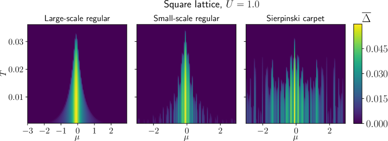
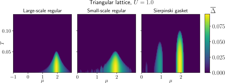
Figure 1: $T-\mu$ phase diagrams of the attractive Hubbard model on regular lattices and fractal structures. For both the triangular and the square geometries, the BdG equations have been solved self-consistently for three cases. Left column: large-scale lattices mimicking the thermodynamic limit – square-shaped samples (for both geometries) with side length $L=1000$ and periodic boundary conditions. Middle column: small-scale samples with regular lattice geometry; for the square lattice, the sample is of square shape (side length $L=27$), and for the triangular one – of the triangular shape (side length $L=33$), both with open boundary conditions. Right column: Sierpiński carpet (side length $L=27$) and gasket (side length $L=33$) with open boundary conditions.

In the domain of correlated systems, fractals have been explored to much lesser extent. Some results have been obtained regarding formation of fractal patterns in otherwise regular settings. Fractal Fermi surfaces were shown to emerge in the band structure of non-Hermitian models nodal_bands . For driven one-dimensional systems, formation of quantum states with fractional Khemani and explicitly fractal-shaped scaling of entanglement entropy Ageev was demonstrated. The few undertaken attempts to study fractal geometries hosting many-body quantum dynamics led to highly promising results, but only particular cases have been investigated. For example, it was shown that the interplay of fractality and interactions can amplify the robustness of the fractional quantum Hall phase Nielsen-1 ; Nielsen-2 or host spin liquid phases fractal_SL . Auxiliary-field quantum Monte Carlo study of the Sierpiński gasket Hubbard model showed the existence of localized states and ferrimagnetic order AFQMC . In the realm of superconductivity, it was shown both theoretically and experimentally that disorder-induced multifractality enhances superconductivity in thin films Burmistrov-1 ; Burmistrov-2 ; multifrac_exp . However, these results account only for the average scale invariance of disorder, and understanding the possible role of discrete self-similarity and highly symmetric geometry of regular fractal lattices, such as the Sierpiński gaskets and carpets, remains an open problem. Here, we make the first step in this direction and study superconductors with regular fractal geometry. We pursue this analysis motivated by the hope that due to the regular, though non-crystalline, geometric structure of fractals one can hopefully gain benefits of disorder, such as the increase in the critical temperature of formation of individual Cooper pairs disorder_SC , without suffering from the destructive self-interference and losing the long-range phase coherence of the superconducting condensate.

For that, we consider the minimal model known to host superconductivity – the Hubbard model with on-site attractive interactions:

$$H=t\sum_{\langle i,j\rangle\sigma}c^{\dagger}_{i\sigma}c_{j\sigma}-\mu\sum_{i\sigma}n_{i\sigma}-U\sum_{i}n_{i\uparrow}n_{i\downarrow}$$ (1)

where $c^{\dagger}_{i\sigma},\,c_{i\sigma}$ are creation and annihilation operators of fermion with spin $\sigma=\uparrow,\downarrow$ at site $i$, $n_{i\sigma}=c^{\dagger}_{i\sigma}c_{i\sigma}$ is the particle number operator, $t=-1$ is the nearest-neighbor hopping, $\mu$ is the chemical potential, and $U>0$ is the strength of attractive on-site interactions.

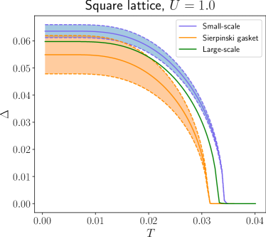
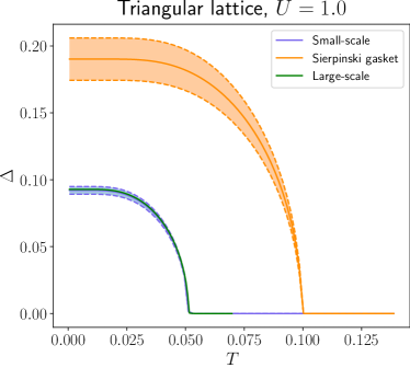
Figure 2: Spatial average of the Cooper pair condensate $\overline{\Delta}$ as a function of temperature $T$ at $U=1$ and optimal chemical potential ($\mu=0$ for the square lattice, and $\mu=2$ for the triangular one). For each parental geometry, three cases are shown – regular lattice in the thermodynamic limit (green lines; simulated as square-shaped unit cells with side length $L=1000$ and periodic boundary conditions), small-scale sample with regular structure and open boundary conditions (purple lines; simulated as a square cell with side length $L=27$ and right triangular cell with side length $L=33$ correspondingly), and finite-size fractals with open boundary conditions (orange lines; the same side lengths as for regular small-scale lattices). Shaded regions show spatial standard deviations of $\Delta$ from $\overline{\Delta}$ across the lattice.

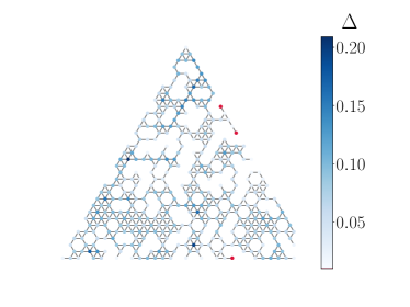
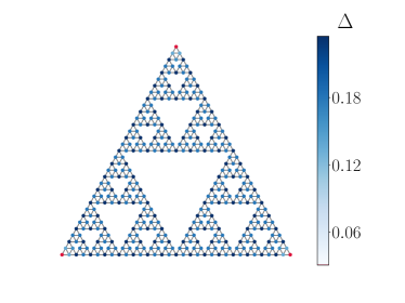
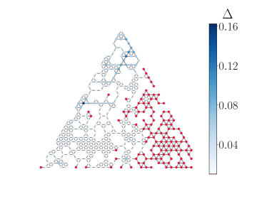
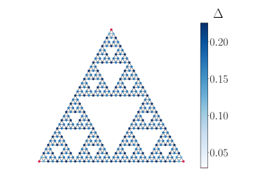
Figure 3: Cooper pair condensate $\Delta$ at $U=1.0$, chemical potential $\mu=2.0$, temperature $T=0.005$ for the top figures, and $T=0.05$ (around $T_{c}$ of the undeformed lattice) for the bottom ones. Two structures are shown – the triangular sample with the disorder ($30\%$ of deleted sites) and the Sierpiński gasket of depth $4$. The sites with $\Delta<0.01$ are indicated by red color.

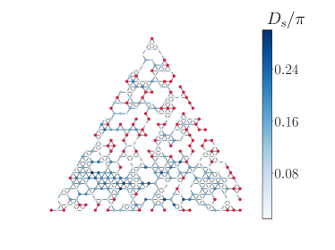
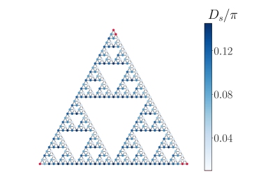
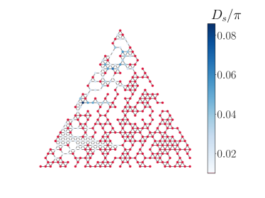
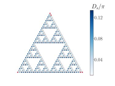
Figure 4: The superfluid density $D_{s}/\pi$ at $U=1.0$, chemical potential $\mu=2.0$, temperature $T=0.005$ for the top figures, and $T=0.05$ (around $T_{c}$ of the undeformed lattice) for the bottom ones. Two structures are shown – triangular sample with the disorder ($30\%$ of deleted sites) and the Sierpiński gasket of depth $4$. The sites with $D_{s}/\pi<0.01$ are indicated by red color.

Our first goal is to compute the real-space profile of the superconducting condensate across the parametric space of the model. We do that within the self-consistent Bogoliubov-de Gennes approach BdG1 ; BdG2 ; Book . Within the coherent potential approximation (CPA) for on-site-disordered superconductor, this relatively simple approach Zittartz1 ; Zittartz2 was shown to lead to the same results as the complete Eliashberg theory for electron-phonon interactions MK_Anokhin . Therefore one can hope that this approach may be sufficient also for our situation.

We apply the mean-field approximation:

$$n_{i\uparrow}n_{i\downarrow}\approx\langle c_{i\uparrow}c_{i\downarrow}\rangle c^{\dagger}_{i\uparrow}c^{\dagger}_{i\downarrow}+\langle c^{\dagger}_{i\uparrow}c^{\dagger}_{i\downarrow}\rangle c_{i\uparrow}c_{i\downarrow}.$$ (2)

Introducing the local pairing amplitude $\Delta_{i}$, the mean-field Hamiltonian can be rewritten as follows

$$H=t\sum_{\langle i,j\rangle\sigma}c^{\dagger}_{i\sigma}c_{j\sigma}-\mu\sum_{i\sigma}n_{i\sigma}+\sum_{i}[\Delta_{i}c^{\dagger}_{i\uparrow}c^{\dagger}_{i\downarrow}+\Delta^{*}_{i}c_{i\uparrow}c_{i\downarrow}],$$ (3)

with self-consistency conditions given by

$$\Delta_{i}=|U|\langle c_{i\uparrow}c_{i\downarrow}\rangle$$ (4)

$$\langle n_{i\sigma}\rangle=\langle c^{\dagger}_{i\sigma}c_{i\sigma}\rangle.$$

To bring the mean-field Hamiltonian to single–particle form, we apply the Bogoliubov transformation

$$c^{\dagger}_{i\uparrow}=\sum_{n(E_{n}\geq 0)}(u^{n*}_{i\uparrow}\gamma^{\dagger}_{n\uparrow}-v^{n}_{i\uparrow}\gamma_{n\downarrow}),$$ (5)

$$c^{\dagger}_{i\downarrow}=\sum_{n(E_{n}\geq 0)}(u^{n*}_{i\downarrow}\gamma^{\dagger}_{n\downarrow}-v^{n}_{i\downarrow}\gamma_{n\uparrow})$$

where $\gamma_{n}$ and $\gamma^{\dagger}$ are quasiparticle operators satisfying the fermionic anti-commutation relations and the relation:

$$\langle\gamma^{\dagger}_{n\sigma}\gamma_{n\sigma}\rangle=\frac{1}{\exp(E_{n\sigma}/k_{B}T)+1}.$$ (6)

The Fermi-Dirac distribution function is denoted as $f(E_{n\sigma})$ in what follows .

In the new basis, the eigenvalue equation acquires the form

$$\begin{pmatrix}\hat{K}&\hat{\Delta}\\ \hat{\Delta}^{*}&-\hat{K}\end{pmatrix}\begin{pmatrix}u^{n}_{\uparrow}\\ v^{n}_{\downarrow}\end{pmatrix}=E_{n\uparrow}\begin{pmatrix}u^{n}_{\uparrow}\\ v^{n}_{\downarrow}\end{pmatrix},$$ (7)

where $\hat{K}$ is the matrix representing the free part of the Hamiltonian, and $\hat{\Delta}=\mbox{diag}(\Delta_{1},\dots\Delta_{N})$ with $N$ being the total number of lattice sites. Due to the absence of spin-orbit coupling and real-valuedness of the eigenfunctions, the other vector $(u_{n\downarrow},v_{n\uparrow})^{T}$ satisfies exactly the same equation. Hence, we need to solve the equation only for one of them, and from now on we omit the spin indices.

The self-consistency conditions are then:

$$\Delta_{i}=\frac{|U|}{2}\sum_{n}u^{n}_{i}v^{n*}_{i}\tanh(\frac{E_{n}}{2k_{B}T}),$$ (8)

$$\langle n_{i}\rangle=\sum_{n}[|u^{n}_{i}|^{2}f(E_{n})+|v^{n}_{i}|^{2}f(-E_{n})],,$$ (9)

where the sums run over both the positive and the negative parts of the spectrum, and we solve Eqs. (7)-(9) iteratively.

To unveil the effects of fractal geometry on superconductivity, for each point $(T,\mu,U)$ in the space of parameters, we solve the equations for three cases. First, for a regular lattice (either square or triangular) with large linear size $L=1000$ ($N=L^{2}$) and periodic boundary conditions – to reconstruct the phase diagram in the thermodynamic limit. Secondly, for a regular lattice, but with a smaller linear size $L=27$ and open boundary conditions – to see how the finite-size effects affect the phase diagram. Finally, we solve the equations for the fractal structures with side length $L=27$ (the Sierpiński carpet in the case of the parental square lattice, and the gasket for the parental triangular lattice). The results for $U=1.0$ are shown in Fig. 1. From these pictures, it is clear that fractal geometry brings more than just finite-size effects to the table. In the case of the Sierpiński carpet, it broadens the superconducting dome and makes its structure highly irregular, but has little effect on the optimal critical temperature, even lowering it a bit. On the contrary, the gasket geometry leads to a strong increase of maximal $T_{c}$, doubling it for the chosen value of attractive coupling Babaev (in App. B, we provide results for other values of $U$). One-dimensional sections of the phase diagrams at optimal values of chemical potential are shown in Fig.2, and the spatial profile of condensate in Fig.3 (for the carpet, it is shown in App. C).

However, the enhancement of critical temperature does not automatically imply that superconductivity survives at higher temperatures as a global phenomenon. It is still possible that fractal geometry makes individual Cooper pairs more robust to thermal fluctuations, but breaks the long-range coherence of the global superconducting condensate and hence prohibits the large-scale supercurrent flow through the sample (a possible scenario for disordered superconductors disorder_kill_SC ; Feigelman ). In the bottom panel of Fig.3, we see that non-zero condensate $\Delta$ survives across the lattice for both the disordered and the fractal systems at the temperature that would be critical for the undeformed sample, indicating an increase in $T_{c}$ in both cases. The long-range coherence can be analyzed by computing the superfluid stiffness of the system in the presence of an external electric field. Then, the condition for the existence of a supercurrent flow between two points of the sample is the existence of a line connecting them along which the superfluid stiffness is non-zero everywhere.

Assume that the electric field $E_{x}$ is applied along the $x$-axis (rightwards along the lower leg of the triangle in Figs. 3, 4). The superfluid stiffness is then given by Scalapino :

$$\frac{D_{s}}{\pi}=\Pi_{xx}(q_{x}=0,q_{y}\to 0,\omega=0)-\langle K_{x}\rangle,$$ (10)

where $\Pi_{xx}$ is the retarded current-current correlation function, $\omega$ and ${\bf q}$ are the frequency and the wave vector of the applied electric field correspondingly, and $\langle K_{x}\rangle$ is the kinetic energy density of electrons moving in the direction of the applied field. Explicit form of the r.h.s. of (10) used for numerical computations is given in App. A.

We computed the on-site superfluid stiffness $D_{s}/\pi$ for the Sierpiński gasket and for a disordered sample of the triangular lattice with $\sim 30\%$ of sites removed (so that both lattices have approximately the same number of sites). The results are shown in Fig. 4. As one can see, for the disordered sample, the profile of $D_{s}/\pi$ is highly irregular, and the stiffness vanishes in many points splitting the system into a number of disconnected superconducting islands and making the global flow of supercurrent through the sample impossible. On the other hand, for the Sierpiński gasket, $D_{s}/\pi=0$ only on the corner sites where the current induced by $E_{x}$ terminates, leaving the rest of the lattice a connected component capable of hosting a global current. The case of Sierpiński carpet is shown in App. C.

Our considerations demonstrate, on the proof-of-concept level, that a certain fractal geometry can lead to a considerable enhancement of superconductivity as compared to the original parental crystalline lattice. Here, we have analyzed it within a minimal framework, and several further steps are required to gain an in-depth understanding of this phenomenon. First of all, it should be noted that the effect of $T_{c}$ elevation for boundary states in regular crystalline superconductors has been recently discussed Babaev_boundary . Since fractal lattices have boundaries “everywhere” in the bulk, it is possible that a similar effect plays a certain role here. In this paper, we studied only the $s$-wave superconductivity, while superconducting condensates with other types of symmetry, such as $p$- or $d$-wave, can be affected by fractal geometries in different ways. This can be analyzed on the BdG mean-field level as well but in the extended attractive Hubbard model. The next natural steps will be to develop a complete Eliashberg theory of superconductivity in fractal geometries, and to employ more sophisticated real-space methods (real-space constrained random phase approximation real_space or variational finite-temperature Monte Carlo algorithms VMC1 ; VMC2 ) to study fractal superconductors in the regime of strong repulsive interactions in more realistic models such as the $t-t^{\prime}$ repulsive Hubbard model t-t-prime1 ; t-t-prime2 ; t-t-prime3 and to account for the long-range Coulomb interactions Coulomb1 ; Coulomb2 ; Coulomb3 . Should this phenomenon emerge in other regimes apart from those considered in this paper, it could define a new way to search for novel high-Tc superconductors based on engineered atomic deformations of lattice geometries of the natural crystalline superconductors.

Appendix A Derivation of the superfluid stiffness

Kinetic energy in (10) is defined by the following expression:

$$\langle K_{x}\rangle=\frac{1}{N}\sum_{l,\sigma}K_{l,\sigma,x}=-\frac{t}{N}\langle\sum_{l\sigma}\sum_{m}(x_{l}-x_{m})^{2}[c^{\dagger}_{k\sigma}c_{m\sigma}+c^{\dagger}_{l\sigma}c_{m\sigma}]\rangle,$$ (11)

where $N$ is the number of lattice sites, we set the lattice constant $a=1$, and the summation over index $m$ goes over the neighbors of the site $l$ with larger $x$ coordinate, $x_{m}>x_{l}$.

The retarded current-current correlator can be obtained by the analytical continuation from the expression written in the Matsubara frequencies, $\omega_{n}\to\omega+i\delta$:

$$\Pi_{xx}({\bf q},\omega_{n})=\frac{1}{N}\int^{\beta}_{0}e^{i\omega_{n}\tau}\langle j_{x}({\bf q},\tau)j_{x}(-{\bf q},0)\rangle,$$ (12)

where the current operator $j_{x}$ is defined as:

$$j_{x}=it\sum_{l\sigma}\sum_{m}e^{-i{\bf q}\cdot{\bf r_{l}}}(x_{m}-x_{l})[c^{\dagger}_{m\sigma}c_{l\sigma}-c^{\dagger}_{l\sigma}c_{m\sigma}],$$ (13)

with $\bf{r_{l}}$ being the Cartesian coordinates of the lattice sites.

After the Bogoliubov transformation, these terms acquire the following forms.

The kinetic energy expectation value:

$$\langle K_{x}\rangle=-\frac{2t}{N}\sum_{n,l}\sum_{m}(x_{m}-x_{l})^{2}[(u^{n*}_{m}u^{n}_{l}+u^{n*}_{l}u^{n}_{m})f(E_{n})+(v^{n*}_{m}v^{n}_{l}+v^{n*}_{l}v^{n}_{m})f(-E_{n})].$$ (14)

The current-current correlator:

$$\Pi_{xx}({\bf q},\omega_{n})=\frac{1}{N}\sum_{n_{1},n_{2}}\frac{A_{n_{1},n_{2}}({\bf q})[A^{*}_{n_{1},n_{2}}({\bf q})+D_{n_{1},n_{2}}(-{\bf q})]}{\omega+(E_{n_{1}}-E_{n_{2}})+i\delta}[f(E_{n_{1}})-f(E_{n_{2}})],$$ (15)

where $A_{n1,n_{2}}({\bf q})$ and $D_{n1,n_{2}}({\bf q})$ are defined as:

$$A_{n_{1},n_{2}}({\bf q})=2\sum_{l}e^{-i{\bf q}\cdot{\bf r}_{l}}\sum_{m}(x_{m}-x_{l})[u^{n_{1}*}_{m}u^{n_{2}}_{l}-u^{n_{1}*}_{l}u^{n_{2}}_{m}]$$ (16)

$$D_{n_{1},n_{2}}({\bf q})=2\sum_{l}e^{-i{\bf q}\cdot{\bf r}_{l}}\sum_{m}(x_{m}-x_{l})[v^{n_{1}*}_{m}v^{n_{2}}_{l}-v^{n_{1}*}_{l}v^{n_{2}}_{m}].$$ (17)

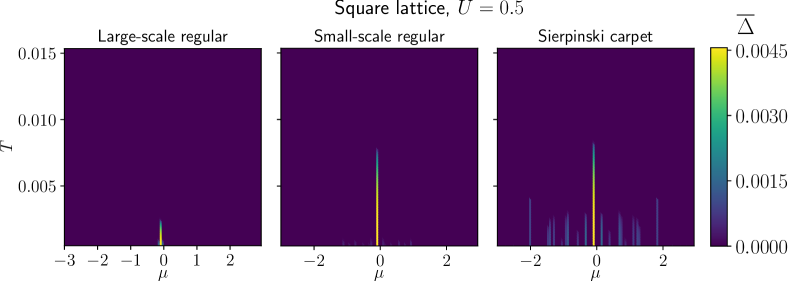
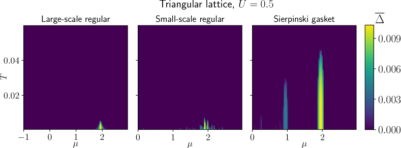
Figure 5: $T-\mu$ phase diagrams of the attractive Hubbard model on regular lattices and fractal structures at $U=0.5$. The description given in the caption of Fig.1 applies here.

To compute the superfluid stiffness, we first set $\omega=0$ in the Eq. (15), and then take the limit ${\bf q}\to 0$ obtaining:

$$\Pi_{xx}({\bf q}\to 0,\omega_{n})=\frac{1}{N}\sum_{n_{1},n_{2}}\frac{f(E_{n_{1}})-f(E_{n_{2}})}{E_{n_{1}}-E_{n_{2}}}A_{n_{1},n_{2}}({\bf q}\to 0)[A^{*}_{n_{1},n_{2}}({\bf q}\to 0)+D_{n_{1},n_{2}}({\bf q}\to 0)]$$ (18)

where, in the case of $E_{n_{1}}=E_{n_{2}}$, the prefactor should be calculated as $\partial_{E}f(E)$.

The stiffness computed from Eqs. (14) and (18) is averaged over the lattice sites. To calculate its spatial profile across the lattice, we need to avoid averaging over the sites by omitting the summations over $l$ in Eq. (14) and in the first $A_{n_{1},n_{2}}({\bf q})$ multiplier in the numerator of Eq. (18), as well as the normalizing $1/N$ factors. The local value of $\Pi_{xx}$ on site $l$ is given by:

$$\Pi_{xx}({\bf q},\omega_{n},l)=\sum_{n_{1},n_{2}}\frac{A^{\prime}_{n_{1},n_{2}}({\bf q},l)[A^{*}_{n_{1},n_{2}}({\bf q})+D_{n_{1},n_{2}}(-{\bf q})]}{\omega+(E_{n_{1}}-E_{n_{2}})+i\delta}[f(E_{n_{1}})-f(E_{n_{2}})]$$ (19)

with

$$A^{\prime}_{n_{1},n_{2}}({\bf q})=2e^{-i{\bf q}\cdot{\bf r}_{l}}\sum_{m}(x_{m}-x_{l})[u^{n_{1}*}_{m}u^{n_{2}}_{l}-u^{n_{1}*}_{l}u^{n_{2}}_{m}]$$ (20)

Appendix B Phase diagrams at different values of U

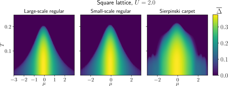
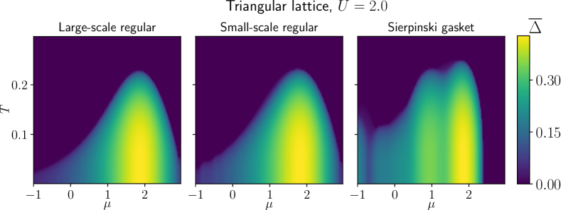
Figure 6: $T-\mu$ phase diagrams of the attractive Hubbard model on regular lattices and fractal structures at $U=2.0$. The description given in the caption of Fig.1 applies here.

In the main text, we took $U=1.0$, but it is also interesting to consider how fractal geometry affects $T_{c}$ in the regimes of stronger or weaker attraction. For $U=0.5$ and $U=2.0$, the phase diagrams are shown in Figs.5, 6. From this figures, it is clear that at lower values of $U$, where pairing is weak and $T_{c}$ is low, the gasket-type fractality leads to much stronger relative increase in $T_{c}$, while in the regime of very strong attraction this effect becomes negligible. One can speculate that it can be related to the smearing of the Cooper pairs over the fractal geometry. When attraction is weak and the coherence length is large, the Cooper pair embraces a larger part of the lattice, and there are a few iterations of the fractal inside the pair, alternating its properties. On the other hand, at strong attraction, the Cooper pair is compact and the role played by fractality reduces to local boundary effects.

Appendix C Spatial $\Delta$ and $D_{s}$ profiles on the Sierpiński carpet

While there seems to be no enhancement of superconductivity on the Sierpiński carpet as compared with the square lattice case, for the sake of completeness we plot spatial profiles of the Cooper pair condensate and the superfluid stiffness on the carpet and on the randomly disordered lattice with approximately the same number of removed sites. Those are shown in Figs. 7 and 8.

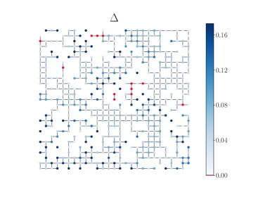
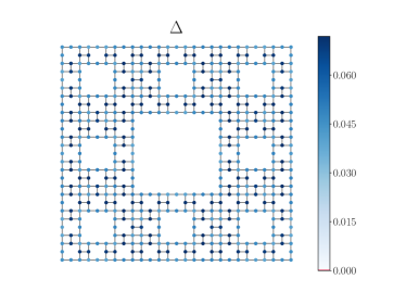
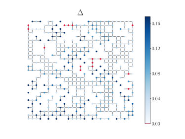
Figure 7: Cooper pair condensate $\Delta$ at $U=1.0$, chemical potential $\mu=0.0$, temperature $T=0.005$ for the top figures, and $T=0.025$ (around $T_{c}$ of the undeformed lattice) for the bottom ones. Two structures are shown – square sample with the disorder ($30\%$ of deleted sites) and the Sierpiński carpet of depth $3$. The sites with $\Delta<0.01$ are indicated by red color.

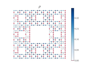
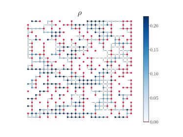
Figure 8: The superfluid density $\rho=D_{s}/\pi$ at $U=1.0$, chemical potential $\mu=0.0$, temperature $T=0.005$ for the top figures, and $T=0.025$ (around $T_{c}$ of the undeformed lattice) for the bottom ones. Two structures are shown – square sample with the disorder ($30\%$ of deleted sites) and the Sierpiński carpet of depth $3$. The sites with $D_{s}/\pi<0.01$ are indicated by red color.