$\Sigma_{\mathrm{SFR}}$–$M_{*}$ Diagram: A Valuable Galaxy Evolution Diagnostic to Complement (s)SFR–$M_{*}$ Diagrams

Abstract

The specific star formation rate (sSFR) is commonly used to describe the level of galaxy star formation (SF) and to select quenched galaxies. However, being a relative measure of the young-to-old population, an ambiguity in its interpretation may arise because a small sSFR can be either because of a substantial previous mass build up, or because SF is low. We show, using large samples spanning $0<z<2$, that the normalization of SFR by the physical extent over which SF is taking place (i.e., SFR surface density, $\Sigma_{\mathrm{SFR}}$) overcomes this ambiguity. $\Sigma_{\mathrm{SFR}}$ has a strong physical basis, being tied to the molecular gas density and the effectiveness of stellar feedback, so we propose $\Sigma_{\mathrm{SFR}}$–$M_{*}$ as an important galaxy evolution diagram to complement (s)SFR–$M_{*}$ diagrams. Using the $\Sigma_{\mathrm{SFR}}$–$M_{*}$ diagram we confirm the Schiminovich et al. (2007) result that the level of SF along the main sequence today is only weakly mass dependent—high-mass galaxies, despite their redder colors, are as active as blue, low-mass ones. At higher redshift, the slope of the “$\Sigma_{\mathrm{SFR}}$main sequence” steepens, signaling the epoch of bulge build-up in massive galaxies. We also find that $\Sigma_{\mathrm{SFR}}$ based on the optical isophotal radius more cleanly selects both the starbursting and the spheroid-dominated (early-type) galaxies than sSFR. One implication of our analysis is that the assessment of the inside-out vs. outside-in quenching scenarios should consider both sSFR and $\Sigma_{\mathrm{SFR}}$ radial profiles, because ample SF may be present in bulges with low sSFR (red color).

1 Introduction

The rate at which a galaxy is producing stars (Schmidt, 1959; Salpeter, 1959) is one of its most fundamental physical properties. Integrated over cosmic time (and summing across the progenitors in a merging tree), the star formation rate (SFR) gives the total stellar mass of a galaxy, which is proportional to the current stellar mass ($M_{*}$). The ability to constrain a galaxy’s change in SFR over time—its star formation (SF) history—lies at the heart of the study of galaxy evolution.

The physical characterization of galaxies in terms of SFR and $M_{*}$ on a massive statistical scale became possible with the advent of large galaxy spectroscopic surveys, such as SDSS (Strauss et al., 2002) and GAMA (Driver et al., 2011) at low redshift, and DEEP2 (Newman et al., 2013) and zCOSMOS (Lilly et al., 2007) at higher redshifts, and has benefited from the development of modern stellar population synthesis models (e.g., Bruzual & Charlot 2003) and new analysis techniques, including Bayesian parameter estimation (e.g., Kauffmann et al. 2003; Brinchmann et al. 2004; Salim et al. 2005).

Construction of the diagrams that involve SFR and $M_{*}$ of a large number of galaxies led to new insights and new conceptual frameworks, such as the recognition of a relatively narrow range of SFR at a given stellar mass—the star-forming main sequence—and its turn-off at higher masses (Brinchmann et al., 2004; Bauer et al., 2005; Noeske et al., 2007; Salim et al., 2007; Elbaz et al., 2007). For galaxies on the main sequence, SFR to first order increases simply because of the scale of a system, so it is useful to normalize it, the usual choice being the stellar mass, yielding the specific SFR (sSFR, Bothun 1982; Tully et al. 1982). The SFR–$M_{*}$ diagrams, and the related sSFR–$M_{*}$ diagrams (Guzmán et al., 1997; Pérez-González et al., 2003), have emerged as a sort of equivalents of Herzsprung-Russel (HR) diagrams for galaxies.

The specific SFR is commonly used as an indicator of the current level of SF. High levels suggest a starburst—a galaxy experiencing an increase in SFR compared to its baseline value, whereas low values, or in some cases the upper limits, indicate a galaxy in which the SF has been quenched. Various galaxy colors are also sometimes used as indicators of SF activity. The specific SFR, like the color, essentially represents the contrast between young and old stars, so it combines the current SF state with its past history. Much effort in recent years, both observational (e.g., Fang et al. 2013; Yesuf et al. 2014; Bluck et al. 2014; Woo et al. 2015; Pacifici et al. 2016; Barro et al. 2017; Martin et al. 2017; Rowlands et al. 2018; Belli et al. 2019; Moutard et al. 2020; Carnall et al. 2020; Yesuf 2022; Tacchella et al. 2022) and theoretical (e.g., Ciambur et al. 2013; Sparre et al. 2015; Dubois et al. 2016; Feldmann et al. 2016; Tacchella et al. 2016; Weinberger et al. 2017, 2018; Behroozi et al. 2019; Davé et al. 2019; Donnari et al. 2019; Walters et al. 2022) has been invested to understand both the general SF history of a galaxy while it is actively forming stars and the processes that lead to its quenching. It would be beneficial for such efforts to use a wide array of measures that illuminate relevant processes. The goal of the present study is to point out the conceptual difference between the two roles that sSFR is used for (current SF activity, including the quenching, vs. the past SF history) and propose a way to separate them.

Before proceeding, it is worthwhile to discuss the definition of the verb ‘quenching’ and adjective ‘quenched’, since we will often refer to them. As pointed out by Belfiore et al. (2018), Donnari et al. (2019) and others, there is no agreed upon definition of the verb ‘quenching’. Definition of quenching is relatively unambiguous for individual SF histories, especially the idealized ones. For them, the quenching represents a downward change in SFR with respect to some gradual overall trend. For example, Martin et al. (2007), one of the first studies on quenching, defines it as an exponential decline with a variety of quenching rates ($e$-folding times 0.5 to 20 Gyr) following a constant SFR. Given the difficulties in constraining the SF histories of individual galaxies, and the fact that their forms in reality contain complex details (Pandya et al., 2017), a definition that is based on the properties of an ensemble of galaxies would be more useful. Thus, the definition that Belfiore et al. (2018) and many other studies use, and the one we will for most part use here, is that ’quenching’ refers to a process that moves the galaxies below the main sequence. For a galaxy of a certain mass, being below the main sequence implies a different SF history than of other galaxies of the same mass—one that currently has a lower SFR.

Using an adjective ‘quenched’ to define a galaxy with no SF, can be considered an absolute definition. Note that one can alternatively consider a galaxy as quenched when its SFR no longer contributes to the build-up of a galaxy on some relevant timescales, such as the Hubble time at the epoch of observation. Such relative definition is closely tied to the sSFR (Tacchella et al., 2018), since the inverse of sSFR represents the time needed to double the stellar mass (modulo gas recycling). A galaxy with log sSFR $=-10.1$ today will take a Hubble time to double its mass, so one can think of it as having finished most of its assembly and thus in a certain way quenched. If one uses this relative definiton of being quenched, then sSFR is, by definition, the only way to identify quenched galaxies. In this paper, we will assume the absolute definition where quenched means no detectable SF. We acknowledge that depending on the science question the relative definition may be more relevant.

‘Quenching’ implies that the final outcome of this process is a galaxy wherein the SF is no longer present, i.e., it is quenched. However, the galaxy below the main sequence with measurable SF is not yet quenched, so it is useful to distinguish between a quenching and a quenched galaxy. This distinction is embodied in the green valley galaxies, which are often considered to be quenching, but are in any case not yet quenched (Martin et al., 2007; Salim, 2014). Therefore, we will distinguish, when relevant, between galaxies undergoing quenching and the ones fully quenched.

Returning to sSFR for the ensembles of galaxies, its ambiguous interpretation can be illustrated using the sSFR–$M_{*}$ diagram of present-day galaxies. Along the main sequence, the average sSFR declines by $\sim$1 dex over the range of 3 dex in stellar mass. This drop is not usually interpreted to mean that the massive galaxies are collectively being quenched (or more strongly quenched) than the low-mass ones. Rather, this tilt of the sSFR main sequence is equivalent to the well-known fact that dwarf galaxies and late-type spirals are bluer in optical color than early-type spiral galaxies such as M31 (e.g., Prugniel & Heraudeau, 1998). Both the sSFR trend and the (dust-corrected) color trend are the manifestations of the fact that the SF histories of low and high-mass galaxies on the main sequence differ, in the sense that the more massive galaxies have formed a larger fraction of stellar mass earlier (galaxy “downsizing”, Cowie et al. 1996), which is equivalent to saying that the massive star-forming galaxies have older mean population ages.

The ideas regarding the mass-dependent SF histories of star-forming galaxies date back to many decades ago (Epstein, 1964; Tinsley, 1980; Sandage, 1986), with the subsequent empirical confirmation that the colors or the sSFRs of star-forming galaxies are mass-dependent being provided by Gavazzi et al. (1996); Gavazzi & Scodeggio (1996); Kauffmann et al. (2003); Brinchmann et al. (2004), and further confirmed in simulations (e.g., Sparre et al. 2015). The confounding aspect of sSFR for an ensemble of galaxies arises from the fact that in addition to sSFR systematically decreasing across the main sequence even in the absence of any process that quenches the SF, it obviously also decreases if a galaxy quenches.

In this work, we wish to address this conceptual ambiguity of sSFR by considering a measure that more closely represents the current SF level of a galaxy. We explore SFR normalized by the surface over which SF takes place, i.e., the integrated SFR surface density ($\Sigma_{\mathrm{SFR}}$), as such a quantity. The rationale for using the SFR surface density can be illustrated by the following example. Consider two galaxies having the same size (area over which SF takes place) and the same SFR (or the number of HII regions). Intuitively we feel that we should regard the two galaxies as having the same level of SF activity, and the $\Sigma_{\mathrm{SFR}}$ being the same for both galaxies supports that notion. On the other hand, if one of the two galaxies has a more massive disk or a more prominent bulge it would have a lower sSFR than the other galaxy, despite their current level of SF being the same.

A popular alternative to sSFR in the context of SF level is the relative SFR, i.e., the logarithmic offset in SFR from the main sequence (Schiminovich et al., 2007; Wuyts et al., 2011; Elbaz et al., 2011). (By definition, the relative SFR and relative sSFR are identical.) The relative SFR has been designated variously as $\log\mathrm{(sSFR/sSFR_{MS})}$, $\Delta\log$ (s)SFR, or log $\Delta_{\mathrm{SFR}}$. As a relative measure, its character is different from that of either sSFR or $\Sigma_{\mathrm{SFR}}$. Its importance lies in the fact that it is tied to the definition of quenching, as discussed above, and its resulting practical use, e.g., for identifying starbursts or quiescent galaxies, so we will analyze it alongside sSFR and $\Sigma_{\mathrm{SFR}}$.

Although the SFR surface density is a familiar measure, it is primarily used in the context of its relation with gas surface density, i.e., the Kennicutt-Schmidt relation, either in integrated (e.g., Kennicutt 1989) or resolved sense (e.g., Kennicutt et al. 2007). Less often, $\Sigma_{\mathrm{SFR}}$ is discussed as an indicator of the level of SF activity—but rarely so in the context of large samples of galaxies, notable exceptions being Schiminovich et al. (2007) and Wuyts et al. (2011). In any case, the integrated $\Sigma_{\mathrm{SFR}}$ is not as widespread a measure as sSFR and warrants closer investigation. Thus, the aim of this paper is to provide a comparative assessment of $\Sigma_{\mathrm{SFR}}$ and sSFR, as well as the SFR relative to the main sequence, and discuss the implication of using $\Sigma_{\mathrm{SFR}}$, not just for integrated, but also for resolved galaxy studies.

The paper is organized as follows. In Section 2 we present our samples spanning three redshift ranges and associated galaxy physical parameters obtained from the spectral energy distribution (SED) fitting. In particular, in Section 2.4 we discuss the definition of $\Sigma_{\mathrm{SFR}}$ and differences arising from using different types of galaxy radii. In Section 3 we present the comparative analysis of sSFR–$M_{*}$ and $\Sigma_{\mathrm{SFR}}$—$M_{*}$ diagrams for different types of galaxies at different redshifts. Section 4 explores some additional implications of the results and places them in the context of previous work. We summarize our main findings in Section 5.

2 Sample and Data

2.1 Low Redshift Sample

Our principal sample comes from the GALEX-SDSS-WISE Legacy Catalog of galaxy physical properties (GSWLC, Salim et al. 2016). The catalog contains galaxies corresponding to the SDSS main galaxy spectroscopic survey ($0.01<z<0.30$ and $r<18$, Strauss et al. 2002) as long as they were covered by GALEX (Martin et al., 2005) UV surveys. GSWLC contains three catalogs, according to the depth of GALEX imaging. In this work we use the second release of the medium-deep catalog (GSWLC-M2, Salim et al. 2018), which offers a good combination of the UV depth required to measure SFRs below the main sequence (transitional, green valley galaxies) and a large sky coverage ($\sim$1/2 of SDSS area).

GSWLC-M2 contains 361 k galaxies at $0.01<z<0.30$, but we restrict our analysis to 175 k galaxies at $z<0.1$, in order to ensure greater reliability of the morphological data and higher UV detection rates. The exclusion of type 1 AGNs and galaxies with poor SED fits removes additional 2 k objects. GSWLC contains galaxies in the GALEX footprint regardless of whether they were detected in the UV. Leaving only the galaxies with the detections in either the far-UV or the near-UV band (86 k) ensures more robust SFRs for the transitional galaxies. A requirement that the galaxy has a measured isophotal size and structural parameters (the data sources of which are based on SDSS DR7, rather than DR10 used for GSWLC) results in the final low-redshift sample of 77 k galaxies.

From this sample, for some analyses we focus on a subset of 29 k main-sequence galaxies, which we define as the emission-line galaxies that fall in the star-forming portion of the BPT diagram based on the Agostino et al. (2021) modification of the Kauffmann et al. (2003) demarcation line. We require SNR$>2$ on the BPT emission lines, except SNR$>10$ on H$\beta$.

We additionally match our final sample to the Nair & Abraham (2010) catalog of visually determined Hubble types, which results in a smaller sample of 4 k galaxies (2 k main-sequence ones), and to the Darg et al. (2010) catalog of merger pairs, the latter yielding 639 matches (240 main-sequence ones). For merger pairs, we match our sample to each galaxy of the pair. The match is typically the primary galaxy of the pair ($\sim$85% of cases), because only about 1/4 of the secondaries have SDSS spectra.

2.2 High Redshift Sample

Our high-redshift sample is taken from the CANDELS survey (Grogin et al., 2011; Koekemoer et al., 2011) of the GOODS-S field. We consider two high-redshift windows: at $z\sim 1$ ($0.8<z<1.4$) and at $z\sim 2$ ($1.5<z<2.5$). Redshifts are taken from Guo et al. (2013) and are either photometric, or spectroscopic, when the latter are available (see Santini et al. 2015 for details). The sample is limited to galaxies that appear in the van der Wel et al. (2012) catalog of sizes and structural parameters, and have $H$-band magnitude $<24.5$. The magnitude cut is beneficial to ensure the reliability of the Sérsic indices and effective radii measurements. Our final sample size is 1,905 galaxies at $z\sim 1$ and 1,550 galaxies at $z\sim 2$, with 27% and 15% of redshifts being spectroscopic, respectively.

2.3 Data

GSWLC-2 provides stellar masses and dust-corrected SFRs derived from the energy-balance SED fitting based on the photometry from GALEX, SDSS and WISE. The models were generated and the fitting was performed using CIGALE (Boquien et al., 2019). Models feature two-component SF histories, as described in Salim et al. (2016), and flexible dust attenuation curves described in Salim et al. (2018).

Stellar masses and dust-corrected SFRs for the high-redshift sample are taken from Osborne et al. (2020), and were derived using consistent SED modeling as for the low redshift, with some adjustments needed to account for the difference in look-back times. The principal difference is that high-redshift SED fitting did not include dust emission constraints, because IR observations are not available for most of the sample.

All stellar masses and SFRs are based on Bruzual & Charlot (2003) stellar population synthesis models and a Chabrier initial mass function (Chabrier, 2003), and are given in units of Solar mass and Solar mass per year, respectively.

Isophotal sizes for the low-redshift sample are taken from the official SDSS DR7, and are based on 25 mag arcsec^-2 AB isophotes. We use $r$-band minor and major axes, but find that other bands produce equally robust results. Isophote at 25 mag arcsec^-2 AB in $r$ is roughly 0.7 mag deeper than the 25 mag arcsec^-2 Vega isophote in $B$. Subsequent SDSS data releases omitted isophotal sizes, claiming they were unreliable. We have found no evidence of any issues. We also use effective (half-light) radii and Sérsic indices from the Meert et al. (2015) catalog of structural parameters, derived using GALFIT routine and assuming a single Sérsic profile.

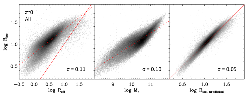
Figure 1: Relationship between the isophotal radius (in kpc) and (a) the effective radius (also in kpc), (b) the stellar mass (in Solar masses), and (c) a combination of the isophotal size and stellar mass that minimizes the scatter (from left to right). Isophotal size is poorly correlated with either the effective size or the stellar mass, but is tightly correlated with the linear combination of the two (in logarithm), providing a way to precisely predict isophotal radius if it is not available (see Eq. 6). Standard deviations of the residuals around the best linear fit (dashed line) are given in the panels. Solid lines show 1:1 relation where applicable. All of the low-redshift samples in this and subsequent figures come from GALEX-SDSS-WISE Legacy Catalog (GSWLC-M2).

Effective radii and Sérsic indices for the GOODS-S CANDELS high-redshift sample are taken from van der Wel et al. (2012), and were also derived using GALFIT. We use the effective radii and Sérsic indices estimated from the $H$-band (F160W) imaging, which is roughly comparable to to $r$ band at $z\sim 0$. We use the isophotal area from the Guo et al. (2013) photometric catalog ISOAREAF, also based on F160W, to which we apply a redshift and a zero-point corrections (Section 2.5).

Visual morphological classification into Hubble types is taken from the catalog of Nair & Abraham (2010), based on SDSS images. The redshift coverage of the catalog is the same as of our principal sample ($0.01<z<0.10$), but it contains far fewer objects (14 k) because it targets brighter galaxies ($g<16$), and is based on DR4, which has 60% of the area of DR7. We also utilize the sample of 3 k merger pairs from (Darg et al., 2010), identified based on the Galaxy Zoo visual classification of SDSS DR6 images (85% of DR7 area). The parent sample for this catalog has essentially the same redshift and magnitude selections as our primary sample.

Emission-line data needed for the selection of low redshift main sequence galaxies come from the MPA/JHU processing of SDSS DR7 spectra, which follows the methodology of Tremonti et al. (2004). We verify some of our results using the MPA/JHU SFRs and stellar masses, which were derived following the approach of Brinchmann et al. (2004).

2.4 SFR Surface Density ($\Sigma_{\mathrm{SFR}}$)

SFR surface density is defined as:

$$\Sigma_{\mathrm{SFR}}=\mathrm{SFR}/A$$ (1)

where $A$ is the physical (not the projected) area of a galaxy. In the case of an effective radius, the area is taken to be:

$$A=2R_{{\mathrm{eff},a}}^{2}\pi$$ (2)

where $R_{{\mathrm{eff},a}}$ corresponds to the semi-major axis ($a$) of the ellipse containing $1/2$ of the galaxy light, and the factor of two is meant to qualitatively take into account that the effective radius includes half of the galaxy light. Note that many studies, including Meert et al. (2015) that we use here, define effective radius as the geometric mean of the semi-major ($a$) and semi-minor ($b$) axes, the so called circularized effective radius ($R_{\mathrm{eff}}$). In that case $R_{\mathrm{eff}}^{2}\pi$ is not the physical area but the projected area ($ab\pi$), and we can introduce the projection factor ($f_{\mathrm{proj}}$) to go from the projected to the physical area:

$$A=2f_{\mathrm{proj}}\ R_{\mathrm{eff}}^{2}\pi$$ (3)

We determine $f_{\mathrm{proj}}$ empirically for the SDSS sample to be 1.26 (0.1 dex).

Similarly, for $\Sigma_{\mathrm{SFR}}$ based on the isophotal ellipse we use:

$$A=f_{\mathrm{proj}}\,R_{\mathrm{iso}}^{2}\pi$$ (4)

where the (circularized) isophotal radius ($R_{\mathrm{iso}}$) is the geometric mean of the apparent isophotal major and minor axes (given as isoA and isoB in SDSS DR7) and converted from angular to physical size using scale $s(z)$:

$$R_{\mathrm{iso}}=0.5s(z)\sqrt{{\tt isoA}\,{\tt isoB}}$$ (5)

The rationale for using the circularized sizes is that the linear extent ($a$) is less robustly constrained than $\sqrt{ab}$.

For galaxies without well-defined disks, such as the irregular galaxies and post-mergers, the isophotal ellipse may not be the most accurate way to establish the area. In such cases one can obtain the area as the sum of the area of the pixels that lie above some surface brightness threshold. Photometry software SExtractor (Bertin & Arnouts, 1996) provides such measurement as ISOAREAF and ISOAREA. This area should replace $R_{\mathrm{iso}}^{2}\pi$ in Equation 5.

2.5 Obtaining isophotal size from effective size and stellar mass

As we will show, $\Sigma_{\mathrm{SFR}}$is a more precise indicator of SF activity if derived using the isophotal size (or area), rather than the effective (half-light) size (Section 4.1). However, the isophotal size or area is often not reported in photometric catalogs. Or, if it is, it may be based on different thresholds. To overcome these practical issues, we devise a transformation from effective to isophotal radius, which we calibrate using our low-redshift, SDSS sample, and validate using CANDELS $0.8<z<2.5$ data.

The left panel of Figure 1 shows that the correlation between isophotal and effective physical radii is strongly non-linear and has a non-uniform scatter, suggesting that a direct conversion from effective to isophotal radii would be neither accurate nor precise. Fortunately, there is a way to improve the matters using the stellar mass. The middle panel of Figure 1 shows that the isophotal radius is also correlated with the stellar mass, though not much better than with respect to the effective radius, with the formal scatter around the best fit being similar—0.10 vs. 0.11 dex. However, it turns out that the $R_{\mathrm{iso}}$ is very well correlated with the combination of the effective radius and stellar mass, and with a scatter of just 0.05 dex:

$$\log R_{\mathrm{iso}}=0.188\log M_{*}+0.333\log R_{\mathrm{eff}}-1.037,$$ (6)

where sizes are in kpc and the stellar mass is in units of Solar mass. Isophotal size corresponds to 25 mag AB in $r$. The coefficients in Equation 6 were determined from a linear regression. In other words, stellar mass, isophotal radius and effective radius form a relatively tight 3D plane that contains both early and late type galaxies. The right panel of Figure 1 shows $R_{\mathrm{iso}}$ predicted from this relation to be reasonably unbiased. We tested expanding the calibration to include additional parameters (the Sérsic index or SFR), but further gains were very small ($\lesssim$2% reduction in scatter).

We expect the observed isophotal size to be affected by the cosmological surface brightness dimming. Indeed, when applying Equation 6 to CANDELS, we find the difference between the predicted and observed isophotal radii to be strongly redshift dependent. This allows us to construct a relation to use to correct the observed isophotal size of a galaxy at redshift $z$ to its value at $z\sim 0$:

$$\log R_{\mathrm{iso}}=\log R_{\mathrm{iso}}^{\mathrm{obs}}+0.129\,z$$ (7)

Note that the relation has not been tested at $z>2.5$.

Finally, we check the validity of our calibration for higher redshifts by comparing the predictions from Equation 6 to the actual, redshift-corrected isophotal sizes in CANDELS ($0.8<z<2.5$). The scatter between real and predicted sizes is 0.09 dex, in contrast to 0.17 dex between the isophotal and effective radii. Comparison reveals a small zero point offset (0.033 dex), arising from different surface brightness thresholds used in SDSS and CANDELS.

One potential concern is that some of the reduction in scatter in the $\Sigma_{\mathrm{SFR}}$ main sequence when using isophotal sizes derived from Equation 6 compared to effective sizes could be the product of the covariances introduced by the calibration itself. To test this, we compare the width of the SDSS $\Sigma_{\mathrm{SFR}}$ main sequence when using the isophotal sizes derived from Equation 6 and using the real $\Sigma_{\mathrm{SFR}}$. The latter is smaller (0.31 dex vs. 0.28 dex), suggesting that covariances do not affect it.

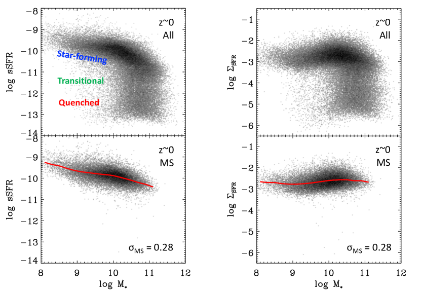
Figure 2: Low-redshift galaxy samples shown on the sSFR–$M_{*}$ (left) and $\Sigma_{\mathrm{SFR}}$—$M_{*}$ diagrams (right). Lower panels in both figures show the subset of galaxies that form the main sequence. The character of the main sequence changes when going from sSFR to $\Sigma_{\mathrm{SFR}}$ — it becomes more flat, while remaining tight (width, in dex, given in panels). Once the measure of SF activity is decoupled from the past SF history by using $\Sigma_{\mathrm{SFR}}$, the SF level is not strongly mass dependent.

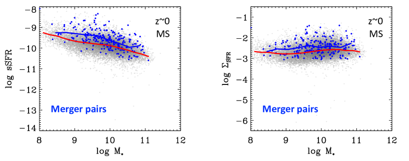
Figure 3: Main-sequence merger pairs (interacting galaxies) over-plotted on the general low-redshift main sequence population. Same galaxies are shown on the sSFR–$M_{*}$ (left) and $\Sigma_{\mathrm{SFR}}$—$M_{*}$ diagrams (right). Merger pairs serve as proxies for starbursts and come from Darg et al. (2010). Merging galaxies have a similar average offset (blue line) from the ridge of the overall main sequence (red line) in both cases; however, because there is no mass dependence, selecting starbursts by SFR surface density is obviously much cleaner than based on sSFR.

3 Results

In this section we explore, via sSFR–$M_{*}$ and $\Sigma_{\mathrm{SFR}}$–$M_{*}$ diagrams, the differences between sSFR and $\Sigma_{\mathrm{SFR}}$ as indicators of the degree of SF activity or quiescence. The analysis first focuses on the low-redshift sample and its various subsamples before turning to higher redshifts and the comparison to low redshift.

3.1 Low-redshift main sequence

The left panels of Figure 2 show the sSFR–$M_{*}$ diagram for the low-redshift sample. The upper panel contains all the galaxies in the sample, spanning 3.5 dex in stellar mass ($8<\log M_{*}<11.5$) and some 5 dex in sSFR ($-13.5<\log\mathrm{sSFR}<-8.5$). Higher-mass star-forming galaxies tend not to reach sSFR values that are as high as sSFRs of low-mass galaxies. This tilt of the main sequence can be seen more clearly in the lower left panel, which shows only the galaxies selected as star-forming in the BPT diagram. The tilt in the sSFR–$M_{*}$ main sequence, i.e., that $\alpha<1$ in SFR $\propto M_{*}^{\alpha}$, is a robust feature that exists irrespective of the choice of SFR indicator (Appendix A).

As discussed in Section 1, the tilt of the main sequence is an indication of mass-dependent SF histories and not of any change that would suggest quenching (a downward departure from an overall trend in SF history). However, an actual quenching would also lower sSFR, introducing an ambiguity in interpretation of a sSFR. $\Sigma_{\mathrm{SFR}}$ does not have this ambiguity and it should tell us about the current level of SF activity. Therefore, we now take a look at the lower panels of Figure 2, allowing us to contrast the appearance of the main sequence in sSFR–$M_{*}$ and in $\Sigma_{\mathrm{SFR}}$—$M_{*}$ diagrams. The two panels span the same dynamic range (6 dex) in the $y$ direction. The surface area used to normalize the SFR is based on isophotal sizes. This choice will be discussed in Section 4.1. Most notably, we see that the main sequence no longer has a downward tilt, and is quite flat (standard deviation of the mass-binned averages of $\Sigma_{\mathrm{SFR}}$ is 0.07 dex and the maximum amplitude of binned averages is 0.21 dex). There are possible breaks at $\log M_{*}=9.0$ and 10.4, which, by the way, are not at the same exact masses as the breaks in the sSFR–$M_{*}$ main sequence ($\log M_{*}=9.1$ and 10.0). These subtle features aside, the first conclusion we draw in this study is that the SF level of the present-day star-forming galaxies is remarkably constant across the stellar mass.

The defining feature of the sSFR–$M_{*}$ (or, equivalently, SFR–$M_{*}$) main sequence is that it is relatively tight. We find the width of both the $\Sigma_{\mathrm{SFR}}$—$M_{*}$ and the sSFR–$M_{*}$ main sequence to be the same (average of standard deviations in mass bins is 0.28 dex). This is despite the fact that the measurement error of $\Sigma_{\mathrm{SFR}}$ must be greater than on sSFR because it includes the error on galaxy size.

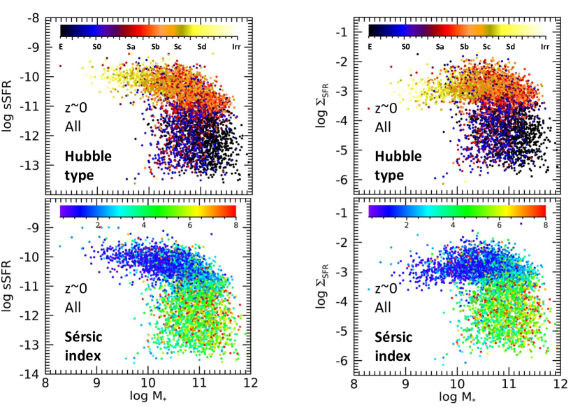
Figure 4: Subsample of low-redshift galaxies with Hubble types from Nair & Abraham (2010), shown on the sSFR–$M_{*}$ (left) and $\Sigma_{\mathrm{SFR}}$—$M_{*}$ diagrams (right). Upper panels are color-coded by the Hubble type, and lower panels by the Sérsic index (from Meert et al. 2015). Galaxies on the main sequence are mostly later types and have smaller Sérsic indices. SFR surface density provides a cleaner demarcation between early and late types than sSFR.

3.2 Low-redshift starbursts

Next we explore how well does $\Sigma_{\mathrm{SFR}}$ identify starburst galaxies compared to sSFR. To answer this, we need a sample of starbursts that is not identified using any SFR-related measure, because such reasoning would obviously be circular. That includes selecting by the the birth parameter $b=\mathrm{SFR}/$<SFR>, which is equivalent to an sSFR selection for a fixed galaxy age. Instead, here we utilize the fact that galaxy interactions can lead to an enhancement of SF and therefore such galaxies are more likely to be starbursting (e.g., Barton et al. 2000; Patton et al. 2013).

In Figure 3 we overplot on the general main-sequence sample the subsample of such galaxies identified visually in Darg et al. (2010) as merging pairs. We include all pairs regardless of the merging stage (separated, interacting, and approaching post-merger). The great majority of this sample are identified as being in the interacting stage. The left panel shows the sSFR–$M_{*}$ diagram. We see that the merging galaxies are indeed offset from the main sequence, with the mass-binned average difference of 0.29 dex (a factor of 2.0 enhancement, the same as found in Osborne et al. 2020 for galaxies out to $z\sim 2$, and in Patton et al. 2013 for pair separations $<30$ kpc). The plot shows that what makes a starburst is the relative enhancement in SF—selecting starbursts on some fixed sSFR value is clearly not justified. The offset between the interacting galaxy main sequence and the overall main sequence is not strongly mass dependent. From this it is immediately clear why the relative (s)SFR provides a much more meaningful way to select starbursts than any sSFR cut. The width of the interacting galaxy main sequence (0.36 dex) is not much larger than of the general main sequence (0.28 dex), suggesting a relatively uniform degree of SFR enhancement, having a standard deviation of 0.22 dex. Note that this standard deviation of SFR enhancement is likely partially suppressed by the SFR averaging timescale that our measure of SFR employs ($\sim$ 100 Myr) being longer than the starburst timescale ($\sim$50 Myr, Wuyts et al. 2009; Tacchella et al. 2020).

Turning the attention to the right panel of Figure 3, we see that the $\Sigma_{\mathrm{SFR}}$ main sequence of interacting galaxies is flat, and that it shows a similar offset with respect to the general main sequence, with the mass-binned average difference of 0.21 dex (a 60% enhancement). The width of the interacting galaxy $\Sigma_{\mathrm{SFR}}$main sequence is even more similar to the overall $\Sigma_{\mathrm{SFR}}$ main sequence (0.32 dex vs. 0.28 dex), implying a standard deviation of the enhancement in $\Sigma_{\mathrm{SFR}}$ of just 0.13 dex. From the flatness of interacting galaxy $\Sigma_{\mathrm{SFR}}$ main sequence we conclude that a selectivity of $\Sigma_{\mathrm{SFR}}$ to starbursts must be at least as good as using the relative SFR. We confirm this more directly by comparing $\log\mathrm{(sSFR/sSFR_{MS})}$ to log $\Sigma_{\mathrm{SFR}}$, and finding that Darg et al. (2010) star-forming mergers form an even sharper lower boundary in SFR surface density (at log $\Sigma_{\mathrm{SFR}}$ $=-3.0$) than in the relative SFR. Selection of starbursts using a threshold in $\Sigma_{\mathrm{SFR}}$ is not a new thing (Kennicutt & Evans, 2012), but its preference to other methods has not been universally recognized.

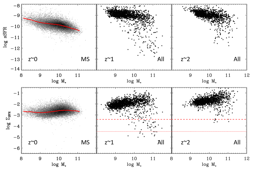
Figure 5: Evolution of galaxies in sSFR–$M_{*}$ (upper panels) and $\Sigma_{\mathrm{SFR}}$—$M_{*}$ diagrams (lower panels). For low-redshift samples we show only the main-sequence galaxies. In sSFR–$M_{*}$ diagrams the slope of the main sequence stays more or less the same, whereas $\Sigma_{\mathrm{SFR}}$—$M_{*}$ diagrams reveal a change—there was a higher SF activity of massive galaxies compared to less massive ones in the past, consistent with a bulge build-up of those systems. Dashed line in lower panels signifies the upper boundary of the low-redshift transition region. At higher redshift this boundary is higher and would have encompassed today’s main sequence galaxies. The dotted line represents the threshold for full quenching, which is independent of the redshift.

3.3 Low-redshift transitional/quenched galaxies

Before becoming fully quenched, the galaxies must transition, so that their sSFRs are significantly lower than on the main sequence, but are not yet entirely devoid of SF. It should be noted that observationally establishing a complete absence of SF is challenging. Although not formally having a SFR of zero (which the SF history parameterization used in the SED fitting does not even allow), the galaxies with log sSFR $<-12$ typically show no evidence of star-forming regions in UV images and can be considered as fully quenched for all practical purposes.

We next ask how well does $\Sigma_{\mathrm{SFR}}$ separate the actively star-forming galaxies from the ones that have or are experiencing quenching, i.e., the transitional galaxies. As in the case of starbursts, we cannot define the quenching galaxies using any of the measures that we wish to evaluate (sSFR, relative SFR and $\Sigma_{\mathrm{SFR}}$). Instead, we will take advantage of the fact that the transitional/quenching galaxies, unlike the ones that are not quenched, all have prominent spheroidal components. Qualitatively, this means that we expect the transitional galaxies to be dominated by early-type galaxies (ellipticals, lenticulars and early-type spirals). Quantitatively, we expect the profiles of the galaxies to be more highly concentrated, as reflected in their Sérsic indices being higher.

In Figure 4 we again show sSFR–$M_{*}$ (left panels) and $\Sigma_{\mathrm{SFR}}$—$M_{*}$ diagrams (right panels) of galaxies matched to Nair & Abraham (2010) catalog and color code them by the Hubble types provided in that catalog (upper panels), and by the Sérsic indices from Meert et al. (2015) (lower panels). A clear trend is present on the sSFR–$M_{*}$ plots—the main sequence is dominated by late-type spirals (Sd at $\log M_{*}<9.8$, Sc and Sb types above that mass), whereas the region below the main sequence is dominated by ellipticals and S0s, with the former being more dominant at higher mass. Interestingly, the main-sequence spirals can be as massive as any but the most massive of the early-type galaxies. A trend similar to that with the Hubble type is seen with respect to the Sérsic index, where we see a significant increase in a typical Sérsic index starting just below the main sequence. Note, however, that at any point in the sSFR–$M_{*}$ plane there exists a range of Sérsic indices and Hubble types, i.e., the trends are there, but are not very tight. This confirms the finding of Wuyts et al. (2011) that the galaxies are not just a two-parameter (SFR, $M_{*}$) family.

We can see that the “threshold” for the morphological transition in sSFR–$M_{*}$ is somewhat tilted, following the tilt of the main sequence. This suggests that, as in the case of starbursts, it is the relative SFR that provides a cleaner morphological distinction than sSFR, as previously pointed out by Wuyts et al. (2011). On the other hand, in $\Sigma_{\mathrm{SFR}}$—$M_{*}$ (Figure 4, upper right panel) the transition in Hubble types is essentially flat, i.e., it happens at a fixed $\Sigma_{\mathrm{SFR}}$. This transition in $\Sigma_{\mathrm{SFR}}$ is as sharp as it is for the relative SFR. We confirm this quantitatively by determining the interval over which the fraction of early-type galaxies ($T\leq 0$) increase from the level typical for the main sequence (12%) to the level typical among the quiescent galaxies (93%). This interval is 1.0 dex for both log $\Sigma_{\mathrm{SFR}}$ and $\log\mathrm{(sSFR/sSFR_{MS})}$, compared to 1.2 dex for log sSFR. We also fitted a logistic function to the fraction of ETGs vs. the parameter, and the slope is steepest with respect to $\Sigma_{\mathrm{SFR}}$. Similar results are found regarding how sharply the fraction of galaxies with high Sérsic index ($n>2.5$, corresponding to classical bulges, Drory & Fisher 2007) rises as a function of decreasing sSFR, relative SFR, or $\Sigma_{\mathrm{SFR}}$. To conclude, $\Sigma_{\mathrm{SFR}}$ produces a cleaner separation between late and early-type galaxies than sSFR, and is as clean as the relative SFR.

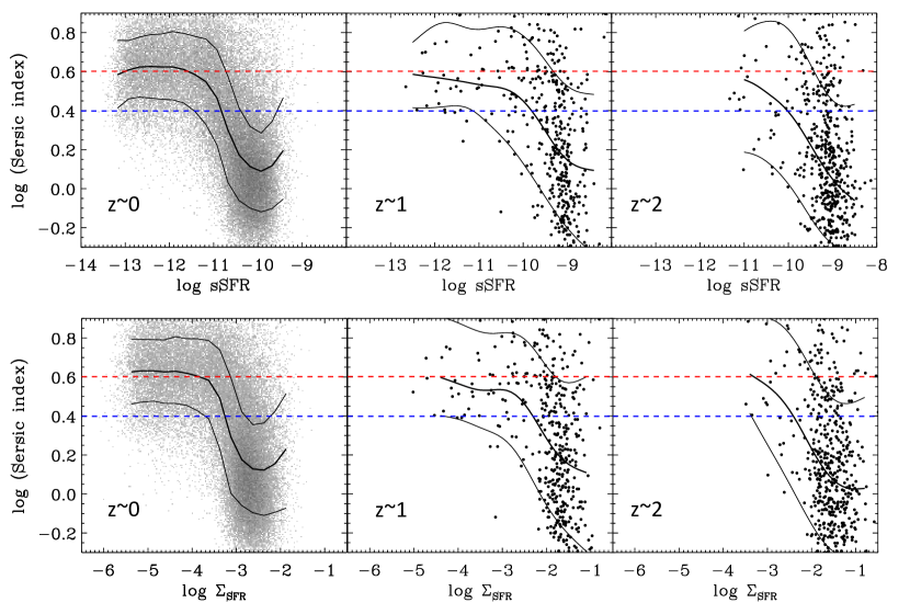
Figure 6: Trends of the Sérsic index as a function of sSFR (upper panels) and $\Sigma_{\mathrm{SFR}}$ (lower panels), at different redshifts. The galaxies with today’s values of sSFR or $\Sigma_{\mathrm{SFR}}$ characteristic of the main sequence would be found below the main sequence at high redshift, and like the transiting galaxies today, would have, on average, a high Sérsic index. This suggests that morphological transformation is associated with a relative suppression of sSFR or $\Sigma_{\mathrm{SFR}}$, but to values which would still be considered quite high for today’s norms. The red dashed line corresponds to $n=4$ de Vaucouleurs’ profile, and the red line corresponds to $n=2.5$, an approximate dividing line between the galaxies with and without a central spheroid. Shown are the galaxies with $10<\log M_{*}<11$. Curves represent the 16 percentile, the mean, and the 84 percentile in each $x$-axis bin. Curves at $z\sim 1$ and $\sim 2$ are smoothed to mitigate low numbers of objects.

3.4 High-redshift main sequence

Our attention is now turned to higher redshift samples and the evolution between $z\sim 2$ and $z\sim 0$. In the upper panels of Figure 5 we are showing the sSFR-$M_{*}$ diagrams at $z\sim 0$, 1 and 2. We see that the fraction of high-redshift ($z\sim 1$ and 2) galaxies below the main sequence is much smaller than in SDSS, so for clearer comparison we only show the main-sequence sample for low redshift. We first note that there is not much evolution in sSFR-$M_{*}$ between $z\sim 2$ and $z\sim 1$—the slope and the normalization of the main sequence are similar. Actually, the slope of the main sequence is not very different at low redshift either ($-0.34$ at $z\sim 0$ compared to $-0.27$ at $z\sim 1$ over the same mass range, $9<\log M_{*}<11$), as noted already in Noeske et al. (2007). However, as expected, the normalization today is significantly lower—0.9 dex with respect to $z\sim 1$. So, based on the invariant slopes of the main sequence in sSFR (or, alternatively, just SFR) one might conclude that SF is less active at all masses by a similar degree.

The picture looks different with $\Sigma_{\mathrm{SFR}}$ replacing sSFR (lower panels of Figure 5). Again, there seems to be little evolution between $z\sim 2$ and $z\sim 1$ in terms of the slope and the normalization of the $\Sigma_{\mathrm{SFR}}$ main sequence. However, unlike the case of sSFR-$M_{*}$, we see a change between low and high redshift, not only in the normalization, but also in the slope of the main sequence. The slope is slightly positive at $z\sim 0$ (slope 0.11), whereas it is 0.25 at $z\sim 1$. So, based on the main sequence in $\Sigma_{\mathrm{SFR}}$ we conclude that the level of SF activity since the “cosmic noon” has dropped more for massive galaxies ($9\times$ for $10.6<\log M_{*}<11.0$) than for low-mass ones ($5\times$ for $9.0<\log M_{*}<9.4$).

3.5 High-redshift transitional/quenched galaxies

Here we address a question: can the distinction between a non-quenched and a transitional galaxy be based on a redshift-invariant parameter? We know that sSFR does not provide this, because the normalization of the main sequence changes, and the lower panels of Figure 5 show that neither does $\Sigma_{\mathrm{SFR}}$—the $\Sigma_{\mathrm{SFR}}$ main sequence also changes in redshift, as discussed in the preceding section. In other words, at a given stellar mass a typical high-redshift galaxy will have both the higher SFR and the higher SFR per surface area compared to a present-day galaxy.

To further explore if it is justified to consider a galaxy with the same $M_{*}$ and the same SFR (or $\Sigma_{\mathrm{SFR}}$) as quenching at one redshift and not quenching at another, we again look at the structural properties. Figure 6 presents, for the same three redshift bins, the Sérsic index as a function of sSFR (upper panels) and $\Sigma_{\mathrm{SFR}}$ (lower panels). At $z\sim 0$, the average Sérsic index for a galaxy at log sSFR $=-10.2$ (main sequence at that redshift) is $n=1.3$—an exponential disk. On the other hand, the average Sérsic index at that same sSFR at $z\sim 1$ is $n=3.0$, typical of early-type galaxies today. A similar result is obtained if considering $\Sigma_{\mathrm{SFR}}$. From this we confirm the Wuyts et al. (2011) conclusion that the transitional/quenching status is indicated by the SFR (or in our case also $\Sigma_{\mathrm{SFR}}$) relative to the main sequence at that redshift, and not by any absolute threshold in either sSFR or $\Sigma_{\mathrm{SFR}}$.

Whereas the criterion for the onset of quenching remains tied to the position with respect to the main sequence for either the (s)SFR or $\Sigma_{\mathrm{SFR}}$ main sequence, the achievement of full quiescence is still meaningful as a fixed, redshift-independent threshold in $\Sigma_{\mathrm{SFR}}$, but not in sSFR or relative SFR. The reason for this is again that unlike sSFR, $\Sigma_{\mathrm{SFR}}$ is not the young-to-old population contrast, but an absolute measure of the young population. Similar ambiguity regarding the threshold for full quiescence would apply to a color, or H$\alpha$ equivalent width, as both are contrasting the young and old population. Locally, the bottom boundary of the transitional region appears to be around log $\Sigma_{\mathrm{SFR}}$ $=-4.5$. Establishing the lowest $\Sigma_{\mathrm{SFR}}$ for transitional galaxies is difficult because of the difficulties involved with measuring very low levels of SF, so we consider this threshold as provisional. If we take this threshold to be redshift independent, Figure 5 shows that very few galaxies at $z\sim 1$ and no galaxy at $z\sim 2$ fall below it. It should be noted however that constraining these low $\Sigma_{\mathrm{SFR}}$ values, especially at high redshift is challenging and sensitive to the assumptions regarding the SF histories used in the SED fitting, so it is difficult to know for sure if any of them fall below the log $\Sigma_{\mathrm{SFR}}$ $=-4.5$ threshold.

We should also point out that the $\Sigma_{\mathrm{SFR}}$ radial profiles of galaxies typically decline towards the outskirts (e.g., Gil de Paz et al. 2007), which means that any threshold that we want to attach to full quiescence will depend on the size used for $\Sigma_{\mathrm{SFR}}$. If we were to use the effective radii instead of isophotal, the proposed threshold for quiescence would be $\sim$1 dex higher (log $\Sigma_{\mathrm{SFR}}$ $=-3.5$). Similarly, the $\Sigma_{\mathrm{SFR}}$ defining the lower envelope of the main sequence (the threshold for the onset of transitional region) will de different depending on the size of the aperture used to obtain $\Sigma_{\mathrm{SFR}}$.

There are several additional things one can infer from Figure 6.

1. At all redshifts, galaxies with high Sérsic indices are common on the main sequence, but the reverse is not true—there are few low-$n$ transitional/quenched galaxies. Indeed the lower threshold for Sérsic index off the nain sequence ($n\approx 2.5$) coincides with the demarcation between the galaxies containing the central spheroid (classical bulge) and the ones that do not (Drory & Fisher, 2007). This confirms previous results regarding the structure of quenching or quenched galaxies (Bell, 2008; Mosleh et al., 2017) and that the compaction starts on the main sequence (Cheung et al., 2012; Barro et al., 2017).

2. The low-redshift sample shows that the galaxies above the main sequence are on average more compact (1.25 times higher $n$) than on the main sequence. A similar trend has been reported in Schiminovich et al. (2007); Wuyts et al. (2011), and is consistent with a compaction proceeding via a starburst stage (Schiminovich et al., 2007; Tacchella et al., 2016; Lapiner et al., 2023).

3. The transitional region has a similar 68 percentile range of Sérsic indices as the the main sequence or the quiescent region, i.e., it is inconsistent with being the mix of the tails of two populations, as such mixing would widen the distribution in the transitional region.

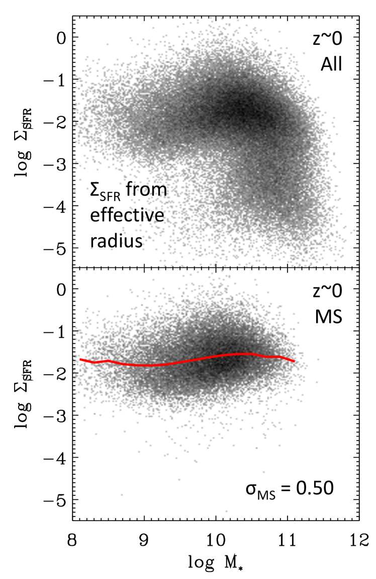
Figure 7: The effects on the $\Sigma_{\mathrm{SFR}}$—$M_{*}$ relation arising from defining the SFR surface density using the effective (half-light) radius. This figure is to be compared to the right panel of Figure 2, which uses the isophotal sizes, our nominal choice. Effective radius-based $\Sigma_{\mathrm{SFR}}$ are significantly noisier, leading to a broader main sequence (width, in dex, given in lower panel). The effective radius, being dependent on the galaxy light profile, is not as good of an indicator of the extent over which SF is (or was) taking place as is the isophotal radius.

4 Discussion

4.1 Relevant measure of galaxy size for $\Sigma_{\mathrm{SFR}}$

It is common in the literature to obtain the global SFR surface density either using the effective (half-light) radius, or using the isophotal radius. We have found that the choice of measure is very important. In Figure 7 we show the $\Sigma_{\mathrm{SFR}}$—$M_{*}$ diagram for our low-redshift samples in which $\Sigma_{\mathrm{SFR}}$ is based on the effective radius (Eq. 3). This figure is to be compared to the right panel of Figure 2, which was based on the isophotal radius (Eq. 4). As expected, the absolute values of $\Sigma_{\mathrm{SFR}}$ are higher, because the isophotal sizes are about three times larger on average than the effective one (Figure 1). Nonetheless, the relatively flat shape (and even the details of the inflections) of the $\Sigma_{\mathrm{SFR}}$ main sequence remain.

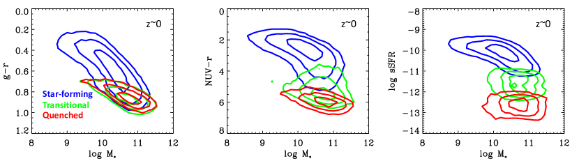
Figure 8: The placement of galaxies separated into star-forming, transitional and quenched (quiescent) categories on various diagrams with stellar mass on the $x$ axis. Panels from left to right demonstrate the successive improvements in the ability to separate these categories afforded by moving from optical to UV-optical color and then to sSFR. Specific SFRs provide a good separation between these categories, but the use of $\Sigma_{\mathrm{SFR}}$ (based on which these categories have been defined) goes an additional step by eliminating the effect of age on the main sequence (its tilt).

What has drastically changed is the the width of the $\Sigma_{\mathrm{SFR}}$ main sequence. Its scatter around the mean is 0.50 dex, compared to 0.28 dex for the main sequence based on the isophotal radius. Furthermore, $\Sigma_{\mathrm{SFR}}$ based on the effective radius is less well able to distinguish between the early and late type galaxies. Overall, it is a much noisier measure of the level of SF activity than the $\Sigma_{\mathrm{SFR}}$ based on the isophotal radius. This worse performance cannot be due to the differences in the precision of the measurements of two sizes. If anything, the measurements of the effective size are more robust than the isophotal one (Trujillo et al., 2020; Chamba, 2020). Effective radii used in this exercise are from the Meert et al. (2015) catalog. An alternative source of SDSS effective sizes, the catalog of Simard et al. (2011), yields similar results (main sequence scatter of 0.48 dex). Looking at yet other measures of galaxy size, both Meert et al. (2015) and Simard et al. (2011) catalogs provide estimates for the scale lengths of the disk components alone. However, $\Sigma_{\mathrm{SFR}}$ based on these disk scale lengths (which are proportional to disk effective radii) produce small or no improvement in terms of the main sequence scatter compared to the effective radii of full galaxies.

We propose that the fundamental reason why isophotal sizes produce more meaningful $\Sigma_{\mathrm{SFR}}$ lies in the fact that they better reflect the extent over which the star formation is taking place. Isophotal and effective size are actually very different measures. To first order the isophote reflects a certain mass density threshold, and is therefore related to the extent over which SF happens. On the other hand, the effective radius is sensitive to the galaxy profile, i.e., its structure. This can be illustrated by the following example. Take two identical bulge-less disk galaxies. Their isophotal areas are the same. Now let us place in one of them a massive compact bulge with no ongoing star formation. The effective radius of that galaxy shrinks, leading to a higher $\Sigma_{\mathrm{SFR}}$ if it was based on the effective size, even though nothing has changed in terms of the extent over which SF takes place. The isophotal size and $\Sigma_{\mathrm{SFR}}$ based on it however, are not affected by this addition of a bulge.

Recently, Trujillo et al. (2020) have argued against the effective size, on the grounds that it depends on the light profile, and illustrate their point with an example similar to one above. Instead, they have proposed an “iso-mass” measure of size based on the mass density threshold of 1 $M_{\odot}\mathrm{kpc}^{-2}$. Isophotal sizes are a good proxy for iso-mass sizes, as confirmed by Tang et al. (2020), who found that the optical colors of different galaxies at 25 AB mag arcsec^-2 in $g$-band are quite uniform, implying, via color—$M/L$ relation, that such isophote is a good tracer of stellar mass surface density. Our nominal isophotal size is based on 25 AB mag arcsec^-2 in $r$-band, which is somewhat deeper than the traditional 25 Vega mag arcsec^-2 in $B$-band. We find that the isophotal sizes based on $u$ and $g$-band produce almost identical results as $r$ in terms of the width of the main sequence and the ability to distinguish early-type galaxies, even though they correspond to somewhat smaller (0.22 dex and 0.06 dex, respectively) physical sizes than the $r$-band isophote. Conceptually, it is not clear that one should aim to use the area based on the very short wavelengths. Tying the SFR surface density to an area over which a SF is or could be taking place (if gas was present), which is achieved by using optical sizes, allows us to incorporate both the actively star-forming and the quiescent galaxies (for which SFRs are essentially upper limits and UV sizes would be meaningless) into a single scheme.

We conclude that any sort of “iso” size (isophotal or iso-mass) will be more appropriate as a basis for $\Sigma_{\mathrm{SFR}}$ as an indicator of SF activity than an effective size. Indeed, the original global Kennicutt-Schmidt relation is based on the $\Sigma_{\mathrm{SFR}}$ from the isophotal size (Kennicutt, 1989; Buat et al., 1989), and the rationale for this choice given in Kennicutt (1998) was that the isophotal radius is comparable to the extent of active SF disk in H$\alpha$. For these and other reasons that suggest that isophotal sizes are better behaved and provide tighter scaling relations (e.g., Saintonge & Spekkens 2011; Tang et al. 2020), future surveys should aim to include them in their catalogs. If that is not possible (for example due to the difficulties arising from the cosmological dimming), a viable alternative would be to estimate the isophotal size from the combination of the effective size and the stellar mass (Section 2.4). Indeed, using this calibration to infer isophotal sizes essentially recovers the tightness of the $\Sigma_{\mathrm{SFR}}$ main sequence (0.30 dex, vs. 0.28 dex with the actual isophotal size).

4.2 Towards a more physical measure of SF activity

Being tied to the gas densities and the effectiveness of stellar feedback, the $\Sigma_{\mathrm{SFR}}$ may be considered as a move towards a more physical measure of the current SF activity/quiescence. In that sense, a switch to $\Sigma_{\mathrm{SFR}}$ aims to provide further conceptual and practical improvements, similar to one that sSFR had with respect to the use of optical color. As illustrated in the left panel of Figure 8, the optical color of actively star-forming galaxies is even more strongly affected by the age of stellar populations than sSFR, and produces a steep tilt when plotted against the mass. Furthermore, the optical color has very poor sensitivity to low relative levels of SF (e.g., Kauffmann et al. 2007), which results in an inability to distinguish between transitional and fully quenched galaxies (Salim, 2014). As a result, even the massive main-sequence galaxies have optical colors nearly as red as the early-type galaxies (Cortese, 2012), affecting the quenched fraction estimates based on optical color (Figure 8, left panel) and making it appear as if there were no, or very few, massive star-forming galaxies. UV-optical color overcome many of the limitations of the optical colors (middle panel of Figure 8), but is subject to dust and metallicity effects (which can somewhat be mitigated by combining UV-optical color with a optical-near-IR color, e.g., in NUV–$r$–$J$ diagram, Arnouts et al. 2013). sSFR determined from the SED fitting effectively utilizes a range of UV-optical-near-IR color, but being constrained using the models that include dust and metallicity effects, is not subject to them. As a result, it provides a cleaner separation between star-forming, transitional and quenched galaxies (Figure 8). Finally, $\Sigma_{\mathrm{SFR}}$ improves over sSFR by removing the age effect, which through $M_{*}$ or red optical band was present in all previous measures discussed here.

Kennicutt & Evans (2012) considered $\Sigma_{\mathrm{SFR}}$ as one of the two ways to normalize SFR, the other being the sSFR. They also commented that the range of $\Sigma_{\mathrm{SFR}}$ for normal (non-starburst) galaxies is relatively small and in that sense similar to the range of sSFR. More quantitatively, we see that the observed $\Sigma_{\mathrm{SFR}}$ main sequence has the same scatter as the sSFR main sequence (0.28 dex, Section 3.1), and intrinsically, the $\Sigma_{\mathrm{SFR}}$ main sequence may be even narrower than the sSFR one. Namely, since we measure the scatter in small mass bins, the only contributor to sSFR measurement uncertainty is that of SFR. On the other hand, $\Sigma_{\mathrm{SFR}}$ has measurement uncertainties from both the SFR and the isophotal area. This is an indication that $\Sigma_{\mathrm{SFR}}$ may be a more physical measure of current SF activity than sSFR.

Furthermore, replacing sSFR with $\Sigma_{\mathrm{SFR}}$ almost entirely removes the downward tilt of the main sequence at low redshift and even results in a slight upward trend (Figure 2). The downward tilt of the main sequence in sSFR–$M_{*}$ is essentially the result of SF histories being dependent on the mass, and is unrelated to the current SF level (see Section 1). On the other hand, the main sequence based on the SFR surface density makes the character of the ongoing SF more uniform for galaxies of different masses. The relative constancy of $\Sigma_{\mathrm{SFR}}$ across the main sequence was first pointed out by Schiminovich et al. (2007), who called the result “intriguing”. That result has not received much attention and, as far as we are aware, was not the focus of any theoretical work. We now find that at higher redshifts the $\Sigma_{\mathrm{SFR}}$ actually rises with the mass. This is consistent with the rapid growth of the central mass concentration (a bulge) in more massive galaxies, but less so in present-day dwarfs and late spirals. Slight upward tilt of the $\Sigma_{\mathrm{SFR}}$ main sequence at $z\sim 0$ may suggest that there is still some in-situ bulge build-up in massive star-forming galaxies. We agree with Schiminovich et al. (2007), who concluded that the redshift evolution lies fundamentally in $\Sigma_{\mathrm{SFR}}$. Indeed, a galaxy which maintains a constant SFR will be progressively dropping in sSFR by definition. Considering that $\Sigma_{\mathrm{SFR}}$ provides complimentary information to (s)SFR, we propose that $\Sigma_{\mathrm{SFR}}$—$M_{*}$ scaling relation be included among the benchmarks for galaxy simulations.

A flattening of the main sequence can to some degree be produced by normalizing SFR not by the total stellar mass, but only the disk stellar mass, as proposed and shown by Abramson et al. (2014). An underlying assumption behind this modification is that the bulge represents an inert component that is not associated with the current star formation. We confirm with our low-redshift sample that replacing the nominal sSFR with the disk-only sSFR, obtained by multiplying our total stellar mass with the disk-to-(disk+bulge) mass ratio from the $n=4+1$ decompositions of Mendel et al. (2014), reduces the tilt of the main sequence from $-0.35$ to $-0.20$ ($\log M_{*}>8$). The disk sSFR main sequence is broader than the nominal sSFR one (0.36 dex vs. 0.28 dex), most likely because of the greater uncertainties in deriving the stellar mass of the disk component compared to the total stellar mass. Disk-bulge decompositions are especially challenging based on SDSS images. By using the disk mass to normalize SFR, this measure becomes partially decoupled from the past SF history and therefore has similar aims as the use of $\Sigma_{\mathrm{SFR}}$. One conceptual advantage of $\Sigma_{\mathrm{SFR}}$ is that it allows purely spheroidal galaxies with no disk to be encompassed by the scheme.

Many studies nowadays use the relative SFR as a principal variable of the analysis. Relative SFR will by construction flatten the sSFR main sequence tilt. It was introduced by Schiminovich et al. (2007) for the very reason of eliminating the dependence of sSFR on $M_{*}$. There is no ambiguity that in the relative sense (for galaxies of fixed mass) the galaxies with the high relative SFR can be considered as experiencing a current burst, whereas the galaxies with low relative SFR have or are experiencing quenching and have a diminished current capacity to form stars. Our analysis shows that the relative SFR has a comparable ability to identify starbursts and early-type galaxies as does $\Sigma_{\mathrm{SFR}}$. Its non-optimal aspect is that it is defined relative to a main sequence that needs to be observationally established, which is by no means unambiguous, especially at the massive end where the main sequence blends with the turn off. More importantly, by referring to SFRs in relative terms, we are in a way giving up on the idea that there is a physical quantity that describes the SF level. Interestingly, Schiminovich et al. (2007) said that the physical basis for the introduction of the relative SFR comes from its correlation with $\Sigma_{\mathrm{SFR}}$.

Global (integrated) SFR surface density is not commonly considered in the studies of galaxy evolution outside of the context of the Kennicutt-Schmidt relation. For example, the SF history is usually defined as the change in SFR over time. Lehnert et al. (2014), on the other hand, discuss the evolution of the MW in terms of the change in $\Sigma_{\mathrm{SFR}}$ (which they call SF intensity, cf. Lanzetta et al. 2002; Boquien et al. 2010). They note that it is $\Sigma_{\mathrm{SFR}}$ that determines the role of stellar feedback on outflows and on mass–metallicity relation.

Likewise, $\Sigma_{\mathrm{SFR}}$–$M_{*}$ featuring global SFR density is a rarely used diagram. Kelly et al. (2014) and Lunnan et al. (2015) used it to compare SF properties of long gamma ray bursts and superluminous supernovae hosts to that of other supernova hosts (and find them to be elevated.) Tran et al. (2017) use it to compare field and cluster galaxies at $z\sim 2$, and describe $\Sigma_{\mathrm{SFR}}$ as the intensity of SF. Förster Schreiber et al. (2019) show the $\Sigma_{\mathrm{SFR}}$–$M_{*}$ diagram of 600 galaxies at $0.6<z<2.7$ color-coded by incidence of outflows. The incidence follows $\Sigma_{\mathrm{SFR}}$ remarkably well (as pointed out in Heckman 2002; Newman et al. 2012), and somewhat better than the main sequence offset (their Fig. 7). Interestingly, their $\Sigma_{\mathrm{SFR}}$–$M_{*}$ main sequence shows an upward tilt similar to what we saw in the $z\sim 1$ panel of Figure 5.

4.3 Implications for studies of resolved star formation

The advent of the integral field unit (IFU) spectrographs and associated surveys, such as MaNGA (Bundy et al., 2015), CALIFA (Sánchez et al., 2016) and SAMI (Bryant et al., 2015), has shifted the focus from general considerations of global SF level to trying to understand the processes of SF regulation on spatially resolved scales. The most common aspect of IFU studies concerns the radial profile of SF activity and the question of the dynamics of the quenching process, such as the inside-out vs. the outside-in scenarios (e.g., Tacchella et al. 2015; Belfiore et al. 2018; Lin et al. 2019).

One can imagine making two types of radial profiles that involve SFR-related quantities. One is the sSFR radial plot, where the SFR in a radial bin is divided by the stellar mass in that radial bin (sometimes designated as $\Sigma_{\mathrm{sSFR}}$), and another is the $\Sigma_{\mathrm{SFR}}$ radial plot, where the SFR is divided by the physical area of the radial bin. Here we wish to point out that the sSFR radial profile is subject to the same ambiguities as the global sSFR in the sense that sSFR depends on both the current SF level and the past SF history. Consider an example of a galaxy with a prominent bulge, i.e., a large stellar mass concentration. A profile of such a galaxy could likely be redder in the bulge area, corresponding to a dip in the sSFR profile. However, lower sSFR because of the substantial mass does not imply that SF levels are suppressed. SF may actually be present in the bulge at the same or higher levels than further out in the disk (Tacchella et al., 2018). There is no question that in such a case the current SF in the central region contributes relatively little to the stellar mass compared to when the bulge was being built up, but that relative change does not imply that any active quenching is taking place now, rather than just a gradual decline. Thus, for galaxies that have red (low sSFR) centers but significant amount of SF, the more neutral term may be the inside-out build-up (e.g.  Nelson et al. 2016; Lilly & Carollo 2016; Belfiore et al. 2018), rather than the inside-out quenching.

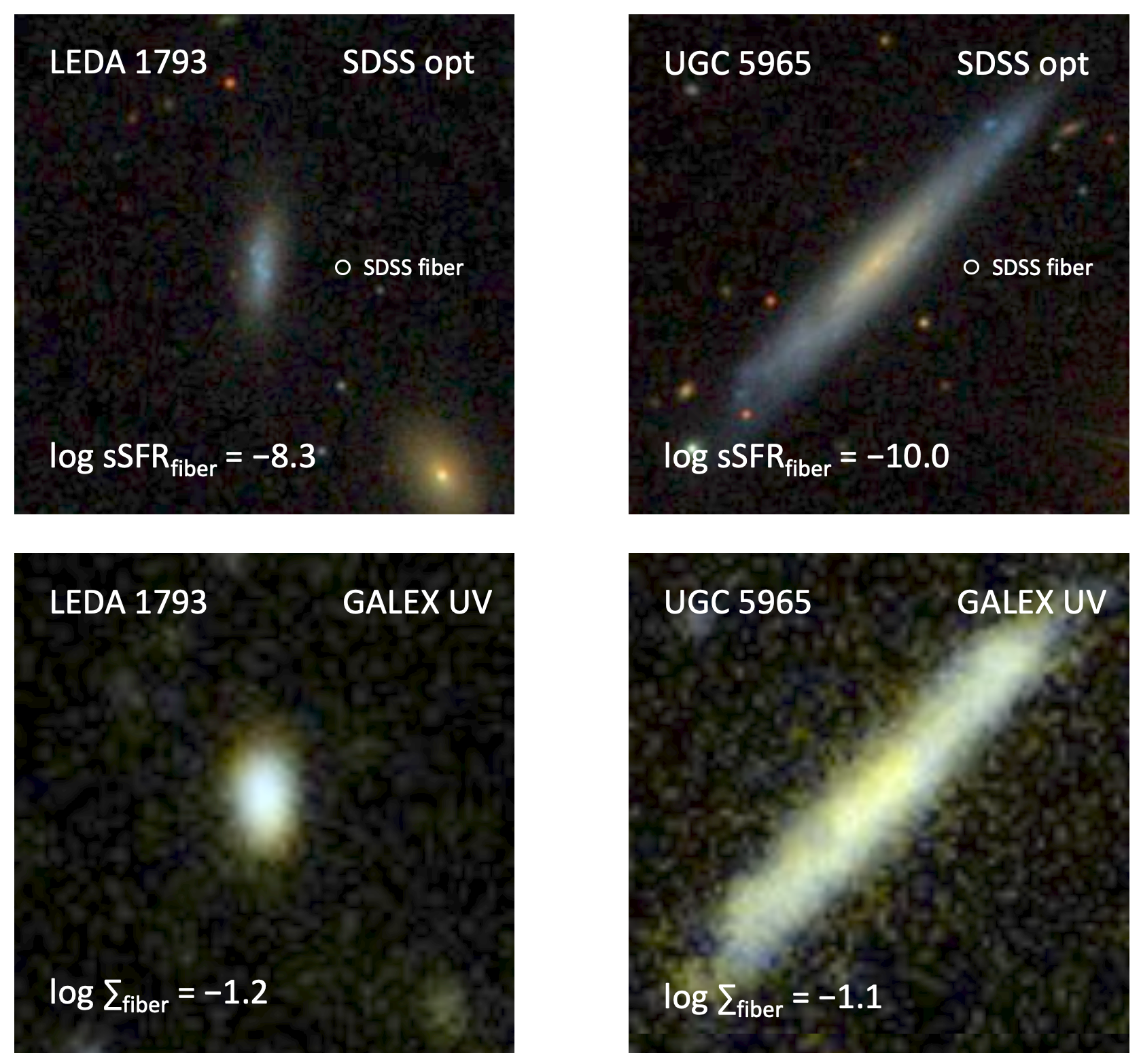
Figure 9: Differences in inferences regarding a galaxy’s star formation based on whether sSFR or $\Sigma_{\mathrm{SFR}}$ is considered. Left panels correspond to LEDA 1793, whereas right panels show UGC 5965. Upper panels present optical images from SDSS and the lower panels are UV images from GALEX. UGC 5965 has a red center, but its central SFR surface density is as high as that of LEDA 1793, which is blue and has a high central sSFR. Quantities are based on dust-corrected H$\alpha$ and correspond to 3 arcsec SDSS fiber, shown as a circle. SDSS images are taken from SkyServer, whereas GALEX images (far-UV plus near-UV composites) are from the Legacy Survey Sky Browser.

We illustrate this point with a specific example in Figure 9, where we take advantage of sSFR and $\Sigma_{\mathrm{SFR}}$ determined from dust corrected H$\alpha$ within the SDSS spectroscopic fiber to probe central quantities. Galaxy on the left (LEDA 1793) has a very high central sSFR, appearing as a blue compact dwarf, whereas sSFR is significantly lower for the galaxy on the right (UGC 5965). UGC 5965 has a distinctly red bulge in SDSS image. The UV images from GALEX paint a different picture. UGC 5965 reaches the highest UV brightness in the bulge. As a matter of fact, the UV surface brightness appears to be similar in UGC 5965 and LEDA 1793, as corroborated by nearly identical $\Sigma_{\mathrm{SFR}}$ in the fiber.

5 Conclusions

Replacing (s)SFR with $\Sigma_{\mathrm{SFR}}$ in the galaxy “HR diagram” has given us a different perspective regarding the character of SF on and off the main sequence, and its evolution. The main findings are:

1. The SFR surface density ($\Sigma_{\mathrm{SFR}}$) is largely insensitive to past SF history and thus provides a measure of the current global star-forming level of a galaxy tied to its molecular gas density. This is contrast to sSFR, a relative measure of young-to-old population.

2. $\Sigma_{\mathrm{SFR}}$ provides a cleaner separation of likely starbursts and spheroid-dominated (early-type) galaxies than sSFR. Its selection power is comparable to that of the SFR offset relative to the main sequence.

3. $\Sigma_{\mathrm{SFR}}$ of the main-sequence galaxies at low redshift is essentially mass-independent. Dwarfs and high-mass spiral (disk) galaxies have very similar levels of star-forming activity. This was first pointed out in Schiminovich et al. (2007).

4. $\Sigma_{\mathrm{SFR}}$–$M_{*}$ main sequence at $z\gtrsim 1$ is tilted upwards: high-mass galaxies had $\sim 2\times$ higher SF levels than lower-mass galaxies, possibly reflecting a rapid build up of a central mass concentration (bulge). Such trend is not seen in SFR–$M_{*}$ or sSFR–$M_{*}$ diagrams, the slope of which does not evolve much between $z=0$ and $z=2$. Because of this complementarity, we propose that $\Sigma_{\mathrm{SFR}}$—$M_{*}$scaling relation be included among the benchmarks for galaxy simulations.

5. We confirm that galaxies that fall below the main sequence at high redshift are structurally similar to quenched galaxies today (Wuyts et al., 2011). However, the $\Sigma_{\mathrm{SFR}}$ values of many such high-redshift galaxies are as high as of the main-sequence galaxies today. A high-redshift galaxy can drop more than 2 dex below the main sequence and still not be fully quenched.

6. While the threshold for the onset of quenching is redshift-dependent for either $\Sigma_{\mathrm{SFR}}$ or sSFR, the former allows one to define an absolute threshold for full quiescence that is independent of the redshift. We tentatively propose defining full quiescence as log $\Sigma_{\mathrm{SFR}}$ $<-4.5$ (in units of $M_{\odot}\mathrm{yr}^{-1}\mathrm{kpc}^{-2}$) when using $r=25$ isophotal sizes, or log $\Sigma_{\mathrm{SFR}}$ $<-3.5$ when using effective radii.

7. The use of $\Sigma_{\mathrm{SFR}}$ radial profiles allows us to distinguish between the galaxies where bulges are red (have a central dip in sSFR), but where the SF is still proceeding at high levels, from the cases where the SF is suppressed in the centers.

8. The ability of $\Sigma_{\mathrm{SFR}}$ to serve as a precise measure of SF activity is severely affected if the area is based on the effective (half-light) radius, rather than the isophotal one. This is because the isophotal radius, being tied to the physical mass and gas density thresholds, defines the extent over which SF takes place, whereas the effective radius depends strongly on galaxy light profile/concentration.

9. Isophotal radius can be obtained from a combination of the effective size and the stellar mass with an error of just 0.05 dex, thus facilitating the use of a more precise form of $\Sigma_{\mathrm{SFR}}$ in cases where isophotal sizes are not available.

The main takeaway message from this study is that the use of sSFR (or SFR), especially in the context of (s)SFR–$M_{*}$ diagram, should be critically assessed depending on the context, and where appropriate be complemented with the plots involving $\Sigma_{\mathrm{SFR}}$.

Appendix A Main sequence tilt in sSFR–$M_{*}$ diagram

Figure 10: Diagrams of the specific SFR vs. stellar mass based on three measures of the SFR. All panels include the same, main-sequence galaxies. Left panel uses integrated sSFRs from the SED fitting (nominal values in this work). Running average is shown as a red line. Middle panel uses sSFRs from the Balmer decrement-corrected H $\alpha$ emission. Right panel uses SFRs from the MPA/JHU catalog. In the middle and right panels the running average is shown as an orange line, whereas the running average from the left panel is repeated for reference.

In Section 3.1 we showed that replacing sSFR with $\Sigma_{\mathrm{SFR}}$ has the effect of flattening the main sequence. Here we discuss how robust is the tilt in the sSFR–$M_{*}$ diagram in the first place. In Figure 10 we show the low-redshift main sequence sample using three estimations of sSFR. Left panel shows our nominal values from GSWLC-2, where SFRs and $M_{*}$ are derived from the SED fitting that combines UV and optical photometry with the constraints on dust from the total IR luminosity inferred from mid-IR observations and dust emission templates. SFRs are defined as averages over the last 100 Myr.

The middle panel of Figure 10 features SFRs based on an entirely different SF indicator—the nebular emission lines. We take H$\alpha$ fluxes and correct them for dust attenuation using the Balmer decrement and assuming a Galactic extinction curve. Since the line emission is measured in 3 arcsec spectroscopic fibers, we use the stellar mass also in the fiber in order to get the correct sSFR. Despite the fact that the fiber typically includes only 23% of the galaxy mass, the agreement between these and our integrated sSFRs is remarkable—even the position of the breaks in the main sequence matches. There is somewhat more scatter at lower masses, which may be due to the shorter timescale over which H$\alpha$ SFR is sensitive.

The right panel of Figure 10 displays SFRs from Brinchmann et al. (2004) as updated in the DR7 version of the MPA/JHU catalog. These SFRs are the sum of emission-line SFRs in the fiber and SFRs for the annulus around the fiber aperture, obtained from the optical SED fitting. For consistency, these SFRs are normalized by the $M_{*}$ also from the MPA/JHU catalog. A small offset between the main sequence from these and our nominal sSFRs is present, but its overall character and the tilt are similar.

Essentially the same main sequence trend as our nominal one (including the positon of the breaks) is also obtained from SFRs and stellar masses from Chang et al. (2015) catalog (plot not shown), which is based on the optical/IR SED fitting, but unlike GSWLC-2 includes all four bands from WISE directly and uses MAGPHYS (da Cunha et al., 2008) models.

References

- Arnouts et al. (2013) Arnouts, S., Le Floc’h, E., Chevallard, J., et al. 2013, A&A, 558, A67
- Abramson et al. (2014) Abramson, L. E., Kelson, D. D., Dressler, A., et al. 2014, ApJ, 785, L36
- Agostino et al. (2021) Agostino, C. J., Salim, S., Faber, S. M., et al. 2021, ApJ, 922, 156
- Barro et al. (2017) Barro, G., Faber, S. M., Koo, D. C., et al. 2017, ApJ, 840, 47
- Barton et al. (2000) Barton, E. J., Geller, M. J., & Kenyon, S. J. 2000, ApJ, 530, 660
- Bauer et al. (2005) Bauer, A. E., Drory, N., Hill, G. J., & Feulner, G. 2005, ApJ, 621, L89
- Behroozi et al. (2019) Behroozi, P., Wechsler, R. H., Hearin, A. P., et al. 2019, MNRAS, 488, 3143.
- Belfiore et al. (2018) Belfiore, F., Maiolino, R., Bundy, K., et al. 2018, MNRAS, 477, 3014
- Bell (2008) Bell, E. F. 2008, ApJ, 682, 355
- Belli et al. (2019) Belli, S., Newman, A. B., & Ellis, R. S. 2019, ApJ, 874, 17
- Bertin & Arnouts (1996) Bertin, E. & Arnouts, S. 1996, A&AS, 117, 393
- Bluck et al. (2014) Bluck, A. F. L., Mendel, J. T., Ellison, S. L., et al. 2014, MNRAS, 441, 599.
- Boquien et al. (2010) Boquien, M., Bendo, G., Calzetti, D., et al. 2010, ApJ, 713, 626
- Boquien et al. (2019) Boquien, M., Burgarella, D., Roehlly, Y., et al. 2019, A&A, 622, A103
- Bothun (1982) Bothun, G. D. 1982, ApJS, 50, 39
- Brinchmann et al. (2004) Brinchmann, J., Charlot, S., White, S. D. M., et al. 2004, MNRAS, 351, 1151
- Bruzual & Charlot (2003) Bruzual, G., & Charlot, S. 2003, MNRAS, 344, 1000
- Bryant et al. (2015) Bryant, J. J., Owers, M. S., Robotham, A. S. G., et al. 2015, MNRAS, 447, 2857
- Buat et al. (1989) Buat, V., Deharveng, J. M., & Donas, J. 1989, A&A, 223, 42
- Bundy et al. (2015) Bundy, K., Bershady, M. A., Law, D. R., et al. 2015, ApJ, 798, 7
- Carnall et al. (2020) Carnall, A. C., Walker, S., McLure, R. J., et al. 2020, MNRAS, 496, 695.
- Chabrier (2003) Chabrier, G. 2003, PASP, 115, 763.
- Chamba (2020) Chamba, N. 2020, Research Notes of the American Astronomical Society, 4, 117.
- Chang et al. (2015) Chang, Y.-Y., van der Wel, A., da Cunha, E., & Rix, H.-W. 2015, ApJS, 219, 8
- Cheung et al. (2012) Cheung, E., Faber, S. M., Koo, D. C., et al. 2012, ApJ, 760, 131
- Ciambur et al. (2013) Ciambur, B. C., Kauffmann, G., & Wuyts, S. 2013, MNRAS, 432, 2488.
- Cortese (2012) Cortese, L. 2012, A&A, 543, A132
- Cowie et al. (1996) Cowie, L. L., Songaila, A., Hu, E. M., & Cohen, J. G. 1996, AJ, 112, 839
- da Cunha et al. (2008) da Cunha, E., Charlot, S., & Elbaz, D. 2008, MNRAS, 388, 1595
- Darg et al. (2010) Darg, D. W., Kaviraj, S., Lintott, C. J., et al. 2010, MNRAS, 401, 1043
- Davé et al. (2019) Davé, R., Anglés-Alcázar, D., Narayanan, D., et al. 2019, MNRAS, 486, 2827.
- Donnari et al. (2019) Donnari, M., Pillepich, A., Nelson, D., et al. 2019, MNRAS, 485, 4817.
- Driver et al. (2011) Driver, S. P., Hill, D. T., Kelvin, L. S., et al. 2011, MNRAS, 413, 971
- Drory & Fisher (2007) Drory, N. & Fisher, D. B. 2007, ApJ, 664, 640
- Dubois et al. (2016) Dubois, Y., Peirani, S., Pichon, C., et al. 2016, MNRAS, 463, 3948.
- Elbaz et al. (2007) Elbaz, D., Daddi, E., Le Borgne, D., et al. 2007, A&A, 468, 33
- Elbaz et al. (2011) Elbaz, D., Dickinson, M., Hwang, H. S., et al. 2011, A&A, 533, A119
- Epstein (1964) Epstein, E. E. 1964, The Observatory, 84, 67
- Fang et al. (2013) Fang, J. J., Faber, S. M., Koo, D. C., et al. 2013, ApJ, 776, 63
- Feldmann et al. (2016) Feldmann, R., Hopkins, P. F., Quataert, E., et al. 2016, MNRAS, 458, L14.
- Förster Schreiber et al. (2019) Förster Schreiber, N. M., Übler, H., Davies, R. L., et al. 2019, ApJ, 875, 21.
- Gavazzi et al. (1996) Gavazzi, G., Pierini, D., & Boselli, A. 1996, A&A, 312, 397
- Gavazzi & Scodeggio (1996) Gavazzi, G. & Scodeggio, M. 1996, A&A, 312, L29
- Gil de Paz et al. (2007) Gil de Paz, A., Boissier, S., Madore, B. F., et al. 2007, ApJS, 173, 185
- Grogin et al. (2011) Grogin, N. A., Kocevski, D. D., Faber, S. M., et al. 2011, ApJS, 197, 35
- Guo et al. (2013) Guo, Y., Ferguson, H. C., Giavalisco, M., et al. 2013, ApJS, 207, 24.
- Guzmán et al. (1997) Guzmán, R., Gallego, J., Koo, D. C., et al. 1997, ApJ, 489, 559
- Heckman (2002) Heckman, T. M. 2002, in ASP Conference Series 254, Extragalactic Gas at Low Redshift, ed. J. S. Mulchaey & J. Stocke (San Francisco, CA), 292
- Kauffmann et al. (2003) Kauffmann, G., Heckman, T. M., Tremonti, C., et al. 2003, MNRAS, 346, 1055
- Kauffmann et al. (2003) Kauffmann, G., Heckman, T. M., White, S. D. M., et al. 2003, MNRAS, 341, 54
- Kauffmann et al. (2003) Kauffmann, G., Heckman, T. M., White, S. D. M., et al. 2003, MNRAS, 341, 33
- Kauffmann et al. (2007) Kauffmann, G., Heckman, T. M., Budavári, T., et al. 2007, ApJS, 173, 357
- Kelly et al. (2014) Kelly, P. L., Filippenko, A. V., Modjaz, M., et al. 2014, ApJ, 789, 23.
- Kennicutt (1989) Kennicutt, R. C. 1989, ApJ, 344, 685
- Kennicutt (1998) Kennicutt, R. C. 1998, ApJ, 498, 541
- Kennicutt et al. (2007) Kennicutt, R. C., Calzetti, D., Walter, F., et al. 2007, ApJ, 671, 333
- Kennicutt & Evans (2012) Kennicutt, R. C. & Evans, N. J. 2012, ARA&A, 50, 531
- Koekemoer et al. (2011) Koekemoer, A. M., Faber, S. M., Ferguson, H. C., et al. 2011, ApJS, 197, 36
- Lanzetta et al. (2002) Lanzetta, K. M., Yahata, N., Pascarelle, S., et al. 2002, ApJ, 570, 492
- Lapiner et al. (2023) Lapiner, S., Dekel, A., Freundlich, J., et al. 2023, MNRAS, 522, 4515
- Lehnert et al. (2014) Lehnert, M. D., Di Matteo, P., Haywood, M., et al. 2014, ApJ, 789, L30
- Lilly et al. (2007) Lilly, S. J., Le Fèvre, O., Renzini, A., et al. 2007, ApJS, 172, 70
- Lilly & Carollo (2016) Lilly, S. J. & Carollo, C. M. 2016, ApJ, 833, 1
- Lin et al. (2019) Lin, L., Hsieh, B.-C., Pan, H.-A., et al. 2019, ApJ, 872, 50.
- Lunnan et al. (2015) Lunnan, R., Chornock, R., Berger, E., et al. 2015, ApJ, 804, 90.
- Martin et al. (2005) Martin, D. C., Fanson, J., Schiminovich, D., et al. 2005, ApJ, 619, L1
- Martin et al. (2007) Martin, D. C., Wyder, T. K., Schiminovich, D., et al. 2007, ApJS, 173, 342.
- Martin et al. (2017) Martin, D. C., Gon calves, T. S., Darvish, B., et al. 2017, ApJ, 842, 20.
- Meert et al. (2015) Meert, A., Vikram, V., & Bernardi, M. 2015, MNRAS, 446, 3943
- Mendel et al. (2014) Mendel, J. T., Simard, L., Palmer, M., Ellison, S. L., & Patton, D. R. 2014, ApJS, 210, 3
- Mosleh et al. (2017) Mosleh, M., Tacchella, S., Renzini, A., et al. 2017, ApJ, 837, 2.
- Moutard et al. (2020) Moutard, T., Malavasi, N., Sawicki, M., et al. 2020, MNRAS, 495, 4237.
- Nair & Abraham (2010) Nair, P. B., & Abraham, R. G. 2010, ApJS, 186, 427
- Nelson et al. (2016) Nelson, E. J., van Dokkum, P. G., Förster Schreiber, N. M., et al. 2016, ApJ, 828, 27
- Newman et al. (2013) Newman, J. A., Cooper, M. C., Davis, M., et al. 2013, ApJS, 208, 5
- Newman et al. (2012) Newman, S. F., Genzel, R., Förster-Schreiber, N. M., et al. 2012, ApJ, 761, 43.
- Noeske et al. (2007) Noeske, K. G., Weiner, B. J., Faber, S. M., et al. 2007, ApJ, 660, L43
- Osborne et al. (2020) Osborne, C., Salim, S., Damjanov, I., et al. 2020, ApJ, 902, 77
- Pacifici et al. (2016) Pacifici, C., Kassin, S. A., Weiner, B. J., et al. 2016, ApJ, 832, 79.
- Pandya et al. (2017) Pandya, V., Brennan, R., Somerville, R. S., et al. 2017, MNRAS, 472, 2054.
- Patton et al. (2013) Patton, D. R., Torrey, P., Ellison, S. L., et al. 2013, MNRAS, 433, L59
- Pérez-González et al. (2003) Pérez-González, P. G., Gil de Paz, A., Zamorano, J., et al. 2003, MNRAS, 338, 525
- Prugniel & Heraudeau (1998) Prugniel, P. & Heraudeau, P. 1998, A&AS, 128, 299
- Rowlands et al. (2018) Rowlands, K., Wild, V., Bourne, N., et al. 2018, MNRAS, 473, 1168.
- Saintonge & Spekkens (2011) Saintonge, A. & Spekkens, K. 2011, ApJ, 726, 77
- Salim et al. (2005) Salim, S., Charlot, S., Rich, R. M., et al. 2005, ApJ, 619, L39
- Salim et al. (2007) Salim, S., Rich, R. M., Charlot, S., et al. 2007, ApJS, 173, 267
- Salim (2014) Salim, S. 2014, Serbian Astronomical Journal, 189, 1
- Salim et al. (2018) Salim, S., Boquien, M., & Lee, J. C. 2018, ApJ, 859, 11
- Salim et al. (2016) Salim, S., Lee, J. C., Janowiecki, S., et al. 2016, ApJS, 227, 2
- Salpeter (1959) Salpeter, E. E. 1959, ApJ, 129, 608
- Sánchez et al. (2016) Sánchez, S. F., Garc´a-Benito, R., Zibetti, S., et al. 2016, A&A, 594, A36
- Sandage (1986) Sandage, A. 1986, A&A, 161, 89
- Santini et al. (2015) Santini, P., Ferguson, H. C., Fontana, A., et al. 2015, ApJ, 801, 97.
- Schiminovich et al. (2007) Schiminovich, D., Wyder, T. K., Martin, D. C., et al. 2007, ApJS, 173, 315
- Schmidt (1959) Schmidt, M. 1959, ApJ, 129, 243
- Simard et al. (2011) Simard, L., Mendel, J. T., Patton, D. R., Ellison, S. L., & McConnachie, A. W. 2011, ApJS, 196, 11
- Sparre et al. (2015) Sparre, M., Hayward, C. C., Springel, V., et al. 2015, MNRAS, 447, 3548.
- Strauss et al. (2002) Strauss, M. A., Weinberg, D. H., Lupton, R. H., et al. 2002, AJ, 124, 1810
- Tacchella et al. (2015) Tacchella, S., Carollo, C. M., Renzini, A., et al. 2015, Science, 348, 314.
- Tacchella et al. (2016) Tacchella, S., Dekel, A., Carollo, C. M., et al. 2016, MNRAS, 457, 2790
- Tacchella et al. (2018) Tacchella, S., Carollo, C. M., Förster Schreiber, N. M., et al. 2018, ApJ, 859, 56.
- Tacchella et al. (2020) Tacchella, S., Forbes, J. C., & Caplar, N. 2020, MNRAS, 497, 698
- Tacchella et al. (2022) Tacchella, S., Conroy, C., Faber, S. M., et al. 2022, ApJ, 926, 134.
- Tang et al. (2020) Tang, Y., Chen, Q., Zhang, H.-X., et al. 2020, ApJ, 897, 79
- Tinsley (1980) Tinsley, B. M. 1980, Fund. Cosmic Phys., 5, 287. doi:10.48550/arXiv.2203.02041
- Tran et al. (2017) Tran, K.-V. H., Alcorn, L. Y., Kacprzak, G. G., et al. 2017, ApJ, 834, 101.
- Tremonti et al. (2004) Tremonti, C. A., Heckman, T. M., Kauffmann, G., et al. 2004, ApJ, 613, 898
- Trujillo et al. (2020) Trujillo, I., Chamba, N., & Knapen, J. H. 2020, MNRAS, 493, 87
- Tully et al. (1982) Tully, R. B., Mould, J. R., & Aaronson, M. 1982, ApJ, 257, 527
- van der Wel et al. (2012) van der Wel, A., Bell, E. F., Häussler, B., et al. 2012, ApJS, 203, 24
- Walters et al. (2022) Walters, D., Woo, J., & Ellison, S. L. 2022, MNRAS, 511, 6126.
- Weinberger et al. (2017) Weinberger, R., Springel, V., Hernquist, L., et al. 2017, MNRAS, 465, 3291.
- Weinberger et al. (2018) Weinberger, R., Springel, V., Pakmor, R., et al. 2018, MNRAS, 479, 4056.
- Woo et al. (2015) Woo, J., Dekel, A., Faber, S. M., et al. 2015, MNRAS, 448, 237.
- Wuyts et al. (2009) Wuyts, S., Franx, M., Cox, T. J., et al. 2009, ApJ, 696, 348
- Wuyts et al. (2011) Wuyts, S., Förster Schreiber, N. M., van der Wel, A., et al. 2011, ApJ, 742, 96
- Yesuf et al. (2014) Yesuf, H. M., Faber, S. M., Trump, J. R., et al. 2014, ApJ, 792, 84.
- Yesuf (2022) Yesuf, H. M. 2022, ApJ, 936, 124.