Rethinking Class-incremental Learning in the Era of Large Pre-trained Models via Test-Time Adaptation

Abstract

Class-incremental learning (CIL) is a challenging task that involves continually learning to categorize classes into new tasks without forgetting previously learned information. The advent of the large pre-trained models (PTMs) has fast-tracked the progress in CIL due to the highly transferable PTM representations, where tuning a small set of parameters results in state-of-the-art performance when compared with the traditional CIL methods that are trained from scratch. However, repeated fine-tuning on each task destroys the rich representations of the PTMs and further leads to forgetting previous tasks. To strike a balance between the stability and plasticity of PTMs for CIL we propose a novel perspective of eliminating training on every new task and instead performing test-time adaptation (TTA) directly on the test instances. Concretely, we propose Test-Time Adaptation for Class-Incremental Learning (TTACIL) that first fine-tunes Layer Norm parameters of the PTM on each test instance for learning task-specific features, and then resets them back to the base model to preserve stability. As a consequence, our TTACIL does not undergo any forgetting, while benefiting each task with the rich PTM features. Additionally, by design, our TTACIL is robust to common data corruptions. Our TTACIL outperforms several state-of-the-art CIL methods when evaluated on multiple CIL benchmarks under both clean and corrupted data.

1 Introduction

Deep learning has led to remarkable progress in various computer tasks, namely image classification [21, 13], object detection [63] and semantic segmentation [32]. Much of the success can be attributed to the availability of large amounts of offline data that are used for training on a set of limited classes. However, in many real-world scenarios, learning occurs continuously on incoming data streams that often introduce new classes [19]. As a consequence of the sequential updates of the network on the new classes, it leads to a phenomenon known as catastrophic forgetting [18], where previously acquired knowledge is erased in favor of the new one. To address this challenge, Class-Incremental Learning (CIL) has been introduced that enables models to learn new classes continually from evolving data, which are stored temporarily, without losing the ability to classify previous classes while using a unified classifier [44].

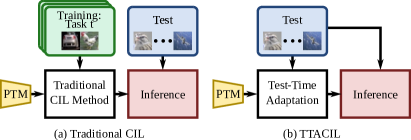
Figure 1: Comparison of traditional CIL methods with our TTACIL. (a) Traditional CIL methods entail training on each task’s training data, making it prone to forgetting. (b) In TTACIL we adapt the PTM directly on the test instances using Test-Time Adaptation. After inference, the model is reset back to the original checkpoint. It ensures a better stability-plasticity trade-off.

The status quo in the CIL literature entails training the network (typically ResNets [21]) from scratch on the data from the current session (or task), alongside optimizing a regularization objective for mitigating forgetting [44, 67]. Recently with the rise of the generalist and expressive vision transformer (ViT) based [13] pre-trained models (PTMs), trained on large datasets (e.g., ImageNet [11]), leveraging the PTMs for the incremental tasks has emerged as a viable alternative [70, 71, 69, 64, 80] in CIL. Using PTMs significantly enhances the data efficiency of CIL and consistently outperforms the traditional CIL methods trained from scratch [78]. For instance, Zhou et al. [80] demonstrated that adopting the nearest class mean (NCM) [45] classification approach using a frozen PTM leads to a competitive performance, surprisingly outperforming several state-of-the-art CIL approaches. This simple yet strong baseline reaffirms the generalizability of PTMs for CIL.

Although frozen PTMs attain impressive performance in CIL, such an approach suffers from intransigence, which is characterized by a lack of freedom to learn new tasks [8]. To remedy this issue an array of CIL methods have been proposed that rely on parameter efficient tuning, such as prompt-tuning [70, 71] or fine-tuning adapters [80], while keeping the PTM weights frozen. In particular, ADapt And Merge (ADAM) [80] fine-tunes the adapters only on the first task, among the sequences of all the tasks in a dataset, to adapt to the dataset at hand. While this approach partially addresses the stability-plasticity trade-off [47] by not fine-tuning the second task onwards, it still can not fully adapt to the whole dataset containing very heterogeneous tasks. On the contrary, sequentially fine-tuning the adapters on each task will result in poor stability on previous tasks.

In this work, we offer an alternative perspective to better address the stability-plasticity dilemma. Instead of fine-tuning the adapters to instill new knowledge on each task, we propose to bypass this repetitive training and adapt the PTM to the new task by performing test-time adaptation (TTA) [76] on each test instance (see Fig. 1). TTA, which was originally conceived for mitigating domain shift [54] between a pre-trained source model and the unlabelled data in the target domain [38], in the context of CIL it enables: (i) plasticity by fine-tuning only a small subset of parameters (e.g., Layer Norm [3]) of the PTM on the unlabelled test instance to adapt to any new task at hand, and (ii) stability by resetting the model to the original PTM checkpoint after each test instance. Unique to our proposed method, it preserves the generalizable representation power of the PTM, while being malleable enough to learn new tasks. We therefore call our method as Test-Time Adaptation for Class-Incremental Learning (or TTACIL). Note that the goal of this work is neither to propose a novel method for TTA nor to propose a new setting for CIL, but to demonstrate that TTA is a promising solution for effective CIL.

More formally, our TTACIL is composed of two phases. In Phase I, similar to ADAM, we fine-tune randomly initialized adapters on the first task’s training data in order to learn task-specific and loosely dataset-specific features (see Sec. 3.3). Note that training on the first task does not aid in forgetting. In Phase II, we perform TTA directly on the unlabelled test instances of each task by unlocking exclusively the learnable parameters pertaining to the Layer Norm (see Sec. 3.4). This allows the network to adapt to the intricate task-specific features from subsequent tasks, while not deviating too far from the generalizable PTM representations. As a TTA objective, we minimize the entropy of the marginal distribution of the model predictions on augmented versions of a given test sample [76]. In practice, we find that only a single adaptation step (or gradient update) is sufficient to reach good performance without incurring higher computation costs at inference. To eliminate batch dependency we adopt episodic TTA [76], i.e., by resetting the model back to the base model in Phase I.

The novel perspective of addressing CIL with TTA presents us with several benefits: (i) it cuts computation during training time by limiting the training to just the first task, (ii) it does not lead to irreversible forgetting on the previous tasks as the model is reset after every adaptation on a new task, hence capitalizing the strong generalizability of PTMs, (iii) it is robust to unforeseen alterations to test samples, such as synthetic corruptions and perturbations [23], a critical aspect which has been overlooked in CIL, and (iv) it is highly parameter-efficient while being state-of-the-art in many CIL benchmarks. Unlike many CIL methods, our TTACIL is intuitive and simple to implement.

In summary, our contributions are the following: (i) We bring a paradigm shift in CIL with our proposed TTACIL by successfully demonstrating that TTA is a potent and efficient solution for CIL in the era of large PTMs. (ii) We are also the first to highlight the need to evaluate the robustness of CIL methods against common corruptions. Our TTACIL is implicitly robust to such corruptions. (iii) We extensively benchmark PTM-based CIL methods, including benchmarks that have large domain gaps with the pre-training data. Our TTACIL outperforms state-of-the-art CIL methods on both clean and corrupted data.

2 Related Work

Class-Incremental Learning is an active area of research (see the surveys in [44, 5, 67, 50]) that deals with incrementally expanding the knowledge of a model to recognize new classes by training on labelled data arriving in sessions. While learning the new classes the model tends to forget previously acquired information due to the phenomenon called catastrophic forgetting [18]. Therefore, the CIL methods aim at simultaneously balancing the knowledge acquisition (i.e., plasticity) and the knowledge retention (i.e., stability) capabilities of the model [47].

The CIL methods can be broadly categorized into four distinct groups: (i) Weight regularization CIL methods [33, 39, 73, 36, 2, 8] aim at preventing a drift in the weights of the network which are relevant to the previous tasks. (ii) Data regularization CIL methods [31, 37, 55, 27, 7, 41, 12, 15] instead aim at preventing a drift in the network activation by employing knowledge distillation [26]. (iii) Memory rehearsal CIL methods reduce forgetting by storing and replaying a small number of exemplars [55, 6, 7, 53], or by generating synthetic images [60, 49] or features [72]. (iv) Architecture growing CIL methods [57, 43, 42, 58] that dynamically increase the capacity of the network through allocating task-specific learnable parameters to prevent interference between tasks, and hence reduce forgetting. Our proposed TTACIL is unique from most of the existing CIL literature as it operates directly at test-time. Although similar in spirit with GDumb [53], which re-trains the network at test-time from scratch using exemplars from the memory, our TTACIL is rehearsal-free and requires only a single gradient update on the test sample to be ready for inference.

CIL with Large Pre-Trained Models. With the introduction of large PTMs [13] the field of CIL has seen a rapid progress [71, 70, 59, 80, 81, 75]. It is mainly driven by the fact that PTMs are highly generalizable to downstream tasks and tuning only a small subset of parameters is sufficient to obtain good performance. Broadly speaking, all the PTM-based CIL methods can be classified under two categories. The first category consists of prompt-tuning [30] based CIL methods [71, 70, 64, 59] that keep the PTM frozen and aim to train a set of learnable tokens (or prompts) on the training data to learn task-specific features. At inference, they query the prompt pool to retrieve a prompt pertaining to the test instance, and then condition the frozen PTM with the selected prompt. The prompt-tuning methods mostly differ in how the prompts are learned and how they are selected during inference. For instance, DualPrompt [70] decomposes the prompts into general and expert prompts, whereas CODA-Prompt [61] refines the prompt selection using an attention mechanism. The second category consists of CIL method ADAM [80] that fine-tune adapters [28] while keeping the PTM weights unaltered. To prevent catastrophic forgetting ADAM limits the fine-tuning to only the first task and keeps the model frozen for rest of the tasks. Differently from ADAM, in our TTACIL we encourage adaptivity via test-time adaptation on every new task and then reset it back to ensure stability. Moreover, unlike the prompt-tuning methods, the pipeline of our TTACIL is much simpler.

Test-Time Adaptation (TTA) has been proposed to improve the performance of a pre-trained model (trained on source data) on out-of-distribution test (or target) data, exhibiting domain-shift, by adjusting the model parameters using the unlabelled test samples [38, 66, 62, 40, 76, 9, 4]. In particular, the co-variate shift is simulated with synthetic corruptions [23] (e.g., Gaussian noise, blur, shot noise) or natural shifts (e.g., sim to real [51]). The common theme among all TTA methods is to optimize an unsupervised loss (e.g., entropy minimization [20]) using the test instance and update either all the parameters of the network [76] or only a subset (e.g., Batch Normalization layers [66]). Post adaptation, the resulting model is used for inference on the test instance, and after which it is either reset back to the original checkpoint [76] or directly used for the next adaptation steps [66]. Different from the original motivation of TTA – to reduce domain-shift between train and test data having overlapping classes – we exploit the generalizable PTM in CIL to adapt it on tasks (or datasets) containing non-overlapping set of classes. To the best of our knowledge, we are the first to demonstrate how TTA can also be seamlessly used for CIL and the effectiveness in CIL.

3 Proposed Framework

3.1 Problem Formulation and Overview

CIL involves learning from a data stream that introduces new classes and aims to construct a unified classifier [55]. The training process consists of a sequence of $T$ training tasks, denoted as $\mathcal{D}=\{\mathcal{D}^{1},\mathcal{D}^{2},\cdots,\mathcal{D}^{T}\}$ with incremental data $\mathcal{D}^{t}$ for each new task, each composed of $K^{t}$ classes; hence, we have $K=\sum_{t=1}^{T}K^{t}$ total number of classes. For each class $k$, the number of training samples is $N_{k}$.

In this context, ${\bf x}_{i}$ refers to a training instance belonging to the class $y_{i}\in Y^{t}$, where $Y^{t}$ is the label space of task $t$. In our case, there is no overlap in the label spaces between different tasks, i.e., $Y^{t}\!\cap\!Y^{t^{\prime}}\!=\!\varnothing$ for $t\!\neq\!t^{\prime}$. During the $t$-th training stage, only data from $\mathcal{D}^{t}$ can be accessed for model updates. Following the approach as in [71, 70], we assume the availability of a PTM, such as a ViT [13] trained on the ImageNet-21K dataset [56]. This pre-trained model serves as the initialization for the CIL model.

A successful CIL model $f$ acquires knowledge from new classes while preserving it from the previously encountered ones. The evaluation of the model’s capability is performed across all seen classes, denoted as $\mathcal{Y}^{T}\!=\!Y^{1}\!\cup\!\cdots\!\cup\!Y^{t-1}\!\cup\!Y^{t}$, after each incremental task $t$.

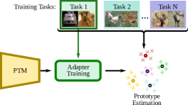
(a) Phase I: Training Procedure

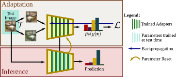
(b) Phase II: Test Time Adaptation with model reset.

Figure 2: Our TTACIL is composed of two phases. In Phase I, we fine-tune adapters on the first task’s training data in order to learn task-specific features. In Phase II, we perform TTA directly on the unlabelled test instances of each task. This allows the network to adapt to the intricate task-specific features from subsequent tasks, while not deviating too far from the generalizable PTM representations.

To address this problem, we introduce TTACIL, a novel method designed to harness the expressive power of PTMs while enabling plasticity and enhanced robustness. Our approach leverages prototype-classifiers (see Sec. 3.2) and enables plasticity via two complementary strategies: (i) an adaptation strategy is employed at training time to adapt the feature representations of the PTM as detailed in Sec. 3.3; (ii) a test-time adaptation further enhances adaptation, as explained in Sec. 3.4. An overview of TTACIL is displayed in Fig. 2 and summarized in Algorithm 1.

3.2 Prototype-classifier with PTMs

Inspired by [55, 46], we employ an approach called “Prototype-Classifier” to transfer PTM knowledge for incremental tasks. We denote $E_{\theta}$ as the features extractor of the PTM model $f$, having $\theta$ as its parameters. We employ $E_{\theta}$ to estimate the class prototypes $\bm{c}_{k}$, with $k\!=\!1,...,K$. To achieve this, we freeze the embedding function $E_{\theta}$ and compute the average embedding for each class in the current task ${\mathcal{D}}^{t}$ as

$$\bm{c}_{k}=\frac{1}{N_{k}}{\sum_{j=1}^{|\mathcal{{D}}^{t}|}\delta_{y_{j},k}E_{\theta}({\bf x}_{j})},$$ (1)

where $\delta_{a,b}$ is the Kronecker delta. The averaged embedding $\bm{c}_{k}$ aims at capturing the most common pattern observed in each class. For a test instance ${\bf x}_{i}$, we estimate the probability of each class $k$ via the dot products between the image feature representation $\bm{z}_{i}\!=\!E_{\theta}({\bf x}_{i})$ and each prototype through:

$$p_{\theta}\left(y_{i}=k|\bm{z}_{i}\right)=\frac{\exp(\bm{z}_{i}\cdot\bm{c}_{k})}{\sum_{j}\exp(\bm{z}_{i}\cdot\bm{c}_{j})}.$$ (2)

For us the model CIL $f$ includes the feature extractor $E_{\theta}$ and the prototype-classifiers. Our experiments show that prototype-classifiers can achieve competitive performance even without fine-tuning on the target dataset (refer to Sec. 4.2). However, when the downstream datasets exhibit a domain shift compared to the dataset used for model pre-training, the performance drops. Such drop is evident especially when the new data demands specific domain insights or shows significant concept drift [1, 25].

To address this issue, we proceed in two adaptation phases: Adapting PTM to new Tasks, followed by Test-Time Model Refinement. In the next sections, we will detail these two stages.

3.3 Phase I: Adapting PTMs to New Tasks

To allow a certain level of plasticity, we employ an adaptation process, which is based on the following observations: repeated adaptations to each new incremental task trigger catastrophic forgetting and weaken generalization [35]. Thus, our approach performs feature adaptation primarily during the first task. For the following tasks, the feature representation remains unchanged. This ensures that the model acquires domain-relevant insights early on without facing catastrophic forgetting.

In the first task, we adapt $E_{\theta}$ by inserting lightweight modules inside each layer called Adapters [29]. The adapter parameters, denoted as $\phi$, are learned on the data $\mathcal{D}^{1}$ while the parameters $\theta$ of $E_{\theta}$ remain frozen. The adaptation is done by minimizing a Cross-Entropy loss using stochastic gradient descent. Importantly, the parameters $\phi$ represent a tiny proportion of the total number of parameters in $E_{\theta,\phi}$ (about $1\%-3\%$) to prevent over-fitting on $\mathcal{D}^{1}$.

This procedure provides an adapted features extractor $E^{*}_{\theta,\phi}$ with domain-specific knowledge.

3.4 Phase II: Test-Time Model Refinement

After the initial adaptation on the first task, our model may still provide unsatisfactory results when it encounters visual content different from the past tasks. To tackle this, we propose to employ Test-Time Adaptation (TTA) which enables plasticity without suffering from catastrophic forgetting. This TTA phase consists of a slight feature adaptation on the test images in an unsupervised fashion. After evaluation on each test batch, our model is reset to the initial state $E_{\theta,\phi}^{*}$ to maintain generability, and we prevent catastrophic forgetting [17, 76]. An additional reason for adopting a TTA approach is that it enhances the robustness of our model against noisy and corrupted samples during inference [62, 66].

Inspired by MEMO [76], given a test sample ${\bf x}_{i}$, an adapted PTM model (from phase I), and a set of image Transformations $\mathcal{T}$, we pick $M$ random transformations $\{\tau_{1},\ldots,\tau_{M}\}$ from $\mathcal{T}$ and apply them to ${\bf x}_{i}$ in order to produce a batch of augmented data $\{\tilde{{\bf x}}_{i,1},\ldots,\tilde{{\bf x}}_{i,M}\}$. The marginal output distribution with respect to the augmented points is given by:

$$\bar{p}_{\theta,\phi}(y|{\bf x}_{i})\approx\frac{1}{M}\sum_{m=1}^{M}p_{\theta,\phi}(y|\tilde{{\bf x}}_{i,m}).$$ (3)

We propose to adapt the model by minimizing the entropy of its marginal output distribution over augmentations (3):

$$\mathcal{L}(\theta,\phi;{\bf x}_{i})=-\sum_{y\in\mathcal{Y}}\bar{p}_{\theta,\phi}(y|{\bf x}_{i})\log\bar{p}_{\theta,\phi}(y|{\bf x}_{i})\,.$$ (4)

In the process of minimizing (4), the model is driven to achieve both high confidence and invariance to input augmentations. Specifically, the entropy term $\bar{p}_{\theta,\phi}(\cdot|{\bf x}_{i})$ reaches its minimum value when the model delivers consistent and confident predictions, regardless of the particular data augmentation applied. The motivation for optimizing the model to yield more confident predictions is grounded in the belief that the decision boundaries distinguishing classes are situated in areas of the data space with lower density [20, 76].

As $\bar{p}_{\theta,\phi}(y|{\bf x}_{i})$ is differentiable with respect to $\theta$ based on the loss defined in (4), we can employ gradient-based optimization directly to adapt $\theta$. Test-time adaptation requires careful selection of parameters [48], our adaptation procedure focuses solely on adapting the layer-norm parameters [3], unlike MEMO [76] which finetunes all the model. We found that adapting all the parameters hurts the performance (see Sec. 4.3). Only one gradient step per test point is empirically determined to be sufficient for achieving improved performance, with less inference time overhead. Then, we utilize the adapted model $f_{\theta^{{}^{\prime}},\phi}$ to make predictions on the test input ${\bf x}_{i}$.

Algorithm 1 The pipeline of proposed TTACIL.

0:  Sequence of $T$ tasks, ${\mathcal{D}}\!={{\mathcal{D}}^{1},...,{\mathcal{D}}^{T}}$, and pre-trained model $f$

1:  Phase I: Adapting PTMs to New Tasks

2:     Adapt model $f$ using Adapters on ${\mathcal{D}}^{1}$.

3:  Phase II: Test-Time Model Refinement

4:  for a batch ${\mathcal{X}}$ in ${\mathcal{D}}_{test}^{t}$ do

5:     Reset the model to the initial state $f_{\theta,\phi}$.

6:     for iteration $n=1\cdots N$ do

7:        Sample transformations from $\mathcal{T}$ and apply to ${\mathcal{X}}$.

8:        Calculate predictions via (3).

9:        Adapt parameters via (4).

10:     end for

11:  end for

12:  return  predictions for all ${\bf x}_{i}\in{\mathcal{D}}_{test}^{t}$.

4 Experiments

Table 1: Average ($\bar{\mathcal{A}}$) and last performance ($\mathcal{A}_{T}$) comparison on seven datasets with ViT-B/16-IN21K backbone. ‘IN-R/A’ stands for ‘ImageNet-R/A,’ and ‘OmniBench’ stands for ‘OmniBenchmark’. LwF, L2P and DualPrompt results are from [80], except (5-datasets) noted ’*’ from [70]. $\dagger$ indicates results reported in the original paper. The best performance is in bold, and the second best is underlined.

Method	CIFAR100-Inc5		CUB-Inc10		IN-R-Inc5		IN-A-Inc10		OmniBench-Inc30		VTAB-Inc10		5-datasets-Inc10∗		Average
	$\bar{\mathcal{A}}$	${\mathcal{A}_{T}}$	$\bar{\mathcal{A}}$	${\mathcal{A}_{T}}$	$\bar{\mathcal{A}}$	${\mathcal{A}_{T}}$	$\bar{\mathcal{A}}$	${\mathcal{A}_{T}}$	$\bar{\mathcal{A}}$	${\mathcal{A}_{T}}$	$\bar{\mathcal{A}}$	${\mathcal{A}_{T}}$	$\bar{\mathcal{A}}$	${\mathcal{A}_{T}}$	$\bar{\mathcal{A}}$
Finetune	38.90	20.17	26.08	13.96	21.61	10.79	21.60	10.96	23.61	10.57	34.95	21.25	31.12	27.42	28.26
Finetune Adapter [10]	60.51	49.32	66.84	52.99	47.59	40.28	43.05	37.66	62.32	50.53	48.91	45.12	47.34	44.17	52.11
LwF [37]	46.29	41.07	48.97	32.03	39.93	26.47	35.39	23.83	47.14	33.95	40.48	27.54	-	-	-
L2P [71]	85.94	79.93	67.05	56.25	66.53	59.22	47.16	38.48	73.36	64.69	77.11	77.10	81.14	-	71.18
DualPrompt [70]	87.87	81.15	77.47	66.54	63.31	55.22	52.56	42.68	73.92	65.52	83.36	81.23	88.08	-	75.22
Prototype-Classifier	86.27	81.27	90.79	86.77	61.63	54.33	58.66	48.52	80.63	73.33	85.99	84.44	72.90	83.16	76.70
ADAM $\dagger$ [80]	90.65	85.15	92.21	86.73	72.35	64.33	60.53	49.57	80.75	74.37	85.95	84.35	-	-	-
ADAM [80]	90.87	85.15	91.06	86.73	72.35	64.33	60.21	49.57	79.70	55.24	85.95	84.35	72.97	83.14	79.79
SLCA [75]	94.54	91.19	84.70	81.76	74.10	69.73	61.98	56.48	80.40	72.05	88.92	82.65	82.67	80.11	81.04
TTACIL (w/o Phase I)	85.48	81.04	90.56	86.85	61.76	54.42	58.62	48.65	80.65	73.30	90.63	85.88	73.74	83.82	77.39
TTACIL	91.88	87.60	90.94	86.39	78.24	69.95	65.67	56.10	81.13	76.39	90.94	84.10	83.61	80.91	83.20

Table 2: Average performance ($\bar{\mathcal{A}}$) comparison with ViT-B/16-IN21K as the backbone on three corrupted benchmarks CIFAR100-C, VTAB-C and OmniBench-C with Level-5 noise corruptions [24]. The best performance is in bold, and the second best is underlined.

Method	CIFAR100-C				VTAB-C				OmniBench-C
	Gauss.	Shot	Impul.	Avg.	Gauss.	Shot	Impul.	Avg.	Gauss.	Shot	Impul.	Avg.
Prototype-Classifier	35.52	39.05	46.89	40.48	69.64	72.31	58.18	66.71	77.44	78.43	75.07	76.98
ADAM [80]	37.52	48.73	65.03	50.43	71.10	74.11	58.98	68.06	79.45	79.57	77.76	78.93
TTACIL	47.33	51.45	67.89	55.56	71.58	74.23	59.44	68.42	79.66	79.59	78.54	79.26

4.1 Experimental setup

Datasets and settings. We validate our method on as many as seven CIL benchmarks. In detail, following the work in [80] we experiment with CIFAR100 [34], CUB200 [65], ImageNet-R [22], ImageNet-A [25], OmniBench [77], 5-Datasets [71] and VTAB [80]. All these benchmarks offer diverse levels of difficulty in terms of high task heterogeneity (e.g., 5-Datasets, VTAB) or large domain gap with respect to ImageNet (e.g., ImageNet-A). For the experiments on robustness, we pick three benchmarks: CIFAR100-C [24], OmniBench-C, and VTAB-C, where “C” stands for corrupted counterparts of the original benchmarks. In this work, we introduce the VTAB-C and OmniBench-C by adding the same corruptions as in CIFAR100-C to the original testing sets of VTAB and OmniBench benchmarks, respectively.

We follow the incremental settings established in [80], i.e., by adopting an increment per task of three types: 5 classes (Inc5) for CIFAR100 and ImageNet-R; 10 classes (Inc10) for CUB200, ImageNet-A, VTAB and 5-Datasets; and 30 classes (Inc30) for OmniBench. The same increments and task orders are followed in the robustness experiments. Finally, we evaluate all the methods in task-agnostic manner, i.e., without having access to the task-id at inference. More details are available in the Supp. Mat.

Implementation details. Following ADAM [80] we have used ViT-B/16 [14], initially pre-trained on ImageNet-21K and further fine-tuned on ImageNet-1K, as a backbone. For Phase I, we trained the adapters (one adapter per ViT block) using Stochastic Gradient Descent (SGD) with momentum for 20 epochs, with an initial learning rate of 0.01 that undergoes cosine annealing. In Phase II we have used a batch size of 16 and augmented each test sample 8 times using random image transformations [76]. As mentioned before, for one mini-batch we do one gradient step in Phase II to obtain the adapted model. The learning rate and weight decay are set to 0.01 and 0, respectively. We ran all our experiments on a single Tesla A100 GPU.

Baselines and competitors. We have compared our proposed TTACIL with the competitor PTM-based CIL methods that are state-of-the-art: LwF [33], L2P [71], DualPrompt [70], ADAM[80] and SLCA [75]. All methods are initialized with the same PTM (ViT-B-16 [13]) pre-trained on Imagenet-21K. Additionally, we have compared with two more baselines: Finetune and Finetune Adapter [10]. Evaluation Metrics. In alignment with Rebuffi et al. [55], we denote the Top-1 accuracy achieved at the end of the $t$-th task as $\mathcal{A}_{t}$. We employ two key performance indicators: (i) $\mathcal{A}_{T}$, representing the Top-1 accuracy after learning the final task, and (ii) $\bar{\mathcal{A}}$, calculated as the average Top-1 accuracy while learning progresses in incremental steps, which is formally defined as $\bar{\mathcal{A}}=\frac{1}{T}\sum_{t=1}^{T}\mathcal{A}_{t}$.

4.2 Main results

Results on standard CIL benchmarks. We report in Tab. 1 the empirical evaluation on the standard CIL benchmarks, where we compare our proposed TTACIL with all the competitors. From the table, it is evident that TTACIL performs truly well, with an average accuracy $\bar{\mathcal{A}}$ of 83.15% which is the highest amongst all of the competitor methods. In some benchmarks such as CIFAR100, CUB200, and 5-Datasets our TTACIL is the second best. Notably, except in CUB200, our TTACIL consistently outperforms ADAM [80] on all the benchmarks. This highlights that adaptivity (or plasticity) is indeed important for learning task-specific features on each task. If training is limited till the first task, as done in ADAM, it leads to a drop of 3.41% in average performance (79.79% vs 83.20%). Contrarily, if the adapters are fine-tuned on each task, as denoted by the Finetune Adapter baseline in Tab. 1, the final performance drops drastically to 52.11%. This is due to the severe forgetting of the previous tasks. Contrarily, our TTACIL allows room for plasticity while not running into severe forgetting after adapting to each test sample due to model reset.

Although our TTACIL w/o Phase I, as reported in Tab. 1, lags behind some state-of-the-art methods by some points, it still improves over Prototype-Classifier by +0.69%. This again highlights that the frozen PTMs are sub-optimal when it comes to datasets with data distribution different from the pre-training datasets. For instance, in the VTAB benchmark our TTACIL w/o Phase I achieves an improvement of +4.64% over Prototype-Classifier that uses only frozen PTM features. Despite the simplicity, our TTACIL (and TTACIL w/o Phase I) outperforms all very complex prompt-tuning methods such as L2P and DualPrompt by several points on average. Thus, for real-life applications our TTACIL can serve as a preferred solution to CIL.

Results on CIL benchmarks with corruptions. In Tab. A2 we report the empirical evaluation on CIL benchmarks with different kinds of noise corruptions (of level 5 [23]), where we compare our proposed TTACIL with the competitors. In ADAM and our TTACIL, we exclude training on the clean samples from every task, except the first task.

The Prototype-Classifier exhibits the worst performance as it solely relies on the representation learned from the pre-training dataset. In ADAM, which trains the network on the training data from the first task, shows an improvement in the performance due to better adaptivity with respect to the Prototype-Classifier. With our proposed TTACIL we achieve the best performance as it further allows the model to adapt towards every subsequent task. In particular, the gain in performance is significant for CIFAR100-C where our proposed TTACIL outperforms ADAM by +5.13%.

In summary, our proposed TTACIL satisfies two desiderata: (i) improved adaptivity to new tasks, and (ii) robustness to corruptions by refining its predictions on the corrupted test instances during test-time. We report the results on other types of corruptions in the Supp. Mat.

4.3 Ablation analysis

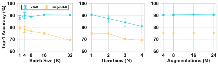
Figure 3: Ablation of TTACIL on VTAB and Imagenet-R benchmarks, based on varying batch size (left), adaptation iterations (center), and batch size (right).

Effect of task ordering. In Fig. 4 we demonstrate the influence of task order on the CIL performance, especially in the case of heterogeneous tasks. We choose to perform experiments on the 5-Datasets benchmark as it contains five very heterogeneous datasets: SVHN, MNIST, CIFAR10, NotMNIST, and FashionMNIST. Here we mainly compare our TTACIL with ADAM as both the methods undergo training on the first task’s data.

From Fig. 4, we notice that different task orders yield various performances for TTACIL and ADAM, indicating that the first task plays an important role in determining the final performance. However, in all the task orderings our TTACIL outperforms ADAM by big margins, with the highest margin (+10.29%) obtained in the tasks of order SVHN $\rightarrow$ MNIST $\rightarrow$ CIFAR10 $\rightarrow$ NotMNIST $\rightarrow$ FashionMNIST. This highlights that the data from the second task onwards, despite unlabelled, offer a learning signal, which is efficiently exploited by our TTACIL during Phase II. Differently, as ADAM does not offer any plasticity after the first task it fails to improve the adaptivity on future tasks.

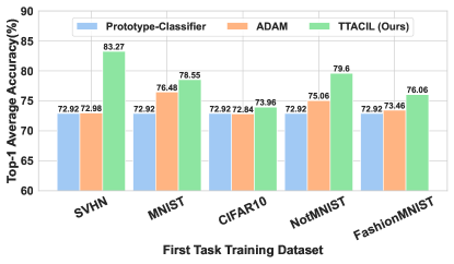
Figure 4: Comparative performance analysis of Prototype-Classifier, ADAM and our TTACIL when subjected to different task orderings. The first training task is indicated on the x-axis. The y-axis corresponds to the average performance across all the five-dataset benchmark.

We can also observe that when the first task is CIFAR10, a dataset very different from the other tasks, our TTACIL can still yield performance gain over ADAM and Prototype-Classifier. These results are promising since they indicate that TTACIL is a relevant solution even when the domain shifts in future tasks are potentially large [52].

Effect of the adaptation parameters. The experiments presented in Tab. 3 focus on evaluating different parameters to adapt during Test-Time Model Refinement phase. We compare the performance of four adaptation approaches: (i) no TTA – we do not apply test-time adaptation (equivalent to ADAM [80]); (ii) All – we adapt all the parameters of the model; (iii) Adapter – we adapt only the parameters of the adapter; and (iv) Norm – we adapt only the Layer Norm parameters.

Table 3: Evaluation of different parameters subject to optimization during test-time used in TTACIL. Average performance ($\bar{\mathcal{A}}$) is reported for VTAB and Imagenet-R (higher is better $\uparrow$). Number of trainable parameters in Million (M) (lower is better $\downarrow$).

	# of Par. (M) $\downarrow$	VTAB $\uparrow$	Imagenet-R $\uparrow$
No TTA	0	85.68 $\pm$ 2.44	73.58 $\pm$ 1.11
All	87	43.26 $\pm$ 1.15	26.02 $\pm$ 0.39
Adapter	1.2	89.89 $\pm$ 0.64	75.28 $\pm$ 0.97
Norm	0.04	90.52 $\pm$ 0.64	75.21 $\pm$ 1.02

When all the parameters are subjected to test-time adaptation, i.e., in All, the model has 87 million trainable parameters. In that case, it leads to a VTAB accuracy of 38.85% and an Imagenet-R accuracy of 22.31%. This performance is notably lower than the other configurations, likely due to the inherent complexity of adapting to such a vast parameter space with few samples, and one optimization iteration. In contrast, with Adapter baseline, where only the parameters in the adapter layers are updated, the number of trainable parameters is significantly reduced to 1.2 million, leading to a clear gain in performance on both datasets (VTAB at 89.41% and Imagenet-R at 74.76%). However, the best performance-parameter comes from the Norm variant that updates only the Layer Norm parameters, achieving the best and second-best performance while using only 0.04 million parameters.

Effect of the batch size. We ablate the effect of varying the batch size on the final performance in Fig. 3 (left). Our findings, averaged over these 3 seeds, reveal a complex relationship between batch size and model performance. Specifically, performance on the “VTAB” dataset reaches about 90% when the batch size approaches $4$ and remains almost constant for larger batch sizes. On the contrary, we observe an important decrease in performance on the Imagenet-R dataset when increasing the batch size. This behavior could be potentially explained by a mix of both low and high-entropy samples that could adversely affect TTA [48].

Effect of the number of adaptation iterations. In this study our goal is to quantify the influence of iterative adjustments during Phase II, the test-time refinement stage of the TTACIL. The results are summarized in Fig. 3 (middle). The results show that the performance decreases when increasing the number of test-time iterations on both datasets. Specifically, performance on VTAB descends from an initial 90.55% with one iteration to 80.78% at four iterations. A congruent decrement is observed in Imagenet-R, where the accuracy declines from 75.05% to 69.13% as the iteration count is augmented.

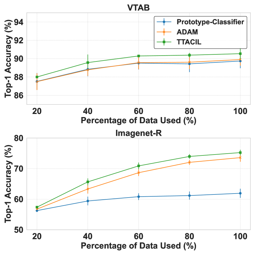
Figure 5: Ablation study on data efficiency. The plots showcase the top-1 accuracy on the VTAB and Imagenet-R datasets with varying percentages of training data used. TTACIL consistently outperforms other methods, especially in lower data regimes, highlighting its robustness to data scarcity.

This performance drop may be due to the model’s propensity for overfitting to low-entropy samples as discussed in [48]. Although this overconfidence enhances the model’s accuracy in these specific instances, it undermines its broader generalization capabilities. This leads to inaccuracies in classifying more complex or higher-entropy samples within the same batch, highlighting a nuanced trade-off between adaptability and overfitting during the test-time adjustment phase.

Effect of the number of Augmentations per adaptation iteration. We analyze the effect of varying the set of augmentations used in the TTA phase. We report the final performance in Fig. 3 (right) using a varying number of augmentations, where the results are aggregated across the 3 seeds. They show that TTACIL consistently maintains a high accuracy across both the VTAB and Imagenet-R datasets. It is important to mention that while increasing the number of augmentations may seem advantageous, it introduces additional computational overhead during inference, warranting careful consideration. Thus, it is recommended to keep a small number of augmentations in the range of $M\in[1,\cdots,8]$ since the performance of TTACIL does not benefit significantly from large $M$.

Data Efficiency. As described in Sec. 3, training data is only used for prototype estimation (except for task 1) making our model potentially less prone to overfitting. However, the lack of plasticity could also induce difficulty in benefiting from large training sets. For deeper insights, we propose to analyze the performance of TTACIL considering training datasets of varying sizes. The results are visualized in Fig. 5.

First, we observe that with only 20% of the training data, TTACIL achieves a Top-1 accuracy of 88% on the VTAB dataset, compared to 87.01% by Prototype-Classifier and 86.89% by ADAM. The differences among baselines are smaller in the case of the Imagenet-R dataset. As the percentage of available training data increases, TTACIL’s advantage becomes even more prominent. At 60% of the training data, TTACIL registers an impressive 72% on Imagenet-R, whereas Prototype-Classifier and ADAM lag behind at 61.22% and 69.78%, respectively. Note that both ADAM and TTACIL use the same prototypes and undergo the same first task training. So, the difference in performance is caused by our TTA phase. Overall, these experiments show that, despite the limited plasticity of prototype-classifiers, TTACIL is capable of benefiting from larger training dataset.

Limitations. The main limitations of TTACIL are its computational complexity and its high inference time. The TTA phase requires extra computation before each prediction but this increased computation cost should be viewed as a trade-off for improved plasticity and robustness. Practically, TTACIL can still perform inference at 8 frames per second when using a single TTA iteration. Furthermore, this increase in inference time is counterbalanced by TTACIL’s computational efficiency during training, i.e., by updating only the Layer Norm parameters in the first task.

5 Conclusions and Future works

We proposed TTACIL, a novel approach for addressing the long-standing task of CIL. In TTACIL we bypass repetitive training on each task and directly adapt to the unlabelled test samples during test time. We demonstrated that TTA, albeit simpler than many existing state-of-the-art CIL methods, is a promising solution for effective CIL. It preserves the generalizable representation power of the PTM while being malleable enough to learn on new tasks. Additionally, our TTACIL is more robust under common corruptions. As we future work, we would like to enhance the efficiency and performance of TTACIL. Specifically, we aim to explore advanced TTA techniques involving sampling methods [48, 68], to further accelerate inference time and to boost the method’s overall effectiveness.

Acknowledgements. This paper has been supported by the French National Research Agency (ANR) in the framework of its JCJC. Furthermore, this research was partially funded by Hi!PARIS Center on Data Analytics and Artificial Intelligence.

Supplementary Material

In this supplementary material, we provide more details about the experimental results mentioned in the main paper, as well as additional empirical evaluations and discussions. The supplementary material is organized as follows: In Section A, we evaluate the effect of task order. In Section B, provide additional evaluations on CIFAR100-C dataset. In Section C, reports the full experimental results ablation studies in the main paper. In Section E, we analyze the inference cost of TTACIL. In Section F, provides an ablation study about the Adapter size in TTACIL. In Section G, we detail the baselines, and datasets used in our experiments.

Appendix A Effect of Varying Task Sequence Orders

This section evaluates the adaptability of our proposed method TTACIL and compares it with ADAM in CIL scenarios on the 5-Datasets benchmark. We specifically delve deeper into the experiments discussed in Sec. 4.3 of the main paper, where we analyze the influence of task order. on the impact of the task order. We provide more detailed experimental results considering multiple task orders. The task sequences include variations with SVHN, MNIST, CIFAR10, NotMNIST, and FashionMNIST. Results are reported in Tab. A1. The orange cells corresponding to the first task, both ADAM and TTACIL have been trained on.

The results indicate the substantial influence of task sequence on model performance, highlighting the pivotal role of the initial task. TTACIL consistently surpasses ADAM in all sequences, with a maximum performance gain of +10.29% observed in the SVHN $\rightarrow$ MNIST $\rightarrow$ CIFAR10 $\rightarrow$ NotMNIST $\rightarrow$ FashionMNIST sequence. This suggests that TTACIL effectively leverages unlabeled data from subsequent tasks to improve its adaptability.

Table A1: Performance Comparison of ADAM [80] and TTACIL Across Varying Task Sequence Orders in Class-Incremental Learning. Top-1 accuracy is reported ($\uparrow$). Orange cells indicate the task that the model has been trained on. Model used in ViT-B/16 pre-trained on Imagenet-21K.

Method		SVHN	MNIST	CIFAR10	NotMNIST	FashionMNIST	Average
Prototype-Classifier		33.18	83.78	95.63	68.85	83.18	72.92
ADAM [80]	SVHN	33.44	83.84	95.62	68.85	83.14	72.98
	MNIST	92.44	93.95	72.77	83.00	40.22	76.48
	CIFAR10	97.24	67.97	83.63	31.33	84.04	72.84
	NotMNIST	71.02	83.66	38.20	86.51	95.89	75.06
	FashionMNIST	84.19	31.52	85.69	95.96	69.93	73.46
Ours	SVHN	95.13	96.48	67.33	78.43	78.96	83.27
	MNIST	97.89	76.15	82.35	83.09	53.28	78.55
	CIFAR10	98.95	70.37	83.24	35.03	82.19	73.96
	NotMNIST	88.67	83.82	59.16	92.76	73.61	79.60
	FashionMNIST	91.02	44.35	84.63	82.50	77.78	76.06

Appendix B Evaluation on CIFAR100-C with Level-5 Corruptions

We compare our method, TTACIL , with state-of-the-art methods on CIFAR100-C with Level-5 corruptions [24], as summarized in Tab. A2. The Prototype-Classifier performs poorly, yielding a 53.89% average accuracy, due to its reliance on pre-trained representations. ADAM improves upon this with a 66.57% average accuracy, courtesy of its initial task training.

In contrast, TTACIL achieves the highest average accuracy of 68.00%, outperforming ADAM by a significant margin of +5.13% on CIFAR100-C. These results substantiate TTACIL ’s superior adaptability and robustness to a variety of corruptions.

Table A2: Average and last performance comparison on seven datasets with ViT-B/16-IN21K as the backbone on CIFAR100-C with Level-5 corruptions [24]. The best performance is shown in bold, and the second-best is underlined.

Method	Noise			Blur				Weather				Average
	Gauss.	Shot	Impul.	Defoc.	Glass	Motion	Zoom	Snow	Frost	Fog	Brit.
Prototype-Classifier	35.52	39.05	46.89	59.78	31.29	56.99	65.04	64.41	63.99	50.13	79.68	53.89
ADAM [80]	37.52	48.73	65.03	78.02	39.80	74.59	79.27	76.92	73.34	70.50	88.59	66.57
TTACIL	47.33	51.45	67.89	78.52	42.70	75.00	79.00	75.31	72.49	69.20	89.09	68.00

Appendix C Ablation Study: Augmentations, Iterations, and Batch Size

This section provides the exact numerical values corresponding to Fig. 3 in the main paper. Please refer to the main paper for the corresponding analyses.

Table A3: Summarized results for VTAB and Imagenet-R datasets based on the number of augmentations $M$. (Mean $\pm$ Std. Dev.)

Augmentations (M)	VTAB$\uparrow$	Imagenet-R$\uparrow$
4	90.14 $\pm$ 0.72	75.30 $\pm$ 0.87
8	90.55 $\pm$ 0.61	75.22 $\pm$ 0.91
16	90.67 $\pm$ 0.39	75.26 $\pm$ 0.85
24	90.52 $\pm$ 0.36	75.23 $\pm$ 0.80

Table A4: Summarized results for VTAB and Imagenet-R datasets based on the number of iterations $N$. (Mean $\pm$ Std. Dev.)

Iterations (N)	VTAB$\uparrow$	Imagenet-R$\uparrow$
i=1	90.55 $\pm$ 0.52	75.05 $\pm$ 0.80
i=2	87.34 $\pm$ 3.05	74.77 $\pm$ 1.22
i=3	84.07 $\pm$ 3.53	70.14 $\pm$ 3.35
i=4	80.78 $\pm$ 5.45	69.13 $\pm$ 2.08

Table A5: Summarized results for VTAB and Imagenet-R datasets on the effect of batch size $B$ in TTACIL. (Mean $\pm$ Std. Dev.)

Batch Size (B)	VTAB$\uparrow$	Imagenet-R$\uparrow$
1	88.14 $\pm$ 1.71	79.11 $\pm$ 1.46
4	89.81 $\pm$ 2.62	78.22 $\pm$ 2.54
8	88.91 $\pm$ 2.87	76.62 $\pm$ 1.93
16	90.55 $\pm$ 0.58	75.05 $\pm$ 0.96
32	90.31 $\pm$ 0.09	69.12 $\pm$ 0.60

Appendix D Data Efficiency

This section presents the results of the ablation study conducted in Sec.4.3 of the main paper, which focuses on the data efficiency of our method TTACIL. Tab. A6 details the results presented in Fig. 4 in the main paper.

The study aims to examine how well TTACIL performs under varying degrees of data scarcity for training. We compare TTACIL’s performance against state-of-the-art methods like Prototype-classifier and ADAM across different datasets including VTAB and Imagenet-R.

Table A6: Performance comparison under varying data scarcity for training.

Training Data (%)	Prototype-classifier		ADAM		TTACIL (Ours)
	VTAB	Imagenet-R	VTAB	Imagenet-R	VTAB	Imagenet-R
20%	$87.52\pm 0.91$	$56.27\pm 0.45$	$87.49\pm 0.91$	$56.75\pm 0.40$	$88.00\pm 0.03$	$57.39\pm 0.29$
40%	$88.84\pm 0.76$	$59.41\pm 1.42$	$88.78\pm 0.66$	$63.34\pm 1.51$	$89.57\pm 0.88$	$65.66\pm 1.15$
60%	$89.51\pm 0.69$	$60.82\pm 1.10$	$89.56\pm 0.71$	$68.67\pm 1.08$	$90.29\pm 0.14$	$70.89\pm 1.09$
80%	$89.43\pm 0.90$	$61.18\pm 1.32$	$89.61\pm 0.75$	$72.05\pm 0.82$	$90.38\pm 0.24$	$73.98\pm 0.75$
100%	$89.74\pm 0.78$	$61.93\pm 1.49$	$89.90\pm 0.67$	$73.59\pm 1.34$	90.54 $\pm$ 0.64	75.24 $\pm$ 0.91

Appendix E Inference cost

In TTACIL, we introduce extra computation with an added optimization step before prediction, we now delve into a detailed analysis of the inference cost associated with TTACIL. By quantifying the inference time, we compare our method with two baselines: ADAM and Prototype-Classifier. Concretely, in TTACIL the inference time accounts for both TTA optimization and final prediction. We report the inference time (in milliseconds) averaged over five runs on an A100 (48GB) GPU. Our evaluation for TTACIL, we use one iteration $N\!=\!1$, with $M\!=\!8$ of augmentations.

Table A7: Inference Time Comparison in Milliseconds (ms). The results are an average of 5 runs. GFLOPS/GMACs are evaluated on batch-size $B\!=\!16$.

Batch Size	TTACIL	Prototype-Classifier	ADAM
B=16	1820	22	27
GFLOPS	85.45	33.72	34.18
GMACs	42.73	16.86	17.09

The computational overhead introduced by TTACIL is a trade-off for enhanced model plasticity and robustness. This increased computational cost during inference is offset by the method’s efficiency during training, where only the Layer Normalization parameters are updated in the initial task.

Tab. A8 quantifies the inference time of TTACIL across varying batch sizes $B$ and adaptation iterations $N$. The results emphasize the computational trade-offs involved in choosing different hyperparameters for TTACIL. It’s noteworthy that the rate of increase in execution time is not as steep when transitioning to larger batch sizes compared to smaller ones.

For instance, when comparing $B=1$ to $B=4$ at $N=1$, the execution time goes from 190 ms to 470 ms, an increase of 280 ms. However, the increase is less pronounced when the batch size goes from $B=8$ to $B=16$; the time for $N=1$ only increases by 770 ms, from 1000 ms to 1770 ms. This suggests that TTACIL demonstrates a form of computational efficiency with larger batch sizes in terms of execution time per unit increase in batch size.

Table A8: Execution Time comparison in Milliseconds (ms) concerning the number of adaptation iterations $N$/batch-size $B$.

		Iterations
		N=1	N=2	N=3	N=4
Batch-size	B=1	190	250	320	340
	B=4	470	630	680	810
	B=8	1000	1110	1270	1410
	B=16	1770	2140	2480	2460

Appendix F Adapter

The Adapter module, a bottleneck structure extensively studied in prior works [10, 29], enables fine-tuning of Vision Transformer (ViT) outputs. Composed of a down-projection $W_{\text{down}}\in\mathbb{R}^{d\times r}$, a non-linear activation function, and an up-projection $W_{\text{up}}\in\mathbb{R}^{r\times d}$, it facilitates dimensionality reduction and subsequent restoration. We adopt the AdaptMLP structure as introduced in AdaptFormer [10], effectively replacing ViT’s native MLP. Given the input $\mathbf{x}_{\ell}$ to the MLP, the output can be expressed as:

$$\text{MLP}(\mathbf{x}_{\ell})+s\cdot\text{ReLU}(\mathbf{x}_{\ell}W_{\text{down}})W_{\text{up}},$$ (A1)

where $s$ is an optional, learnable scaling parameter. As done in ADAM [80], during the adaptation phase, only adapter parameters are optimized, while the pre-trained weights of ViT remain fixed. We employ a hidden dimension $r$ of 16, resulting in approximately 0.3 million tunable parameters, a figure substantially lower than the 86 million parameters in the standard ViT-B/16 model.

Ablation Study on Adapter Sizes in TTACIL. Tab. A9 presents an ablation study examining the effect of varying adapter sizes $r$ on the average performance across multiple datasets such as VTAB, CIFAR100, and ImageNet-R. The reported trainable parameters also scale with the adapter size, giving us an insight into the computational cost involved.

The table reveals that increasing the adapter size does not substantially improve the model’s performance. For instance, while moving from $r\!=\!16$ to $r\!=\!256$, the average accuracy on the VTAB dataset slightly decreases from 89.65% to 88.65%. A similar trend is observed in the CIFAR100 and ImageNet-R datasets, with only marginal performance improvements or even slight deteriorations.

More importantly, the increase in adapter size comes at a substantial computational cost. The number of trainable parameters rises exponentially with the adapter size, going from 0.30 Million for $r\!=\!16$ to 4.73M for $r\!=\!256$. This not only increases the model’s complexity but also makes it computationally expensive to train.

In summary, our analysis underscores the conclusion that while increasing the adapter size in TTACIL may seem like a plausible avenue for performance improvement, it does not offer significant gains. Instead, it introduces computational inefficiencies due to the escalated number of trainable parameters, thereby questioning the trade-off between performance and computational cost.

Table A9: Comparison of TTACIL Average performance Across Different Adapter Sizes $r$ across datasets. Reported number of trainable parameters is in Million (M).

	$r=16$	$r=32$	$r=128$	$r=256$
Params (M)	0.30	0.60	2.37	4.73
VTAB	89.65	89.18	88.83	88.65
CIFAR100	90.25	90.14	89.25	89.04
ImageNet-R	74.72	75.03	75.39	74.99

Appendix G Baselines

We briefly outline the methods against which our approach is evaluated:

• Finetune: Incrementally trains on new datasets, inducing catastrophic forgetting as a consequence.

• Finetune Adapter [10]: Retains pre-trained weights while optimizing an adapter module. Classifiers specific to the current dataset $\mathbf{D}_{t}$ are fine-tuned, while those for previous classes are held constant.

• LwF [37]: Employs knowledge distillation [26] as a regularizer to mitigate forgetting, relying on the legacy model for soft target generation.

• L2P [71]: A leading PTM-based CIL method that maintains a frozen pre-trained model while optimizing a prompt pool. It incorporates a ’key-value’ pairing mechanism for prompt selection and leverages an auxiliary pre-trained model for prompt retrieval.

• DualPrompt [70]: An extension of L2P that utilizes two categories of prompts—general and expert—for enhanced performance. It also uses an additional pre-trained model for prompt retrieval.

• ADAM [80]: fine-tunes the adapters [10] only on the first task, among the sequences of all the tasks in a dataset, to adapt to the dataset at hand.

• SLCA [75]: improves the classification layer by modeling the class-wise distributions and aligning the classification layers in a post-hoc fashion.

Appendix H Datasets

We describe the datasets utilized in our study, summarized in Tab. A10. While CIFAR100, CUB200, and ImageNet-R are established CIL benchmarks [55, 70, 79], ImageNet is ill-suited for PTM-based CIL evaluation due to data overlap [71]. Consequently, we introduce four additional benchmarks characterized by non-overlap with ImageNet, substantial domain diversity, and large-scale, cross-domain instances.

• CIFAR100 [34]: Comprises 100 classes, 60,000 images—50,000 for training and 10,000 for testing.

• CUB200 [65]: Focuses on fine-grained visual categorization, containing 11,788 bird images across 200 subcategories, with 9,430 for training and 2,358 for testing.

• ImageNet-R [22]: Extended for CIL by [70], includes various styles and hard instances, totaling 24,000 training and 6,000 testing instances.

• ImageNet-A [25]: Features real-world adversarially filtered images, with 5,981 training and 1,519 testing instances.

• OmniBenchmark [77]: A diverse benchmark challenging PTM generalization, containing 89,697 training and 5,985 testing instances across multiple semantic realms.

• VTAB [74]: Encompasses 19 tasks across three categories—Natural, Specialized, and Structured. We select five datasets to construct a cross-domain CIL setting. Similar to ADAM [80], we select 5 to construct a cross-domain class-incremental learning setting, i.e., Resisc45, DTD, Pets, EuroSAT, and Flowers.

• 5-datasets [16]: a sequence of classification datasets including SVHN, CIFAR10, not-MNIST, Fashion-MNIST and, and MNIST.

Table A10: Introduction about benchmark datasets. ObjectNet, OmniBenchmark, and VTAB contain massive classes, and we sample a subset from them to construct the incremental learning task.

Dataset	# training	# testing	# Classes	Link
	instances	instances
CIFAR100	50,000	10,000	100	Link
CUB200	9,430	2,358	200	Link
ImageNet-R	24,000	6,000	200	Link
ImageNet-A	5,981	1,519	200	Link
ObjectNet	26,509	6,628	200	Link
OmniBenchmark	89,697	5,985	300	Link
VTAB	1,796	8,619	50	Link
5-datasets	180,869	506.906	50	Link

References

- [1] Amit Alfassy, Assaf Arbelle, Oshri Halimi, Sivan Harary, Roei Herzig, Eli Schwartz, Rameswar Panda, Michele Dolfi, Christoph Auer, Kate Saenko, et al. Feta: Towards specializing foundation models for expert task applications. arXiv preprint arXiv:2209.03648, 2022.
- [2] Rahaf Aljundi, Francesca Babiloni, Mohamed Elhoseiny, Marcus Rohrbach, and Tinne Tuytelaars. Memory aware synapses: Learning what (not) to forget. In ECCV, pages 139–154, 2018.
- [3] Jimmy Lei Ba, Jamie Ryan Kiros, and Geoffrey E. Hinton. Layer normalization, 2016.
- [4] Alexander Bartler, Andre Bühler, Felix Wiewel, Mario Döbler, and Bin Yang. Mt3: Meta test-time training for self-supervised test-time adaption. In International Conference on Artificial Intelligence and Statistics, pages 3080–3090. PMLR, 2022.
- [5] Eden Belouadah, Adrian Popescu, and Ioannis Kanellos. A comprehensive study of class incremental learning algorithms for visual tasks. Neural Networks, 135:38–54, 2021.
- [6] Pietro Buzzega, Matteo Boschini, Angelo Porrello, Davide Abati, and Simone Calderara. Dark experience for general continual learning: a strong, simple baseline. Advances in neural information processing systems, 33:15920–15930, 2020.
- [7] Francisco M Castro, Manuel J Marín-Jiménez, Nicolás Guil, Cordelia Schmid, and Karteek Alahari. End-to-end incremental learning. In ECCV, pages 233–248, 2018.
- [8] Arslan Chaudhry, Puneet K Dokania, Thalaiyasingam Ajanthan, and Philip HS Torr. Riemannian walk for incremental learning: Understanding forgetting and intransigence. In ECCV, pages 532–547, 2018.
- [9] Dian Chen, Dequan Wang, Trevor Darrell, and Sayna Ebrahimi. Contrastive test-time adaptation. In Proceedings of the IEEE/CVF Conference on Computer Vision and Pattern Recognition, pages 295–305, 2022.
- [10] Shoufa Chen, GE Chongjian, Zhan Tong, Jiangliu Wang, Yibing Song, Jue Wang, and Ping Luo. Adaptformer: Adapting vision transformers for scalable visual recognition. In NeurIPS, 2022.
- [11] Jia Deng, Wei Dong, Richard Socher, Li-Jia Li, Kai Li, and Li Fei-Fei. Imagenet: A large-scale hierarchical image database. In CVPR, pages 248–255, 2009.
- [12] Prithviraj Dhar, Rajat Vikram Singh, Kuan-Chuan Peng, Ziyan Wu, and Rama Chellappa. Learning without memorizing. In CVPR, pages 5138–5146, 2019.
- [13] Alexey Dosovitskiy, Lucas Beyer, Alexander Kolesnikov, Dirk Weissenborn, Xiaohua Zhai, Thomas Unterthiner, Mostafa Dehghani, Matthias Minderer, Georg Heigold, Sylvain Gelly, et al. An image is worth 16x16 words: Transformers for image recognition at scale. In ICLR, 2020.
- [14] Alexey Dosovitskiy, Lucas Beyer, Alexander Kolesnikov, Dirk Weissenborn, Xiaohua Zhai, Thomas Unterthiner, Mostafa Dehghani, Matthias Minderer, Georg Heigold, Sylvain Gelly, Jakob Uszkoreit, and Neil Houlsby. An image is worth 16x16 words: Transformers for image recognition at scale, 2021.
- [15] Arthur Douillard, Matthieu Cord, Charles Ollion, Thomas Robert, and Eduardo Valle. Podnet: Pooled outputs distillation for small-tasks incremental learning. In ECCV, pages 86–102, 2020.
- [16] Sayna Ebrahimi, Franziska Meier, Roberto Calandra, Trevor Darrell, and Marcus Rohrbach. Adversarial continual learning. In ECCV, pages 386–402, 2020.
- [17] François Fleuret et al. Test time adaptation through perturbation robustness. 2021.
- [18] Robert M French. Catastrophic forgetting in connectionist networks. Trends in cognitive sciences, 3(4):128–135, 1999.
- [19] Heitor Murilo Gomes, Jean Paul Barddal, Fabrício Enembreck, and Albert Bifet. A survey on ensemble learning for data stream classification. CSUR, 50(2):1–36, 2017.
- [20] Yves Grandvalet and Yoshua Bengio. Semi-supervised learning by entropy minimization. Advances in neural information processing systems, 17, 2004.
- [21] Kaiming He, Xiangyu Zhang, Shaoqing Ren, and Jian Sun. Deep residual learning for image recognition. In CVPR, pages 770–778, 2015.
- [22] Dan Hendrycks, Steven Basart, Norman Mu, Saurav Kadavath, Frank Wang, Evan Dorundo, Rahul Desai, Tyler Zhu, Samyak Parajuli, Mike Guo, et al. The many faces of robustness: A critical analysis of out-of-distribution generalization. In ICCV, pages 8340–8349, 2021.
- [23] Dan Hendrycks and Thomas Dietterich. Benchmarking neural network robustness to common corruptions and perturbations. 2019.
- [24] Dan Hendrycks and Thomas Dietterich. Benchmarking neural network robustness to common corruptions and perturbations. Proceedings of the International Conference on Learning Representations, 2019.
- [25] Dan Hendrycks, Kevin Zhao, Steven Basart, Jacob Steinhardt, and Dawn Song. Natural adversarial examples. In CVPR, pages 15262–15271, 2021.
- [26] Geoffrey Hinton, Oriol Vinyals, and Jeff Dean. Distilling the knowledge in a neural network. arXiv preprint arXiv:1503.02531, 2015.
- [27] Saihui Hou, Xinyu Pan, Chen Change Loy, Zilei Wang, and Dahua Lin. Learning a unified classifier incrementally via rebalancing. In CVPR, pages 831–839, 2019.
- [28] Neil Houlsby, Andrei Giurgiu, Stanislaw Jastrzebski, Bruna Morrone, Quentin De Laroussilhe, Andrea Gesmundo, Mona Attariyan, and Sylvain Gelly. Parameter-efficient transfer learning for nlp. In ICML, pages 2790–2799, 2019.
- [29] Neil Houlsby, Andrei Giurgiu, Stanislaw Jastrzebski, Bruna Morrone, Quentin de Laroussilhe, Andrea Gesmundo, Mona Attariyan, and Sylvain Gelly. Parameter-efficient transfer learning for nlp, 2019.
- [30] Menglin Jia, Luming Tang, Bor-Chun Chen, Claire Cardie, Serge J. Belongie, Bharath Hariharan, and Ser-Nam Lim. Visual prompt tuning. In ECCV, pages 709–727. Springer, 2022.
- [31] Heechul Jung, Jeongwoo Ju, Minju Jung, and Junmo Kim. Less-forgetting learning in deep neural networks. arXiv preprint arXiv:1607.00122, 2016.
- [32] Alexander Kirillov, Eric Mintun, Nikhila Ravi, Hanzi Mao, Chloe Rolland, Laura Gustafson, Tete Xiao, Spencer Whitehead, Alexander C Berg, Wan-Yen Lo, et al. Segment anything. arXiv preprint arXiv:2304.02643, 2023.
- [33] James Kirkpatrick, Razvan Pascanu, Neil Rabinowitz, Joel Veness, Guillaume Desjardins, Andrei A Rusu, Kieran Milan, John Quan, Tiago Ramalho, Agnieszka Grabska-Barwinska, et al. Overcoming catastrophic forgetting in neural networks. PNAS, 114(13):3521–3526, 2017.
- [34] Alex Krizhevsky, Geoffrey Hinton, et al. Learning multiple layers of features from tiny images. Technical report, 2009.
- [35] Ananya Kumar, Aditi Raghunathan, Robbie Matthew Jones, Tengyu Ma, and Percy Liang. Fine-tuning can distort pretrained features and underperform out-of-distribution. In ICLR, 2022.
- [36] Janghyeon Lee, Hyeong Gwon Hong, Donggyu Joo, and Junmo Kim. Continual learning with extended kronecker-factored approximate curvature. In CVPR, pages 9001–9010, 2020.
- [37] Zhizhong Li and Derek Hoiem. Learning without forgetting. TPAMI, 40(12):2935–2947, 2017.
- [38] Jian Liang, Ran He, and Tieniu Tan. A comprehensive survey on test-time adaptation under distribution shifts. arXiv preprint arXiv:2303.15361, 2023.
- [39] Xialei Liu, Marc Masana, Luis Herranz, Joost Van de Weijer, Antonio M Lopez, and Andrew D Bagdanov. Rotate your networks: Better weight consolidation and less catastrophic forgetting. In ICPR, pages 2262–2268, 2018.
- [40] Yuejiang Liu, Parth Kothari, Bastien van Delft, Baptiste Bellot-Gurlet, Taylor Mordan, and Alexandre Alahi. Ttt++: When does self-supervised test-time training fail or thrive? 34, 2021.
- [41] Yaoyao Liu, Yuting Su, An-An Liu, Bernt Schiele, and Qianru Sun. Mnemonics training: Multi-class incremental learning without forgetting. In CVPR, pages 12245–12254, 2020.
- [42] Arun Mallya, Dillon Davis, and Svetlana Lazebnik. Piggyback: Adapting a single network to multiple tasks by learning to mask weights. In ECCV, pages 67–82, 2018.
- [43] Arun Mallya and Svetlana Lazebnik. Packnet: Adding multiple tasks to a single network by iterative pruning. In CVPR, pages 7765–7773, 2018.
- [44] Marc Masana, Xialei Liu, Bartłomiej Twardowski, Mikel Menta, Andrew D Bagdanov, and Joost van de Weijer. Class-incremental learning: survey and performance evaluation on image classification. IEEE Transactions on Pattern Analysis and Machine Intelligence, 2022.
- [45] Thomas Mensink, Jakob Verbeek, Florent Perronnin, and Gabriela Csurka. Distance-based image classification: Generalizing to new classes at near-zero cost. TPAMI, 35(11):2624–2637, 2013.
- [46] Thomas Mensink, Jakob Verbeek, Florent Perronnin, and Gabriela Csurka. Distance-based image classification: Generalizing to new classes at near-zero cost. IEEE Transactions on Pattern Analysis and Machine Intelligence, 35(11):2624–2637, 2013.
- [47] Martial Mermillod, Aurélia Bugaiska, and Patrick Bonin. The stability-plasticity dilemma: Investigating the continuum from catastrophic forgetting to age-limited learning effects. Frontiers in psychology, 4:504, 2013.
- [48] Shuaicheng Niu, Jiaxiang Wu, Yifan Zhang, Yaofo Chen, Shijian Zheng, Peilin Zhao, and Mingkui Tan. Efficient test-time model adaptation without forgetting, 2022.
- [49] Oleksiy Ostapenko, Mihai Puscas, Tassilo Klein, Patrick Jahnichen, and Moin Nabi. Learning to remember: A synaptic plasticity driven framework for continual learning. In CVPR, pages 11321–11329, 2019.
- [50] German I Parisi, Ronald Kemker, Jose L Part, Christopher Kanan, and Stefan Wermter. Continual lifelong learning with neural networks: A review. Neural Networks, 113:54–71, 2019.
- [51] Xingchao Peng, Ben Usman, Neela Kaushik, Judy Hoffman, Dequan Wang, and Kate Saenko. Visda: The visual domain adaptation challenge. arXiv preprint arXiv:1710.06924, 2017.
- [52] Ameya Prabhu, Hasan Abed Al Kader Hammoud, Puneet Dokania, Philip H. S. Torr, Ser-Nam Lim, Bernard Ghanem, and Adel Bibi. Computationally budgeted continual learning: What does matter?, 2023.
- [53] Ameya Prabhu, Philip HS Torr, and Puneet K Dokania. Gdumb: A simple approach that questions our progress in continual learning. In ECCV, pages 524–540, 2020.
- [54] Joaquin Quinonero-Candela, Masashi Sugiyama, Anton Schwaighofer, and Neil D Lawrence. Dataset shift in machine learning. Mit Press, 2008.
- [55] Sylvestre-Alvise Rebuffi, Alexander Kolesnikov, Georg Sperl, and Christoph H Lampert. icarl: Incremental classifier and representation learning. In CVPR, pages 2001–2010, 2017.
- [56] Tal Ridnik, Emanuel Ben-Baruch, Asaf Noy, and Lihi Zelnik-Manor. Imagenet-21k pretraining for the masses, 2021.
- [57] Andrei A Rusu, Neil C Rabinowitz, Guillaume Desjardins, Hubert Soyer, James Kirkpatrick, Koray Kavukcuoglu, Razvan Pascanu, and Raia Hadsell. Progressive neural networks. arXiv preprint arXiv:1606.04671, 2016.
- [58] Jonathan Schwarz, Wojciech Czarnecki, Jelena Luketina, Agnieszka Grabska-Barwinska, Yee Whye Teh, Razvan Pascanu, and Raia Hadsell. Progress & compress: A scalable framework for continual learning. In ICML, pages 4528–4537, 2018.
- [59] James Seale Smith, Leonid Karlinsky, Vyshnavi Gutta, Paola Cascante-Bonilla, Donghyun Kim, Assaf Arbelle, Rameswar Panda, Rogerio Feris, and Zsolt Kira. Coda-prompt: Continual decomposed attention-based prompting for rehearsal-free continual learning. arXiv e-prints, pages arXiv–2211, 2022.
- [60] Hanul Shin, Jung Kwon Lee, Jaehong Kim, and Jiwon Kim. Continual learning with deep generative replay. NIPS, 30, 2017.
- [61] James Seale Smith, Leonid Karlinsky, Vyshnavi Gutta, Paola Cascante-Bonilla, Donghyun Kim, Assaf Arbelle, Rameswar Panda, Rogerio Feris, and Zsolt Kira. Coda-prompt: Continual decomposed attention-based prompting for rehearsal-free continual learning. In Proceedings of tfhe IEEE/CVF Conference on Computer Vision and Pattern Recognition (CVPR), pages 11909–11919, June 2023.
- [62] Yu Sun, Xiaolong Wang, Zhuang Liu, John Miller, Alexei Efros, and Moritz Hardt. Test-time training with self-supervision for generalization under distribution shifts. pages 9229–9248, 2020.
- [63] Mingxing Tan, Ruoming Pang, and Quoc V Le. Efficientdet: Scalable and efficient object detection. In CVPR, pages 10781–10790, 2020.
- [64] Andrés Villa, Juan León Alcázar, Motasem Alfarra, Kumail Alhamoud, Julio Hurtado, Fabian Caba Heilbron, Alvaro Soto, and Bernard Ghanem. Pivot: Prompting for video continual learning. arXiv preprint arXiv:2212.04842, 2022.
- [65] C. Wah, S. Branson, P. Welinder, P. Perona, and S. Belongie. The Caltech-UCSD Birds-200-2011 Dataset. Technical Report CNS-TR-2011-001, California Institute of Technology, 2011.
- [66] Dequan Wang, Evan Shelhamer, Shaoteng Liu, Bruno Olshausen, and Trevor Darrell. Tent: Fully test-time adaptation by entropy minimization. In Int. Conf. Learn. Represent., 2021.
- [67] Liyuan Wang, Xingxing Zhang, Hang Su, and Jun Zhu. A comprehensive survey of continual learning: Theory, method and application, 2023.
- [68] Shuai Wang, Daoan Zhang, Zipei Yan, Jianguo Zhang, and Rui Li. Feature alignment and uniformity for test time adaptation, 2023.
- [69] Yabin Wang, Zhiwu Huang, and Xiaopeng Hong. S-prompts learning with pre-trained transformers: An occam’s razor for domain incremental learning. arXiv preprint arXiv:2207.12819, 2022.
- [70] Zifeng Wang, Zizhao Zhang, Sayna Ebrahimi, Ruoxi Sun, Han Zhang, Chen-Yu Lee, Xiaoqi Ren, Guolong Su, Vincent Perot, Jennifer Dy, et al. Dualprompt: Complementary prompting for rehearsal-free continual learning. arXiv preprint arXiv:2204.04799, 2022.
- [71] Zifeng Wang, Zizhao Zhang, Chen-Yu Lee, Han Zhang, Ruoxi Sun, Xiaoqi Ren, Guolong Su, Vincent Perot, Jennifer Dy, and Tomas Pfister. Learning to prompt for continual learning. In CVPR, pages 139–149, 2022.
- [72] Ye Xiang, Ying Fu, Pan Ji, and Hua Huang. Incremental learning using conditional adversarial networks. In ICCV, pages 6619–6628, 2019.
- [73] Friedemann Zenke, Ben Poole, and Surya Ganguli. Continual learning through synaptic intelligence. In ICML, pages 3987–3995, 2017.
- [74] Xiaohua Zhai, Joan Puigcerver, Alexander Kolesnikov, Pierre Ruyssen, Carlos Riquelme, Mario Lucic, Josip Djolonga, Andre Susano Pinto, Maxim Neumann, Alexey Dosovitskiy, et al. A large-scale study of representation learning with the visual task adaptation benchmark. arXiv preprint arXiv:1910.04867, 2019.
- [75] Gengwei Zhang, Liyuan Wang, Guoliang Kang, Ling Chen, and Yunchao Wei. Slca: Slow learner with classifier alignment for continual learning on a pre-trained model, 2023.
- [76] Marvin Mengxin Zhang, Sergey Levine, and Chelsea Finn. Memo: Test time robustness via adaptation and augmentation. In NeurIPS 2021 Workshop on Distribution Shifts: Connecting Methods and Applications, 2021.
- [77] Yuanhan Zhang, Zhenfei Yin, Jing Shao, and Ziwei Liu. Benchmarking omni-vision representation through the lens of visual realms. In ECCV, pages 594–611. Springer, 2022.
- [78] Da-Wei Zhou, Qi-Wei Wang, Zhi-Hong Qi, Han-Jia Ye, De-Chuan Zhan, and Ziwei Liu. Deep class-incremental learning: A survey. arXiv preprint arXiv:2302.03648, 2023.
- [79] Da-Wei Zhou, Han-Jia Ye, and De-Chuan Zhan. Co-transport for class-incremental learning. In ACM MM, pages 1645–1654, 2021.
- [80] Da-Wei Zhou, Han-Jia Ye, De-Chuan Zhan, and Ziwei Liu. Revisiting class-incremental learning with pre-trained models: Generalizability and adaptivity are all you need, 2023.
- [81] Kaiyang Zhou, Jingkang Yang, Chen Change Loy, and Ziwei Liu. Learning to prompt for vision-language models. International Journal of Computer Vision, 130(9):2337–2348, 2022.