Whole-brain radiomics for clustered federated personalization in brain tumor segmentation

Abstract

Federated learning and its application to medical image segmentation have recently become a popular research topic. This training paradigm suffers from statistical heterogeneity between participating institutions’ local datasets, incurring convergence slowdown as well as potential accuracy loss compared to classical training. To mitigate this effect, federated personalization emerged as the federated optimization of one model per institution. We propose a novel personalization algorithm tailored to the feature shift induced by the usage of different scanners and acquisition parameters by different institutions. This method is the first to account for both inter and intra-institution feature shift (multiple scanners used in a single institution). It is based on the computation, within each centre, of a series of radiomic features capturing the global texture of each 3D image volume, followed by a clustering analysis pooling all feature vectors transferred from the local institutions to the central server. Each computed clustered decentralized dataset (potentially including data from different institutions) then serves to finetune a global model obtained through classical federated learning. We validate our approach on the Federated Brain Tumor Segmentation 2022 Challenge dataset (FeTS2022). Our code is available at (https://github.com/MatthisManthe/radiomics_CFFL).

1 Introduction

Deep learning methods have shown significant success on a variety of medical image segmentation tasks [Liu et al.(2021b)Liu, Song, Liu, and Zhang, Futrega et al.(2022)Futrega, Milesi, Marcinkiewicz, and Ribalta]. These methods require a large quantity of data to perform well. The construction of inter-institution datasets is constrained by data regulations and overall sensitivity of health data.
Federated learning has been intensively studied within the last years in medical imaging [Li et al.(2019)Li, Milletarì, Xu, Rieke, Hancox, Zhu, Baust, Cheng, Ourselin, Cardoso, and Feng, Liu et al.(2021a)Liu, Chen, Qin, Dou, and Heng, Xu et al.(2022)Xu, Li, Guo, Yang, Roth, Hatamizadeh, Zhao, Xu, Huang, and Xu]. This paradigm designates training of a machine learning model on a decentralized dataset, enabling the collaboration of different institutions to train a model without sharing data. Convergence speed and final accuracy of federally trained models can however be weakened by the statistical heterogeneity of local datasets. In that sense, multiple ideas have been proposed to improve robustness of the standard Federated Averaging (FedAvg) algorithm [McMahan et al.(2017)McMahan, Moore, Ramage, Hampson, and Arcas] reducing the required number of communication rounds and bringing models’ accuracy closer to centralized performance [Li et al.(2020)Li, Sahu, Zaheer, Sanjabi, Talwalkar, and Smith, Karimireddy et al.(2020)Karimireddy, Kale, Mohri, Reddi, Stich, and Suresh, Wang et al.(2020b)Wang, Liu, Liang, Joshi, and Poor, Tang et al.(2022)Tang, Zhang, Shi, He, Han, and Chu].

Personalized federated learning has been recently introduced as training one model per specific institution while benefiting from others. Main axes of research in this domain revolve around training one model per participating institution through adaptations of meta-learning [Fallah et al.(2020)Fallah, Mokhtari, and Ozdaglar, Acar et al.(2021)Acar, Zhao, Zhu, Matas, Mattina, Whatmough, and Saligrama], multi-task learning [Marfoq et al.(2021)Marfoq, Neglia, Bellet, Kameni, and Vidal], leveraging partial model sharing [Arivazhagan et al.(2019)Arivazhagan, Aggarwal, Singh, and Choudhary, Pillutla et al.(2022)Pillutla, Malik, Mohamed, Rabbat, Sanjabi, and Xiao], local finetuning [Li et al.(2021)Li, Hu, Beirami, and Smith, Yu et al.(2022)Yu, Bagdasaryan, and Shmatikov] or hypernetworks [Shamsian et al.(2021)Shamsian, Navon, Fetaya, and Chechik]. Clustered federated learning has also been proposed [Ghosh et al.(2020)Ghosh, Chung, Yin, and Ramchandran, Sattler et al.(2021)Sattler, Müller, and Samek] as clustering institutions with similar local distribution and building one model per cluster. We propose a novel personalization technique tailored to medical image segmentation. In realistic applications of federated learning, participating institutions use different acquisition methods (scanners, acquisition parameters, …) inducing a feature shift between local datasets. We focus on developing a method specifically for this type of heterogeneity. Furthermore, state-of-the-art methods hypothesize homogeneous local distribution associated to an institution, which is not necessarily the case as an institution can use multiple scanners or vary the acquisition methods depending on the situation. We introduce the idea of sample-level clustered federated learning accounting for both inter and intra-institution heterogeneity while limiting the amount of transmitted information, preserving as much as possible data privacy. Our method enables to build a model for each isolated type of image volume appearance. We apply and validate our approach on the task of brain tumor segmentation based on the FeTS challenge dataset (based on BraTS challenge dataset) in which both inter and intra-institution feature shifts could be verified.

2 Method

An overview of the proposed method is depicted on fig:overall_method. Each institution computes a set of features (first and second order intensity statistics) on each multimodal volume, and sends these feature vectors to the server. The latter normalizes each feature of each received vector and computes clusters in this normalized radiomic feature space. In parallel, classical FedAvg is performed for a certain amount of communication rounds to build an initial global model. Then, FedAvg is performed for each cluster with the previously federally trained model as initialization, giving one final model per cluster of samples with homogeneous texture.

fig:overall_method

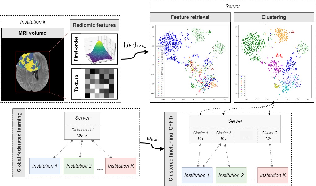
Figure 1: Overall framework of radiomic feature-based clustered federated finetuning.

Formally, let $K$ be the number of institutions, each with a local dataset $D_{k}:=\{(x_{k,i},y_{k,i})\}_{i=1}^{n_{k}}$ with $x_{k,i}\in\mathcal{X}=\mathbb{R}^{m\times h\times w\times d}$ the multimodal MRI scan to segment, $y_{k,i}\in\mathcal{Y}=\{0,1\}^{l\times h\times w\times d}$ its associated multi-label ground-truth segmentation map, $n_{k}$ the local dataset size of institution $k$ and $N=\sum_{k=1}^{K}n_{k}$ the total number of samples. We note $w\in\mathcal{W}=\mathbb{R}^{p}$ the parameters of the neural network to be optimized for the downstream task.

Radiomic features extraction

Each institution extracts a set of radiomic features (first-order and texture features) from each modality and volume. Features of different modalities for a same patient are concatenated into a single feature vector. As opposed to classical approaches with radiomics which try to characterize the texture of a tumor [Shur et al.(2021)Shur, Doran, Kumar, ap Dafydd, Downey, O’Connor, Papanikolaou, Messiou, Koh, and Orton], we compute radiomic features on whole-brain masks on each modality, thus mainly on brain regions which should have a similar appearance with similar acquisition protocols (scanner, parameters, etc.). Formally, for each sample $x_{k,i}$ of institution $k$ a feature vector $f_{k,i}\in\mathbb{R}^{R}$ is computed and transmitted to the server.

Server-side clustering

After retrieving the feature vector associated to each volume of each institution, the server normalizes each feature of each vector. For a given feature with index $r$, we note $f^{r}$ its value in the feature vector $f$. In this study, the chosen normalization follows eq:norm_feature with $P^{r}_{min}$ and $P^{r}_{max}$ being two chosen percentiles on the pooled set of features across all institutions.

$$\hat{f}^{r}_{k,i}=max(0,min(1,\frac{f^{r}_{k,i}-P^{r}_{min}}{P^{r}_{max}-P^{r}_{min}}))$$ (1)

To account for highly correlated features, a principal component analysis (PCA) is applied on the set of normalized feature vectors, followed by the computation of $C$ clusters by fitting a Gaussian mixture model (GMM). For training and inference purpose, the normalization parameters, PCA model and GMM are returned to each institution.
We note $Cluster:\mathbb{R}^{R}\rightarrow\{1,...,C\}$ the application of this clustering process on features extracted from a volume and $\hat{D_{c}}:=\bigcup_{k=1}^{K}\{(x_{k,i},y_{k,i})\ |\ Cluster(\hat{f}_{k,i})=c,\ i\leq n_{k}\}$ the set of samples assigned to cluster $c$ decentralized over the $K$ institutions. We note $n_{c,k}$ the number of samples of institution $k$ assigned to cluster $c$, and $N_{c}=\sum_{k=1}^{K}n_{c,k}$ the total size of $\hat{D}_{c}$.

Global federated learning initialization

Following [McMahan et al.(2017)McMahan, Moore, Ramage, Hampson, and Arcas], we use FedAvg to compute an initial global model $w_{init}$. Given a loss function $l:\mathcal{W}\times\mathcal{X}\times\mathcal{Y}\rightarrow\mathbb{R}$, the classical federated objective can be defined as:

$$w^{*}=\underset{w\in\mathcal{W}}{argmin}\sum_{k=1}^{K}\sum_{i=1}^{n_{k}}l(w,x_{k,i},y_{k,i})\;.$$ (2)

At each communication round $t$, each institution performs $E$ local epoch(s) of stochastic gradient descent (SGD) starting from the current global model $w^{t}$, giving $K$ updates $\Delta w_{k}^{t}=w_{k}^{t}-w^{t}$ to aggregate. The server-side aggregation step is a weighted averaging of these updates $w^{t+1}=w^{t}+\sum_{k=1}^{K}\frac{n_{k}}{N}\Delta w_{k}^{t}$.

Clustered federated finetuning

Given the clustering model computed at server-side, we are now able to define a novel clustered federated learning objective:

$$\{w^{*}_{c}\}_{c=1}^{C}=\underset{\{w_{c}\}_{c=1}^{C}\in\mathcal{W}^{C}}{argmin}\sum_{k=1}^{K}\sum_{i=1}^{n_{k}}l(w_{Cluster(\hat{f}_{k,i})},x_{k,i},y_{k,i})\;,$$ (3)

where $w_{c}$ is the parameter set of the global federated model finetuned on dataset $\hat{D_{c}}$ of cluster $c$. Note that this objective is different from the one defined in recent clustered federated learning approaches such as [Ghosh et al.(2020)Ghosh, Chung, Yin, and Ramchandran] as we compute clusters at sample level, not at institution level, enabling to account for an intra-institution heterogeneity. We optimize each cluster model $w_{c}$ by finetuning the global model $w_{init}$ with FedAvg on the decentralized dataset $\hat{D}_{c}$ for $T_{c}$ rounds. The aggregation step for the federated finetuning of cluster model $w_{c}$ at communication round $t$ becomes $w_{c}^{t+1}=w_{c}^{t}+\sum_{k=1}^{K}\frac{n_{c,k}}{N_{c}}\Delta w_{c,k}^{t}$.

Inference

Given a new sample $x^{\prime}\in\mathcal{X}$ to segment, the whole clustering pipeline is applied to determine which of the $C$ cluster models must be used. That is, radiomic features $f^{\prime}$ are extracted from $x^{\prime}$, normalized following eq:norm_feature, reduced through the computed PCA model, assigned to cluster $c$ using the GMM and segmented with model $w_{c}$.

3 Experiments

3.1 Datasets

Experiments were led using The MICCAI’s Federated Brain Tumor Segmentation 2022 Challenge dataset (FeTS2022) [Bakas et al.(2017)Bakas, Akbari, Sotiras, Bilello, Rozycki, Kirby, Freymann, Farahani, and Davatzikos, Pati et al.(2021)Pati, Baid, Zenk, Edwards, Sheller, Reina, Foley, Gruzdev, Martin, Albarqouni, Chen, Shinohara, Reinke, Zimmerer, Freymann, Kirby, Davatzikos, Colen, Kotrotsou, Marcus, Milchenko, Nazeri, Fathallah-Shaykh, Wiest, Jakab, Weber, Mahajan, Maier-Hein, Kleesiek, Menze, Maier-Hein, and Bakas, Reina et al.(2022)Reina, Gruzdev, Foley, Perepelkina, Sharma, Davidyuk, Trushkin, Radionov, Mokrov, Agapov, Martin, Edwards, Sheller, Pati, Moorthy, Wang, Shah, and Bakas]. This dataset is based on the Brain Tumor Segmentation 2021 Challenge dataset (BraTS2021). Consisting of 1251 multi-modal brain MRI scans (T1, T1ce, T2 and FLAIR) of size $240\times 240\times 155$ with isotropic 1mm³ voxel size along with their multi-label tumor segmentation masks including 3 labels, namely enhancing tumor (ET), tumor core (TC) and whole tumor (WT). The real-world partitioning along the 23 acquiring institutions is provided in addition to the samples, enabling to simulate federated learning. Institutions’ datasets sizes are very heterogeneous (cf Appendix A.1) with $\sim$61% of institutions owning less than 15 samples each. As we do not have the scanner information for every sample, an intra-institution feature shift may exist. This dataset served to evaluate the performance of the proposed clustered federated personalization method and compare it to state-of-the-art methods.

Dataset splitting

In all of the experiments, a $\sim$70-15-15% train - validation - test split was followed, giving 833 training, 218 validation and 200 test samples. We computed such split institution-wise, giving a local training, validation and test dataset per institution. We refer to the global train, validation and test sets as the aggregation of each local set, preserving the representation of each institution in each partition. Due to the computational cost of training models on FeTS2022 and the limited amount of samples ($<5$) provided by multiple institutions, we did not perform cross-validation.

Image volume pre-processing

Each volume was resized to the bounding box containing all brain voxels, padded to a minimum size of 128 on each dimension if necessary. Each modality of each volume’s intensities was then standardized to a zero-mean one-variance gaussian distribution to eliminate the feature shift due to absolute intensity values of scanners.

3.2 Radiomic feature-based clustering

Feature extraction and processing

Ninety-three features including first-order statistics as well as higher order statistical features capturing textural information were extracted per modality using Pyradiomics [van Griethuysen et al.(2017)van Griethuysen, Fedorov, Parmar, Hosny, Aucoin, Narayan, Beets-Tan, Fillion-Robin, Pieper, and Aerts], thus leading to a feature vector of dimension 372. The estimation of these textural features derives from the computation of matrices describing the spatial and intensity relationship between each individual pixel and its neighbors in the image, including GLCM, GLRLM, GLSZM, NGTDM and GLDM [Shur et al.(2021)Shur, Doran, Kumar, ap Dafydd, Downey, O’Connor, Papanikolaou, Messiou, Koh, and Orton]. These matrices require to discretize intensity values of the original images. In this study, we chose an absolute discretization technique based on fixing the histogram bin size to $0.09$ for feature extraction. Features were extracted on whole brain masks. A list of the extracted features is provided in Appendix B.1. We first normalized the feature vectors following eq:norm_feature and setting $P^{r}_{min}$ as the 2nd-centile and $P^{r}_{max}$ as the 98th-centile. Dimension of the normalized feature vectors were then reduced to 30 through PCA, preserving $96.58\%$ of the variance. We validated the radiomic features extraction on The Calgary-Campinas-359 (CC359) dataset (cf Appendix C).

Clustering

We fitted a GMM by setting the number of clusters to 10 on the FeTS2022 samples with tied covariance matrix to account for the limited amount of samples compared to the number of remaining feature dimensions. The performance of the proposed radiomic-based clustering method is assessed visually based on the comparison of 2 t-SNE plots of the radiomic feature distribution where each sample is colored either by the label of its belonging institution or by the label of the cluster it was assigned to through the GMM.

3.3 Clustered federated finetuning (CFFT)

We evaluated the performance of the proposed federated personalization method for the multi-class segmentation task of the FeTS2022 brain MRI dataset based on standard DICE score and 95% Hausdorff distances.

Model architecture and data preprocessing

The backbone architecture used in all experiments is a small-sized 3D U-Net (cf Appendix D) trained on 3D patches of size $128\times 128\times 128$ with a batch size of 1. We used instance normalization without any learned parameters to make the model as robust as possible to any feature shift. If not specified, training includes data augmentation focused on reducing the feature shift (gaussian noise, gaussian smoothing, intensity scaling and gamma contrast adjustment).

Comparison with baseline methods

We validated our approach against different baselines. We first trained a global model on the pooled FeTS2022 dataset (e.g. BraTS2021) with SGD, referred to Centralized in the following. FedAvg was used as the baseline global federated optimization algorithm, as described in sec:fedavg. As a personalized FL baseline, we finetuned the FedAvg final model on each local dataset with SGD; this method is referred to as Local Finetuning. We then experimented with two versions of our CFFT method : the proposed CFFT version preserving the privacy of each clustered dataset $\hat{D}_{c}$ by finetuning with FedAvg and an ideal version referred to as CFFT_ideal, which consists in finetuning on the pooled datasets $\hat{D}_{c}$ of each cluster with SGD.

Training hyperparameters

In Centralized, Local Finetuning and pooled finetuning of CFFT_ideal, a learning rate of 0.02 gave the best results. For federated counterparts, a learning rate of 0.05 was used. A weight decay of $10^{-5}$ was used in all experiments, motivated by state-of-the-art publications [Wang et al.(2020a)Wang, Yurochkin, Sun, Papailiopoulos, and Khazaeni, Yuan et al.(2022)Yuan, Morningstar, Ning, and Singhal]. Centralized training was performed for 300 epochs, FedAvg for 300 communication rounds with one local epoch per round, Local Finetuning for 20 local epochs, CFFT_ideal for 50 epochs and CFFT for 50 communication rounds with one local epoch. The best models at each epoch/communication round were selected based on the validation set performance for all methods. Best results were found by removing data augmentation for clustered finetuning methods, while keeping it for Local Finetuning.

4 Results and Discussion

4.1 Performance of the radiomic features based clustering

We show on fig:t-sne-FeTS2022-inst a t-SNE plot of the radiomic features computed on sample images of FeTS2022. It highlights both inter and intra-institution feature shift in this dataset. We do not have access to the scanner type (vendor, magnetic field) or acquisition parameter to establish further correlation with the observed clusters, but a visual analysis of some example 3D images belonging to different clusters highlights some pattern discrepancies. For example, within institution 4, we can distinguish two types of multi-modal volume appearance (cf Appendix B.2), confirming the existence of intra-institution feature shift, which is well captured by the proposed radiomic based GMM model (fig:t-sne-FeTS2022-cluster). Although out of the scope of this paper, we emphasize that feature normalization enabled to spot some outlier volumes (cf Appendix E).

fig:example2[Colored by institution]   [Colored by GMM cluster]

Figure 2: t-SNE plots of radiomic features computed on FeTS2022 samples.

4.2 Performance of the clustered federated finetuning (CFFT) method

We show in Table 1 and Table 2 aggregated test DICE scores and 95% Hausdorff distances respectively of Centralized, FedAvg, Local Finetuning, CFFT_ideal and CFFT, with sample-wise standard deviation. Per institution results are given in Appendix A.2. On average Centralized training remains the gold standard with the best performance on both metrics. FedAvg produces a less robust model, with a gap of more than one DICE point compared to Centralized on average. This was shown significant based on a two-tailed Wilcoxon signed-rank test for both metrics with $p<0.01$. All personalization methods also significantly improve the FedAvg DICE score in a similar fashion, with CFFT_ideal giving a slight edge on average 95% Hausdorff distance. Note that CFFT_ideal performs better than its federated counterpart CFFT as we could expect. The goal of this preliminary method is to produce clusters of sample with homogeneous appearance and texture. In that sense, the gap on average metrics between CFFT_ideal and CFFT is smaller that between Centralized and FedAvg, motivating a reduction of the shift between institutions taking part in FedAvg in each cluster. Moreover, fig:label_distrib_cluster_fets2022 shows the label distributions of each computed cluster. They are relatively homogeneous, confirming the focus on the feature shift. Other types of shift such as label or concept shifts can be present in the dataset, and we give a hint on their existence in Appendix A.1 with relatively heterogeneous label distributions per institution. Our method’s performance is on par with Local Finetuning while restricting its effect on feature shift. We emphasize that the proposed paradigm of targeting an identified type of shift would potentially generalize better to unseen data.
On a more general note, the choice of the number of clusters is important. Using too few does not capture feature shift, using too many overfits on clustered training data. Ten clusters gave the best validation results. We must acknowledge the relatively high variability of clustering results, possibly due to the high number of dimensions remaining after PCA to preserve sufficient variance. It must also be noted that the high heterogeneity of the local dataset sizes poses problems to assess the performance of personalized methods, with some institutions only owning one or two test samples (cf Appendix A.2). Finally, we hypothesize in this preliminary work that the computed radiomic features are safe to share with a server. We provide a basic validation of the impracticability of reconstructing a volume based on the 93 features extracted per modality in Appendix F, but it remains an open question as to how these features could be leveraged by an attack against our method. Thus, this preliminary work could be improved by studying the compatibility of the framework with known privacy-preserving federated learning techniques such as differential privacy or homomorphic encryption, or developing a federated framework including PCA and clustering. Limiting the amount of computed features to the most relevant ones could also be beneficial while opening explainability opportunities.

Training algorithm	Average	TC	WT	ET
Centralized	0.8912 $\pm$ 0.1201	0.8896 $\pm$ 0.1878	0.9188 $\pm$ 0.0859	0.8651 $\pm$ 0.1956
FedAvg	0.8803 $\pm$ 0.1414	0.8722 $\pm$ 0.2251	0.9099 $\pm$ 0.0906	0.8588 $\pm$ 0.2005
Local finetuning	0.8879 $\pm$ 0.1202	0.8876 $\pm$ 0.1863	0.9132 $\pm$ 0.0891	0.8629 $\pm$ 0.1960
CFFTideal	0.8887 $\pm$ 0.1239	0.8867 $\pm$ 0.1891	0.9139 $\pm$ 0.0892	0.8654 $\pm$ 0.1960
CFFT	0.8874 $\pm$ 0.1254	0.8799 $\pm$ 0.2056	0.9120 $\pm$ 0.0907	0.8704 $\pm$ 0.1852

Table 1: Test DICE scores (mean $\pm$ standard deviation)

Training algorithm	Average	TC	WT	ET
Centralized	5.1348 $\pm$ 6.2212	4.4407 $\pm$ 7.2052	7.0318 $\pm$ 11.0671	3.7770 $\pm$ 8.5314
FedAvg	5.8854 $\pm$ 7.7368	4.7745 $\pm$ 8.0444	8.8814 $\pm$ 15.9499	3.7091 $\pm$ 7.6837
Local finetuning	5.9334 $\pm$ 7.9817	4.8587 $\pm$ 9.3901	8.9284 $\pm$ 16.3270	3.5861 $\pm$ 7.5650
CFFTideal	5.5915 $\pm$ 7.2588	4.6436 $\pm$ 7.3390	8.3688 $\pm$ 15.3738	3.5383 $\pm$ 7.5576
CFFT	5.8749 $\pm$ 7.6108	4.7359 $\pm$ 7.4458	8.8709 $\pm$ 16.4791	3.6520 $\pm$ 7.6291

Table 2: Test 95% Hausdorff distances (mean $\pm$ standard deviation)

fig:label_distrib_cluster_fets2022

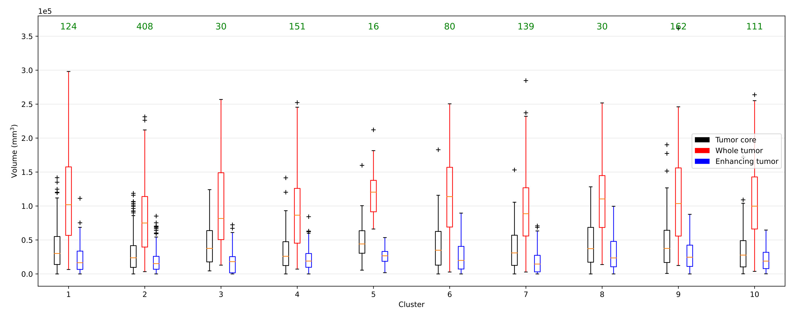
Figure 3: Label distribution per computed cluster in FeTS2022. Green values correspond to the amount of samples associated to each cluster.

This work was partially supported by the Agence Nationale de la Recherche under grant ANR-20-THIA-0007 (IADoc@UdL). It was granted access to the HPC resources of IDRIS under the allocation 2022-AD011013327 made by GENCI.

Appendix A Per institution analysis

A.1 Per institution label distribution and local datasets sizes

fig:label_distrib_inst_fets2022

Figure 4: Label distribution per institution in FeTS2022. Green values correspond to the amount of samples associated to each institution in the complete dataset.

A.2 Per institution results

Institution	Test size	Centralized	FedAvg	Local Finetuning	CFFTideal	CFFT
1	77	0.9300	0.9256	0.9280	0.9289	0.9285
10	2	0.8044	0.8051	0.8076	0.8085	0.8072
11	3	0.9069	0.9000	0.9006	0.9055	0.9053
12	2	0.7386	0.7031	0.7131	0.7032	0.7106
13	6	0.6248	0.4910	0.6090	0.5596	0.5781
14	1	0.6261	0.6115	0.6237	0.6195	0.6100
15	2	0.5924	0.5282	0.6296	0.6135	0.5539
16	5	0.9185	0.9211	0.9265	0.9028	0.9095
17	2	0.9162	0.9133	0.9133	0.9140	0.9101
18	58	0.9187	0.9117	0.9082	0.9138	0.9119
19	1	0.9659	0.9625	0.9634	0.9649	0.9650
2	1	0.9231	0.9221	0.9221	0.9206	0.9160
20	5	0.9386	0.9314	0.9354	0.9346	0.9358
21	6	0.9594	0.9545	0.9559	0.9574	0.9599
22	2	0.9600	0.9553	0.9553	0.9563	0.9570
23	1	0.8881	0.8919	0.8937	0.8879	0.8867
3	3	0.6956	0.5952	0.6946	0.6928	0.6681
4	8	0.6687	0.6669	0.7005	0.6960	0.6943
5	4	0.8057	0.7946	0.7925	0.8349	0.8204
6	6	0.8762	0.8762	0.8762	0.8806	0.8844
7	2	0.8895	0.8873	0.8924	0.8828	0.8804
8	2	0.9631	0.9621	0.9621	0.9645	0.9634
9	1	0.7895	0.8232	0.7818	0.8545	0.8416

Table 3: Average test dice scores per institution

Institution	Test size	Centralized	FedAvg	Local Finetuning	CFFTideal	CFFT
1	77	3.6752	4.3375	4.5268	4.3651	4.4183
10	2	7.5957	7.1775	7.1275	6.8905	7.1512
11	3	3.1412	3.5267	3.2199	3.2042	3.0589
12	2	10.6487	24.9708	26.7511	23.4790	28.9451
13	6	8.1182	12.2476	13.0226	8.0737	10.0930
14	1	3.2863	4.2002	3.3708	4.1926	5.0000
15	2	15.2838	17.3938	18.8894	19.4479	24.4377
16	5	4.3992	8.8826	8.7169	9.8859	9.9735
17	2	1.7756	2.0977	2.0977	1.9249	2.2928
18	58	4.7928	5.1874	5.0459	5.1053	4.8157
19	1	1.6667	1.3333	1.3333	1.1381	1.1381
2	1	5.0726	5.9127	5.9127	6.1498	8.7888
20	5	5.8938	2.6021	2.4663	2.4494	2.3830
21	6	2.1143	2.2983	2.3060	1.6677	1.5816
22	2	2.4694	3.1271	3.1271	3.2594	15.0383
23	1	4.2356	3.9560	3.7742	4.2201	4.2560
3	3	6.5017	9.2293	7.6449	7.4780	8.9391
4	8	14.1589	12.5674	12.6770	10.3157	10.3217
5	4	5.2451	7.8477	7.7993	6.7148	7.6399
6	6	10.0190	10.2264	10.2264	9.6674	9.5711
7	2	12.2938	15.7393	14.9248	16.0055	16.4357
8	2	1.2761	1.4267	1.4267	1.3291	1.3738
9	1	12.8816	6.7070	7.9211	6.1545	6.5459

Table 4: Average test hausdorff distances per institution

Appendix B Radiomic features extraction

B.1 Radiomic features list

Using Pyradiomics, 93 features are extracted per modality:

• First Order Statistics (18 features) (standard deviation is not included)

• Gray Level Cooccurence Matrix (GLCM) (24 features)

• Gray Level Run Length Matrix (GLRLM) (16 features)

• Gray Level Size Zone Matrix (GLSZM) (16 features)

• Neighbouring Gray Tone Difference Matrix (NGTDM) (5 features)

• Gray Level Dependence Matrix (GLDM) (14 features)

B.2 Visual examples

fig:visual_example_01172

Figure 5: FeTS2022_01172 MRI scans, owned by institution 4, assigned to cluster 7.

fig:visual_example_01195

Figure 6: FeTS2022_01195 MRI scans, owned by institution 4, assigned to cluster 4.

Appendix C Radiomic features validation on CC359

Dataset

The Calgary-Campinas-359 (CC359) dataset [Souza et al.(2018)Souza, Lucena, Garrafa, Gobbi, Saluzzi, Appenzeller, Rittner, Frayne, and Lotufo]. This dataset consists of 359 T1-weighted brain MRI scans of healthy subjects along with their ”silver-standards” brain masks generated both using the STAPLE algorithm. These images were acquired on scanners from three vendors (Siemens, Philips and General Electric) at both 1.5 T and 3 T. Sixty exams were acquired per vendor and magnetic field strength, except for Philips 1.5T which totalizes 59 exams. This dataset, concatenating 6 series of exams of equal size and low intra-feature shift serves as a use case to validate the radiomic feature extraction process.

Parameters

We fixed the histogram bin size to $0.15$ for features extraction on the CC359 dataset. We normalized the feature vectors following eq:norm_feature and setting $P^{r}_{min}$ as the 2nd-centile and $P^{r}_{max}$ as the 98th-centile. Dimension of the normalized feature vectors is then reduced to 30 through PCA, preserving $99.96\%$ of the variance.

Results

We show on fig:t-sne-cc359 a t-SNE plot of the radiomic features computed on CC359 after normalization and PCA where each label encodes for one of the 6 scanners on which the image were acquired (e.g. philips_3 corresponds to a 3T Philips scanner). Despite only dealing with healthy patients with a normalization process that significantly reduces feature shift, distinct clusters can be identified for each scanner manufacturer and magnetic field value. This demonstrates the capacity of the selected radiomic feature vector to capture textural patterns induced by the scanner characteristics.

fig:t-sne-cc359

Figure 7: t-SNE of radiomic features.

Appendix D Model architecture

We use a small-sized 3D U-Net as the backbone architecture. It includes 3 down-sampling and up-sampling paths. Stride 2 convolutions are used in down-sampling paths, and transpose convolutions for up-sampling paths. Kernel size is (3,3,3) for every convolution block. A first stride 1 convolution block outputs 16 channels, multiplied by 2 at each downsampling path to reach 128 channels in the bottleneck part of the network. Inference are done with a sliding window with an overlap of 0.5 and Gaussian aggregation of results on overlaps.

Appendix E Outliers detection

For some extracted features, the normalization process clearly highlighted outliers. As example, the GLCM Cluster Prominence feature computed on the FLAIR n°1441 was two orders of magnitude higher than for any other volume. We verified that this volume has a particular appearance, with extreme intensities toward the eye balls (fig:flair-1441). Such manually computed features can thus be leveraged for federated outlier detection without sacrificing too much privacy.

fig:flair-1441

Figure 8: Flair MRI scan of patient n°1441

Appendix F Privacy preservation basic validation

We explore in this section the efficiency of an attack on the radiomic features communicated during the proposed clustered federated finetuning process. Its objective is, given every normalized feature vector computed on the train and validation T1 volumes, to train a decoder to reconstruct the associated volumes. Each volume was standardized and resized to $128^{3}$ voxels to simplify the task.

Model

The model is composed of a first linear layer outputting 4096 values reshaped to [512, 2, 2, 2], followed by 6 3D residual convolutional blocks, upsampling each dimension by a factor of 2 while dividing the number of channels by 2. We use 3D batch normalization and LeakyRelu activation function with a slope of 0.2 between each layer. The model is composed of approximately 20 millions parameters.

Training parameters

We train this model using the same training - validation - test split as for the original segmentation task. The loss and metric used is a standard MSE. We use Adam with a learning rate of 1e-4 and a weight decay of 1e-5 for 300 epochs with a batch size of 2. The final model is selected based on best validation performance.

Result

We show in fig:privacy_loss_plot the training and validation loss curves. After only 20 epochs, the model starts to overfit on the training set with a stagnating validation performance. We show in fig:privacy_example two slices of reconstruction outputs of the test set. The model is only able to reconstruct an average volume, validating the fact that the transmitted feature vectors do not contain enough information to reconstruct a volume, even the tumorous parts. The proposed scheme of attack is also unrealistically powerful, as it presumes a large amount of already leaked data.

fig:privacy_loss_plot

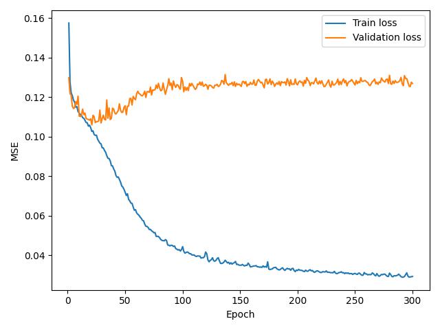
Figure 9: Training and validation loss curves of a model reconstructing T1 volumes based on extracted radiomic features.

fig:privacy_example[T1 scan of patient n°176]   [T1 scan of patient n°134]

Figure 10: Example outputs of a model trained to reconstruct T1 volumes based on transmitted radiomic features. We show slice n°64 for both samples. On the left are ground truth standardized volumes, on the right are reconstructed volumes.

References

- [Acar et al.(2021)Acar, Zhao, Zhu, Matas, Mattina, Whatmough, and Saligrama] Durmus Alp Emre Acar, Yue Zhao, Ruizhao Zhu, Ramon Matas, Matthew Mattina, Paul Whatmough, and Venkatesh Saligrama. Debiasing Model Updates for Improving Personalized Federated Training. In Proceedings of the 38th International Conference on Machine Learning, July 2021.
- [Arivazhagan et al.(2019)Arivazhagan, Aggarwal, Singh, and Choudhary] Manoj Ghuhan Arivazhagan, Vinay Aggarwal, Aaditya Kumar Singh, and Sunav Choudhary. Federated Learning with Personalization Layers. arXiv:1912.00818 [cs, stat], December 2019.
- [Bakas et al.(2017)Bakas, Akbari, Sotiras, Bilello, Rozycki, Kirby, Freymann, Farahani, and Davatzikos] Spyridon Bakas, Hamed Akbari, Aristeidis Sotiras, Michel Bilello, Martin Rozycki, Justin S. Kirby, John B. Freymann, Keyvan Farahani, and Christos Davatzikos. Advancing The Cancer Genome Atlas glioma MRI collections with expert segmentation labels and radiomic features. Scientific Data, 4(1), September 2017.
- [Fallah et al.(2020)Fallah, Mokhtari, and Ozdaglar] Alireza Fallah, Aryan Mokhtari, and Asuman Ozdaglar. Personalized Federated Learning with Theoretical Guarantees: A Model-Agnostic Meta-Learning Approach. In Advances in Neural Information Processing Systems, volume 33, 2020.
- [Futrega et al.(2022)Futrega, Milesi, Marcinkiewicz, and Ribalta] Michał Futrega, Alexandre Milesi, Michał Marcinkiewicz, and Pablo Ribalta. Optimized U-Net for Brain Tumor Segmentation. In Alessandro Crimi and Spyridon Bakas, editors, Brainlesion: Glioma, Multiple Sclerosis, Stroke and Traumatic Brain Injuries, Lecture Notes in Computer Science, 2022.
- [Ghosh et al.(2020)Ghosh, Chung, Yin, and Ramchandran] Avishek Ghosh, Jichan Chung, Dong Yin, and Kannan Ramchandran. An efficient framework for clustered federated learning. In Proceedings of the 34th International Conference on Neural Information Processing Systems, NIPS’20, December 2020.
- [Karimireddy et al.(2020)Karimireddy, Kale, Mohri, Reddi, Stich, and Suresh] Sai Praneeth Karimireddy, Satyen Kale, Mehryar Mohri, Sashank Reddi, Sebastian Stich, and Ananda Theertha Suresh. SCAFFOLD: Stochastic Controlled Averaging for Federated Learning. In International Conference on Machine Learning, November 2020.
- [Li et al.(2020)Li, Sahu, Zaheer, Sanjabi, Talwalkar, and Smith] Tian Li, Anit Kumar Sahu, Manzil Zaheer, Maziar Sanjabi, Ameet Talwalkar, and Virginia Smith. Federated Optimization in Heterogeneous Networks, April 2020.
- [Li et al.(2021)Li, Hu, Beirami, and Smith] Tian Li, Shengyuan Hu, Ahmad Beirami, and Virginia Smith. Ditto: Fair and Robust Federated Learning Through Personalization. In Proceedings of the 38th International Conference on Machine Learning, July 2021.
- [Li et al.(2019)Li, Milletarì, Xu, Rieke, Hancox, Zhu, Baust, Cheng, Ourselin, Cardoso, and Feng] Wenqi Li, Fausto Milletarì, Daguang Xu, Nicola Rieke, Jonny Hancox, Wentao Zhu, Maximilian Baust, Yan Cheng, Sébastien Ourselin, M. Jorge Cardoso, and Andrew Feng. Privacy-Preserving Federated Brain Tumour Segmentation. In Heung-Il Suk, Mingxia Liu, Pingkun Yan, and Chunfeng Lian, editors, Machine Learning in Medical Imaging, Lecture Notes in Computer Science, 2019.
- [Liu et al.(2021a)Liu, Chen, Qin, Dou, and Heng] Quande Liu, Cheng Chen, Jing Qin, Qi Dou, and Pheng-Ann Heng. FedDG: Federated Domain Generalization on Medical Image Segmentation via Episodic Learning in Continuous Frequency Space. In 2021 IEEE/CVF Conference on Computer Vision and Pattern Recognition (CVPR), June 2021a.
- [Liu et al.(2021b)Liu, Song, Liu, and Zhang] Xiangbin Liu, Liping Song, Shuai Liu, and Yudong Zhang. A Review of Deep-Learning-Based Medical Image Segmentation Methods. Sustainability, 13(3), January 2021b.
- [Marfoq et al.(2021)Marfoq, Neglia, Bellet, Kameni, and Vidal] Othmane Marfoq, Giovanni Neglia, Aurélien Bellet, Laetitia Kameni, and Richard Vidal. Federated Multi-Task Learning under a Mixture of Distributions. In Advances in Neural Information Processing Systems, volume 34, 2021.
- [McMahan et al.(2017)McMahan, Moore, Ramage, Hampson, and Arcas] Brendan McMahan, Eider Moore, Daniel Ramage, Seth Hampson, and Blaise Aguera y Arcas. Communication-Efficient Learning of Deep Networks from Decentralized Data. In Artificial Intelligence and Statistics, April 2017.
- [Pati et al.(2021)Pati, Baid, Zenk, Edwards, Sheller, Reina, Foley, Gruzdev, Martin, Albarqouni, Chen, Shinohara, Reinke, Zimmerer, Freymann, Kirby, Davatzikos, Colen, Kotrotsou, Marcus, Milchenko, Nazeri, Fathallah-Shaykh, Wiest, Jakab, Weber, Mahajan, Maier-Hein, Kleesiek, Menze, Maier-Hein, and Bakas] Sarthak Pati, Ujjwal Baid, Maximilian Zenk, Brandon Edwards, Micah Sheller, G. Anthony Reina, Patrick Foley, Alexey Gruzdev, Jason Martin, Shadi Albarqouni, Yong Chen, Russell Taki Shinohara, Annika Reinke, David Zimmerer, John B. Freymann, Justin S. Kirby, Christos Davatzikos, Rivka R. Colen, Aikaterini Kotrotsou, Daniel Marcus, Mikhail Milchenko, Arash Nazeri, Hassan Fathallah-Shaykh, Roland Wiest, Andras Jakab, Marc-Andre Weber, Abhishek Mahajan, Lena Maier-Hein, Jens Kleesiek, Bjoern Menze, Klaus Maier-Hein, and Spyridon Bakas. The Federated Tumor Segmentation (FeTS) Challenge. arXiv:2105.05874 [cs, eess], May 2021.
- [Pillutla et al.(2022)Pillutla, Malik, Mohamed, Rabbat, Sanjabi, and Xiao] Krishna Pillutla, Kshitiz Malik, Abdel-Rahman Mohamed, Mike Rabbat, Maziar Sanjabi, and Lin Xiao. Federated Learning with Partial Model Personalization. In Proceedings of the 39th International Conference on Machine Learning, June 2022.
- [Reina et al.(2022)Reina, Gruzdev, Foley, Perepelkina, Sharma, Davidyuk, Trushkin, Radionov, Mokrov, Agapov, Martin, Edwards, Sheller, Pati, Moorthy, Wang, Shah, and Bakas] G. Anthony Reina, Alexey Gruzdev, Patrick Foley, Olga Perepelkina, Mansi Sharma, Igor Davidyuk, Ilya Trushkin, Maksim Radionov, Aleksandr Mokrov, Dmitry Agapov, Jason Martin, Brandon Edwards, Micah J. Sheller, Sarthak Pati, Prakash Narayana Moorthy, Shih-han Wang, Prashant Shah, and Spyridon Bakas. OpenFL: An open-source framework for Federated Learning. Physics in Medicine & Biology, 67(21), November 2022.
- [Sattler et al.(2021)Sattler, Müller, and Samek] Felix Sattler, Klaus-Robert Müller, and Wojciech Samek. Clustered Federated Learning: Model-Agnostic Distributed Multitask Optimization Under Privacy Constraints. IEEE Transactions on Neural Networks and Learning Systems, 32(8), August 2021.
- [Shamsian et al.(2021)Shamsian, Navon, Fetaya, and Chechik] Aviv Shamsian, Aviv Navon, Ethan Fetaya, and Gal Chechik. Personalized Federated Learning using Hypernetworks. In Proceedings of the 38th International Conference on Machine Learning, July 2021.
- [Shur et al.(2021)Shur, Doran, Kumar, ap Dafydd, Downey, O’Connor, Papanikolaou, Messiou, Koh, and Orton] Joshua D. Shur, Simon J. Doran, Santosh Kumar, Derfel ap Dafydd, Kate Downey, James P. B. O’Connor, Nikolaos Papanikolaou, Christina Messiou, Dow-Mu Koh, and Matthew R. Orton. Radiomics in oncology: A practical guide. RadioGraphics, 41(6), 2021.
- [Souza et al.(2018)Souza, Lucena, Garrafa, Gobbi, Saluzzi, Appenzeller, Rittner, Frayne, and Lotufo] Roberto Souza, Oeslle Lucena, Julia Garrafa, David Gobbi, Marina Saluzzi, Simone Appenzeller, Letícia Rittner, Richard Frayne, and Roberto Lotufo. An open, multi-vendor, multi-field-strength brain MR dataset and analysis of publicly available skull stripping methods agreement. NeuroImage, 170, April 2018.
- [Tang et al.(2022)Tang, Zhang, Shi, He, Han, and Chu] Zhenheng Tang, Yonggang Zhang, Shaohuai Shi, Xin He, Bo Han, and Xiaowen Chu. Virtual Homogeneity Learning: Defending against Data Heterogeneity in Federated Learning. In Proceedings of the 39th International Conference on Machine Learning, June 2022.
- [van Griethuysen et al.(2017)van Griethuysen, Fedorov, Parmar, Hosny, Aucoin, Narayan, Beets-Tan, Fillion-Robin, Pieper, and Aerts] Joost J. M. van Griethuysen, Andriy Fedorov, Chintan Parmar, Ahmed Hosny, Nicole Aucoin, Vivek Narayan, Regina G. H. Beets-Tan, Jean-Christophe Fillion-Robin, Steve Pieper, and Hugo J. W. L. Aerts. Computational Radiomics System to Decode the Radiographic Phenotype. Cancer Research, 77(21), November 2017.
- [Wang et al.(2020a)Wang, Yurochkin, Sun, Papailiopoulos, and Khazaeni] Hongyi Wang, Mikhail Yurochkin, Yuekai Sun, Dimitris Papailiopoulos, and Yasaman Khazaeni. Federated learning with matched averaging. In International Conference on Learning Representations, 2020a.
- [Wang et al.(2020b)Wang, Liu, Liang, Joshi, and Poor] Jianyu Wang, Qinghua Liu, Hao Liang, Gauri Joshi, and H. Vincent Poor. Tackling the Objective Inconsistency Problem in Heterogeneous Federated Optimization. In Advances in Neural Information Processing Systems, volume 33, 2020b.
- [Xu et al.(2022)Xu, Li, Guo, Yang, Roth, Hatamizadeh, Zhao, Xu, Huang, and Xu] A. Xu, W. Li, P. Guo, D. Yang, H. Roth, A. Hatamizadeh, C. Zhao, D. Xu, H. Huang, and Z. Xu. Closing the generalization gap of cross-silo federated medical image segmentation. In 2022 IEEE/CVF Conference on Computer Vision and Pattern Recognition (CVPR), jun 2022.
- [Yu et al.(2022)Yu, Bagdasaryan, and Shmatikov] Tao Yu, Eugene Bagdasaryan, and Vitaly Shmatikov. Salvaging Federated Learning by Local Adaptation, March 2022.
- [Yuan et al.(2022)Yuan, Morningstar, Ning, and Singhal] Honglin Yuan, Warren Richard Morningstar, Lin Ning, and Karan Singhal. What do we mean by generalization in federated learning? In International Conference on Learning Representations, 2022.