Robust-MBFD: A Robust Deep Learning System for Motor
Bearing Faults Detection Using Multiple Deep Learning
Training Strategies and A Novel Double Loss Function

Abstract

This paper presents a comprehensive analysis of motor bearing fault detection (MBFD), which involves the task of identifying faults in a motor bearing based on its vibration. To this end, we first propose and evaluate various machine learning based systems for the MBFD task. Furthermore, we propose three deep learning based systems for the MBFD task, each of which explores one of the following training strategies: supervised learning, semi-supervised learning, and unsupervised learning. The proposed machine learning based systems and deep learning based systems are evaluated, compared, and then they are used to identify the best model for the MBFD task. We conducted extensive experiments on various benchmark datasets of motor bearing faults, including those from the American Society for Mechanical Failure Prevention Technology (MFPT), Case Western Reserve University Bearing Center (CWRU), and the Condition Monitoring of Bearing Damage in Electromechanical Drive Systems from Paderborn University (PU). The experimental results on different datasets highlight two main contributions of this study. First, we prove that deep learning based systems are more effective than machine learning based systems for the MBFD task. Second, we achieve a robust and general deep learning based system with a novel loss function for the MBFD task on several benchmark datasets, demonstrating its potential for real-life MBFD applications.

Keywords— Acoustic scene classification, ensemble, feature extraction, back-end deep neural network, embeddings, back-bone convolution neural network, multi spectrograms.

I Introduction

The statistics in [1] and [2] indicate that rolling bearing damages occupy from 40% to 70% of electro-mechanic drive systems and motor failures, leading to significantly high costs for motor-based systems. To address this issue, the maintenance process, capable of automatically detecting motor bearing faults, requires continuous monitoring. The most common method for monitoring motor bearing faults involves analyzing vibration data collected from acceleration sensors integrated into motors. Recently, the analysis of vibration data for detecting motor bearing damages has garnered significant research attention and has yielded promising results through the application of machine learning and deep learning based models.

For the motor bearing faults detection (MBFD) task, machine learning based systems leverage vibration input data and initially extract features from both the time and frequency domains. For instance, time domain features such as mean, root mean square (RMS), kurtosis, peak-to-peak, variance (Var), standard deviation (SD), shape factor, peaking factor, pulse factor, and margin factor are widely utilized [3, 4, 5]. Simultaneously, statistical features like root mean square frequency (RMSF), center frequency (CF), mean square frequency (MSF), frequency variance (VF), and root frequency variance (RVF) from the frequency domain are commonly extracted [6, 7]. These features from different domains are concatenated to create a multi-domain-based feature, often referred to as hand-crafted features. Given the wide range of features extracted from different domains, some features lack distinctiveness among damage categories, leading to decreased classification model performance. To address this issue, researchers have proposed various methods to analyze hand-crafted features, identifying which features are more significant and subsequently removing non-significant ones. For example, Nayana and Geethanjali in [8] initially extracted 18 statistical features from both the time and frequency domains. They then applied wheel-based differential evolution (WBDE) and particle swarm optimization (PSO) methods to process, rank, and remove non-significant features. Meanwhile, Yue et al. in [9] utilized principal component analysis (PCA) to reduce feature dimensionality before inputting the data into a classification model. To further enhance hand-crafted features, some researchers have proposed applying entropy to characterize the uncertainty of these features. For instance, Dongfang et al.[10] focused on improving the scale factor of multi-scale entropy to address the issue of insufficient accuracy. Similarly, Keheng et al.[11] introduced a method to calculate hierarchical entropy of vibration signals, generating hierarchical-entropy-based features. To classify the hand-crafted features into target categories, a wide range of traditional machine learning methods, such as support vector machines (SVM)[12, 13], k-Nearest Neighbor (kNN)[14, 15], and naive Bayes [16], are applied. To further boost performance, ensemble methods have been proposed, such as applying the Adaboost algorithm to SVM models in [17], or using an ensemble of multiple classifiers [18].

Concerning deep learning based systems used for the MBFD task, a wide range of deep neural network architectures, such as autoencoder-based networks [19, 20, 21], Convolutional Neural Networks (CNN)[22, 23, 24, 25], generative adversarial networks[26, 27], recurrent neural networks (RNN)[28, 20], or combinations of CNN and RNN[29, 30, 31], have been proposed. Among these deep neural networks, CNN-based network architectures have gained popularity. These CNN-based networks are designed to directly learn input signals without the need for extracting hand-crafted features as in machine learning based systems. To further enhance performance, some researchers [32, 33] have applied various transfer learning techniques to CNN-based network architectures. For instance, in [32], the pre-trained ResNet-50 network on ImageNet [34] serves as the backbone for extracting feature maps. In contrast, authors in [33] initially trained an MLP-based network architecture on a bearing fault dataset (source data) and then adapted this pre-trained MLP-based model for training on another bearing fault dataset (target data).

Upon reviewing the recent systems mentioned above, several observations can be seen: (I) The state-of-the-art systems utilize either machine learning or deep learning based models for the MBFD task. However, none of the research has proposed a comprehensive analysis and comparison between these two approaches. (II) Additionally, the state-of-the-art machine learning and deep learning based systems for the MBFD task predominantly employ the supervised learning strategy to train classification models. Meanwhile, none of the papers have explored semi-supervised or unsupervised training methods to evaluate the MBFD task. (III) Finally, the currently proposed MBFD systems evaluate various datasets using different training-testing splitting methods, making it challenging to compare the performance among proposed network architectures. For example, although the Paderborn University (PU) dataset [18] currently presents the largest dataset of motor bearing damages and also suggests official splitting methods [35], the proposed MBFD systems evaluating this dataset suggest their own splitting methods. In this paper, we aim to address the existing gaps in MBFD research and make the following main contributions:

1. Firstly, we introduce not only machine learning but also deep learning based systems for the MBFD task. Our experimental results for both approaches indicate that deep learning based methods are more effective.
   

2. To explore deep learning based systems, we propose three different deep learning models, each of which is trained with specific strategies: supervised learning, semi-supervised learning, and unsupervised learning, respectively. We then leverage three proposed deep learning architectures and different training strategies to develop a robust deep learning model for MBFD, referred to as the Robust-MBFD. To train the Robust-MBFD model, we proposed a novel loss function, namely Double loss, which presents a combination of Triplet loss and Center loss.
   

3. Finally, we evaluate the performance of the best model on several benchmark datasets, including the American Society for Mechanical Failure Prevention Technology (MFPT) [36], Case Western Reserve University Bearing Center (CWRU) [37], and Condition Monitoring of Bearing Damage in Electromechanical Drive Systems from Paderborn University (PU) [18]. For each dataset, we provide detailed descriptions of different training/testing splitting methods, which can be considered official benchmarks for comparing proposed MBFD systems. Our experimental results on diverse datasets with various splitting settings demonstrate the robustness and generality of our best model across different MBFD datasets.

II Machine learning and deep learning based systems for bearing fault detection

In this paper, we propose two approaches to develop a system for motor bearing fault detection (MBFD), which is based on (1) machine learning and (2) deep learning techniques.

II-A Proposed machine learning based systems

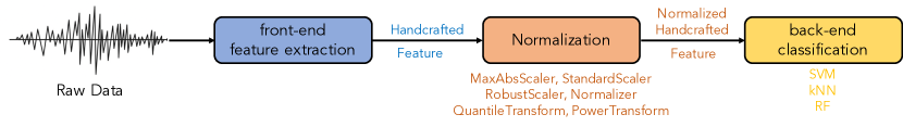
Figure 1: The high-level architecture of the machine learning based systems.

TABLE I: Back-end machine learning based classification models and setting parameters.

Machine Learning Models	Setting Parameters
Support Vector Machine (SVM)	C=1.0
	kernel=‘RBF’
	gamma=‘scale’
K-Nearest Neighbors (kNN)	n_neighbors = 5
	weights = ’uniform’
	leaf_size 30
	p=2
Random Forest (RF)	max depth of tree = 20,
	number of trees = 100

The high-level architecture of our proposed machine learning based systems is presented in Fig. 1. As Fig. 1 shows, the machine learning based systems comprise three main parts: Front-end feature extraction, normalizarion, and back-end classification model.

Front-end feature extraction: First, both time-domain features and frequency-domain features are extracted from the raw data. Concerning the time-domain features, we extract root mean square (RMS), variance (Var), peak values, kurtosis, skewness, peak-to-peak value, line integral, and four factor values (crest factor, clearance factor, impulse factor, shape factor), which are inspired by [38]. In the frequency domain, we extract the spectral centroid, spectral bandwidth, spectral flatness, and roll-off frequency, which are inspired by [39]. The time-domain and frequency-domain features are then concatenated to create combined features representing input vibration data, referred to as the hand-crafted features.

Normalization: The hand-crafted features are then normalized using various normalization methods: max absolute scaler (MAS), standard scaler (SS), robust scaler (RS), normalization (Norm), quantile transformer (QT), and power transformer (PT), which are inspired by [40].

Back-end classification model: To classify the normlaized hand-crafted features, we evaluate various machine learning based models: Support Vector Machine (SVM), k-nearest neighbors (kNN), and Random Forest (RF). The settings for each machine learning method are presented in Table I.

II-B Proposed deep learning based systems

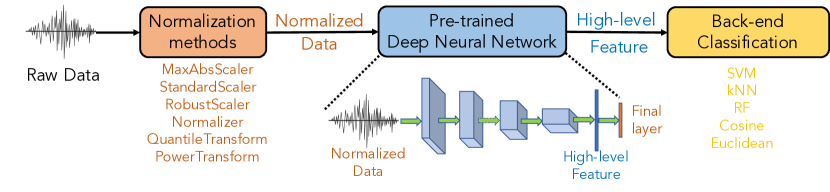
Figure 2: The high-level architecture of the deep learning based systems.

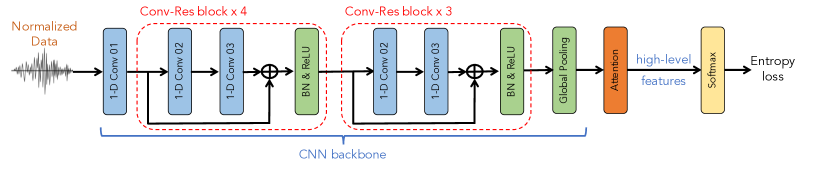
Figure 3: The architecture of the supervised deep learning model (SDLM).

The high-level architecture of our proposed deep learning based systems is shown in Fig. 2. As described in Fig. 2, the proposed deep learning based systems comprise three main components: Normalization, high-level feature extraction, and back-end classification in the order.

Normalization: These methods, designed to normalize the raw vibration data, are reused from the machine learning based systems presented in Section II-A.

High-level feature extraction: The normalized vibration input data is subsequently input into a deep neural network for training. After the training process, the normalized data is again passed through the pre-trained network to extract feature maps, which constitute the output of the final fully connected layer as shown in the lower part of Fig. 2. These feature maps are referred to as the high-level features.

Back-end classification: The high-level features are then classified into specific classes using machine learning based models such as support vector machines (SVM), k-nearest neighbors (kNN), random forest (RF) mentioned in Section II-A, as well as Euclidean and Cosine distance measurement methods.

Compare between the high-level architecture of machine learning and deep learning based systems, it’s evident that these two approaches differ primarily in the feature extraction step. In the case of machine learning based systems, hand-crafted features are extracted in both the time and frequency domains. In contrast, deep learning based systems leverage deep neural networks to directly train the normalized input data without the need for extracting hand-crafted features. Subsequently, feature maps from the networks are utilized to derive the high-level features.

II-C Proposed deep neural network architectures to extract the high-level features

In this paper, we propose three types of deep neural network architectures for extracting high-level features. The first deep neural network architecture is illustrated in Fig.3. As shown in Fig.3, the proposed network architecture consists of four main components: one 1-dimensional convolutional block (1-D Conv 01), followed by two convolutional-residual blocks (Conv-Res), and finally, one attention block (Attention). The two convolutional-residual blocks share the same architecture, each of which includes two 1-D convolutional sub-blocks: 1-D Conv 02 and 1-D Conv 03, followed by batch normalization (BN)[41] and rectified linear unit (ReLU)[42]. The detailed configuration of the 1-D Conv 01, 1-D Conv 02, and 1-D Conv 03 blocks is provided in Table II.

TABLE II: Configuration of Convolutional and Attention blocks

Blocks	Layers
1-D Conv 01	Conv[$48\times 80$] - BN - ReLU - MP[$4$]
1-D Conv 02	Conv[$48\times 3$] - BN - ReLU
1-D Conv 03	Conv[$96\times 3$] - BN
Attention	Head=4, Key-Dimension=48

The output of the Conv-Res blocks is passed through a Global Average Pooling (GAP) layer, followed by an Attention layer. The attention layer employs a Multihead attention scheme, empirically configured with 4 heads and a key dimension of 48, as illustrated in Table II. Finally, a Softmax layer computes the predicted probabilities for specific classes. As we utilize the Cross-Entropy loss, as shown in Equation (1), to compare the predicted probabilities (i.e., the output of the Softmax layer) $\hat{\mathbf{y}}$ with the true labels $\mathbf{y}$, we refer to this network as the supervised deep learning model (SDLM).

$$\mathcal{L}_{entropy}=-\sum_{i}y_{i}\cdot\log(\hat{y}_{i})$$ (1)

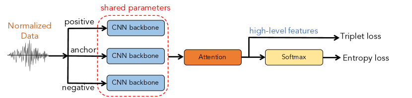
Figure 4: The architecture of the semi-supervised deep learning model (S-SDLM).

The second deep neural network reuses the supervised deep learning architecture mentioned earlier. Specifically, we consider the first layer up to the global pooling layer of the SDLM model in Fig.3 as the convolutional neural network backbone (CNN-based backbone). With the CNN-based backbone in place, we construct a triplet-based network architecture, sharing the CNN-based backbone, to learn from three types of inputs: anchor, positive, and negative data, as illustrated in Fig.4. The output feature map from the CNN backbone is then used in two loss functions. The first loss function, employing Cross-Entropy, assists in classifying the embeddings into specific classes as Equation (1). Meanwhile, the second loss, known as the Triplet loss [43], aims to increase the distances between the negative embeddings and the group of positive and anchor embeddings. If we consider the input data vectors $\mathbf{X}$ as embedding vectors obtained after passing through the CNN-based backbone, the Triplet loss proposed is defined by:

$$H_{i}=d^{2}(\mathbf{X}^{a}_{i},\mathbf{X}^{p}_{i})-d^{2}(\mathbf{X}^{a}_{i},\mathbf{X}^{n}_{i})+m$$ (2)

$$\mathcal{L}_{triplet}=\underset{\theta\in\mathbb{R}}{\text{argmin}}\sum_{i=1}^{n}\max(H_{i},0)$$ (3)

where $\mathbf{X}^{a}_{i}$, $\mathbf{X}^{p}_{i}$, and $\mathbf{X}^{n}_{i}$ represent embedding vectors from anchor, positive, and negative samples, respectively, where $i$ denotes the index for each number of training samples (batch size). The Euclidean distance [44] between embedding vectors from anchor and positive is denoted by $d^{2}(\mathbf{X}^{a}_{i},\mathbf{X}^{p}_{i})$, and $d^{2}(\mathbf{X}^{a}_{i},\mathbf{X}^{n}_{i})$ for the Euclidean distance between embedding vectors from anchor and negative. Additionally, $m$ represents a margin value used to enforce a minimum distance between positive pairs and negative pairs. The final loss function for training the proposed model, which combines the Cross-Entropy loss and Triplet loss, is described as follows:

$$\mathcal{L}_{S-SDML}=\mathcal{L}_{triplet}+\lambda\mathcal{L}_{entropy}$$ (4)

As we use two loss functions of Cross-Entropy and Triplet, we refer the second deep neural network to as the semi-supervised deep learning model (S-SDLM).

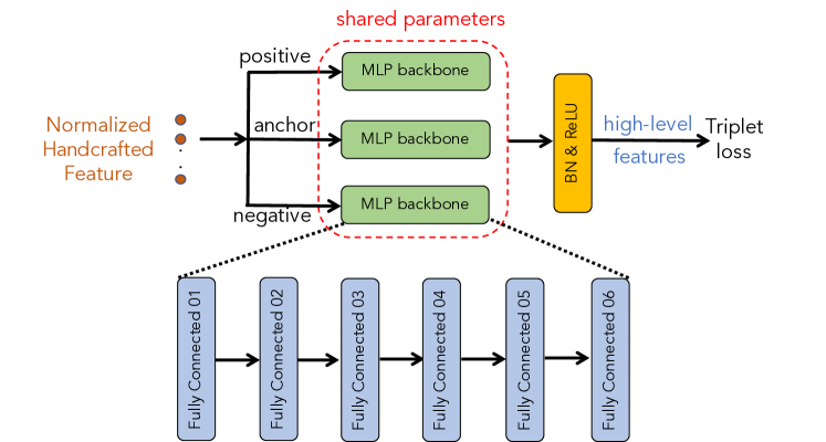
Figure 5: The architecture of the un-supervised deep learning model (U-SDLM).

The third deep neural network also leverages the triplet network architecture, as shown in Fig.5. The input of the triplet network architecture consists of the hand-crafted features used in the machine learning based models in Section II-A. However, the backbone used in this network architecture employs a multilayer perceptron (MLP) architecture, referred to as the MLP-based backbone, comprising six fully connected layers with kernel sizes of 1024, 512, 128, 512, 1024, and 256, respectively. Since we utilize only one Triplet loss function to learn the feature map output of the MLP-based backbone, we refer to this network architecture as the unsupervised deep learning model (U-SDLM). Regarding the Triplet loss, it is expressed as Equation (2) and Equation (3).

For the SDLM and S-SDLM models, the feature map output of Attention block is considered as the high-level features. Meanwhile, the feature map output of MLP-based backbone in U-SDLM is referred to as the high-level feature. After training these three models, high-level features are extracted from SDLM, S-SDLM, and U-SDLM models to feed into traditional machine learning models (e.g. SVM, RF, kNN) or distance-based methods (e.g.Cosine and Euclidian distances) for classification as mentioned in Fig. 2.

To evaluate our proposed models, we conduct experiments on three benchmark datasets of bearing vibration: The first dataset of PU Bearing [18] dataset comprises both artificial and real damaged bearings; Two other datasets of CWRU Bearing [37] and MFPT bearing [36] present artificial damaged bearings.

TABLE III: Evaluating setup of PU Bearing dataset with training on artificial data and test on real data (PU-C1)

Class		Training	Testing
1	Healthy	K002	K001
2	OR Damage	KA01	KA22
		KA05	KA04
		KA07	KA15
			KA30
			KA16
3	IR Damage	KI01	KI14
		KI05	KI21
		KI07	KI17
			KI18
			KI16

TABLE IV: Evaluating setup of PU Bearing dataset with training and testing on real data (PU-C2)

Healthy	Outer Ring Damages	Inner Ring Damages
K001	KA04	KI04
K002	KA15	KI14
K003	KA16	KI16
K004	KA22	KI18
K005	KA30	KI21

III Experimental Settings

PU Bearing [18]: The bearing dataset, which was published by Paderborn University, currently presents the largest dataset of vibration data proposed for detecting damage in motors’ bearings. There are a total of 32 different bearings used to collect vibration data in this dataset: 12 bearings with artificial damages (i.e., These bearings, named KA01, KA03, KA05, KA06, KA07, KA08, and KA09, are for outer ring damages; The bearings KI01, KI03, KI05, KI07, and KI08 are marked for inner ring damages), 14 real damaged bearings collected from accelerated lifetime tests (i.e., The bearings KA04, KA15, KA16, KA22, KA30 are for outer ring damages; Inner ring damaged bearings are named KI04, KI14, KI16, KI17, KI18, KI21; The remaining bearings KB23, KB24, KB27 are used for both inner and outer ring damages), and 6 healthy bearings (i.e., These healthy bearings are referred to as K001, K002, K003, K004, K005, and K006 respectively).

To evaluate this dataset, we follow the official data split methods mentioned in the original paper [18]: (PU-C1) training on artificial data and testing on real data as shown in Table III, and (PU-C2) training and testing on real data as mentioned in Table IV. In the second splitting method (PU-C2), we also follow the original paper [18], then establish 10 training/testing combinations, each of which uses three types of bearings for training and the two remaining bearings for testing. The final result is computed as an average of the 10 results collected from the 10 combinations mentioned earlier.

For both splitting methods, we classify a vibration sample into one of 3 categories: Healthy bearing, outer ring damaged bearing, or inner ring damaged bearing. Notably, a vibration sample in the PU Bearing dataset is an entire vibration recording file instead of a short segment of 255,900 datapoints (approximately 4 seconds).

TABLE V: CWRU datasets and four proposed methods of training-testing splitting

Cases	Class number and selected vibration data from CWRU dataset
CWRU-1	Class 1 (Healthy): Normal_0, Normal_1, Normal_2, Normal_3;
	Class 2 (Inner Race): IR007_0, IR007_1, IR007_2, IR007_3;
	Class 3 (Ball): B007_0, B007_1, B007_2, B007_3;
	Class 4 (Outer Race - Centered): OR007@6_0, OR007@6_1, OR007@6_2, OR007@6_3;
	Class 5 (Outer Race - Orthogonal): OR007@3_0, OR007@3_1, OR007@3_2, OR007@3_3;
	Class 6 (Outer Race - Opposite): OR007@12_0, OR007@12_1, OR007@12_2, OR007@12_3;
CWRU-2	Class 1: Normal_0 ; Class 2: Normal_1 ; Class 3: Normal_2 ; Class 4: Normal_3;
	Class 5: IR007_0 ; Class 6: IR007_1 ; Class 7: IR007_2 ; Class 8: IR007_3;
	Class 9: B007_0 ; Class 10: B007_1 ; Class 11: B007_2 ; Class 12: B007_3;
	Class 13:OR007@6_0 ; Class 14: OR007@6_1 ; Class 15: OR007@6_2 ; Class 16: OR007@6_3;
	Class 17:OR007@3_0 ; Class 18: OR007@3_1 ; Class 19: OR007@3_2 ; Class 20: OR007@3_3;
	Class 21:OR007@12_0 ; Class 22: OR007@12_1; Class 23: OR007@12_2; Class 24: OR007@12_3;
CWRU-3	Class 1: Normal_0 ; Class 2: Normal_1 ; Class 3: Normal_2 ; Class 4: Normal_3;
	Class 5: IR007_0 ; Class 6: IR007_1 ; Class 7: IR007_2 ; Class 8: IR007_3;
	Class 9: IR014_0 ; Class 10: IR014_1 ; Class 11: IR014_2 ; Class 12: IR014_3;
	Class 13: IR021_0 ; Class 21: IR021_1 ; Class 15: IR021_2 ; Class 16: IR021_3;
	Class 17: IR028_0 ; Class 18: IR028_1 ; Class 19: IR028_2 ; Class 20: IR028_3;
	Class 21: B007_0 ; Class 22: B007_1 ; Class 23: B007_2 ; Class 24: B007_3;
	Class 25: B014_0 ; Class 26: B014_1 ; Class 27: B014_2 ; Class 28: B014_3;
	Class 29: B021_0 ; Class 30: B021_1 ; Class 31: B021_2 ; Class 32: B021_3;
	Class 33: B028_0 ; Class 34: B028_1 ; Class 35: B028_2 ; Class 36: B028_3;
	Class 37:OR007@6_0 ; Class 38: OR007@6_1 ; Class 39: OR007@6_2 ; Class 40: OR007@6_3;
	Class 41:OR014@6_0 ; Class 42: OR014@6_1 ; Class 43: OR014@6_2 ; Class 44: OR014@6_3;
	Class 45:OR021@6_0 ; Class 46: OR021@6_1 ; Class 47: OR021@6_2 ; Class 48: OR021@6_3;
	Class 49:OR007@3_0 ; Class 50: OR007@3_1 ; Class 51: OR007@3_2 ; Class 52: OR007@3_3;
	Class 53:OR021@3_0 ; Class 54: OR021@3_1 ; Class 55: OR021@3_2 ; Class 56: OR021@3_3;
	Class 57:OR007@12_0 ; Class 58: OR007@12_1; Class 59: OR007@12_2; Class 60: OR007@12_3;
	Class 61:OR021@12_0 ; Class 62: OR021@12_1; Class 63: OR021@12_2; Class 64: OR021@12_3;
CWRU-4	Class 1: Normal_0 ,Normal_1 ,Normal_2 ,Normal_3;
	Class 2: IR007_0 ,IR007_1 ,IR007_2 ,IR007_3,
	IR014_0 ,IR014_1 ,IR014_2 ,IR014_3,
	IR021_0 ,IR021_1 ,IR021_2 ,IR021_3,
	IR028_0 ,IR028_1 ,IR028_2 ,IR028_3;
	Class 3: B007_0 ,B007_1 ,B007_2 , B007_3,
	B014_0 ,B014_1 ,B014_2 , B014_3,
	B021_0 ,B021_1 ,B021_2 , B021_3,
	B028_0 ,B028_1 ,B028_2 , B028_3;
	Class 4: OR007@6_0 ,OR007@6_1 ,OR007@6_2 ,OR007@6_3,
	OR014@6_0 ,OR014@6_1 ,OR014@6_2 ,OR014@6_3,
	OR021@6_0 ,OR021@6_1 ,OR021@6_2 ,OR021@6_3,
	OR007@3_0 ,OR007@3_1 ,OR007@3_2 ,OR007@3_3,
	OR021@3_0 ,OR021@3_1 ,OR021@3_2 ,OR021@3_3,
	OR007@12_0 ,OR007@12_1 ,OR007@12_2 ,OR007@12_3,
	OR021@12_0 ,OR021@12_1 ,OR021@12_2 ,OR021@12_3;

CWRU Bearing [37]: The CWRU bearing vibration dataset, published by the Bearing Data Center at Case Western Reserve University, was recorded using a single type of motor under various operating conditions, including different bearing sizes (ranging from 0.007 inches to 0.040 inches), motor speeds (ranging from 1797 to 1720 RPM), and sensor positions on the bearing (inner raceway, rolling element (i.e., ball), and outer raceway with centered, orthogonal, or opposite positions).

For each unique operating condition, there is only one corresponding recording file. For instance, ”IR007_0” is the vibration recording file collected under the operation condition with a 0.007-inch diameter, a motor speed of 1797 RPM, and a fault at the inner race of the bearing.

Given the dataset’s diverse range of operating conditions, we propose four different evaluation settings, as outlined in Table V.

As shown in Table V, we utilize all healthy bearing data [45] (comprising four healthy bearing data files: ”Normal_0,” ”Normal_1,” ”Normal_2,” and ”Normal_3”), but we only utilize fault bearing data from the drive end bearing type with a 12000 Hz sample rate [46] (which amounts to 60 vibration recording files). In total, there are 64 vibration recording files available for analysis.

In the first evaluation setup, referred to as ”CWRW-C1,” we assess the operation condition constrained by a 0.007-inch diameter and a motor speed of 1797 RPM. Given this constraint, we have a total of six different categories of operating conditions to consider: healthy bearing, inner race damaged bearing, ball damaged bearing, outer race centered damaged bearing, outer race orthogonal damaged bearing, and outer race opposite damaged bearing. These correspond to the following six recording files: ”Normal_0,” ”IR007_0,” ”B007_0,” ”OR007@6_0,” ”OR007@3_0,” and ”OR007@12_0.”

In essence, our objective is to classify a vibration sample into one of these six categories, which represent the different operating conditions defined by the bearing diameter and motor speed.

TABLE VI: Training and test subset for the MFPT dataset.

Type	Healthy	Outer Race	Inner Race
Training set	$N_{1},N_{2}$	$O_{1},O_{2},O_{M1}$	$I_{1},I_{2},I_{4}$
		$O_{M2},O_{M4},O_{M5},O_{M7}$	$I_{5},I_{7}$
Test set	$N_{2},N_{3}$	$O_{3},O_{M3},O_{M6}$	$I_{3},I_{6}$

TABLE VII: Performance comparison (Acc.%) among machine learning based models on PU [18] dataset using splitting PU-C1
(training on artificial data and evaluating on real data)

	Time			Frequency			Time & Frequency
	SVM	kNN	RF	SVM	kNN	RF	SVM	kNN	RF
MaxAbsScaler (MAS)	43.41	49.20	46.70	43.97	50.22	43.97	43.97	50.34	44.09
StandardScaler (SS)	39.43	49.43	45.90	44.09	48.63	43.97	44.09	48.86	43.75
RobustScaler (RS)	46.81	47.04	47.38	42.84	49.09	44.09	42.84	49.09	43.97
Normalizer (N)	42.72	43.52	34.31	41.25	50.45	43.97	48.75	41.47	30.22
QuantileTransformer (QT)	45.00	40.91	47.95	43.97	43.63	43.63	43.97	43.40	43.97
PowerTransformer (PT)	45.45	44.09	44.65	44.09	43.52	43.75	44.09	43.29	43.75

Regarding the second evaluation setup, referred to as ”CWRW-C2,” only the diameter of 0.007 inches is constrained, and we assess four different motor speed options: 1797 RPM, 1772 RPM, 1750 RPM, and 1730 RPM.

For each combination of the 0.007-inch diameter constraint and a motor speed (1797 RPM, 1772 RPM, 1750 RPM, or 1730 RPM), we have six vibration recording files, corresponding to six different categories. Therefore, we have a total of 24 different categories of operating conditions in this second evaluation setup. In other words, our goal is to classify a vibration sample into one of these 24 categories in this setup and evaluate whether different motor speeds affect the proposed classification models.

In the third evaluation, referred to as ”CWRW-C3,” we further challenge our proposed classification models by classifying a vibration sample (e.g., a short-time segment of 400 ms) into one of 64 categories, each representing a specific operating condition. These categories include four categories of healthy bearings with four motor speed values (1797 RPM, 1772 RPM, 1750 RPM, or 1730 RPM), 20 categories of fault bearings with a diameter of 0.007 inches, 12 categories of fault bearings with a diameter of 0.014 inches, 20 categories of fault bearings with a diameter of 0.021 inches, and eight categories of fault bearings with a diameter of 0.028 inches.

For the first three evaluation settings, we split each vibration recording file into non-overlapping training and testing parts with an 80/20 ratio (i.e., the first 80% of the time recording of the vibration recording file is for training, and the remaining 20% is for testing). We further divide these training and testing parts into short-time segments of 400 ms, referred to as vibration samples. These vibration samples from the training and testing parts are then used for the training and inference processes in our proposed deep learning models, respectively.

While the first three evaluation settings focus on classifying a vibration sample into a specific operating condition, the final setting aims to classify a vibration sample into four categories: healthy bearing, fault at inner race, fault at ball, and fault at outer race. Specifically, vibration files recorded at motor speeds of 1797 RPM and 1772 RPM are used for training, referred to as ”CWRW-C4.” Meanwhile, vibration recordings with motor speeds of 1750 RPM and 1730 RPM are used for testing. Notably, our proposed classification models, which are employed to evaluate this case, also operate on short-time segments of 400 ms extracted from the entire vibration recording files.

TABLE VIII: Performance of the supervised deep learning based system (SDLM for extract high-level features and SVM for classification) on PU [18] dataset using splitting PU-C1 (training on artificial data and evaluating on real data)

	MaxAbsScaler	StandardScaler	RobustScaler	Normalizer	QuantileTransformer	PowerTransformer
	(MAS)	(SS)	(RS)	(N)	(QT)	(PT)
SVM	44.88	44.31	44.54	53.06	47.72	43.86
RF	46.93	47.95	45.22	47.04	47.15	47.72
kNN	45.45	45.45	45.45	38.97	45.45	45.45
Euclidean	34.20	42.15	56.70	32.27	52.15	34.43
Cosine	34.20	42.15	56.70	32.27	52.15	34.43

MFPT Bearing [36]: This vibration dataset, published by the Society for Machinery Failure Prevention Technology (MFPT), was recorded from a single type of bearing with consistent operating conditions (roller diameter: 0.235, pitch diameter: 1.245, number of elements: 8, and contact angle: zero). The dataset encompasses three types of bearing conditions: healthy bearings, fault bearings at the inner race, and fault bearings at the outer race.

The first category, healthy bearings, includes three vibration recording files, denoted as N1, N2, and N3, sample rate of 97,656 sps, for 5 seconds. These were recorded under a consistent load value of 270 lbs.

The second category, fault bearings at the inner race, comprises seven vibration recordings (I1, I2, I3, I4, I5, I6, and I7), sample rate of 48,828 sps for 3 seconds, collected under varying load values: 0, 50, 100, 150, 200, 250, and 300 lbs.

Meanwhile, the third category, fault bearings at the outer race, consists of ten vibration recordings. The first three (O1, O2, O3), sample rate of 48,802 sps for 3 seconds, were collected under a load setting of 270 lbs, While the remaining seven (O4, O5, O6, O7, O8, O9, O10), sample rate of 48.828 for 3 seconds, were recorded under load values of 25, 50, 100, 150, 200, 250, and 300 lbs.

With the MFPT dataset, our objective is to classify vibration samples into one of three categories: healthy bearing, fault bearing at the inner race, or fault bearing at the outer race. Table VI provides details of the training and testing recordings following the dataset  [36].

For each vibration recording file, we segment the entire recording into short-time segments of 400 ms with a 50% overlap, referred to as vibration samples. These samples are then used as input for our proposed classification models. In essence, our models operate on short-time segments of 400 ms.

III-A The Evaluating Metric

We are following the suggestion in the paper [18], which published the PU Bearing dataset, to use classification accuracy as the primary metric for evaluating proposed models. Let’s consider $M$ as the number of correctly predicted vibration samples out of the total number of vibration samples, which we denote as $N$. The classification accuracy (Acc.%) is then computed as follows:

$$Acc.\%=100\frac{M}{N}.$$ (5)

III-B Model Implementation

We implement traditional machine learning models (SVM, DT, RF) using the Scikit-learn toolkit [47]. Meanwhile, the proposed deep learning models are built on the Tensorflow framework. All deep learning models are optimized using the Adam algorithm [48]. The training and evaluation processes are conducted on a GPU Titan RTX with 24GB of memory. The training processes of deep learning models stop after 100 epochs. A batch size of 16 is used throughout the entire process.

IV Experimental Results and Discussion

Among the benchmark datasets mentioned in Section 5, the PU dataset [18] comprises both artificial data and real data. Additionally, the splitting method PU-C1 suggests training on artificial data and evaluating on real data, reflecting the real-life problem of lacking real data. Therefore, we initially use the PU dataset [18] and the PU-C1 splitting method to evaluate our proposed models. Based on the experimental results, we identify the best model and settings for optimal performance in the MBFD system before evaluating these systems on all proposed datasets.

IV-A Evaluating on PU dataset with PU-C1 splitting method to archive the best proposed method and a novel loss function

TABLE IX: Performance comparison among deep learning based models with settings: Normalizer for the normalization method; individual SDLM, S-SDML, U-SDML for high-level feature extraction ; SVM for back-end classification on the PU [18] dataset using PU-C1 splitting method

Models	SDLM	S-SDLM	U-SDLM
SVM	53.06	53.06	53.06
RF	48.75	47.04	49.43
KNN	38.97	38.97	38.97
Euclidean	32.27	32.27	49.54
Cosine	32.27	32.27	46.81

In particular, we evaluate a wide range of machine learning based models (i.e., the evaluating machine learning models of SVM, kNN, and RF are configured as shown in Table I) with six different normalization methods (i.e., the proposed normalization methods of MinMaxScaler [49], MaxAbsScaler [50], StandardScaler [49], RobustScaler [51], Normalizer [52], QuantileTransformer [53], and PowerTransformers [54] implemented by the Scikit-Learn toolbox [55]) and three types of features (i.e., only time-domain features, only frequency features, and both time and frequency domain features). The results of the machine learning based models are presented in Table VII. As Table VII shows, the best result is from the kNN model with the Normalizer method, presenting an accuracy of 50.45. The kNN model also produces the best results when combined with other normalization methods or different types of features. With the QuantileTransformer and PowerTransformer normalization methods, the RF and SVM models achieve the best accuracy scores of 47.95 and 45.45, respectively, when using only time-domain features.

We then evaluate the supervised deep learning based system (SDLM). This model is also evaluated with six normalization methods (e.g., MaxAbsScaler, StandardScaler, RobustScaler, Normalizer, QuantileTransformer, and PowerTransformer) and a wide range of back-end classification models, including SVM, RF, kNN, Euclidean, and Cosine. As Table VIII shows, the three best scores of 53.06, 56.70, and 56.70 are achieved with the combinations of Normalizer and SVM, RobustScaler and Euclidean, and RobustScaler and Cosine, respectively. These results also indicate that the supervised deep learning based systems outperform the machine learning based systems (i.e., the best performance of a machine learning based model only reaches 50.45 with Normalizer and kNN).

As the supervised deep learning based systems (SDLM) yield promising results and outperform the machine learning based systems, we further evaluate different deep learning models, namely S-SDLM and U-SDLM, as proposed in Section II-C. In this experiment, we use a single type of normalization method (e.g., Normalizer) to compare the performance among the deep learning network architectures. As the results shown in Table IX demonstrate, SDLM, S-SDLM, and U-SDLM are highly competitive and all achieve the same best scores of 53.06% when using the SVM classifier as the back-end.

Given that each of the deep learning networks (e.g., SDLM, S-SDLM, U-SDLM) can extract distinct high-level features due to their different architectures and training strategies, there is potential for enhancing the performance of the entire MBFD system by combining these networks to generate high-performing high-level features. We propose a novel deep learning based system for the MBFD task in which the training strategies and network architectures mentioned in SDLM, S-SDLM, and U-SDLM are combined. We refer to this model as Robust-MBFD. In particular, the proposed Robust-MBFD is described in Fig. 6. As Fig. 6 shows, the proposed Robust-MBFD comprises two branches. In the first branch, the raw data after normalization is fed into the CNN-based backbone, which is reused from the SDLM, as described in Fig. 3 and Fig. 4. In the second branch, handcrafted features (e.g., time and frequency domain features mentioned in Section II-A) are extracted from the raw data. These handcrafted features are normalized before being input into the MLP-based backbone, which is reused from the U-SDLM model, as described in Fig. 5. For the output of the CNN-based backbone in the first branch, we apply two loss functions: Entropy loss for supervised learning and Triplet loss for unsupervised learning.

This approach is exactly the same as using two loss functions mentioned in the S-SDML model. For the output of the MLP-based backbone in the second branch, we apply the Triplet loss, which is exactly the same as the U-SDML model. By using the Triplet loss on both two outputs from the CNN-based backbone and the MLP-based backbone, embedding vectors in the same class are brought closer, while embedding vectors in different classes are pushed farther apart. However, if we group inconsistent embedding vectors together, as the Triplet loss study [43] suggests, it can lead to some disadvantages: (1) Overfitting can occur in several separate groups instead of one group in a class; (2) It can be time-consuming to change weights in models for gathering vectors if there is no consistent vector used as a milestone for others entering the same class.

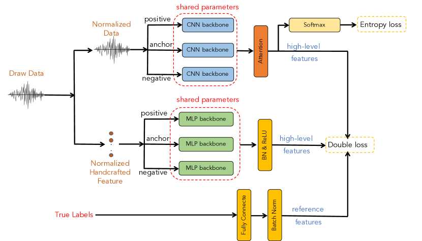
Figure 6: The robust deep learning based system with the proposed Double loss for MBFD task (Robust-MBFD).

To address the drawbacks of using Triplet losses, we propose a Double loss function in which the Triplet loss and Center loss are combined. In particular, we consider the embedding vectors denoted by C as consistent reference embedding vectors. These vectors are obtained from the true labels after passing through deep learning based layers (e.g., a fully connected layer followed by a Batch Normalization layer, as shown in the lower part of Fig. 6).

These reference embedding vectors help bring the anchor embedding vectors $\textbf{X}^{a}$ from the CNN-based backbone and the MLP-based backbone closer together, which is referred to as the Center loss. The Center loss aims to minimize the distance between anchor vectors and the reference vectors, represented as $d^{2}(\textbf{X}^{a},\textbf{C})$.

However, it’s important to note that the Center loss doesn’t affect other embedding vectors (e.g., positive or negative embedding vectors) apart from the anchor embedding vectors. To address this limitation, we integrate the Triplet loss into the Center loss. This combination ensures that all embedding vectors are positioned appropriately according to a specific rule: vectors of the same class need to be close, while those from different classes need to be distant. As a result, we formulate the distance computation among reference vectors, anchor vectors, positive vectors, and negative vectors for optimization by

$$H_{i}=\gamma(d^{2}(\mathbf{X}^{a}_{i},\mathbf{X}^{p}_{i})+d^{2}(\mathbf{X}^{a}_{i},\mathbf{C}_{i}))-d^{2}(\mathbf{X}^{a}_{i},\mathbf{X}^{n}_{i})+m$$ (6)

To optimize the performance, it is imperative to prioritize these components effectively, achieved through the parameter $\gamma$, which serves as a trade-off factor for balancing their contributions. After extensive experimentation, we found that setting $\gamma$ to 0.4 yields the best results. Additionally, we employ the symbol $m$ to signify a margin that enforces a clear separation between positive and negative pairs. Furthermore, we introduce $H_{i}$ as a standardization factor, which must be less than 0 to achieve the desired standardization. These elements collectively constitute our framework, ensuring the effectiveness and robustness of our approach.

TABLE X: Evaluating the Robust-MBFD system PU-C1 splitting method (training on artificial data and evaluating on real data), with different loss functions.

Method	Triplet loss	Center loss	Double loss
SVM	55.68	51.36	65.45
RF	52.61	51.70	63.29
KNN	42.27	49.20	61.81
Euclidean	42.50	49.43	72.72
Cosine	43.29	48.75	32.72
Ensemble	48.18	49.65	65.22

Given the distance formulations of $H^{S-SDML}_{i}$ and $H^{U-SDML}_{i}$ from two branches of the proposed Robust-MBFD model, our proposed Double losses of $\mathcal{L}_{double-S-SDML}$, $\mathcal{L}_{double-U-SDML}$ are described by Equation (7) and (8), respectively.

$$\mathcal{L}_{double-S-SDML}=\underset{\theta\in\mathbb{R}}{\text{argmin}}\sum_{i=1}^{n}\max(H^{S-SDML}_{i},0)$$ (7)

$$\mathcal{L}_{double-U-SDML}=\underset{\theta\in\mathbb{R}}{\text{argmin}}\sum_{i=1}^{n}\max(H^{U-SDML}_{i},0)$$ (8)

TABLE XI: Evaluating the proposed Robust-MBFD system on PU dataset with PU-C2 splitting method (training on real data and evaluating on real data)

	MAS	SS	RS	N	QT	PT
SVM	78.64	73.30	78.60	68.67	79.35	89.25
RF	78.32	69.50	73.50	74.40	88.36	88.75
KNN	68.25	76.60	78.90	78.40	78.70	84.08
Euclidean	73.36	74.40	77.63	77.61	88.60	90.91
Cosine	79.10	79.43	73.10	77.23	88.23	91.41

Combining these two Double losses, we achieve the loss:

$$\mathcal{L}_{2-Double}=\mathcal{L}_{double-S-SDML}+\lambda\mathcal{L}_{double-U-SDML}$$ (9)

The trade-off between the two Double loss functions is regulated by the parameter $\lambda$, which has been empirically set to 0.3 based on our experimental testing. Finally, we combine with the Cross-Entropy loss [56] which is applied for the first branch, then create the final loss to train the entire network. The ultimate loss function is expressed as follows:

$$\mathcal{L}=\mathcal{L}_{entropy}+\Lambda\mathcal{L}_{2-Double}$$ (10)

The value of $\Lambda$ is set to $0.01$ to mitigate perturbations in the gradient process, which will arise due to the computational complexity of $\mathcal{L}_{2-Double}$.

Given the Robust-MBFD system with the proposed novel Double loss, we achieved an accuracy score of 72.72%, as shown in Table X. This represents an improvement of approximately 20.00% compared to the individual deep learning base systems: SDLM, S-SDLM, or U-SDLM (all of which use the same Normalizer for normalization and SVM for back-end classification), as displayed in Table IX.

This result strongly indicates that the proposed Robust-MBFD system, incorporating the novel Double loss, is highly effective for the MBFD task. To demonstrate the superior performance of the Double loss, we conducted experiments comparing it to the Triplet loss and Center loss, while using the same network architecture depicted in Fig. 6. As Table X illustrates, the novel Double loss outperforms both the Triplet loss and the Center loss.

By combining the Robust-MBFD system with the novel Double loss, the Normalizer, and the back-end Euclidean measurement, we achieved the highest accuracy of 72.72% on the PU data with PU-C1 splitting.

IV-B Evaluating the proposed Robust-MBDF system on various datasets

As the proposed Robust-MBFD and the novel Double loss function help to achieve the best performance on the PU dataset with the splitting method of PU-C1, we further evaluate this system with the PU dataset using the PU-C2 splitting method and the other datasets of CWRU Bearing and MFPT Bearing using the splitting methods mentioned in Section 5.

TABLE XII: Evaluating the novel deep learning based system on CWRU datasets (Top-three scores are in bold)

	MAS	SS	RS	N	QT	PTF
CWRU-C1
SVM	38.71	69.38	68.42	83.27	84.05	69.55
RF	55.53	66.07	67.11	62.89	69.03	66.85
KNN	60.67	52.70	52.17	74.52	55.09	52.48
Euclidean	63.37	78.57	88.93	71.90	85.97	89.15
Cosine	62.15	78.91	88.89	69.72	85.27	87.71
CWRU-C2
SVM	42.76	46.32	63.54	62.30	70.06	65.23
RF	41.89	47.77	47.45	39.36	47.84	48.26
kNN	41.85	41.18	41.00	49.13	39.02	41.34
Euclidean	35.78	69.94	69.92	56.57	70.48	89.63
Cosine	34.23	68.54	70.02	57.63	71.56	90.01
CWRU-C3
SVM	25.30	45.23	29.56	55.57	56.68	29.65
Rf	33.89	38.17	38.43	28.33	38.28	38.65
kNN	36.96	35.19	35.60	43.54	29.18	35.34
Euclic	57.10	79.66	78.73	51.80	61.95	80.54
Cosine	58.63	81.78	77.21	52.23	60.89	81.57
CWRU-C4
SVM	77.03	88.39	82.41	83.88	87.15	90.32
RF	63.68	68.42	69.08	64.33	68.32	68.52
kNN	66.66	61.45	61.22	79.99	55.06	61.59
Euclidean	72.89	91.65	90.44	78.73	83.51	90.35
Cosine	73.68	90.32	89.66	77.21	84.69	89.65

TABLE XIII: Evaluating the robust deep learning based system on the MFPT dataset (Top-three scores are in bold)

	MAS	SS	RS	N	QT	PTF
SVM	99.11	99.90	99.86	89.22	98.78	97.51
RF	97.63	99.79	99.73	86.82	98.35	99.09
kNN	98.04	99.76	99.80	87.11	96.15	96.82
Euclic	98.70	99.66	99.56	89.30	98.32	99.12
Cosine	99.06	99.72	99.32	89.70	98.48	99.28

PU dataset with PU-C2 splitting: As the results on the PU dataset with the PU-C2 splitting method in Table XI show, the proposed robust deep learning based system achieves the best scores of 90.9% and 91.4% when using PowerTransformer normalization combined with Euclidean and Cosine distance measurements, respectively.

The results in Table XI also indicate that Euclidean and Cosine distance measurements outperform the machine learning based systems (i.e., SVM, RF, kNN) for classifying the concatenated high-level features.

The high performance on the PU dataset with the PC-C2 splitting method, compared to the low performance with the PC-C1 splitting method, can be explained by the fact that the PC-C2 splitting method uses only real data for both the training and evaluation processes. This also suggests potential applications in real-life scenarios when large amounts of authentic data are available.

CWRU dataset: The experimental results on the CWRU dataset with four splitting methods (e.g., CWRU-C1, CWRU-C2, CWRU-C3, CWRU-C4) are presented in Table XII. As shown in Table XII, almost all high accuracy scores are obtained from the Euclidean and Cosine distance measurements with PowerTransformer normalization. These results are similar to those observed on the PU dataset with the PU-C2 splitting method.

For all four splitting methods, the proposed robust deep learning based system consistently achieves accuracy rates of over 90.0%. This demonstrates the robustness of the proposed system on the CWRU dataset.

MFPT dataset: Looking at Table XIII, we achieved very high performance on the MFPT dataset with the best accuracy score of 99.9% (SVM for the back-end classification and SS for the normalization). Although high accuracy scores are observed in machine learning based classification methods such as SVM (99.9% with SS normalization and 99.8% with RS normalization) or RF (99.8% with SS normalization), the results from Euclidean and Cosine measurements are very competitive, with the best scores being 99.7% and 99.6% with SS normalization. We also observe that scores with SS normalization consistently achieve over 99.6% in this dataset.

V Conclusion

This paper presents a robust deep learning based system for Motor Bearing Fault Detection (Robust-MBFD). In the proposed Robust-MBFD system, three deep neural network architectures with different strategies of supervised, semi-supervised, and unsupervised learning, along with the proposed novel Double loss function, are combined to generate condensed and distinct high-level features that represent the raw vibration data. With these high-performing high-level features, Motor Bearing Faults can be detected using traditional machine learning based models (e.g., SVM, kNN, RF) or popular distance measurements (e.g., Euclidean and Cosine). Our extensive experiments on three benchmark datasets, namely PU Bearing, CWRU Bearing, and MFPT Bearing, with various data splitting methods, indicate that our proposed Robust-MBFD system is general and robust for the task of MBFD, making it highly suitable for real-life MBFD applications. Furthermore, our proposed Robust-MBFD system and our suggested splitting methods for these three datasets can serve as benchmark models and settings for the task of Motor Bearing Fault Detection (MBFD).

References

- [1] Austin H. Bonnett and Chuck Yung, “Increased efficiency versus increased reliability,” IEEE Industry Applications Magazine, vol. 14, no. 1, pp. 29–36, 2008.
- [2] Mounir Djeddi, Pierre Granjon, and Benoit Leprettre, “Bearing fault diagnosis in induction machine based on current analysis using high-resolution technique,” in 2007 IEEE International Symposium on Diagnostics for Electric Machines, Power Electronics and Drives, 2007, pp. 23–28.
- [3] Xiao Zhang, Boyang Zhao, and Yun Lin, “Machine learning based bearing fault diagnosis using the case western reserve university data: a review,” IEEE Access, vol. 9, pp. 155598–155608, 2021.
- [4] Henry O Omoregbee et al., Diagnosis and prognosis of rolling element bearings at low speeds and varying load conditions using higher order statistics and artificial intelligence, Ph.D. thesis, University of Pretoria, 2018.
- [5] Mao Wang, Niao-Qing Hu, Lei Hu, and Ming Gao, “Feature optimization for bearing fault diagnosis,” in 2013 International Conference on Quality, Reliability, Risk, Maintenance, and Safety Engineering (QR2MSE), 2013, pp. 1738–1741.
- [6] Hamed Helmi and Ahmad Forouzantabar, “Rolling bearing fault detection of electric motor using time domain and frequency domain features extraction and anfis,” IET Electric Power Applications, vol. 13, no. 5, pp. 662–669, 2019.
- [7] Tongle Xu, Junqing Ji, Xiaojia Kong, Fanghao Zou, and Wilson Wang, “Bearing fault diagnosis in the mixed domain based on crossover-mutation chaotic particle swarm,” Complexity, vol. 2021, 2021.
- [8] B. R. Nayana and P. Geethanjali, “Improved identification of various conditions of induction motor bearing faults,” IEEE Transactions on Instrumentation and Measurement, vol. 69, no. 5, pp. 1908–1919, 2020.
- [9] Sun Yue, Xu Aidong, Wang Kai, Han Xiaojia, Guo Haifeng, and Zhao Wei, “A novel bearing fault diagnosis method based on principal component analysis and bp neural network,” in 2019 14th IEEE International Conference on Electronic Measurement & Instruments (ICEMI), 2019, pp. 1125–1131.
- [10] Dongfang Zhao, Shulin Liu, Shouguo Cheng, Xin Sun, Lu Wang, Yuan Wei, and Hongli Zhang, “Dense multi-scale entropy and it’s application in mechanical fault diagnosis,” Measurement Science and Technology, vol. 31, no. 12, pp. 125008, 2020.
- [11] Keheng Zhu, Xigeng Song, and Dongxin Xue, “A roller bearing fault diagnosis method based on hierarchical entropy and support vector machine with particle swarm optimization algorithm,” Measurement, vol. 47, pp. 669–675, 2014.
- [12] Xin Li, Yu Yang, Haiyang Pan, Jian Cheng, and Junsheng Cheng, “A novel deep stacking least squares support vector machine for rolling bearing fault diagnosis,” Computers in Industry, vol. 110, pp. 36–47, 2019.
- [13] Wentao Mao, Liyun Wang, and Naiqin Feng, “A new fault diagnosis method of bearings based on structural feature selection,” Electronics, vol. 8, no. 12, pp. 1406, 2019.
- [14] Xin Wen, Guoliang Lu, Jie Liu, and Peng Yan, “Graph modeling of singular values for early fault detection and diagnosis of rolling element bearings,” Mechanical Systems and Signal Processing, vol. 145, pp. 106956, 2020.
- [15] Qingfeng Wang, Shuai Wang, Bingkun Wei, Wenwu Chen, and Yufei Zhang, “Weighted k-nn classification method of bearings fault diagnosis with multi-dimensional sensitive features,” IEEE Access, vol. 9, pp. 45428–45440, 2021.
- [16] Nannan Zhang, Lifeng Wu, Jing Yang, and Yong Guan, “Naive bayes bearing fault diagnosis based on enhanced independence of data,” Sensors, vol. 18, no. 2, pp. 463, 2018.
- [17] Fafa Chen, Mengteng Cheng, Baoping Tang, Baojia Chen, and Wenrong Xiao, “Pattern recognition of a sensitive feature set based on the orthogonal neighborhood preserving embedding and adaboost_svm algorithm for rolling bearing early fault diagnosis,” Measurement Science and Technology, vol. 31, no. 10, pp. 105007, 2020.
- [18] Christian Lessmeier, James Kuria Kimotho, Detmar Zimmer, and Walter Sextro, “Condition monitoring of bearing damage in electromechanical drive systems by using motor current signals of electric motors: A benchmark data set for data-driven classification,” in PHM Society European Conference, 2016, vol. 3.
- [19] Xin Huang, Guangrui Wen, Shuzhi Dong, Haoxuan Zhou, Zihao Lei, Zhifen Zhang, and Xuefeng Chen, “Memory residual regression autoencoder for bearing fault detection,” IEEE Transactions on Instrumentation and Measurement, vol. 70, pp. 1–12, 2021.
- [20] Jiedi Sun, Changhong Yan, and Jiangtao Wen, “Intelligent bearing fault diagnosis method combining compressed data acquisition and deep learning,” IEEE Transactions on Instrumentation and Measurement, vol. 67, no. 1, pp. 185–195, 2017.
- [21] Jianbo Yu, Xing Liu, and Lyujiangnan Ye, “Convolutional long short-term memory autoencoder-based feature learning for fault detection in industrial processes,” IEEE Transactions on Instrumentation and Measurement, vol. 70, pp. 1–15, 2020.
- [22] Linshan Jia, Tommy WS Chow, Yu Wang, and Yixuan Yuan, “Multiscale residual attention convolutional neural network for bearing fault diagnosis,” IEEE Transactions on Instrumentation and Measurement, vol. 71, pp. 1–13, 2022.
- [23] Junbin Chen, Ruyi Huang, Kun Zhao, Wei Wang, Longcan Liu, and Weihua Li, “Multiscale convolutional neural network with feature alignment for bearing fault diagnosis,” IEEE Transactions on Instrumentation and Measurement, vol. 70, pp. 1–10, 2021.
- [24] Gaowei Xu, Min Liu, Zhuofu Jiang, Weiming Shen, and Chenxi Huang, “Online fault diagnosis method based on transfer convolutional neural networks,” IEEE Transactions on Instrumentation and Measurement, vol. 69, no. 2, pp. 509–520, 2019.
- [25] Shuzhi Gao, Shuo Shi, and Yimin Zhang, “Rolling bearing compound fault diagnosis based on parameter optimization mckd and convolutional neural network,” IEEE Transactions on Instrumentation and Measurement, vol. 71, pp. 1–8, 2022.
- [26] Zhenxiang Li, Taisheng Zheng, Yang Wang, Zhi Cao, Zhiqi Guo, and Hongyong Fu, “A novel method for imbalanced fault diagnosis of rotating machinery based on generative adversarial networks,” IEEE transactions on instrumentation and measurement, vol. 70, pp. 1–17, 2020.
- [27] Pengfei Liang, Chao Deng, Jun Wu, Guoqiang Li, Zhixin Yang, and Yuanhang Wang, “Intelligent fault diagnosis via semisupervised generative adversarial nets and wavelet transform,” IEEE Transactions on Instrumentation and Measurement, vol. 69, no. 7, pp. 4659–4671, 2019.
- [28] Arnaz Malhi, Ruqiang Yan, and Robert X Gao, “Prognosis of defect propagation based on recurrent neural networks,” IEEE Transactions on Instrumentation and Measurement, vol. 60, no. 3, pp. 703–711, 2011.
- [29] Alex Shenfield and Martin Howarth, “A novel deep learning model for the detection and identification of rolling element-bearing faults,” Sensors, vol. 20, no. 18, pp. 5112, 2020.
- [30] Jinsong Yang, Jie Liu, Jingsong Xie, Changda Wang, and Tianqi Ding, “Conditional gan and 2-d cnn for bearing fault diagnosis with small samples,” IEEE Transactions on Instrumentation and Measurement, vol. 70, pp. 1–12, 2021.
- [31] Xinglong Pei, Xiaoyang Zheng, and Jinliang Wu, “Rotating machinery fault diagnosis through a transformer convolution network subjected to transfer learning,” IEEE Transactions on Instrumentation and Measurement, vol. 70, pp. 1–11, 2021.
- [32] Xu Wang, Changqing Shen, Min Xia, Dong Wang, Jun Zhu, and Zhongkui Zhu, “Multi-scale deep intra-class transfer learning for bearing fault diagnosis,” Reliability Engineering & System Safety, vol. 202, pp. 107050, 2020.
- [33] Ran Zhang, Hongyang Tao, Lifeng Wu, and Yong Guan, “Transfer learning with neural networks for bearing fault diagnosis in changing working conditions,” IEEE Access, vol. 5, pp. 14347–14357, 2017.
- [34] Olga Russakovsky, Jia Deng, Hao Su, Jonathan Krause, Sanjeev Satheesh, Sean Ma, Zhiheng Huang, Andrej Karpathy, Aditya Khosla, Michael Bernstein, Alexander C. Berg, and Li Fei-Fei, “ImageNet Large Scale Visual Recognition Challenge,” International Journal of Computer Vision (IJCV), , no. 3, pp. 211–252, 2015.
- [35] Christian Lessmeier, James Kuria Kimotho, Detmar Zimmer, and Walter Sextro, “Condition monitoring of bearing damage in electromechanical drive systems by using motor current signals of electric motors: A benchmark data set for data-driven classification,” in PHM Society European Conference, 2016, vol. 3.
- [36] Society for Machinery Failure Prevention Technology, “Bearing fault dataset,” https://www.mfpt.org/fault-data-sets/.
- [37] Case Western Reserve University, “Cwru dataset,” https://engineering.case.edu/bearingdatacenter/download-data-file.
- [38] James Kuria Kimotho and Walter Sextro, “An approach for feature extraction and selection from non-trending data for machinery prognosis,” in PHM Society European Conference, 2014, vol. 2.
- [39] Anssi Klapuri, Antti Eronen, and Jaakko Astola, “Analysis of the meter of acoustic musical signals,” Journal of the Acoustical Society of America, vol. 120, no. 1, pp. 391–399, 2007.
- [40] Ivan Miguel Pires, Faisal Hussain, Nuno M Garcia, Petre Lameski, and Eftim Zdravevski, “Homogeneous data normalization and deep learning: A case study in human activity classification,” Future Internet, vol. 12, no. 11, pp. 194, 2020.
- [41] Sergey I. and Christian S., “Batch normalization: Accelerating deep network training by reducing internal covariate shift,” in Proc. ICML, 2015, pp. 448–456.
- [42] V. Nair and G. E. Hinton, “Rectified linear units improve restricted boltzmann machines,” in ICML, 2010.
- [43] Florian Schroff, Dmitry Kalenichenko, and James Philbin, “Facenet: A unified embedding for face recognition and clustering,” in Proceedings of the IEEE conference on computer vision and pattern recognition, 2015, pp. 815–823.
- [44] Subhash Lele, “Euclidean distance matrix analysis (edma): estimation of mean form and mean form difference,” Mathematical Geology, vol. 25, pp. 573–602, 1993.
- [45] Case Western Reserve University, “Cwru data: Healthy data,” https://engineering.case.edu/bearingdatacenter/normal-baseline-data.
- [46] Case Western Reserve University, “Cwru data: 12k drive end bearing fault data,” https://engineering.case.edu/bearingdatacenter/12k-drive-end-bearing-fault-data.
- [47] Fabian Pedregosa, Gaël Varoquaux, Alexandre Gramfort, Vincent Michel, Bertrand Thirion, Olivier Grisel, Mathieu Blondel, Peter Prettenhofer, Ron Weiss, Vincent Dubourg, Jake Vanderplas, Alexandre Passos, David Cournapeau, Matthieu Brucher, Matthieu Perrot, and Édouard Duchesnay, “Scikit-learn: Machine learning in python,” Journal of Machine Learning Research, vol. 12, no. 85, pp. 2825–2830, 2011.
- [48] P. K. Diederik and B. Jimmy, “Adam: A method for stochastic optimization,” CoRR, vol. abs/1412.6980, 2015.
- [49] Ekaba Bisong and Ekaba Bisong, “Introduction to scikit-learn,” Building Machine Learning and Deep Learning Models on Google Cloud Platform: A Comprehensive Guide for Beginners, pp. 215–229, 2019.
- [50] Shoichi Ichimura and Qiangfu Zhao, “Route-based ship classification,” in 2019 IEEE 10th International Conference on Awareness Science and Technology (iCAST). IEEE, 2019, pp. 1–6.
- [51] Subhatav Dhali, Monalisha Pati, Soumi Ghosh, and Chandan Banerjee, “An efficient predictive analysis model of customer purchase behavior using random forest and xgboost algorithm,” in 2020 IEEE 1st International Conference for Convergence in Engineering (ICCE). IEEE, 2020, pp. 416–421.
- [52] Eduardo Gonçalves Freitas, João P Matos-Carvalho, and Rui Manuel Tavares, “Ripening assessment classification using artificial intelligence algorithms with electrochemical impedance spectroscopy data,” in 2023 7th International Young Engineers Forum (YEF-ECE). IEEE, 2023, pp. 20–25.
- [53] Harshith Reddy Takkala, Vinay Khanduri, Aniket Singh, Sai Nikhil Somepalli, Rakesh Maddineni, and Sankha Patra, “Kyphosis disease prediction with help of randomizedsearchcv and adaboosting,” in 2022 13th International Conference on Computing Communication and Networking Technologies (ICCCNT). IEEE, 2022, pp. 1–5.
- [54] Ricardo Manuel Arias Velásquez, “Support vector machine and tree models for oil and kraft degradation in power transformers,” Engineering Failure Analysis, vol. 127, pp. 105488, 2021.
- [55] Fabian Pedregosa, Gaël Varoquaux, Alexandre Gramfort, Vincent Michel, Bertrand Thirion, Olivier Grisel, Mathieu Blondel, Peter Prettenhofer, Ron Weiss, Vincent Dubourg, et al., “Scikit-learn: Machine learning in python,” the Journal of machine Learning research, vol. 12, pp. 2825–2830, 2011.
- [56] Yaoshiang Ho and Samuel Wookey, “The real-world-weight cross-entropy loss function: Modeling the costs of mislabeling,” IEEE access, vol. 8, pp. 4806–4813, 2019.