Modeling lower-truncated and right-censored insurance claims with an extension of the MBBEFD class

Abstract

In general insurance, claims are often lower-truncated and right-censored because insurance contracts may involve deductibles and maximal covers. Most classical statistical models are not (directly) suited to model lower-truncated and right-censored claims. A surprisingly flexible family of distributions that can cope with lower-truncated and right-censored claims is the class of MBBEFD distributions that originally has been introduced by Bernegger (1997) for reinsurance pricing, but which has not gained much attention outside the reinsurance literature. We derive properties of the class of MBBEFD distributions, and we extend it to a bigger family of distribution functions suitable for modeling lower-truncated and right-censored claims. Interestingly, in general insurance, we mainly rely on unimodal skewed densities, whereas the reinsurance literature typically proposes monotonically decreasing densities within the MBBEFD class.

Keywords. General insurance claims, lower-truncation, right-censoring, MBBEFD distribution, unimodal density, skewed density, normalized loss, exposure curve, Swiss Re exposure curve, Lloyd’s exposure curve.

1 Introduction

Insurance contracts in general insurance often involve deductibles $d>0$ and maximal covers $M>0$. Deductibles are introduced to reduce the number of small claims which mainly cause administrative expenses but which are not essential in risk mitigation. Maximal covers are introduced to control the maximal loss of an insurer. A maximal cover may, e.g., refer to the property value insured (after subtracting the deductible), or to the maximal insurance coverage warranted to a liability claim. Denote by $Y^{\dagger}$ the total financial loss. The insurance claim $Y$ after subtracting the deductible $d>0$ and with a maximal cover of size $M>0$ is given by

$$Y=\min\left\{(Y^{\dagger}-d)_{+},\,M\right\}.$$ (1.1)

We say, this financial loss is lower-truncated at $d>0$ and right-censored at $M>0$ (after subtracting the deductible). Statistical modeling of lower-truncated and right-censored claims is a notoriously difficult problem because most statistical models have an unbounded support, e.g., the supports of the gamma and the log-normal distributions are the entire positive real line ${\mathbb{R}}_{+}$. In most cases, this implies that fitting a statistical model to lower-truncated and right-censored data is not a problem that is easily analytically tractable. We give an example. We start from a classical statistical model such as the gamma distribution for the total financial loss $Y^{\dagger}\sim F_{\Gamma}$, where $F_{\Gamma}$ denotes the gamma distribution with corresponding gamma density $f_{\Gamma}$ on ${\mathbb{R}}_{+}$. Lower-truncation and right-censoring introduces two difficulties which are illustrated in Figure 1. First, the lower-truncation $(Y^{\dagger}-d)_{+}$ of the total financial loss $Y^{\dagger}$ implies, in general, that the density of the lower-truncated claim is positive in 0, see Figure 1. In the above mentioned gamma case, this means that the lower-truncation with $d>0$ leads to a new density given by

$$y\geq 0~{}\mapsto~{}\frac{f_{\Gamma}(d+y)}{\int_{d}^{\infty}f_{\Gamma}(z)\,dz}=\frac{f_{\Gamma}(d+y)}{1-F_{\Gamma}(d)}~{}>~{}0.$$

Second, right-censoring at $M>0$ of this lower-truncated claim $(Y^{\dagger}-d)_{+}$ leads to a point mass in $M$, resulting in the density $f$ of the lower-truncated and right-censored claim $Y$

$$y\geq 0~{}\mapsto~{}f(y)=\frac{f_{\Gamma}(d+y)}{1-F_{\Gamma}(d)}\,\mathds{1}_{\{y<M\}}+\frac{1-F_{\Gamma}(d+M)}{{1-F_{\Gamma}(d)}}\,\mathds{1}_{\{y=M\}},$$ (1.2)

where (1.2) is a density w.r.t. the $\sigma$-finite measure being the Lebesgue measure on $(0,M)$ and having a point mass in $M$; this point mass is not illustrated in Figure 1, but only the absolutely continuous part on $(0,M)$; the point mass in $M$ equals one minus the volume of the blue area in Figure 1.

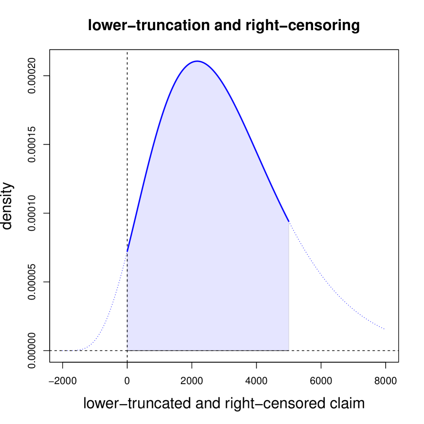
Figure 1: Lower-truncated and right-censored claim with $d=2000$ and $M=5000$.

More generally, for maximum likelihood estimation (MLE) based on lower-truncated and right-censored claims $Y\in(0,M]$, ${\mathbb{P}}$-a.s., we consider the log-likelihood function of an unknown parameter $\theta$ given by

$$\theta~{}\mapsto~{}\ell_{Y}(\theta)=\log\left(f_{\theta}(Y)\right)\mathds{1}_{\{Y<M\}}+\log\left(1-F_{\theta}(M_{-})\right)\mathds{1}_{\{Y=M\}},$$ (1.3)

assuming that the response variable $Y$ is absolutely continuous on $(0,M)$ with density $f_{\theta}(y)$, having a point mass $1-F_{\theta}(M_{-})=1-\lim_{y\uparrow M}F_{\theta}(y)$ in $M$, and with (unknown) model parameter $\theta$. Fitting such a model with MLE can be difficult because we need an analytically tractable form for both the density $f_{\theta}(\cdot)$ and its distribution function $F_{\theta}(\cdot)$, see (1.3). This is not the case, e.g., in the lower-truncated and right-censored gamma model given in (1.2). Therefore, in such cases, one either needs to rely on numerical integration of the density (which can be computationally demanding) or one uses a version of the Expectation-Maximization (EM) algorithm by interpreting the lower-truncation and right-censoring as a missing information problem; we refer to Verbelen et al. [16], Fung et al. [5] and Sections 6.4.2 and 6.4.3 in Wüthrich–Merz [17]. However, also this EM algorithm approach has its drawbacks as it requires tractability of conditional tail expectations and reasonable dispersion estimates in multi-dimensional parameter settings. These two side constraints lead to further restrictions on the class of solvable models, e.g., these problems can only be solved for a very small number of models within the class of Tweedie’s models [15], namely, for the Tweedie’s models stated in Theorem 3 of Blæsild–Jensen [3]; we also refer to Landsman–Valdez [6]. In a series of papers, Poudyal [9, 10] and Poudyal–Brazauskas [11] consider trimmed and/or winsorized method of moments estimators for truncated and/or censored data; in statistics, truncation is also called trimming and censoring winsorizing. In these papers, trimming and winsorizing is also shown to be a useful method of robustifying moment estimation under extreme claims.

We take a different approach in this paper to solve the fitting problem of lower-truncated and right-censored data. In reinsurance, often so-called MBBEFD exposure curves are used for exposure rating. Those exposure curves have been introduced by Bernegger [2], and the acronym MBBEFD indicates that this class includes the Maxwell–Boltzmann (MB), the Bose–Einstein (BE) and the Fermi–Dirac (FD) distributions; these are well known distributions in statistical mechanics. These MBBEFD exposure curves are based on the assumption that there is a maximal cover $M$, and they directly describe right-censored claims up to this maximal cover. Differentiating twice these MBBEFD exposure curves provides us with densities being absolutely continuous on the interval $(0,M)$ and having a point mass in $M$; we refer to formula (3.7) in Bernegger [2].

The goal of this paper is first to study the properties of these MBBEFD densities and to extend it to a bigger class of models that will be called the Bernegger class. Our contribution is to show that the Bernegger class is rather rich including monotonically decreasing densities, unimodal densities and monotonically increasing densities, and our extension provides new families of lower-truncated and right-censored random variables that allow for skewness in the absolutely continuous part of the distribution. This is of particular interest because unimodal skewed densities are suited for modeling lower-truncated and right-censored claims in general insurance since their empirical density roughly looks like the one given in Figure 1. In particular, one can recognize the distribution of right-censored exponential random variables as a special case of the Bernegger class.

Surprisingly, the class of MBBEFD densities of Bernegger [2] has only entered the reinsurance literature; see, e.g., Parodi–Watson [8], Abramson [1], Riegel [13], Chapter 21 of Parodi [7], and the R [12] package mbbefd of Dutang et al. [4, 14]. Popular examples in reinsurance pricing are the so-called Swiss Re and Lloyd’s exposure curves that are special cases of MBBEFD exposure curves; see Bernegger [2]. However, in this reinsurance pricing literature, one mainly focuses on exposure curves and not on the resulting densities nor on their properties. We show that the most popular choices from reinsurance lead to monotonically decreasing densities, whereas we are mainly interested into the unimodal case, as this is the common situation in general insurance pricing, e.g., in private insurance lines.

Organization. This manuscript is organized as follows. In the next section, we state the necessary properties that any exposure curve has to fulfill in order to describe distribution functions allowing to model lower-truncated and right-censored claims. In Section 3, we start from the MBBEFD class of distributions of Bernegger [2] by stating some of its properties, and then we extend it to a richer family of distributions, the Bernegger class. In Section 4, we introduce a subclass of the Bernegger class that incorporates the MBBEFD class of distributions, whereas in Section 5, we treat another subclass of distributions that includes the exponential distribution. In Section 6, we use a real dataset of lower-truncated and right-censored claims in order to compare the performance of the MBBEFD class of distributions to four other classes of distributions when trying to fit those models using maximum likelihood estimation (MLE). Finally, the last section concludes this work. All mathematical proofs are provided in the appendix.

2 Exposure curves and their resulting densities

2.1 From Exposure curves to distributions

In reinsurance claims modeling, one often works with exposure curves instead of distribution functions. Assume we have a positively supported response variable $Y\sim F_{Y}$, and assume that the maximal possible loss (MPL) is given by $M>0$, i.e., $0<Y\leq M$, ${\mathbb{P}}$-a.s. We define the normalized loss $Z=Y/M$. Denote the distribution function of the normalized loss $Z$ by $F_{Z}$, being supported in $(0,1]$. The exposure curve of a normalized loss $Z\sim F_{Z}$ is given by

$$z~{}\mapsto~{}G(z)=\frac{\int_{0}^{z}1-F_{Z}(s)\,ds}{\int_{0}^{1}1-F_{Z}(s)\,ds}=\frac{\int_{0}^{z}1-F_{Z}(s)\,ds}{{\mathbb{E}}[Z]},$$

for $z\in[0,1]$; see Bernegger [2]. This exposure curve $G:[0,1]\to[0,1]$ is non-decreasing, concave, and satisfies the property $G^{\prime}(0)>0$, as well as the normalization $G(0)=0$ and $G(1)=1$; for examples see Figure 2 (lhs), below. In the last integral, a change of variable $s\in[0,1]\mapsto t=sM\in[0,M]$ gives us

$$G(z)=\frac{\int_{0}^{zM}1-F_{Z}(t/M)\,dt}{M{\mathbb{E}}[Z]}=\frac{\int_{0}^{zM}1-F_{Y}(t)\,dt}{{\mathbb{E}}[Y]}=G_{Y}(zM),$$

the latter being the exposure curve of $Y$ on $[0,M]$. Thus, we can equally work with the responses $Y$ and $Z$, but the normalized losses $Z$ will have the advantage that they live on a common unit interval $[0,1]$. Now, let us take the opposite view and characterize the distribution function of a random variable $Z\sim F_{Z}$ obtained from a function $G:[0,1]\rightarrow\mathbb{R}$ satisfying the same properties of an exposure curve. Under the assumptions of the next theorem, this distribution $F_{Z}$ leads to an absolutely continuous density on $[0,1)$ and a point mass at 1.

Theorem 2.1.

Let $G:[0,1]\rightarrow\mathbb{R}$ be a non-decreasing, concave, and twice continuously differentiable function with $G(0)=0,\,G(1)=1,\,G^{\prime}(0)>0$. The function $F_{Z}:[0,1]\rightarrow\mathbb{R}$ defined by

$$F_{Z}(z)=\left(1-\frac{G^{\prime}(z)}{G^{\prime}(0)}\right)\mathds{1}_{\{z<1\}}+\mathds{1}_{\{z=1\}}$$ (2.1)

is a distribution function on $[0,1]$. Furthermore, this distribution has as density

$$f_{Z}(z)=-\frac{G^{\prime\prime}(z)}{G^{\prime}(0)},$$ (2.2)

for $z\in[0,1)$, and a point mass at 1 given by

$$p=\frac{G^{\prime}(1)}{G^{\prime}(0)}.$$ (2.3)

Finally, the mean of $Z\sim F_{Z}$ is equal to ${\mathbb{E}}[Z]=1/G^{\prime}(0)$.

The proofs of all statements are given in the appendix. Due to this last result, functions $G$ satisfying the assumptions of Theorem 2.1 will be called exposure curves.

Definition 2.2.

An exposure curve is a function $G:[0,1]\rightarrow\mathbb{R}$, which is non-decreasing, concave, and twice continuously differentiable with $G(0)=0,\,G(1)=1,\,G^{\prime}(0)>0$.

As seen previously, if we start from any such function $G$, we can derive a distribution whose density is absolutely continuous and of closed form on $[0,1)$, with a point mass in 1 and a mean that are of closed form too, i.e., we have a class of models that has a full tractable mean, density and point mass, which is suitable to model right-censored claims, and if $G^{\prime\prime}(0)<0$, we can also consider lower-truncation, see (2.2). It turns out that a linear combination of exposure curves allows us to define a mixture of their respective associated distribution functions as the next result shows.

Lemma 2.3.

Let $(\alpha_{i})_{i=1}^{n}$ be non-negative weights adding up to 1 and let $(G_{i})_{i=1}^{n}$ be exposure curves leading to distributions functions $(F_{i})_{i=1}^{n}$, densities $(f_{i})_{i=1}^{n}$, and point masses in 1 equal to $(p_{i})_{i=1}^{n}$ as in Theorem 2.1. The convex combination

$$G(z)=\sum_{i=1}^{n}\alpha_{i}G_{i}(z),$$ (2.4)

for $z\in[0,1]$, is again an exposure curve, allowing to define the distribution function of a random variable $Z\sim F_{Z}$ given by

$$F_{Z}(z)=\sum_{i=1}^{n}w_{i}F_{i}(z),$$

for $z\in[0,1]$, and where $w_{i}=\alpha_{i}G_{i}^{\prime}(0)/\sum_{j=1}^{n}\alpha_{j}G_{j}^{\prime}(0)$ are non-negative weights summing up to 1. In particular, the density of $Z$ on $[0,1)$ is given by

$$f_{Z}(z)=\sum_{i=1}^{n}w_{i}f_{i}(z),$$

and the point mass in 1 is equal to

$$p=\sum_{i=1}^{n}w_{i}p_{i}.$$

Finally, the mean of $Z\sim F_{Z}$ is given by

$${\mathbb{E}}[Z]=\sum_{i=1}^{n}w_{i}\,\frac{1}{G_{i}^{\prime}(0)}.$$

2.2 Flexibility of the point mass in the right-censoring point

The point mass $p$ in 1 is automatically determined by formula (2.3). Often, one may require more modeling flexibility in the choice of this point mass, while still retaining the tractability of the density and the mean as it was shown in Theorem 2.1. A simple way to do so connects to so-called one-inflated distributions; we refer to Dutang et al. [4]. In the case of Theorem 2.1, this can easily be achieved. The next corollary shows, how we can obtain them by looking at the conditional density of the random variable $Z_{0}\stackrel{{\scriptstyle\rm(d)}}{{=}}Z|_{\{Z<1\}}$.

Corollary 2.4.

Let $G:[0,1]\rightarrow\mathbb{R}$ be an exposure curve, we receive an absolutely continuous density on $[0,1)$ given by

$$\begin{split}f_{0}(z)=-\frac{1}{1-p}\frac{G^{\prime\prime}(z)}{G^{\prime}(0)}=\frac{G^{\prime\prime}(z)}{G^{\prime}(1)-G^{\prime}(0)}~{}\geq~{}0,\end{split}$$

which integrates to 1. This density provides the mean for the random variable $Z_{0}\sim f_{0}$

$${\mathbb{E}}[Z_{0}]=\frac{1}{1-p}({\mathbb{E}}[Z]-p)=\frac{1-G^{\prime}(1)}{G^{\prime}(0)-G^{\prime}(1)}.$$

We can now add a point mass $q\in(0,1)$ at 1 to this density. This adds one more parameter to the model, giving us a mixture distribution between an absolutely continuous part $f_{0}$ on $[0,1)$ and a point mass in 1. We have the following corollary.

Corollary 2.5.

Let $G:[0,1]\rightarrow\mathbb{R}$ be an exposure curve, the random variable $Z$ that has an absolutely continuous density on $[0,1)$ given by

$$f_{q}(z)=\left(1-q\right)\frac{G^{\prime\prime}(z)}{G^{\prime}(1)-G^{\prime}(0)}~{}\geq~{}0,$$

with fixed point mass $q\in(0,1)$ in 1 has expected value

$${\mathbb{E}}[Z]=\left(1-q\right)\frac{1-G^{\prime}(1)}{G^{\prime}(0)-G^{\prime}(1)}+q.$$

Note that the transformation achieved in Corollary 2.5 can also be obtained using Lemma 2.3. Indeed, let us consider the function

$$\tilde{G}(z)=w\,G(z)+(1-w)z,$$

for $z\in[0,1]$, $w\in[0,1]$, and where $G$ is an exposure curve. Then, the function $\tilde{G}$ is an exposure curve. Using Theorem 2.1, if we denote by $F$ the distribution function obtained from the exposure curve $G$, by $f$ the absolutely continuous density on $[0,1)$ and by $p$ the point mass in 1, we can characterize the distribution function $\tilde{F}$, the absolutely continuous density on $[0,1)$ $\tilde{f}$, and the point mass $\tilde{p}$ obtained from the exposure curve $\tilde{G}$ using

$$\tilde{F}(z)=wF(z)+(1-w)\mathds{1}_{\{z=1\}},$$

for $z\in[0,1]$,

$$\quad\tilde{f}(z)=wf(z)=-w\frac{G^{\prime\prime}(z)}{G^{\prime}(0)},$$

for $z\in[0,1)$, and

$$\tilde{p}=wp+(1-w).$$

In what follows, the goal will be to introduce examples of exposure curves that are useful to model lower-truncated and right-censored losses. Before that, we start by studying the explicit family of exposure curves introduced by Bernegger [2].

3 The Bernegger class of distributions

3.1 The class of MBBEFD exposure curves and densities

The MBBEFD class of Bernegger [2] selects an explicit family of exposure curves. This family is parametrized through two parameters $g\geq 1$ and $b\geq 0$, and is given as follows for $z\in[0,1]$

$$G_{b,g}(z)=\left\{\begin{array}[]{ll}z&\text{ for $g=1$ or $b=0$,}\\ \frac{\log(1+(g-1)z)}{\log(g)}&\text{ for $g>1$ and $b=1$,}\\ \frac{1-b^{z}}{1-b}&\text{ for $g>1$ and $bg=1$,}\\ \frac{\log\left(\frac{(g-1)b+(1-bg)b^{z})}{(1-b)}\right)}{\log(bg)}&\text{ for $g>1$, $b>0$, $b\neq 1$ and $bg\neq 1$.}\end{array}\right.$$ (3.1)

The three cases $bg=1$, $bg>1$ and $bg<1$ give the MB (Maxwell-Boltzmann), the BE (Bose-Einstein) and the FD (Fermi-Dirac) distributions, respectively. Using (2.1), we can calculate the distributions for $z\in[0,1)$, see (3.6) in Bernegger [2],

$$F_{b,g}(z)=\left\{\begin{array}[]{ll}0&\text{ for $g=1$ or $b=0$,}\\ 1-\left(1+(g-1)z\right)^{-1}&\text{ for $g>1$ and $b=1$,}\\ 1-b^{z}&\text{ for $g>1$ and $bg=1$,}\\ 1-\frac{1-b}{(g-1)b^{1-z}+(1-bg)}&\text{ for $g>1$, $b>0$, $b\neq 1$ and $bg\neq 1$.}\end{array}\right.$$ (3.2)

We observe that the first case is not of interest because it gives a point mass of 1 to $z=1$. For this reason, we skip this case in the sequel. On $z<1$, we can calculate the second derivatives of these exposure curves $G_{b,g}$. This gives us the densities for $z\in[0,1)$, see (3.7) in Bernegger [2],

$$f_{b,g}(z)=\left\{\begin{array}[]{ll}(g-1)\left(1+(g-1)z\right)^{-2}&\text{ for $g>1$ and $b=1$,}\\ -\log(b)b^{z}&\text{ for $g>1$ and $bg=1$,}\\ \frac{(g-1)(b-1)\log(b)b^{1-z}}{\left((g-1)b^{1-z}+(1-bg)\right)^{2}}&\text{ for $g>1$, $b>0$, $b\neq 1$ and $bg\neq 1$,}\end{array}\right.$$ (3.3)

and we have a point mass in $z=1$ given by

$$p=\frac{1}{g}~{}\in~{}(0,1).$$ (3.4)

Thus, we have an absolutely continuous distribution on $[0,1)$, with a point mass $p=1/g$ in 1, and, e.g., in the last case of (3.3), we have a strictly positive density in 0

$$f_{b,g}(0)=\frac{(g-1)\log(b)b}{b-1}~{}>~{}0.$$

Such a density may therefore come from a lower-truncated claim. Finally, the mean is given by

$${\mathbb{E}}_{b,g}[Z]=\left\{\begin{array}[]{ll}\frac{\log(g)}{g-1}&\text{ for $g>1$ and $b=1$,}\\ \frac{b-1}{\log(b)}&\text{ for $g>1$ and $bg=1$,}\\ \frac{b-1}{\log(b)}\frac{\log(bg)}{bg-1}&\text{ for $g>1$, $b>0$, $b\neq 1$ and $bg\neq 1$.}\end{array}\right.$$ (3.5)

We give an example of such an exposure curve that is typically used for exposure rating in reinsurance.

Example 3.1 (Swiss Re and Lloyd’s exposure curves).

Bernegger [2] provides an explicit parametrization for the MBBEFD class which can be used for reinsurance exposure rating in case of scarce data. Namely, both parameters $b$ and $g$ are parametrized as a function of a single parameter $c>0$ as follows

$$b=b(c)=\exp\{3.1-0.15(1+c)c\}\qquad\text{ and }\qquad g=g(c)=\exp\{(0.78+0.12c)c\}.$$ (3.6)

For $c=1.5,2,3,4$, one obtains the Swiss Re exposure curves, and for $c=5$, the Lloyd’s exposure curve, these are illustrated in Figure 2 (lhs). The right-hand side of this figure shows the resulting densities $f_{b(c),g(c)}(\cdot)$, and we remark that all of the resulting MBBEFD densities are monotonically decreasing on $(0,1)$. $\blacksquare$

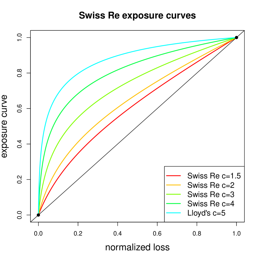
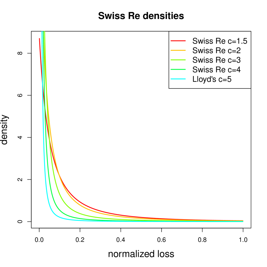
Figure 2: Swiss Re and Lloyd’s exposure curves (lhs) and the resulting densities (rhs).

3.2 Properties of the MBBEFD class

Example 3.1 has shown that the exposure curves (3.6) proposed by Bernegger [2] for reinsurance exposure rating lead to monotonically decreasing densities $f_{b,g}$, see Figure 2 (rhs). For general insurance pricing, we are rather interested into unimodal densities similar to Figure 1, because this more commonly reflects the properties of general insurance claims data.

Proposition 3.2.

The density $f_{b,g}$ for $g>1$ and $b>0$ given in (3.3) has the following properties:

• Case $bg<1$. The density $f_{b,g}$ is

  • monotonically decreasing on $[0,1)$ for $(1-bg)/(g-1)\leq b$;

  • unimodal on $[0,1)$ for $b<(1-bg)/(g-1)<1$, with a maximum in

    $$z^{*}=1-\frac{\log\left((1-bg)/(g-1)\right)}{\log(b)}~{}\in~{}(0,1);$$ (3.7)

  • monotonically increasing on $[0,1)$ for $(1-bg)/(g-1)\geq 1$.

• Case $bg\geq 1$. The density $f_{b,g}$ is monotonically decreasing on $[0,1)$.

This proposition shows that in practical applications in general insurance, the FD distributions (with $bg<1$) are the most interesting ones, as they can be unimodal, or either monotonically decreasing or increasing. This excludes the exposure curves of Example 3.1, as these Swiss Re and Lloyd’s exposure curves provide us with $bg>1$. Next, we show that the MBBEFD distribution $F_{b,g}$ for $bg<1$ can be derived from the logistic function (distribution)

$$\psi(t)=\frac{e^{t}}{e^{t}+1}~{}\in~{}(0,1),$$

for $t\in{\mathbb{R}}$. The logistic function has first derivative (logistic density)

$$\psi^{\prime}(t)=\frac{e^{t}}{(e^{t}+1)^{2}}=\psi(t)\left(1-\psi(t)\right).$$

This derivative is symmetric around zero. We have the following result.

Proposition 3.3.

Let $b>0$ and $g>1$. For $bg<1$, the MBBEFD density has the functional form, for $z\in[0,1)$,

$$f_{b,g}(z)=(a+1)\log(1/b)\,\psi^{\prime}\left(z\log(1/b)+\log(a)\right),$$

where we set

$$a=\frac{b(g-1)}{1-bg}\qquad\text{ and }\qquad g=\frac{a+b}{(a+1)b},$$ (3.8)

respectively. If $b<(1-bg)/(g-1)<1$, i.e. $b<a<1$, this MBBEFD density is bell shaped around $z^{*}$ given in (3.7).

For further terminology, we call unimodal symmetric densities, bell shaped densities. Of course, this includes for example the Gaussian density but also the logistic density. We conclude that for $bg<1$, the MBBEFD density is the logistic density $\psi^{\prime}$ on the interval

$$\left[\log(a),\,\log(a/b)\right),$$

scaled by a constant factor $(1+a)\log(1/b)>0$. It is symmetric around the mode $z^{*}$, and it decays slower than the Gaussian density. This now shows why the MBBEFD densities are not sufficient for general insurance claims modeling, because general insurance claims are typically positively skewed, which cannot be captured by the logistic density.

3.3 Extension of Bernegger’s idea using non-bell shaped densities

We extend the class of bell-shaped MBBEFD densities to a more general class of exposure curves, which allows, in particular, for skewness in their corresponding densities. We call this extended family the Bernegger class. In Section 2.1, we have started from a generic exposure curve $G:[0,1]\to[0,1]$ which is a non-decreasing, concave and twice continuously differentiable function with the normalization $G(0)=0,\,G(1)=1$ and with $G^{\prime}(0)>0$. The MBBEFD exposure curve (3.1) can be reparametrized. Indeed, by using (3.8), we obtain for $z\in[0,1]$

$$G_{b,a}(z)=\frac{\log(a+b^{z})-\log(a+1)}{\log(a+b)-\log(a+1)},$$ (3.9)

for $b\geq 0$ and $a>-\min(1,b)$; we refer to Section 3.1 of Bernegger [2]. This structure can be used to design exposure curve forms that do not have the bell-shape property of Proposition 3.3. The function $a+b^{z}=a+\exp\{-z\log(1/b)\}$ is strictly decreasing and convex for $b\in(0,1)$. We modify the modeling set-up (3.9) as follows. Choose a function $B:[0,1]\rightarrow{\mathbb{R}}$ that satisfies

$$B(z)=h(b(z)),$$ (3.10)

for some functions $h$ and $b$, in order to define an exposure curve (under further assumptions on $h$ and $b$)

$$z\mapsto G(z)=\frac{B(z)-B(0)}{B(1)-B(0)},$$ (3.11)

which ensures that the normalization property $G(0)=0$ and $G(1)=1$ is satisfied. The function $h$ will be denoted as the link function, whereas the function $b$ will be named the inner function, and we notice that Bernegger’s original choice was $b(z)=a+b^{z}$ for $b\in(0,1)$ and $h(x)=\log(x)$, meaning that he used a logarithmic linked exposure curve. We will first explore some examples using the same link function and then introduce the exponentially linked exposure curves, which use the link function $h(x)=\exp(x)$ and seem to be more suitable in modeling general insurance claims. We call the class of distributions induced by exposure curves of the form (3.11) the Bernegger class.

4 Logarithmic linked exposure family

We start by considering logarithmic linked examples of the Bernegger class, which are obtained by choosing $h(x)=\log(x)$ in (3.10).

Proposition 4.1.

Choose a function $b:[0,1]\to(0,\infty)$ with $b(0)\neq b(1)$ that is twice continuously differentiable and define for $z\in[0,1]$ the function

$$G(z)=\frac{\log(b(z))-\log(b(0))}{\log(b(1))-\log(b(0))}.$$ (4.1)

The function $G$ is an exposure curve if and only if one of the following holds:

$$b^{\prime}(0)>0,\,b^{\prime}(z)\geq 0\textrm{ and }b^{\prime\prime}(z)b(z)-b^{\prime}(z)^{2}\leq 0\textrm{ for all }z\in[0,1],$$ (4.2)

or

$$b^{\prime}(0)<0,\,b^{\prime}(z)\leq 0\textrm{ and }b^{\prime\prime}(z)b(z)-b^{\prime}(z)^{2}\geq 0\textrm{ for all }z\in[0,1].$$ (4.3)

Using Theorem 2.1, one can then derive the distribution function of a random variable leading to an absolutely continuous density on $[0,1)$ and a point mass in 1.

Corollary 4.2.

Assume that a twice continuously differentiable function $b:[0,1]\to(0,\infty)$ with $b(0)~{}\neq~{}b(1)$ fulfills condition (4.2) or (4.3). The exposure curve $G$ defined in (4.1) provides the distribution of a random variable $Z\sim F_{Z}$

$$F_{Z}(z)=\left(1-\frac{b^{\prime}(z)}{b^{\prime}(0)}\frac{b(0)}{b(z)}\right)\mathds{1}_{\{z<1\}}+\mathds{1}_{\{z=1\}},$$ (4.4)

for $z\in[0,1]$, with density for $z\in[0,1)$

$$f_{Z}(z)=\frac{b(0)}{-b^{\prime}(0)}\frac{b^{\prime\prime}(z)b(z)-b^{\prime}(z)^{2}}{b(z)^{2}},$$

and with point mass in $z=1$ equal to

$$p=\frac{b^{\prime}(1)}{b^{\prime}(0)}\frac{b(0)}{b(1)}.$$

Moreover, the mean of $Z\sim F_{Z}$ is equal to

$${\mathbb{E}}[Z]=\frac{b(0)}{-b^{\prime}(0)}\,\log\left(\frac{b(0)}{b(1)}\right).$$

For general insurance pricing, we are interested into unimodal densities and one is thus interested in the first derivative of $f_{Z}$ in order to characterize the maximum of the density

$$f^{\prime}_{Z}(z)=\frac{b(0)}{-b^{\prime}(0)}\frac{b^{\prime\prime\prime}(z)b(z)^{2}-3b^{\prime\prime}(z)b^{\prime}(z)b(z)+2b^{\prime}(z)^{3}}{b(z)^{3}}.$$

Note that this derivative only exists if the third derivative of $b$ exists.

5 Exponentially linked exposure family

Next we introduce the exponentially linked exposure family by setting $h(x)=\exp(x)$ in (3.10).

Proposition 5.1.

Choose a function $b:[0,1]\to{\mathbb{R}}$ with $b(0)\neq b(1)$ that is twice continuously differentiable and define for $z\in[0,1]$ the function

$$G(z)=\frac{e^{b(z)}-e^{b(0)}}{e^{b(1)}-e^{b(0)}}.$$ (5.1)

The function $G$ is an exposure curve if and only if one of the following holds:

$$b^{\prime}(0)>0,\,b^{\prime}(z)\geq 0\textrm{ and }b^{\prime\prime}(z)+b^{\prime}(z)^{2}\leq 0\textrm{ for all }z\in[0,1],$$ (5.2)

or

$$b^{\prime}(0)<0,\,b^{\prime}(z)\leq 0\textrm{ and }b^{\prime\prime}(z)+b^{\prime}(z)^{2}\geq 0\textrm{ for all }z\in[0,1].$$ (5.3)

As for the logarithmic linked exposure curves, one can then derive using Theorem 2.1 a distribution function leading to an absolutely continuous density on $[0,1)$ and to a point mass in 1.

Corollary 5.2.

Assume that a twice continuously differentiable function $b:[0,1]\to(0,\infty)$ with $b(0)\neq b(1)$ fulfills condition (5.2) or (5.3). The exposure curve $G$ defined in (5.1) provides the distribution of a random variable $Z\sim F_{Z}$

$$F_{Z}(z)=\left(1-\frac{e^{b(z)}}{e^{b(0)}}\frac{b^{\prime}(z)}{b^{\prime}(0)}\right)\mathds{1}_{\{z<1\}}+\mathds{1}_{\{z=1\}},$$ (5.4)

for $z\in[0,1]$, with density for $z\in[0,1)$

$$f_{Z}(z)=-\frac{e^{b(z)}}{e^{b(0)}}\frac{b^{\prime}(z)^{2}+b^{\prime\prime}(z)}{b^{\prime}(0)},$$ (5.5)

and with point mass in $z=1$ equal to

$$p=\frac{e^{b(1)}}{e^{b(0)}}\frac{b^{\prime}(1)}{b^{\prime}(0)}.$$

The mean of $Z\sim F_{Z}$ is equal to

$${\mathbb{E}}[Z]=\frac{e^{b(1)-b(0)}-1}{b^{\prime}(0)}.$$

The first derivative of the density $f_{Z}$ given in (5.5) allows to characterize its extrema and is given by

$$f_{Z}^{\prime}(z)=-\frac{e^{b(z)}}{e^{b(0)}}\frac{b^{\prime}(z)^{3}+3b^{\prime}(z)b^{\prime\prime}(z)+b^{\prime\prime\prime}(z)}{b^{\prime}(0)}.$$ (5.6)

Note that this derivative only exists if the third derivative of $b$ exists.

Example 5.3 (Exponential distribution).

A well-known example of a distribution belonging to the exponentially linked exposure family arises when choosing $b(z)=-\lambda z$ for $z\in[0,1]$ and $\lambda>0$. The distribution obtained using Corollary 5.2 is the distribution of $Z=\min\{Y,1\}$, where $Y\sim\textrm{Exp}(\lambda)$. Indeed, the construction in (5.4) gives as distribution function

$$F_{Z}(z)=\left(1-e^{-\lambda z}\right)\mathds{1}_{\{z<1\}}+\mathds{1}_{\{z=1\}},$$

for $z\in[0,1]$. $\blacksquare$

6 Examples

In this section, the goal is to explore some examples belonging to the logarithmic and the exponentially linked exposure family of the Bernegger class. These examples will be used to fit general insurance claims data using the tractability of the models described in Section 2.1. In other words, MLE can directly be used since the distribution functions as well as their associated densities are of closed form.

For this, we will vary the choice of the inner function $b(z)$. In the following, $\theta\in\Theta$ will denote the set of parameters appearing in the inner function. Using a dataset for $Z$ taking values in $[0,1]$, we will fit the models with MLE, maximizing the log-likelihood function

$$\theta\mapsto\ell_{Z}(\theta)=\log(f^{(\theta)}(Z))\mathds{1}_{\{Z<1\}}+\log(p^{(\theta)})\mathds{1}_{\{Z=1\}},$$ (6.1)

where the absolutely continuous density $f^{(\theta)}$ on $[0,1)$ and the point mass $p^{(\theta)}$ are obtained as in Section 2.1. We also study the model of Corollary 2.5, which extends the previous model by adding a flexible point mass $q$ in 1. Its log-likelihood function is

$$\begin{split}(\theta,q)\mapsto\ell_{Z}(\theta,q)&=\log((1-q)f^{(\theta)}_{0}(Z))\mathds{1}_{\{Z<1\}}+\log(q)\mathds{1}_{\{Z=1\}}\\ &=\log(f^{(\theta)}_{0}(Z))\mathds{1}_{\{Z<1\}}+\log(1-q)\mathds{1}_{\{Z<1\}}+\log(q)\mathds{1}_{\{Z=1\}}.\end{split}$$ (6.2)

The maximization problem in (6.1) will be denoted as the MLE of the standard problem, whereas the maximization problem in (6.2) will be called the MLE of the extended problem.

The dataset used in this section consists of real non-life insurance claims with their associated deductibles and maximal covers. The lower-truncated and right-censored i.i.d. claims $Z_{i}$ taking values in the interval $[0,1]$ are obtained using the transformation (1.1) as well as a rescaling with the maximal cover $M$. In total, we have $n=126\,026$ observations for $Z_{i}$, with an empirical point mass in $1$ equal to $0.034$ and an empirical mean equal to $0.339$. The histogram and the empirical density of the claims that are strictly smaller than $1$ are illustrated in the left and the right plot of Figure 3, respectively.

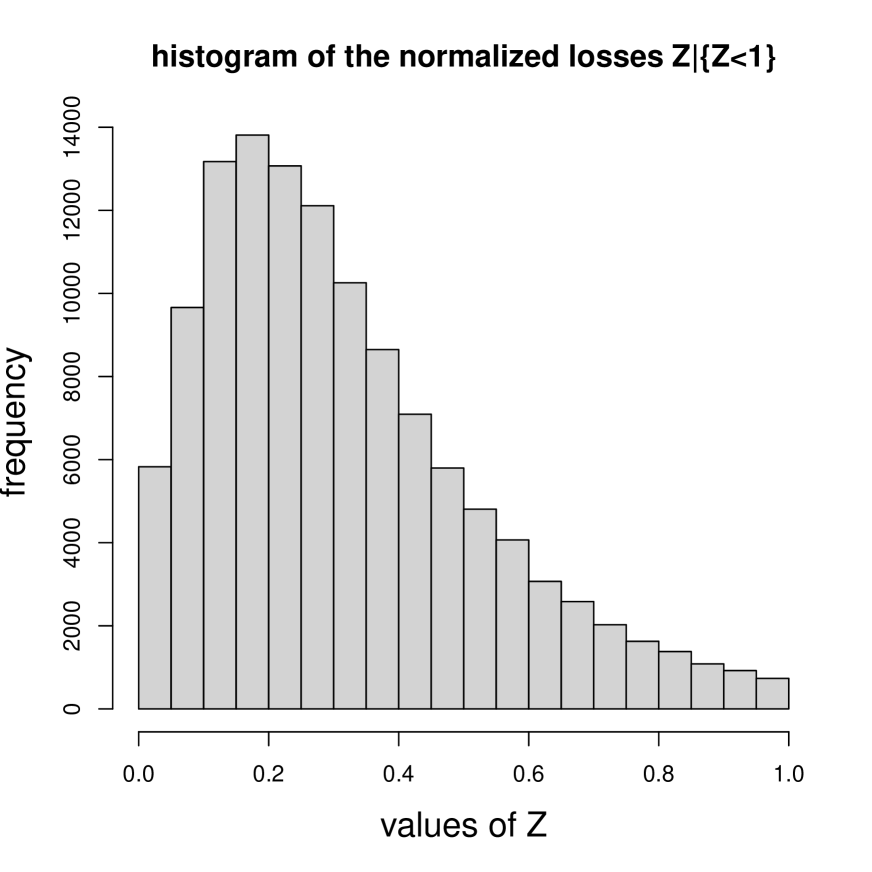
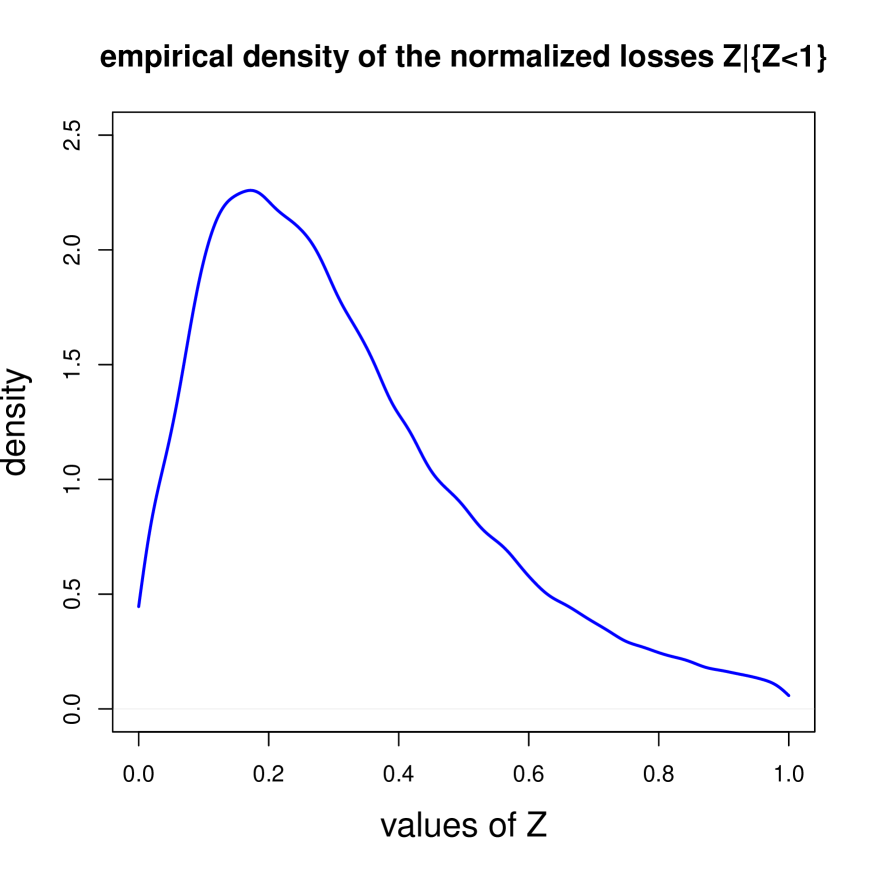
Figure 3: Histogram (lhs) and empirical density (rhs) of the claims $Z_{i}$.

These normalized losses $Z_{i}$, along with different models, will be used to solve the above MLE maximization problems in order to produce the results of this section. For this, we use the R function optim in order to minimize the sum of the negative of the log-likelihoods evaluated at $Z_{i}$, after having possibly transformed our parameters in a way to ensure that they lie in a suitable open domain, as described below. The first fitted model is the classical MBBEFD model of Bernegger [2].

6.1 The MBBEFD example

We have seen in Section 3.3 that the MBBEFD example belongs to the logarithmic linked exposure family and is obtained by choosing

$$b(z)=a+b^{z},$$

for parameters $b\geq 0$ and $a>-\min(1,b)$. Using the parametrization in (3.8), it is possible to give the conditions under which this class of distributions leads to unimodal densities on $[0,1)$. Indeed, according to Proposition 3.2, such unimodal densities are obtained if and only if

$$bg<1\qquad\text{ and }\qquad b<\frac{1-bg}{g-1}<1,$$

for parameters $g>1$ and $b>0$. Therefore, we use the domain

$$\Theta=\Big{\{}g>1,\max\left(0,\frac{2-g}{g}\right)<b<\frac{1}{2g-1}\Big{\}},$$

in order to find unimodal MLE solutions of the standard and extended maximization problems described in (6.1) and (6.2). In Figure 4, the empirical density of the data points strictly smaller than 1 is plotted in blue color. Since this corresponds to a true density integrating to one, we further show the conditional density of $Z|_{\{Z<1\}}$ of the fitted models, using the parameters obtained by solving the standard problem (6.1) (in green) and the extended problem (6.2) (in red). The point mass and the mean are shown in Table 1, as well as the log-likelihoods of the random variables $Z|_{\{Z<1\}}$ and $Z$, and the AIC scores that are computed using $\ell_{Z}$. We see that, as expected, the MLE solution of the extended problem gives better results, even if the densities obtained are not close to the empirical density. Proposition 3.3 helps us to understand why the fit is not accurate since the empirical density is skewed to the right, whereas the MBBEFD class only allows for symmetric densities.

Figure 4: The MBBEFD: densities of the random variable $Z|_{\{Z<1\}}$.

	Point Mass	Mean	$\ell_{Z|_{\{Z<1\}}}$	$\ell_{Z}$	AIC
Empirical density (Blue)	0.034	0.339	-	-	-
MLE of the standard problem (Green)	0.020	0.337	32 682	13 475	-26 947
MLE of the extended problem (Red)	0.034	0.336	33 257	14 587	-29 168

Table 1: The MBBEFD: results.

6.2 Power logarithmic linked exposure example

An example belonging to the logarithmic linked exposure family is obtained by choosing the power function

$$b(z)=\left(1-\frac{z}{\alpha}\right)^{\delta}+a,$$

for $\alpha>1$, $\delta>1$ and a sufficiently large parameter $a>0$. This is a smooth and strictly convex curve on $[0,1]$ with $b(1)=(1-1/\alpha)^{\delta}+a<1+a=b(0)$. The first and second derivatives for $z\in[0,1]$ are given by

$$b^{\prime}(z)=-\frac{\delta}{\alpha}\left(1-\frac{z}{\alpha}\right)^{\delta-1}~{}<~{}0\qquad\text{ and }\qquad b^{\prime\prime}(z)=\frac{\delta(\delta-1)}{\alpha^{2}}\left(1-\frac{z}{\alpha}\right)^{\delta-2}~{}>~{}0.$$

In order to achieve $b^{\prime\prime}(z)b(z)-b^{\prime}(z)^{2}\geq 0$ for all $z\in[0,1]$, which is necessary due to Proposition 4.1, the parameter $a$ has to satisfy

$$a>\max_{z\in[0,1]}\left(\frac{b^{\prime}(z)^{2}}{b^{\prime\prime}(z)}-\tilde{b}(z)\right),$$ (6.3)

where we set $\tilde{b}(z)=\left(1-\frac{z}{\alpha}\right)^{\delta}$. This reads in this example

$$a>\max_{z\in[0,1]}\left(\frac{1}{\delta-1}\left(1-\frac{z}{\alpha}\right)^{\delta}\right)~{}=~{}\frac{1}{\delta-1}.$$ (6.4)

With Corollary 4.2, we then obtain as density for $z\in[0,1)$

$$f_{Z}(z)=\frac{a+1}{\alpha}\frac{\left(1-{z}/{\alpha}\right)^{\delta-2}}{\left(a+(1-{z}/{\alpha})^{\delta}\right)^{2}}\left(a(\delta-1)-\left(1-{z}/{\alpha}\right)^{\delta}\right),$$ (6.5)

with point mass in $z=1$ equal to

$$p=\left(1-\frac{1}{\alpha}\right)^{\delta-1}\frac{a+1}{a+(1-{1}/{\alpha})^{\delta}},$$

and mean

$${\mathbb{E}}[Z]=\frac{\alpha(a+1)}{\delta}\,\log\left(\frac{a+1}{a+(1-{1}/{\alpha})^{\delta}}\right).$$

The derivative of the density $f_{Z}$ is given by

$$f^{\prime}_{Z}(z)=-\frac{a+1}{\alpha^{2}}\,\frac{\left[a^{2}(\delta-1)(\delta-2)-a(\delta-1)(\delta+4)(1-{z}/{\alpha})^{\delta}+2(1-{z}/{\alpha})^{2\delta}\right]}{(a+(1-{z}/{\alpha})^{\delta})^{3}\,(1-{z}/{\alpha})^{-\delta+3}}.$$ (6.6)

Lemma 6.1.

The power logarithmic linked exposure example with the above parameters leads to a well-defined distribution. The density $f_{Z}$ of this power logarithmic linked exposure example given in (6.5) can only be unimodal on $[0,1)$ if $\delta>2$.

Therefore, we use the domain

$$\Theta=\Big{\{}\alpha>1,\delta>2,a>\frac{1}{\delta-1}\Big{\}},$$

in order to find unimodal solutions to the MLE of the standard and extended maximization problems described in (6.1) and (6.2). The results displayed in Figure 5 are very similar to the ones obtained for the MBBEFD example. This can be confirmed by comparing Table 1 and Table 2, where most values coincide although they are actually different if we look at digits after the decimal point.

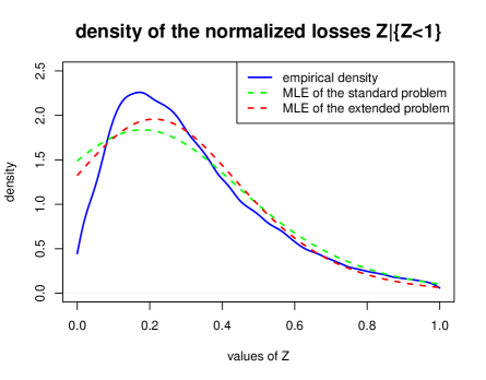
Figure 5: Power logarithmic linked exposure: densities of the random variable $Z|_{\{Z<1\}}$.

	Point Mass	Mean	$\ell_{Z|_{\{Z<1\}}}$	$\ell_{Z}$	AIC
Empirical density (Blue)	0.034	0.339	-	-	-
MLE of the standard problem (Green)	0.020	0.337	32 680	13 475	-26 945
MLE of the extended problem (Red)	0.034	0.336	33 257	14 587	-29 166

Table 2: Power logarithmic linked exposure example: results.

6.3 Sine logarithmic linked exposure example

A third example belonging to the logarithmic linked exposure family is given by the sine function

$$b(z)=\sin(\alpha z+\beta)+a,$$

for $\beta\in\left(-\frac{\pi}{2},0\right),\alpha\in\left(0,\frac{\pi}{2}-\beta\right)$ and $-\sin(\beta)<a<-1/\sin(\beta)$. This is a smooth curve on $[0,1]$ with $b(0)=\sin(\beta)+a<\sin(\alpha+\beta)+a=b(1)$. The first and second derivatives for $z\in[0,1]$ are given by

$$b^{\prime}(z)=\alpha\cos(\alpha z+\beta)~{}>~{}0\qquad\text{ and }\qquad b^{\prime\prime}(z)=-\alpha^{2}\sin(\alpha z+\beta).$$

Note that in this case, the function $b$ is in general neither concave, nor convex on the entire interval $[0,1]$. We claim that the condition $b^{\prime\prime}(z)b(z)-b^{\prime}(z)^{2}\geq 0$ for all $z\in[0,1]$ is fulfilled, which is necessary in order to obtain a distribution function due to Proposition 4.1. Moreover, the density for $z\in[0,1)$ reads

$$f_{Z}(z)=\frac{\sin(\beta)+a}{\cos(\beta)}\,\frac{\alpha\left[1+a\sin(\alpha z+\beta)\right]}{\left[\sin(\alpha z+\beta)+a\right]^{2}},$$ (6.7)

with point mass in $z=1$

$$p=\frac{\cos(\alpha+\beta)}{\cos(\beta)}\,\frac{\sin(\beta)+a}{\sin(\alpha+\beta)+a},$$

and mean

$${\mathbb{E}}[Z]=-\frac{\sin(\beta)+a}{\alpha\cos(\beta)}\,\log\left(\frac{\sin(\beta)+a}{\sin(\alpha+\beta)+a}\right).$$

The derivative of the density $f_{Z}$ is given by

$$f^{\prime}_{Z}(z)=-\frac{\sin(\beta)+a}{\alpha\cos(\beta)}\,\frac{\alpha^{3}\cos(\alpha z+\beta)\left[-a^{2}+a\sin(\alpha z+\beta)+2\right]}{\left[\sin(\alpha z+\beta)+a\right]^{3}}.$$ (6.8)

Lemma 6.2.

The sine logarithmic linked exposure example with the above parameters leads to a well-defined distribution. Moreover, the density $f_{Z}$ given in (6.7) can only be unimodal on $[0,1)$ if $1\leq a\leq 2$.

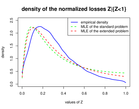
Figure 6: Sine logarithmic linked exposure: densities of the random variable $Z|_{\{Z<1\}}$.

	Point Mass	Mean	$\ell_{Z|_{\{Z<1\}}}$	$\ell_{Z}$	AIC
Empirical density (Blue)	0.034	0.339	-	-	-
MLE of the standard problem (Green)	0.040	0.380	26 907	8 164	-16 323
MLE of the extended problem (Red)	0.034	0.362	30 453	11 783	-23 558

Table 3: Sine logarithmic linked exposure example: results.

We use the domain

$$\Theta=\left\{\beta\in\left(-\frac{\pi}{2},0\right),\alpha\in\left(0,\frac{\pi}{2}-\beta\right),1<a<\min\left(-\frac{1}{\sin(\beta)},2\right)\right\},$$

in order to find unimodal solutions to the standard and extended maximization problems described in (6.1) and (6.2). Similarly as for the previous examples, we obtain the results displayed in Figure 6 and Table 3. Although this example manages to produce rather skewed densities, see Figure 6, the fit does not seem to be accurate for this data, i.e. it is less accurate than in the first examples, and with AIC, we clearly prefer the previous models.

6.4 Quadratic exponentially linked exposure example

Let us now treat an example belonging to the exponentially linked exposure family, and given by the quadratic function

$$b(z)=\alpha z^{2}+\beta z,$$

for $\alpha<0$ and $\beta<-\sqrt{-2\alpha}$. This is a smooth curve on $[0,1]$ with $b(0)=0>\alpha+\beta=b(1)$. The first and second derivatives for $z\in[0,1]$ are given by

$$b^{\prime}(z)=2\alpha z+\beta~{}<~{}0\qquad\text{ and }\qquad b^{\prime\prime}(z)=2\alpha~{}<~{}0.$$

This function $b$ is a smooth and strictly concave curve on $[0,1]$. We claim that the condition $b^{\prime\prime}(z)+b^{\prime}(z)^{2}\geq 0$ is fulfilled for all $z\in[0,1]$, which is necessary in order to obtain a distribution function due to Proposition 5.1. Moreover, the density for $z\in[0,1)$ reads

$$f_{Z}(z)=-\frac{e^{\alpha z^{2}+\beta z}\left[4\alpha^{2}z^{2}+4\alpha\beta z+\beta^{2}+2\alpha\right]}{\beta},$$ (6.9)

with point mass in $z=1$

$$p=\frac{e^{\alpha+\beta}\,[2\alpha+\beta]}{\beta},$$

and mean

$${\mathbb{E}}[Z]=\frac{e^{\alpha+\beta}-1}{\beta}.$$

The derivative of the density $f_{Z}$ is given by

$$f^{\prime}_{Z}(z)=-\frac{e^{\alpha z^{2}+\beta z}\,(2\alpha z+\beta)\left[(2\alpha z+\beta)^{2}+6\alpha\right]}{\beta}.$$ (6.10)

Lemma 6.3.

The quadratic logarithmic linked exposure example with the above parameters leads to a well-defined distribution. Moreover, the density $f_{Z}$ given in (6.9) is unimodal on $[0,1)$ if and only if $-\sqrt{-6\alpha}<\beta<-2\alpha-\sqrt{-6\alpha}$.

We use the domain

$$\Theta=\Big{\{}\alpha<0,\beta\in\left(-\sqrt{-6\alpha}\,,\min\left(-2\alpha-\sqrt{-6\alpha},-\sqrt{-2\alpha}\right)\right)\Big{\}}$$

in order to find unimodal solutions to the standard and extended maximization problems described in (6.1) and (6.2). Similarly as for the previous examples, we obtain the results shown in Figure 7 and Table 4. Although a new family of exposure curves is used here, the results are close to the ones obtained with the power logarithmic linked exposure example or the MBBEFD example. In fact, in the extended problem, we obtain a slightly better model than in the MBBEFD class according to AIC. However, looking at Figure 7, this new model is still not satisfactory for this data.

Figure 7: Quadratic exponentially linked exposure example: densities of the random variable $Z|_{\{Z<1\}}$.

	Point Mass	Mean	$\ell_{Z|_{\{Z<1\}}}$	$\ell_{Z}$	AIC
Empirical density (Blue)	0.034	0.339	-	-	-
MLE of the standard problem (Green)	0.016	0.345	32 101	12 425	-24 846
MLE of the extended problem (Red)	0.034	0.341	33 340	14 726	-29 447

Table 4: Quadratic exponentially linked exposure example: results.

6.5 Power exponentially linked exposure example

Finally, we consider a last example belonging again to the exponentially linked exposure family. This last example is a bit more difficult in handling, but it provides the best results for our example. Choose the power function

$$b(z)=\epsilon(z+\delta)^{\alpha}-\beta z,$$

for $\alpha\in(1,2),\delta>0,\epsilon<0$ and $\beta>\epsilon\alpha\delta^{\alpha-1}+\sqrt{-\epsilon\alpha(\alpha-1)\delta^{\alpha-2}}$. This is a smooth curve on $[0,1]$ with $b(0)=\epsilon\delta^{\alpha}>\epsilon(1+\delta)^{\alpha}-\beta=b(1)$. The first and second derivatives for $z\in[0,1]$ are given by

$$b^{\prime}(z)=\alpha\epsilon(z+\delta)^{\alpha-1}-\beta~{}<~{}0\qquad\text{ and }\qquad b^{\prime\prime}(z)=\alpha(\alpha-1)\epsilon(z+\delta)^{\alpha-2}~{}<~{}0.$$

This function $b$ is a smooth and strictly concave curve on $[0,1]$. We claim that the condition $b^{\prime\prime}(z)+b^{\prime}(z)^{2}\geq 0$ for all $z\in[0,1]$ is fulfilled, which is necessary in order to obtain a distribution function due to Proposition 5.1. Moreover, the density for $z\in[0,1)$ reads as

$$f_{Z}(z)=-\frac{e^{\epsilon(z+\delta)^{\alpha}-\beta z}\left[(\alpha\epsilon(z+\delta)^{\alpha-1}-\beta)^{2}+\alpha(\alpha-1)\epsilon(z+\delta)^{\alpha-2}\right]}{e^{\epsilon\delta^{\alpha}}\left[\alpha\epsilon\delta^{\alpha-1}-\beta\right]},$$

with point mass in $z=1$

$$p=\frac{e^{\epsilon(1+\delta)^{\alpha}-\beta}\,[\alpha\epsilon(1+\delta)^{\alpha-1}-\beta]}{e^{\epsilon\delta^{\alpha}}\,[\alpha\epsilon\delta^{\alpha-1}-\beta]},$$

and mean

$${\mathbb{E}}[Z]=\frac{e^{\epsilon\left[(1+\delta)^{\alpha}-\delta^{\alpha}\right]-\beta}-1}{\alpha\epsilon\delta^{\alpha-1}-\beta}.$$

The derivative of the density $f_{Z}$ can be obtained using (5.6). It does however not allow to characterize the extrema of the density in this example explicitly. Nevertheless, we observe in Figure 8 that this example contains unimodal densities.

Lemma 6.4.

The power exponentially linked exposure example with the above parameters leads to a well-defined distribution.

We use the domain

$$\Theta=\Big{\{}\alpha\in(1,2),\delta>0,\epsilon<0,\beta>\epsilon\alpha\delta^{\alpha-1}+\sqrt{-\epsilon\alpha(\alpha-1)\delta^{\alpha-2}}\Big{\}},$$

in order to find solutions to the standard and extended maximization problems described in (6.1) and (6.2). Similarly as for the previous examples, we obtain the results shown in Figure 8 and Table 5. This time, the fit seems much better. This is especially the case for the red curve, which represents the solution of the flexible maximization problem. The tail behavior on the right and left sides seem adequate in contrast to the plots presented in the previous examples. This observation is confirmed by the AIC scores attained here, which are lower than the AIC scores of all other examples, i.e., we give clear preference to this last example for this data.

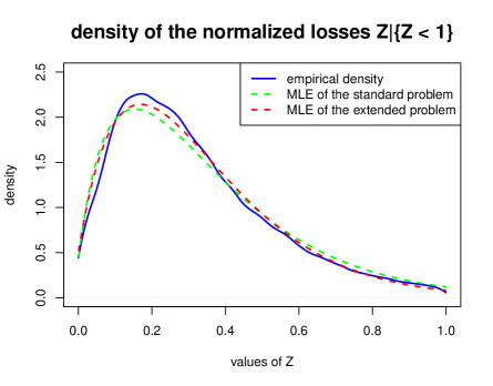
Figure 8: Power exponentially linked exposure example: densities of the random variable $Z|_{\{Z<1\}}$.

	Point Mass	Mean	$\ell_{Z|_{\{Z<1\}}}$	$\ell_{Z}$	AIC
Empirical density (Blue)	0.034	0.339	-	-	-
Standard MLE density (Green)	0.025	0.341	34 068	15 199	-30 390
Flexible MLE density (Red)	0.034	0.339	34 402	15 731	-31 453

Table 5: Power exponentially linked exposure example: results.

7 Conclusion

Most classical statistical models are not directly suited to model lower-truncated and right-censored claims in general insurance since they lead to problems that are not easily analytically tractable. Bernegger introduced in [2] the MBBEFD class of distributions that can model such claims using a distribution function, an absolutely continuous density, and a point mass that are all of closed form. This class was introduced in the reinsurance literature, where densities are typically monotonically decreasing.

In general insurance, however, we are mainly interested in unimodal skewed densities. Therefore, we extended the MBBEFD class to a much bigger family of distributions that we called the Bernegger class. By starting from the properties of an exposure curve, we introduced two subfamilies, namely the logarithmic and exponentially linked exposure curves. Through various examples, we used the full tractability and flexibility of the Bernegger class in order to fit parameters to general insurance claims using maximum likelihood estimations. It turned out that this large class of distributions contains models allowing to obtain a suitable approximation for the distribution of the used dataset, and in general, we have a rich family of unimodal and skewed densities within the Bernegger class. Going forward, it will be interesting to further characterize and classify the members of the Bernegger class based on different properties. Of course, this might involve exploring other link functions. Another next step is to lift these models to regression models allowing for integrating fixed effects described by covariates.

Appendix A Proofs

We prove all statements in this appendix.

Proof of Theorem 2.1. The function $F_{Z}$, as defined in (2.1), is continuously differentiable on the interval $(0,1)$ by our assumptions on $G$. This means that a derivative exists, and is equal to

$$f_{Z}(z)=F_{Z}^{\prime}(z)=-\frac{G^{\prime\prime}(z)}{G^{\prime}(0)}\geq 0,$$

for $z\in[0,1)$. Since $G$ was assumed to be twice continuously differentiable, non-decreasing and concave, we obtain that $0\leq G^{\prime}(z)\leq G^{\prime}(0)$ and $f_{Z}(z)\geq 0$ for all $z\in[0,1]$. This implies

$$0=F_{Z}(0)\leq F_{Z}(z)\leq F_{Z}(1)=1,\,\text{ for all }z\in[0,1].$$

Since $G^{\prime}$ is continuous by assumption, we conclude from (2.1) that $F_{Z}$ is right-continuous, and hence, a distribution function on $[0,1]$. The point mass in 1 is then given by

$$p=1-F_{Z}(1_{-})=\frac{G^{\prime}(1)}{G^{\prime}(0)}\in[0,1],$$

and the mean of $Z\sim F_{Z}$ is equal to

$${\mathbb{E}}[Z]=\int_{0}^{1}1-F_{Z}(s)\,ds=\int_{0}^{1}\frac{G^{\prime}(s)}{G^{\prime}(0)}\,ds=\frac{G(1)-G(0)}{G^{\prime}(0)}=\frac{1}{G^{\prime}(0)}.$$

This proves the theorem.

$\Box$

Proof of Lemma 2.3. First, it is clear that the function $G:[0,1]\rightarrow{\mathbb{R}}$ defined in (2.4) is an exposure curve. Moreover, we have by (2.1) that the distribution function $F_{Z}$ generated by $G$ satisfies

$$\begin{split}F_{Z}(z)&=\left(1-\frac{G^{\prime}(z)}{G^{\prime}(0)}\right)\mathds{1}_{\{z<1\}}+\mathds{1}_{\{z=1\}}\\ &=\left(1-\frac{\sum_{i=1}^{n}\alpha_{i}G_{i}^{\prime}(z)}{\sum_{j=1}^{n}\alpha_{j}G_{j}^{\prime}(0)}\right)\mathds{1}_{\{z<1\}}+\mathds{1}_{\{z=1\}}\\ &=\left(1-\sum_{i=1}^{n}\frac{\alpha_{i}G_{i}^{\prime}(0)}{\sum_{j=1}^{n}\alpha_{j}G_{j}^{\prime}(0)}\frac{G_{i}^{\prime}(z)}{G_{i}^{\prime}(0)}\right)\mathds{1}_{\{z<1\}}+\mathds{1}_{\{z=1\}}\\ &=\left(1-\sum_{i=1}^{n}w_{i}\frac{G_{i}^{\prime}(z)}{G_{i}^{\prime}(0)}\right)\mathds{1}_{\{z<1\}}+\mathds{1}_{\{z=1\}}\\ &=\sum_{i=1}^{n}w_{i}\left(\left(1-\frac{G_{i}^{\prime}(z)}{G_{i}^{\prime}(0)}\right)\mathds{1}_{\{z<1\}}+\mathds{1}_{\{z=1\}}\right)=\sum_{i=1}^{n}w_{i}F_{i}(z),\end{split}$$

for $z\in[0,1]$, and where the elements

$$w_{i}=\frac{\alpha_{i}G_{i}^{\prime}(0)}{\sum_{j=1}^{n}\alpha_{j}G_{j}^{\prime}(0)}~{}\geq~{}0$$

are weights summing up to 1. The proof then follows similarly to Theorem 2.1.

$\Box$

Proof of Proposition 3.2. We calculate the first derivative for $g>1$, $b>0$, $b\neq 1$ and $bg\neq 1$

$$f^{\prime}_{b,g}(z) = -\frac{(g-1)(b-1)(\log(b))^{2}b^{1-z}}{\left((g-1)b^{1-z}+(1-bg)\right)^{2}}+2\frac{(g-1)^{2}(b-1)(\log(b))^{2}b^{2-2z}}{\left((g-1)b^{1-z}+(1-bg)\right)^{3}}$$ (A.1)

$$= \frac{(g-1)(b-1)(\log(b))^{2}b^{1-z}}{\left((g-1)b^{1-z}+(1-bg)\right)^{3}}\left[(g-1)b^{1-z}-(1-bg)\right]$$

$$= (g-1)(b-1)\,(\log(b))^{2}b^{1-z}\,\frac{(g-1)b^{1-z}-(1-bg)}{\left((g-1)b^{1-z}+(1-bg)\right)^{3}}.$$

This derivative can be zero (for $g>1$, $b>0$, $b\neq 1$) if and only if the last ratio is zero.

(a) Case $bg<1$. This implies $1-bg>0$ and $b<1$, and the term in front of the ratio in (A.1) is negative and the denominator in the ratio is positive. In this case, the derivative is thus positive if $0~{}<~{}b^{1-z}~{}<~{}(1-bg)/(g-1)$ and negative if $0<(1-bg)/(g-1)<b^{1-z}$. Since $b^{1-z}$ is increasing in $z$, we have a monotonically increasing density on $[0,1)$ if $(1-bg)/(g-1)\geq 1$ and we have a monotonically decreasing density on $[0,1)$ if $(1-bg)/(g-1)\leq b$. For $b<(1-bg)/(g-1)<1$, we have a unimodal density with critical point

$$z^{*}=1-\frac{\log\left((1-bg)/(g-1)\right)}{\log(b)}~{}\in~{}(0,1).$$

(b) Case $bg=1$. This implies $b<1$. The density $f_{b,g}(z)=-\log(b)b^{z}$ is monotonically decreasing in $z$.

(c) Case $bg>1$. This implies $bg-1>0$. which means that the numerator of the last ratio in (A.1) is thus always positive. We therefore need to analyze for $b\neq 1$ the ratio

$$\frac{b-1}{(g-1)b^{1-z}+(1-bg)},$$

in order to determine the sign of the derivative $f^{\prime}_{b,g}$.

(c1) Consider the first case $b<1$. In this case, we have a negative numerator and $b^{1-z}$ is increasing in $z\in[0,1)$. If $0<b^{1-z}<(bg-1)/(g-1)$, we have an increasing derivative, and for $0<(bg-1)/(g-1)<b^{1-z}$, we have a decreasing derivative. Since in this case, $(bg-1)/(g-1)<b<b^{1-z}$ holds for all $z\in[0,1]$, we have a monotonically decreasing density.

(c2) Consider the second case $b>1$. In this case, we have a positive numerator and $b^{1-z}$ is decreasing in $z\in[0,1)$. If $0<b^{1-z}<(bg-1)/(g-1)$, we have a decreasing derivative, and for $0<(bg-1)/(g-1)<b^{1-z}$, we have an increasing derivative. Since in this case, we have $(bg-1)/(g-1)>b>b^{1-z}$ for all $z\in[0,1]$, the density is decreasing.

Finally, the case $b=1$ also immediately follows. This completes the proof. $\Box$

Proof of Proposition 3.3. For $bg<1$, we have the MBBEFD density

$$f_{b,g}(z) = \frac{(g-1)(b-1)\log(b)b^{1-z}}{\left((g-1)b^{1-z}+(1-bg)\right)^{2}}~{}=~{}\frac{\frac{b(g-1)(b-1)\log(b)}{(1-bg)^{2}}b^{-z}}{\left(\frac{b(g-1)}{1-bg}b^{-z}+1\right)^{2}}$$

$$= \frac{(b-1)\log(b)}{1-bg}\,\frac{\exp\left\{z\log(1/b)+\log\left(\frac{b(g-1)}{1-bg}\right)\right\}}{\left(\exp\left\{z\log(1/b)+\log\left(\frac{b(g-1)}{1-bg}\right)\right\}+1\right)^{2}}.$$

This proves the first claim. For the second claim, we remark that the function $t\mapsto\psi^{\prime}(t)$ is symmetric around the origin $t=0$. In view of our claim, there is $z=z^{*}\in(0,1)$ such that $z\log(1/b)+\log(b(g-1)/(1-bg))=0$ if and only if $b<(1-bg)/(g-1)<1$. Using reparametrization (3.8) completes the proof. $\Box$

Proof of Proposition 4.1. First the function $G(z)$ is well-defined for all $z\in[0,1]$ due to the assumption that the function $b$ maps to the interval $(0,\infty)$ and that $b(0)\neq b(1)$. We compute the first and second derivative of $G$ and obtain

$$G^{\prime}(0) = \frac{b^{\prime}(0)}{b(0)}\,\frac{1}{\log(b(1))-\log(b(0))}~{}>~{}0,$$

$$G^{\prime}(z) = \frac{b^{\prime}(z)}{b(z)}\,\frac{1}{\log(b(1))-\log(b(0))}~{}\geq~{}0,$$

$$G^{\prime\prime}(z) = \frac{b^{\prime\prime}(z)b(z)-b^{\prime}(z)^{2}}{b(z)^{2}}\,\frac{1}{\log(b(1))-\log(b(0))}~{}\leq~{}0,$$

where the inequalities hold if and only if $b^{\prime}(0)>0$, $b^{\prime}(z)\geq 0$ and $b^{\prime\prime}(z)b(z)-b^{\prime}(z)^{2}\leq 0$ for all $z\in[0,1]$, or $b^{\prime}(0)<0$, $b^{\prime}(z)\leq 0$ and $b^{\prime\prime}(z)b(z)-b^{\prime}(z)^{2}\geq 0$ for all $z\in[0,1]$. $\Box$

Proof of Corollary 4.2. According to Theorem 2.1, the function $F_{Z}$ defined in (4.4) satisfies for $z\in[0,1]$

$$\begin{split}F_{Z}(z)&=\left(1-\frac{G^{\prime}(z)}{G^{\prime}(0)}\right)\mathds{1}_{\{z<1\}}+\mathds{1}_{\{z=1\}}\\ &=\left(1-\frac{b^{\prime}(z)}{b^{\prime}(0)}\,\frac{b(0)}{b(z)}\right)\mathds{1}_{\{z<1\}}+\mathds{1}_{\{z=1\}}.\end{split}$$

The remaining statements then follow.

$\Box$

Proof of Proposition 5.1. First the function $G(z)$ is well-defined for all $z\in[0,1]$ due to the assumption that $b(0)\neq b(1)$. We compute now the first and second derivative of $G$ and obtain

$$G^{\prime}(0) = \frac{e^{b(0)}}{e^{b(1)}-e^{b(0)}}\,b^{\prime}(0)~{}>~{}0,$$

$$G^{\prime}(z) = \frac{e^{b(z)}}{e^{b(1)}-e^{b(0)}}\,b^{\prime}(z)~{}\geq~{}0,$$

$$G^{\prime\prime}(z) = \frac{e^{b(z)}}{e^{b(1)}-e^{b(0)}}[b^{\prime}(z)^{2}+b^{\prime\prime}(z)]~{}\leq~{}0,$$

where the inequalities hold if and only if $b^{\prime}(0)>0$, $b^{\prime}(z)\geq 0$ and $b^{\prime}(z)^{2}+b^{\prime\prime}(z)\leq 0$ for all $z\in[0,1]$, or $b^{\prime}(0)<0$, $b^{\prime}(z)\leq 0$ and $b^{\prime}(z)^{2}+b^{\prime\prime}(z)\geq 0$ for all $z\in[0,1]$.

$\Box$

Proof of Corollary 5.2. According to Theorem 2.1, the function $F_{Z}$ defined in (5.4) satisfies for $z\in[0,1]$

$$\begin{split}F_{Z}(z)&=\left(1-\frac{G^{\prime}(z)}{G^{\prime}(0)}\right)\mathds{1}_{\{z<1\}}+\mathds{1}_{\{z=1\}}\\ &=\left(1-\frac{e^{b(z)}}{e^{b(0)}}\frac{b^{\prime}(z)}{b^{\prime}(0)}\right)\mathds{1}_{\{z<1\}}+\mathds{1}_{\{z=1\}}.\end{split}$$

The remaining statements then follow.

$\Box$

Proof of Lemma 6.1. The power logarithmic linked exposure example leads to a well-defined distribution due to (6.3) and Propositon 4.1. Set $y=(1-z/\alpha)^{\delta}\in((1-1/\alpha)^{\delta},1]$ for $z\in[0,1)$. The derivative (6.6) is zero only if

$$a^{2}(\delta-1)(\delta-2)-a(\delta-1)(\delta+4)y+2y^{2}=0.$$

If there exist real-valued solutions, they are given by

$$y_{\pm} = a\,\frac{(\delta-1)(\delta+4)\pm\sqrt{(\delta-1)^{2}(\delta+4)^{2}-8(\delta-1)(\delta-2)}}{4}.$$ (A.2)

We start with the case $\delta\in(1,2]$. In that case, we have

$$(\delta-1)(\delta+4)\leq\sqrt{(\delta-1)^{2}(\delta+4)^{2}-8(\delta-1)(\delta-2)}.$$

This implies for the smaller solution $y_{-}\leq 0$, thus, this solution provides $y_{-}\not\in((1-1/\alpha)^{\delta},1]$. For the bigger solution, we have, using (6.4) in the second step,

$$y_{+}\geq a\,\frac{(\delta-1)(\delta+4)}{4}>\frac{\delta+4}{4}>1.$$ (A.3)

Thus, also this second solution provides $y_{+}\not\in((1-1/\alpha)^{\delta},1]$, therefore the density is monotone for $\delta\in(1,2]$.

Next, we analyze the case $\delta>2$. The term under the square root in (A.2) is given by

$$(\delta-1)^{2}(\delta+4)^{2}-8(\delta-1)(\delta-2) = (\delta-1)\left[(\delta-1)(\delta+4)^{2}-8(\delta-2)\right]$$

$$= (\delta-1)\left[(\delta-1)(\delta^{2}+8\delta+8)+8\right]~{}>~{}0.$$

Thus, there are two real-valued solutions to (A.2). The bigger solution $y_{+}$ also provides (A.3), and henceforth, $y_{+}\not\in((1-1/\alpha)^{\delta},1]$. Therefore, we can focus on the smaller solution $y_{-}$. It is given by

$$y_{-} = a(\delta-1)\left[(\delta/4+1)-\sqrt{(\delta/4+1)^{2}-\frac{\delta-2}{2\delta-2}}\right].$$

The square bracket is in $[0,0.1]$, therefore there are $\alpha>1$ and $a>1/(\delta-1)$ such that $y_{-}\in((1-1/\alpha)^{\delta},1]$. In particular, there is a critical point $z^{*}\in(0,1]$ with $f_{Z}(z^{*})=0$ in these cases and we easily see from (6.6) that $z^{*}$ is a maximum. This does however not hold for any $\alpha>1$ and $a>1/(\delta-1)$. $\Box$

Proof of Lemma 6.2. In order to prove that the sine logarithmic linked exposure example leads to a well-defined distribution function, we need to show that the function $h$ defined through $h(z)=b^{\prime\prime}(z)b(z)-b^{\prime}(z)^{2}$ satisfies $h(z)\leq 0$ for all $z\in[0,1]$ according to Proposition 4.1. For this, it suffices to show that $h(0)\leq 0$ and $h^{\prime}(z)\leq 0$ for any $0\leq z\leq 1$. This indeed holds since

$$\begin{split}h(0)&=b^{\prime\prime}(0)b(0)-b^{\prime}(0)^{2}\\ &=-\alpha^{2}\sin(\beta)\Big{[}\sin(\beta)+a\Big{]}-\Big{[}\alpha\cos(\beta)\Big{]}^{2}\\ &=-\alpha^{2}[1+a\sin(\beta)]~{}<~{}0,\end{split}$$

where the last inequality is due to $a<-\frac{1}{\sin(\beta)}$. Furthermore, let $z\in[0,1]$, then

$$\begin{split}h^{\prime}(z)&=b^{\prime\prime\prime}(z)b(z)-b^{\prime}(z)b^{\prime\prime}(z)\\ &=-\alpha^{3}\cos(\alpha z+\beta)\Big{[}\sin(\alpha z+\beta)+a\Big{]}-\alpha\cos(\alpha z+\beta)(-\alpha^{2}\sin(\alpha z+\beta))\\ &=-a\alpha^{3}\cos(\alpha z+\beta)~{}<~{}0,\end{split}$$

since $a>0$, $\alpha>0$ and $\alpha z+\beta\in(-\frac{\pi}{2},\frac{\pi}{2})$ for any $z\in[0,1]$. From (6.8), we see that this derivative has either no root or a unique root $z^{*}\in[0,1]$ satisfying

$$z^{*}=\frac{1}{\alpha}\left[\sin^{-1}\Big{(}\frac{a^{2}-2}{a}\Big{)}-\beta\right],$$ (A.4)

where the inverse function $\sin^{-1}(\cdot)$ is chosen to map to the interval $[-\frac{\pi}{2},\frac{\pi}{2}]$. This root can only exist if $-2\leq a\leq-1$ or $1\leq a\leq 2$. Since $a$ was assumed to be positive, this means that the density $f_{Z}$ can only be unimodal when $1\leq a\leq 2$. Note that this condition is not sufficient since we do not a priori obtain that there is a root $z^{*}$ lying in the interval $(0,1)$. However, in the case where this root $z^{*}\in(0,1)$ exists, it is clear from (6.8) that it corresponds to a maximum of the density.

$\Box$

Proof of Lemma 6.3. The function $b$ of this example is strictly decreasing, which means that the necessary condition in order to obtain a well-defined distribution reads $b^{\prime\prime}(z)+b^{\prime}(z)^{2}\geq 0$ for all $z\in[0,1]$ according to Proposition 5.1. This condition holds due to the assumption $\beta<-\sqrt{-2\alpha}$. Furthermore, the roots of the derivative of the density in (6.10) are given by solving

$$2\alpha z+\beta=0\quad\textrm{or}\quad(2\alpha z+\beta)^{2}+6\alpha=0.$$

Note that by the conditions imposed on the parameters, we have $2\alpha z+\beta<0$ for all $z\in[0,1]$. This means that the only extrema in the interval $[0,1]$ can lie at

$$z_{-}=\frac{-\beta-\sqrt{-6\alpha}}{2\alpha}\quad\textrm{and}\quad z_{+}=\frac{-\beta+\sqrt{-6\alpha}}{2\alpha}.$$

Furthermore, since $\alpha<0$ and $\beta<0$, we obtain $z_{+}<0$. This means that the density can have at most one extremum $z^{*}$ lying between 0 and 1, and we have that $z^{*}\in(0,1)\iff 0>-\beta-\sqrt{-6\alpha}>2\alpha$, which is equivalent to $-\sqrt{-6\alpha}<\beta<-2\alpha-\sqrt{-6\alpha}$. Note finally that this extremum $z^{*}\in(0,1)$ corresponds to the maximum of the density due to (6.10).

$\Box$

Proof of Lemma 6.4. Since the function $b$ of this example is strictly decreasing, the necessary condition in order to obtain a well-defined distribution reads $b^{\prime\prime}(z)+b^{\prime}(z)^{2}\geq 0$ for all $z\in[0,1]$ according to Proposition 5.1. This condition holds due to the assumptions made on the different parameters. Indeed, these assumptions imply that $b^{\prime}(z)$ is decreasing, while $b^{\prime\prime}(z)$ is increasing for all $z\in[0,1]$. This means in particular that $b^{\prime\prime}(z)+b^{\prime}(z)^{2}$ is increasing for all $z\in[0,1]$. In order to prove the above necessary condition, it thus suffices to show that

$$b^{\prime\prime}(0)+b^{\prime}(0)^{2}>0.$$

Given that $\alpha>0$, $\delta>0$ and $\epsilon<0$, this is equivalent to

$$\alpha(\alpha-1)\epsilon\delta^{\alpha-2}+(\alpha\epsilon\delta^{\alpha-1}-\beta)^{2}>0\iff\left|\alpha\epsilon\delta^{\alpha-1}-\beta\right|>\sqrt{-\alpha(\alpha-1)\epsilon\delta^{\alpha-2}}.$$

Let us first assume that $\beta>\alpha\epsilon\delta^{\alpha-1}$, which is necessary in order to obtain $b^{\prime}(z)<0$ for all $z\in[0,1]$. This implies that the interior of the absolute value is negative, we can thus write

$$\begin{split}b^{\prime\prime}(0)+b^{\prime}(0)^{2}>0&\iff\beta-\alpha\epsilon\delta^{\alpha-1}>\sqrt{-\alpha(\alpha-1)\epsilon\delta^{\alpha-2}}\\ &\iff\beta>\alpha\epsilon\delta^{\alpha-1}+\sqrt{-\alpha(\alpha-1)\epsilon\delta^{\alpha-2}}.\end{split}$$

The parameter $\beta$ needs thus to satisfy precisely this last condition in order to obtain a well-defined distribution function.

$\Box$

References

- [1] Abramson, D. (2022). A nonproportional premium rating method for construction risks. North American Actuarial Journal 26/4, 626-645.
- [2] Bernegger, S. (1997). The Swiss Re exposure curves and the MBBEFD distribution class. ASTIN Bulletin 27/1, 99-111.
- [3] Blæsild, P., Jensen, J.L. (1985). Saddlepoint formulas for reproductive exponential models. Scandinavian Journal of Statistics 12/3, 193-202.
- [4] Dutang, C., Gesmann, M., Spedicato, G. (2021). Exposure rating, destruction rate models and the mbbefd package. R Vignettes.
- [5] Fung, T.C., Badescu, A.L., Lin, X.S. (2022). Fitting censored and truncated regression data using the mixture of experts models. North American Actuarial Journal, 26/4, 496-520.
- [6] Landsman, Z., Valdez, E.A. (2005). Tail conditional expectation for exponential dispersion models. ASTIN Bulletin 35/1, 189-209.
- [7] Parodi, P. (2014). Pricing in General Insurance. CRC Press.
- [8] Parodi, P., Watson, P. (2019). Property graphs - a statistical model for fire and explosion losses based on graph theory. ASTIN Bulletin 49/2, 263-297.
- [9] Poudyal, C. (2021). Robust estimation of loss models for lognormal insurance payment severity data. ASTIN Bulletin 51/2, 475-507.
- [10] Poudyal, C. (2021). Truncated, censored, and actuarial payment-type moments for robust fitting of a single-parameter Pareto distribution. Journal of Computational and Applied Mathematics 388, 113310.
- [11] Poudyal, C., Brazauskas, V. (2022). Robust estimation of loss models for truncated and censored severity data. Variance 15/2.
- [12] R Core Team (2018). R: A language and environment for statistical computing. R Foundation for Statistical Computing, Vienna, Austria. https://www.R-project.org/
- [13] Riegel, U. (2010). On fire exposure rating and the impact of the risk profile type. ASTIN Bulletin 40/2, 727-777.
- [14] Spedicato, G.A., Dutang, C. (2015). The mbbefd package: a package for handling destruction rates in R including MBBEFD distributions. R Vignettes.
- [15] Tweedie, M.C.K. (1984). An index which distinguishes between some important exponential families. In: Statistics: Applications and New Directions. Ghosh, J.K., Roy, J. (Eds.). Proceeding of the Indian Statistical Golden Jubilee International Conference, Indian Statistical Institute, Calcutta, 579-604.
- [16] Verbelen, R., Gong, L., Antonio, K., Badescu, A., Lin, S. (2015). Fitting mixtures of Erlangs to censored and truncated data using the EM algorithm. ASTIN Bulletin 45/3, 729-758.
- [17] Wüthrich, M.V., Merz, M. (2023). Statistical Foundations of Actuarial Learning and its Applications. Springer Actuarial. https://link.springer.com/book/10.1007/978-3-031-12409-9