The greatest GOES soft X-ray flares: Saturation and recalibration over two Hale cycles

1 Introduction

sec:intro

The A,B,C,M,X soft X-ray (SXR; 1-8 Å) flare classification system based on observations by the Geostationary Operational Environmental Satellite (GOES) network has become the standard measure of solar flare strength. These data come from the X-ray Sensor (XRS) instruments on board these satellites, and in this paper we routinely refer to GOES/XRS data as simply GOES data. The classification scheme is defined as follows: GOES classes A1-9 through X1-9 correspond to flare peak 1-8 Å fluxes of $(1-9)\times 10^{n}$ Wm^-2 where $n=[-8,-7,-6,-5,-4]$, for classes A, B, C, M, and X, respectively. Occasionally, flares are observed with peak fluxes $\geq 10^{-3}$ Wm^-2. Rather than being assigned a separate letter designation, such flares are referred to as $\geq$X10 events; it is these few events (often “saturated” ones) that we focus on here. Traditionally, the peak-flux class assigned a given event comes from the largest one-minute average of the flare’s time profile without correction for background.

Prior to the GOES spacecraft (the first of the series launched in 1975), similar flare soft X-ray measurements were initiated on a series of SOLRAD and other early spacecraft such as the two SMS satellites, beginning as early as 1963 (Kahler and Kreplin, 1991). Neupert (2011) describes the earlier GOES data and the intercalibration issues of the GOES spacecraft up through GOES-14. We do not include any of the related data from missions prior to GOES-1 in our present treatment for various reasons (weak metadata, inaccessibility, technology differences, database incompleteness, etc.). During the long history of the GOES/XRS instruments, the two major technical changes were the switch from spin-stabilized to 3-axis spacecraft with GOES-8 (Hanser and Sellers, 1996), and the detector change from ion chambers to Si photodiodes beginning with GOES-16 (Chamberlin et al., 2009; Machol et al., 2020).

In the switch from spin-stabilized satellites to 3-axis-stabilized satellites, the XRS measurements were found to disagree, with GOES-8 through GOES-15 measuring higher irradiances than the preceding instruments. To maintain consistency with previous satellites, the NOAA Space Weather Prediction Center (SWPC) used “SWPC scaling factors” to adjust the GOES-8 through GOES-15 XRS measurements to match the previous measurements (Machol et al., 2022, provide a full description of this). These corrections were applied to all GOES-8 through GOES-15 XRS measurements and are commonly known as the “SWPC scaling factors”. Based on careful pre-launch calibrations of the GOES-16 and GOES-17 XRS instruments, NOAA determined that the GOES-8 through GOES-15 instruments had the correct calibrations, and upward scaling should have instead been applied to the earlier GOES-1 through GOES-7 satellites. For GOES-8 through GOES-15, NOAA’s operational GOES irradiances and flare classifications have used XRS data with the SWPC scaling factor applied, resulting in flare magnitudes that are approximately 40% lower than the modern correct values. To properly calibrate GOES-1 through GOES-15 irradiances as reported prior to these corrections, all irradiances for operational GOES-1 through GOES-15 should thus be multiplied by a scaling factor of 1.43 and the flare classifications should correspondingly be adjusted to match the irradiances. Reprocessing of a new science-quality version of the GOES-1 through GOES-15 data with the calibration corrected is underway at the NOAA National Centers for Environmental Information (NCEI); it is complete for GOES-13 through GOES-15 at the time of writing and will be fully implemented in 2023 for the earlier satellites, making the eventual database consistent with the current GOES-R series. This paper only deals with XRS Channel–B data (1–8 Å), and concludes with a table of events at $\geq$X10 in this corrected modern scale.

Since the beginning of GOES SXR observations in 1975, there had been 22 events listed with a classification $\geq$X10.0, and (depending upon epoch) such events may have driven the sensors’ readings into saturation. The greatest such event, SOL2003-11-04, was assigned an estimated peak value of X28, though it saturated at the X18.4 level. The earlier SOL2003–10–28 event saturated only slightly at the X18.4 level in GOES-10 (but did not saturate at X17.2 in GOES-12) and probably served as a template for the class of the bigger event (Kiplinger and Garcia, 2004).

Given the susceptibility of our electronic infrastructure to space weather (e.g., Cannon, 2013; Hapgood et al., 2021), the magnitudes of the most powerful GOES SXR flares have great practical interest. While the 1-8 Å  SXR band contains only $\leq 2$% of the flare radiative or bolometric energy (Woods, Kopp, and Chamberlin, 2006), the GOES SXR class correlates (but not linearly) with estimates of the total flare radiative energy (Kretzschmar, 2011). The GOES class also can be used as an indicator of the potential impact of associated geomagnetic storms and solar energetic proton (SEP) events – “potential,” because the effects of these phenomena depend on considerations other than flare magnitude, e.g., the occurrence of an associated coronal mass ejection (CME) and location of the flare on the Sun for both storms and (SEP) events and the direction of the magnetic field in the CME for magnetic storms. Moreover, the fact that the saturated GOES events constitute the high-energy tail of the occurrence distribution function (ODF) of these bursts makes them critical for extrapolation of the ODF to larger peak fluxes. The threat of solar “superflares” at this extreme end of the distribution has rightly attracted great interest (e.g., Cliver et al. 2022), and improved values will inform the 100–year extreme-event Benchmarking exercise carried out by the US Space Weather Operations, Research, and Mitigation Subcommittee (SWORM 2018, IDA 2019). In this study we incorporate our revised fluxes for the 12 saturated GOES SXR flares (from 1978 to the present) to assess the ODF across its entire range.

In this paper we analyze GOES/XRS only on the basis of the existing user database as extracted via the the common data environment SolarSoft (Freeland and Handy, 1998) (Section sec:db), and only for the 1–8 Å channel (XRS–B, low photon energy, long wavelength). In Section sec:corrections, we describe and implement our techniques for estimating peak 1–8 Å fluxes for the saturated flares and in Section sec:ofd we incorporate these revised values in the cumulative frequency distribution of peak fluxes for the entire flare GOES database since 1975. This represents the first complete sample of this standard proxy to total flare energy, with significance not only for space weather but also for analogous stellar events. In the Appendix we provide adjusted classes for the most energetic events, accurate to an estimated 20%.

2 Database

sec:db

2.1 History and recalibration

sec:recal

Over the decades of GOES/XRS data, the instrumentation had evolved only slightly up until the GOES-R series (the current GOES-16, GOES-17, and GOES-18 at present, and GOES–19 in the future; Machol et al., 2020). The GOES sensors, both current and earlier, essentially integrate all of the incident or ambient ionizing radiation. This includes not only solar X–rays but any other source of ionization in the satellite environment. The GOES-R (Chamberlin et al., 2009) solid-state photodiodes have closely similar X-ray responses but substantially different background properties, including greater sensitivity to ambient fluxes of energetic electrons. Thomas, Starr, and Crannell (1985), Garcia (1994), and White, Thomas, and Schwartz (2005) definitively discuss the calibration issues of GOES data up through GOES-12, including a detailed treatment of the effects of spectral model uncertainties such as elemental abundances in thermal emission spectra. GOES-13 through GOES-17 data come from https://www.ngdc.noaa.gov/stp/satellite/goes-r.html, which includes several different background levels. In this paper we uniformly used our own algorithm for individual flare background estimates. These earlier papers do not discuss the calibration effect of the change from spin–stabilization to three–axis stabilization between GOES-7 and GOES-8, an example of the systematic issues that remain open at present (see Neupert, 2001, who remarks that the spectral response functions for the spin–stabilized instruments do, however, incorporate the geometry of the scanning motion).

Our approach here is to analyze the irradiance data that NOAA make available at the time of writing, rather than to work with the original raw data (“counts,” or raw digital signal levels) and attempt a comprehensive re-calibration. Indeed, much of this primary data has not been preserved. The database work begins with event identification via the NOAA text files created incrementally in near real time and available on the Web. We then used the SolarSoft ogoes software to access the recalibrated data for each event, noting that the GOES-1 through GOES-15 data now include further cleaning, reflagging, and correction for temperature and digization issues. The geosynchronous orbits of the GOES satellites result in a very high duty cycle, which exceeds 90% even early in the program, and recently is near 100%, with overlapping data streams from the three new-series GOES-R spacecraft at present. Figure fig:history shows the time ranges of the various GOES spacecraft.

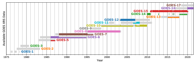
Figure 1.: History of GOES/XRS data availability covering 1975 to 2022, showing primary (colored) and secondary (gray-shaded) sources where this information is available (from Machol et al., 2022). fig:history

We have carried out a systematic intercomparison of overlapping GOES data streams, as summarized in Figure fig:rats_plot. Not all such possible pairs existed, especially at earlier times. This exercise essentially intercompares the independent absolute calibrations, as carried out prior to launch, of each of the spacecraft. The GOES-16/GOES-15 ratio compares the newer and older detector technology, and the “G16/G15” point on the plot shows a ratio $1.10\pm 0.04$ based on peak fluxes in the 1-8 Å channel for 243 $\geq$C-class flares from occurring in 2017 to mid-2019.

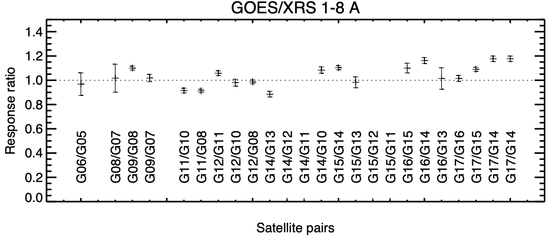
Figure 2.: The average ratios of different pairs of GOES/XRS 1–8 Å peak fluxes derived from simultaneous overlapping observations, using only events at the C1 level and above. Here “G06” stands for “GOES-6”, etc. The uncertainty flags show the standard deviations of the mean ratio. fig:rats˙plot

Based on these comparisons, we conclude that the GOES radiometry has remained roughly stable over the decades, and the data have remained generally intercomparable from instrument to instrument to within about 20%. At this level of absolute calibration, we believe that future refinements and adjustments of the database will not significantly affect the conclusions we draw regarding the ODF.

The NOAA reports, in the text files noted above, defined the original ABCMX classifications. These reports have many blemishes and ambiguities, and some systematic issues. The NOAA text files (Flare Reports) also do not remove the scaling factor. We note that NOAA plans to make corrected scalings available in these reports, extending back to GOES-1, in 2023. Notably the classifications systematically overestimate the irradiances of the flares themselves, because they do not correct for the solar background signal levels. This makes them unsuitable for physical analysis, as noted by Bornmann (1990) and others. Our analysis of the data includes event-by-event background corrections in order to avoid this issue. This work thus parallels that of Aschwanden and Freeland (2012), though with a different algorithm and with an additional decade of data accumulation (see also Sakurai, 2022). While doing this background correction, we have also tried to eliminate as many as possible of the errors in the database as well, making checks to reject outliers in various parameters.

For each event in the NOAA listing, we retrieved the full-resolution data from the source identified by the ogoes tool in SolarSoft, using a fixed time window starting 1800 s prior to the NOAA listing of peak time for each flare, and continuing for 600 s afterwards. At the time of writing, this access tool returns data that have the scaling factor removed for GOES-13 through GOES-15, but the earlier listings require the scaling factor to be removed manually until the NCEI repository is updated.

We estimate the peak time and peak flux from the fine sampling of the data (at 3-s, 2-s, and 1-s intervals depending on spacecraft), after finding background intervals algorithmically. The algorithm locates a minimum level, usually in the half hour prior to the flare peak, for each flare. Note that our use of the full time resolution available makes our numbers slightly inconsistent with earlier descriptions based on 1-minute averages. We do this to improve (slightly) the physical significance of the results, noting that the background corrections have a more important systematic effect. This comparison required screening against outliers, bringing the total number of C-class and greater down from 56,356 to 48,131– a reduction of about 15% – covering the events from SOL1975-09-01T15:12 to SOL2022-06-15T07:25. This cleaning-up of the database included visual inspection of all of the X-class events (as originally labeled), rejecting flawed data from which reasonable assessment of peak or background level could not be made, and the the case-by-case background correction. We note also that the scale corrections and the variability of the background levels confuse the identification of C-class flares (see Fig. 12 of Hudson, 2021, and its accompanying explanation).

2.2 Correction of flare classifications for saturated events

sec:corrections

The database contains 22 events at the $\geq$X10 level, of which 12 had saturated peak flux levels (clipped peaks) in the 1-minute high-resolution 1-8 Å Channel B data (note the 0.5-4 Å Channel A also saturated in a different and overlapping set of events, but we are not considering these data in our analysis). The “saturation” we see in these 12 events (all prior to GOES-13) comes from the readout electronics, specifically in the range limit of digitization of the basic analog measurements. We have no reason to suspect non-linearity of the analog signal near the digital thresholds, which vary from satellite to satellite. The actual conversion from detector currents to physical units requires knowledge of the spectral distribution, which differs from flare to flare; this leads to some unavoidable systematic error (e.g., Wende, 1972). The XRS readouts on the GOES-R (GOES-16 through GOES-18) satellites have a broader dynamic range than those on the earlier satellites, and so will not experience saturation events as easily. For instance, the XRS-B channel on GOES-16 will only saturate for an $\geq$X500 flare (at which point there are other things to worry about!).

We have used two techniques to make plausible extrapolations to determine best values for the peak fluxes of these events, testing our methods against artificially truncated X10-class flares for which we have complete time series; the database for this verification activity contains 10 such events (Table tab:test). The GOES data sampling for these events is is nominally 3-s (with sporadic intermittent occurrences of 2 and 4 s and occasional short gaps of  10 s between data points), and we have used this resolution to estimate the peak values using two methods. The linear method, arrived at by visual trial and error, crudely extrapolates the pre- and post-saturation time series (over 30-s intervals) at their full time resolution via linear extensions, determining the peak flux by the value at the intersections of these two lines. The alternative functional method makes use of a specific parametrized function, fitted by eye in each case. We emphasize that both methods are necessarily subjective, as with earlier similar efforts (e.g., Kiplinger and Garcia, 2004); here the common assumption between our two methods is that they rely upon the slopes of the light curve just before and just after the interval of saturation.

Table 1.: Test Eventstab:test

Event peak time	Class∗	Cut∗	Linear	Functional	Satellite
SOL1982-06-06T16:37	X10.1	X5	X9.3	X8.4	GOES-2
SOL1982-12-15T02:02	X12.9	X5	X10.0	X9.0	GOES-2
SOL1982-12-17T18:57	X10.1	X5	X8.4	X8.2	GOES-2
SOL1984-05-20T22:36	X10.1	X5	X9.2	X9.2	GOES-5
SOL1991-01-25T06:34	X10.8	X5	X10.0	X10.7	GOES-6
SOL1991-06-09T01:43	X10.5	X5	X9.8	X8.0	GOES-6
SOL2001-04-15T13:49	X15.9	X8	X16.0	X16.4	GOES-10
SOL2003-10-28T11:10	X18.6a	X9	X16.2	X16.0	GOES-10
SOL2003-10-29T20:49	X10.9b	X5	X10.9	X10.7	GOES-10
SOL2005-09-07T17:40	X18.1c	X9	X19.7	X16.9	GOES-12

^∗Determined from 3-s data
^aSaturated at $\sim$X18.4 for 1.4 min
^bSaturated at $\sim$X10.9 for $\sim$40 s
^cBlended time profile above saturation level?

2.2.1 Linear fits

This method relies on bridging the gap between the last and first good measurements at the ends of the saturation interval, by upward linear extrapolation of the last part of the flare rise curve prior to saturation, and the first part of the flare rise curve after saturation extrapolated to their point of intersection.

To see if this method had validity, we first tried it by artificially truncating the time profiles of a sample of large (near X10 or greater) GOES events (Table tab:test) at a level of about half the peak flux and then manually extrapolating from the remaining profiles on either side of the “saturation” gap to a peak flux. When this simple method showed promise – the estimated peaks were reasonably close to the actual values – we followed a more quantitative and reproducible approach:

1. fit a straight line through the last 30 seconds (10 data points) prior to saturation of the rise portion of an event;

2. do the same for the first 30 seconds data points after saturation on the decay;

3. extrapolate both lines upward until they intersect; and thence

4. obtain a one-minute average for the 20 highest data points contiguous to the point of intersection.

This procedure is illustrated for SOL1991-01-25 in Figure fig:f1 (left) and the results for all 10 events are given in the “linear” column of Table tab:test. In general the slope on the rise time is too steep (because it does not allow for the decrease of the rise rate as one approaches the peak) and too shallow on the decay which is typically more exponential. These two errors can be somewhat offsetting, resulting in an earlier and more distinct peak which tends to precede that of the actual flare. In the Table it can be seen that the estimated peaks range from 78% to 109% of the actual peaks with a median value of 92%. Figure fig:f1 (right) shows that the method can fail if the time profile exhibits complexity above the saturation level; SOL2005-09-07 was the only event with a ratio of the estimated-to-actual peak flux significantly greater than unity via this method.

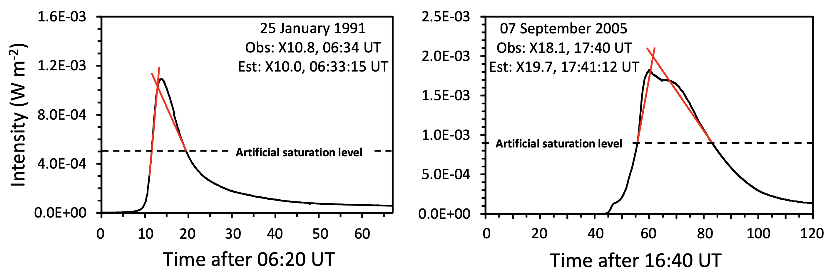
Figure 3.: Left, estimation of flare GOES class (X9.9) for an artificially saturated X10.8 flare SOL1991-01-25. Right, estimation of flare GOES class (X19.7) for an artificially saturated X18.0 event SOL2005-09-07. Here the flare complexity compromises the peak estimation. fig:f1

The linear-fit results for the 12 flares that actually saturated the GOES detector are given in Table tab:meth. For five of these events the estimated peak value is a factor of 1.5-2 larger than the nominal (archived) value. For SOL2003-11-04 we obtained a revised classification of X30.5. This approach (the linear fit) is similar to that of Kiplinger and Garcia (2004) who obtained a peak of X30.6. In an abstract of an AAS talk, Kiplinger and Garcia (2004) mention comparing the time profile of this event with other flares from the “Halloween” episode region (NOAA 10486; Gopalswamy et al., 2005) that produced SOL2003-11-04; note that our methods do not attempt to use common properties of homologous flares in this way. Cliver and Dietrich (2013) had previously combined the Kiplinger and Garcia X30.6 classification with peak fluxes inferred from sudden ionospheric disturbances for this event (e.g., Thomson, Rodger, and Clilverd, 2005) to obtain a GOES classification of X35$\pm$5. The Kretzschmar-Schrijver relationship between flare total solar irradiance and GOES class yields an $\sim$X35 classification for this flare based on its bolometric energy of $4.3\times 10^{32}$ erg (Emslie et al., 2012; Cliver et al., 2022). From the linear analysis of the events in Table tab:test, we would expect the inferred values to be about 10% lower on average than the unknown true values and our peak times to be 1-2 minutes earlier. The  10% underestimates of peak GOES fluxes given by the linear method make it a conservative approach for the reconstruction of the high-flux end of the ODF described in Section sec:ofd below.

Table 2.: Saturated Eventstab:meth

Event	Satellite	Class∗	Maximum	Duration	Linear	Functional
			10${}^{-4}~{}$Wm-2	mm:ss	Class	Class
SOL1978-07-11	GOES-2	X15	1.57	11:05	X31.2	X33.1
SOL1984-04-24	GOES-5	X13	1.30	3:42	X13.9	X13.7
SOL1989-03-06	GOES-6	X15	1.18	7:06	X13.5	X13.2
SOL1989-08-16	GOES-6	X20	1.16	32:23	X20.5	X18.8
SOL1989-10-19	GOES-6	X13	1.16	19:32	X17.0	X15.4
SOL1991-06-01	GOES-6	X12	1.16	26:38	X20.1	X19.6
SOL1991-06-04	GOES-6	X12	1.16	20:31	X23.1	X21.7
SOL1991-06-06	GOES-6	X12	1.16	16:19	X23.1	X19.2
SOL1991-06-11	GOES-6	X12	1.16	3:04	X12.0	X11.9
SOL1991-06-15	GOES-6	X12	1.16	11:38	X25.3	X23.3
SOL2001-04-02	GOES-10	X20	1.84	4:12	X21.4	X20.1
SOL2003-11-04	GOES-10	X28	1.84	13:36	X30.5	X30.0

^∗https://www.ngdc.noaa.gov/stp/space-weather/solar-data/solar-features/solar-flares/x-rays/goes/xrs/

2.2.2 Functional fits

sec:functional

Because of the simplicity of the linear fits, we repeated the curve-fitting exercise across the data gaps in the saturated events, now using a functional form more representative of flare soft X-ray time profiles. Thus we fitted a smooth-topped characteristic function described by

$$\ilabel{eq:function}F(t)=A\,(1-e^{-\Delta t/\tau_{1}})\,e^{-\Delta t/\tau_{2}}\ \ ,$$ (1)

with $\Delta t$ measured relative to an adjustable reference time $\tau_{0}$, nominally the peak time as determined by a bisector method. This is basically a four-parameter fitting procedure, applied manually with reference to subjective goodness-of-fit to the function. Because of the rounded peak, we would expect to find slightly lower peak fluxes this way, and this is indeed the case, with the median estimated peaks ranging from 70% to 103% of the actual peaks, with a median value of 89%. Figure fig:functional_fit_plots shows the timeseries for the two events shown in Figure fig:f1.

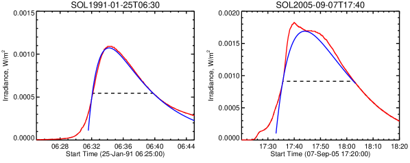
Figure 4.: Time series for 1-8 Å for the same two reference events shown in Figure fig:f1, but now with the functional fits (Equation eq:function) superposed (blue) on the artificially truncated GOES data (red). The right panel (SOL2005-09-07) shows a case with an error in peak flux of about 8%, and a 3-min miss in time of peak. fig:functional˙fit˙plots

2.2.3 Composite estimates and uncertainties

sec:uncertainties

The test events (Table tab:test), as fitted with the two methods described above, give a direct estimate of uncertainties, with the estimated peak GOES fluxes typically $\approx$ 10% below the actual values, with a full range for both methods from $\geq$30% to $\geq$10%, comparable to the GOES calibration errors which (as discussed in Section sec:recal) could be as large as 20% from satellite to satellite. Table tab:meth compares the methods and gives an (rms) difference for our extrapolations of the saturated events of a few percent. We emphasize that these two methods represent no more than empirical approximations, done independently by authors Cliver (linear) and Hudson (functional). We note that the uncertainty associated with the extrapolation technique is probably smaller than that of the GOES calibration itself, which (as discussed in Section sec:recal above) could be as large as 20% from satellite to satellite. The two methods generally agree; we have taken their average as our estimate and give statistics in Table tab:stats.

Table 3.: Comparison of the fitting methods by ratiotab:stats

Event Set	Mean	Median	Standard	Range
			Deviation
Linear/Functional	1.06	1.02	0.09	0.93 - 1.23
Average/Actual	0.90	0.91	0.09	0.74 - 1.02

3 Occurrence Frequency Distributions

sec:ofd

3.1 Database

The study of occurrence distribution functions (ODF) for coronal flare signatures may have originated with Akabane (1956), who studied the distribution of peak fluxes of microwave bursts. These showed a clear power-law distribution $N(E)\propto E^{-\gamma}$, with $\gamma=1.8$. Such a power law has subsequently been found for many observables in solar (and stellar) flares; these distributions are often taken to represent distributions of total flare energy (e.g., Emslie et al., 2012), but are always only proxies because of data incompleteness, and as such they may have significant biases across a distribution of magnitudes. At values of $\gamma$ below 2.0, a power law might imply a divergence in the total flare energy summed over all events (Hudson, 1991). Accordingly either the interpretation of the observable as a proxy for total flare energy must be flawed, or else the power-law extension to extremely powerful events must truncate at some energy level. In this context the GOES soft X-ray data have particular importance. Again though, they represent only a small fraction of the total event energy, of order a few percent. In principle the recent observations of total solar irradiance (TSI) allow for a better characterization of flare energy via summed-epoch analysis (Kretzschmar, 2011) even though only a small number of individual events can be detected directly in this way (Woods, Kopp, and Chamberlin, 2006; Moore, Chamberlin, and Hock, 2014).

The GOES ODF has been studied numerous times previously (e.g., Feldman, Doschek, and Klimchuk, 1997; Veronig et al., 2002; Aschwanden and Freeland, 2012; Ryan et al., 2012; Sakurai, 2022; Plutino et al., 2023), with varying results. Many other studies of flare ODFs in different observables exist, often described as proxies for total flare energy, but most of them describe energetically insignificant quantities and are difficult to intercompare for this reason. Our approach improves on some of the previous ones, as described below, and also of course is more complete because it extends to the time of writing.

With the revised values for the saturated events, we now have a complete sample of the peak soft X-ray fluxes between September 1975 and June 2022, a total of 48,131 at listed classes C and above. As noted above, these original metadata include errors and ambiguities. This would be expected in view of the operational nature of the data, which involved substantial human intervention in styles that have not been documented uniformly over the decades. In addition, timewise overlapping flares frequently occur at high activity levels, and this increases the uncertainty of the original classes interpreted as peak flux levels in those cases. To systematize the data, we have used the existing SolarSoft access framework as embodied in ogoes to obtain full data files, as maintained at time of writing by NOAA and in the calibration on the original scale prior to GOES-13. Crucially the original metadata list the flare magnitudes, without background correction, that were obtained through 1-minute averages. In the present work we use the SolarSoft guidelines to establish a uniform re-reduction of the data as described before, leading to our independent derivation of the ODF for flare excess fluxes. The ODF thus derived has the scaling factor applied to the earlier data so that the entire database matches the calibration of data obtained from the GOES-16 through GOES-18 spacercraft at the time of writing.

From the event list we have extracted the time-series data at full resolution (3, 2, or 1 s depending upon epoch). The SolarSoft (Freeland and Handy, 1998) access tool for GOES data, by default, provides data from the primary GOES satellite in the common case of redundant coverage, and we use only these data. For each event we use an algorithm to estimate the peak measured flux and a corresponding preflare background value, almost always at the time of the Channel-A (0.5-4 Å) minimum within the 30-min interval prior to the Channel-B (1-8 Å) peak. The resulting ODF therefore contains flare excess fluxes on the assumption that this chosen background level represents other (non-flaring) X-ray sources (see Bornmann, 1990, for a discussion). Note that such event-by-event background estimates have also been carried out by Aschwanden and Freeland (2012) in an earlier study of the first 37 years of these data; other independent studies have made no background adjustments (e.g., Veronig et al., 2002) or instead have used global estimates of a background level, rather than flare-specific ones (e.g., Ryan et al., 2012). Hock (2012) describes an algorithmic background definition for EVE (Woods et al., 2012), also a Sun-as-a-star instrument. Data reduction without event-by-event background correction generally introduces systematic biases at lower peak flux levels and are therefore not suitable for the ODF calculation. Even with an event-by-event background adjustment, there still remains uncertainty systematically larger for the lower peak flux levels. The effects of this on the ODF generation cannot be known a priori and we assume here that this factor is unbiased if not negligible, our main interest being in the X-class events.

3.2 Fitting the powerlaw region

sec:powerlaw

Figure fig:cumulative shows the downward-cumulative distribution function (DCDF) for the entire sample. Using the maximum-likelihood method over the range M1 through X3, we find that peak fluxes $F$ follow a power-law occurrence distribution of the form $F\propto E^{-\gamma}$, with index $\gamma$ = 1.973$\pm 0.014$ (see below), with interesting implications. First, this confirms the result of Aschwanden and Freeland (2012) that flare soft X-ray fluxes appear to have a steeper distribution than some other parameters that might serve as proxies for the total event energy, statistically consistent with a power-law slope $\gamma$ = 2.00. This is inevitably an uncertain point, since the peak flux of an event (and any other proxy, by definition) does not actually measure its energy directly. Second, this is the marginal value for a limited total energy over the ensemble (Hudson, 1991). Third, as discussed below, the GOES data clearly require a truncation of the powerlaw at about X10.

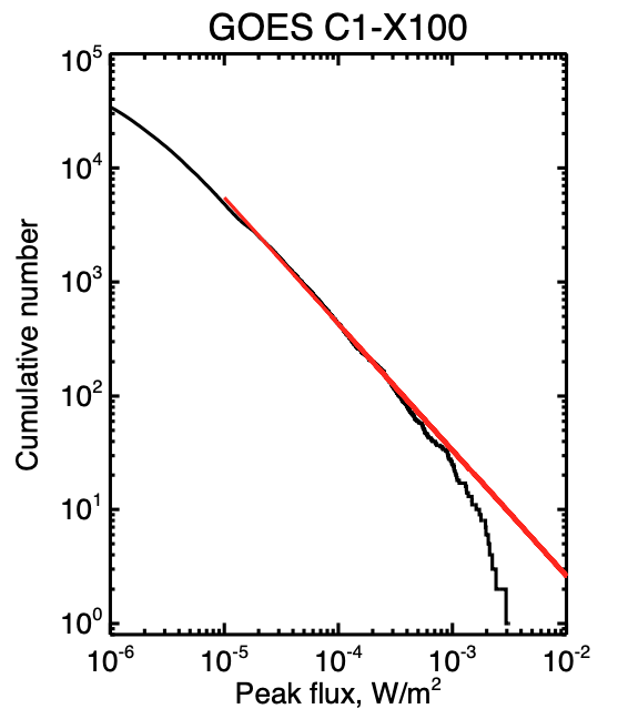
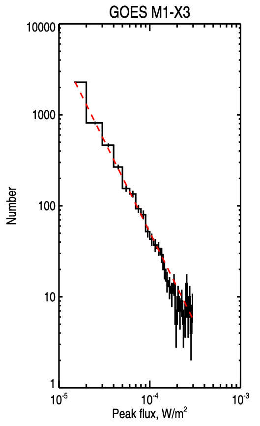
Figure 5.: Left, downward-cumulative distribution of 47,173 GOES soft X-ray flares (C1 and above) over 1975–2022, in bins of $10^{-7}$ W/m² (B1) width. Right, differential distribution fitted over the range M1–X3 only, with a red line showing a least-squares fit to the M1-X3 range. The (extrapolated) red line in the left panel comes from the same fit. fig:cumulative

The cumulative distribution contains 6,344 events above a background-subtracted peak flux 10^-5 W/m² (M1) and has a power-law appearance at the lowest range. We fit the range up to the equivalent X3 flux as shown in Table tab:fits, using the maximum-likelihood method (e.g., Crawford, Jauncey, and Murdoch, 1970; D’Huys et al., 2016). The binned distribution (Figure fig:cumulative, right panel) shows a consistent fit, slightly steeper as expected, and we adopt its uncertainty value for extrapolations. The slope is constent with 2.0 but without background subtraction this would not be the case; the slope of the power-law range of the ODF is significantly steeper in this case.

Table 4.: Power-law $\alpha$ (differential) over equivalent M1-X3 rangetab:fits

Maximum Likelihood	$1.973\pm 0.014$	Backgrounds subtracted
Maximum Likelihood	$2.148\pm 0.015$	Backgrounds not subtracted
Binned	2.008 $\pm\ 0.048$	Backgrounds subtracted
Binned	2.172 $\pm\ 0.043$	Backgrounds not subtracted

The ODF shown in Figure fig:cumulative (left panel) shows a deficit of major events, and because the GOES database has essentially complete sampling over its 46 years to time of writing, we can now discuss its implications. We have no theoretical guidance for any particular form for the rollover and do not attempt here to characterize it with an empirical formula, such as a power law with an exponential cutoff or the alternative of a broken power law (e.g., Band et al., 1993), which would have distinctly different predictions for longer time scales. Instead we just characterize the significance of the rollover by extrapolating the observed power law from the weaker events (below X3), with $\alpha=1.973$, as described in Table tab:numbers (left columns). The distributions (observed and predicted, based on the results in Table tab:fits) clearly disagree strongly, with the simple power law significantly overestimating the event numbers in the observable range. The inclusion of the historical Carrington event itself (e.g., Cliver and Dietrich, 2013; Hudson, 2021) could not alter this conclusion significantly based on the equivalent GOES class inferred from proxy data in these papers. Clarke et al. (2010) do suggest a value of about X42 (old scale, without the factor 1.43) based on this flare’s geomagnetic effect (Stewart, 1861). Recently Hayakawa et al. (2023) also suggested X56 (old scale) based on re-analysis of the original optical sighting. We note the similarity of the radio-burst ODF discussed by Nita et al. (2002), who also found a paucity of great events (noting as well the possibility of a contribution by instrumental saturation).

Table 5.: Event numbers normalized at X1tab:numbers

Class	Observation	Expected number	Predicted number	Gopalswamy (2018)
		(M1-X3 power law)	(this work)	(power law $\alpha=2.31$)
X1	609	609	609	609
X3	174	208	169	47
X10	37	64	35	2
X30	4	22	5	0
X100	0	14	0	0
X300	0		0	0

4 Fitting the CCDF: the “superflares”

sec:extrapolation

The complete sample now lets us fit empirical functions to the GOES complementary cumulative occurrence distribution function (CCDF). By doing this we can have a mathematical basis for extending to still greater events than have been observed, such as the SXR flares inferred for the cosmogenic (radioisotope-based) solar energetic proton (SEP) events (Miyake et al., 2012; Usoskin et al., 2013), with others now noted discovered or identified across the time scale of the Holocene (Cliver et al., 2022; Usoskin, 2023). Superflares observed on other stars are arbitrarily defined as those with bolometric energy $>10^{33}$ erg (Schaefer, King, and Deliyannis, 2000). In comparison, the largest flares directly observed on the Sun have radiative energies of at most $\approx 4\times 10^{32}$  erg (e.g., Emslie et al., 2012). The departure of the observed occurrence distribution (the ODF) from a simple power law complicates this extension, which must now have additional parameters to describe the observed roll-over, just where small numbers lead to uncertain statistics. We attack this problem by fitting the empirical CCDF to one of the mathematical forms used by Sakurai (2022) who tested four different fits: a simple power law (one free parameter), tapered power law (two), gamma function (two), and Weibull (two). As noted by Sakurai, the Weibull distribution does not fit the roll-over (required by the lack of extreme events) as well as the other two-parameter fits, and for simplicity we use only the tapered power law here:

$$\ilabel{eq:ccdfpwrexp}CCDF=A(S/S_{0})^{-\alpha-1}e^{-\beta(S-S_{0})/S_{0}}\ ,$$ (2)

representing the CCDF of $S$ (here in W/m²) above a threshold peak flux S${}_{0}=10^{-4}$ W/m² (the X1 level). Note that this (or any other) functional form for the CCDF is purely a mathematical convenience since we have no particular physical motivation for any of the options. We wish to estimate the uncertainties the CCDF fit function over the observed range. Possible goodness-of-fit approaches include $\chi^{2}$ and Kolmogorov-Smirnov tests (Sakurai, 2022) for the entire distribution, but we choose instead simply to freeze the $\alpha$ parameter at Sakurai’s value, which agrees with our maximum-likelihood fit to the M3–X10 range as described in Section 3.2. This means that our estimated uncertainties depend only on the statistics of the roll-over region itself, namely the X10-class events. We estimate uncertainties on the $\beta$ parameter by assuming a Poisson distribution for events at X10 class or above, for which we find a total of 37$\pm$6 events, leading to parameters $[\alpha,\beta]=[0.973,0.0336^{+0.011,-0.021}]$. Figure fig:prediction_final shows the results in terms of the CCDF and the waiting time vs. GOES peak flux. This can be crudely transformed into total event energy $E$ by using Eq. 5 of Cliver et al. (2022), $E=3.3\times 10^{31}(S/S_{X1})^{0.72}$ erg as scaled to the GOES peak flux $S$ in units of $10^{-4}$ W/m². The upper limit for the total energy of a solar flare on the Holocene time scale of about 10⁴ years thus becomes $\approx$10³³ erg.

We note that CCDF extrapolations by Gopalswamy (2018) and by Sakurai (2022), based on samples of unscreened GOES flares with no correction for the saturated (clipped) events, obtained similar results. Using a Weibull function fit, Gopalswamy (2018) obtained 100-yr and 1000-yr estimates of X63 and X144, respectively (with the 1.43 correction applied) while Sakurai (2022) estimated that a once-per-1000-yr flare would have a X100 GOES class. Table tab:numbers also shows an alternative power-law extrapolation to extreme values (Gopalswamy 2018, Fig. 5), along with our tapered power law, in the right two columns. These values compare with the our nominal 100-yr (X75) and 1000-yr (X110) estimates in Table tab:return. All of these estimates fall short of the (current scaling) $\approx$X$400\pm 200$ ($\approx 2\times 10^{33}$ erg) estimate obtained by (Cliver et al., 2020, cf. Cliver et al. 2022) for the cosmogenic-nuclide-based solar energetic particle (SEP) event of 774 AD with an inferred $>$200 MeV fluence 80$\times$ larger than the largest SEP event of the modern era, that associated with the flare SOL1956-02-23 (Koldobskiy et al., 2021, 2023).

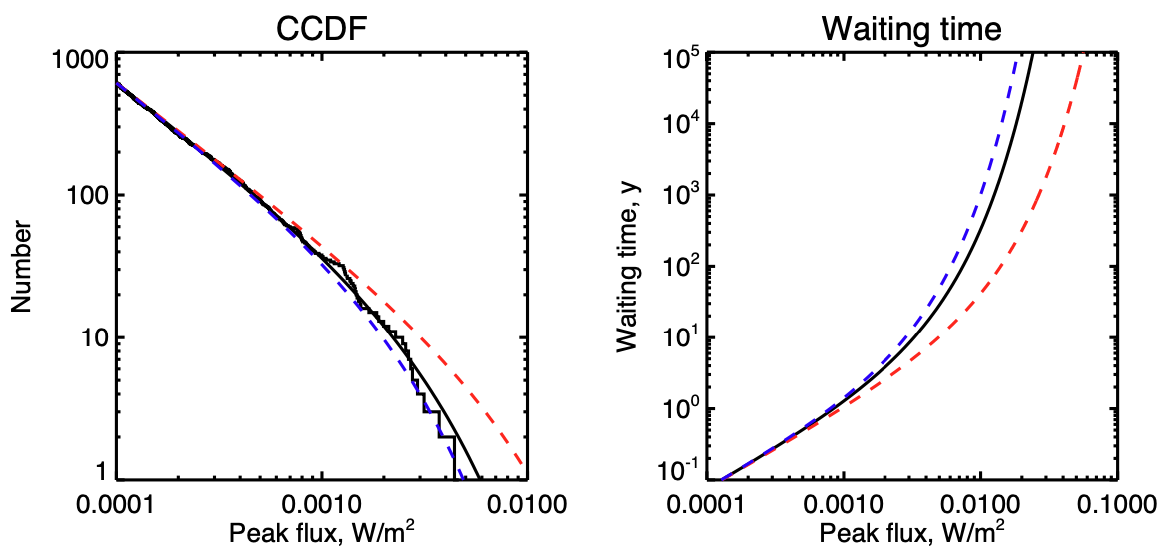
Figure 6.: Left, downward-cumulative distribution of 609 GOES soft X-ray flares (new X1 level and above) over 1975–2022. Right, the same information inverted to waiting time for a flare at a given GOES class. See text for details. fig:prediction˙final

From the CCDF in Figure fig:prediction_final (left), we can determine the GOES event occurrence on 10-, 100-, and 10,000-yr time scales from the corresponding waiting-time plot on the right of the figure, which we interpet in Table tab:return.

Table 6.: Probable event magnitudes for long time scalestab:return

	GOES class	Bolometric Energy∗
		($10^{32}$ erg)
100-yr	X60-X75-X115	4.9-5.7-7.8
1000-yr	X100-X110-X260	7.0-7.5-14.0
104-yr	X140-X180-X400	7.8-10.7-19.1

^∗Based on the Kretzschmar-Schrijver relationship between
GOES class and bolometric energy, Eq. 5 in Cliver et al. (2022),
with the adjustment for the new GOES as described
in Section 8.2.1 therein.

5 Conclusions

sec:conclusions

In this analysis of GOES SXR events from 1975-2022, we have estimated the peak fluxes for 12 1-8 Å events of class $\geq$X10 that saturated (or more accurately were clipped) prior to reaching their maximum. We did so by developing a technique of extrapolating the clipped time profile across the saturation gap by two independent methods that we verified on a set of 10 $\geq$X10 non-saturated events. In addition, we applied a significant calibration correction (43% increase in 1-8 Å peak fluxes) to the GOES-1 through GOES-15 data (1975-2016) and also subtracted an event-by-event background for all flares with GOES class $\geq$C1. For events below the saturation range, we fitted the ODF with a power-law with index near 2.0, consistent with the results of Aschwanden and Freeland (2012) We have now included the saturated events by a uniform treatment of their extrapolated time profiles, as verified on a set of non-saturating events. The observed ODF departs from its power-law character at the high end; extrapolation to higher GOES fluxes beyond the $\approx$X10-level over-predicts the observed occurrence frequency of such events.

Extrapolation of a tapered-power-law fit to the GOES 1-8 Å CCDF yields a nominal (revised SWPC scaling) 100-yr event of X75, comparable to a recent $\approx$X80 assessment of the Carrington event (Hayakawa et al., 2023), and a 1000-yr event of X110, bracketed by recent (new-scale) estimates of X100 (Sakurai, 2022) and X144 (Gopalswamy, 2018) based on GOES event samples without event-screening, back-ground subtraction, or saturation correction. The agreement of these various studies suggests a certain robustness for such estimates. Our nominal 1000-yr estimate of X180 (X140-X400), however, falls outside the estimate of X400$\pm$200 peak GOES flux (Cliver et al., 2020, 2022) for the flare associated with the huge cosmogenic-nuclide-based SEP event of 774 CE (Koldobskiy et al., 2021, 2023), although the uncertainties overlap. We note that such comparisons involve a complicated chain of inference (solar event $\rightarrow$ soft X-rays $\rightarrow$ CME $\rightarrow$ SEPs $\rightarrow$ Earth impact $\rightarrow$ radioisotope record), each step of which involves assumptions.

Acknowledgments

The authors have benefited from participation at several ISSI Team meetings. This comprehensive study would not have been possible without the careful work of our late friend and colleague, Richard Schwartz.

Appendix: The X10-class GOES events, revisedsec:appendix

Table tab:original provides new GOES peak-flux estimates for 23 X10-class events (original listing) in the database, and Table tab:augmentation extends it to a total of 38 according to the correction factor of 1.43 applied to the 1-8 Å magnitudes. The sorting here is by our new estimates; note that only event No. 19 (X9.3) did not have an original GOES class at $\geq$X10 (though GOES-15 and GOES-16 differed on this point). The new magnitudes adjust peak flux estimates from GOES-12 through GOES-15 and earlier to match the calibrations of the GOES-R series.

The listed peak fluxes do not exactly correspond to the older class ratings, based on 1-minute sampling, but correspond almost exactly at two significant figures: our top entry of 45.9$\times 10^{-3}$ W/m² can be taken as X46 (or X32 on the old scale). We note that the background corrections, though important in characterizing the ODF, normally do not matter for the greatest events. These tables are in order of our new estimation of GOES peak flux levels, incorporating the event-by-event background correction, and using the full time resolution of the sampling rather than 1-min integrations. According to our validation procedure for the corrections to the saturated events (Section sec:uncertainties) we believe that the individual events have peak fluxes estimated with an rms precision of about 3%, which is small compared with the nominal XRS radiometric error (see Figure fig:rats_plot), which we have estimated at 20%. SOL1978-07-11T10:58 has a compromised calibration since GOES-2 did not have sufficient overlapping in-orbit data from other GOES instruments. Most likely the GOES peak flux for SOL2003-11-04 is a lower limit, since the flare was a limb event and somewhat occulted, so this event is probably the greatest GOES event in our database.

Table 7.: The greatest GOES events (original)tab:original

Rank	IAU Identifier	Old class	Satellite	Saturated?	Peak Flux
				Y/N	10-3 W/m2
1	SOL1978-07-11T10:58	X15.0	GOES2	Y	X45.9
2	SOL2003-11-04T19:50	X28.0	GOES10	Y	X43.2
3	SOL1991-06-15T08:31	X12.0	GOES6	Y	X34.7
4	SOL1991-06-04T03:47	X12.0	GOES6	Y	X32.0
5	SOL1991-06-06T01:12	X12.0	GOES6	Y	X30.2
6	SOL2001-04-02T21:51	X20.0	GOES8	Y	X29.6
7	SOL1991-06-01T15:29	X12.0	GOES6	Y	X28.3
8	SOL1989-08-16T01:17	X20.0	GOES6	Y	X28.0
9	SOL2003-10-28T11:10	X17.2	GOES10	N	X25.7
10	SOL2005-09-07T17:40	X17.0	GOES12	N	X24.6
11	SOL1989-10-19T12:55	X13.0	GOES6	Y	X23.1
12	SOL2001-04-15T13:50	X14.4	GOES8	N	X21.1
13	SOL1984-04-24T24:01	X13.0	GOES5	Y	X19.7
14	SOL1989-03-06T14:10	X15.0	GOES6	Y	X19.3
15	SOL1982-12-15T01:59	X12.9	GOES2	N	X19.0
16	SOL1991-06-11T02:29	X12.0	GOES6	Y	X17.0
17	SOL1991-01-25T06:30	X10.0	GOES6	N	X15.7
18	SOL2003-10-29T20:49	X10.0	GOES10	N	X15.5
19	SOL1991-06-09T01:40	X10.0	GOES6	N	X15.1
20	SOL1984-05-20T22:41	X10.1	GOES5	N	X14.8
21	SOL2017-09-06T12:02	X9.3	GOES16	N	X14.8
22	SOL1982-06-06T16:54	X12.0	GOES2	N	X14.7
23	SOL1982-12-17T18:58	X10.1	GOES2	N	X14.7

^∗The GOES calibration for this early event is relatively weak; see Figure fig:rats_plot

Table 8.: The greatest GOES events (augmentation)tab:augmentation

Rank	IAU Identifier	Old class	Satellite	Peak flux
				10-3 W/m2
24	SOL1989-09-29T11:33	X9.80	GOES6	X14.2
25	SOL1990-05-24T20:49	X9.30	GOES6	X14.1
26	SOL1991-03-22T22:45	X9.40	GOES6	X13.8
27	SOL2003-11-02T17:25	X8.30	GOES10	X13.3
28	SOL1997-11-06T11:55	X9.40	GOES8	X13.1
29	SOL2006-12-05T10:35	X9.00	GOES12	X13.1
30	SOL2017-09-10T16:06	X8.2	GOES16	X13.0
31	SOL1992-11-02T03:08	X9.00	GOES6	X13.0
32	SOL1980-11-06T03:48	X9.00	GOES2	X12.8
33	SOL1982-06-03T11:48	X8.00	GOES2	X11.8
34	SOL1989-10-24T18:31	X5.70	GOES6	X11.5
35	SOL2011-08-09T08:05	X6.90	GOES15	X10.7
36	SOL1991-03-04T14:03	X7.10	GOES6	X10.4
37	SOL2005-01-20T07:01	X7.10	GOES12	X10.2
38	SOL1982-07-12T09:18	X7.10	GOES2	X10.1

References

- Akabane (1956) Akabane, K.: 1956, Some Features of Solar Radio Bursts at Around 3000 Mc/s. PASJ 8, 173. ADS.
- Aschwanden and Freeland (2012) Aschwanden, M.J., Freeland, S.L.: 2012, Automated Solar Flare Statistics in Soft X-Rays over 37 Years of GOES Observations: The Invariance of Self-organized Criticality during Three Solar Cycles. ApJ 754, 112. DOI. ADS.
- Band et al. (1993) Band, D., Matteson, J., Ford, L., Schaefer, B., Palmer, D., Teegarden, B., Cline, T., Briggs, M., Paciesas, W., Pendleton, G., Fishman, G., Kouveliotou, C., Meegan, C., Wilson, R., Lestrade, P.: 1993, BATSE observations of gamma-ray burst spectra. I - Spectral diversity. ApJ 413, 281. DOI. ADS.
- Bornmann (1990) Bornmann, P.L.: 1990, Limits to derived flare properties using estimates for the background fluxes - Examples from GOES. ApJ 356, 733. DOI. ADS.
- Cannon (2013) Cannon, P.S.: 2013, Extreme Space Weather—A Report Published by the UK Royal Academy of Engineering. Space Weather 11, 138. DOI. ADS.
- Chamberlin et al. (2009) Chamberlin, P.C., Woods, T.N., Eparvier, F.G., Jones, A.R.: 2009, Next generation x-ray sensor (XRS) for the NOAA GOES-R satellite series. In: Society of Photo-Optical Instrumentation Engineers (SPIE) Conference Series, Society of Photo-Optical Instrumentation Engineers (SPIE) Conference Series 7438. DOI. ADS.
- Clarke et al. (2010) Clarke, E., Rodger, C., Clilverd, M., Humphries, T., Baillie, O., Thomson, A.: 2010, An estimation of the Carrington flare magnitude from solar flare effects (sfe) in the geomagnetic records (UK NAM, unpublished).
- Cliver and Dietrich (2013) Cliver, E.W., Dietrich, W.F.: 2013, The 1859 space weather event revisited: limits of extreme activity. Journal of Space Weather and Space Climate 3, A260000. DOI. ADS.
- Cliver et al. (2020) Cliver, E.W., Hayakawa, H., Love, J.J., Neidig, D.F.: 2020, On the Size of the Flare Associated with the Solar Proton Event in 774 AD. ApJ 903, 41. DOI. ADS.
- Cliver et al. (2022) Cliver, E.W., Schrijver, C.J., Shibata, K., Usoskin, I.G.: 2022, Extreme solar events. Living Reviews in Solar Physics 19, 2. DOI. ADS.
- Crawford, Jauncey, and Murdoch (1970) Crawford, D.F., Jauncey, D.L., Murdoch, H.S.: 1970, Maximum-Likelihood Estimation of the Slope from Number-Flux Counts of Radio Sources. ApJ 162, 405. DOI. ADS.
- D’Huys et al. (2016) D’Huys, E., Berghmans, D., Seaton, D.B., Poedts, S.: 2016, The Effect of Limited Sample Sizes on the Accuracy of the Estimated Scaling Parameter for Power-Law-Distributed Solar Data. Sol. Phys. 291, 1561. DOI. ADS.
- Emslie et al. (2012) Emslie, A.G., Dennis, B.R., Shih, A.Y., Chamberlin, P.C., Mewaldt, R.A., Moore, C.S., Share, G.H., Vourlidas, A., Welsch, B.T.: 2012, Global Energetics of Thirty-eight Large Solar Eruptive Events. ApJ 759, 71. DOI. ADS.
- Feldman, Doschek, and Klimchuk (1997) Feldman, U., Doschek, G.A., Klimchuk, J.A.: 1997, The Occurrence Rate of Soft X-Ray Flares as a Function of Solar Activity. ApJ 474, 511. DOI. ADS.
- Freeland and Handy (1998) Freeland, S.L., Handy, B.N.: 1998, Data Analysis with the SolarSoft System. Sol. Phys. 182, 497. DOI. ADS.
- Garcia (1994) Garcia, H.A.: 1994, Temperature and emission measure from GOES soft X-ray measurements. Sol. Phys. 154, 275. DOI. ADS.
- Gopalswamy (2018) Gopalswamy, N.: 2018, Chapter 2 - Extreme Solar Eruptions and their Space Weather Consequences. In: Buzulukova, N. (ed.) Extreme Events in Geospace, Elsevier, 37. ISBN 978-0-12-812700-1. DOI. https://www.sciencedirect.com/science/article/pii/B9780128127001000029.
- Gopalswamy et al. (2005) Gopalswamy, N., Barbieri, L., Cliver, E.W., Lu, G., Plunkett, S.P., Skoug, R.M.: 2005, Introduction to violent Sun-Earth connection events of October-November 2003. Journal of Geophysical Research (Space Physics) 110, A09S00. DOI. ADS.
- Hanser and Sellers (1996) Hanser, F.A., Sellers, F.B.: 1996, Design and calibration of the GOES-8 solar x-ray sensor: the XRS. In: Washwell, E.R. (ed.) GOES-8 and Beyond, Proc. S.P.I.E. 2812, 344. DOI. ADS.
- Hapgood et al. (2021) Hapgood, M., Angling, M.J., Attrill, G., Bisi, M., Cannon, P.S., Dyer, C., Eastwood, J.P., Elvidge, S., Gibbs, M., Harrison, R.A., Hord, C., Horne, R.B., Jackson, D.R., Jones, B., Machin, S., Mitchell, C.N., Preston, J., Rees, J., Rogers, N.C., Routledge, G., Ryden, K., Tanner, R., Thomson, A.W.P., Wild, J.A., Willis, M.: 2021, Development of Space Weather Reasonable Worst Case Scenarios for the UK National Risk Assessment. Space Weather 19, e02593. DOI. ADS.
- Hayakawa et al. (2023) Hayakawa, H., Bechet, S., Clette, F., Hudson, H.S., Maehara, H., Namekata, K., Notsu, Y.: 2023, Magnitude Estimates for the Carrington Flare in 1859 September: As Seen from the Original Records. ApJ 954, L3. DOI. ADS.
- Hock (2012) Hock, R.A.: 2012, The Role of Solar Flares in the Variability of the Extreme Ultraviolet Solar Spectral Irradiance. PhD thesis, University of Colorado at Boulder. ADS.
- Hudson (1991) Hudson, H.S.: 1991, Solar flares, microflares, nanoflares, and coronal heating. Sol. Phys. 133, 357. DOI. ADS.
- Hudson (2021) Hudson, H.S.: 2021, Carrington Events. ARA&A 59. DOI. ADS.
- Kahler and Kreplin (1991) Kahler, S.W., Kreplin, R.W.: 1991, The NRL SOLRAD X-ray detectors: A summary of the observations and a comparison with the SMS/GOES detectors. Sol. Phys. 133, 371. DOI. ADS.
- Kiplinger and Garcia (2004) Kiplinger, A.L., Garcia, H.A.: 2004, Soft X-ray Parameters of the Great Flares of Active Region 486. In: American Astronomical Society Meeting Abstracts #204, Bulletin of the American Astronomical Society 36, 739. ADS.
- Koldobskiy et al. (2021) Koldobskiy, S., Raukunen, O., Vainio, R., Kovaltsov, G.A., Usoskin, I.: 2021, New reconstruction of event-integrated spectra (spectral fluences) for major solar energetic particle events. A&A 647, A132. DOI. ADS.
- Koldobskiy et al. (2023) Koldobskiy, S., Mekhaldi, F., Kovaltsov, G., Usoskin, I.: 2023, Multiproxy Reconstructions of Integral Energy Spectra for Extreme Solar Particle Events of 7176 BCE, 660 BCE, 775 CE, and 994 CE. Journal of Geophysical Research (Space Physics) 128, e2022JA031186. DOI. ADS.
- Kretzschmar (2011) Kretzschmar, M.: 2011, The Sun as a star: observations of white-light flares. A&A 530, A84. DOI. ADS.
- Machol et al. (2020) Machol, J.L., Eparvier, F.G., Viereck, R.A., Woodraska, D.L., Snow, M., Thiemann, E., Woods, T.N., McClintock, W.E., Mueller, S., Eden, T.D., Meisner, R., Codrescu, S., Bouwer, S.D., Reinard, A.A.: 2020, Chapter 19 - GOES-R Series Solar X-ray and Ultraviolet Irradiance. In: Goodman, S.J., Schmit, T.J., Daniels, J., Redmon, R.J. (eds.) The GOES-R Series, Elsevier, 233 . ISBN 978-0-12-814327-8. DOI. http://www.sciencedirect.com/science/article/pii/B9780128143278000196.
- Machol et al. (2022) Machol, J., Viereck, R., Peck, C., Mothersbaugh III, J.: 2022, GOES XRS OPERATIONAL DATA (NOAA). Technical report.
- Miyake et al. (2012) Miyake, F., Nagaya, K., Masuda, K., Nakamura, T.: 2012, A signature of cosmic-ray increase in AD 774-775 from tree rings in Japan. Nature 486, 240. DOI. ADS.
- Moore, Chamberlin, and Hock (2014) Moore, C.S., Chamberlin, P.C., Hock, R.: 2014, Measurements and Modeling of Total Solar Irradiance in X-class Solar Flares. ApJ 787, 32. DOI. ADS.
- Neupert (2011) Neupert, W.M.: 2011, Intercalibration of Solar Soft X-Ray Broad Band Measurements from SOLRAD 9 through GOES-12. Sol. Phys. 272, 319. DOI. ADS.
- Nita et al. (2002) Nita, G.M., Gary, D.E., Lanzerotti, L.J., Thomson, D.J.: 2002, The Peak Flux Distribution of Solar Radio Bursts. ApJ 570, 423. DOI. ADS.
- Plutino et al. (2023) Plutino, N., Berrilli, F., Del Moro, D., Giovannelli, L.: 2023, A new catalogue of solar flare events from soft X-ray GOES signal in the period 1986-2020. Advances in Space Research 71, 2048. DOI. ADS.
- Ryan et al. (2012) Ryan, D.F., Milligan, R.O., Gallagher, P.T., Dennis, B.R., Tolbert, A.K., Schwartz, R.A., Young, C.A.: 2012, The Thermal Properties of Solar Flares over Three Solar Cycles Using GOES X-Ray Observations. The Astrophysical Journal Supplement Series 202, 11. DOI. ADS.
- Sakurai (2022) Sakurai, T.: 2022, Probability Distribution Functions of Solar and Stellar Flares. Physics 5, 11. DOI. ADS.
- Schaefer, King, and Deliyannis (2000) Schaefer, B.E., King, J.R., Deliyannis, C.P.: 2000, Superflares on Ordinary Solar-Type Stars. ApJ 529, 1026. DOI. ADS.
- Stewart (1861) Stewart, B.: 1861, On the Great Magnetic Disturbance Which Extended from August 28 to September 7, 1859, as Recorded by Photography at the Kew Observatory. Philosophical Transactions of the Royal Society of London Series I 151, 423. ADS.
- Swalwell et al. (2018) Swalwell, B., Dalla, S., Kahler, S., White, S.M., Ling, A., Viereck, R., Veronig, A.: 2018, The Reported Durations of GOES Soft X-Ray Flares in Different Solar Cycles. Space Weather 16, 660. DOI. ADS.
- Thomas, Starr, and Crannell (1985) Thomas, R.J., Starr, R., Crannell, C.J.: 1985, Expressions to Determine Temperatures and Emission Measures for Solar X-Ray Events from Goes Measurements. Sol. Phys. 95, 323. DOI. ADS.
- Thomson, Rodger, and Clilverd (2005) Thomson, N.R., Rodger, C.J., Clilverd, M.A.: 2005, Large solar flares and their ionospheric D region enhancements. Journal of Geophysical Research (Space Physics) 110, A06306. DOI. ADS.
- Usoskin (2023) Usoskin, I.G.: 2023, A history of solar activity over millennia. Living Reviews in Solar Physics 20, 2. DOI. ADS.
- Usoskin et al. (2013) Usoskin, I.G., Kromer, B., Ludlow, F., Beer, J., Friedrich, M., Kovaltsov, G.A., Solanki, S.K., Wacker, L.: 2013, The AD775 cosmic event revisited: the Sun is to blame. A&A 552, L3. DOI. ADS.
- Veronig et al. (2002) Veronig, A., Temmer, M., Hanslmeier, A., Otruba, W., Messerotti, M.: 2002, Temporal aspects and frequency distributions of solar soft X-ray flares. A&A 382, 1070. DOI. ADS.
- Wende (1972) Wende, C.D.: 1972, The Normalization of Solar X-Ray Data from Many Experiments. Sol. Phys. 22, 492. DOI. ADS.
- White, Thomas, and Schwartz (2005) White, S.M., Thomas, R.J., Schwartz, R.A.: 2005, Updated Expressions for Determining Temperatures and Emission Measures from Goes Soft X-Ray Measurements. Sol. Phys. 227, 231. DOI. ADS.
- Woods, Kopp, and Chamberlin (2006) Woods, T.N., Kopp, G., Chamberlin, P.C.: 2006, Contributions of the solar ultraviolet irradiance to the total solar irradiance during large flares. Journal of Geophysical Research (Space Physics) 111, A10S14. DOI. ADS.
- Woods et al. (2012) Woods, T.N., Eparvier, F.G., Hock, R., Jones, A.R., Woodraska, D., Judge, D., Didkovsky, L., Lean, J., Mariska, J., Warren, H., McMullin, D., Chamberlin, P., Berthiaume, G., Bailey, S., Fuller-Rowell, T., Sojka, J., Tobiska, W.K., Viereck, R.: 2012, Extreme Ultraviolet Variability Experiment (EVE) on the Solar Dynamics Observatory (SDO): Overview of Science Objectives, Instrument Design, Data Products, and Model Developments. Sol. Phys. 275, 115. DOI. ADS.