Enhancing Group Fairness in Online Settings Using Oblique Decision Forests

Abstract

Fairness, especially group fairness, is an important consideration in the context of machine learning systems. The most commonly adopted group fairness-enhancing techniques are in-processing methods that rely on a mixture of a fairness objective (e.g., demographic parity) and a task-specific objective (e.g., cross-entropy) during the training process. However, when data arrives in an online fashion – one instance at a time – optimizing such fairness objectives poses several challenges. In particular, group fairness objectives are defined using expectations of predictions across different demographic groups. In the online setting, where the algorithm has access to a single instance at a time, estimating the group fairness objective requires additional storage and significantly more computation (e.g., forward/backward passes) than the task-specific objective at every time step. In this paper, we propose Aranyani, an ensemble of oblique decision trees, to make fair decisions in online settings. The hierarchical tree structure of Aranyani enables parameter isolation and allows us to efficiently compute the fairness gradients using aggregate statistics of previous decisions, eliminating the need for additional storage and forward/backward passes. We also present an efficient framework to train Aranyani and theoretically analyze several of its properties. We conduct empirical evaluations on 5 publicly available benchmarks (including vision and language datasets) to show that Aranyani achieves a better accuracy-fairness trade-off compared to baseline approaches.

1 Introduction

Critical applications of machine learning, such as hiring (Dastin, 2022) and criminal recidivism (Larson et al., 2016), require special attention to avoid perpetuating biases present in training data (Corbett-Davies et al., 2017; Buolamwini & Gebru, 2018; Raji & Buolamwini, 2019). Group fairness, which is a well-studied paradigm for mitigating such biases in machine learning (Mehrabi et al., 2021; Hort et al., 2022), tries to achieve statistical parity of a system’s predictions among different demographic (or protected) groups (e.g., gender or race). In general, group fairness-enhancing techniques can be broadly categorized into three categories: pre-processing (Zemel et al., 2013; Calmon et al., 2017), post-processing (Hardt et al., 2016; Pleiss et al., 2017; Alghamdi et al., 2022), and in-processing (Quadrianto & Sharmanska, 2017; Agarwal et al., 2018; Lowy et al., 2022) techniques. Most of these approaches rely on group fairness objectives that are optimized alongside task-specific objectives in an offline setting (Dwork et al., 2012). Group fairness objectives (e.g., demographic parity) are defined using expectations of predictions across different demographic groups, which requires the system to have access to labeled data from different groups. However, in many modern applications (e.g., moderation decisions for social media content), data arrives in an online fashion – one instance at a time, and ML systems need to be continuously updated using the data stream.

In the online setting, optimizing for group fairness poses several unique challenges. Central to this paper, in-processing techniques require additional storage or computation since the system only has access to a single input instance at any given time. In online settings, naively training the model using group fairness loss involves storing all (or at least a subset of) the input instances seen so far, and performing forward/backward passes through the model using these instances at each step of online learning, which can be computationally expensive. We also note that other techniques such as pre-processing techniques are clearly impractical as they require prior access to data. Post-processing techniques typically assume black-box access to a trained model and a held-out validation set (Hardt et al., 2016), which can be impractical or expensive to acquire during online learning.

In this paper, we present a novel framework Aranyani, which consists of an ensemble of oblique decision trees. Aranyani uses the structural properties of the tree to enhance group fairness in decisions made during online learning. The final prediction in oblique trees is a combination of local decisions at individual tree nodes. We show that imposing group fairness constraints on local node-level decisions results in parameter isolation, which empirically leads to better and fairer solutions. In the online setting, we show that maintaining the aggregate statistics of the local node-level decisions allows us to efficiently estimate group fairness gradients, eliminating the need for additional storage or forward/backward passes. We present an efficient framework to train Aranyani using state-of-the-art autograd libraries and modern accelerators. We also theoretically study several properties of Aranyani including the convergence of gradient estimates. Empirically, we observe that Aranyani achieves the best accuracy-fairness trade-off on 5 different online learning setups.

Our paper is organized as follows: (a) We begin by introducing the fundamentals of oblique decision trees and provide the details of oblique decision forests used in Aranyani (Section 2), (b) We describe the problem setup and discuss how to enforce group fairness in the simpler offline setting (Section 3.1 & 3.2), (c) We describe the functioning of Aranyani in the online setting (Section 3.3), (d) We describe an efficient training procedure for oblique decision forests that enables gradient computation using back-propagation (Section 3.4), (e) We theoretically analyze several properties of Aranyani (Section 4), and (f) We describe the experimental setup and results of Aranyani and other baseline approaches on several datasets (Section 5). We observe that Aranyani achieves the best accuracy-fairness tradeoff, and provides significant time and memory complexity gains compared to naively storing input instances to compute the group fairness loss.

2 Oblique Decision Trees

We introduce our proposed framework, Aranyani, an ensemble of oblique decision trees, for achieving group fairness in an online setting. In this section, we introduce the fundamentals of oblique decision trees and discuss the details of the prediction function used in Aranyani. Similar to a conventional decision tree, an oblique decision tree splits the input space to make predictions by routing samples through different paths along the tree. However, unlike a decision tree, which only makes axis-aligned splits, an oblique decision tree can make arbitrary oblique splits by using routing functions that consider all input features. The routing functions in oblique decision tree nodes can be parameterized using neural networks (Murthy et al., 1994; Jordan & Jacobs, 1994). This allows it to potentially fit arbitrary boundary structures more effectively. We formally describe the details of the oblique decision tree structure below:

Definition 1 (Oblique binary decision tree (Karthikeyan et al., 2022)).

An oblique tree of height $h$ represents a function $f(\mathbf{x;W,B,\Theta}):\mathbb{R}^{d}\rightarrow\mathbb{R}^{c}$ parameterized by $\mathbf{w}_{ij}\in\mathbb{R}^{d}$, $\mathbf{b}_{ij}\in\mathbb{R}$ at $(i,j)$-th node ($j$-th node at depth $i$). Each node computes $n_{ij}(\mathbf{x})=\mathbf{w}_{ij}^{T}\mathbf{x}+\mathbf{b}_{ij}>0$, which decides whether $\mathbf{x}$ must traverse the left or right child. After traversing the tree, input $\mathbf{x}$ arrives at the $l$-th leaf that outputs $\theta_{l}\in\mathbb{R}^{c}$ ($c>1$ for classification and $c=1$ for regression).

The oblique tree parameters $(\mathbf{W},\mathbf{B},\mathbf{\Theta})$ can be learned using gradient descent (Karthikeyan et al., 2022). However, the hard routing in oblique decision trees ($\mathbf{x}$ is routed either to the left or right child) makes the learning process non-trivial. In our work, we consider a modified soft version of oblique trees where an input $\mathbf{x}$ is routed to both left and right child at every tree node with certain probabilities based on the node output, $n_{ij}(\mathbf{x})$.

Definition 2 (Soft-Routed Oblique binary decision tree).

Using the same parameterization in Definition 1, soft-routed oblique trees route $\mathbf{x}$ to both children at each node with a certain probability. At $(i,j)$-th node, the probability that $\mathbf{x}$ is routed to the left node $p(\swarrow)=n_{ij}(\mathbf{x})$, and the right node is $p(\searrow)=1-n_{ij}(\mathbf{x})$, where $n_{ij}(\mathbf{x})=g(\mathbf{w}_{ij}^{T}\mathbf{x}+\mathbf{b}_{ij})$ and $g(x)\in[0,1]$ is an activation function. The output $f(\mathbf{x})=\sum_{l}p_{l}(\mathbf{x})\theta_{l}$, where $p_{l}(\mathbf{x})$ is the probability with which $\mathbf{x}$ reaches the $l$-th leaf.

In soft-routed oblique decision trees, we observe that the prediction $f(\mathbf{x})$ is a linear combination of all the leaf parameters. The coefficients $p_{l}(\mathbf{x})=\prod_{i=1}^{h}n_{i,A(i,l)}(\mathbf{x})$ is the product of all probabilities along the path from the root to the $l$-th leaf and $A(i,l)$ is the $l$-th leaf’s ancestor at depth $i$. We observe that learning the parameters of the soft-routed tree structure is much easier as we can easily compute the gradients of parameters w.r.t. $f(\mathbf{x})$ using backpropagation. We further improve the efficiency by computing $f(\mathbf{x})$ using matrix operations as described in Section 3.4. In our work, we use a complete binary tree of height $h$ to parameterize obliques trees. Note that the proposed soft-routed oblique trees are reminiscent of the sigmoid tree decomposition (Yang et al., 2019) used in alleviating the softmax bottleneck.

We use an ensemble of trees and the expected output as the final prediction to reduce the variance and increase the predictive power of the outputs of soft-routed oblique decision trees. We call this soft-routed oblique forest, which is computed as: $f(\mathbf{x})={1/}{|\mathcal{T}|}\sum_{t=1}^{|\mathcal{T}|}f^{t}(\mathbf{x})$, where $f^{t}(\mathbf{x})$ is the output of the $t$-th soft-routed oblique decision tree. The schematic diagram is shown in Figure 1.

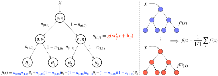
Figure 1: Schematic diagram of the functioning of Oblique Decision Forests. (Left): We illustrate the computation of a soft-routed oblique tree output $f^{t}(\mathbf{x})$ using individual tree node outputs. We observe that the final tree decision is composed of individual node outputs. (Right): We showcase how decisions from multiple oblique trees are combined to form $f(\mathbf{x})$.

3 Aranyani: Fair Oblique Decision Forests

In this section, we present Aranyani, a framework to enhance group fairness in decisions made during online learning. In this work, we focus on the group fairness notion of statistical or demographic parity. Our framework can be easily extended to other notions of group fairness, such as equalized odds (Hardt et al., 2016), equal opportunity (Hardt et al., 2016), and representation parity (Hashimoto et al., 2018) as described in Appendix B.1.

3.1 Problem Formulation

We describe the online learning setup where input instances arrive incrementally $\{\mathbf{x}_{1},\mathbf{x}_{2},\ldots\}$, with $\mathbf{x}_{t}$ arriving at time step $t$. The overall goal of the oblique decision forest $f$ is to make accurate decisions w.r.t. the task, $y$ (e.g., hiring decisions) while being fair w.r.t. the protected attribute, $a$ (e.g., gender). At time step $t$, the prediction model outputs a prediction $\hat{y}_{t}$ based on $f(\mathbf{x}_{t})$, where $\hat{y}_{t}=f(\mathbf{x}_{t})$ for regression and $\hat{y}_{t}=\operatorname*{arg\,max}f(\mathbf{x})$ for classification. With a slight abuse of notation, we denote the decisions made for an instance $\mathbf{x}$ with protected attribute $a=k$ as $f(\mathbf{x}|a=k)$ (forest output) or $n(\mathbf{x}|a=k)$ (node output), where $k=\{0,1\}$. Following previous work in fair online learning (Zhang & Ntoutsi, 2019), we consider the setup where the model receives both the true label $y_{t}$ and demographic label $a_{t}$ of an instance $\mathbf{x}_{t}$ after the prediction $\hat{y}_{t}$ has been made. The model can then use this feedback to update its parameters. Apart from achieving good performance on the task (a.k.a. high accuracy), we want the predictions made by the model to be fair across different groups. In the rest of this paper, we focus on demographic parity:

$$\mathrm{DP}=|\mathbb{E}[f(\mathbf{x}|a=0)]-\mathbb{E}[f(\mathbf{x}|a=1)]|.$$ (1)

Note that in the above definition, we consider a slightly modified version of demographic parity to handle scenarios where the preferred outcome (or target label) is not explicitly defined. For simplicity, we describe our system using a binary protected attribute $a\in\{0,1\}$, however, it can handle protected attributes with multiple classes ($>$2) as well (see more details in Appendix B.2).

3.2 Offline Setting

We begin by describing the simpler offline setting, in which all the training data is accessible prior to making predictions. In this setting, $f$ is optimized using stochastic gradient descent in a batch-wise manner. The constrained objective function is shown below:

$$\min_{f}\mathcal{L}(f(\mathbf{x}),y),\text{ subject to }\left|\mathbb{E}[f(\mathbf{x}|a=0)]-\mathbb{E}[f(\mathbf{x}|a=1)]\right|<\epsilon,$$ (2)

where $\mathcal{L}(\cdot,\cdot)$ is the task loss function (e.g., cross entropy loss) and $y$ is the true task label. The non-convex and non-smooth nature of the fairness objective (L1-norm in the DP term) makes it difficult to optimize the group fairness loss.

When $f$ is an oblique decision forest, we leverage its hierarchical prediction structure to impose group fairness constraints on the local node-level outputs, $n_{ij}(\mathbf{x})$ ($j$-th node at depth $i$) of the tree. The rationale behind applying constraints at the node outputs stems from the observation that if instances from different groups receive similar decisions at every node, then the final decision (which is an aggregation of the local decisions, Definition 2) is expected to be similar. We can formulate the node-level fairness constraints ($\mathcal{F}_{ij}$) as shown below:

$$\min_{f}\mathcal{L}(f(\mathbf{x}),y),\text{ s.t. }\forall({i,j})\;|\mathcal{F}_{ij}|<\epsilon,\text{ where }\mathcal{F}_{ij}=\mathbb{E}[n_{ij}(\mathbf{x}|a=0)]-\mathbb{E}[n_{ij}(\mathbf{x}|a=1)].$$ (3)

The node constraints $|\mathcal{F}_{ij}|$ are applied to all nodes (indexed by $(i,j)$) in the tree. We discuss the relation between node-level constraints and group fairness in Section 4. We note that $\mathcal{F}_{ij}$ is a function of the parameters of the $(i,j)$-th node only. In practice, we observe that this parameter isolation (Rusu et al., 2016) achieved by imposing fairness constraints on the local node-level outputs makes it easier to optimize $f$. We would like to emphasize that Aranyani can be extended to other notions of group fairness by modifying the formulation of $\mathcal{F}_{ij}$ (see Appendix B.1).

However, the optimization procedure in Equation 3 is hard to solve. We relax it by using a smooth surrogate for the L1-norm and turning the constraint into a regularizer. In particular, we use Huber loss function (Huber, 1992) (with hyperparameter $\delta>0$) and the relaxed optimization objective is:

$$\min_{f}\left\{\mathcal{L}(f(\mathbf{x}),y)+\lambda\sum_{i,j}H_{\delta}(\mathcal{F}_{ij})\right\},\text{ where }\;H_{\delta}(\mathcal{F}_{ij}):=\begin{cases}\mathcal{F}_{ij}^{2}/2,&\text{if }|\mathcal{F}_{ij}|<\delta\\ \delta|\mathcal{F}_{ij}-\delta/2|,&\text{otherwise}\end{cases},$$ (4)

with $\lambda$ being a hyperparameter. In the offline setting, the expectations over input instances in $\mathcal{F}_{ij}$ (Equation 3) are computed using samples within a training batch. In the online setup, computing these expectations is challenging as we only have access to individual instances at a time and not to a batch. Therefore, naively optimizing Equation 3 or 4 in the online setup requires storing all (or at least a subset) of the input instances. Moreover, we need to perform additional forward and backward passes for all stored instances to compute the group fairness gradients. In practice, this can be quite expensive in the online setting. In the following section, we discuss how to efficiently compute these group fairness gradients in the online setting.

3.3 Online Setting

In this section, we describe the training process for Aranyani in the online setting. As noted in the previous section, computing the expectations in group fairness terms is challenging due to storage and computational costs. Note that storing or processing previous input instances may pose challenges in several practical applications that need to adhere to privacy guidelines (Voigt & Von dem Bussche, 2017) or involve distributed infrastructure, such as federated learning (Konečnỳ et al., 2016). However, we do not need to compute the loss exactly using previous input instances as we only need the gradients of the loss function in order to update the model. We show that it is possible to estimate the fairness gradients by maintaining aggregate statistics of the node-level outputs in the tree. Taking the derivative of Equation 4, with respect to node parameters $\Theta\in[\mathbf{W},\mathbf{B}]$ of model $f$, we get the following gradients:

$$G(\Theta)=\nabla_{\Theta}\mathcal{L}(f(\mathbf{x}),y) +\lambda\sum_{\forall i,j}\nabla_{\Theta}H_{\delta}(\mathcal{F}_{ij}),$$ (5)

$$\text{where }\nabla_{\Theta}H_{\delta}{(\mathcal{F}_{ij})}=\begin{cases}\mathcal{F}_{ij}\nabla_{\Theta}\mathcal{F}_{ij},&\text{if }|\mathcal{F}_{ij}|<\delta\\ \delta\mathrm{sgn}\left(\mathcal{F}_{ij}-{\delta/}{2}\right)\nabla_{\Theta}\mathcal{F}_{ij},&\text{otherwise}\end{cases}$$

$$\text{and }\nabla_{\Theta}\mathcal{F}_{ij}=\mathbb{E}[\nabla_{\Theta}n_{ij}(\mathbf{x}|a=0)]-\mathbb{E}[\nabla_{\Theta}n_{ij}(\mathbf{x}|a=1)].$$

In the above equation, we have an unbiased estimate of the task gradient: $\nabla_{\Theta}\mathcal{L}(f(\mathbf{x}),y)$ for an i.i.d. sample $\mathbf{x}$. The fairness gradient $\nabla_{\Theta}H_{\delta}(\mathcal{F}_{ij})$ can be estimated by maintaining a number of aggregate statistics at each decision tree node. Specifically, we need to store the following aggregate statistics: (a) $\mathbb{E}[n_{ij}(\mathbf{x}|a=k)]$ and (b) $\mathbb{E}[\nabla_{\Theta}n_{ij}(\mathbf{x}|a=k)],\forall k$, where $k\in\{0,1\}$ denotes different protected attribute labels. In practice, for every incoming sample $\mathbf{x}_{t}$ we compute $n_{ij}(\mathbf{x}_{t})$ and $\nabla_{\Theta}n_{ij}(\mathbf{x}_{t})$, and update the aggregate statistics based on the protected label $a_{t}$. We denote the node constraints and gradients estimated using aggregate statistics as $\widehat{\mathcal{F}}_{ij}$ and $\widehat{G}(\Theta)$ respectively.

Note that in this setup, we do not need to store the previous input instances or query $f$ multiple times. Furthermore, computing $n_{ij}(\mathbf{x})$ and $\nabla_{\Theta}n_{ij}(\mathbf{x})$ is relatively inexpensive. For sigmoid functions, both $n_{ij}(\mathbf{x})$ and $\nabla_{\Theta}n_{ij}(\mathbf{x})$ can be obtained using a forward pass as: $\nabla_{\Theta}n_{ij}(\mathbf{x})=n_{ij}(\mathbf{x})(1-n_{ij}(\mathbf{x}))$. We discuss several properties of the estimated gradient $\widehat{G}(\Theta)$ in Section 4.

3.4 Training Procedure

In this section, we present an efficient training strategy for Aranyani. In general, tree-based architectures are slow to train using gradient descent as gradients need to propagate from leaf nodes to other nodes in a sequential fashion. We introduce a parameterization that enables us to compute oblique tree outputs only using matrix operations. This enables training on modern accelerators (like GPUs or TPUs) and helps us to efficiently compute task gradients (Equation 5) by using state-of-the-art autograd libraries. We begin by noting that all tree node outputs are independent of each other given the input $\mathbf{x}$. Therefore, the node outputs can be computed in parallel as shown below:

$$\mathbf{N}=g(\mathbf{W}^{T}\mathbf{x}+\mathbf{B})\in\mathbb{R}^{m},\text{where }\mathbf{W}\in\mathbb{R}^{m\times d},\mathbf{B}\in\mathbb{R}^{m}$$

and $m=2^{h}-1$ is the number of internal nodes (for a complete binary tree). Subsequently, these node outputs are utilized to calculate the probabilities required to reach individual leaf nodes. The path probabilities are computed by creating $2^{h}$ (number of leaf nodes) copies of the node outputs, $\overline{\mathbf{N}}=\begin{pmatrix}\mathbf{N},&\mathbf{N},&\cdots&,\mathbf{N}\end{pmatrix}\in\mathbb{R}^{m\times 2^{h}}$, and applying a mask, $\mathbf{A}$, that selects the ancestors for each leaf node. Each element of the mask $\mathbf{A}_{ij}\in\{-1,0,1\}$ selects whether the leaf path from a selected node is left (1), right (-1), or doesn’t exist (0). The exact probabilities are then stored in $\mathbf{P}$. This sequence of operations is shown below:

$$f(\mathbf{x})=\exp{(\mathbf{1}_{1\times m}\log\mathbf{P})}\mathbf{\Theta},\text{ where }\mathbf{P}=\mathrm{ReLU}(\overline{\mathbf{N}}\odot\mathbf{A})+(\mathbf{1}_{m\times 2^{h}}-\mathrm{ReLU}(-\overline{\mathbf{N}}\odot\mathbf{A}))$$

and $\mathbf{\Theta}\in\mathbb{R}^{2^{h}\times c}$. The selected probabilities can be utilized to compute the final output as $f(\mathbf{x})$. More details about the construction of mask $\mathbf{A}$ is reported in Appendix C.3.

4 Theoretical Analysis

In this section, we theoretically analyze several properties of Aranyani. In our proofs, we make assumptions that are standard in the optimization literature such as compact parameter set, Lipschitz task loss, bounded input $\mathbf{x}$, and bounded gradient noise (see Appendix A.1 for more details). First, we discuss the conditions of the node-level decisions and how they relate to group fairness constraints. Second, we analyze the properties of the gradient estimates (Equation 5) and show that the expected gradient norm converges for small step size and large enough time steps.

Lemma 1 (Demographic Parity Bound).

Let $f(\mathbf{x})$ be a soft-routed oblique decision tree of height $h$ with $\|\theta_{l}\|=1$ and assume an equal number of input instances $\mathbf{x}$ for each group of a binary protected attribute $a\in\{0,1\}$. Then, if all the node-level decisions satisfy the following condition:

$$\mathbb{E}[|n_{ij}(\mathbf{x}|a=0)-n_{ij}(\mathbf{x}|a=1)|]\leq\epsilon,\;\forall(i,j).$$ (6)

Then, the overall demographic parity of $f(\mathbf{x})$ is bounded as: $\mathrm{DP}\leq h2^{h}\epsilon$, for $\epsilon>0$.

The above lemma (proof in Appendix A.2) provides the node-level constraint (Equation 6) that upper bounds the demographic parity. We note that the node constraint $|\mathcal{F}_{ij}|$ (Equation 4) is a weaker constraint than the one derived above. The rationale behind using $\mathcal{F}_{ij}$ over the derived constraint is based on two key considerations: First, the expectation is computed using sample pairs from complementary groups (in Equation 6), which is challenging to compute in both offline and online settings. Second, optimizing this constraint can severely limit the task performance as it encourages the trivial solution of having the same node outputs for all instances.

Next, we derive the Rademacher complexity of soft-routed decision trees. Empirical Rademacher complexity, $\hat{R}_{n}(\mathcal{H})$, measures the ability of function class $\mathcal{H}$ to fit random noise indicating its expressivity (formal definition and proof in Appendix A.3).

Lemma 2 (Rademacher Complexity).

Empirical Rademacher complexity, $\hat{R}_{n}(\mathcal{H})$, for soft-routed decision tree (of height $h$) function class, $f(\mathbf{x})\in\mathcal{H}$, and $\|\theta_{l}\|=1$ is bounded as: $\hat{R}_{n}(\mathcal{H})\leq{2^{h}/}{\sqrt{n}}$.

We observe that the bound exponentially increases with the height of the tree, $h$. Interestingly, according to the DP bound in Equation 6, it appears that we can easily improve group fairness by using a shallower tree (smaller $h$). This illustrates the trade-off between fairness and accuracy, highlighting that it is not feasible to enhance group fairness without a substantial impact on accuracy.

Next, we derive the estimation error bound for the gradients (in Equation 5), which stems from the fact that we use aggregate statistics of node outputs from previous time steps where the model parameters were different. First, we derive the estimation error bounds for the aggregate statistics $\mathcal{\widehat{F}}_{ij}$ and $\nabla\mathcal{\widehat{F}}_{ij}$ (Lemma 4). Using these results, we bound the estimation error of fairness gradients $\nabla_{\Theta}H_{\delta}(\mathcal{\widehat{F}}_{ij})$ in the following lemma (proof in Appendix A.4).

Lemma 3 (Fairness Gradient Estimation Error).

For a soft-routed oblique decision tree $f(\mathbf{x})$ with $L_{g}$-smooth activation function $g(\cdot)$, bounded i.i.d. input instances $\|\mathbf{x}_{t}\|\leq B$, and compact parameter set $\Theta_{t}\in\mathcal{B_{F}}(0,R)$ (Frobenius norm ball of radius $R$), the estimation error can be bounded:

$$\|\nabla_{\Theta}H_{\delta}(\mathcal{F}_{ij})-\nabla_{\Theta}H_{\delta}(\widehat{\mathcal{F}}_{ij})\|\leq{\delta B}/{2},$$ (7)

where $\delta$ is the Huber loss parameter (Equation 4).

Next, we use the above bound to derive the convergence of biased gradients building on the results from Ajalloeian & Stich (2020) to obtain the following result (proof in Appendix A.5):

Theorem 1 (Gradient Norm Convergence).

Using the assumptions in Lemma 3, the expected gradient norm $\Psi_{T}={1}/{T}\sum_{t=0}^{T-1}\mathbb{E}[\|\widehat{G}(\Theta_{t})\|^{2}]$ can be bounded as: $\Psi_{T}\leq\left(\epsilon+{2^{2h-2}\lambda^{2}\delta^{2}B^{2}}\right)$, for large enough time step $T\geq\max\left(\frac{4FL(M+1)}{\epsilon},\frac{4FL\sigma^{2}}{\epsilon^{2}}\right)$, small step size $\gamma\leq\min\left(\frac{1}{(M+1)L},\frac{\epsilon}{2L\sigma^{2}}\right)$ and $\epsilon>0$ (see definitions in Appendix A.5).

The above bound demonstrates that the expected norm of the gradients estimated using the aggregate statistics of decisions from previous time steps converges over time (see Appendix A.5). In the following sections, we perform experiments to empirically verify the theoretical results.

5 Experiments

In this section, we present the details of our experimental setup and results to evaluate Aranyani.

Baselines. We compare Aranyani with the following online learning algorithms: Hoeffding Trees (HT) (Domingos & Hulten, 2000) performs decision tree learning for online data streams by leveraging the Hoeffding bound (Hoeffding, 1994), Adaptive Hoeffding Trees (AHT) (Bifet & Gavalda, 2009) improves upon HTs by detecting changes in the input data stream and updating the learning process accordingly, FAHT (Zhang & Ntoutsi, 2019) modifies the HT splitting algorithm by introducing group fairness constraints while computing the Hoeffding bound, MLP Aranyani, (MLP), uses an MLP as $f(\mathbf{x})$ and the same online learning updates described in Section 3.3 (more details about the architecture in Appendix C), Leaf Aranyani (Leaf) stores the aggregate gradient statistics w.r.t. leaf-level predictions or the final output instead of the node predictions, Majority is a post-processing baseline considers the output of $f(\mathbf{x})$ with probability $p$ and outputs the majority label with $(1-p)$ probability. We report the results for different values of $p$. The majority baseline can provide a fairness improvement by simply decreasing the task performance, but it requires prior access to target label information. In practice, outperforming the majority baseline is not easy. As pointed out by (Lowy et al., 2022), many offline techniques fall short of the majority’s performance when batch sizes are small, which is consistent with the online learning setup.

Online Setup & Evaluation. We use the online learning setup described in Section 3.1. For each algorithm, we retain predictions $\hat{y}_{t}$ from every step and report the average task performance (accuracy) and demographic parity. In all experiments (unless otherwise stated), we use oblique forests with 3 trees and each tree has a height of 4 (based on a hyperparameter grid search). We provide further details in Appendix C. Next, we present the evaluation results of fair online learning using Aranyani and other baselines on 3 tabular datasets, a vision, and a language-based dataset.

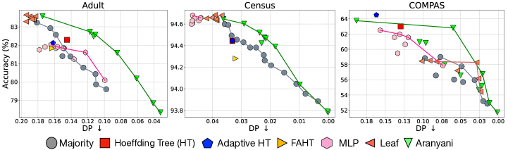
Figure 2: We report the group fairness (demographic parity) vs. task performance (accuracy) trade-off plots for different systems in (left) Adult, (center) Census, and (right) COMPAS datasets. Ideally, a fair online system should achieve low demographic parity along with high accuracy scores. Considering the inverted $x$-axis, the performance of a fair system should lie in the top right quadrant of each plot. We observe that Aranyani’s performance for different $\lambda$’s and observe that it achieves better accuracy-fairness trade-off compared to baseline systems.

5.1 Tabular Datasets

We conducted our experiments on the following tabular datasets: (a) UCI Adult (Becker & Kohavi, 1996), (b) Census (Dua et al., 2017), and (c) ProPublica COMPAS (Angwin et al., 2016). Adult dataset contains 14 features of $\sim$48K individuals. The task involves predicting whether the annual income of an individual is more than $50K or not and the protected attribute is gender. Census dataset has the same task description but contains 41 attributes for each individual and 299K instances. Propublica COMPAS considers the binary classification task of whether a defendant will re-offend with the protected attribute being race. COMPAS has $\sim$7K instances.

Figure 2 demonstrates the group fairness-accuracy trade-off, where $x$ and $y$-axis show the average demographic parity and accuracy scores respectively. Ideally, we want an online system to achieve low demographic parity and high accuracy, making the top-right quadrant of the plot the desired outcome ($x$-axis is inverted). We report Aranyani’s performance for different $\lambda$ values (Equation 5), which controls the fairness-accuracy trade-off. We observe that Aranyani’s results lie in the top-right portion, showcasing that it can achieve the best trade-off. We also observe that the improvement of Aranyani over baseline methods is least pronounced in COMPAS. This could be because COMPAS has fewer instances compared to the other datasets, potentially affecting convergence.

We also assess the significance of the tree structure in Aranyani by examining the Aranyani MLP baseline that employs the same gradient accumulation method discussed in Section 3.3, but without the tree structure. In all datasets, we observe that the MLP baseline is unable to improve the fairness scores beyond a certain point. Upon further investigation, we found that this phenomenon happens due to the vanishing fairness gradients in the layers further from the output. We also observe the same phenomenon for Leaf baseline, where the fairness gradients for nodes away from the leaves become very small and they cannot be trained effectively. This showcases the importance of parameter isolation in Aranyani and the application of group fairness constraints on local decisions. We also note that the conventional Hoeffding tree-based baselines (HT , AHT , and FAHT ) achieve poor fairness scores, often falling behind majority post-processing, which shows that HT based approaches are unable to robustly improve the group fairness. Overall, we observe that Aranyani can achieve a better accuracy-fairness trade-off than baseline approaches across all datasets.

5.2 Vision & Language Datasets

We also conduct experiments on (a) CivilComments (Do, 2019) toxicity classification and (b) CelebA (Liu et al., 2015) image classification datasets. CivilComments is a natural language dataset where the task involves classifying whether an online comment is toxic or not. We use religion as the protected attribute and consider instances of religion labels: “Muslim” and “Christian”, as they showcase the maximum discrepancy in toxicity. For CivilComments, we obtain text representations from the instruction-tuned model, Instructor (Su et al., 2022) by using the prompt “Represent a toxicity comment for classifying its toxicity as toxic or non-toxic: [comment]”. CelebA dataset contains 200K images of celebrity faces with 40 categorical attributes. Following previous works (Jung et al., 2022b; Qiao & Peng, 2022; Jung et al., 2022a; Liu et al., 2021), we select “blond hair” as the task label and “gender” as the protected attribute. For CelebA, we retrieve the image representations from the CLIP model (Radford et al., 2021).

In Figure 3, we report the fairness-accuracy trade-off plots for the above datasets. We observe that Aranyani achieves the best accuracy-fairness trade-off on both datasets. Similar to tabular datasets, we observe that the MLP and Leaf baselines are unable to improve the fairness scores at all. The Hoeffding tree (HT) baseline achieves subpar accuracy scores on both datasets. It achieves decent fairness scores as it is unable to converge on the task. This highlights the limitations of traditional decision trees when dealing with non-axis-aligned data.

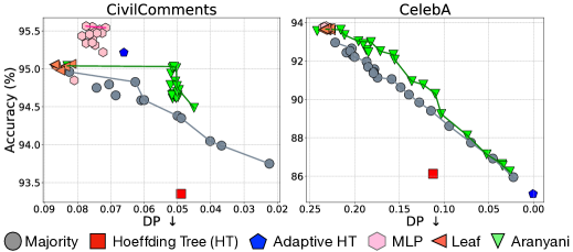
Figure 3: We report the group fairness vs. accuracy trade-off plots for different systems in (left) CivilComments and (right) CelebA datasets. We observe that Aranyani achieves significantly better accuracy-fairness trade-off than baseline systems.

5.3 Analysis

In this section, we perform empirical evaluations to analyze the functioning of Aranyani.

Reservoir Variant. We compare the performance of Aranyani with a variant (using oblique forests) that stores all samples in the online stream to compute the fairness loss. We refer to this variant as “Reservoir”. In Figure 4 (left), we observe that Aranyani achieves a similar accuracy-fairness tradeoff compared to the reservoir variant on the Adult dataset. As Aranyani does not need to store previous input samples, it is quite efficient – achieving a $\sim$3x improvement in computation time and $\sim$23% reduction in memory utilization.

Gradient Convergence. We investigate the convergence of the gradients used to update the oblique tree. We conduct our experiment on CivilComments dataset using Aranyani with a single tree and report the norm of the total gradients and fairness gradients used to update $\mathbf{W}$ (weight parameter of each node). In Figure 4 (center), we observe that the norm of both task and fairness gradients converge over time during the online learning process. This corroborates our theoretical guarantees in Lemma 1. We found this behavior to be consistent across different parameters (Appendix D).

Tree Height Ablations. We study the effect of varying the tree height in oblique forests on the fairness-accuracy tradeoff. In Figure 4 (right), we report Aranyani’s performance on the Adult dataset with a fixed parameter $\lambda=0.1$. We observe that the accuracy increases with height and the demographic parity worsens ($y$-axis is inverted) with increasing height. This is consistent with our theoretical results (Lemma 1 & 2). However, we have observed a slight decrease in accuracy when using large tree heights (height=8). This observation suggests that oblique trees may overfit the training data when reaching a certain height, and choosing a shallower tree could be beneficial. We perform additional experiments to investigate the performance of Aranyani (see Appendix D).

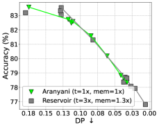
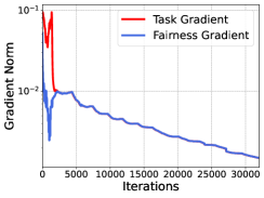
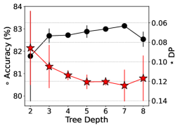
Figure 4: (left) We compare Aranyani with the reservoir variant that stores all input instances, (center) we investigate the gradient convergence, and (right) the impact of tree height on performance.

6 Related Works

Fairness. Existing work on promoting group fairness can be classified into three categories: pre-processing (Zemel et al., 2013; Calmon et al., 2017), post-processing (Hardt et al., 2016; Pleiss et al., 2017; Alghamdi et al., 2022), and in-processing (Quadrianto & Sharmanska, 2017; Agarwal et al., 2018; Mary et al., 2019; Prost et al., 2019; Baharlouei et al., 2020; Lahoti et al., 2020; Lowy et al., 2022; Basu Roy Chowdhury et al., 2021; Chowdhury & Chaturvedi, 2022) techniques. These are trained and tested on a static dataset, and there is a growing concern that they fail to remain fair under distribution shifts (Barrett et al., 2019; Mishler & Dalmasso, 2022; Rezaei et al., 2021; Wang et al., 2023). This calls for the development of fairness-aware systems that can adapt to distribution changes and update themselves in an online manner. However, an online learning setting, where input instances arrive one at a time, presents several challenges that make it difficult to apply existing techniques: (a) pre-processing techniques are not feasible as they require prior access to input instances; (b) post-processing techniques often require access to a held-out set, which may be impractical; and (c) in-processing approaches need to store previous input instances to estimate the group fairness loss, which may not always be feasible due to privacy reasons (Voigt & Von dem Bussche, 2017) or distributed infrastructure (Konečnỳ et al., 2016). Although several works (Gillen et al., 2018; Bechavod et al., 2020) have studied individual fairness in online settings, only a few recent works (Chowdhury & Chaturvedi, 2023; Zhao et al., 2023) considered group fairness in settings where the underlying task or data distribution changes over time. However, these systems are incrementally trained on sub-tasks, necessitating access to task labels. Consequently, they are unable to process online data streams.

Decision Trees. Decision trees have been studied for the online setting where data arrives in a stream over time, particularly to mitigate catastrophic forgetting (Kirkpatrick et al., 2017). Initial works (Kamiran et al., 2010; Raff et al., 2018; Aghaei et al., 2019) explored various formulations of the splitting criterion to improve fairness in decision trees within the offline setting. More recent work (Zhang & Ntoutsi, 2019) in fair online learning leveraged Hoeffding trees (Domingos & Hulten, 2000) to process online data streams, and introduced group fairness constraints in its splitting criteria. However, this approach has several drawbacks: (a) conventional decision trees can only function with axis-aligned data making it unsuitable for more complex data domains like text or images, (b) it cannot be trained using gradient descent making it difficult to plug in additional modules like a text or image encoder. In contrast to these approaches, Aranyani leverages oblique decision trees parameterized by neural networks improving its expressiveness while making it amenable to gradient-based updates using modern accelerators. Aranyani exploits its tree structure to store aggregate statistics of the local node outputs to compute the fairness gradients without requiring it to store additional samples.

Gradient-based learning of trees. Aranyani uses a gradient-based objective to discover the tree-structured classifier. Most similar to our work (Karthikeyan et al., 2022) uses gradient-based methods to discover the structure of oblique decision tree classifiers. Discovering tree structures with gradient-based methods has been also considered in works on autoencoders (Nagano et al., 2019; Shin et al., 2016), on discovering structure (e.g., parses) in natural language (Yin et al., 2018; Drozdov et al., 2019), hierarchical clustering (Monath et al., 2017; 2019; Zhao et al., 2020; Chami et al., 2020), phylogenetics (Macaulay & Fourment, 2023; Penn et al., 2023), and extreme classification (Yu et al., 2022; Jernite et al., 2016; Sun et al., 2019; Jasinska-Kobus et al., 2021).

7 Conclusion

In this paper, we propose Aranyani, a framework to achieve group fairness in online learning. Aranyani uses an ensemble of oblique decision trees and leverages its hierarchical prediction structure to store aggregate statistics of local decisions. These aggregate statistics help in the efficient computation of group fairness gradients in the online setting, eliminating the need to store previous input instances. Empirically, we observe that Aranyani achieves significantly better accuracy-fairness trade-off compared to baselines on a wide range of tabular, image, and text classification datasets. Through extensive analysis, we showcase the utility of our proposed tree-based prediction structure and fairness gradient approximation. While we investigated binary oblique tree structures, their ability to fit complex functions can be limited when compared to fully connected networks. Future research can explore other parameterizations (e.g., graph-based structures) that enable effective gradient computation to impose group fairness in online settings with superior prediction power.

Reproducibility Statement

We have submitted the implementation of Aranyani in the supplementary materials. We have extensively discussed the details of our experimental setup, datasets, baselines, and hyperparameters in Section 5 and Appendix D. We have also provided the details of our training procedure in Section 3.4 and Appendix C.3. We will make our implementation public once the paper is published.

Ethics Statement

In this paper, we introduce an online learning framework, Aranyani, to enhance group fairness while making decisions for an online data stream. Aranyani has been developed with the intention of mitigating biases of machine learning systems when they are deployed in the wild. However, it is crucial to thoroughly assess the data’s quality and the accuracy of the demographic labels used for training Aranyani, as otherwise, it may still encode negative biases. In our experiments, we use publicly available datasets and obtain data representations from open-sourced models. We do not obtain any demographic labels through data annotation or any private sources.

Appendix A Theoretical Proofs

A.1 Assumptions

In this section, we will present standard regularity assumptions utilized in deriving the theoretical results. We derive the results for a soft-routed oblique decision forest, $f(\mathbf{x})$, with a single tree, $|\mathcal{T}|=1$. However, these can be easily extended to a setup with multiple trees. Specifically, we derive the estimation errors in gradients leveraging the framework of Ajalloeian & Stich (2020), i.e., we assume our stochastic gradient estimation for the objective has the following form: $\widehat{G}(\Theta,\xi)=G(\Theta)+b(\Theta)+n(\xi)$, where $b(\Theta)$ and $n(\xi)$ denotes the bias and noise involved in the estimation. We present an exact description of all the assumptions used in our setup and optimization process:

1. The input instances $\mathbf{x}_{t}$ arrive in an i.i.d. fashion and are bounded: $\|\mathbf{x}_{t}\|<B$.

2. The parameter set is compact and lies within a Frobenius ball $\Theta\in\mathcal{B}_{F}(0,R)$ of radius $R$.

3. $f(\mathbf{x})$ denotes a soft-routed binary oblique forest with a single tree ($|\mathcal{T}|=1$), activation function, $g(\cdot)$, and leaf parameters $\|\theta_{l}\|=1$.

4. The activation function $g(\cdot)$ used in oblique trees is $L_{g}$ smooth.

5. The noise in gradient estimation $n(\xi)$ has zero mean $\mathbb{E}_{\xi}[n(\xi)]=\mathbf{0}$ and is $(M,\sigma^{2})$ bounded:

   $$\mathbb{E}_{\xi}[\|n(\xi)\|^{2}]\leq M\|G(\Theta)+b(\Theta)\|^{2}+\sigma^{2},\forall\Theta.$$ (8)

6. The task loss function $\mathcal{L}(\cdot,\cdot)$ is $K_{t}$-Lipschitz.

A.2 Proof of Lemma 1

First, we present a proposition that would help prove Lemma 1.

Proposition 1.

Let $p_{i}$ and $q_{i}$ be samples from a random variable $P$ that is bounded between $[0,1]$. Then, the following inequality holds:

$$\left|\prod_{i}p_{i}-\prod_{i}q_{i}\right|\leq\sum_{i}|q_{i}-p_{i}|.$$ (9)

Proof.

The proof is presented below:

$$\left|\prod_{i}p_{i}-\prod_{i}q_{i}\right| \leq\prod_{i}\max\{p_{i},q_{i}\}-\prod_{i}\min\{p_{i},q_{i}\}$$

$$\leq\sum_{i}|q_{i}-p_{i}|\prod_{j\neq i}\max\{p_{j},q_{j}\}$$

$$\leq\sum_{i}|q_{i}-p_{i}|.$$

∎

Next, we proceed to the main proof of Lemma 1.

Proof of Lemma 1.

The proof is completed using the following steps:

$$\mathrm{DP} =\left|\mathop{\mathbb{E}}[f(\mathbf{x}|a=0)]-\mathop{\mathbb{E}}[f(\mathbf{x}|a=1)]\right|$$

$$=\left|\mathop{\mathbb{E}}\left[\sum_{l}p_{l}(\mathbf{x}|a=0)\theta_{l}\right]-\mathop{\mathbb{E}}\left[\sum_{l}p_{l}(\mathbf{x}|a=1)\theta_{l}\right]\right|$$

$$=\left|\sum_{l}\left(\mathop{\mathbb{E}}\left[p_{l}(\mathbf{x}|a=0)\right]-\mathop{\mathbb{E}}\left[p_{l}(\mathbf{x}|a=1)\right]\right)\theta_{l}\right|$$

$$\leq\sum_{l}\left|\mathop{\mathbb{E}}\left[p_{l}(\mathbf{x}|a=0)\right]-\mathop{\mathbb{E}}\left[p_{l}(\mathbf{x}|a=1)\right]\right||\theta_{l}|$$

$$=\sum_{l}\left|\mathop{\mathbb{E}}\left[\prod_{i}n_{i,A(i,l)}(\mathbf{x}|a=0)\right]-\mathop{\mathbb{E}}\left[\prod_{i}n_{i,A(i,l)}(\mathbf{x}|a=1)\right]\right|$$

$$=\sum_{l}\left|\frac{1}{m}\sum_{\mathbf{x}_{0}\sim p(\mathbf{x}|a=0)}\left[\prod_{i}n_{i,A(i,l)}(\mathbf{x}_{0})\right]-\frac{1}{m}\sum_{\mathbf{x}_{1}\sim p(\mathbf{x}|a=1)}\left[\prod_{i}n_{i,A(i,l)}(\mathbf{x}_{1})\right]\right|$$

$$=\sum_{l}\left|\frac{1}{m}\sum_{\mathbf{x}_{0}\sim p(\mathbf{x}|a=0),\mathbf{x}_{1}\sim p(\mathbf{x}|a=1)}\left(\prod_{i}n_{i,A(i,l)}(\mathbf{x}_{0})-\prod_{i}n_{i,A(i,l)}(\mathbf{x}_{1})\right)\right|$$

$$\leq\sum_{l}\frac{1}{m}\sum_{\mathbf{x}_{0},\mathbf{x}_{1}}\sum_{i}\left|n_{i,A(i,l)}(\mathbf{x}_{0})-n_{i,A(i,l)}(\mathbf{x}_{1})\right|$$ (10)

$$=\sum_{l}\sum_{i}\mathbb{E}\left[\left|n_{i,A(i,l)}(\mathbf{x}_{0})-n_{i,A(i,l)}(\mathbf{x}_{1})\right|\right]$$ (11)

$$\leq\sum_{l}\sum_{i}\epsilon$$

$$=h2^{h}\epsilon.$$

In the above proof, the first few steps use the linearity of expectation. We derive Equation 10 by using the result in Proposition 9. Finally, plugging the bound from Equation 6 in Equation 11 we obtain the final result. ∎

A.3 Proof of Lemma 2

First, we present the definition of empirical Rademacher complexity, $\hat{R}_{n}(\mathcal{H})$, for function class, $\mathcal{H}$.

$$\hat{R}_{n}(\mathcal{H})\vcentcolon=\frac{1}{n}\mathbb{E}_{\epsilon}\left[\sup_{h\in\mathcal{H}}\sum_{t=1}^{n}\epsilon_{t}f(\mathbf{x}_{t})\right].$$ (12)

Intuitively, the above definition measures the expressivity of a function class $\mathcal{H}$ by measuring the ability to fit random noise. In the above equation, for a given set $S=\{\mathbf{x}_{1},\ldots,\mathbf{x}_{n}\}$ and Rademacher vector $\epsilon$, the supremum quantifies the maximum correlation between $f(\mathbf{x}_{t})$ and randomly generated samples $\epsilon_{t}\in\{-1,1\}$ $\forall f\in\mathcal{H}$.

Proof.

In Equation 12, we plug in the soft-routed binary oblique decision tree formulation, $f(\mathbf{x})=\sum_{l=1}^{2^{h}}\prod_{i=1}^{h}g(\mathbf{w}_{i,A(i,l)}^{T}\mathbf{x}+\mathbf{b}_{i,A(i,l)})\theta_{l}$, in the above equation to obtain:

$$\hat{R}_{n}(\mathcal{H}) =\frac{1}{n}\mathbb{E}_{\epsilon}\left[\sup_{h\in\mathcal{H}}\sum_{t=1}^{n}\epsilon_{t}\sum_{l=1}^{2^{h}}\prod_{i=1}^{h}g(\mathbf{w}_{i,A(i,l)}^{T}\mathbf{x}_{t}+\mathbf{b}_{i,A(i,l)})\theta_{l}\right]$$

$$\leq\frac{2^{h}}{n}\mathbb{E}_{\epsilon}\left[\sup_{h\in\mathcal{H}}\max_{l}\sum_{t=1}^{n}\epsilon_{t}\prod_{i=1}^{h}g(\mathbf{w}_{i,A(i,l)}^{T}\mathbf{x}_{t}+\mathbf{b}_{i,A(i,l)})\theta_{l}\right]$$

$$\leq\frac{2^{h}}{n}\mathbb{E}_{\epsilon}\left[\sup_{h\in\mathcal{H}}\sum_{t=1}^{n}\epsilon_{t}\max_{l}\prod_{i=1}^{h}g(\mathbf{w}_{i,A(i,l)}^{T}\mathbf{x}_{t}+\mathbf{b}_{i,A(i,l)})\theta_{l}\right].$$

Next, we continue the proof by using $F(\mathbf{x}_{t})=\max_{l}\prod_{i=1}^{h}g(\mathbf{w}_{i,A(i,l)}^{T}\mathbf{x}_{t}+\mathbf{b}_{i,A(i,l)})\theta_{l}$ and $\|\theta_{l}\|=1$.

$$\hat{R}_{n}(\mathcal{H}) \leq\frac{2^{h}}{n}\mathbb{E}_{\epsilon}\left[\sup_{h\in\mathcal{H}}\sum_{t=1}^{n}\epsilon_{t}F(\mathbf{x}_{t}))\right]$$

$$\leq\frac{2^{h}}{n}\sqrt{\sup_{h\in\mathcal{H}}\mathbb{E}_{\epsilon}\left[\left\|\sum_{t=1}^{n}\epsilon_{t}F(\mathbf{x}_{t})\right\|^{2}\right]}$$

$$=\frac{2^{h}}{n}\sqrt{\sup_{h\in\mathcal{H}}\mathbb{E}_{\epsilon}\left[\sum_{t=1}^{n}\epsilon_{t}^{2}F(\mathbf{x}_{t})^{2}\right]+\mathbb{E}_{\epsilon}\left[\sum_{t\neq t^{\prime}}\epsilon_{t}^{\prime}\epsilon_{t}F(\mathbf{x}_{t})F(\mathbf{x}_{t}^{\prime})\right]}$$

$$=\frac{2^{h}}{n}\sqrt{\mathbb{E}_{\epsilon}\left[\sum_{t=1}^{n}\epsilon_{t}^{2}\right]}$$

$$\leq 2^{h}/\sqrt{n}.$$

∎

A.4 Proof of Lemma 3

The proof of Lemma 3 builds on the intermediate results that we present in the sequel. First, we derive the bound on the estimation error in $\nabla\mathcal{\widehat{F}}_{ij}$. Using this result, we can bound the estimation in the fairness gradients derived in Equation 5.

For simplicity of notation, in the subsequent proof, we denote input instances from different demographic groups as $\mathbf{x}_{i}\sim p(\mathbf{x}|a=0)$ and $\mathbf{x}_{j}\sim p(\mathbf{x}|a=1)$. With a slight abuse of notation, we also use the indices $i,j$ to indicate the time step at which the instance $\mathbf{x}_{i}$ arrives.

Lemma 4 (Estimation error in $\nabla\mathcal{F}_{ij}$).

Under assumptions (A1), (A2), (A3), (A4), the estimation error of $\nabla\mathcal{F}_{ij}$ is bounded as: $|\nabla\mathcal{F}_{ij}-\nabla\widehat{\mathcal{F}}_{ij}|\leq\min\left\{{B}{/4},{2L_{g}R}\right\}$.

Proof.

Next, we focus on approximating the estimation error in $\nabla\mathcal{\widehat{F}}_{ij}$.

$$\nabla\mathcal{F}_{ij}=\mathbb{E}_{i}[\nabla n(\Theta_{t},\mathbf{x}_{i})]-\mathbb{E}_{j}[\nabla n(\Theta_{t},\mathbf{x}_{j})],\;\nabla\widehat{\mathcal{F}}_{ij}=\mathbb{E}_{i}[\nabla n(\Theta_{i},\mathbf{x}_{i})]-\mathbb{E}_{j}[\nabla n(\Theta_{j},\mathbf{x}_{j})].$$

In a similar manner, we can estimate the approximation error as:

$$|\nabla\mathcal{F}_{ij}-\nabla\widehat{\mathcal{F}}_{ij}| =|\mathbb{E}_{i}[\nabla n(\Theta_{t},\mathbf{x}_{i})]-\mathbb{E}_{i}[\nabla n(\Theta_{i},\mathbf{x}_{i})]-\mathbb{E}_{j}[\nabla n(\Theta_{t},\mathbf{x}_{j})]+\mathbb{E}_{j}[\nabla n(\Theta_{j},\mathbf{x}_{j})]|$$

$$=|\mathbb{E}_{i}[\nabla n(\Theta_{t},\mathbf{x}_{i})-\nabla n(\Theta_{i},\mathbf{x}_{i})]-\mathbb{E}_{j}[\nabla n(\Theta_{t},\mathbf{x}_{j})-\nabla n(\Theta_{j},\mathbf{x}_{j})]|$$

$$\leq|\mathbb{E}_{i}[\nabla n(\Theta_{t},\mathbf{x}_{i})-\nabla n(\Theta_{i},\mathbf{x}_{i})]|+|\mathbb{E}_{j}[\nabla n(\Theta_{t},\mathbf{x}_{j})-\nabla n(\Theta_{j},\mathbf{x}_{j})]|$$

$$=L_{g}\mathbb{E}_{i}[\|\Theta_{t}-\Theta_{i}\|]+L_{g}\mathbb{E}_{j}[\|\Theta_{t}-\Theta_{j}\|]$$

$$=L_{g}\mathbb{E}_{i}[\|\Theta_{t}-\Theta_{i}\|]$$

$$\leq 2L_{g}R,$$

where $L_{g}$ is the smoothness constant of the activation function. Note that this error bound doesn’t increase in an unrestricted manner as the node gradients are bounded as:

$$|\nabla n(\Theta_{t},\mathbf{x})|\leq\|\mathbf{x}\|/4\leq B/4.$$

Therefore, we can derive a tighter bound as:

$$|\nabla\mathcal{F}_{ij}-\nabla\widehat{\mathcal{F}}_{ij}|\leq\min\left\{\frac{B}{4},{2L_{g}R}\right\}.$$

For sigmoid activation, we can plug in $L_{g}=\frac{2\sqrt{3}-3}{18}$ in the above equation to get the exact bound. ∎

Using the bounds derived in the above lemmas, we proceed towards the proof of Lemma 3.

Proof of Lemma 3.

We begin by noting that the task loss gradients are unbiased as the input instance $\mathbf{x}_{t}$ is sampled in an i.i.d. fashion making the gradient estimate unbiased on expectation.

$$\|\nabla_{\Theta}H_{\delta}(\mathcal{F}_{ij}) -\nabla_{\Theta}H_{\delta}(\widehat{\mathcal{F}}_{ij})\|=$$

$$\begin{cases}\|\mathcal{F}_{ij}.\nabla_{\Theta}\mathcal{F}_{ij}-\widehat{\mathcal{F}}_{ij}\nabla_{\Theta}\widehat{\mathcal{F}}_{ij}\|,&\text{if }|\widehat{\mathcal{F}}_{ij}|<\delta\\ \delta\|\mathrm{sgn}\left(\mathcal{F}_{ij}-{\delta/}{2}\right)\nabla_{\Theta}\mathcal{F}_{ij}-\mathrm{sgn}\left(\widehat{\mathcal{F}}_{ij}-{\delta/}{2}\right)\nabla_{\Theta}\widehat{\mathcal{F}}_{ij}\|,&\text{otherwise}\end{cases}.$$

Therefore, the approximation error arises from the fairness gradient terms. First, we consider the approximation error in the gradients when $|\widehat{\mathcal{F}}_{ij}|\leq\delta$. It can be written as:

$$|\mathcal{F}_{ij}\nabla\mathcal{F}_{ij}-\widehat{\mathcal{F}}_{ij}\nabla\widehat{\mathcal{F}}_{ij}| \leq\delta|\nabla\mathcal{F}_{ij}-\nabla\widehat{\mathcal{F}}_{ij}|\leq\delta B/4.$$

Note that in the above equation, we consider the weaker upper bound for the estimation error of $\nabla\mathcal{F}_{ij}$ of $B/4$. As the bound on the input $\|\mathbf{x}\|\leq B$ is easier to work with. Next, we consider the case where $|\mathcal{F}_{ij}|>\delta$:

$$\delta|\mathrm{sgn}(\mathcal{F}_{ij}-\delta/2)\nabla\mathcal{F}_{ij}-\mathrm{sgn}(\widehat{\mathcal{F}}_{ij}-\delta/2)\nabla\widehat{\mathcal{F}}_{ij}| \leq\delta|2\nabla\mathcal{F}_{ij}|\leq\delta B/2.$$

Therefore, we observe that the overall error can be bounded as:

$$\|\nabla_{\Theta}H_{\delta}(\mathcal{F}_{ij})-\nabla_{\Theta}H_{\delta}(\widehat{\mathcal{F}}_{ij})\|\leq\delta B/2.$$ (13)

∎

A.5 Proof of Theorem 1

Theorem 2 (Precise Statement of Theorem 1).

Using the assumptions (A1), (A2), (A3), (A4), (A5), for $\epsilon>0$ the expected gradient norm $\Psi_{T}={1}/{T}\sum_{t=0}^{T-1}\mathbb{E}[\|\widehat{G}(\Theta_{t})\|^{2}]$ can be bounded as $\Psi_{T}\leq\left(\epsilon+{2^{2h-2}\lambda^{2}\delta^{2}B^{2}}\right)$ for

$$T\geq\max\left(\frac{4FL(M+1)}{\epsilon},\frac{4FL\sigma^{2}}{\epsilon^{2}}\right)\text{ and }\gamma\leq\min\left(\frac{1}{(M+1)L},\frac{\epsilon}{2L\sigma^{2}}\right).$$ (14)

where $F=\mathbb{E}[\mathcal{L}_{o}(\theta_{t})]-\mathcal{L}_{o}^{*}$ with $\mathcal{L}_{o}$ denoting the overall loss function (Equation 4).

Proof.

Due to estimation errors in the online setting, the gradients we use are biased and can be written as:

$$\widehat{G}(\Theta,\xi)=G(\Theta)+b(\Theta)+n(\xi)$$ (15)

where $G(\Theta)$ is the exact gradient (computed using all the input instances seen so far), $b(\Theta)$ is the bias or estimation error, and $n(\xi)$ is the noise coming from the i.i.d. estimate of the loss function. From Lemma 3, we can bound the overall estimation bias as:

$$\|b(\Theta)\|\leq\lambda\sum_{\forall i,j}\|\nabla_{\Theta}H_{\delta}(\mathcal{F}_{ij})-\nabla_{\Theta}H_{\delta}(\widehat{\mathcal{F}}_{ij})\|\leq 2^{h-1}\lambda\delta B.$$ (16)

and $n(\xi)$ has zero mean. We assume that the noise $n(\xi)$ is $(M,\sigma^{2})$ bounded as defined by Ajalloeian & Stich (2020). Note that $M$ depends on the task loss function $\mathcal{L}(\cdot,\cdot)$ and is not a function of $t$. We use the result from Lemma 2 in (Ajalloeian & Stich, 2020) to obtain:

$$\Psi_{T}\leq\frac{2F}{T\gamma}+{2^{2h-2}\lambda^{2}\delta^{2}B^{2}}+\gamma L\sigma^{2}$$ (17)

where we denote the average gradient norm as: $\Psi_{T}=\frac{1}{T}\sum_{t=0}^{T-1}\mathbb{E}[\|\widehat{G}(\Theta_{t})\|^{2}]$, $F=\mathbb{E}[\mathcal{L}_{o}(\Theta_{0})]-\mathcal{L}_{o}^{*}$ with $\mathcal{L}_{o}$ denoting the overall loss function, and $\gamma$ is the step size. We assume that $\mathcal{L}_{o}$ has a smoothness constant of $L$.

Then, for $\epsilon>0$ we can show that the expected gradient norm converges as follows:

$$\Psi_{T}\leq\frac{\epsilon}{2}+\frac{\epsilon}{2}+{2^{2h-2}\lambda^{2}\delta^{2}B^{2}}=\epsilon+{2^{2h-2}\lambda^{2}\delta^{2}B^{2}}.$$ (18)

for large enough time step (or input samples) and small enough step size:

$$T\geq\max\left(\frac{4FL(M+1)}{\epsilon},\frac{4FL\sigma^{2}}{\epsilon^{2}}\right)\text{ and }\gamma\leq\min\left(\frac{1}{(M+1)L},\frac{\epsilon}{2L\sigma^{2}}\right),$$ (19)

which completes the proof. ∎

Discussion. Theorem 2 shows that the convergence of the gradient norms depends exponentially on the tree depth, $O(2^{2h})$. However, we used shallow trees ($h\leq 10$) and observed that shallow trees can provide a good accuracy-fairness tradeoff. In Appendix D, we empirically study the gradient norm at the end of online training and how it varies with the tree height. Surprisingly, we observe a linear correlation between the gradient norm and the tree height for small $h\leq 10$. The experiment yielded consistently small gradient norms that had no discernible impact on the final accuracy or DP results, which shows that the gradient estimation process works in practice. Theoretically explaining this phenomenon for small $h$ is non-trivial and we leave it for future works to explore this result.

A.6 Additional Theoretical Analysis

In this section, we provide additional theoretical results analyzing the properties of Aranyani. Specifically, we derive the gradient bound for $G(\Theta)$ (Equation 5) and show the oblique decision trees are $K_{f}$-Lipschitz continuous and $L_{f}$-smooth.

Lemma 5 (Bounded gradients).

Under assumptions (A1), (A3), (A6), and activation function $g(\cdot)$ is a sigmoid function the gradients are bounded as:

$$\|G(\Theta)\|\leq K_{t}+2^{h-2}\lambda\delta B,$$ (20)

where $\delta$ is the Huber parameter and $\lambda$ is a hyperparameter (Equation 5).

Proof.

Using Equation 5, the gradient bound can be written as:

$$\|G(\Theta)\| \leq\max\left(\|\nabla\mathcal{L}(f(\mathbf{x}),y)\|+\lambda\sum_{\forall i,j}\|\nabla{H}_{\delta}(\mathcal{F}_{ij})\|,\right)$$

$$\leq K_{t}+\lambda\sum_{\forall i,j}\max(\|\mathcal{F}_{ij}\|\|\nabla\mathcal{F}_{ij}\|,\delta\|\nabla\mathcal{F}_{ij}\|)$$ (21)

$$\leq K_{t}+\lambda\delta\sum_{\forall i,j}\max\|\nabla\mathcal{F}_{ij}\|$$

$$\leq K_{t}+\lambda\delta 2^{h}\max\|\mathbb{E}[\nabla n_{ij}(\mathbf{x}|a=0)]-\mathbb{E}[\nabla n_{ij}(\mathbf{x}|a=1)]\|$$

$$\leq K_{t}+\lambda\delta 2^{h}\max\|\mathbb{E}[\nabla n_{ij}(\mathbf{x}|a=0)]\|$$

$$=K_{t}+\lambda\delta 2^{h}\max\|\mathbb{E}[n_{ij}(\mathbf{x}|a=0)(1-n_{ij}(\mathbf{x}|a=0))\mathbf{x}]\|$$ (22)

$$\leq K_{t}+\lambda\delta 2^{h}\max\|n_{ij}(\mathbf{x}|a=0)(1-n_{ij}(\mathbf{x}|a=0))\|\|\mathbf{x}\|$$

$$=K_{t}+2^{h-2}\lambda\delta B.$$

In Equation 21, the first term is upper bounded by $\delta\|\nabla\mathcal{F}_{ij}\|$ because the gradient is selected only when $|\mathcal{F}_{ij}|\leq\delta$. The maxima in Equation 22 is achieved when $n_{ij}(\mathbf{x})=0.5$. For cross-entropy loss with softmax, the upper bound can be derived by plugging in $K_{t}=\sqrt{2}$:

$$\|G(\Theta)\|\leq\sqrt{2}+2^{h-2}\lambda\delta B.$$ (23)

Note that even though the gradient bound has an exponential term ($2^{h-2}$), in practice due to parameter isolation the gradients for individual node parameters have a much lower bound as each tree node is only associated with a single $\mathcal{F}_{ij}$ constraint. ∎

Lemma 6 (Lipschitz Continuity & Smoothness).

Under assumptions (A1), (A3), $f(\mathbf{x})$ is $K_{f}$-Lipschitz and $L_{f}$-smooth, where $K_{f}=2^{h-2}hB$ and $L_{f}=2^{h-4}h(h+1)B^{2}$.

Proof.

Using the mean value theorem, the Lipschitz constant of a function $f(x)$ is bounded by $\max\|\nabla f(x)\|$. Therefore, finding the upper bound on the derivative is sufficient.

$$f(\mathbf{x},\Theta) =\sum_{i=1}^{2^{h}}\prod_{j=1}^{h}n_{ij}(\mathbf{x})\theta_{i}$$

$$\nabla_{\Theta}f(\mathbf{x},\Theta) =\sum_{i=1}^{2^{h}}\sum_{k=1}^{h}n_{ik}(\mathbf{x})(1-n_{ik}(\mathbf{x}))\prod_{j=1,j\neq k}^{h}n_{ij}(\mathbf{x})\theta_{i}\mathbf{x}$$

$$\leq\sum_{i=1}^{2^{h}}\sum_{k=1}^{h}\frac{\theta_{i}\mathbf{x}}{4}$$

$$\leq\sum_{i=1}^{2^{h}}\sum_{k=1}^{h}{\|\theta\|\|\mathbf{x}\|}/{4}$$

$$=2^{h-2}h{\|\theta\|\|\mathbf{x}\|}$$

where $\|\theta\|$ and $\|\mathbf{x}\|$ denote the maximum norm of parameters $\theta_{i}$ and input $\mathbf{x}$ respectively. Next, plugging in the assumptions about the norm we get the following:

$$\nabla_{\Theta}f(\mathbf{x},\Theta)\leq 2^{h-2}Bh=K_{f}.$$

Similarly, we can derive the expression for the smoothness constant $L_{f}$. Using the mean value theorem, we know that $\|\nabla_{\Theta}^{2}f(\mathbf{x},\Theta)\|\leq L_{f}$. Therefore, we derive an upper bound for the former:

$$\nabla_{\Theta}^{2}f(\mathbf{x},\Theta) =\sum_{i=1}^{2^{h}}\sum_{k=1}^{h}n_{ik}(\mathbf{x})(1-n_{ik}(\mathbf{x}))(1-2n_{ik}(\mathbf{x}))\prod_{j=1,j\neq k}^{h}n_{ij}(\mathbf{x})\theta_{i}\mathbf{x}^{2}$$

$$+\sum_{i=1}^{2^{h}}\sum_{k=1}^{h}n_{ik}(\mathbf{x})(1-n_{ik}(\mathbf{x}))\sum_{m=1,m\neq k}^{h}n_{im}(\mathbf{x})(1-n_{im}(\mathbf{x}))\prod_{j=1,j\neq\{k,m\}}^{h}n_{ij}(\mathbf{x})\theta_{i}\mathbf{x}^{2}$$

$$\leq\frac{2^{h}h}{6\sqrt{3}}\|\theta\|\|x\|^{2}+{h(h-1)2^{h-4}}\|\theta\|\|\mathbf{x}\|^{2}$$

$$\leq 2^{h-4}h(h+1)\|\theta\|\|\mathbf{x}\|^{2}$$

$$=2^{h-4}h(h+1)B^{2}=L_{f}.$$

This completes the proof. ∎

Appendix B Extensions of Aranyani

In this section, we discuss several ways to extend Aranyani to handle non-binary protected attribute labels or different notions of group fairness objectives.

B.1 Handling Different Notions of Group Fairness

In this section, we show that Aranyani can be used to impose different notions of group fairness. Specifically, we derive the fairness constraints in Aranyani for the group fairness notion of equalized odds (Hardt et al., 2016). However, note that Aranyani can be extended to handle any conditional moment-based group fairness loss. For equalized odds, the node-level constraints can be shown as:

$$\mathcal{F}_{ij}^{c}=\mathbb{E}[n_{ij}(\mathbf{x}|y=c,a=0)]-\mathbb{E}[n_{ij}(\mathbf{x}|y=c,a=1)],$$

where $c$ denotes different task labels. The objective in the offline setup is formulated as:

$$\min_{f}\mathcal{L}(f(\mathbf{x}),y)+\lambda\sum_{i,j}\sum_{c}H_{\delta}(\mathcal{F}_{ij}^{c}).$$

The gradient estimation in the online setting requires the storage of the following aggregate estimates: (a) $\mathbb{E}[n_{ij}(\mathbf{x}|y=l,a=0)]$, (b) $\mathbb{E}[\nabla_{\Theta}n_{ij}(\mathbf{x}|y=c,a=0)]$, (c) $\mathbb{E}[n_{ij}(\mathbf{x}|y=c,a=1)]$, and (d) $\mathbb{E}[\nabla_{\Theta}n_{ij}(\mathbf{x}|y=c,a=1)],\forall l\in\{0,\ldots,C-1\}$. This would result in an overall storage cost of $\mathcal{O}(2^{h}Cd)$, where $d$ is the dimension of the input $\mathbf{x}$ and $C$ is the number of task labels. In a similar manner, Aranyani can be extended to handle other group fairness notions like equality of opportunity (Hardt et al., 2016), and representation parity (Hashimoto et al., 2018) as well.

B.2 Handling Non-Binary Protected Attributes

In this section, we show how Aranyani can be extended to process protected attributes with more than two labels. Let us assume the protected label $k\in\{0,\ldots,K-1\}$. In this case, the fairness loss is defined as the difference between the expected overall output and the expected output for a specific protected group as shown below:

$$\mathcal{F}_{ij}^{k}=\mathbb{E}[n_{ij}(\mathbf{x})]-\mathbb{E}[n_{ij}(\mathbf{x}|a=k)].$$

The modified objective in the offline setup needs to consider the difference for every protected label $a=k$. It is shown below:

$$\min_{f}\mathcal{L}(f(\mathbf{x}),y)+\lambda\sum_{i,j}\sum_{k}H_{\delta}(\mathcal{F}_{ij}^{k}).$$

To extend this to an online setting, where aggregate statistics are maintained, we need to maintain the following expectations: (a) $\mathbb{E}[n_{ij}(\mathbf{x})]$, (b) $\mathbb{E}[\nabla_{\Theta}n_{ij}(\mathbf{x})]$, (c) $\mathbb{E}[n_{ij}(\mathbf{x}|a=k)]$, and (d) $\mathbb{E}[\nabla_{\Theta}n_{ij}(\mathbf{x}|a=k)],\forall k$. This would result in an overall storage cost of $\mathcal{O}(2^{h}Kd)$, where $d$ is the dimension of the input $\mathbf{x}$ and $K$ is the number of protected classes.

Appendix C Implementation Details

In this section, we describe the implementation details of the experimental setup, baselines, and training procedure.

Dataset	Size	Split ($y$)	Split ($a$)
Adult	32.5K	75.9/24.1	66.9/33.1
Census	199.5K	93.8/6.2	52.1/47.9
COMPAS	7.2K	52.0/48.0	66.0/34.0
CelebA	202.6K	85.2/14.8	58.3/41.7
CivilComments	33.9K	93.4/6.6	76.6/23.4

Table 1: Dataset Statistics. We report the number of samples (size) used during online training and the percentage splits of the binary task ($y$) and protected attribute ($a$) respectively.

C.1 Setup

We perform our experiments using the TensorFlow (Abadi et al., 2015) framework. We select the hyperparameters of the different models by performing a grid search using Weights & Biases library (Biewald, 2020). To compute the accuracy-fairness tradeoff, we run Aranyani on a wide range of $\lambda$’s and report the performance of all runs in the trade-off plots. We retrieve the text and image representations from Instructor and CLIP models respectively using the HuggingFace library (Wolf et al., 2019). All experiments involving Aranyani were optimized using an Adam (Kingma & Ba, 2014) optimizer with a learning rate of $2\times 10^{-3}$ and Huber parameter $\delta=0.01$. As the primary task was classification in all datasets, we use cross-entropy loss as the task loss, $\mathcal{L}(\cdot,\cdot)$. For online learning, the model is evaluated with every incoming input instance. Therefore, we perform our evaluation on the training set of each dataset, except for COMPAS and CelebA, where both the training and test set were used for online learning. We report the dataset statistics in Table 1. We report the percentage of the majority label versus the minority label (Split) in the table for all of our datasets as they have a binary task and protected label.

C.2 Baselines

We describe the details of the baseline approaches used in our experiments.

Aranyani MLP. This is a variant of Aranyani, where the model $f(\mathbf{x})$ is replaced by an MLP network. We use a two-layer neural network with ReLU non-linearity to parameterize the MLP. The parameters of the MLP are: $\mathbf{W}_{1}\in\mathbb{R}^{d\times m},\mathbf{B}_{1}\in\mathbb{R}^{m},\mathbf{W}_{2}\in\mathbb{R}^{m\times c},\mathbf{B}_{2}\in\mathbb{R}^{c}$, where $d$ is the input dimension, $m$ is the hidden dimension, and $c$ is the number of output class labels ($c=1$ for regression). To compute the gradient estimates in the online setting, the following aggregate statistics are maintained: (a) $\mathbb{E}[\nabla_{\mathbf{W}_{1}}f(\mathbf{x}|a=k)]$, (b) $\mathbb{E}[\nabla_{\mathbf{B}_{1}}f(\mathbf{x}|a=k)]$, (c) $\mathbb{E}[\nabla_{\mathbf{W}_{2}}f(\mathbf{x}|a=k)]$, (d) $\mathbb{E}[\nabla_{\mathbf{B}_{2}}f(\mathbf{x}|a=k)]$, and (e) $\mathbb{E}[f(\mathbf{x}|a=k)]$ for all $k\in\{0,1\}$. Note that the derivates are computed w.r.t. the final decisions of the MLP network $f(\mathbf{x})$, as there are no local decisions. These aggregate statistics are used to compute the gradients of the form shown below:

$$G(\Theta)=\nabla_{\Theta}\mathcal{L}(f(\mathbf{x}),y) +\lambda\nabla_{\Theta}{H}_{\delta}(\mathcal{F}),\text{where }\mathcal{F}=\mathbb{E}[f(\mathbf{x}|a=0)]-\mathbb{E}[f(\mathbf{x}|a=1)].$$

In the above equation, we note that there is a single fairness term as the group fairness constraint can only be defined on the final prediction, $f(\mathbf{x})$.

Aranyani Leaf. This is a similar variant of Aranyani as described above, where we use the proposed oblique forests and apply fairness constraints to the final prediction. Therefore, the group fairness constraint can be applied at the leaf probabilities, $p_{l}(\mathbf{x})=\prod_{i=1}^{h}n_{i,A(i,l)}(\mathbf{x})$, as the prediction takes the following form:

$$|f(\mathbf{x}|a=0)-f(\mathbf{x}|a=1)| =\left|\sum_{l}\left(p_{l}(\mathbf{x}|a=0)-p_{l}(\mathbf{x}|a=1))\theta_{l}\right)\right|$$

$$=\left|\sum_{l}\left(\prod_{i=1}^{h}n_{i,A(i,l)}(\mathbf{x}|a=0)-n_{i,A(i,l)}(\mathbf{x}|a=1)\right)\theta_{l}\right|$$

$$\leq\sum_{l}\left|\prod_{i=1}^{h}n_{i,A(i,l)}(\mathbf{x}|a=0)-\prod_{i=1}^{h}n_{i,A(i,l)}(\mathbf{x}|a=1)\right|\|\theta_{l}\|.$$

The above expression provides an upper bound that allows us to define leaf-level fairness constraints:

$$\mathcal{F}_{l}=\left|\prod_{i=1}^{h}n_{i,A(i,l)}(\mathbf{x}|a=0)-\prod_{i=1}^{h}n_{i,A(i,l)}(\mathbf{x}|a=1)\right|.$$

This can be used to define the fairness gradient formulation in the online setting:

$$G(\Theta)=\nabla_{\Theta}\mathcal{L}(f(\mathbf{x}),y) +\lambda\sum_{l}\nabla_{\Theta}{H}_{\delta}(\mathcal{F}_{l})$$

Similar to MLP gradients, the above gradients can be computed in the online setting by maintaining aggregate statistics of derivates of parameters w.r.t. the leaf-level probabilities.

Hoeffding Tree-based Methods. In general, simple HT or AHT-based baselines do not obtain good accuracy-fairness tradeoffs as they do not consider fairness at all. Note that we directly report the FAHT results for Adult and Census presented in the original paper, as we could not run the public implementation and replicate the results. Since the original paper reports results only on tabular data, we could not report the results on CivilComments or CelebA. However, as HTs are not able to fit the data properly (or all) on CivilComments or CelebA datasets, incorporating additional fairness constraints would not have improved the results.

C.3 Training Procedure

In this section, we provide more details about the training process presented in Section 3.4. First, we discuss the formulation of the mask used to select the node probabilities for a leaf. We have access to $\overline{\mathbf{N}}\in\mathbb{R}^{m\times 2^{h}}$, which stores a copy of the node decisions (as a column) for each leaf. There are $2^{h}$ leaves and $m=2^{h}-1$ node decisions. Using the mask $\mathbf{A}$, we wish to select the node decisions needed to compute each leaf probability. For example, consider the mask for a tree with height 2, which has 4 leaves (number of columns) and 3 internal nodes (number of rows):

$$\mathbf{A}=\begin{bmatrix}1&~{}~{}~{}\color[rgb]{0.31,0.78,0.47}{\bf 1}&-1&-1\\ 1&\color[rgb]{0.31,0.78,0.47}{\bf-1}&~{}~{}0&~{}~{}0\\ 0&~{}~{}~{}\color[rgb]{0.31,0.78,0.47}{\bf 0}&~{}~{}1&-1\\ \end{bmatrix}$$

Now let us consider the probability of reaching the second leaf of the tree involves node decisions of the root (index 0) and leftmost node of the first level (index 1). The highlighted column in the above equation selects the desired nodes. Note the mask entry takes the value $1$ when the leaf can be reached by choosing the left path from the node, $-1$ when the leaf is reachable from the right, and $0$ when the leaf is unreachable from the node. For trees with different height $h$, the entries of $\mathbf{A}$ can be derived using the following general form:

$$\mathbf{A}_{ij}=\begin{cases}~{}~{}~{}1,&\text{if }2^{(h-l)}(i+1)\leq 2^{h}+j<2^{(h-l)}(i+1)+2^{(h-l-1)}\\ -1,&\text{if }2^{(h-l)}(i+1)+2^{(h-l-1)}\leq 2^{h}+j<2^{(h-l)}(i+1)+2^{(h-l)}\\ ~{}~{}~{}0,&\text{otherwise}.\end{cases}$$

where $l=\lfloor\log_{2}(i+1)\rfloor$. Using the above mask $\mathbf{A}$, we can compute $f(\mathbf{x})$ efficiently and train it using autograd libraries via backpropagation.

Appendix D Additional Experiments

In this section, we provide the details of additional experiments we perform to analyze the performance of Aranyani.

Ablations with $\lambda$. In this experiment, we perform ablations by varying the $\lambda$ parameter (Equation 5), which allows us to control the accuracy-fairness trade-off. In Figure 5, we report the accuracy and DP scores on the Adult dataset during online learning. We observe that increasing $\lambda$ results in lower accuracy and improved DP consistently throughout the training process. This shows that Aranyani presents a general framework that allows the user to control accuracy-fairness trade-offs using $\lambda$.

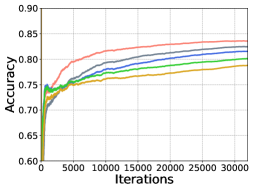
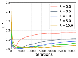
Figure 5: Ablations with different $\lambda$. We observe that increasing $\lambda$ results in lower accuracy and improved DP scores consistently throughout the online learning process.

Tree Ablations. In this experiment, we perform ablation experiments to investigate the impact of the number of trees in the oblique forest on the accuracy-fairness trade-off. In Figure 6, we report the change in average accuracy and demographic parity achieved during the online learning process in Adult dataset, when the number of trees in Aranyani is increased. We observe a slight decrease in accuracy (Figure 6 (left)) when the number of trees is increased, which can potentially result from overfitting. In a similar trend, we observe an improvement in the demographic parity (Figure 6 (right)), which is caused by the drop in accuracy due to overfitting.

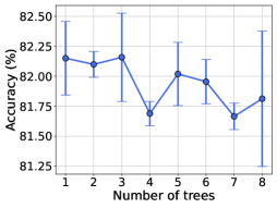
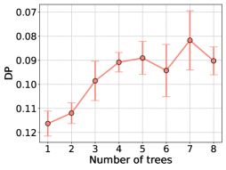
Figure 6: Ablation experiment with a varying number of trees, $|\mathcal{T}|$, in the oblique forest of Aranyani. We observe a slight drop in accuracy and a consistent drop in demographic parity when the number of trees used in Aranyani is increased.

Gradient Convergence. In this experiment, we investigate the convergence of fairness gradients (derived in Equation 5). We perform experiments on CivilComments dataset and report the gradient norms for all node parameters $(\mathbf{W},\mathbf{B})$ in Figure 7 (left & center). The $y$-axis in the figure is in log-scale for better visibility. We observe that the fairness gradients for both parameters converge over time and it is well correlated with the demographic parity of the decisions during online learning.

In Figure 7 (right), we study the gradient convergence bounds predicted by Theorem 2. Specifically, we try to understand how the fairness gradient norm varies as a function of the tree height. We observe a linear correlation between the magnitude of the fairness gradient norm and the height of the tree. However, in general, for small tree heights ($h\leq 10$), we observe that the gradient bound is quite slow and doesn’t impact the final demographic parity scores (which lie between $\sim$ 0.05-0.07).

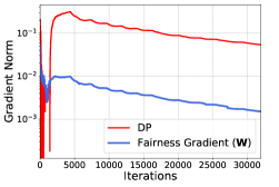
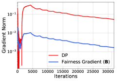
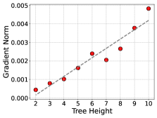
Figure 7: Convergence of gradients on CivilComments dataset: (left & center) We show the evolution of the gradient norms of the oblique tree parameters ($\mathbf{W},\mathbf{B}$) and the demographic parity during the online training process. We observe that the fairness gradients converge along with demographic parity. (right) We report the norm of the fairness gradients (for $\mathbf{W}$) at the end of online training with different tree heights. We observe that the gradient magnitude is very small and there appears to be a linear correlation with tree height.

References

- Abadi et al. (2015) Martín Abadi, Ashish Agarwal, Paul Barham, Eugene Brevdo, Zhifeng Chen, Craig Citro, Greg S. Corrado, Andy Davis, Jeffrey Dean, Matthieu Devin, Sanjay Ghemawat, Ian Goodfellow, Andrew Harp, Geoffrey Irving, Michael Isard, Yangqing Jia, Rafal Jozefowicz, Lukasz Kaiser, Manjunath Kudlur, Josh Levenberg, Dandelion Mané, Rajat Monga, Sherry Moore, Derek Murray, Chris Olah, Mike Schuster, Jonathon Shlens, Benoit Steiner, Ilya Sutskever, Kunal Talwar, Paul Tucker, Vincent Vanhoucke, Vijay Vasudevan, Fernanda Viégas, Oriol Vinyals, Pete Warden, Martin Wattenberg, Martin Wicke, Yuan Yu, and Xiaoqiang Zheng. TensorFlow: Large-scale machine learning on heterogeneous systems, 2015. URL https://www.tensorflow.org/. Software available from tensorflow.org.
- Agarwal et al. (2018) Alekh Agarwal, Alina Beygelzimer, Miroslav Dudík, John Langford, and Hanna Wallach. A reductions approach to fair classification. In International conference on machine learning, pp. 60–69. PMLR, 2018.
- Aghaei et al. (2019) Sina Aghaei, Mohammad Javad Azizi, and Phebe Vayanos. Learning optimal and fair decision trees for non-discriminative decision-making. In Proceedings of the AAAI conference on artificial intelligence, volume 33, pp. 1418–1426, 2019.
- Ajalloeian & Stich (2020) Ahmad Ajalloeian and Sebastian U Stich. On the convergence of sgd with biased gradients. arXiv preprint arXiv:2008.00051, 2020.
- Alghamdi et al. (2022) Wael Alghamdi, Hsiang Hsu, Haewon Jeong, Hao Wang, Peter Michalak, Shahab Asoodeh, and Flavio Calmon. Beyond adult and compas: Fair multi-class prediction via information projection. Advances in Neural Information Processing Systems, 35:38747–38760, 2022.
- Angwin et al. (2016) Julia Angwin, Jeff Larson, Surya Mattu, and Lauren Kirchner. Machine bias. In Ethics of data and analytics, pp. 254–264. Auerbach Publications, 2016.
- Baharlouei et al. (2020) Sina Baharlouei, Maher Nouiehed, Ahmad Beirami, and Meisam Razaviyayn. Rényi fair inference. In International Conference on Learning Representations, 2020.
- Barrett et al. (2019) Maria Barrett, Yova Kementchedjhieva, Yanai Elazar, Desmond Elliott, and Anders Søgaard. Adversarial removal of demographic attributes revisited. In Proceedings of the 2019 Conference on Empirical Methods in Natural Language Processing and the 9th International Joint Conference on Natural Language Processing (EMNLP-IJCNLP), pp. 6330–6335, 2019.
- Basu Roy Chowdhury et al. (2021) Somnath Basu Roy Chowdhury, Sayan Ghosh, Yiyuan Li, Junier Oliva, Shashank Srivastava, and Snigdha Chaturvedi. Adversarial scrubbing of demographic information for text classification. In Proceedings of the 2021 Conference on Empirical Methods in Natural Language Processing, pp. 550–562, Online and Punta Cana, Dominican Republic, November 2021. Association for Computational Linguistics. doi: 10.18653/v1/2021.emnlp-main.43. URL https://aclanthology.org/2021.emnlp-main.43.
- Bechavod et al. (2020) Yahav Bechavod, Christopher Jung, and Steven Z Wu. Metric-free individual fairness in online learning. Advances in neural information processing systems, 33:11214–11225, 2020.
- Becker & Kohavi (1996) Barry Becker and Ronny Kohavi. Adult. UCI Machine Learning Repository, 1996. DOI: https://doi.org/10.24432/C5XW20.
- Biewald (2020) Lukas Biewald. Experiment tracking with weights and biases, 2020. URL https://www.wandb.com/. Software available from wandb.com.
- Bifet & Gavalda (2009) Albert Bifet and Ricard Gavalda. Adaptive learning from evolving data streams. In Advances in Intelligent Data Analysis VIII: 8th International Symposium on Intelligent Data Analysis, IDA 2009, Lyon, France, August 31-September 2, 2009. Proceedings 8, pp. 249–260. Springer, 2009.
- Buolamwini & Gebru (2018) Joy Buolamwini and Timnit Gebru. Gender shades: Intersectional accuracy disparities in commercial gender classification. In Conference on fairness, accountability and transparency, pp. 77–91. PMLR, 2018.
- Calmon et al. (2017) Flavio Calmon, Dennis Wei, Bhanukiran Vinzamuri, Karthikeyan Natesan Ramamurthy, and Kush R Varshney. Optimized pre-processing for discrimination prevention. Advances in neural information processing systems, 30, 2017.
- Chami et al. (2020) Ines Chami, Albert Gu, Vaggos Chatziafratis, and Christopher Ré. From trees to continuous embeddings and back: Hyperbolic hierarchical clustering. Advances in Neural Information Processing Systems, 33:15065–15076, 2020.
- Chowdhury & Chaturvedi (2022) Somnath Basu Roy Chowdhury and Snigdha Chaturvedi. Learning fair representations via rate-distortion maximization. Transactions of the Association for Computational Linguistics, 10:1159–1174, 2022.
- Chowdhury & Chaturvedi (2023) Somnath Basu Roy Chowdhury and Snigdha Chaturvedi. Sustaining fairness via incremental learning. In Proceedings of the AAAI Conference on Artificial Intelligence, volume 37, pp. 6797–6805, 2023.
- Corbett-Davies et al. (2017) Sam Corbett-Davies, Emma Pierson, Avi Feller, Sharad Goel, and Aziz Huq. Algorithmic decision making and the cost of fairness. In Proceedings of the 23rd acm sigkdd international conference on knowledge discovery and data mining, pp. 797–806, 2017.
- Dastin (2022) Jeffrey Dastin. Amazon scraps secret ai recruiting tool that showed bias against women. In Ethics of data and analytics, pp. 296–299. Auerbach Publications, 2022.
- Do (2019) Quan Do. Jigsaw unintended bias in toxicity classification. 2019.
- Domingos & Hulten (2000) Pedro Domingos and Geoff Hulten. Mining high-speed data streams. In Proceedings of the sixth ACM SIGKDD international conference on Knowledge discovery and data mining, pp. 71–80, 2000.
- Drozdov et al. (2019) Andrew Drozdov, Pat Verga, Mohit Yadav, Mohit Iyyer, and Andrew McCallum. Unsupervised latent tree induction with deep inside-outside recursive autoencoders. arXiv preprint arXiv:1904.02142, 2019.
- Dua et al. (2017) Dheeru Dua, Casey Graff, et al. Uci machine learning repository. 2017.
- Dwork et al. (2012) Cynthia Dwork, Moritz Hardt, Toniann Pitassi, Omer Reingold, and Richard Zemel. Fairness through awareness. In Proceedings of the 3rd innovations in theoretical computer science conference, pp. 214–226, 2012.
- Gillen et al. (2018) Stephen Gillen, Christopher Jung, Michael Kearns, and Aaron Roth. Online learning with an unknown fairness metric. Advances in neural information processing systems, 31, 2018.
- Hardt et al. (2016) Moritz Hardt, Eric Price, and Nati Srebro. Equality of opportunity in supervised learning. Advances in neural information processing systems, 29, 2016.
- Hashimoto et al. (2018) Tatsunori Hashimoto, Megha Srivastava, Hongseok Namkoong, and Percy Liang. Fairness without demographics in repeated loss minimization. In International Conference on Machine Learning, pp. 1929–1938. PMLR, 2018.
- Hoeffding (1994) Wassily Hoeffding. Probability inequalities for sums of bounded random variables. The collected works of Wassily Hoeffding, pp. 409–426, 1994.
- Hort et al. (2022) Max Hort, Zhenpeng Chen, Jie M Zhang, Federica Sarro, and Mark Harman. Bias mitigation for machine learning classifiers: A comprehensive survey. arXiv preprint arXiv:2207.07068, 2022.
- Huber (1992) Peter J Huber. Robust estimation of a location parameter. In Breakthroughs in statistics: Methodology and distribution, pp. 492–518. Springer, 1992.
- Jasinska-Kobus et al. (2021) Kalina Jasinska-Kobus, Marek Wydmuch, Devanathan Thiruvenkatachari, and Krzysztof Dembczynski. Online probabilistic label trees. In International Conference on Artificial Intelligence and Statistics, pp. 1801–1809. PMLR, 2021.
- Jernite et al. (2016) Yacine Jernite, Anna Choromanska, David Sontag, and Yann LeCun. Simultaneous learning of trees and representations for extreme classification, with application to language modeling. arXiv preprint arXiv:1610.04658, 2016.
- Jordan & Jacobs (1994) Michael I Jordan and Robert A Jacobs. Hierarchical mixtures of experts and the em algorithm. Neural computation, 6(2):181–214, 1994.
- Jung et al. (2022a) Sangwon Jung, Sanghyuk Chun, and Taesup Moon. Learning fair classifiers with partially annotated group labels. In Proceedings of the IEEE/CVF Conference on Computer Vision and Pattern Recognition, pp. 10348–10357, 2022a.
- Jung et al. (2022b) Sangwon Jung, Taeeon Park, Sanghyuk Chun, and Taesup Moon. Re-weighting based group fairness regularization via classwise robust optimization. In The Eleventh International Conference on Learning Representations, 2022b.
- Kamiran et al. (2010) Faisal Kamiran, Toon Calders, and Mykola Pechenizkiy. Discrimination aware decision tree learning. In 2010 IEEE international conference on data mining, pp. 869–874. IEEE, 2010.
- Karthikeyan et al. (2022) Ajaykrishna Karthikeyan, Naman Jain, Nagarajan Natarajan, and Prateek Jain. Learning accurate decision trees with bandit feedback via quantized gradient descent. Transactions on Machine Learning Research, 2022.
- Kingma & Ba (2014) Diederik P Kingma and Jimmy Ba. Adam: A method for stochastic optimization. arXiv preprint arXiv:1412.6980, 2014.
- Kirkpatrick et al. (2017) James Kirkpatrick, Razvan Pascanu, Neil Rabinowitz, Joel Veness, Guillaume Desjardins, Andrei A Rusu, Kieran Milan, John Quan, Tiago Ramalho, Agnieszka Grabska-Barwinska, et al. Overcoming catastrophic forgetting in neural networks. Proceedings of the national academy of sciences, 114(13):3521–3526, 2017.
- Konečnỳ et al. (2016) Jakub Konečnỳ, H Brendan McMahan, Felix X Yu, Peter Richtárik, Ananda Theertha Suresh, and Dave Bacon. Federated learning: Strategies for improving communication efficiency. arXiv preprint arXiv:1610.05492, 2016.
- Lahoti et al. (2020) Preethi Lahoti, Alex Beutel, Jilin Chen, Kang Lee, Flavien Prost, Nithum Thain, Xuezhi Wang, and Ed Chi. Fairness without demographics through adversarially reweighted learning. Advances in neural information processing systems, 33:728–740, 2020.
- Larson et al. (2016) Jeff Larson, Surya Mattu, Lauren Kirchner, and Julia Angwin. How we analyzed the compas recidivism algorithm. ProPublica (5 2016), 9(1):3–3, 2016.
- Liu et al. (2021) Evan Z Liu, Behzad Haghgoo, Annie S Chen, Aditi Raghunathan, Pang Wei Koh, Shiori Sagawa, Percy Liang, and Chelsea Finn. Just train twice: Improving group robustness without training group information. In International Conference on Machine Learning, pp. 6781–6792. PMLR, 2021.
- Liu et al. (2015) Ziwei Liu, Ping Luo, Xiaogang Wang, and Xiaoou Tang. Deep learning face attributes in the wild. In Proceedings of International Conference on Computer Vision (ICCV), December 2015.
- Lowy et al. (2022) Andrew Lowy, Sina Baharlouei, Rakesh Pavan, Meisam Razaviyayn, and Ahmad Beirami. A stochastic optimization framework for fair risk minimization. Transactions on Machine Learning Research, 2022.
- Macaulay & Fourment (2023) Matthew Macaulay and Mathieu Fourment. Differentiable phylogenetics via hyperbolic embeddings with dodonaphy. arXiv preprint arXiv:2309.11732, 2023.
- Mary et al. (2019) Jérémie Mary, Clément Calauzenes, and Noureddine El Karoui. Fairness-aware learning for continuous attributes and treatments. In International Conference on Machine Learning, pp. 4382–4391. PMLR, 2019.
- Mehrabi et al. (2021) Ninareh Mehrabi, Fred Morstatter, Nripsuta Saxena, Kristina Lerman, and Aram Galstyan. A survey on bias and fairness in machine learning. ACM computing surveys (CSUR), 54(6):1–35, 2021.
- Mishler & Dalmasso (2022) Alan Mishler and Niccolò Dalmasso. Fair when trained, unfair when deployed: Observable fairness measures are unstable in performative prediction settings. arXiv preprint arXiv:2202.05049, 2022.
- Monath et al. (2017) Nicholas Monath, Ari Kobren, Akshay Krishnamurthy, and Andrew McCallum. Gradient-based hierarchical clustering. In 31st Conference on neural information processing systems (NIPS 2017), Long Beach, CA, USA, volume 1, pp. 6, 2017.
- Monath et al. (2019) Nicholas Monath, Manzil Zaheer, Daniel Silva, Andrew McCallum, and Amr Ahmed. Gradient-based hierarchical clustering using continuous representations of trees in hyperbolic space. In Proceedings of the 25th ACM SIGKDD International Conference on Knowledge Discovery & Data Mining, pp. 714–722, 2019.
- Murthy et al. (1994) Sreerama K Murthy, Simon Kasif, and Steven Salzberg. A system for induction of oblique decision trees. Journal of artificial intelligence research, 2:1–32, 1994.
- Nagano et al. (2019) Yoshihiro Nagano, Shoichiro Yamaguchi, Yasuhiro Fujita, and Masanori Koyama. A wrapped normal distribution on hyperbolic space for gradient-based learning. In International Conference on Machine Learning, pp. 4693–4702. PMLR, 2019.
- Penn et al. (2023) Matthew J Penn, Neil Scheidwasser, Joseph Penn, Christl A Donnelly, David A Duchêne, and Samir Bhatt. Leaping through tree space: continuous phylogenetic inference for rooted and unrooted trees. arXiv preprint arXiv:2306.05739, 2023.
- Pleiss et al. (2017) Geoff Pleiss, Manish Raghavan, Felix Wu, Jon Kleinberg, and Kilian Q Weinberger. On fairness and calibration. Advances in neural information processing systems, 30, 2017.
- Prost et al. (2019) Flavien Prost, Hai Qian, Qiuwen Chen, Ed H Chi, Jilin Chen, and Alex Beutel. Toward a better trade-off between performance and fairness with kernel-based distribution matching. arXiv preprint arXiv:1910.11779, 2019.
- Qiao & Peng (2022) Fengchun Qiao and Xi Peng. Graph-relational distributionally robust optimization. In NeurIPS 2022 Workshop on Distribution Shifts: Connecting Methods and Applications, 2022.
- Quadrianto & Sharmanska (2017) Novi Quadrianto and Viktoriia Sharmanska. Recycling privileged learning and distribution matching for fairness. Advances in neural information processing systems, 30, 2017.
- Radford et al. (2021) Alec Radford, Jong Wook Kim, Chris Hallacy, Aditya Ramesh, Gabriel Goh, Sandhini Agarwal, Girish Sastry, Amanda Askell, Pamela Mishkin, Jack Clark, et al. Learning transferable visual models from natural language supervision. In International conference on machine learning, pp. 8748–8763. PMLR, 2021.
- Raff et al. (2018) Edward Raff, Jared Sylvester, and Steven Mills. Fair forests: Regularized tree induction to minimize model bias. In Proceedings of the 2018 AAAI/ACM Conference on AI, Ethics, and Society, pp. 243–250, 2018.
- Raji & Buolamwini (2019) Inioluwa Deborah Raji and Joy Buolamwini. Actionable auditing: Investigating the impact of publicly naming biased performance results of commercial ai products. In Proceedings of the 2019 AAAI/ACM Conference on AI, Ethics, and Society, pp. 429–435, 2019.
- Rezaei et al. (2021) Ashkan Rezaei, Anqi Liu, Omid Memarrast, and Brian D Ziebart. Robust fairness under covariate shift. In Proceedings of the AAAI Conference on Artificial Intelligence, volume 35, pp. 9419–9427, 2021.
- Rusu et al. (2016) Andrei A Rusu, Neil C Rabinowitz, Guillaume Desjardins, Hubert Soyer, James Kirkpatrick, Koray Kavukcuoglu, Razvan Pascanu, and Raia Hadsell. Progressive neural networks. arXiv preprint arXiv:1606.04671, 2016.
- Shin et al. (2016) Richard Shin, Alexander A Alemi, Geoffrey Irving, and Oriol Vinyals. Tree-structured variational autoencoder. 2016.
- Su et al. (2022) Hongjin Su, Weijia Shi, Jungo Kasai, Yizhong Wang, Yushi Hu, Mari Ostendorf, Wen-tau Yih, Noah A. Smith, Luke Zettlemoyer, and Tao Yu. One embedder, any task: Instruction-finetuned text embeddings. 2022. URL https://arxiv.org/abs/2212.09741.
- Sun et al. (2019) Wen Sun, Alina Beygelzimer, Hal Daumé Iii, John Langford, and Paul Mineiro. Contextual memory trees. In International Conference on Machine Learning, pp. 6026–6035. PMLR, 2019.
- Voigt & Von dem Bussche (2017) Paul Voigt and Axel Von dem Bussche. The eu general data protection regulation (gdpr). A Practical Guide, 1st Ed., Cham: Springer International Publishing, 10(3152676):10–5555, 2017.
- Wang et al. (2023) Haotao Wang, Junyuan Hong, Jiayu Zhou, and Zhangyang Wang. How robust is your fairness? evaluating and sustaining fairness under unseen distribution shifts. Transactions on machine learning research, 2023, 2023.
- Wolf et al. (2019) Thomas Wolf, Lysandre Debut, Victor Sanh, Julien Chaumond, Clement Delangue, Anthony Moi, Pierric Cistac, Tim Rault, Rémi Louf, Morgan Funtowicz, et al. Huggingface’s transformers: State-of-the-art natural language processing. arXiv preprint arXiv:1910.03771, 2019.
- Yang et al. (2019) Zhilin Yang, Thang Luong, Russ R Salakhutdinov, and Quoc V Le. Mixtape: Breaking the softmax bottleneck efficiently. Advances in Neural Information Processing Systems, 32, 2019.
- Yin et al. (2018) Pengcheng Yin, Chunting Zhou, Junxian He, and Graham Neubig. StructVAE: Tree-structured latent variable models for semi-supervised semantic parsing. In Proceedings of the 56th Annual Meeting of the Association for Computational Linguistics (Volume 1: Long Papers), pp. 754–765, Melbourne, Australia, July 2018. Association for Computational Linguistics. doi: 10.18653/v1/P18-1070. URL https://aclanthology.org/P18-1070.
- Yu et al. (2022) Hsiang-Fu Yu, Kai Zhong, Jiong Zhang, Wei-Cheng Chang, and Inderjit S Dhillon. Pecos: Prediction for enormous and correlated output spaces. the Journal of machine Learning research, 23(1):4233–4264, 2022.
- Zemel et al. (2013) Rich Zemel, Yu Wu, Kevin Swersky, Toni Pitassi, and Cynthia Dwork. Learning fair representations. In International conference on machine learning, pp. 325–333. PMLR, 2013.
- Zhang & Ntoutsi (2019) Wenbin Zhang and Eirini Ntoutsi. Faht: An adaptive fairness-aware decision tree classifier. 2019.
- Zhao et al. (2023) Chen Zhao, Feng Mi, Xintao Wu, Kai Jiang, Latifur Khan, Christan Grant, and Feng Chen. Towards fair disentangled online learning for changing environments. In Proceedings of the 29th ACM SIGKDD Conference on Knowledge Discovery and Data Mining, pp. 3480–3491, 2023.
- Zhao et al. (2020) Jinyu Zhao, Yi Hao, and Cyrus Rashtchian. Unsupervised embedding of hierarchical structure in euclidean space. arXiv preprint arXiv:2010.16055, 2020.