Gaia FGK Benchmark Stars: fundamental $T_{\rm eff}$ and $\log g$ of the third version

Abstract

Context. Large spectroscopic surveys devoted to the study of the Milky Way, including Gaia, use automated pipelines to massively determine the atmospheric parameters of millions of stars. The Gaia FGK Benchmark Stars are reference stars with $T_{\rm eff}$ and $\log g$ derived through fundamental relations, independently of spectroscopy, to be used as anchors for the parameter scale. The first and second versions of the sample have been extensively used for that purpose, and more generally to help constrain stellar models.

Aims. We provide the third version of the Gaia FGK Benchmark Stars, an extended set intended to improve the calibration of spectroscopic surveys, and their interconnection.

Methods. We have compiled about 200 candidates which have precise measurements of angular diameters and parallaxes. We determined their bolometric fluxes by fitting their spectral energy distribution. Masses were determined using two sets of stellar evolution models. In a companion paper we describe the determination of metallicities and detailed abundances.

Results. We provide a new set of 192 Gaia FGK Benchmark Stars with their fundamental $T_{\rm eff}$ and $\log g$, and with uncertainties lower than 2% for most stars. Compared to the previous versions, the homogeneity and accuracy of the fundamental parameters are significantly improved thanks to the high quality of the Gaia photometric and astrometric data.

1 Introduction

The last decade has been marked by a large observational effort aimed at deciphering the history of our Galaxy based on large samples of stars observed by spectroscopic surveys. This has stimulated the development of efficient methodologies for the massive determination of atmospheric parameters (APs). In particular the recent Gaia Data Release 3 (Gaia Collaboration et al., 2023c, Gaia DR3) just delivered $T_{\rm eff}$, $\log g$ and [Fe/H] for millions of stars (Creevey et al., 2023; Fouesneau et al., 2023). In particular two datasets were released that mainly include F, G and K-type stars, one for 5.6 million stars with APs based on medium resolution spectra from the Radial Velocity Spectrometer (Recio-Blanco et al., 2023), the other one for 471 million stars with APs based on low resolution spectra from the blue and red prisms, parallax and integrated photometry (Andrae et al., 2023). The methodologies used for the massive determination of atmospheric parameters rely on stellar models which are not perfect and not able to reproduce exactly real spectra, causing some biases which have to be corrected.

The Gaia FGK Benchmark Stars (GBS) are reference stars to be used for the calibration and the validation of spectroscopic methods of parametrisation. They are chosen to cover the range of F, G, and K spectral types at different luminosities and metallicities, and to have the necessary observations available to determine their effective temperature and surface gravity independently from spectroscopy, at a precision level of 1-2%. The determination of $T_{\rm eff}$ and $\log g$  is performed through the fundamental relations implying observable quantities (angular diameters directly measured by interferometry, bolometric fluxes and parallaxes) and the mass, the only parameter depending on theoretical assumptions.

The first and second versions of the GBS (hereafter V1 and V2, respectively) were presented in a series of papers. Heiter et al. (2015), hereafter Paper I, describe the initial selection of 34 stars, including the Sun, and the determination of their fundamental effective temperatures and surface gravities, resulting in the GBS V1 sample. Blanco-Cuaresma et al. (2014) (Paper II) present the library of high-resolution spectra that was assembled and used to determine metallicities (Jofré et al., 2014, Paper III) and elemental abundances of $\alpha-$capture and iron-peak elements (Jofré et al., 2015, Paper IV). One limitation of the V1 sample was the small number of targets, in particular in the metal-poor regime. Metal-poor stars are usually distant and faint, which makes them difficult to observe in interferometry. In Paper V, Hawkins et al. (2016) proposed a list of ten metal-poor stars to be included in the GBS sample. The GBS V2 sample summarised by Jofré et al. (2018) includes 36 stars, merged from Paper I and Paper V. The change in number from 34 to 36 comes from the addition of five metal-poor stars from Paper V and the removal of some stars from Paper I because their spectroscopic analysis indicated that they could not be recommended as reference stars. However, V2 was an intermediate version where the fundamental properties of the stars were not redetermined owing to the lack of direct and accurate measurements of angular diameters for some stars.

The material provided in these series of papers consists of accurate APs for stars covering a extensive range of spectral types and metallicities, in addition to a library of high resolution and high signal-to-noise spectra from which line-by-line abundances are also provided. This material can be further exploited in spectroscopic studies. Indeed, Paper VI of the GBS series (Jofré et al., 2017), reports on a collective work using the GBS to investigate the different sources of uncertainties in elemental abundances in order to improve spectroscopic pipelines.

The ultimate goal of the efforts dealing with GBS is to provide to spectroscopic surveys the fundamental $T_{\rm eff}$ and $\log g$ scales and an external reference for abundances. Despite their limitation in sample size and parallax precision previous to Gaia data, the GBS have been extensively used in the past years. The Gaia astrophysical parameters inference system (Bailer-Jones et al., 2013; Creevey et al., 2023) made use of GBS for the validation of the stellar parameters published in Gaia DR3. The GBS are also a fundamental source of calibration and validation of the Gaia-ESO Survey (Gilmore et al., 2022; Randich et al., 2022; Hourihane et al., 2023), of the RAVE survey (Steinmetz et al., 2020b, a), and of the GALAH survey (Buder et al., 2021). The OCCASO project (Casamiquela et al., 2019) has systematically observed two GBS giants, Arcturus and $\mu$ Leo, to validate chemical abundances of open clusters. Upcoming large projects such as WEAVE (Jin et al., 2022) are also making use of the GBS.

Calibrations based on GBS can help to make surveys more homogeneous and mutually compatible so that they can be combined into the most comprehensive database of chemical measurements for the study of the Milky Way stellar populations (Jofré et al., 2018). The applications of the GBS however can extend far beyond this specific purpose. As for the study presented in Paper VI (see also Blanco-Cuaresma, 2019), many spectroscopic studies have benefited from the GBS effort. For example, Adibekyan et al. (2020) used the GBS to assess the performances of the ESPRESSO, PEPSI and HARPS high-resolution spectrographs while Heiter et al. (2021) used some spectra from Paper II to assess the quality of hundreds of spectral lines and the corresponding atomic and molecular data used for the abundance analyses of FGK-type stars carried out within the Gaia-ESO survey (see also Kondo et al., 2019; Fukue et al., 2021, for lines in the Infrared). Amarsi et al. (2022) and Lind et al. (2022) used the GBS to quantify the differences in abundances derived using state-of-the-art 3D non-LTE atmosphere models and the standard 1D LTE models.

In addition to spectroscopy, the GBS help to constrain better stellar evolution models. For example, Sahlholdt et al. (2019) determined ages of the GBS as a way to test the reliability of the determination of stellar ages for various stellar populations; Serenelli et al. (2017) used GBS to validate their asteroseismic analysis performed on dwarfs and subgiants. The GBS have also been used as validation for the PLATO stellar analysis pipeline (Gent et al., 2022). Many of the lessons learnt from the GBS are further discussed in Jofré et al. (2019).

However, we are aware that the current sample of GBS is still imperfect and too small to make a satisfactory interconnection between surveys. This is why an extension of the sample is required. The V1 and V2 GBS samples were also limited by the parallax accuracy needed for a fundamental $\log g$ determination. This is not anymore an issue thanks to the exquisite astrometric quality of the Gaia data (Gaia Collaboration et al., 2016).

In this Paper VII of the series, we present the extended sample and third version of the GBS (GBS V3) that includes about 200 stars. We took advantage of recent interferometric studies that provided new measurements of angular diameters for large samples of stars (e.g. Ligi et al., 2016; Baines et al., 2018, 2021; van Belle et al., 2021) and for metal-poor stars (e.g. Creevey et al., 2015; Karovicova et al., 2018, 2020). As explained in Sect. 2 we selected new GBS candidates based on quality criteria applied on interferometric measurements. Sect. 3 describes the compilation of angular diameters and fluxes that are needed to compute the fundamental $T_{\rm eff}$. Bolometric fluxes ($F_{\rm bol}$) were homogeneously computed by the method of spectral energy distribution (SED) fitting based on a large collection of (spectro)photometric data. Sect. 4 deals with the determination of $\log g$ with parallaxes from Gaia DR3 (Gaia Collaboration et al., 2023c), or Hipparcos (van Leeuwen, 2007) for the brightest stars, and with masses inferred from a state-of-the-art methodology and stellar tracks. At each of these different steps we assess the uncertainties of the stellar parameters. Sect. 5 provides an overview of the sample properties and shows some comparisons to $T_{\rm eff}$ and $\log g$ from different catalogues, before our concluding remarks in Sect. 6. All the compiled and computed parameters of this work are given in the form of a catalogue distributed by the CDS. We note that these parameters still require a last iteration considering [Fe/H] values, needed for the estimation of $F_{\rm bol}$ and masses and here adopted from the literature, that are consistent with our fundamental parameters. This is a necessary step to recommend our parameters for reference (Heiter et al., 2015). The accompanying Paper VIII (Casamiquela et al. in preparation) presents homogeneous determinations of [Fe/H] and of detailed abundances of the GBS V3 derived from a spectroscopic analysis. For this purpose a large dataset of high-resolution, high signal-to-noise spectra was collected from public archives and through our own observing programs. The recommended parameters and abundances of the GBS are appropriately updated at the CDS.

2 Star selection

In order to determine $T_{\rm eff}$ and $\log g$ through the fundamental relations with a minimum of assumptions and theoretical input, our principal criterion was to choose F, G and K stars with a high quality measurement of angular diameter. Ideally we want our GBS sample to homogeneously cover the ($T_{\rm eff}$,$\log g$,[Fe/H]) space, which implies a special effort to add metal-poor stars. We have therefore searched the literature for GBS candidates fulfilling these criteria.

First, we considered the GBS from V1 and V2 (Heiter et al., 2015; Jofré et al., 2018). The GBS V1 sample has 29 FGK-type stars (including the Sun), four giants with $T_{\rm eff}$ around 4000 K, corresponding to late K and early M spectral types, and one cooler M giant. The V2 sample was built from the V1 one, with the addition of metal-poor stars. For the V3 list we considered all the 39 V1 and V2 stars including several stars with indirect determinations of angular diameters. For all we searched for new direct determinations of angular diameters as well as other data needed to update their fundamental $T_{\rm eff}$ and $\log g$. We added to this list eight metal-poor stars from Karovicova et al. (2020, 2022a), not part of V1 and V2, and two targets recently observed with the CHARA interferometer (Creevey et al. in preparation). This sample of 49 stars was our initial set.

To further extend the GBS sample, we searched for new candidates observed in interferometry. We used the compilation from the Jean-Marie Mariotti Center (JMMC), the JMMC Measured Stellar Diameters Catalogue (JMDC, Duvert, 2016). This catalogue, regularly updated, intends to be as exhaustive as possible in listing all the measurements of stellar apparent diameters made with direct techniques. It is therefore a very appropriate resource to extend the GBS sample. The JMDC is a bibliographical catalogue which implies that some stars have multiple entries, resulting from studies with different instruments, in different bands and with different precisions. Deciding which value of angular diameter is the most appropriate for a given star can be challenging, in particular owing to non-homogeneous uncertainties listed in the JMDC. In addition, there are many stars in the JMDC which are not appropriate for our purpose, such as some classes of variable stars, hot stars, spectroscopic binaries, and fast rotators. In addition, some very uncertain measurements of angular diameters could propagate large uncertainties to $T_{\rm eff}$ and should be discarded. Therefore we made a first selection to reject stars and measurements not relevant for our purpose.

To do so, we followed Salsi et al. (2020) who established accurate surface brightness-colour relations for different spectral types and luminosity classes. They applied three types of rejection criteria on the JMDC data. First they examined the stellar characteristics to reject variable and semi-regular pulsating stars, spectroscopic binaries and other multiple stars, fast rotators and stars with a doubtful luminosity class. Second, they used criteria on the quality of the interferometric measurements that we apply similarly (see Sect. 3.1). The third type of criterion is based on the uncertainty of the K magnitude. We considered their list of 106 carefully selected F5 to K7 dwarfs and giants that we added to the initial set (five stars were already there). However, the study of Salsi et al. (2020) does not take into account the metallicity of the stars since their objective is to infer radii of stars and planets in the context of the PLATO mission which mainly focuses on solar-like stars. For us the metallicity is essential since the GBS should be representative of all the Milky Way stellar populations. We aim to improve the sampling of the GBS in $T_{\rm eff}$ and $\log g$ but also in [Fe/H] with as many GBS candidates as possible on the metal-poor side. We noticed that the criteria used by Salsi et al. (2020), in particular the photometric one, tend to reject metal-poor stars. The only star with [Fe/H]$<-$1.0 in Salsi et al. (2020)’s sample is the well-known benchmark star HIP76976 (HD 140283), part of GBS V1, which has [Fe/H]=$-$2.36$\pm$0.10 in Paper IV.

We then searched for additional stars in the September 2021 version of JMDC available at the CDS which includes 2013 measurements of 1062 stars, a significant increase compared to the February 2020 version used by Salsi et al. (2020). In order to find stars in the appropriate range of atmospheric parameters, we used the PASTEL catalogue (Soubiran et al., 2016) and its recent version which provides mean atmospheric parameters for 14 181 FGK stars (Soubiran et al., 2022). We expect PASTEL to be complete for metal-poor stars brighter than V$\sim$8.25, which is the limiting magnitude of FGK-type stars with an interferometric measurement in JMDC. Among the $\sim$500 stars in common between PASTEL and JMDC, we considered 63 additional stars to include in our sample, because they fill gaps in the AP space, and their interferometric angular diameters fulfill the criteria of Salsi et al. (2020).

The resulting list of selected candidates for GBS V3 includes 201 stars (the Sun is not considered here) They are all members of the Hipparcos catalogue (ESA 1997) and only the ten brightest ones are missing in Gaia DR3 (Gaia Collaboration et al., 2016). We keep the Sun in the GBS V3 since it is an obvious benchmark star, although it is not observable in the same conditions as other stars. We do not discuss the Sun in the present paper, keeping its fundamental $T_{\rm eff}$ and $\log g$ determined in Paper I (we also note that a nominal value for the effective temperature of the Sun was adopted at the XXIXth IAU General Assembly, see Mamajek et al. 2015; Prša et al. 2016).

In the following, metallicities [Fe/H] are needed for the determination of $F_{\rm bol}$ from SEDs (to initialize the minimization process, see Sect. 3.4), and for the determination of masses from stellar evolutionary tracks (see Sect. 4.2). We have adopted [Fe/H] from the literature for the 201 stars, mainly from the PASTEL catalogue. For a sake of homogeneity, we have not adopted [Fe/H] from Papers III and V for stars in V1 and V2 because they are corrected from non-local thermodynamic equilibrium (NLTE) effects, while for all the other stars the literature values are assuming LTE. It is the purpose of the forthcoming Paper VIII to provide precise and homogeneous abundances of Fe and other elements. This will imply some iterations to get the recommended $T_{\rm eff}$ and $\log g$ of our targets.

3 Fundamental effective temperature

The luminosity $L$, the radius $R$, and the effective temperature $T_{\rm eff}$ of a given star are linked through the fundamental relation $L=4\pi R^{2}\sigma T_{\rm eff}^{4}$, where $\sigma$ is the Stefan-Boltzmann constant. The fundamental relation can be expressed in a way that gives $T_{\rm eff}$ as a function of the limb-darkened angular diameter $\theta_{\rm LD}$ and the bolometric flux $F_{\rm bol}$ which are measurable quantities:

$$\centering T_{\rm eff}=\left(\frac{F_{\rm bol}}{\sigma}\right)^{0.25}(0.5\,\theta_{\rm LD})^{-0.5}=2341\left(\frac{F_{\rm bol}}{\theta_{\rm LD}^{2}}\right)^{0.25}\@add@centering$$ (1)

where $\theta_{\rm LD}$ is in milliarcseconds (mas) and $F_{\rm bol}$  in $10^{-8}$ erg s^-1 cm^-2 or $10^{-11}$ W m^-2.

In the following subsections we describe our compilation of measured angular diameters and fluxes. The latter were used to compute $F_{\rm bol}$ by means of SED fitting. Subsequently, Eq. (1) was used to obtain $T_{\rm eff}$ for the selected stars.

3.1 Compilation of angular diameters

As explained in Sect. 2, the selection of GBS V3 stars was mainly based on the JMDC which provides one or several values of $\theta_{\rm LD}$ for each star. In particular, we considered the 106 targets that Salsi et al. (2020) used as calibration stars to define precise surface brightness–colour relations. Salsi et al. (2020) applied interferometric criteria to remove non reliable values of $\theta_{\rm LD}$ in the JMDC. They rejected measurements with a relative uncertainty on the angular diameter larger than 8%, and those based on observations in the 8-13 micron band or having a bad observation quality and/or a poor spatial frequency coverage in the visibility curve. They also rejected stars with inconsistent redundancies. We adopted their selected values of $\theta_{\rm LD}$ for the 106 stars. For HIP112748 and HIP54539, provided with two values of $\theta_{\rm LD}$ differing by less than 1%, we adopted the one with the lowest uncertainty.

For the remaining stars, we queried JMDC and the recent literature in order to retrieve the latest values of $\theta_{\rm LD}$ fulfilling the interferometric criteria applied by Salsi et al. (2020). When provided we inspected the visibility curves to evaluate the reliability of the measurement.

We found recent and precise $\theta_{\rm LD}$ for ten of the GBS V1 and V2. In particular, for three of the metal-poor benchmark stars new measurements are available, for HD103095 (HIP57939) and HD122563 (HIP68594) by Karovicova et al. (2020), and for HD140283 (HIP76976) by Karovicova et al. (2018). The two components of the binary $\alpha$ Cen were remeasured by Kervella et al. (2017), while four other targets were found in Baines et al. (2018, 2021). Among the six stars which had no direct $\theta_{\rm LD}$ in Paper I, only one (HIP48455, $\mu$ Leo) was observed in interferometry by Baines et al. (2018). Among the five metal-poor stars from Paper V with indirect values of $\theta_{\rm LD}$, one (HIP92167) was observed by Karovicova et al. (2020). Thus, we are left with nine stars from V1 and V2 that are still without any direct measurement of $\theta_{\rm LD}$. We keep them in a separate table for continuity of the samples, but we do not consider them as GBS anymore.

The final version of the GBS V3 includes 192 stars with a direct measurement of $\theta_{\rm LD}$. For each we provide the limb darkened angular diameter with its uncertainty and the corresponding reference in Table LABEL:t:fund_teff_logg of Appendix A and in the catalogue available at the CDS. The sample includes stars with small angular diameters such as HIP97527 ($\theta_{\rm LD}$=0.231$\pm$0.006 mas) and HIP93427 ($\theta_{\rm LD}$=0.289$\pm$0.006 mas), both of which are asteroseismic targets observed with the CHARA/PAVO instrument by Huber et al. (2012). The sample also includes Aldebaran (HIP21421) and Arcturus (HIP69673) which have angular diameters as large as $\sim$20 mas. The median angular diameter of the sample is 1.12 mas.

The relative $\theta_{\rm LD}$ uncertainties range from 0.1% (HIP87808) to 7% (HIP25993) with a median value of 1.1% (see histogram in Fig. 1). Two other stars have relative uncertainties larger than 5%, HIP7294 and HIP14838. In absolute values, the largest uncertainties occur for the two giants $\psi$ Phe (HIP8837) and Arcturus (HIP69673), with $\theta_{\rm LD}$=8.0$\pm$0.2 mas and $\theta_{\rm LD}$=21.0$\pm$0.21 mas, respectively. The two stars do not seem to have been re-observed recently, so that their $\theta_{\rm LD}$ is still that of Paper I.

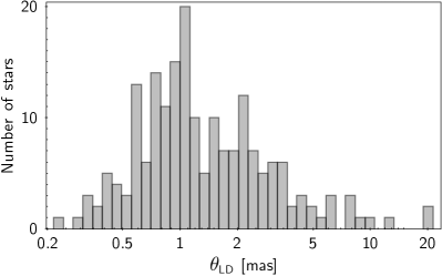
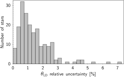
Figure 1: Histogram of $\theta_{\rm LD}$ (top panel) and its relative uncertainty (bottom panel) for the 192 GBS V3 stars having interferometric measurements.

We note that, for a small fraction of stars, we had to make a choice between the two or more values of $\theta_{\rm LD}$ fulfilling the adopted quality criteria. As shown in Fig. 2, several small diameters (typically $\theta_{\rm LD}$$<$1.5 mas) disagree by more than 10%, but in general the agreement is at the 2$\sigma$ level. We note three stars with estimations of their angular diameters differing by more than 3$\sigma$: HIP96441, HIP57939, HIP108870.

HIP96441 has three values of $\theta_{\rm LD}$ reported in the JMDC, that fulfill the interferometric criteria of Salsi et al. (2020): 0.861$\pm$0.015 mas in the K band (Boyajian et al., 2012a), 0.753$\pm$0.009 mas in the R band (White et al., 2013) and 0.749$\pm$0.007 mas in the H band (Ligi et al., 2016). The first determination is not compatible with the two others, but Boyajian et al. (2013) mention a calibration problem and discarded this star. Between the two other values we adopted the most recent one by Ligi et al. (2016).

HIP57939 (HD103095) is a well-known metal-poor dwarf studied by several authors. We adopted the latest determination, $\theta_{\rm LD}$=0.593$\pm$0.004 mas, by Karovicova et al. (2020) who used the combination of two instruments, VEGA and PAVO on the CHARA interferometer giving a high confidence to their result.

For HIP108870 we adopted the value $\theta_{\rm LD}$=1.758$\pm$0.012 mas by Rains et al. (2020) which significantly differs from that previously reported by Kervella et al. (2004), $\theta_{\rm LD}$=1.89$\pm$0.02 mas. Rains et al. (2020) have analysed this discrepancy, considering that they obtained tighter constraints on the angular diameter by better resolving the star, thanks to the configuration now available at the VLTI.

These cases of disagreement also illustrate the inhomogeneity of uncertainties listed in JMDC, which sometimes only reflect the precision of a fit, or also include systematic effects identified at the calibration level. The dispersion among measurements available for a given star is critical for small angular diameters, typically below $\sim$1.5 mas, because it corresponds to discrepancies that can reach 10 to 15%. This illustrates the limitations of measuring interferometric diameters in the sub-mas regime. Some inhomogeneity can also arise from different recipes applied for the limb darkening correction. According to Eq. (1), a variation of 10% in $\theta_{\rm LD}$ translates into a variation of 5% in $T_{\rm eff}$. Inversely, a 1% precision on $T_{\rm eff}$ implies angular diameters obtained at the 2% level.

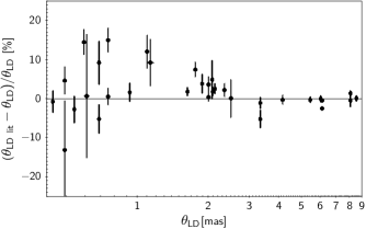
Figure 2: Difference between $\theta_{\rm LD}$ adopted for this work and other values in JMDC fulfilling the selection criteria by Salsi et al. (2020).

3.2 Compilation of magnitudes and fluxes

In order to build a SED for each star and measure the corresponding $F_{\rm bol}$ we compiled fluxes using the VOSA tool (Bayo et al., 2008). VOSA allowed us to collect all the photometry available in the Virtual Observatory (VO) for our list of 201 stars (including the nine stars from V1 and V2 with an indirect $\theta_{\rm LD}$) and to convert magnitudes into fluxes thanks to an exhaustive description of all the existing filters. We only kept the photometry from the VO catalogues that contain at least fifty of our targets, namely 2MASS (Cutri et al., 2003), AKARI (Yamamura et al., 2010), Gaia DR3 (Gaia Collaboration et al., 2023c), GALEX (Bianchi et al., 2017), Strömgren photometric catalogues (Hauck & Mermilliod, 1998; Paunzen, 2015), Johnson UBV (Mermilliod, 1987), IRAS (Neugebauer et al., 1984), Hipparcos (ESA, 1997), Tycho-2 (Høg et al., 2000) and WISE (Cutri et al., 2021).

We note that the components of the bright binary star $\alpha$ Cen A and B are not resolved in the 2MASS catalog, and the magnitudes given for $\alpha$ Cen A contain actually the combined flux of both components. We therefore used J, H, and K magnitudes from Engels et al. (1981), which are given for each component separately, and converted them to flux values using the VOSA tool.

An interesting new feature of the latest VOSA version (July 2022 update) is to provide synthetic photometry based on Gaia DR3 BP/RP spectra analysed with the GaiaXPy tool (De Angeli et al., 2023; Gaia Collaboration et al., 2023b). We therefore collected through VOSA the synthetic photometry from Gaia which is provided in 13 passbands corresponding to the filters of the Hubble Space Telescope, Sloan Digital Sky Survey, PanSTARRS1 and Johnson UBVRI systems. Also from Gaia BP/RP spectra and GaiaXPy, VOSA computes fluxes in the 65 bands of the OAJ/J-PAS and OAJ/J-PLUS surveys. However we noticed that a small fraction of the Gaia synthetic photometry was affected by saturation, causing the corresponding SED to be deformed. We had to remove the Gaia spectrophometry, totally or partially, for about thirty bright stars with G$\simeq$4. Finally we added to the compilation the fluxes in the range 320–1080 nm from the Pulkovo spectrophotometric catalog (Alekseeva et al., 1996), adopting a homogeneous uncertainty of 1% for each value of flux (this value allowed us to give these data an appropriate weighting in our analysis). The Pulkovo catalogue provides 167 or 305 flux values, depending on the star. The details of the number of stars retrieved in each passband or catalogue are provided in Table 1. The number of flux values per star ranges from only 15 for HIP14135 ($\alpha$ Cet) to 404 for HIP7294 ($\chi$ Cas). The median number of fluxes per star is 101. Fluxes used for the determination of $F_{\rm bol}$  are available at the CDS.

Table 1: Passbands (VOSA designation) or catalogues with the corresponding number of stars having a valid value of flux (N).

Catalogue	N	Catalogue	N
2MASS/2MASS.H	197	Generic/Stromgren.b	125
2MASS/2MASS.J	198	Generic/Stromgren.u	125
2MASS/2MASS.Ks	197	Generic/Stromgren.v	125
AKARI/IRC.L18W	181	Generic/Stromgren.y	125
AKARI/IRC.S9W	192	Hipparcos/Hipparcos.Hp	201
GAIA/GAIA3.G	192	IRAS/IRAS.100mu	86
GAIA/GAIA3.Gbp	192	IRAS/IRAS.12mu	188
GAIA/GAIA3.Grp	192	IRAS/IRAS.25mu	165
GAIA/GAIA3.Grvs	151	IRAS/IRAS.60mu	116
GALEX/GALEX.FUV	62	TYCHO/TYCHO.B	198
GALEX/GALEX.NUV	63	TYCHO/TYCHO.V	198
GCPD/Stromgren.b	140	WISE/WISE.W1	53
GCPD/Stromgren.u	140	WISE/WISE.W2	59
GCPD/Stromgren.v	140	WISE/WISE.W3	115
GCPD/Stromgren.y	140	WISE/WISE.W4	116
Generic/Johnson.B	198	Gaia DR3 J-PAS Synt.Phot.	116
Generic/Johnson.U	196	Synt.Phot. from Gaia DR3	117
Generic/Johnson.V	199	Pulkovo	52

An illustration of the obtained SEDs is given for two stars in Fig. 4 in Sect. 3.4. HIP103598 is a K4 giant with a metallicity of $-0.36$ according to PASTEL, which has a well constrained SED thanks to Gaia and Pulkovo spectrophotometry. HIP50564 is a F6 turn-off star with a metallicity of +0.10 according to PASTEL, having only broad-band photometric observations. We chose these stars to illustrate both the SED shape variations due to different temperatures, and the more or less good coverage of the SED depending on the availability of spectrophotometric data.

3.3 Extinction

The extinction towards each of the 201 targets was estimated thanks to the recent 3D maps provided by Vergely et al. (2022), based on the inversion of large spectroscopic and photometric catalogues including Gaia DR3. We chose the closest map, covering a volume of 3 kpc x 3 kpc x 800 pc at a resolution of 10 pc, which is particularly well adapted for our sample of nearby stars.

The extinction is low for most of the stars (90% of them have $A_{\rm V}<0.05$) which is not surprising owing to the small distances of the GBS V3 from the Sun. Our GBS span distances from 3 pc to 550 pc (deduced from parallaxes, see Sect. 4.1). Five giants have the highest extinction values, between 0.1 and 0.31 mag. As expected, $A_{\rm V}$ is well correlated to the distance, as shown in Fig. 3.

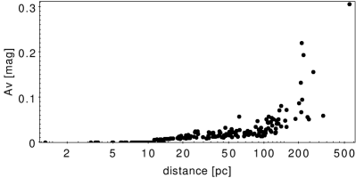
Figure 3: Extinction $A_{\rm V}$ deduced from 3D maps of Vergely et al. (2022) as a function of distance, for the 201 targets.

3.4 SED fitting and bolometric fluxes

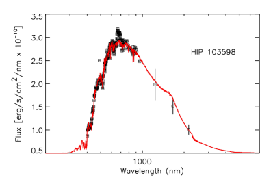
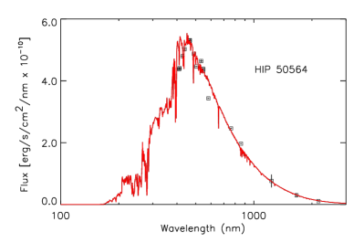
Figure 4: Example of fits of the observed (reddened) data to the (reddened) semi-empirical spectra for HIP 103598 (left) and HIP 50564 (right). The bolometric flux is calculated by integrating the un-reddened spectrum. The bottom panels illustrate the distribution of $\chi^{2}_{R}$ versus $F_{\rm bol}$ for the 400 simulations for the two stars with the 16^th, 50^th (median), and 84^th percentiles indicated by the dashed lines.

Although the observed fluxes compiled for the GBS cover a wide range of wavelength, some extrapolation of the SED is needed to integrate the full distribution and measure the total flux from the star received at the Earth, $F_{\rm bol}$. To do so we followed the SED fitting method previously used by Creevey et al. (2015) and Ligi et al. (2016), based on the BASEL empirical library of spectra (Lejeune et al., 1997), a highly cited library in the astrophysical community. Our choice for these models is based upon the work in Creevey et al. (2015) where one star was analysed in detail using different approaches and models. A 1% flux difference was found using the BASEL and PHOENIX libraries, with the former being in best agreement with other literature results using different methodologies.

The BASEL library covers the following parameter ranges: $3\,500<T_{\rm eff}<50\,000$ K, $0.00<\log g<5.00$, and –5.0 $<$ [M/H] $<$ +1.0. It extends to 2 000 K for a subset of the $\log g$ and [M/H]. The wavelength range spans 9.1 to 160 000 nm on a non-evenly sampled grid of 1221 points, with a mean resolution of 100 nm in the UV and 200 nm in the visible. Beyond 10 000 nm the resolution is 20 000 nm and to avoid issues with numerical integration we interpolate on a log scale before performing the integration. A Levenberg-Marquardt minimisation algorithm finds the optimal template that fits the observed flux points. $F_{\rm bol}$ is then calculated by integrating the optimal fitted spectrum. Recent improvements of the method include the weighting of the fluxes and the determination of $F_{\rm bol}$ uncertainties through Monte-Carlo simulations.

The parameters of the model are the atmospheric parameters: $T_{\rm eff}$, $\log g$, [Fe/H], the extinction, and the scaling factor (stellar radius scaled according to the distance). We used the atmospheric parameters from PASTEL to initialise the minimization and the extinction from Sect. 3.3. To account for extinction in our method we implemented the IDL routine ccm_unred which dereddens theoretical fluxes, and requires colour-excess on input. To convert extinction to colour-excess we adopted $R_{0}=3.1$. Most of these stars are nearby and as such have little or no extinction. In order to be complete in our analysis, in the catalogue available at the CDS we also provide $F_{\rm bol}$ for the full sample of stars by assuming zero extinction.

All of the above parameters can be fitted, but in practice due to degeneracies between the parameters, the $T_{\rm eff}$ and the scaling factor are the only free parameters, while $\log g$, [Fe/H], and the extinction are fixed each time a minimization is performed. In order to include the impact of the uncertainties of the parameters $\log g$ and [Fe/H], and of the fluxes, we performed a bootstrapped-based method where we (a) perturbed these parameters by their uncertainty multiplied by a random number drawn from a Gaussian distribution, and (b) perturbed the fluxes by their uncertainties using the same approach. These simulations were done 400 times where 400 was a balance between computing time and having a significant sample size (the results with 200 simulations were equivalent within the uncertainties and the standard deviation of the 400 simulations reproduced the uncertainties of the atmospheric parameters). For the fitted parameters, the result is a distribution of stellar parameters that fit the observational data, and from these fitted parameters we integrated the corresponding semi-empirical flux distribution. We therefore obtained a distribution of $F_{\rm bol}$ for each star, and from these distributions we calculated the medians and the symmetric 68% confidence intervals, and report half of the latter as the uncertainty.

Two examples of the data and the best-fitted model SED are shown in Fig. 4, left and right panels. The left is an example of a star with many observational points (in this case HIP103598), while the right panel shows an example where relatively few data points are available; in this case HIP50564. The lower panels show the distribution of the fitted $F_{\rm bol}$ and the individual $\chi^{2}$ values from the 400 Monte Carlo simulations, along with the value of the adopted median and 16 and 84 percentile confidence levels (dashed lines). We defined the uncertainty as the half of the distance between the upper and lower confidence levels.

The distribution of $F_{\rm bol}$ and relative uncertainties is shown in Fig. 5. The histogram of uncertainties shows a clear peak in the first bin corresponding to uncertainties lower than 0.5%. The relative uncertainties have a median value of 1.4%, and they are lower than 10% except for two stars, namely HIP8837 ($\psi$ Phe) and HIP14135 ($\alpha$ Cet). These two M giants combine a low $T_{\rm eff}$ and a lack of spectrophotometric data which make their SED poorly constrained, resulting in a relative uncertainty of about 21% and 18% respectively. They had uncertain $F_{\rm bol}$ in Paper I as well. We note that the stars with uncertainties larger than 4% have their SED made of broad-band photometry only, while the majority of stars have spectrophotometry from Gaia and/or Pulkovo, resulting in a very precise $F_{\rm bol}$ determination.

In this procedure to determine $F_{\rm bol}$, we use $\log g$ and metallicity from the PASTEL catalog, a compilation of literature work. We have evaluated the impact of not knowing precisely these parameters. To do so, we made two tests. One test is to adopt a large uncertainty of 0.15 on both $\log g$ and [Fe/H]  inducing a different distribution of the fitted $F_{\rm bol}$ from the 400 Monte Carlo simulations. The other test is to change the literature values of $\log g$ and [Fe/H] by an amount of 0.15 dex, in the eight possible configurations, for seven stars selected to cover the parameter space. In this test, the largest effect ($<$1%) is reached when adding 0.15 dex to [Fe/H] for the hottest stars. Varying $\log g$ has more effect on the coolest stars. When combining the variations of $\log g$ and [Fe/H] the effect remains at the level of 1% for the coolest and the hottest stars. Interestingly the most metal-poor star chosen for that test, HIP48152, is less affected by a change of $\log g$ and [Fe/H]. In the other test, enlarging the $\log g$ and [Fe/H] uncertainties in the Monte-Carlo simulations also has a low impact on the derived value of $F_{\rm bol}$. We note four stars with $F_{\rm bol}$ changed by 1-2%, while 90% of the sample changes by less than 0.5%. We conclude that our procedure weakly depends on the input values of $\log g$ and [Fe/H]. A change of 1% in $F_{\rm bol}$ induces a change of 0.2% on $T_{\rm eff}$. However a more rigorous treatment will be performed through iterations once the spectroscopic analysis of the targets will be performed to derive [Fe/H] homogeneously (Paper VIII in preparation). This will lead to self-consistent parameters.

In Paper I, the $F_{\rm bol}$ values of the V1 stars were compiled from the literature and therefore not as homogeneous as here. This is another important improvement of the GBS V3, in addition to the larger number of stars. We still have a good agreement between V1 and V3, with a slight offset of 1.4%, and a typical dispersion of 2.1% (median absolute deviation, MAD).

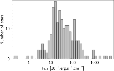
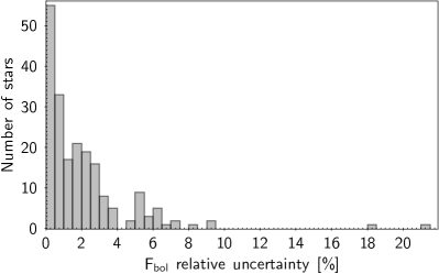
Figure 5: Histogram of $F_{\rm bol}$ (top panel) and its relative uncertainties (bottom panel).

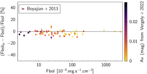
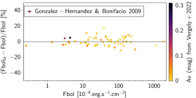
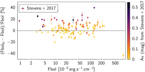
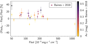
Figure 6: Comparison of $F_{\rm bol}$ obtained in this work with literature. The colour code relates to the extinction. Several extreme outliers are out of the figure boundaries but they are discussed in the text.

Our approach is similar to that of Boyajian et al. (2013) and Baines et al. (2018) who collected broadband photometric measurements available in the literature, extended by spectrophotometry when available. They also applied the SED fitting method with reference templates taken from the library of Pickles (1998) which is made of observed spectra, whereas we used a hybrid library of synthetic stellar spectra calibrated from observations (Lejeune et al., 1997). Another difference comes from the Gaia spectrophotometry recently made available, which constrains very well the SED shape in the optical range. We have 66 stars in common with Boyajian et al. (2013) and 24 with Baines et al. (2018). The $F_{\rm bol}$ comparison is shown in Fig. 6. The agreement with Boyajian et al. (2013) is very good, with differences within 10%. On average our $F_{\rm bol}$ values are higher than their values by 3.3%, with a typical dispersion of 2.5% (MAD). The offset does not seem correlated with extinction which is lower than 0.03 mag for the stars in common according to our estimations, and that they have not considered given the close distance of the stars. It is likely that the small offset observed between our $F_{\rm bol}$ determinations and those of Boyajian et al. (2013) is related to their use of magnitudes from photometric catalogues, with a maximum of 17 values per star and less than 12 values in most cases, while we have typically ten times more flux values, mostly from Gaia spectrophotometry, providing SEDs of better quality. In addition they did not take photometric uncertainties into account for the fit, while we do. Baines et al. (2018) determine a high extinction for some stars which seems correlated with a larger positive offset. HIP47431 and HIP90344 are the most extreme cases with $A_{\rm V}$=0.7 mag and $A_{\rm V}$=0.54 mag respectively in Baines et al. (2018) while we get $A_{\rm V}$=0.02 mag and $A_{\rm V}$=0.03 mag from the 3D maps of Vergely et al. (2022), leading to a difference of 50% and 37% on $F_{\rm bol}$ (HIP47431 is not shown in Fig. 6). Considering the 24 stars in common, Baines et al. (2018) find $F_{\rm bol}$ higher than us by 7.6% (median) with a dispersion of 6.6% (MAD).

We also compared our $F_{\rm bol}$ determinations to those of González Hernández & Bonifacio (2009) who implemented the infrared flux method (IRFM) based on 2MASS magnitudes (see Fig. 6). The 61 stars in common generally agree well with an offset less than 1% and a dispersion of 3.9% (MAD). The extinction is low for the majority of these nearby stars.

Finally, we also made a comparison with the catalog of empirical bolometric fluxes and angular diameters of 1.6 million Tycho-2 stars built by Stevens et al. (2017) which has 119 stars in common with us. This work is based on the flux-colour relations of Casagrande et al. (2010) with $T_{\rm eff}$ and $A_{\rm V}$ being determined separately in an iterative way. Their $F_{\rm bol}$ are globally larger than ours by 4.9%, with a dispersion of 7.5% (MAD). Similarly to the tendency observed in the comparison with Baines et al. (2018), the larger differences correspond to stars with the largest values of $A_{\rm V}$ in Stevens et al. (2017) which significantly differ from our lower extinctions. Eight stars do not appear in Fig. 6, given their difference larger than 50%, up to 360% for HIP112731 and HIP96837. They are found highly reddened by Stevens et al. (2017) with $A_{\rm V}$$\geq$0.6 mag, up to more than 2 mag for the two most extreme stars HIP112731 and HIP96837. We therefore suspect that some extinctions are overestimated by Stevens et al. (2017) and Baines et al. (2018), leading to overestimated bolometric fluxes.

3.5 Assessment of $T_{\rm eff}$

We computed the fundamental $T_{\rm eff}$ of each star by applying Eq. (1) with the values of $\theta_{\rm LD}$ and $F_{\rm bol}$ obtained as described above. $T_{\rm eff}$ uncertainties were deduced by propagating the $\theta_{\rm LD}$ and $F_{\rm bol}$ uncertainties in Eq. (1). We consider here the 192 stars with a direct value of $\theta_{\rm LD}$. The resulting uncertainties on $T_{\rm eff}$ span 5 K to 183 K, with a median value of 43 K (see histogram in Fig. 7). Only four giants present a relative uncertainty larger than 3% (absolute uncertainty larger than 150 K): the two M giants HIP8837 ($\psi$ Phe) and HIP14135 ($\alpha$ Cet) previously mentioned for their large $F_{\rm bol}$ uncertainty resulting in $T_{\rm eff}$ uncertainties of $\sim$5%, and the K giants HIP25993 and HIP14838 previously mentioned for their large uncertainty on $\theta_{\rm LD}$ resulting in $T_{\rm eff}$ uncertainties of $\sim$3.5%. These four stars clearly stand as outliers in

Fig. 8 which shows how the relative uncertainties on $\theta_{\rm LD}$ and $F_{\rm bol}$ propagate on $T_{\rm eff}$. In order to reach a 1% accuracy on $T_{\rm eff}$ one should restrict the sample to stars with measurements better than $\sim$2% in $\theta_{\rm LD}$ and $\sim$4% in $F_{\rm bol}$. We have 127 stars fulfilling this condition, while 179 of the 192 stars have $T_{\rm eff}$ uncertainties better than 2%.

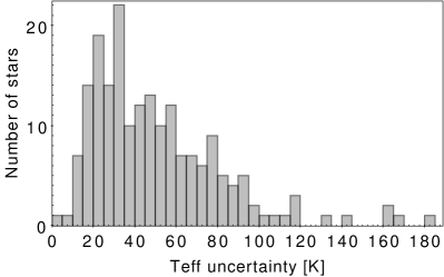
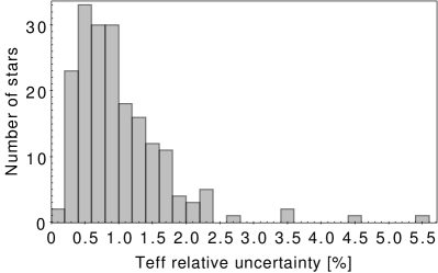
Figure 7: Histogram of $T_{\rm eff}$ absolute (top panel) and relative (bottom panel) uncertainty. The four outliers with $T_{\rm eff}$ uncertainty larger than 150 K (or 3%) are discussed in the text.

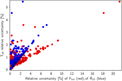
Figure 8: Propagation of $\theta_{\rm LD}$ and $F_{\rm bol}$ relative uncertainties on $T_{\rm eff}$.

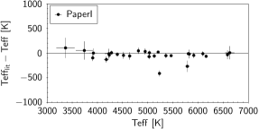
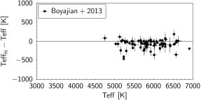
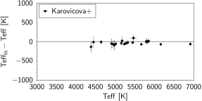
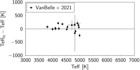
Figure 9: Comparison of our fundamental determinations of $T_{\rm eff}$ with other fundamental determinations from the literature in Paper I and Boyajian et al. (2013); Karovicova et al. (2020, 2022a, 2022b); van Belle et al. (2021).

Table 2: Median difference (MED) and median absolute deviation (MAD) between direct determinations of $T_{\rm eff}$ from the literature and our values (literature minus this work), for N stars in common.

Reference	N	MED	MAD
		(K)	(K)
Heiter et al. (2015) - Paper I	28	-26	32
Boyajian et al. (2013)	82	-59	58
Karovicova et al. (2020, 2022a, 2022b)	21	-39	30
van Belle et al. (2021)	17	61	77

In Fig. 9 we compare our values of $T_{\rm eff}$ to other direct determinations from the literature, including those in Paper I. The values of offset (median difference) and dispersion (MAD) are given in Table 2. The dispersion is remarkably low (MAD$\simeq$30 K) for the comparison to Paper I and Karovicova et al. (2020, 2022a, 2022b), our determinations being larger by 26 K and 39 K respectively. The agreement is therefore at the 1% level in general. The two outliers in the comparison to Paper I (upper left panel of Fig. 9) are the metal-poor benchmark stars HIP57939 and HIP76976 (HD103095 and HD140283). Our new $T_{\rm eff}$ values are about 400 K and 250 K higher than in Paper I, where their sub-mas angular diameters were quoted as very uncertain. Both stars have been remeasured by Karovicova et al. (2018, 2020) leading to more precise $\theta_{\rm LD}$ and higher $T_{\rm eff}$. Our determination for HD103095 ($T_{\rm eff}$=5235$\pm$18 K) is larger by 61 K than that of Karovicova et al. (2020). Since we use their determination of $\theta_{\rm LD}$, the difference is only due to $F_{\rm bol}$. As noted in Sect. 3.1, the angular diameter of HD103095 measured by Karovicova et al. (2020) from the combination of two instruments is very reliable. For HD140283 we find $T_{\rm eff}$=5788$\pm$45 K, lower by 4 K than their value. Three other stars differ by 2-3% from Paper I: $\psi$ Phe, 61 Cyg B and $\gamma$ Sge. Only $\gamma$ Sge has a new angular diameter measured by Baines et al. (2021), while for the other ones we used the same $\theta_{\rm LD}$ as in Paper I, indicating that the difference comes from the new determination of $F_{\rm bol}$, which we expect to be more accurate than the previous determination.

Table 2 and Fig. 9 exhibit larger discrepancies in the comparison to Boyajian et al. (2013) with an offset of 59 K and a scatter of 58 K. We note that we have 66 stars in common but 82 measurements since Boyajian et al. (2013) provide a compilation of their own $\theta_{\rm LD}$ together with other values from the literature (we removed discrepant values quoted by them for HD146233 and HD185395). Among the stars that differ by more than 300 K, we have again HD103095 which is the largest outlier. As explained above, the recent $\theta_{\rm LD}$ determination by Karovicova et al. (2020) gives a higher $T_{\rm eff}$ which is in better agreement with our value for that star. For HIP61317 Boyajian et al. (2013) give two values of $T_{\rm eff}$, only one being in significant disagreement with ours. For HIP89348 our values of $F_{\rm bol}$ and $\theta_{\rm LD}$ (the latter adopted from Ligi et al. 2016) are larger and smaller, respectively, by $\sim$10% than those of Boyajian et al. (2013), resulting in a significantly different $T_{\rm eff}$. Our value of $T_{\rm eff}$=6569$\pm$69 K seems however more consistent with spectroscopic values listed in the PASTEL catalogue than their lower value of $T_{\rm eff}$=6221$\pm$39 K.

The comparison to van Belle et al. (2021) gives an offset of 61 K, this time our values being lower, with a dispersion of 77 K. This relies on 17 giants in common. These large differences could partly be due to disagreement in extinction values for some stars. We note four stars (HIP7607, HIP111944, HIP74666, HIP3031) that van Belle et al. (2021) found significantly reddened ($A_{\rm V}$ from about 0.15 to 0.30 mag) while our $A_{\rm V}$ determinations are below 0.05 mag. This possibly explains the $T_{\rm eff}$ differences from 150 K to 220 K. On the other hand, HIP22453 has $A_{\rm V}$=0.36 mag in van Belle et al. (2021) and $A_{\rm V}$=0.08 mag in our work, but the $T_{\rm eff}$ difference is only 31 K.

We note that we use the same determination of angular diameter as in the literature for some of the stars. Hence, the comparison data sets are not completely independent from ours.

4 Surface gravity

We determined the surface gravity $\log g$ with the fundamental relation expressed as:

$$\centering\log g=\log\left(\left(\frac{M}{M_{\odot}}\right)\left(\frac{R}{R_{\odot}}\right)^{-2}\right)+\log g_{\odot}\@add@centering$$ (2)

where $M/M_{\odot}$ and $R/R_{\odot}$ are the mass and radius of the star in solar units. For the Sun, we adopt for the surface gravity $\log g_{\odot}=4.4380\pm 0.0002$ dex determined in Paper I. The linear radius of each star is deduced from its angular diameter (see Sect. 3.1) and its distance is inferred from its parallax (see below). Masses, which cannot be directly measured, are estimated from evolutionary tracks, using our fundamental $T_{\rm eff}$, luminosities (from $F_{\rm bol}$ and parallaxes), radii (from $\theta_{\rm LD}$ and parallaxes) and metallicities from the literature as input. We consider in this section the full sample of 201 GBS V3, including the nine stars with an indirect $\theta_{\rm LD}$.

4.1 Parallaxes, linear radii and luminosities

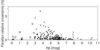
Figure 10: Distribution of parallax relative uncertainties versus Hipparcos magnitudes for the GBS V3 sample. Parallaxes are mainly from Gaia DR3, but from Hipparcos for 8 stars (open squares), and from Akeson et al. (2021) for $\alpha$ Cen A & B (filled squares).

The parallax of the stars is needed to convert their angular diameter into linear radius, and their bolometric flux into luminosity. All the targets have a Hipparcos parallax, and the majority of them have also an even more precise and accurate Gaia DR3 parallax. Only four stars have a Gaia parallax with an uncertainty larger than 3%, the largest value being 6% for HIP55219. The ten brightest stars not in Gaia DR3 have a precision of their Hipparcos parallax better than 3.5%. For $\alpha$ Cen A & B (HIP71683 & HIP71681) we adopt the high precision determination by Akeson et al. (2021) instead of the Hipparcos one. Figure 10 shows the distribution of the parallax relative uncertainties as a function of the Hipparcos magnitude Hp. The four faintest stars with Hp$>$8 mag have an indirect $\theta_{\rm LD}$. We applied the zero-point correction derived by Lindegren et al. (2021) to the Gaia parallaxes.

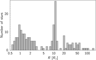
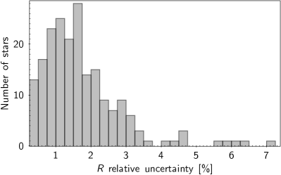
Figure 11: Histogram of linear radii $\mathit{R}$ (top panel) and their relative uncertainty (bottom panel).

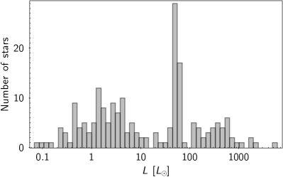
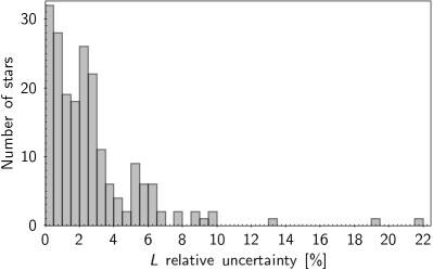
Figure 12: Histogram of luminosities $\mathit{L}$ (top panel) and their relative uncertainty (bottom panel).

With parallaxes $\pi$ and $\theta_{\rm LD}$ we computed linear radii $\mathit{R}$ and their uncertainties, while we used parallaxes and $F_{\rm bol}$ to compute luminosities $\mathit{L}$ and their uncertainties. Adopting the solar radius and luminosity from the 2015 B3 IAU resolution the equations are:

$$\centering\frac{\mathit{R}}{\mathit{R}_{\odot}}=\frac{1}{0.00930093}\times\frac{\theta_{\rm LD}}{\pi}\@add@centering$$ (3)

$$\centering\frac{\mathit{L}}{\mathit{L}_{\odot}}=312.564\times\frac{F_{\rm bol}}{\pi^{2}}\@add@centering$$ (4)

with $\theta_{\rm LD}$ and $\pi$ expressed in mas, and $F_{\rm bol}$ in $10^{-8}$ erg s^-1 cm^-2.

The radii of the GBS V3 span 0.6 to $\sim$140 $R_{\odot}$ (see Fig. 11). The luminosities span 0.08 to nearly 6000 $L_{\odot}$ (see Fig. 12).

Solar-like oscillations provide robust constraints to the radius of G and K dwarfs and giants (Chaplin & Miglio, 2013), giving us an opportunity to compare our determinations with others obtained in a different way. We estimated seismic radii using the following scaling relation (e.g. Miglio, 2012) when the asteroseismic parameters, the so-called large frequency separation $\Delta\nu$ and the frequency of maximum oscillation power $\nu_{\rm max}$, were available:

$$\frac{R}{R_{\odot}}\approx\left(\frac{\nu_{\rm max}}{\nu_{{\rm max}\odot}}\right)\left(\frac{\Delta\nu}{\Delta\nu_{\odot}}\right)^{-2}\left(\frac{T_{\rm eff}}{T_{{\rm eff},\odot}}\right)^{1/2},$$ (5)

where we adopt the fundamental $T_{\rm eff}$ determined in Sect. 3 and the solar parameters as in Paper I: $\Delta\nu_{\odot}=135.229\pm 0.003\leavevmode\nobreak\ \mu$Hz, $\nu_{\rm max,\odot}=3160\pm 40\leavevmode\nobreak\ \mu$Hz, $T_{\rm eff,\odot}=5771\pm 1$K. We have compiled $\Delta\nu$ and $\nu_{\rm max}$ from the literature and found determinations of both parameters for 37 stars. The comparison is shown in Fig. 13. There is a small systematic offset, the fundamental radii being larger than the seismic ones by 0.7%, with a typical dispersion (MAD) of 3.3%. Several stars show discrepancies larger than 10%, up to 22% for HIP92984. There is however an ambiguity about the seismic parameters of HIP92984, measured by Mosser et al. (2009) from CoRoT observations, because Huber et al. (2012) did not detect solar-like oscillations. The other discrepant stars have error bars that still give an agreement at the 3$\sigma$ level. We also note that Sharma et al. (2016) and Hon et al. (2022) proposed some corrections to the scaling relations to obtain a better agreement for giants. It is however out of the scope of this paper to apply such corrections. We retain from this comparison the general good agreement, with no systematics, between our values and seismic ones, at the level of $\sim$4%.

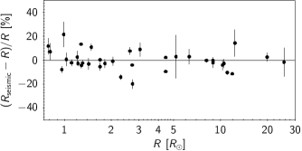
Figure 13: Linear radius difference between our determination of $\mathit{R}$ from Eq. (3), and seismic estimations from Eq. (5).

Figure 14 shows our derived luminosities compared to those available for 36 stars in the Gaia DR3 Golden Sample of Astrophysical parameters for FGKM stars (Gaia Collaboration et al., 2023a). Gaia luminosities were computed from the parallax, the G magnitude and a bolometric correction (Creevey et al., 2023) and are therefore different from our determinations, although not completely independent. The three most luminous stars in common are found brighter by Gaia by more than 10%, up to 30% for HIP70791, known as a horizontal branch star. Only that star shows a discrepancy significantly larger than 3$\sigma$. We note six other stars with Gaia luminosities significantly larger than our values, with differences ranging from 5% to 10%. These discrepancies cannot be explained by the extinction that we find negligible for these nine stars. For the other stars, we find luminosities slightly larger than those from Gaia, by 0.35% (median), with a typical dispersion of 0.9% (MAD).

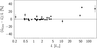
Figure 14: Luminosity difference between our determinations $\mathit{L}$ from $F_{\rm bol}$ and distance, and Gaia DR3 estimations based on G magnitudes and bolometric corrections for 36 stars in common in the Golden Sample of Astrophysical Parameters (Gaia Collaboration et al., 2023a).

4.2 Masses

Masses were computed with the SPInS code (Lebreton & Reese, 2020) implemented with the stellar evolutionary tracks from BaSTI (Pietrinferni et al., 2004, 2006), and from STAREVOL (Lagarde et al., 2012, 2017). We implemented the two grids in order to make comparisons owing to the different behaviour of the tracks in some parts of the HR-diagram (HRD), like the clump. The determinantion of the logg is less accurate at clump luminosity (logg$\simeq$2.2) because this is a point in the HR diagram where the evolutionary tracks of different masses and [Fe/H] overlap. In the following, we detail the main differences between these two grids that may have an impact on the position on the HRD and thus on the mass determination with SPInS.

• BaSTI - We use stellar tracks coming from the non-canonical grid covering a mass range between 0.5 M_⊙ and 10.0 M_⊙ and a metallicity range [Fe/H] $\in$ [$-2.27$, +0.40] without $\alpha$-enhancement. This grid takes into account core convective overshooting during the H-burning phase. The overshoot parameter is set to 0.2 for a stellar mass higher than 1.7 M_⊙, no overshooting is considered for a mass lower than 1.1 M_⊙, and a linear variation is assumed in-between. The solar mixture comes from Grevesse et al. (1993). We tried the $\alpha$-enhanced tracks ([$\alpha$/Fe]=+0.4) for metal-poor stars ([Fe/H]¡-0.70 dex) leading to masses higher by 30% on average. However, as explained later, we got a wrong mass for $\mu$ Cas, the only metal-poor binary with a reliable dynamical mass. This convinced us to adopt the tracks without $\alpha$-enhancement for the whole sample.

• STAREVOL - This stellar grid covers a mass range between 0.6 and 6.0 M_⊙ and a metallicity range [Fe/H] $\in$ [$-2.14$, +0.51] without $\alpha$-enhancement, with the exception of [Fe/H]=-2.14 and -1.2 where [$\alpha$/Fe]=+0.3. Except for convection, additional mixing effects such as rotation-induced mixing are not taken into account. The overshoot parameter is set to 0.05 or 0.10 for stars with masses below or above 2.0 M_⊙, respectively; no overshooting is considered for masses lower than 1.1 M_⊙. The stellar grid is constructed using the solar mixture coming from Asplund et al. (2009).

The Kroupa initial mass function (Kroupa, 2001; Kroupa et al., 2013, IMF) was used as a prior, as well as a truncated uniform star formation rate between 0 and 13.8 Gyr, that is, roughly the age of the Universe. The stellar properties used as an input to SPInS are: (1) our fundamental $T_{\rm eff}$ determinations (Sect. 3); (2) luminosities deduced from $F_{\rm bol}$ and parallaxes; (3) metallicities from the literature, and (4) radii deduced from $\theta_{\rm LD}$ and parallaxes. Radii are not independent of $T_{\rm eff}$ and luminosities, but still add a useful constraint to the mass since the correlations are lost in the way we determined the three parameters. The resulting masses and their uncertainties are shown in Fig. 15. Most of the stars have masses $<2$ ${\rm M}_{\odot}$ but STAREVOL finds more stars in the range 2–2.5 ${\rm M}_{\odot}$ than BaSTI. STAREVOL gives a more extended distribution of relative uncertainties with fewer very low values, and five stars within 30-55%.

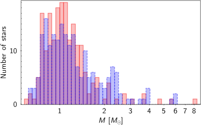
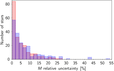
Figure 15: Histogram of masses (top panel) and their relative uncertainty (bottom panel), red for BaSTI, blue for STAREVOL.

For the validation of the mass determination, we compared the SPInS results to other determinations. This includes dynamical masses of binary stars, seismic masses, as well as mass determinations based on evolutionary tracks and methods different from those we used.

Dynamical masses are available for four stars, $\mu$ Cas, $\alpha$ Cen A & B, and Procyon. We did not consider 61 Cyg A & B since their masses are not well established (Kervella et al., 2022). The comparison to SPInS masses is shown in Fig. 16. The orbit of the binary $\alpha$ Cen has been studied by Akeson et al. (2021) who determined masses of 1.0788$\pm$0.0029 $M_{\odot}$ and 0.9092$\pm$0.0025 $M_{\odot}$ for the A (HIP71683) and B (HIP71681) components, respectively. The agreement is at the 0.4% level for the STAREVOL mass and 3.4% for the BaSTI mass, for the component A. Both sets of evolutionary tracks give masses that differ by 5% for the B component, in opposite directions. The dynamical mass of the metal-poor ([Fe/H]=-0.83 dex) visual binary $\mu$ Cas (HIP5336) results from an astrometric study with the Hubble Space Telescope by Bond et al. (2020) who determined a value of 0.7440$\pm$0.0122 $M_{\odot}$. BaSTI and STAREVOL underestimate it by 4% and 1.3% respectively. Running SPInS with the $\alpha$-enhanced BaSTI tracks ([$\alpha$/Fe]=+0.4) for that star led to an overestimation of its mass by 32%. This convinced us not to adopt the $\alpha$-enhanced tracks for metal-poor stars. Hence, we have opted to exclusively rely on the BaSTI tracks that do not incorporate any alpha-enrichment. This underscores the importance of presenting mass values obtained from both BaSTI and STAREVOL tracks, since it offers an understanding of the inherent errors linked to relying solely on a single stellar evolution model. The orbit of Procyon (HIP37279) based on Hubble Space Telescope astrometry (Bond et al., 2015, 2018), yields a dynamical mass of 1.478$\pm$0.012 $M_{\odot}$. The BaSTI mass differs by 0.9% while the STAREVOL mass is lower by 2.6%. There is therefore a satisfactory agreement between the SPInS masses and the dynamical masses for these four stars, whatever the set of evolutionary tracks, considering the few constraints we use with the models, and given the inherent model assumptions of e.g. the chemical enrichment law which constrain the position of the tracks in the HRD.

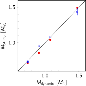
Figure 16: Comparison of masses determined with SPInS (red dots for BaSTI, blue open squares for STAREVOL) to dynamical masses for $\mu$ Cas, $\alpha$ Cen B, $\alpha$ Cen A and Procyon, ordered by increasing mass.

We estimated seismic masses using the following scaling relation (e.g. Miglio, 2012) for the 37 stars having a determination of the asteroseismic parameter $\Delta\nu$ available in the literature (see Sect. 4.1 for the solar values)

$$\frac{M}{M_{\odot}}\approx\left(\frac{\Delta\nu}{\Delta\nu_{\odot}}\right)^{2}\left(\frac{R}{R_{\odot}}\right)^{3},$$ (6)

where R is the linear radius computed in Sect. 4.1. The resulting comparison is shown in Fig. 17. Although the agreement between SPInS and seismic masses is good in general in the range 1–1.5 M_⊙, there is a trend in the sense that SPInS tends to overestimate masses smaller than 1 M_⊙ and to underestimate those larger than 1.5 M_⊙. This is true for both sets of evolutionary tracks, with more outliers with STAREVOL. However, seismic masses may not necessarily be more accurate than those deduced from evolutionary tracks, given that the range of validity of the scaling relation is not yet clear (e.g. Sharma et al., 2016).

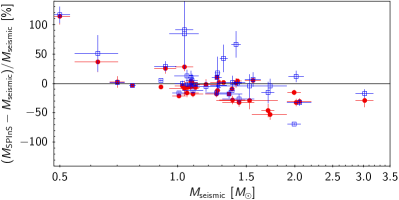
Figure 17: Comparison between masses from SPInS (red dots for BaSTI, blue open squares for STAREVOL) and seismic masses from Eq. (6).

We also compared the two sets of SPInS masses to masses from the literature, based on different evolutionary tracks and methods. Figure 18 shows comparisons to masses from Paper I, Baines et al. (2018) and Boyajian et al. (2013). In Paper I masses were determined by visual interpolation in two grids, the Padova grid (Bertelli et al., 2008, 2009) and the Yonsei-Yale grid (Yi et al., 2003; Demarque et al., 2004), the adopted value being the average of the two. Baines et al. (2018) used a Bayesian method with the PARSEC isochrones developed by da Silva et al. (2006); Bressan et al. (2012). Boyajian et al. (2013) used the Yonsei-Yale isochrones. The resulting comparisons reflect the nature of the stars in common, with a good agreement for dwarfs and a large dispersion for giants. A larger dispersion is expected for giants, in particular at the clump, because of the overlap of the evolutionary tracks of different masses and [Fe/H]. Degeneracies in evolutionary tracks of evolved stars can also lead to different masses for a giant depending on whether it is on the red-giant branch or on the horizontal branch. The sample of Boyajian et al. (2013) is made of dwarfs and exhibits a small dispersion, despite a few outliers with STAREVOL. The sample of Baines et al. (2018) is mostly made of giants and exhibits a large dispersion, while GBS V1 are a mixture of dwarfs and giants.

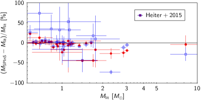
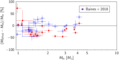
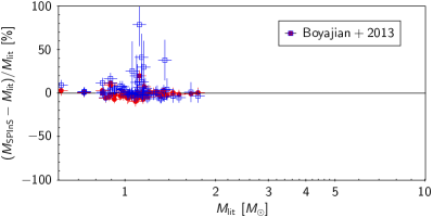
Figure 18: Comparison of masses determined with SPInS (red dots for BaSTI, blue open squares for STAREVOL) to those available in the literature, also based on evolutionary tracks.

Figure 19 shows our derived masses compared to those available for 30 stars in the Gaia DR3 Golden Sample of Astrophysical parameters for FGKM stars (Gaia Collaboration et al., 2023a). Gaia masses were derived by comparing Gaia photometric effective temperatures and Gaia luminosities to BaSTI solar metallicity stellar evolution models (Hidalgo et al., 2018; Creevey et al., 2023), and are therefore similar to our determinations. We find an excellent agreement between our two sets of masses and the Gaia ones, except for the three stars in common with the highest masses ($\gtrsim$1.5 M_⊙), and one outlier within the STAREVOL set.

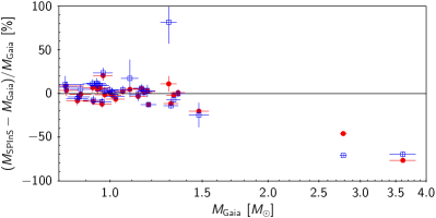
Figure 19: Comparison between masses from SPInS (red dots for BaSTI, blue open squares for STAREVOL) and masses from the Gaia Golden Sample of Astrophysical Parameters (Gaia Collaboration et al., 2023a).

From the above comparisons, there is no strong evidence that one set of evolutionary tracks is better than the other one. Therefore we provide the two masses and their uncertainties in the catalogue available at the CDS.

In this procedure to determine masses we need metallicities as input for SPInS. We have used [Fe/H] values from the literature which are not homogeneous and therefore we have evaluated their impact on the resulting masses. We made two tests similar to those made for $F_{\rm bol}$. One test is to adopt a large uncertainty of 0.15 on [Fe/H] for all the stars, much larger than the original ones. The other test is to add or subtract 0.15 dex to the literature values of [Fe/H] for seven stars selected to cover the parameter space. Enlarging the metallicity uncertainty to 0.15 dex affects mainly the clump giants. Based on the BASTI tracks, only 5 stars in our sample have their mass affected by more than 30%, and only 8 stars if we consider the STAREVOL tracks. The most critical stars are not common from one set to the other. This reinforces the interest of considering the masses computed by the two sets of stellar evolution models. Such differences could be explained by different inputs in the computation of the evolutionary tracks (e.g. mass loss, atmosphere models, etc.) which change the position in the HRD. It should be noted that at least 90% of the stars in our sample experience a mass variation less than 10%, while three quarters of the sample remain below 5%, whatever the set of stellar models taken into account. Changing the value of [Fe/H] by $\pm$0.15 dex for seven stars leads to a similar conclusion: the dwarfs are not affected, whatever their metallicity, while changes occur among giants. However, due to the dependency of $\log g$ on the logarithm of mass in Eq. (2), in the worst cases where the mass is changed by 30%, the impact on $\log g$ is limited to 0.11 dex and up to 0.5 dex for the most critical cases.

4.3 Assessment of $\log g$

We computed the fundamental $\log g$ of each star by applying Eq. (2) with the values of mass from SPInS, with both evolutionary tracks BaSTI and STAREVOL, and the radius deduced from $\theta_{\rm LD}$, with the propagation of their uncertainties. We consider here the 201 stars of the sample. The resulting uncertainties on $\log g$ span from 0.004 to 0.13 (BaSTI) and 0.23 dex (STAREVOL), with a median value of 0.02 dex. Figure 20 shows the comparison of $\log g$ determinations, using the mass from SPInS with BaSTI or STAREVOL. The agreement is excellent for dwarfs with $\log g$$>$4. Below that value, $\log g$ from STAREVOL is systematically larger by 0.06 dex than $\log g$ from BaSTI, with an exception around $\log g$_STAREVOL=2.3.

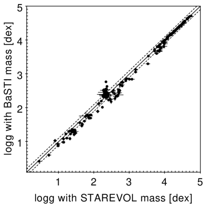
Figure 20: Comparison of $\log g$ determinations, using masses from SPInS with BaSTI or STAREVOL. The area between the two dashed lines indicates an agreement within 0.1 dex.

Following the comparisons made in the previous sections, for radii and masses, we used the seismic data to determine $\log g$ in another and independent way, through the relation that gives $\log g$ as a function of the maximum of the power spectrum of oscillation frequencies, $\nu_{\rm max}$, available for 42 stars, and the effective temperature:

$$\log g\approx\log\nu_{\rm max}+0.5\log T_{\rm eff}-\log\nu_{\rm max,\odot},-0.5\log T_{\rm eff,\odot}+\log g_{\odot},$$ (7)

The comparison of seismic and fundamental $\log g$ is shown in Fig. 21. For dwarfs, typically $\log g$${}_{\rm seismic}>$3.8 dex, the agreement is very good except for one star, HIP92984. For this star we find $\log g$=4.48 dex with BaSTI and STAREVOL masses, while the seismic $\log g$ is significantly lower, $\log g$=4.23. We have pointed out the ambiguity about the seismic parameters of that star in the previous section. If this star is excluded, the differences between seismic and fundamental $\log g$ of dwarfs have a MAD of 0.02 dex. For giant stars, the dispersion is larger (MAD=0.07 dex), with $\log g$ based on BaSTI lying slightly below the seismic values (median offset of $-0.06$ dex), while the $\log g$ based on STAREVOL tend to lie above (median offset of 0.01 dex). A few outliers, reaching nearly 0.5 dex, correspond to stars with one of the two masses giving a disagreement with the seismic $\log g$ but not the other one. From that comparison, we cannot say that the agreement is better with BaSTI or with STAREVOL masses.

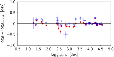
Figure 21: Comparison of our fundamental values of $\log g$ to those determined from $\nu_{\rm max}$ and our fundamental $T_{\rm eff}$. Red dots for SPInS masses using BaSTI models, blue open squares for STAREVOL models.

We also compare our $\log g$ determinations with those in Paper I and in Karovicova et al. (2020, 2022a, 2022b) in Fig. 22. Offsets are negligible while dispersions (MAD) are 0.04 dex for Paper I, whatever the tracks. The values of $\log g$ generally agree well within the error bars except for one star, HIP37826 (Pollux), where the STAREVOL mass gives a discrepant $\log g$. The dispersions are 0.02 and 0.04 dex, using masses from BaSTI and STAREVOL respectively, for Karovicova et al.’s determinations based on masses obtained with Dartmouth stellar evolution tracks (Dotter et al., 2008). There are two discrepant values with Karovicova et al.’s determinations: HIP98269 with the BaSTI mass, HIP70791 with the STAREVOL mass. We can draw similar conclusion as for the comparison to seismic $\log g$: a better agreement with one or the other set of evolutionary tracks is not obvious. Therefore, since there is no strong argument to adopt masses from BaSTI instead of STAREVOL and vice versa, we compute the average of the two values as the final $\log g$. This strategy allows us to mitigate some discrepancies among giants while it has no impact for most of the stars which have consistent masses whatever the used tracks.

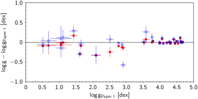
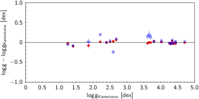
Figure 22: Comparison of our fundamental values of $\log g$ to those determined in Paper I and by Karovicova et al. (2020, 2022a, 2022b). Red dots for SPInS masses using BaSTI models, blue open squares for STAREVOL models.

The final $\log g$ distribution and uncertainties are shown in Fig. 23. The bottom panel shows separately the uncertainties for dwarfs ($\log g$$>$3.8) and giants ($\log g$$\leq$3.8), highlighting the lower precision obtained for giants. The median uncertainty is 0.02 dex for dwarfs and 0.06 dex for giants. While 90% of the dwarfs have an uncertainty lower than 0.05 dex, 90% of the giants have an uncertainty higher than 0.03 dex.

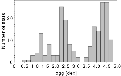
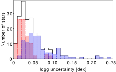
Figure 23: Histogram of $\log g$ (top panel) and uncertainty (bottom panel). The bottom panel shows the uncertainties for dwarfs (red) and giants (blue).

5 The new set of Gaia FGK benchmark stars

The fundamental $T_{\rm eff}$ and $\log g$ determined for the 192 GBS V3 stars with a direct value of $\theta_{\rm LD}$ are given in Table LABEL:t:fund_teff_logg of Appendix A while the nine other stars from V1 and V2 with an indirect $\theta_{\rm LD}$ are provided in Table 3. The metallicity from the literature is provided for convenience, but will be redetermined homogeneously in the coming Paper VIII. The full catalogue with all the other parameters determined in this work is available in VizieR.

Table 3: $T_{\rm eff}$ and $\log g$ determined in this work for stars from V1 and V2 with an indirect value of $\theta_{\rm LD}$. [Fe/H] from the literature is given for indication.

HIP	HD	$T_{\rm eff}$	$\log g$	[Fe/H]
		(K)	(dex)	(dex)
14086	18907	5143$\pm$ 56	3.53$\pm$0.03	-0.63
17147	22879	5962$\pm$ 86	4.28$\pm$0.04	-0.84
48152	84937	6484$\pm$106	4.16$\pm$0.05	-2.12
50382	298986	6343$\pm$ 43	4.29$\pm$0.02	-1.33
57360	102200	6205$\pm$ 45	4.27$\pm$0.02	-1.23
59490	106038	6172$\pm$ 42	4.28$\pm$0.02	-1.33
60172	107328	4576$\pm$ 87	1.77$\pm$0.22	-0.38
86796	160691	5974$\pm$ 60	4.30$\pm$0.03	+0.29
104659	201891	6040$\pm$ 44	4.34$\pm$0.02	-1.02

The Kiel diagram with fundamental $T_{\rm eff}$ and $\log g$ is shown in Fig. 24 for the full sample of 192 stars and for a selection of the best stars, with an uncertainty on $T_{\rm eff}$ and $\log g$ better than 2% and 0.1 dex, respectively. This selection of 165 stars mainly rejects giants with large uncertainties, as discussed in Sect. 4, but still preserves a good distribution across the Kiel diagram.

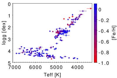
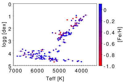
Figure 24: Kiel diagram with fundamental $T_{\rm eff}$ and $\log g$. The colour scale is related to metallicities from the literature. The left panel shows the full sample of 192 stars while the right panel shows the stars with uncertainties on $T_{\rm eff}$ and $\log g$ better than 2% and 0.1 dex respectively.

The metallicity histogram of the GBS V3 is shown in Fig. 25, compared to that of V1 (only considering stars with a direct $\theta_{\rm LD}$), highlighting a number of new metal-poor stars. This is however more evident in the interval $-1.0<$[Fe/H]$<-0.5$ than below [Fe/H]=$-1.0$. There were four stars in GBS V1 with $-1.0<$[Fe/H]$<-0.5$, a number increased to 14 in GBS V3. Four giant stars with [Fe/H]$<-1.0$ were added, which doubles the V1 number of stars with [Fe/H]$<-1.0$. The fundamental $T_{\rm eff}$ and $\log g$ for these eight GBS V3 stars are presented in Table 4 together with the values from Paper I for the four stars in common.

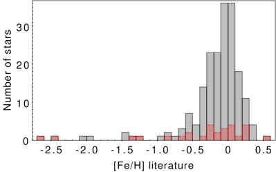
Figure 25: Histogram of [Fe/H] for the 192 fundamental GBS V3 (grey) compared to the V1 version (red).

Table 4: Fundamental $T_{\rm eff}$ and $\log g$ for the eight GBS V3 with [Fe/H]$<-1.0$ (from the literature), and comparison to the Paper I values, when available.

HIP	other name	$T_{\rm eff}$ V3	$T_{\rm eff}$ V1	$\log g$ V3	$\log g$ V1	[Fe/H]
HIP2413	HD2665	4951$\pm$25		2.318$\pm$0.029		-1.97
HIP5445	HD6755	4977$\pm$27		2.767$\pm$0.027		-1.43
HIP8837	$\psi$ Phe	3362$\pm$183	3472$\pm$92	0.438$\pm$0.058	0.51$\pm$0.18	-1.24
HIP57939	HD103095	5235$\pm$18	4827$\pm$55	4.717$\pm$0.014	4.6$\pm$0.03	-1.33
HIP68594	HD122563	4642$\pm$35	4587$\pm$60	1.312$\pm$0.029	1.61$\pm$0.07	-2.67
HIP76976	HD140283	5788$\pm$45	5522$\pm$105	3.750$\pm$0.089	3.58$\pm$0.11	-2.48
HIP92167	HD175305	4902$\pm$30		2.533$\pm$0.017		-1.45
HIP115949	HD221170	4380$\pm$18		1.216$\pm$0.023		-2.10

One of the main purposes of the GBS is to calibrate or validate atmospheric parameters from spectroscopy. We therefore checked spectroscopic $T_{\rm eff}$ and $\log g$ available in different sources, using the subset of 165 most reliable GBS.

Fig. 26 compares our fundamental determinations with those available in the PASTEL catalogue, based on high-resolution, high signal-to-noise spectroscopy. Overall, the agreement on $T_{\rm eff}$ is good with a dispersion of MAD=54 K and a slight offset of 12 K (median), the spectroscopic $T_{\rm eff}$ being larger. Two extreme outliers have differences larger than 400 K. For HIP86614 we suspect an uncertain angular diameter given its noisy squared visibility curve in Boyajian et al. (2012b) while for HIP108535 the only spectroscopic $T_{\rm eff}$ in PASTEL is dubious. For that star we note a good agreement with the determination by Prugniel et al. (2011) based on a medium resolution spectrum.

Concerning $\log g$ we can see three regimes of precision, corresponding to dwarfs, clump giants, and cooler giants, with an increasing dispersion. The dispersion among dwarfs is 0.04 dex (MAD). It rises to 0.1 dex among clump giants (2.0$<$$\log g$$<$3.5) with no offset, while for red giants there is a tendency of spectroscopic $\log g$ to be larger than the fundamental ones by 0.16 dex (median offset) with a significant dispersion of 0.2 dex (MAD). The GBS can therefore be used to better understand and correct the spectroscopic gravities of evolved stars.

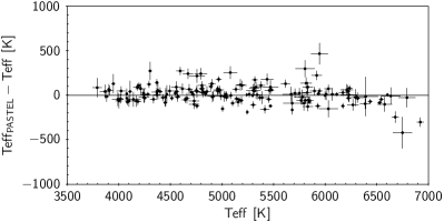
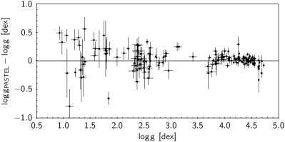
Figure 26: Comparison of our fundamental values of $T_{\rm eff}$ (top panel) and $\log g$ (bottom panel) to spectroscopic ones available in the PASTEL catalogue.

Focusing on the best studied stars we selected in the PASTEL catalogue the stars which are included in at least 15 spectroscopic studies at high resolution and high signal to noise ratio since 1990. The resulting 16 stars are all dwarfs or subgiants, with some of them also in common with Paper I. In general there is a good agreement, within our uncertainties and the standard deviation from the literature values. Three stars, HIP14954, HIP57939 and HIP8159, exhibit a significant difference in $T_{\rm eff}$, larger than 150 K.

HIP14954 (94 Cet) has been very much studied, with 41 spectroscopic determinations of $T_{\rm eff}$, likely because of its exoplanet discovered in 2000 (Queloz et al., 2001). The literature values range from 5916 K to 6424 K with a mean of 6176 K and a standard deviation of 84 K. Our determination is lower, $T_{\rm eff}$=5912$\pm$59 K, but still in agreement with the coolest spectroscopic determinations. Our fundamental value is in a very good agreement with that of Boyajian et al. (2013), $T_{\rm eff}$=5916$\pm$98 K, independent from ours since we use the angular diameter from Ligi et al. (2016). It would be important to better understand why spectroscopy gives a higher $T_{\rm eff}$ for that star because it has implications on the parameters of its exoplanet.

HIP8159 (109 Psc) also hosts an exoplanet and has several recent $T_{\rm eff}$ from high resolution spectroscopy ranging between 5560 K and 5711 K. The fundamental determinations, from Boyajian et al. (2013) and from us ($T_{\rm eff}$=5438$\pm$61 K) based on the same $\theta_{\rm LD}$, are cooler than the mean spectroscopic value by $\sim$200 K. This discrepancy requires further investigation.

HIP57939 (HD103095) has 57 spectroscopic determinations of $T_{\rm eff}$ after 1990, ranging from 4500 K to 5250 K with a mean of 5057 K and a standard deviation of 18 K. Our fundamental determination $T_{\rm eff}$=5235$\pm$18 K is in agreement with the hottest spectroscopic determinations, e.g. by Luck & Heiter (2005).

We also checked atmospheric parameters massively determined by large spectroscopic surveys against our fundamental determinations of the best GBS. We considered APOGEE DR17 (Majewski et al., 2017; Abdurro’uf et al., 2022), the Gaia-ESO survey (Randich et al., 2022; Gilmore et al., 2022) and GALAH DR3 (Buder et al., 2021) in the comparisons shown in Fig. 27. Table 5 gives the median offsets and corresponding MAD for dwarfs and giants separately. Although GALAH and Gaia-ESO have less stars in common than APOGEE, we see the same trends in the three surveys. Their $T_{\rm eff}$ and $\log g$ for dwarfs are smaller on average than the fundamental ones, and vice-versa for the giants. These trends are worth to be investigated and better understood.

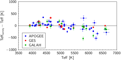
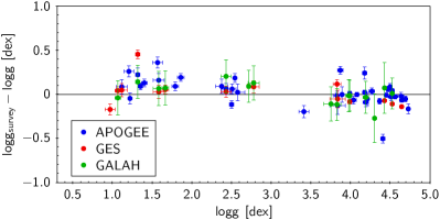
Figure 27: Comparison of $T_{\rm eff}$ and $\log g$ from this work with the spectroscopic ones in surveys: APOGEE DR17 (blue), Gaia-ESO (red), GALAH DR3 (green).

Table 5: Median difference (MED) and median absolute deviation (MAD) between our fundamental determinations of $T_{\rm eff}$ and $\log g$ and the spectroscopic ones from surveys (survey results minus our results), for N stars in common.

Sample	N	$\Delta$$T_{\rm eff}$		$\Delta$$\log g$
		MED	MAD	MED	MAD
APOGEE dwarfs	26	-21	111	-0.02	0.04
APOGEE giants	17	38	42	0.09	0.07
Gaia-ESO dwarfs	6	-52	38	-0.08	0.03
Gaia-ESO giants	9	39	92	0.05	0.02
GALAH dwarfs	7	-119	32	-0.01	0.02
GALAH giants	8	53	73	0.08	0.05

Finally we also assessed the photometric and spectroscopic $T_{\rm eff}$ and $\log g$ of the Gaia DR3 Golden Sample of Astrophysical Parameters (Gaia Collaboration et al., 2023a) with the best GBS, as shown in Fig. 28. Photometric $T_{\rm eff}$ are lower than fundamental ones by 58 K, while the offset of the spectroscopic $T_{\rm eff}$ is negligible (6 K). For $\log g$ there is an excellent agreement of the photometric values with median offset of $-0.03$ dex and a dispersion (MAD) of 0.06 dex. Spectroscopic $\log g$, corrected as suggested by Recio-Blanco et al. (2023), are found smaller than the fundamental values by 0.06 dex, with a dispersion of 0.15 dex. These comparisons are based on 35 and 38 stars in common for the photometric and spectroscopic parameters respectively, mainly dwarfs.

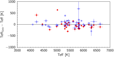
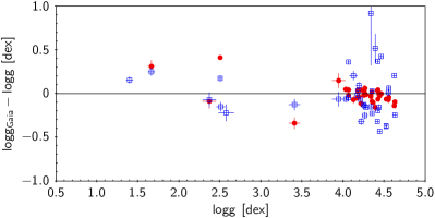
Figure 28: Comparison of $T_{\rm eff}$ and $\log g$ from this work with the photometric (red dots) and spectroscopic (blue squares) ones from the Gaia DR3 Golden Sample of Astrophysical Parameters (Gaia Collaboration et al., 2023a).

6 Conclusion

Large spectroscopic surveys usually calibrate or validate their determinations of atmospheric parameters using reference stars. Ideally they should adopt a common $T_{\rm eff}$ and $\log g$ scale in order to minimize systematic differences in abundances provided by different instruments and pipelines. The GBS are intended to provide such an anchor to the fundamental $T_{\rm eff}$ and $\log g$. GBS are also suited to help understand any shortcomings in the stellar models.

We have presented determinations of fundamental $T_{\rm eff}$ and $\log g$, based on the Stefan-Boltzmann law and Newton’s law of gravitation, for the third version of the GBS. Compared to the previous V1 and V2 versions, a significant improvement is the larger number of stars, 192 instead of $\sim$40, resulting from our systematic search of high quality angular diameters based on interferometric measurements. More accurate $\log g$ were obtained thanks to the higher precision parallaxes which mostly come from Gaia DR3, while the improved $T_{\rm eff}$ are in part a result of the homogenous photometric data from Gaia DR3, which feed into the $F_{\rm bol}$ determination. $F_{\rm bol}$ are now more precise and homogeneous owing to the methodology of SED fitting applied to a combination of photometric and spectrophotometric data including measurements made on BP/RP spectra from Gaia DR3. Better $F_{\rm bol}$ also result from the adopted extinction values deduced from state-fo-the-art 3D maps of the solar neighbourhood. The most difficult part comes from the determination of masses from evolutionary tracks. We have shown that using two different grids can lead to differences of up to more than 50% in masses, giving systematic offsets of about 0.06 dex in $\log g$ among giants.

At each stage of the compilation and determination of the parameters, we evaluated the uncertainties that we aimed to keep at the 1-2% level. Our results were assessed by comparing them to other determinations of similar accuracy available in the literature. In general the comparison with literature data is satisfactory, with differences not exceeding 4%. We can explain most of the outliers. We also determined seismic radii, masses and surface gravities for comparisons, using scaling relations and seismic parameters available for $\sim$40 stars. They show a good agreement for dwarfs but a trend in masses outside the 1-1.5M_⊙ range. From the different comparisons we are confident that our uncertainties in $T_{\rm eff}$ are reliable. We reach the expected 1-2% level in $T_{\rm eff}$. For $\log g$ only dwarfs have such a level of accuracy. Uncertainties for giants are larger and reflect the difficulty to obtain reliable masses for them from evolutionary tracks.

The $T_{\rm eff}$ and $\log g$ presented here will be updated. Two steps of our determination process, $F_{\rm bol}$ and masses, depend on [Fe/H] which we took from the literature. This is the subject of the coming paper VIII to determine abundances of the GBS-V3 from a large collection of high quality spectra. Some iterations will be needed to adjust $T_{\rm eff}$, $\log g$ and [Fe/H] in a self-consistent way. In the meantime, we have evaluated the impact of using non-homogeneous metallicities through tests in which we modified the values of [Fe/H] and uncertainties by 0.15 dex in input of the SED fitting and of SPInS. We found that it has a negligible impact on $T_{\rm eff}$, and also on $\log g$ for most of the stars, although a few giants have their mass affected by more than 30% inducing a change of $\log g$ by 0.11 to 0.5 dex.

In order to use the GBS V3 for calibration or validation of atmospheric parameters, we recommend the users to select the 165 stars with uncertainties on $T_{\rm eff}$ and $\log g$ lower than 2% and 0.1 dex, respectively. We have used this subsample to assess $T_{\rm eff}$ and $\log g$ obtained by high-resolution and high-signal to noise spectroscopy (PASTEL catalogue), by medium-resolution spectroscopy (APOGEE, GALAH and Gaia-ESO surveys), and by Gaia photometry and spectroscopy. This has revealed some issues that need to be investigated to improve the future releases.

Due to the lack of metal-poor stars in the solar neighbourhood the GBS V3 do not yet cover the metallicity range in a uniform way. We still lack angular diameters for stars with [Fe/H]$<-1.0$ which are important targets in galactic archeology and stellar physics. Interferometric measurements are still limited to stars brighter than V$\sim$8, and larger than $\theta_{\rm LD}$$\simeq$0.2 mas. There are however metal-poor candidates which are bright and large enough to fulfil these criteria. They could be observed with powerful interferometers, such as the new SPICA instrument on the CHARA array (Mourard et al., 2022) expected to provide an estimation of the stellar radius of such stars to 1% precision. It would also be useful to remeasure partly or totally the GBS with $\theta_{\rm LD}$$<$1.2 mas, which show a large dispersion of the current measurements, exceeding the quoted uncertainties.

Appendix A Table with $T_{\rm eff}$ and $\log g$ of the GBS V3

Table 6: Fundamental $T_{\rm eff}$ and $\log g$ and their uncertainties determined in this work for the 192 GBS V3, with [Fe/H] from the literature and the $\theta_{\rm LD}$ adopted measurement.

HIP	HD	$\theta_{\rm LD}$	Reference for $\theta_{\rm LD}$	$T_{\rm eff}$	ru_$T_{\rm eff}$	$\log g$	[Fe/H]
		(mas)		(K)	(%)	(dex)	(dex)
HIP101345	HD195564	0.712 $\pm$ 0.03	2013ApJ…771…40B	5514 $\pm$ 116	2.1	3.95 $\pm$ 0.09	0.05
HIP10234	HD13468	0.886 $\pm$ 0.01	2018A&A…616A..68G	4676 $\pm$ 80	1.7	2.37 $\pm$ 0.09	-0.13
HIP102422	HD198149	2.882 $\pm$ 0.088	2016ApJS..227….4H	4751 $\pm$ 73	1.5	3.15 $\pm$ 0.05	-0.13
HIP103598	HD200205	2.032 $\pm$ 0.043	2010ApJ…710.1365B	4032 $\pm$ 45	1.1	1.20 $\pm$ 0.06	-0.36
HIP104214	HD201091	1.775 $\pm$ 0.013	2008A&A…488..667K	4398 $\pm$ 34	0.8	4.63 $\pm$ 0.01	-0.13
HIP104217	HD201092	1.581 $\pm$ 0.022	2008A&A…488..667K	4174 $\pm$ 47	1.1	4.68 $\pm$ 0.02	-0.21
HIP106039	HD204381	1.524 $\pm$ 0.017	2018A&A…616A..68G	5079 $\pm$ 31	0.6	2.86 $\pm$ 0.04	-0.11
HIP108535	HD209369	0.621 $\pm$ 0.017	2016A&A…586A..94L	6754 $\pm$ 93	1.4	3.84 $\pm$ 0.05	-0.24
HIP108870	HD209100	1.758 $\pm$ 0.012	2020MNRAS.493.2377R	4754 $\pm$ 35	0.7	4.62 $\pm$ 0.01	-0.13
HIP109176	HD210027	1.206 $\pm$ 0.053	2009ApJ…694.1085V	6419 $\pm$ 141	2.2	4.15 $\pm$ 0.06	-0.11
HIP109937	HD211388	3.371 $\pm$ 0.049	2018AJ….155…30B	4258 $\pm$ 41	1.0	1.39 $\pm$ 0.05	-0.05
HIP11095	HD15248	0.949 $\pm$ 0.019	2018A&A…616A..68G	4721 $\pm$ 52	1.1	2.59 $\pm$ 0.06	0.06
HIP111944	HD214868	2.731 $\pm$ 0.02	2010ApJ…710.1365B	4203 $\pm$ 34	0.8	1.56 $\pm$ 0.06	-0.20
HIP112440	HD215665	2.26 $\pm$ 0.1	1999AJ….118.3032N	4848 $\pm$ 109	2.2	2.12 $\pm$ 0.08	-0.07
HIP112447	HD215648	1.091 $\pm$ 0.008	2012ApJ…746..101B	6223 $\pm$ 23	0.4	3.95 $\pm$ 0.04	-0.27
HIP112731	HD216174	1.5980 $\pm$ 0.0120	2016AJ….152…66B	4297 $\pm$ 36	0.8	1.75 $\pm$ 0.03	-0.55
HIP112748	HD216131	2.496 $\pm$ 0.04	2003AJ….126.2502M	4961 $\pm$ 40	0.8	2.85 $\pm$ 0.03	-0.03
HIP113357	HD217014	0.685 $\pm$ 0.011	2013ApJ…771…40B	5746 $\pm$ 72	1.3	4.33 $\pm$ 0.02	0.18
HIP114622	HD219134	1.106 $\pm$ 0.007	2012ApJ…757..112B	4800 $\pm$ 34	0.7	4.55 $\pm$ 0.01	0.06
HIP114855	HD219449	2.22 $\pm$ 0.031	2018AJ….155…30B	4631 $\pm$ 69	1.5	2.32 $\pm$ 0.11	-0.03
HIP114971	HD219615	2.3400 $\pm$ 0.0400	2015A&A…573A.138B	4970 $\pm$ 43	0.9	2.44 $\pm$ 0.12	-0.53
HIP115227	HD220009	2.045 $\pm$ 0.034	2015A&A…582A..49H	4227 $\pm$ 77	1.8	1.66 $\pm$ 0.04	-0.66
HIP115620	HD220572	1.092 $\pm$ 0.013	2018A&A…616A..68G	4756 $\pm$ 41	0.9	2.61 $\pm$ 0.06	0.08
HIP115949	HD221170	0.596 $\pm$ 0.005	2020A&A…640A..25K	4380 $\pm$ 19	0.4	1.22 $\pm$ 0.02	-2.10
HIP116771	HD222368	1.082 $\pm$ 0.009	2012ApJ…746..101B	6169 $\pm$ 56	0.9	4.09 $\pm$ 0.02	-0.14
HIP12114	HD16160	1.03 $\pm$ 0.007	2012ApJ…757..112B	4583 $\pm$ 76	1.6	4.52 $\pm$ 0.01	-0.13
HIP12486	HD16815	2.248 $\pm$ 0.014	2018A&A…616A..68G	4720 $\pm$ 23	0.5	2.37 $\pm$ 0.06	-0.36
HIP12530	HD16765A	0.497 $\pm$ 0.007	2013ApJ…771…40B	6310 $\pm$ 51	0.8	4.36 $\pm$ 0.02	-0.02
HIP12777	HD16895	1.103 $\pm$ 0.008	2012ApJ…746..101B	6206 $\pm$ 23	0.4	4.26 $\pm$ 0.01	0.01
HIP13288	HD17824	1.391 $\pm$ 0.015	2018A&A…616A..68G	4980 $\pm$ 64	1.3	2.89 $\pm$ 0.03	-0.02
HIP13328	HD17709	4.056 $\pm$ 0.041	2003AJ….126.2502M	3799 $\pm$ 72	1.9	0.93 $\pm$ 0.06	-0.36
HIP14060	HD18784	1.036 $\pm$ 0.014	2018A&A…616A..68G	4652 $\pm$ 80	1.7	2.30 $\pm$ 0.12	0.00
HIP14135	HD18884	12.2 $\pm$ 0.04	2006A&A…460..855W	3738 $\pm$ 170	4.5	0.66 $\pm$ 0.07	-0.24
HIP14632	HD19373	1.246 $\pm$ 0.007	2012ApJ…746..101B	5921 $\pm$ 17	0.3	4.17 $\pm$ 0.01	0.09
HIP14838	HD19787	1.87 $\pm$ 0.12	1999AJ….118.3032N	4703 $\pm$ 161	3.4	2.36 $\pm$ 0.23	0.11
HIP14954	HD19994	0.761 $\pm$ 0.01	2016A&A…586A..94L	5912 $\pm$ 59	1.0	4.00 $\pm$ 0.04	0.20
HIP15457	HD20630	0.936 $\pm$ 0.024	2012ApJ…746..101B	5786 $\pm$ 87	1.5	4.50 $\pm$ 0.04	0.04
HIP15776	HD21019	0.606 $\pm$ 0.015	2013ApJ…771…40B	5259 $\pm$ 66	1.3	3.73 $\pm$ 0.12	-0.45
HIP16537	HD22049	2.087 $\pm$ 0.011	2020MNRAS.493.2377R	5130 $\pm$ 30	0.6	4.63 $\pm$ 0.01	-0.08
HIP16852	HD22484	1.081 $\pm$ 0.014	2012ApJ…746..101B	6000 $\pm$ 59	1.0	4.06 $\pm$ 0.03	-0.08
HIP1686	HD1671	0.6 $\pm$ 0.006	2016A&A…586A..94L	6674 $\pm$ 34	0.5	3.69 $\pm$ 0.04	-0.09
HIP17086	HD22798	0.792 $\pm$ 0.021	2020A&A…639A..67N	4652 $\pm$ 88	1.9	2.40 $\pm$ 0.25	0.24
HIP171	HD224930	0.716 $\pm$ 0.007	2020A&A…640A..25K	5445 $\pm$ 30	0.6	4.39 $\pm$ 0.03	-0.79
HIP17378	HD23249	2.343 $\pm$ 0.009	2020MNRAS.493.2377R	5026 $\pm$ 38	0.8	3.83 $\pm$ 0.10	0.09
HIP17595	HD23526	0.915 $\pm$ 0.021	2018A&A…616A..68G	4763 $\pm$ 81	1.7	2.33 $\pm$ 0.15	-0.15
HIP17738	HD23940	1.093 $\pm$ 0.021	2018A&A…616A..68G	4815 $\pm$ 52	1.1	2.43 $\pm$ 0.06	-0.34
HIP18859	HD25457	0.582 $\pm$ 0.016	2018ApJ…858…71S	6295 $\pm$ 91	1.5	4.39 $\pm$ 0.04	0.10
HIP19849		1.504 $\pm$ 0.006	2012ApJ…757..112B	5181 $\pm$ 21	0.4	4.51 $\pm$ 0.01	-0.29
HIP2021	HD2151	2.257 $\pm$ 0.019	2007MNRAS.380L..80N	5917 $\pm$ 25	0.4	3.97 $\pm$ 0.04	-0.12
HIP21421	HD29139	20.58 $\pm$ 0.03	2005A&A…433..305R	3921 $\pm$ 80	2.0	1.17 $\pm$ 0.05	-0.20
HIP22449	HD30652	1.526 $\pm$ 0.004	2012ApJ…746..101B	6518 $\pm$ 35	0.5	4.31 $\pm$ 0.01	0.03
HIP22453	HD30504	2.803 $\pm$ 0.013	2009MNRAS.394.1925V	4097 $\pm$ 20	0.5	1.32 $\pm$ 0.05	-0.34
HIP22479	HD30814	1.31 $\pm$ 0.01	2018A&A…616A..68G	4901 $\pm$ 27	0.6	2.73 $\pm$ 0.04	-0.02
HIP2413	HD2665	0.395 $\pm$ 0.004	2020A&A…640A..25K	4951 $\pm$ 25	0.5	2.32 $\pm$ 0.03	-1.97
HIP24813	HD34411	0.981 $\pm$ 0.015	2012ApJ…746..101B	5823 $\pm$ 45	0.8	4.20 $\pm$ 0.02	0.06
HIP25993	HD36848	1.386 $\pm$ 0.098	2012A&A…539A..58C	4537 $\pm$ 163	3.6	2.71 $\pm$ 0.13	0.19
HIP26019	HD36874	1.118 $\pm$ 0.011	2018A&A…616A..68G	4616 $\pm$ 32	0.7	2.47 $\pm$ 0.10	0.00
HIP27435	HD38858	0.572 $\pm$ 0.009	2013ApJ…771…40B	5705 $\pm$ 47	0.8	4.43 $\pm$ 0.02	-0.22
HIP27530	HD39523	1.939 $\pm$ 0.016	2018A&A…616A..68G	4583 $\pm$ 80	1.7	2.36 $\pm$ 0.13	0.15
HIP27621	HD39640	1.251 $\pm$ 0.017	2018A&A…616A..68G	4851 $\pm$ 41	0.8	2.60 $\pm$ 0.05	-0.11
HIP27913	HD39587	1.051 $\pm$ 0.009	2012ApJ…746..101B	5883 $\pm$ 63	1.1	4.47 $\pm$ 0.02	-0.03
HIP28011	HD39910	1.09 $\pm$ 0.008	2018A&A…616A..68G	4565 $\pm$ 33	0.7	2.50 $\pm$ 0.05	0.26
HIP28139	HD40020	1.012 $\pm$ 0.023	2018A&A…616A..68G	4671 $\pm$ 59	1.3	2.57 $\pm$ 0.09	0.13
HIP29575	HD43023	0.842 $\pm$ 0.014	2020A&A…639A..67N	5043 $\pm$ 43	0.9	2.96 $\pm$ 0.08	0.00
HIP3031	HD3546	1.77 $\pm$ 0.08	1999AJ….118.3032N	4909 $\pm$ 111	2.3	2.44 $\pm$ 0.11	-0.62
HIP30565	HD46116	1.145 $\pm$ 0.031	2018A&A…616A..68G	4880 $\pm$ 68	1.4	2.53 $\pm$ 0.15	-0.32
HIP3093	HD3651	0.722 $\pm$ 0.007	2016A&A…586A..94L	5297 $\pm$ 31	0.6	4.52 $\pm$ 0.02	0.14
HIP3137	HD3750	1.003 $\pm$ 0.02	2018A&A…616A..68G	4610 $\pm$ 51	1.1	2.40 $\pm$ 0.13	0.03
HIP32362	HD48737	1.401 $\pm$ 0.009	2012ApJ…746..101B	6537 $\pm$ 25	0.4	3.79 $\pm$ 0.03	0.14
HIP32851	HD49933A	0.445 $\pm$ 0.012	2011A&A…534L…3B	6628 $\pm$ 89	1.3	4.19 $\pm$ 0.04	-0.39
HIP3456	HD4211	1.1 $\pm$ 0.011	2018A&A…616A..68G	4572 $\pm$ 35	0.8	2.34 $\pm$ 0.10	0.01
HIP36444	HD60060	0.948 $\pm$ 0.01	2018A&A…616A..68G	4814 $\pm$ 32	0.7	2.59 $\pm$ 0.04	-0.08
HIP36732	HD60341	1.19 $\pm$ 0.022	2018A&A…616A..68G	4563 $\pm$ 53	1.2	2.40 $\pm$ 0.08	0.01
HIP37279	HD61421	5.406 $\pm$ 0.006	2021AJ….162..198B	6582 $\pm$ 5	0.1	3.98 $\pm$ 0.02	-0.02
HIP3765	HD4628	0.868 $\pm$ 0.004	2012ApJ…757..112B	5093 $\pm$ 33	0.6	4.64 $\pm$ 0.01	-0.26
HIP37664	HD62713	1.446 $\pm$ 0.012	2018A&A…616A..68G	4661 $\pm$ 32	0.7	2.29 $\pm$ 0.08	0.02
HIP37826	HD62509	8.018 $\pm$ 0.043	2016ApJS..227….4H	4810 $\pm$ 14	0.3	2.55 $\pm$ 0.03	0.02
HIP3850	HD4747	0.39 $\pm$ 0.007	2019ApJ…873…83W	5351 $\pm$ 48	0.9	4.55 $\pm$ 0.03	-0.23
HIP40526	HD69267	5.03 $\pm$ 0.03	1999AJ….118.3032N	4080 $\pm$ 15	0.4	1.28 $\pm$ 0.05	-0.20
HIP40693	HD69830	0.674 $\pm$ 0.014	2015ApJ…800..115T	5317 $\pm$ 58	1.1	4.45 $\pm$ 0.03	-0.03
HIP40843	HD69897	0.706 $\pm$ 0.013	2013ApJ…771…40B	6203 $\pm$ 57	0.9	4.17 $\pm$ 0.02	-0.28
HIP4151	HD5015	0.865 $\pm$ 0.01	2012ApJ…746..101B	6033 $\pm$ 37	0.6	4.03 $\pm$ 0.03	0.05
HIP4257	HD5268	0.767 $\pm$ 0.035	2020A&A…639A..67N	4944 $\pm$ 116	2.3	2.36 $\pm$ 0.18	-0.35
HIP43587	HD75732	0.724 $\pm$ 0.011	2016A&A…586A..94L	5169 $\pm$ 44	0.8	4.41 $\pm$ 0.02	0.32
HIP43813	HD76294	3.196 $\pm$ 0.017	2018AJ….155…30B	4836 $\pm$ 14	0.3	2.49 $\pm$ 0.04	-0.05
HIP45343	HD79210	0.871 $\pm$ 0.014	2012ApJ…757..112B	3997 $\pm$ 34	0.9	4.69 $\pm$ 0.02	0.17
HIP45860	HD80493	7.538 $\pm$ 0.075	2003AJ….126.2502M	3881 $\pm$ 20	0.5	1.06 $\pm$ 0.04	-0.26
HIP4587	HD5722	0.995 $\pm$ 0.019	2018A&A…616A..68G	4914 $\pm$ 50	1.0	2.61 $\pm$ 0.05	-0.23
HIP46853	HD82328	1.632 $\pm$ 0.005	2012ApJ…746..101B	6217 $\pm$ 44	0.7	3.83 $\pm$ 0.05	-0.17
HIP47080	HD82885	0.821 $\pm$ 0.012	2012ApJ…746..101B	5452 $\pm$ 46	0.8	4.44 $\pm$ 0.02	0.34
HIP47431	HD83618	3.462 $\pm$ 0.033	2018AJ….155…30B	4238 $\pm$ 22	0.5	1.78 $\pm$ 0.04	-0.06
HIP47908	HD84441	2.643 $\pm$ 0.015	2009MNRAS.394.1925V	5314 $\pm$ 17	0.3	2.36 $\pm$ 0.05	-0.03
HIP48455	HD85503	2.887 $\pm$ 0.016	2018AJ….155…30B	4519 $\pm$ 23	0.5	2.43 $\pm$ 0.06	0.27
HIP49081	HD86728	0.771 $\pm$ 0.012	2012ApJ…746..101B	5610 $\pm$ 46	0.8	4.25 $\pm$ 0.02	0.20
HIP49637	HD87837	3.33 $\pm$ 0.04	1999AJ….118.3032N	4106 $\pm$ 47	1.2	1.59 $\pm$ 0.06	-0.02
HIP49908	HD88230	1.268 $\pm$ 0.04	2001ApJ…551L..81L	4132 $\pm$ 72	1.7	4.63 $\pm$ 0.04	0.21
HIP50564	HD89449	0.731 $\pm$ 0.026	2013MNRAS.434.1321M	6385 $\pm$ 120	1.9	4.12 $\pm$ 0.05	0.10
HIP50887	HD90043	0.659 $\pm$ 0.009	2018MNRAS.477.4403W	4801 $\pm$ 83	1.7	3.11 $\pm$ 0.06	-0.03
HIP51459	HD90839	0.794 $\pm$ 0.014	2012ApJ…746..101B	6259 $\pm$ 56	0.9	4.40 $\pm$ 0.02	-0.12
HIP5336	HD6582	0.973 $\pm$ 0.009	2008ApJ…683..424B	5358 $\pm$ 31	0.6	4.49 $\pm$ 0.01	-0.83
HIP544	HD166	0.624 $\pm$ 0.009	2013ApJ…771…40B	5378 $\pm$ 40	0.7	4.46 $\pm$ 0.02	0.11
HIP5445	HD6755	0.369 $\pm$ 0.004	2020A&A…640A..25K	4977 $\pm$ 27	0.5	2.77 $\pm$ 0.03	-1.43
HIP54539	HD96833	4.131 $\pm$ 0.007	2018AJ….155…30B	4543 $\pm$ 6	0.1	2.12 $\pm$ 0.05	-0.11
HIP5458	HD6833	0.852 $\pm$ 0.008	2020A&A…640A..25K	4447 $\pm$ 42	0.9	1.83 $\pm$ 0.02	-0.86
HIP55219	HD98262	4.561 $\pm$ 0.016	2018AJ….155…30B	4187 $\pm$ 61	1.4	1.38 $\pm$ 0.10	-0.14
HIP56127	HD99998	3.21 $\pm$ 0.02	1999AJ….118.3032N	3852 $\pm$ 90	2.3	0.95 $\pm$ 0.06	-0.39
HIP56343	HD100407	2.386 $\pm$ 0.021	2005A&A…436..253T	5034 $\pm$ 34	0.7	2.78 $\pm$ 0.07	-0.09
HIP56997	HD101501	0.91 $\pm$ 0.009	2012ApJ…746..101B	5310 $\pm$ 28	0.5	4.42 $\pm$ 0.01	-0.05
HIP57477	HD102328	1.606 $\pm$ 0.006	2010ApJ…710.1365B	4450 $\pm$ 31	0.7	2.37 $\pm$ 0.08	0.19
HIP57757	HD102870	1.431 $\pm$ 0.006	2012ApJ…746..101B	6093 $\pm$ 13	0.2	4.08 $\pm$ 0.02	0.13
HIP57939	HD103095	0.593 $\pm$ 0.004	2020A&A…640A..25K	5235 $\pm$ 18	0.3	4.72 $\pm$ 0.01	-1.33
HIP61317	HD109358	1.133 $\pm$ 0.034	2018AJ….155…30B	6013 $\pm$ 91	1.5	4.41 $\pm$ 0.04	-0.20
HIP63584	HD113337	0.386 $\pm$ 0.009	2019A&A…627A..44B	6783 $\pm$ 79	1.2	4.24 $\pm$ 0.03	0.17
HIP63608	HD113226	3.318 $\pm$ 0.013	2018AJ….155…30B	4950 $\pm$ 10	0.2	2.72 $\pm$ 0.02	0.06
HIP64394	HD114710	1.127 $\pm$ 0.011	2012ApJ…746..101B	5930 $\pm$ 30	0.5	4.37 $\pm$ 0.01	0.06
HIP65721	HD117176	0.998 $\pm$ 0.004	2015ApJ…806…60K	5473 $\pm$ 22	0.4	3.94 $\pm$ 0.08	-0.06
HIP6592	HD8651	1.228 $\pm$ 0.013	2018A&A…616A..68G	4685 $\pm$ 43	0.9	2.39 $\pm$ 0.08	-0.20
HIP671	HD360	0.906 $\pm$ 0.015	2018A&A…616A..68G	4679 $\pm$ 79	1.7	2.32 $\pm$ 0.11	-0.09
HIP67459	HD120477	4.72 $\pm$ 0.04	1999AJ….118.3032N	3950 $\pm$ 20	0.5	1.30 $\pm$ 0.05	-0.40
HIP67927	HD121370	2.134 $\pm$ 0.012	2014ApJ…781…90B	6161 $\pm$ 18	0.3	3.82 $\pm$ 0.05	0.25
HIP68594	HD122563	0.925 $\pm$ 0.011	2020A&A…640A..25K	4642 $\pm$ 35	0.8	1.32 $\pm$ 0.03	-2.67
HIP69673	HD124897	21.05 $\pm$ 0.21	2008A&A…485..561L	4277 $\pm$ 23	0.5	1.58 $\pm$ 0.07	-0.55
HIP70497	HD126660	1.109 $\pm$ 0.007	2012ApJ…746..101B	6292 $\pm$ 20	0.3	4.06 $\pm$ 0.02	-0.03
HIP70791	HD127243	0.971 $\pm$ 0.007	2020A&A…640A..25K	5015 $\pm$ 23	0.5	2.50 $\pm$ 0.02	-0.70
HIP7083	HD9362	2.301 $\pm$ 0.021	2018A&A…616A..68G	4750 $\pm$ 28	0.6	2.40 $\pm$ 0.05	-0.31
HIP71053	HD127665	3.901 $\pm$ 0.008	2018AJ….155…30B	4181 $\pm$ 56	1.3	1.80 $\pm$ 0.05	-0.17
HIP71681	HD128621	5.999 $\pm$ 0.025	2017A&A…597A.137K	5207 $\pm$ 12	0.2	4.53 $\pm$ 0.01	0.24
HIP71683	HD128620	8.502 $\pm$ 0.038	2017A&A…597A.137K	5804 $\pm$ 13	0.2	4.29 $\pm$ 0.01	0.20
HIP72567	HD130948	0.569 $\pm$ 0.011	2013ApJ…771…40B	5812 $\pm$ 57	1.0	4.33 $\pm$ 0.03	-0.01
HIP7294	HD9408	1.64 $\pm$ 0.09	1999AJ….118.3032N	4774 $\pm$ 131	2.7	2.35 $\pm$ 0.11	-0.30
HIP73184	HD131977	1.098 $\pm$ 0.014	2020MNRAS.493.2377R	4724 $\pm$ 71	1.5	4.63 $\pm$ 0.02	0.02
HIP73568	HD133124	3.055 $\pm$ 0.077	2018AJ….155…30B	3994 $\pm$ 56	1.4	1.37 $\pm$ 0.06	-0.10
HIP74666	HD135722	2.764 $\pm$ 0.03	2003AJ….126.2502M	4810 $\pm$ 30	0.6	2.38 $\pm$ 0.09	-0.35
HIP74793	HD136726	2.149 $\pm$ 0.023	2018AJ….155…30B	4253 $\pm$ 25	0.6	1.78 $\pm$ 0.04	-0.02
HIP74975	HD136202	0.785 $\pm$ 0.023	2013ApJ…771…40B	5820 $\pm$ 99	1.7	3.87 $\pm$ 0.04	-0.02
HIP7607	HD9927	3.649 $\pm$ 0.007	2018AJ….155…30B	4356 $\pm$ 56	1.3	1.99 $\pm$ 0.07	0.05
HIP7643	HD10142	0.964 $\pm$ 0.006	2018A&A…616A..68G	4705 $\pm$ 28	0.6	2.38 $\pm$ 0.10	-0.13
HIP76976	HD140283	0.327 $\pm$ 0.005	2018MNRAS.475L..81K	5788 $\pm$ 45	0.8	3.75 $\pm$ 0.09	-2.48
HIP77052	HD140538	0.597 $\pm$ 0.015	2013ApJ…771…40B	5667 $\pm$ 91	1.6	4.47 $\pm$ 0.04	0.05
HIP78072	HD142860	1.217 $\pm$ 0.005	2012ApJ…746..101B	6296 $\pm$ 16	0.2	4.16 $\pm$ 0.01	-0.18
HIP79672	HD146233	0.676 $\pm$ 0.006	2011A&A…526L…4B	5824 $\pm$ 30	0.5	4.42 $\pm$ 0.01	0.03
HIP7981	HD10476	1.0 $\pm$ 0.004	2013ApJ…771…40B	5129 $\pm$ 71	1.4	4.52 $\pm$ 0.01	-0.04
HIP80843	HD148897	1.917 $\pm$ 0.045	2021ApJ…922..163V	4227 $\pm$ 51	1.2	1.11 $\pm$ 0.07	-0.92
HIP8102	HD10700	2.005 $\pm$ 0.011	2020MNRAS.493.2377R	5463 $\pm$ 16	0.3	4.52 $\pm$ 0.01	-0.51
HIP81300	HD149661	0.724 $\pm$ 0.011	2012ApJ…757..112B	5408 $\pm$ 47	0.9	4.62 $\pm$ 0.02	0.03
HIP8159	HD10697	0.547 $\pm$ 0.012	2013ApJ…771…40B	5438 $\pm$ 61	1.1	3.94 $\pm$ 0.08	0.14
HIP81693	HD150680	2.367 $\pm$ 0.051	2003AJ….126.2502M	5760 $\pm$ 96	1.7	3.72 $\pm$ 0.03	0.03
HIP83000	HD153210	3.608 $\pm$ 0.041	2016ApJS..227….4H	4499 $\pm$ 68	1.5	2.49 $\pm$ 0.07	0.02
HIP8362	HD10780	0.763 $\pm$ 0.018	2012ApJ…746..101B	5293 $\pm$ 77	1.5	4.55 $\pm$ 0.03	0.03
HIP8404	HD11037	0.89 $\pm$ 0.019	2020A&A…639A..67N	4834 $\pm$ 59	1.2	2.33 $\pm$ 0.21	-0.13
HIP84862	HD157214	0.725 $\pm$ 0.012	2013ApJ…771…40B	5825 $\pm$ 49	0.8	4.26 $\pm$ 0.03	-0.39
HIP84950	HD157681	1.908 $\pm$ 0.013	2016AJ….152…66B	4108 $\pm$ 23	0.6	1.35 $\pm$ 0.03	-0.23
HIP85235	HD158633	0.573 $\pm$ 0.01	2013ApJ…771…40B	5188 $\pm$ 51	1.0	4.51 $\pm$ 0.02	-0.46
HIP85258	HD157244	5.997 $\pm$ 0.037	2015A&A…582A..49H	4232 $\pm$ 17	0.4	0.97 $\pm$ 0.06	0.50
HIP86614	HD162003	0.949 $\pm$ 0.025	2012ApJ…746..101B	5936 $\pm$ 89	1.5	3.82 $\pm$ 0.04	0.01
HIP86742	HD161096	4.498 $\pm$ 0.032	2016ApJS..227….4H	4577 $\pm$ 18	0.4	2.33 $\pm$ 0.07	0.06
HIP86974	HD161797	1.88 $\pm$ 0.008	2018AJ….155…30B	5665 $\pm$ 16	0.3	4.05 $\pm$ 0.04	0.25
HIP87808	HD163770	3.15 $\pm$ 0.003	2009MNRAS.394.1925V	4448 $\pm$ 23	0.5	1.37 $\pm$ 0.04	-0.03
HIP87833	HD164058	9.86 $\pm$ 0.128	2003AJ….126.2502M	4018 $\pm$ 32	0.8	1.33 $\pm$ 0.04	-0.08
HIP88348	HD164922	0.4120 $\pm$ 0.0100	2016ApJ…830…46F	5392 $\pm$ 66	1.2	4.43 $\pm$ 0.03	0.18
HIP8837	HD11695	8.13 $\pm$ 0.2	2004A&A…413..711W	3362 $\pm$ 183	5.4	0.44 $\pm$ 0.06	-1.24
HIP89047	HD167042	0.831 $\pm$ 0.0068	2020A&A…640A…2S	4987 $\pm$ 66	1.3	3.41 $\pm$ 0.06	0.04
HIP8928	HD11977	1.528 $\pm$ 0.013	2018A&A…616A..68G	4890 $\pm$ 30	0.6	2.61 $\pm$ 0.05	-0.15
HIP89348	HD168151	0.664 $\pm$ 0.014	2016A&A…586A..94L	6569 $\pm$ 69	1.1	4.09 $\pm$ 0.03	-0.29
HIP89962	HD168723	3.062 $\pm$ 0.048	2016ApJS..227….4H	4801 $\pm$ 47	1.0	2.92 $\pm$ 0.04	-0.20
HIP90344	HD170693	2.041 $\pm$ 0.043	2010ApJ…710.1365B	4367 $\pm$ 46	1.1	1.86 $\pm$ 0.04	-0.45
HIP9094	HD11964	0.607 $\pm$ 0.015	2013ApJ…771…40B	5082 $\pm$ 63	1.2	3.88 $\pm$ 0.08	0.11
HIP91949	HD173701	0.332 $\pm$ 0.006	2012ApJ…760…32H	5315 $\pm$ 48	0.9	4.44 $\pm$ 0.03	0.30
HIP92043	HD173667	1.0 $\pm$ 0.006	2012ApJ…746..101B	6426 $\pm$ 20	0.3	3.95 $\pm$ 0.03	-0.04
HIP92167	HD175305	0.484 $\pm$ 0.006	2020A&A…640A..25K	4902 $\pm$ 30	0.6	2.53 $\pm$ 0.02	-1.45
HIP92512	HD175306	2.189 $\pm$ 0.007	2015ApJ…809..159R	4464 $\pm$ 23	0.5	1.78 $\pm$ 0.06	-0.53
HIP92984	HD175726	0.346 $\pm$ 0.007	2012ApJ…760…32H	6070 $\pm$ 62	1.0	4.48 $\pm$ 0.03	-0.04
HIP93427	HD177153	0.2890 $\pm$ 0.0060	2012ApJ…760…32H	6016 $\pm$ 63	1.0	4.24 $\pm$ 0.03	-0.05
HIP93429	HD176678	2.463 $\pm$ 0.012	2018AJ….155…30B	4491 $\pm$ 105	2.3	2.31 $\pm$ 0.11	-0.08
HIP9440	HD12438	1.091 $\pm$ 0.016	2018A&A…616A..68G	4954 $\pm$ 42	0.8	2.45 $\pm$ 0.08	-0.58
HIP94755	HD181096	0.443 $\pm$ 0.007	2019MNRAS.489..928S	6390 $\pm$ 51	0.8	3.94 $\pm$ 0.03	-0.25
HIP95362	HD182736	0.4360 $\pm$ 0.0030	2012ApJ…760…32H	5268 $\pm$ 18	0.3	3.77 $\pm$ 0.07	-0.11
HIP95447	HD182572	0.845 $\pm$ 0.025	2012ApJ…746..101B	5673 $\pm$ 84	1.5	4.22 $\pm$ 0.04	0.38
HIP96014	HD184293	1.548 $\pm$ 0.022	2016AJ….152…66B	4336 $\pm$ 42	1.0	1.79 $\pm$ 0.05	-0.35
HIP96100	HD185144	1.254 $\pm$ 0.011	2012ApJ…746..101B	5289 $\pm$ 24	0.5	4.56 $\pm$ 0.02	-0.21
HIP96441	HD185395	0.749 $\pm$ 0.007	2016A&A…586A..94L	6914 $\pm$ 33	0.5	4.24 $\pm$ 0.01	-0.03
HIP96837	HD185958	1.764 $\pm$ 0.012	2009MNRAS.394.1925V	4990 $\pm$ 20	0.4	2.20 $\pm$ 0.02	0.00
HIP96895	HD186408	0.539 $\pm$ 0.007	2013MNRAS.433.1262W	5849 $\pm$ 39	0.7	4.28 $\pm$ 0.02	0.08
HIP96901	HD186427	0.490 $\pm$ 0.006	2013MNRAS.433.1262W	5807 $\pm$ 36	0.6	4.35 $\pm$ 0.02	0.07
HIP97527	HD187637	0.231 $\pm$ 0.006	2012ApJ…760…32H	6236 $\pm$ 81	1.3	4.26 $\pm$ 0.03	-0.09
HIP98036	HD188512	2.079 $\pm$ 0.011	2020MNRAS.493.2377R	5155 $\pm$ 15	0.3	3.68 $\pm$ 0.06	-0.15
HIP98269	HD189349	0.417 $\pm$ 0.005	2022A&A…658A..48K	5175 $\pm$ 31	0.6	2.39 $\pm$ 0.04	-0.59
HIP98337	HD189319	6.089 $\pm$ 0.011	2021AJ….162..198B	3904 $\pm$ 30	0.8	1.06 $\pm$ 0.04	-0.26
HIP98624	HD188887	1.595 $\pm$ 0.011	2018A&A…616A..68G	4381 $\pm$ 28	0.6	2.35 $\pm$ 0.10	0.11
HIP98767	HD190360	0.698 $\pm$ 0.019	2016A&A…586A..94L	5463 $\pm$ 75	1.4	4.26 $\pm$ 0.03	0.22
HIP98819	HD190406	0.584 $\pm$ 0.01	2012ApJ…751…97C	5825 $\pm$ 50	0.9	4.35 $\pm$ 0.02	0.05
HIP99663	HD192781	1.859 $\pm$ 0.002	2010ApJ…710.1365B	4084 $\pm$ 25	0.6	1.40 $\pm$ 0.04	-0.24

Table 6: continued.