The acoustic size of the Sun

Abstract

Analysis of f-mode frequencies has provided a measure of the radius of the Sun which is lower, by a few hundredths per cent, than the photospheric radius determined by direct optical measurement. Part of this difference can be understood by recognizing that it is primarily the variation of density well beneath the photosphere of the star that determines the structure of these essentially adiabatic oscillation modes, not some aspect of radiative intensity. In this paper we attempt to shed further light on the matter, by considering a differently defined, and dynamically more robust, seismic radius, namely one determined from p-mode frequencies. This radius is calibrated by the distance from the centre of the Sun to the position in the subphotospheric layers where the first derivative of the density scale height changes essentially discontinuously. We find that that radius is more-or-less consistent with what is suggested by the f modes. In addition, the interpretation of the radius inferred from p modes leads us to understand more deeply the role of the total mass constraint in the structure inversions. This enables us to reinterpret the sound-speed inversion, suggesting that the positions of the photosphere and the adiabatically stratified layers in the convective envelope differ nonhomologously from those of the standard solar model.

1 Introduction

Table 1: Global quantities concerning the structure of the Sun and their relative errors. Here, $\mbox{R}_{\text{ph}}$ means the photospheric radius, and $\mbox{R}_{\text{f}}$ is the f-scaled radius (subject to estimated systematic errors), as discussed in the text. The last row presents the main result of this paper, the p-scaled radius, $\mbox{R}_{\text{p}}$ (quoted with 3-$\sigma$ statistical errors).

Quantity	Value	Relative error	Reference
$G\mbox{M}_{\sun}$	$(1.32712440041\pm 0.0000000001)\times 10^{26}$ cm3 s-2	$8\times 10^{-11}$	Folkner et al. (2009)
$G$	$(6.67408\pm 0.00031)\times 10^{-8}$ dyn cm2 g-2	$5\times 10^{-5}$	Mohr et al. (2016)
$\mbox{R}_{\text{ph}}$	$695.99\pm 0.07$ Mm	$1\times 10^{-4}$	Allen (1973)
	$695.508\pm 0.026$ Mm	$4\times 10^{-5}$	Brown & Christensen-Dalsgaard (1998)
	$695.658\pm 0.140$ Mm	$2\times 10^{-4}$	Haberreiter et al. (2008)
$\mbox{R}_{\text{f}}$	$695.68\pm 0.03$ Mm	$4\times 10^{-5}$	Schou et al. (1997)
	$695.787$ Mm	–	Antia (1998)
$\mbox{R}_{\text{p}}$	$695.78\pm 0.16~{}\text{Mm}$	$2\times 10^{-4}$	this work

Solar oscillation frequencies have been measured very accurately from observations from space missions and ground-based networks. The estimated relative errors in some of the frequencies are now as low as the order of $10^{-6}$. The high-precision data enable us to perform inverse calculations for the Sun’s seismically accessible structure variables, such as sound speed and density. These are commonly accomplished by characterizing in some way the differences between the Sun and a theoretical reference model, which are usually presumed to be small enough for linearization to be valid. We note that the smaller are the observational errors, the larger is the number of the properties that we should take into account when carrying out the inversions. An example is the error in the solar radius, which is the principal issue to which this paper is addressed.

For structure inversions it is conventionally assumed that the total radius of the reference model is exactly equal to that of the Sun. This assumption should generate no significant error as long as the uncertainties in the eigenfrequencies are much larger than those in the solar radius. However, that is no longer the case. An example is a measure of the solar radius derived from an analysis of f-mode frequencies from the Solar Oscillations Investigation (SOI)/Michelson Doppler Imager (MDI) instrument (Scherrer et al., 1995), on the Solar and Heliospheric Observatory (SOHO) space mission, obtained by Schou et al. (1997); their procedure was to scale the f-mode frequencies of the standard solar model S of Christensen-Dalsgaard et al. (1996) to the observations by adjusting $R$ in the approximate asymptotic f-mode dispersion relation $\omega^{2}=\sqrt{l\left(l+1\right)}{G\mbox{M}_{\sun}}/R^{3}$, where $\omega$, $l$, $G$ and $\mbox{M}_{\sun}$ mean the angular eigenfrequency of the mode, the spherical degree of the mode, the gravitational constant and the total mass of the Sun, respectively. The resulting ‘photospheric’ radius turned out to be about $0.3$ Mm lower than the conventional photospheric value, $695.99$ Mm (Allen, 1973), of the time; it has recently been adopted as an IAU standard unit, the nominal solar conversion constant for the radius: ${\cal R}^{\text{N}}_{\sun}=695.7$ Mm (Prša et al., 2016). Here we call it the solar ‘f-scaled radius’, $\mbox{R}_{\text{f}}$. Antia (1998) has also determined an f-scaled radius, using frequencies obtained from the GONG network (Harvey et al., 1996), finding it to be lower than the conventional value by $0.03$ per cent, which corresponds to $0.2$ Mm. Basu (1998) then demonstrated how these apparently tiny differences indeed have considerable influence on inversions for sound speed; although the surface helium abundance and the depth of the convection zone are hardly affected.

Brown & Christensen-Dalsgaard (1998) have revised the photospheric radius, obtaining it almost directly from the location of the inflexion point in the limb intensity; they used two different model atmospheres to estimate the height of the inflexion point above the photosphere, with an essentially consistent outcome of $0.5$ Mm. Their result, which has been adopted by Cox (2000), is smaller, by $0.07$ per cent ($0.5$ Mm), than the earlier value quoted by Allen (1973) (see Table 1), and is even smaller than the f-scaled radii inferred by Schou et al. (1997) and Antia (1998). Subsequently, Haberreiter et al. (2008) also estimated the inflexion-point height using yet another model atmosphere. They concluded that it is only $0.33$ Mm above the photosphere, leading to a photospheric radius closer to the f-scaled radius determined by Schou et al. (1997). They claimed that their numerical coincidence reconciles the discrepancy between the f-scaled radius and the conventional value of the radius quoted by Allen (1973). However, the absence of an explanation of why the earlier and essentially identical (albeit with a different model atmosphere) comparison by Brown & Christensen-Dalsgaard (1998) led to a different result must surely render that claim premature.

Evidently, analyses are now sufficiently precise to exhibit significant differences between radii determined from different structural properties. Further progress therefore requires appropriate distinctions to be made. The photospheric radius, however defined, depends on equilibrium solar models that involve radiative transfer, which is not directly accessible to seismic probing; the f-scaled radius is at least an adjustment that depends on a dynamically pertinent property of the hydrostatic structure. Additionally, one can define an f-mode radius as that which renders the approximate dispersion relation quoted above almost exact. It is essentially the distance from the centre to the position of the peak in the distribution of kinetic energy density of each f mode. That depends on the stratification of only dynamically pertinent variables, principally density (Gough, 1993); it is a weakly increasing function of degree $l$. It is noteworthy that these f-mode radii are well below the subphotospheric superadiabatic boundary layer, which is located about $0.08$ Mm below the photosphere in model S. In fact, we can estimate the f-mode radii directly from the density stratification of model S to be about $11$ Mm and $4$ Mm below the photosphere for $l=100$ and $300$, respectively. One might have suspected it to be possible to identify a unique limiting f-mode radius by attempting to extrapolate to infinite $l$ an extended asymptotic relation (e.g. Gough, 1993; Dziembowski et al., 2001) accounting for the diminishing vertical extent of the dominating dynamics, at least if density were to vanish at the surface, as it does in a polytrope. However, although viewed from the interior the true structure appears to approach such a vanishing situation, located at what we might call a phantom surface (analagous to the phantom acoustic singularity which we address at the beginning of the Section 2), its true behaviour is to extend beyond that surface into the outer atmosphere where the acceleration due to gravity decreases and where the energy density of the mode might even increase, causing the apparent limiting radius to vary with the range of $l$ adopted for the extrapolation (e.g. Rosenthal & Gough, 1994; Rosenthal & Christensen-Dalsgaard, 1995). Moreover, fluid motion associated with turbulence or other high-degree oscillations is likely to destroy horizontal coherence.

Solar-cycle variation in the f-scaled radius has also been studied (Antia et al., 2000; Dziembowski et al., 1998, 2000, 2001; Antia, 2003); the results are controversial, as are reported variations in the direct measurement of the photospheric radius (cf. Gough, 2001). Lefebvre & Kosovichev (2005) and Lefebvre et al. (2007) actually inverted the temporal change of the f-mode frequencies to detect nonhomologous solar-cycle variation in the structure of the subsurface layers down to about $97$ per cent of the photospheric radius. It should be noted, however, that they neglected the contribution of the near-surface effect of turbulence and magnetic fields to the observed f-mode frequencies (as Lefebvre et al. (2007) admit explicitly). This assumption needs to be checked carefully in further studies.

Schou et al. (1997) also point out that we should bear in mind the possibility that the f-mode frequencies could be significantly influenced by unaccounted processes in the superadiabatic layer of the convection zone, such as are produced by turbulence and the presence of a magnetic field, which are notoriously ill understood. They might be more susceptible to such processes than are the p modes on account of their smaller inertiae, although they are certainly less sensitive than p modes to the mean stratification because they are very nearly uncompressed (Gough, 1993). Dziembowski et al. (2001) take some account of the surface effects on f-mode frequencies by assuming a particular dependence on frequency and mode inertia. It is not obvious whether the dependence can be justified from a physical point of view. In any case, it is true that p modes react differently from f modes to the processes in the convective boundary layer. We are therefore motivated to determine a solar radius from p-mode frequencies alone, for that is directly pertinent to seismic inferences of the interior structure obtained from p-mode inversions. We show in this paper that that is possible.

Richard et al. (1998) extended a formula for structure inversion to take account of the difference between the radii of the Sun and the reference model. By radius they mean the distance between the centre and the temperature minimum. The main aim of their study was to constrain the helium abundance more tightly; in so doing they obtained estimates of radius difference that were so sensitive to the mode sets used that they concluded it is impossible to determine the radius of the Sun at the $10^{-4}$ accuracy level from p-mode frequencies. The present study aims to re-examine this conclusion.

In view of the increasing accuracy of our endeavour, it behoves us to define more precisely what measure of a solar radius we seek to determine. Here we adopt a purely seismic definition, which, unlike the photosphere or some other thermal structure of the atmosphere, such as temperature minimum, can be obtained purely dynamically, and in principle is independent of our theoretical reference solar model. We offer, in subsection 4.3, various operational options, whose merits we then discuss.

Another aspect of the present study is the recognition that the relative errors in the radius of the Sun, and of the gravitational constant, have hardly ever been taken into account in the integral constraints relating oscillation frequencies to the Sun’s seismic structure, even though these errors are no longer negligible compared with the errors in the frequencies. Brown & Christensen-Dalsgaard (1998) and Haberreiter et al. (2008) have recently revised the estimates of the relative error in the Sun’s photospheric radius to $4\times 10^{-5}$ and $2\times 10^{-4}$, respectively, as recorded in Table 1. Moreover, the relative uncertainty in the gravitational constant, which is one of the most poorly measured physical constants, is on the order of $10^{-5}$. Therefore we have to revise the inversion procedure so that it treats both the errors in the oscillation frequencies and those in global quantities consistently. Fortunately, we need not worry about any uncertainty in the Sun’s mass $\mbox{M}_{\sun}$ per se, because it is always multiplied by the gravitational constant $G$ in the equations of helioseismic inversion (see Section 3); the quantity $G\mbox{M}_{\sun}$ has much smaller errors than any of the observed oscillation frequencies, and is indeed one of the best determined, by radar-echo measurements of the planetary motion (cf. Table 1), constants in astronomy.

As we have already announced, the primary purpose of this paper is to formulate a well defined method to estimate a radius of the Sun using p-mode frequencies. As we shall see, this requires including the requirement that the total mass $M$ (actually $GM$) agrees with observation. We discuss the physical meaning of this radius, which we call the p-scaled radius, $\mbox{R}_{\text{p}}$, in the light of the f-scaled radius $\mbox{R}_{\text{f}}$. The secondary purpose is to revise the inversions for the structure of the Sun by taking account of both the differences and the uncertainties in what one might call the total radius $R$ (in a sense that we shall propose later) and the gravitational constant $G$. To this end, we need to extend the inversion formulae so that they take account of these differences: the total radius $R$ and the gravitational constant $G$ (and, for completeness, the product $GM$ of the gravitational constant and the total mass). This not only allows us to revise the structure inversions, but also enables us to perform a direct inversion for the difference $\delta R$ between the total radii of the Sun and the reference model. Properly executed, the outcome provides a measure of a solar radius that is independent of any reference theoretical model. That property is a property of only the dynamically pertinent variables, which are not directly accessible to astronomical observation. Accordingly, we relate $\mbox{R}_{\text{p}}$ to the photospheric radius $\mbox{R}_{\text{ph}}$, whose value depends on radiative transfer, which is not itself dynamically relevant. That necessarily involves comparison with a theoretical solar model. We adopt expressions (derived in Sections 4.3 and 4.4) to identify $\mbox{R}_{\text{p}}$, which is obtained by scaling our reference model, namely model S.

The rest of this paper consists of 8 sections. We first present in Section 2 physical pictures about seismic radii. In Section 3, we extend the formulae for the structure inversions to include the effect of the differences in the radius $R$ and the gravitational constant $G$. In Section 4, we propose a method to infer the radius difference based on the p-mode frequencies, and give an interpretation of the p-scaled radius, $\mbox{R}_{\text{p}}$; Section 5 describes an accompanying inversion procedure for the sound-speed and density structures. In Section 6 we examine how well the prescribed methods work based on the known structures of theoretical models, and we estimate the p-scaled radius using the real data in Section 7. Section 8 is a discussion of our proposed procedure, and our conclusions are summarized briefly in Section 9. Preliminary results of this paper have been reported by Takata & Gough (2001, 2003).

Before proceeding, we make the obvious remark that without a well defined procedure for characterizing the Sun’s radius in terms of its seismologically accessible structure, its unambiguous value cannot be determined by seismology alone. However, it is possible to determine a radius change by scaling the independent variable used in a reference model to produce a representation that is in some sense close to the target structure. As we explain below, that is what our inversion procedure achieves automatically. Here we wish to relate the radius to the structure throughout the deep interior, rather than just to the near-surface layers which are severely susceptible to uncertainties in the physics. This is likely to be more robust from p modes than from f modes. We demonstrate below how that is accomplished.

2 Seismic radii

When we embarked on our investigation we thought to provide a well defined dynamically pertinent radius of the Sun, determined from p-mode frequencies. The f modes were ignored because they are relatively more concentrated near the surface, and are likely to be more influenced by the vagaries of the turbulence in the upper boundary layer of the convection zone. Noting that near the surface the squared sound-speed declines almost linearly with radius (cf. Balmforth & Gough, 1990), as it does also in a complete plane-parallel polytrope whose pressure and density vanish together at its surface, we had in mind representing the Sun by a near-polytropic analogue whose effective surface can be determined purely dynamically. As has been evident since early studies of atmospheric oscillations (e.g. Lamb, 1911, 1932), the polytropic surface is a singular point of the governing dynamical equations. In reality, the solar envelope does not resemble a polytrope as far out as the latter’s surface, but undergoes a transition to almost isothermal stratification near the photosphere. However, because what the oscillations experience is mainly the form of the declining pressure and density beneath their upper turning point, where $\omega_{\text{ac}}=\omega$, they behave as though a phantom singularity actually exists. Therefore, provided the mode frequencies are considerably lower than the acoustic cut-off, the near-isothermal atmosphere is of lesser dynamical import, as has been demonstrated explicitly by Christensen-Dalsgaard & Gough (1980). Consequently we had in mind defining an acoustic solar surface as the location of either the phantom singularity, which we call $\mbox{R}_{\text{s}}$, or the location $\mbox{R}_{{\text{ac}}}$ of the region of extremely rapid variation of $\omega_{\text{ac}}$ (see Fig. 1), which essentially identifies the upper turning points. However, although it is possible to establish a mathematical procedure to determine such locations, the outcome does not relate in a straightforward way to what astrophysicists can find useful. So instead we have decided simply to scale the reference model by a factor determined from an integral relation (derived in Section 4.3) for $\mbox{R}_{{\text{ac}}}$, and then adopt the resulting photospheric radius as $\mbox{R}_{\text{p}}$, namely where the matter temperature equals the effective temperature. In other words, we assume

$$\frac{\mbox{R}_{\text{p}}-\mbox{R}_{\text{ph,r}}}{\mbox{R}_{\text{ph,r}}}=\frac{\delta\mbox{R}_{{\text{ac}}}}{\mbox{R}_{{\text{ac,r}}}}\;,$$ (1)

where the subscript r denotes quantities pertaining to the reference model, and $\delta$ means the difference between the Sun and the reference model. Our result is therefore not strictly based on dynamics alone. But since the phantom acoustic surface and the turning surface, especially the latter, are very close to the photosphere, any error in the thermal stratification of the reference induces an error hardly greater than that of our derived scaling factor. The meanings of the photospheric radius and the seismic radii, which are introduced in Sections 1 and 2, are summarized in Table 2.

Table 2: Meanings of various radii.

radius		meaning
photospheric radius	$\mbox{R}_{\text{ph}}$	distance from the solar centre to the photosphere, which is characterized as the layer at optical depth unity at a particular (visible) wavelength: a commonly used value is 500 nm. Alternatively, if the atmosphere is in local thermodynamic equilibrium, the photosphere is the layer where the local temperature is equal to the effective temperature.
seismic radius		meaning
f-mode radius		distance from the solar centre to the centre of energy of each f-mode (essentially the peak in the kinetic-energy distribution)
f-scaled radius	$\mbox{R}_{\text{f}}$	photospheric radius calibrated by f-mode radii
phantom singularity	$\mbox{R}_{\text{s}}$	distance from the centre to the apparent zero point of the squared sound-speed that can be located (above the photosphere) by extrapolating the almost linear distribution in the adiabatically stratified layers of the convective envelope
acoustic radius	$\mbox{R}_{{\text{ac}}}$	distance from the centre to the subphotospheric layer where the acoustic cut-off frequency changes extremely rapidly (essentially a discontinuity in the first derivative of the density scale height)
p-scaled radius	$\mbox{R}_{\text{p}}$	photospheric radius calibrated by $\mbox{R}_{{\text{ac}}}$

If both the target structure and the reference model have similar density and sound-speed profiles near their upper turning points, the p-scaled radius difference could be identified with the difference in the position of the upper turning points themselves. The upper-tuning points of p modes are determined by an acoustic cut-off frequency, one of which, when Lagrangian pressure perturbation is adopted for describing the mode, is given in terms of the adiabatic sound-speed $c$, the density scale height $H$ and the absolute radius $r$ (i.e, the distance from the centre) by

$$\omega_{\text{ac}}{:=}\frac{c}{2H}\left(1-2\frac{\text{d}H}{\text{d}r}\right)^{\frac{1}{2}}$$ (2)

(e.g. Deubner & Gough, 1984; Christensen-Dalsgaard & Berthomieu, 1991).

The upper turning point of a radial mode is located where $\omega_{\text{ac}}$ is equal to the angular frequency $\omega=2\pi\nu_{n,0}$ of the mode. Here, $\nu_{n,0}$ is the cyclic frequency of the radial mode with radial order $n$. It is where propagation gives way to evanescence. It is also the approximate turning location for nonradial modes, except when the degree $l$ is very large (Gough, 1993). Other representations of the acoustic cut-off frequency corresponding to other dependent (and independent) variables are similar, and are barely distinguishable within the context of wave reflection. The value pertaining to the Lagrangian pressure perturbation, given by equation (2), is plotted in Fig. 1. Because, as in the realistic structure of the Sun, scale heights vary extremely rapidly in a thin layer between the uppermost part of the convection zone and the base of the isothermal atmosphere, the acoustic cut-off frequencies exhibit a sharp, almost discontinuous, incline, presenting an effective wall obstructing further outward propagation. Since it is this wall which determines the upper turning points of the high-frequency p-modes observed in the Sun, the distance between the solar centre and this wall should essentially be regarded as the radius, $\mbox{R}_{{\text{ac}}}$, out to which p modes probe. To be more precise, we can define $\mbox{R}_{{\text{ac}}}$ to be the location of the maximum of $|\text{d}^{2}H/\text{d}r^{2}|$, where $\text{d}H/\text{d}r$ changes almost discontinuously, and that can be used to calibrate the p-scaled radius, $\mbox{R}_{\text{p}}$. We call $\mbox{R}_{{\text{ac}}}$ the acoustic radius. Although, from a physical point of view, $\mbox{R}_{\text{s}}$ can be also regarded as another kind of acoustic radius, we choose to attribute the name to only $\mbox{R}_{{\text{ac}}}$ in this paper, because it plays a greater role than $\mbox{R}_{\text{s}}$ does. It is a representative value of the upper turning points of p modes, the positions of which are increasing functions of mode frequency. However, the rapid variation in $\omega_{\text{ac}}$ with height near the surface renders the turning points essentially independent of the mode set used in the analysis. In the example shown in Fig. 1, p modes of frequency higher than about $2.3$ mHz (and below $5.2$ mHz) have almost the same upper turning point at $r/\mbox{R}_{\text{ph}}\approx 0.9999$. Therefore any mode set that includes some of such high-frequency modes should give the same p-scaled radius.

According to the above interpretation, we may say that the acoustic radius, $\mbox{R}_{{\text{ac}}}$, and the photospheric radius share their origin because the rapid change in the density scale height $H$ (and its derivative) near the top of the convection zone is accompanied by the corresponding change in the optical depth. In fact, the position of the vertical wall in Fig. 1 approximately corresponds to the base of the photospheric layer in a typical atmospheric model of the Sun (cf. Cox, 2000). That is much higher than the position of the peak in the distribution of the kinetic energy density of typical f modes. Therefore $\mbox{R}_{{\text{ac}}}$ is a better probe of the photospheric radius of the Sun than is $\mbox{R}_{\text{f}}$.

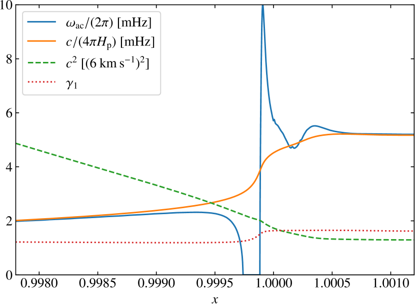
Figure 1: Acoustic cut-off frequency $\omega_{\text{ac}}$ associated with the Lagrangian pressure-perturbation eigenfunction, defined by equation (2), in the surface layers of solar model S of Christensen-Dalsgaard et al. (1996), plotted as a continuous blue curve against fractional radius $x=r/\mbox{R}_{\text{ph}}$, where $\mbox{R}_{\text{ph}}$ stands for the photospheric radius. Between about $x=0.99974$ and $x=0.99988$, $\omega_{\text{ac}}$ is imaginary, and formally wave propagation can occur at all frequencies. The continuous orange curve is the corresponding cut-off frequency adjusted according to the procedure proposed by Langer (1937) to prevent the error in the JWKB approximation to the wave equation (which experiences an appropriately smoothed background state) from approaching divergence at the phantom singular point at which pressure would vanish, leading to $\omega_{\text{ac}}\simeq c/(2H_{\text{p}})$, where $H_{\text{p}}$ is the pressure scale height. The dashed green curve is the squared adiabatic sound-speed (in units of $(6~{}\text{km}~{}\text{s}^{-1})^{2}$) and the dotted red curve is $\gamma_{1}$. The almost linear section of the squared sound-speed below $x\approx 1.0000$ could in principle be extrapolated to zero to locate a phantom singularity, as indicated by Balmforth & Gough (1990); however the deviation from linearity renders the outcome insufficiently precise for our purposes here. The top of the superadiabatically stratified convection zone is located at $r/\mbox{R}_{\text{ph}}\approx 0.99994$.

3 The principles of the structure inversion, and the radius difference

3.1 Inversion formulae that take account of radius and mass differences

3.1.1 Relation between the frequency difference and the structure difference

Typically, helioseismological inversion aims at obtaining a representation of the difference in structure between the Sun (or a target theoretical model) and a reference model that is believed to be sufficiently close to the target for linearization to be valid. The small differences in the structure variables are derived from integral equations which relate the structure differences to the eigenfrequency differences. The weighting functions in the integrands that multiply the differences (either absolute or relative) in the structure variables are called data kernels; they depend on both the eigenfunctions and the equilibrium structure, and are obtained by perturbing the full integral expressions for the eigenfrequencies. In principle the integration should extend over the entire domain occupied by the star: formally that is to infinity, but in practice it is adequate to truncate the outer limit to a surface so far beyond the region of propagation of the oscillation modes that any appropriate boundary condition contributes negligibly to the integrals. However, if the target were to be another theoretical model, that model might have a genuine surface at which pressure, and probably sound speed, vanish. We shall sometimes find it convenient to speak in terms of such target models when describing the properties of the inversion procedures. Whether the target is such a finite model, or a more realistically extended model or the real Sun, the integral representations of the eigenfrequencies essentially (that is, to a fair degree of accuracy) satisfy a variational principle (Ledoux & Walraven, 1958; Chandrasekhar, 1964), and the perturbations to the eigenfunctions do not appear in the formulae for the kernels. In more realistic situations in which the boundary conditions appear to preclude a variational principle, one can construct appropriate integral expressions for the frequency differences as a perturbation in terms of the eigenfunctions of only the reference model (cf. Veronis, 1959). That suggests that the outcome of the mathematical process of inversion that does not take explicit account of a potential radius difference can provide a correct representation of the internal structure, as we discuss below. However, it does require in addition a precise definition of a seismic radius in order to establish an appropriate scaling of the reference model.

3.1.2 Optimally localized averages of the structure

In this paper, we adopt optimally localized averaging (OLA) as the means of representing the structure differences. The averaging kernels are constructed as unimodular linear combinations of the data kernels, the coefficients $a_{n,l}$ having been determined as a trade-off between the degree of localization and the resultant magnification of the errors in the frequency data $\nu_{n,l}$; the corresponding combinations of the data, $\Sigma_{n,l}a_{n,l}\delta\nu_{n,l}/\nu_{n,l}$, are, to within data errors, averages of the true differences between the structures of the target star and the reference model. Such combinations were used originally in geophysics just to assess the resolving power of Whole-Earth data (Backus & Gilbert, 1968). But here we use the averages to represent the structural differences themselves, bearing in mind that they are not pointwise values but in some sense a smoothed version of the true differences. Treating them as pointwise values, which has been tempting to some, does not normally lead to functions that satisfy the integral relations from which they were constructed, which is why they were not used by geophysicists, at least in the early days, to represent the functions themselves. Functions that do satisfy the integral relations can easily be constructed simply by insisting, subject to certain demands introduced to render the outcome determinate, that the functions have the correct averages. One way to accomplish that is simply to determine the smoothest function that satisfies the averaging constraints. This is a typical problem in calculus of variations with constraints, which can be solved by any standard method. At this stage of our discussion, for the purposes of appreciating the outcome of the inversion it is not necessary to know how the averaging coefficients $a_{n,l}$ are determined. All that is needed, aside from the averages themselves, is to know the kernels over which the structure variables are averaged, and, of course, the uncertainties in those averages resulting directly from the uncertainties in the measured oscillation frequencies.

3.1.3 Formulae for the frequency difference taking account of radius and mass differences

As we mentioned in Section 1, in conventional helioseismological inversions it is assumed that there is no difference between the total radii $R$ of the reference model and of the Sun, nor any error in the gravitational constant $G$. In a similar fashion we obtain for the frequency differences between the Sun and the reference model, which constitute the data to be inverted:

$$\frac{\delta\nu_{n,l}}{\nu_{n,l}}=\int K_{\psi,\rho}^{(n,l)}\frac{\delta_{x}\psi}{\psi}\;\text{d}x+\int K_{\rho,\psi}^{(n,l)}\frac{\delta_{x}(G\rho)}{G\rho}\;\text{d}x+S_{n,l}\;,$$ (3)

for each mode. The details of the derivation of this equation are given in appendix A. The meanings of the symbols in equation (3) are as followings: $\nu_{n,l}$ is the cyclic frequency of the mode of radial order $n$ and spherical degree $l$ – we concentrate on the spherically averaged structure, and therefore interpret $\nu_{n,l}$ as the uniformly weighted average over azimuthal order $m$ of the singlet frequencies $\nu_{n,l,m}$ (e.g. Ritzwoller & Lavely, 1991) – $\psi$ is defined by

$$\psi:=\frac{c}{r}\;{;}$$ (4)

$\rho$ is density; $x$ is the fractional radius $r/R$, where $R$ is a fiducial (acoustic) radius of the Sun whose meaning we discuss later; $\delta_{x}f$ means the difference between some structural variable $f$ pertaining to the Sun and to the reference model at the same fractional radius $x$; and $K_{\psi,\rho}^{(n,l)}$ and $K_{\rho,\psi}^{(n,l)}$ are data kernels (Fréchet derivatives) for $\delta_{x}\psi/\psi$ and $\delta_{x}(G\rho)/(G\rho)$ respectively; $S_{n,l}$ is called a surface term, and is introduced to take account of uncertainties in the near-surface regions of the Sun (cf. Dziembowski, Pamyatnykh & Sienkiewicz, 1990). We adopt the notation in this paper that, when no explicit bounds are indicated the domain of integration ranges over the entire mass of the structure.

We point out the following important features of equation (3):

1. the expressions for the kernels $K_{\psi,\rho}^{(n,l)}$ and $K_{\rho,\psi}^{(n,l)}$ are essentially the same as those in the conventional structure inversions, which are derived under the assumption that there is no difference in the global quantities $R$ and $G$ (e.g. Gough & Thompson, 1991) ;

2. the differences $\delta_{x}\psi/\psi$ and $\delta_{x}(G\rho)/(G\rho)$ between the Sun and the reference model are taken not at the fixed radius $r$ but at the fixed fractional radius $x$, and are regarded as functions of $x$;

3. the difference in the fiducial radius $R$ is present implicitly in the expressions through the difference operator $\delta_{x}$ at fixed $x$, although here we give no physical meaning to $R$ – at this stage it is just a scale factor – we attempt to provide a physical interpretation later;

4. density $\rho$ is multiplied by the gravitational constant $G$ wherever it appears;

5. for this particular choice of structure variables, namely $\psi$ and $G\rho$, neither the difference in the total mass $M$ nor that in $GM$ appears explicitly in the expression; this is not the case for all choices of structure variables, although the current choice is not unique in this respect (see Appendix C); we emphasize that the total mass constraint (5) was not incorporated explicitly into the derivation of these data kernels. Therefore equation (3) is applicable to asteroseismology too. Gough & Kosovichev (1993) have demonstrated its use in that situation, where additional, non-seismic, data to estimate the radius and mass of the star are required.

3.1.4 Total mass constraint

The total mass constraint,

$$M=\int 4\pi r^{2}\rho\;\text{d}r\;,$$ (5)

which we usually adopt to ensure that the inversions are consistent with the observed value of the solar mass, can similarly be extended to include the difference in the total radius $R$ and the product of the gravitational constant and the total mass; it may be written:

$$\frac{\delta R}{R}=\frac{\delta(GM)}{3GM}-\int\frac{4\pi R^{3}x^{2}\rho}{3M}\frac{\delta_{x}(G\rho)}{G\rho}\;\text{d}x\;,$$ (6)

in which $\delta R$ and $\delta(GM)$ appear explicitly. Since the form of equation (6) is similar to that of equation (3), it is common practice to treat all of these equations in like manner, with no caution as to the different structural connotation. On the other hand, in the present analysis, we explicitly distinguish equation (6) from equation (3) based on their physical meanings. This is essential to discuss the radius difference between the target structure and the reference model.

3.2 Annihilator relation associated with a uniform scaling

So far we have offered no insight into the physical meaning of $R$ in equations (3) and (6). To assist thinking, we first draw attention to the following annihilator relation:

$$\int K_{\psi,\rho}^{(n,l)}\frac{{\text{d}}\ln\psi}{{\text{d}}\ln r}\;\text{d}x+\int K_{\rho,\psi}^{(n,l)}\frac{{\text{d}}\ln\rho}{{\text{d}}\ln r}\;\text{d}x=0\;,$$ (7)

for any $n$ and $l$. Appendix B provides a proof of this relation, which is closely associated with the homology relation that preserves adiabatic eigenfrequencies: if the radial coordinate is uniformly stretched by a constant factor $\lambda$ according to

$$r \rightarrow\lambda r\;,$$ (8)

and the profiles of the other seismologically accessible variables are scaled as

$$\psi(r) \rightarrow\psi(\lambda r)$$ (9)

$$G\rho(r) \rightarrow G\rho(\lambda r)\;,$$ (10)

$$R \rightarrow\lambda R$$ (11)

$$GM \rightarrow\lambda^{3}GM\;,$$ (12)

the eigenfrequencies $\nu_{n,l}$ are unchanged. There is an implicit assumption in this argument that $K_{\rho,\psi}^{(n,l)}=0$ at the upper boundary of the integral in equation (7). This homology relation can be regarded as a generalization of the popular statement in the theory of stellar pulsation that the eigenfrequency of the radial fundamental pulsation mode of a star is proportional to $\sqrt{GM/R^{3}}$. We should stress that this statement is only approximately true, whereas the homology relation is exact for all linearized adiabatic oscillations.

The homology relation demonstrates the important fact that there exists a series of (isospectral) structures that cannot be distinguished by their eigenfrequencies alone. Owing to this characteristic, it is evident that there is an ambiguity of the stretching of the radial coordinate in any outcome of inversions that disregard the total mass constraint. The isospectral structures resulting from only such stretching have different masses, so one can isolate an acceptable one according to its total mass. However, there remains a formally infinite set of seismologically acceptable structures, not necessarily with the same radius, whose differences lie in the annihilator of the data kernels.

In practice, however, one obtains results from OLA with hardly an apparent ambiguity, whether the mass constraint is included or not. Therefore any stretching factor appears to be determined implicitly in the inversion procedure. We need to know which specific value is chosen. For example, were it the case that the target structure and the reference model were actually related strictly homologously in the sense specified by equations (8)–(12), then $\delta\nu_{n,l}=0$ for all modes, and any linearized inversion in which the inferences are expressed by a linear combination of the frequency differences would result in there being no difference between (at least the localized averages of) the target and the reference. This means that the homology factor $\lambda$ in equations (8)–(12) is implicitly detected and is properly related to the scale-factor difference $\delta R$ in the inversion procedure, with $\delta_{x}\psi=0,\delta_{x}(G\rho)=0$ in equation (3). However, we do not know the value of $\delta R$ at this stage. This example suggests that there is some principle that determines the scale factor $R$ even if the differences are not homologous.

Here we make a remark about the conventional method of structure inversion, which usually assumes no difference between the radii of the target structure and the reference model. We can validly reinterpret conventional inversions if they are performed without explicit use of the total mass constraint. In that case, we should replace the labels, setting $\delta_{r}c/c$ and $\delta_{r}\rho/\rho$ to $\delta_{x}\psi/\psi$ and $\delta_{x}(G\rho)/(G\rho)$, respectively. Then we do not know the radius difference, which is required for the operator $\delta_{x}$ to be well defined, until we carry out separately the additional inversion for $\delta R$ using the total mass constraint.

In summary, we have two questions to answer here:

1. How can we know the stretching factor, $\lambda=1+\delta R/R$, that is implicitly determined in the procedure of the OLA method?

2. What kind of principle is operative in the process of determining an appropriate value of that stretching factor?

We answer question 1 immediately in the following section; question 2 is addressed in Section 4.2.

3.3 How to determine the radius difference

The total mass constraint (6), which is a physically different condition from the frequency equation (3), immediately gives us an answer to the first question. Once we have the density profile $\delta_{x}(G\rho)/(G\rho)$ without knowing what $R$, hence $x$, is, we can substitute this profile into equation (6) to get $\delta R/R$. We could also perform a different inversion for $\delta R/R$ based on equations (3) and (6), which will be described in detail in Section 4. From a physical point of view, we determine the size of the target star, which is otherwise ambiguous owing to the undetermined stretching of the radial coordinate, by constraining its total mass (actually $GM$). This answers question 1. We need to know more about the mathematics behind the OLA method for the structure, which we discuss in Section 4, before we can answer question 2.

3.4 OLA and an annihilator vector

In the OLA method we make inferences about structure variables such as sound-speed differences in the vicinity of some chosen point $x=x_{\text{t}}$ by constructing new kernels $\mathcal{K}^{(\psi)}_{\psi,\rho}$ and $\mathcal{K}^{(\psi)}_{\rho,\psi}$ as linear combinations of $K_{\psi,\rho}^{(n,l)}$ and $K_{\rho,\psi}^{(n,l)}$:

$$\begin{pmatrix}\mathcal{K}^{(\psi)}_{\psi,\rho}\\ \mathcal{K}^{(\psi)}_{\rho,\psi}\end{pmatrix}:=\sum_{n,l}a_{n,l}\begin{pmatrix}K_{\psi,\rho}^{(n,l)}\\ K_{\rho,\psi}^{(n,l)}\end{pmatrix}\,,$$ (13)

and define a localized average of $\delta_{x}\psi/\psi$ as

$$\left[\overline{\frac{\delta_{x_{\text{t}}}\psi}{\psi}}\right]_{\text{OLA}} :=\int\mathcal{K}^{(\psi)}_{\psi,\rho}(x;{x_{\text{t}}})\frac{\delta_{x}\psi}{\psi}(x)\;\text{d}x$$

$$\phantom{=}\mbox{}+\int\mathcal{K}^{(\psi)}_{\rho,\psi}(x)\frac{\delta_{x}(G\rho)}{G\rho}(x)\;\text{d}x\;,$$ (14)

by trying to demand that the averaging kernel $\mathcal{K}^{(\psi)}_{\psi,\rho}(x;x_{\text{t}})$ be localized around $x=x_{\text{t}}$ and unimodular (i.e. whose integral is unity), and that the cross-talk kernel $\mathcal{K}^{(\psi)}_{\rho,\psi}(x)$ is negligibly small everywhere. The constants $a_{n,l}$ are called inversion coefficients (and are distinct from the components of the annihilator vector $\bf a$ introduced in equation (17) below). Then $\sum_{n,l}a_{n,l}\delta\nu_{n,l}/\nu_{n,l}$ estimates the localized average of $\delta_{x}\psi/\psi$, somewhat, yet, we hope, not unduly contaminated by $\delta_{x}(G\rho)/(G\rho)$. As we have pointed out already, there is no need to enquire how the inversion coefficients $a_{n,l}$ are determined (although we do sketch a commonly adopted procedure in Section 5); to appreciate the meaning of the inversion all that is necessary is to know the averaging kernel at each target location $x_{\text{t}}$ and the corresponding cross-talk kernel. Similarly, one can attempt to construct a corresponding localized average of $\delta_{x}(G\rho)/(G\rho)$ with a localized unimodular kernel $\mathcal{K}^{(\rho)}_{\rho,\psi}$ and negligible cross-talk kernel $\mathcal{K}^{(\rho)}_{\psi,\rho}$ given by

$$\begin{pmatrix}\mathcal{K}^{(\rho)}_{\psi,\rho}\\ \mathcal{K}^{(\rho)}_{\rho,\psi}\end{pmatrix}:=\sum_{n,l}b_{n,l}\begin{pmatrix}K_{\psi,\rho}^{(n,l)}\\ K_{\rho,\psi}^{(n,l)}\end{pmatrix}\;.$$ (15)

Were the averages to be well localized everywhere, one could attempt to construct plausible pointwise representations of $\delta_{x}\psi/\psi$ and $\delta_{x}(G\rho)/(G\rho)$ to estimate the cross-talk integrals, and so iterate on the procedure for determining the optimally averaged differences given by equation (14) and the corresponding equation for $\overline{\delta_{x}(G\rho)/(G\rho})$. In practice that is not entirely straightforward for achieving the precision required in this endeavour.

We refer to the space spanned by the kernels $(K_{\psi,\rho}^{(n,l)},K_{\rho,\psi}^{(n,l)})$ as the kernel space; its orthogonal complement is called the annihilator. Because relation (7) can be interpreted as the vanishing of the inner product of the kernel vectors

$$\begin{pmatrix}K_{\psi,\rho}^{(n,l)}\\ K_{\rho,\psi}^{(n,l)}\end{pmatrix}$$ (16)

and the annihilator vector

$$\mathbf{a}:=\begin{pmatrix}\displaystyle\frac{{\text{d}}\ln\psi}{{\text{d}}\ln r}\\[8.53581pt] \displaystyle\frac{{\text{d}}\ln\rho}{{\text{d}}\ln r}\end{pmatrix}\;$$ (17)

for all modes, we can say that the kernel vectors given by equations (13) and (15) are orthogonal to the annihilator vector $\mathbf{a}$. In fact, we easily find from equation (7) that

$$\int\mathcal{K}^{(\psi)}_{\psi,\rho}\,\frac{{\text{d}}\ln\psi}{{\text{d}}\ln r}\;\text{d}x+\int\mathcal{K}^{(\psi)}_{\rho,\psi}\,\frac{{\text{d}}\ln\rho}{{\text{d}}\ln r}\;\text{d}x$$

$$=\sum_{n,l}a_{n,l}\left(\int K_{\psi,\rho}^{(n,l)}\,\frac{{\text{d}}\ln\psi}{{\text{d}}\ln r}\;\text{d}x+\int K_{\rho,\psi}^{(n,l)}\,\frac{{\text{d}}\ln\rho}{{\text{d}}\ln r}\;\text{d}x\right)$$

$$=0\;.$$ (18)

This means that inferences from OLA such as that given by equation (14), without the total mass constraint (6), are never influenced by the annihilator vector (17) of the target quantities $\delta_{x}\psi/\psi$ and $\delta_{x}(G\rho)/(G\rho)$. We note that at least one component of the annihilator vector (17) is quite large, or even divergent, at the stellar surface where pressure, density and temperature are all very small. This is characterized by the fact that the norm

$$I_{\text{A}}(x_{0}):=\int_{0}^{x_{0}}\left\{\left(\frac{{\text{d}}\ln\psi}{{\text{d}}\ln r}\right)^{2}+\left(\frac{{\text{d}}\ln\rho}{{\text{d}}\ln r}\right)^{2}\right\}\;\text{d}x\;,$$ (19)

can be extremely large, or even divergent, as $x_{0}$ approaches its ‘surface’ value, which we denote by $x_{{\text{surf}}}$. We are mindful to define $x_{{\text{surf}}}$ formally as the vanishing point of the density distribution, recognizing that its value might be infinite if there were no distinct surface. If that be so, then $I_{\text{A}}(x_{{\text{surf}}})$ would also be formally infinite; however, its role in determining $\delta R/R$, as in equation (39) below, is via a non-divergent limiting process of the ratio of two individually divergent integrals.

We note that there must exist annihilator vectors other than the one given by equation (17) that satisfy orthogonality relations similar to equation (7). For example, if the kernels of the eigenmodes included in the structure inversion are all negligibly small in some region, which typically happens outside of the propagation cavities, the structure in those regions cannot be probed by the eigenmodes. Therefore in practice the structure difference in such regions should be attributed to the annihilator. There are also annihilator vectors that are large within the propagation cavities, but if a wide variety of modes are included in the inversions, they are likely to be highly oscillatory (e.g. Wiggins, 1972; Gough, 1985).

Finally, we emphasize that, as evinced by equation (3), any component of the actual structure-difference vector $(\delta_{x}\psi/\psi,\delta_{x}(G\rho)/G\rho)$ that is orthogonal to all the kernel vectors $(K_{\psi,\rho}^{(n,l)},K_{\rho,\psi}^{(n,l)})$ makes no contribution to the frequency data $\delta\nu_{n,l}/\nu_{n,l}$, and so cannot be inferred seismologically. Therefore the seismologically accessible element of the structure-difference vector must lie in the kernel space, and can be represented as a linear combination of the kernel vectors, as in equation (32). This forms the basis of some regularized least-squares data-fitting inversion procedures. It is also explicit in OLA (equation(14)). In fact, since the localized averages are totally insensitive to the annihilator vectors included in the structure-difference vector, the averages can be interpreted as those of only the element of the difference vector in the kernel space.

4 Seismic radius inversion based on p-mode frequencies

4.1 An inversion for the scale factor

We first describe a method, based on a procedure analogous to the OLA inversion for the structure variables, to infer the radius difference defining the scale factor $1+\delta R/R$.

By making a linear combination of equations (3) and (6) with coefficients $c_{n,l}$, we obtain

$$\frac{\delta R}{R}=\sum_{n,l}c_{n,l}\frac{\delta\nu_{n,l}}{\nu_{n,l}}-\mathcal{C}-\mathcal{S}+\frac{1}{3}\frac{\delta(GM)}{GM}\;,$$ (20)

in which

$$\mathcal{C}:=\int\mathcal{K}^{(R)}_{\psi,\rho}\frac{\delta_{x}\psi}{\psi}\;\text{d}x+\int\mathcal{K}^{(R)}_{\rho,\psi}\frac{\delta_{x}(G\rho)}{G\rho}\;\text{d}x\;,$$ (21)

and $\mathcal{S}$ is the contribution from the surface terms, given by

$$\mathcal{S}:=\sum_{n,l}c_{n,l}S_{n,l}\;.$$ (22)

The symbols $\mathcal{K}^{(R)}_{\psi,\rho}$ and $\mathcal{K}^{(R)}_{\rho,\psi}$ in equation (21) are defined by

$$\mathcal{K}^{(R)}_{\psi,\rho} {:=}\sum_{n,l}c_{n,l}K_{\psi,\rho}^{(n,l)}$$ (23)

$$\mathcal{K}^{(R)}_{\rho,\psi} {:=}\sum_{n,l}c_{n,l}K_{\rho,\psi}^{(n,l)}+\frac{4\pi R^{3}x^{2}\rho}{3M}\;,$$ (24)

respectively. Note that the total-mass constraint is included here. This formulation is formally similar to the one for the mean-density inversion by Reese et al. (2012) in asteroseismology. The differences are that the value of $GM$ is accurately known for the Sun, and that we adopt $\psi$ and $G\rho$ as the target structure variables, while Reese et al. adopt $\rho$ and $\gamma_{1}$.

The coefficients $c_{n,l}$ are determined as a trade-off between minimizing the magnitude of $\mathcal{C}$ and limiting the magnification of the frequency errors, simultaneously preventing $\mathcal{S}$ from influencing the inferences. This is accomplished by minimizing with respect to $c_{n,l}$ the quantity

$$\chi^{2}_{R}:=\alpha_{R}\int({\mathcal{K}^{(R)}_{\psi,\rho}})^{2}\;\text{d}x+\beta_{R}\int({\mathcal{K}^{(R)}_{\rho,\psi}})^{2}\;\text{d}x+\gamma_{R}{\sigma}^{2}\;$$ (25)

under the condition that a representation of $\mathcal{S}$, which is defined below, vanishes; $\sigma$ is a formal error (also defined below, by equation (27)), and $\alpha_{R}$, $\beta_{R}$ and $\gamma_{R}$ are adjustable parameters. An estimate of $\delta R/R$ is then given by

$$\left(\frac{\delta R}{R}\right)_{\text{ac}}{:=}\sum_{n,l}c_{n,l}\frac{\delta\nu_{n,l}}{\nu_{n,l}}\pm\sigma\;,$$ (26)

where we have assumed that $\delta(GM)/(GM)=0$: we are constructing a representation of the Sun with precisely the same value of $GM$ as that of our reference model, although we appreciate that that value may be in error by an amount of order $\sigma_{GM}$. The formal error $\sigma$ is given by

$$\sigma^{2}:=\sum_{n,l}\left(c_{n,l}\sigma_{n,l}\right)^{2}+\left(\frac{\sigma_{GM}}{3}\right)^{2}\;,$$ (27)

in which $\sigma_{GM}$ and $\sigma_{n,l}$ denote the relative observational standard errors in the product $G\mbox{M}_{\sun}$ (cf. Table 1) and the frequencies $\nu_{n,l}$, respectively. We recall that $(\delta R/R)_{\text{ac}}$ defines a scaling based on the acoustic structure of the star, and accordingly we have adopted the subscript ‘ac’.

In carrying out the radius inversions we take special care with the surface term by taking account of its leading $l$ dependence (Gough & Vorontsov, 1995; Di Mauro et al., 2002). The explicit expression we adopt is

$$S_{n,l}=\frac{1}{I_{n,l}}\left\{F_{0}(\nu_{n,l})+\left(\frac{l+1/2}{\nu_{n,l}}\right)^{2}F_{2}(\nu_{n,l})\right\}\;,$$ (28)

where $I_{n,l}$ is the mode inertia normalized by that of the radial mode with almost the same frequency (cf. Christensen-Dalsgaard & Berthomieu, 1991), and the functions $F_{0}$ and $F_{2}$ are arbitrary, and depend only on frequency. Both $F_{0}$ and $F_{2}$ are expanded as series of $n_{0}$ and $n_{2}$ Legendre polynomials, respectively, whose arguments are normalized so that the whole range of the frequencies that are included in the representation corresponds to the interval $[-1,1]$. To ensure that $\mathcal{S}$ vanishes, we adopt Lagrange’s method of undetermined multipliers to obtain the coefficients in the Legendre expansions during the minimization of $\chi^{2}_{R}$. The resulting values of $(\delta R/R)_{\text{ac}}$, for several values of $n_{0}$ and $n_{2}$ , are listed below in Table 4.

Although our formulation does not explicitly distinguish p modes from f modes (nor, even, g modes), in practice it is not a good idea to mix both types of modes in the structure and radius inversion, because the functional form of the surface term for p modes is likely to be qualitatively different from that for f modes, owing to their different responses to near-surface perturbations (cf. Gough, 1993; Di Mauro et al., 2002), as we point out in Section 7.

4.2 Interpretation of the inverted $\delta R/R$

Although a formal procedure to obtain $(\delta R/R)_{\text{ac}}$ given by equation (26) has been developed in Section 4.1, we still need to consider how to interpret the result. To this end we examine the requirement of the inversion procedure in Section 4.1 that the contribution from $\mathcal{C}$ to $\delta R/R$ be rendered negligible (cf. equation (20)). The outline of the discussion is as follows: though it might appear at first sight that this requirement can be satisfied easily if the frequencies of a sufficient number of eigenmodes with different characters are available, it is actually impossible to satisfy it if the annihilator vector $\mathbf{a}$ seriously ‘contaminates’ the relative structure difference, $\left(\delta_{x}\psi/\psi,\,\delta_{x}\left(G\rho\right)/\left(G\rho\right)\right)$; this contamination can be removed only if the definition of $x$, or equivalently $\delta R/R$, is adjusted appropriately, and we claim that only in this case does the inversion procedure provide a meaningful answer; we interpret the outcome of the inversion given by equation (26) as that value of $\delta R/R$ that makes the relative structure difference almost free from the annihilator vector $\mathbf{a}$, as we now discuss.

Perusal of equation (20) for $\delta R/R$ reveals that the right-hand side itself depends on $\delta R$, via the difference operator $\delta_{x}$ that appears in $\mathcal{C}$. The transformation between $\delta_{x}$ and $\delta_{r}$ is given explicitly by

$$\begin{pmatrix}\displaystyle\frac{\delta_{r}c}{c}\\[8.53581pt] \displaystyle\frac{\delta_{r}(G\rho)}{G\rho}\end{pmatrix}=\begin{pmatrix}\displaystyle\frac{\delta_{r}\psi}{\psi}\\[8.53581pt] \displaystyle\frac{\delta_{r}(G\rho)}{G\rho}\end{pmatrix}=\begin{pmatrix}\displaystyle\frac{\delta_{x}\psi}{\psi}\\[8.53581pt] \displaystyle\frac{\delta_{x}(G\rho)}{G\rho}\end{pmatrix}-\frac{\delta R}{R}\mathbf{a}.$$ (29)

It is important to realize that the decomposition on the right-hand side of equation (29) is in a sense arbitrary, as we discussed in the introduction. To render it determinate requires another constraint, which we are free to choose at will. We pay attention to the main assumption upon which equation (26) relies: that with enough modes of sufficiently diverse variety the contribution from $\mathcal{C}$ can be made negligible; the coefficients $c_{n,l}$ have been determined in such a way as to make $\mathcal{S}$ vanish, and the uncertainty in $GM$ is much smaller than that of the other quantities influencing our analysis, so that, aside from frequency-measurement errors, the term $\mathcal{C}$ contaminating the approximation (26) to equation (20) is all that remains to degrade the estimate. An essential point is that, because the magnitude of the annihilator vector $\mathbf{a}$ given by equation (17) is large near the stellar surface, if it is included in the fractional structure difference at fixed $x$, expressed by the second term on the right-hand side of equation (29), its contribution to $\mathcal{C}$ is not negligible, however small we can make $\mathcal{K}^{(R)}_{\psi,\rho}$ and $\mathcal{K}^{(R)}_{\rho,\psi}$ by adjusting the coefficients $c_{n,l}$. This can be understood explicitly from the following expression for the projection of the annihilating vector function $\mathbf{a}$ onto the kernels of $\mathcal{C}$:

$$\int\mathcal{K}^{(R)}_{\psi,\rho}\frac{{\text{d}}\ln\psi}{{\text{d}}\ln r}\;\text{d}x+\int\mathcal{K}^{(R)}_{\rho,\psi}\frac{\text{d}\ln\rho}{\text{d}\ln r}\;\text{d}x$$

$$=\int\frac{4\pi R^{3}x^{2}\rho}{3M}\frac{\text{d}\ln\rho}{\text{d}\ln r}\;\text{d}x=-1\;,$$ (30)

which can be derived from equations (23), (24), (7), and (5), assuming that density vanishes, or is at least negligible, at the surface. Evidently, that projection is not small. In other words, the assumption of negligible contribution from $\mathcal{C}$ cannot be justified without adjusting the decomposition given by equation (29).

To obtain an appropriate adjustment we explicitly distinguish the seismologically accessible element from the annihilator vector thus:

$$\begin{pmatrix}\displaystyle\frac{\delta_{r}\psi}{\psi}\\[8.53581pt] \displaystyle\frac{\delta_{r}\left(G\rho\right)}{G\rho}\end{pmatrix}=\begin{pmatrix}\displaystyle\frac{\delta_{r}\psi}{\psi}\\[8.53581pt] \displaystyle\frac{\delta_{r}\left(G\rho\right)}{G\rho}\end{pmatrix}_{\text{ker}}+\begin{pmatrix}\displaystyle\frac{\delta_{r}\psi}{\psi}\\[8.53581pt] \displaystyle\frac{\delta_{r}\left(G\rho\right)}{G\rho}\end{pmatrix}_{\text{a}}\;,$$ (31)

where

$$\begin{pmatrix}\displaystyle\frac{\delta_{r}\psi}{\psi}\\[8.53581pt] \displaystyle\frac{\delta_{r}\left(G\rho\right)}{G\rho}\end{pmatrix}_{\text{ker}}:=\sum_{n,l}k_{n,l}\begin{pmatrix}K_{\psi,\rho}^{\left(n,l\right)}\\ K_{\rho,\psi}^{\left(n,l\right)}\end{pmatrix}$$ (32)

is the seismologically estimated accessible element of the actual structure difference $\left(\delta_{r}\psi/\psi,\,\delta_{r}\left(G\rho\right)/\left(G\rho\right)\right)$ that lies in the kernel space, from which we wish to achieve a reliable estimate of $\mathcal{C}$. Equation (32) is sometimes called a spectral expansion (e.g. Section 41.1.1 of Unno et al., 1989). Note that the second term on the right-hand side of equation (31) can generally include not only a term proportional to $\mathbf{a}$, but also other vectors in the annihilator. We note also that $({\delta_{r}\psi}/{\psi},{\delta_{r}\left(G\rho\right)}/{G\rho})_{\text{ker}}$ corresponds to the projection of the structure difference onto the kernel space. The reason why it is seismologically accessible is that the right-hand side of equation (3), without the surface term $S_{n,l}$, can be interpreted as a nontrivial inner product of the structure difference with the kernel vectors. On substituting equations (29) and (31) into equation (21), we obtain with the help of equation (30)

$$\mathcal{C}=\mathcal{C}_{\text{ker}}-\frac{\delta R}{R}+\int\frac{4\pi R^{3}x^{2}\rho}{3M}\left(\frac{\delta_{r}\left(G\rho\right)}{G\rho}\right)_{\text{a}}\;\text{d}x\;,$$ (33)

in which

$$\mathcal{C}_{\text{ker}}:=\int\mathcal{K}_{\psi,\rho}^{(R)}\left(\frac{\delta_{r}\psi}{\psi}\right)_{\text{ker}}\;\text{d}x+\int\mathcal{K}_{\rho,\psi}^{(R)}\left(\frac{\delta_{r}\left(G\rho\right)}{G\rho}\right)_{\text{ker}}\;\text{d}x\;.$$ (34)

Since $\mathcal{C}_{\text{ker}}$ depends on only the seismologically accessible element, we may adopt as the fundamental assumption of the inversion procedure in Section 4.1 that $\mathcal{C}_{\text{ker}}$ can be made negligibly small by adjusting the coefficients $c_{n,l}$ appropriately if we have a sufficient number of eigenmode kernels with different characters. Since the estimate for $\delta R/R$ given by equation (26) is meaningful only when $\mathcal{C}$ is negligible as a whole, we interpret, based on equation (33), that it is the estimate in the case where $\delta R/R$ is set to

$$\left(\frac{\delta R}{R}\right)_{\text{interpret}}=\int\frac{4\pi R^{3}x^{2}\rho}{3M}\left(\frac{\delta_{r}\left(G\rho\right)}{G\rho}\right)_{\text{a}}\;\text{d}x\;.$$ (35)

Seemingly paradoxically at first, equation (35) appears to imply that the relative difference in the scale factor is determined by the element of the density-profile difference that is not accessible to the eigenfrequencies. Of course, that is fully consistent with the isospectral nature of the problem that is discussed in Sections 3.2 and 3.3.

Finally, we note that the minimization of the influence of the contaminating integral $\mathcal{C}$ in expression (20) for $\delta R/R$ answers question 2 at the end of Section 3.2.

4.3 Mode-set independent interpretation

Because the annihilator necessarily depends on the mode set available, so does the interpretation given by equation (35). To obtain an expression for $\delta R/R$ that is only weakly dependent of the mode set, we consider there to be such a large variety of modes available that the annihilator space can be assumed to be composed of only the vector $\mathbf{a}$ defined by equation (17) – together, of course, with the highly oscillatory functions which we accept cannot be resolved, and which accordingly we ignore. This assumption permits replacing equation (31) by

$$\begin{pmatrix}\displaystyle\frac{\delta_{r}c}{c}\\[8.53581pt] \displaystyle\frac{\delta_{r}(G\rho)}{G\rho}\end{pmatrix}=\begin{pmatrix}\displaystyle\frac{\delta_{r}c}{c}\\[8.53581pt] \displaystyle\frac{\delta_{r}(G\rho)}{G\rho}\end{pmatrix}_{\text{ker}}-\frac{\delta R}{R}\mathbf{a}$$ (36)

(cf. equation (29)). Recognizing that both components of $\mathbf{a}$ are typically quite large near the surface, and that the frequency kernels, which are the constituents of the spectral expansion, are very small, we neglect the first term on the right-hand side of equation (36) and are led to the estimates

$$\left(\frac{\delta R}{R}\right)_{c}{:=}\lim_{x_{0}\rightarrow x_{{\text{surf}}}}\frac{\displaystyle\frac{\delta_{r}c}{c}(x_{0})}{\displaystyle-\frac{{\text{d}}\ln\psi}{{\text{d}}\ln r}(x_{0})}$$ (37)

and

$$\left(\frac{\delta R}{R}\right)_{\rho}{:=}\lim_{x_{0}\rightarrow x_{{\text{surf}}}}\frac{\displaystyle\frac{\delta_{r}(G\rho)}{G\rho}(x_{0})}{\displaystyle-\frac{{\text{d}}\ln\rho}{{\text{d}}\ln r}(x_{0})}\;.$$ (38)

We may expect equation (38) to converge faster than equation (37) because $\left|{\text{d}}\ln\rho/{\text{d}}\ln r\right|$ is much larger than $\left|{\text{d}}\ln\psi/{\text{d}}\ln r\right|$ in realistic stellar structures. In fact, $\left|{\text{d}}\ln\psi/{\text{d}}\ln r\right|$ can actually be quite small in the vicinity of the temperature minimum, in which case our argument formally breaks down because equation (37) is not well satisfied.

Note that by taking the inner product of equation (36) with $\mathbf{a}$, we obtain

$$\left(\frac{\delta R}{R}\right)_{\text{integral}}{:=}$$

$$\lim_{x_{0}\rightarrow x_{{\text{surf}}}}\frac{-1}{I_{\text{A}}(x_{0})}\int_{0}^{x_{0}}\left(\frac{\delta_{r}c}{c}\frac{{\text{d}}\ln\psi}{{\text{d}}\ln r}+\frac{\delta_{r}(G\rho)}{G\rho}\frac{{\text{d}}\ln\rho}{{\text{d}}\ln r}\right)\;\text{d}x\;,$$ (39)

in which $I_{\text{A}}(x_{0})$ is defined by equation (19). One might expect this expression to be more robust because it is somewhat less susceptible to the details of the relatively small-scale variation of the structure of the star near its surface (see Section 6.2). That is indeed the case, as is illustrated in Fig. 2, in which the right-hand sides of equations (38) and (39), obtained from the difference between two theoretical solar models, are plotted against $x_{0}$ in the outer layers. We have not included a corresponding estimate from equation (37), but merely report that it oscillates more wildly than the estimate from equation (38). We emphasize that the resulting total radius is, in principle, independent of the reference model from which it was obtained.

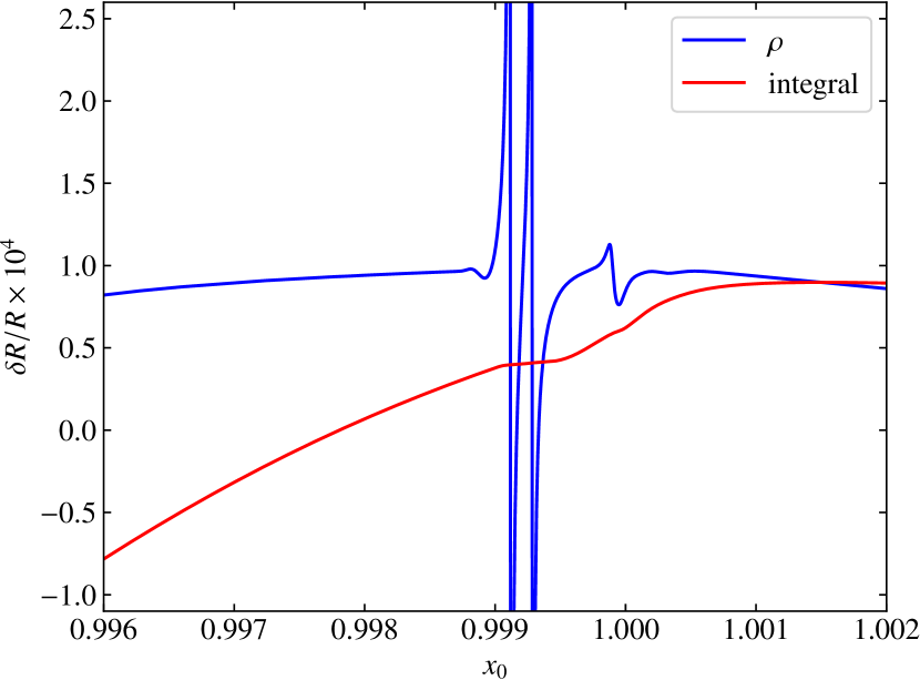
Figure 2: Estimates of $\delta R/R$ given by equation (38) (blue) and equation (39) (red) relating a target theoretical solar model to a reference model, model S of Christensen-Dalsgaard et al. (1996), plotted against the value $x_{0}$ of $r/\mbox{R}_{\text{ph}}$ in the outer layers. Here, $\mbox{R}_{\text{ph}}$ means the photospheric radius. The target model is essentially model 1 of Houdek & Gough (2007), scaled to a photospheric radius $1.0001\,\mbox{R}_{\text{ph}}$. Additional information about that model is provided in Section 6.1.

4.4 Relation to the acoustic radius

We finally consider how to interpret $\left(\delta R/R\right)_{\text{ac}}$, given by equation (26), in terms of the seismic radii, which are introduced in Section 2. As is illustrated by Takata & Gough (2003), the density profile near the surface, where the kernels start to decay outwards in response to acoustic reflection, is crucial in determining the p-scaled radius difference $\delta R/R$; that is true also for the f-scaled radius (Schou et al., 1997; Dziembowski et al., 2001). It is therefore clear that the density profile in the vicinity of the upper turning points is the most important characteristic for determining the p-scaled radius. In fact, it tells us that the difference in the p-scaled radius can be interpreted as the homologous difference in the density profile around the upper turning points. This means that, if the density $\rho$ itself becomes much smaller than the density difference $\delta_{r}\rho$ near the surface, the inversion procedure (without the total mass constraint) attributes the large relative difference $\delta_{r}\rho/\rho$ to the homologous difference so that the scaled difference $\delta_{x}(G\rho)/(G\rho)$ is prevented from being too large near the surface. It seems as if the inversion procedure adjusts the scale factor $R$ to render the assumption of the linearization to be as near to being valid as possible.

In order to understand further the relation between the density and the radius difference, we summarize the density profile near the surface of the Sun based on model S. The atmosphere around the temperature minimum, which is located $\sim 500~{}\text{km}$ above the photosphere, can be well approximated by an isothermal structure, which implies the density decreases exponentially outwards with a constant scale height. The scale height gradually gets larger with diminishing height above the photosphere, where it is approximately equal to ${180}~{}\text{km}$ (${2.6}\times 10^{-4}$ in fractional radius). Beneath the photosphere, it first increases very rapidly until it reaches its local maximum at a depth of $\sim 80~{}\text{km}$ below the photosphere, and then decreases steeply until it takes its local minimum at a depth of $\sim{250}~{}\text{km}$, after which it turns to increase inwards mildly. Note that the seismic radius $\mbox{R}_{{\text{ac}}}$, which was described in Section 2, is located very close to the local maximum of the density scale height. Because physical processes in the atmosphere can be understood relatively well, we may assume that the density-profile difference between the Sun and the reference model is small between the photosphere and the temperature minimum, except for a possible displacement due to the position difference in the photosphere. Since $\mbox{R}_{\text{ph}}$ is quite close to $\mbox{R}_{{\text{ac}}}$, the difference in the atmosphere can largely be removed by stretching (or contracting) the radial coordinate of the reference model to make $\mbox{R}_{{\text{ac}}}$ consistent with the Sun. This essentially corresponds to eliminating the annihilator component, which is represented by the second term on the right-hand side of equation (36), from the density difference. We thus identify

$$\left(\frac{\delta R}{R}\right)_{\text{ac}}=\frac{\delta\mbox{R}_{{\text{ac}}}}{\mbox{R}_{{\text{ac,r}}}}$$ (40)

(cf. equation (1)). Note that there could remain a small difference in the density structure above $\mbox{R}_{{\text{ac}}}$, even after the adjustment. This may originate from uncertainties in the description of the superadiabatic convective layers, which contain $\mbox{R}_{{\text{ac}}}$.

5 Structure Inversions with radius difference

Because in conventional structure inversions the difference between the photospheric radius of the Sun and that of the reference model is usually ignored (see Richard et al., 1998), it behoves us now to offer a modification. We concentrate particularly on inversions for sound speed and density. We expand, in Sections 5.1 and 5.2, a method to obtain inferences about $\delta_{x}c/c$ and $\delta_{x}(G\rho)/(G\rho)$ which depend on $\delta R/R$ only implicitly through the definition of $x=r/R$; then we can determine the radius difference $\delta R/R$ independently by the method described in Section 4.

5.1 Formulation of the sound-speed inversion

The basic equation of the analysis can be obtained as a linear combination of equations (3) and (6), using equations (4) and (71), yielding

$$\sum_{n,l}e_{n,l}\frac{\delta\nu_{n,l}}{\nu_{n,l}} =\int\mathcal{K}^{(c)}_{c,\rho}\frac{\delta_{x}c}{c}\;\text{d}x+\int\mathcal{K}^{(c)}_{\rho,c}\frac{\delta_{x}(G\rho)}{G\rho}\;\text{d}x$$

$$\phantom{=}\mbox{}+\left(1-\int\mathcal{K}^{(c)}_{c,\rho}\;\text{d}x\right)\frac{\delta R}{R}-\frac{1}{3}\frac{\delta(GM)}{GM}+\mathcal{S}\;,$$ (41)

in which $\mathcal{K}^{(c)}_{c,\rho}$ and $\mathcal{K}^{(c)}_{\rho,c}$ are defined by

$$\begin{pmatrix}\mathcal{K}^{(c)}_{c,\rho}\\ \mathcal{K}^{(c)}_{\rho,c}\end{pmatrix}:=\sum_{n,l}e_{n,l}\begin{pmatrix}K_{c,\rho}^{(n,l)}\\ K_{\rho,c}^{(n,l)}\end{pmatrix}+\begin{pmatrix}0\\ \frac{4\pi R^{3}x^{2}\rho}{3M}\end{pmatrix}\,.$$ (42)

Here, $e_{n,l}$ are potential inversion coefficients. Within the framework of the SOLA inversion (Pijpers & Thompson, 1992) an inference about the sound speed at the fractional radius $x_{\text{t}}$ can be made by minimizing the quantity

$$\chi^{2}_{c}{:=}\int\left[\mathcal{K}^{(c)}_{c,\rho}-T(x;x_{\text{t}})\right]^{2}\;\text{d}x+\alpha_{c}\int\left({\mathcal{K}^{(c)}_{\rho,c}}\right)^{2}\;\text{d}x+\beta_{c}\sigma^{2}$$ (43)

under the unimodular normalization condition

$$\int\mathcal{K}^{(c)}_{c,\rho}\;\text{d}x=1$$ (44)

together with the vanishing of the surface term. Here the target kernel $T(x;x_{\text{t}})$ is usually taken to be a Gaussian function centred at $x=x_{\text{t}}$ with an adjustable width chosen so as to limit undue magnification of the data errors. Positive constants $\alpha_{c}$ and $\beta_{c}$ are adjustable parameters, and the formal error $\sigma$ is still given by equation (27) (with $c_{n,l}$ replaced by $e_{n,l}$).

In deriving equation (41) we have transformed the dependent variable $\delta_{x}\psi$ in equation (3) to $\delta_{x}c$ according to $\delta_{x}\psi/\psi=\delta_{x}c/c-\delta R/R$, partly because $c$ is of greater interest to astrophysicists, and, interestingly, because the influence of $\delta R/R$ is explicitly removed from equation (41) by condition (44), which is adopted also, both here and in subsection 3.4, as a convenient normalization of the localized averaging kernel.

What we obtain by minimizing $\chi_{c}^{2}$ are the inversion coefficients $e_{n,l}$, from which the difference in the sound speed in the vicinity of $x_{\text{t}}$ is estimated by

$$\left[\overline{\frac{\delta_{x}c}{c}}\right]_{\text{OLA}}{:=}\sum_{n,l}e_{n,l}\frac{\delta\nu_{n,l}}{\nu_{n,l}}+\frac{1}{3}\,\frac{\delta(GM)}{GM}$$ (45)

with the formal error $\sigma$. The averaged sound-speed difference is to be regarded as a function of $x$. Since the product $GM$ of the Sun is measured very accurately (see Table 1), we can neglect the second term on the right-hand side of equation (45). Correspondingly, the relative error $\sigma_{GM}$ contributes little to the formal error $\sigma$ in equation (27). In fact, expressions (43) and (44) do not look new at all because both of them are also found in conventional inversions. The only difference is that the coefficient of the total mass constraint (6) is now fixed at $1/3$ in the current formulation when we make the linear combination (41), whereas it is determined by minimizing a quantity like $\chi_{c}^{2}$ in equation (43) in conventional inversions. We should stress that by repeating the argument presented in Section 4.2 it follows that the interpretation of $\delta R/R$ here is the same as that given by equation (35); and it applies also for the density inversion addressed in the next section.

5.2 Formulation of the density inversion

Unlike in the sound-speed inversion, we should not include in the density inversion the total mass constraint (6), which contains a term proportional to $\delta R/R$; we need only equation (3) to get inferences of $\delta_{x}(G\rho)/(G\rho)$ without the explicit effect of $\delta R/R$. Actually, the procedure is simply the same as the conventional one without the total mass constraint. The most important difference between the two procedures is in the interpretation of the results: namely, what is regarded as $\delta_{r}\rho/\rho$ in the conventional method should be recognized as $\delta_{x}(G\rho)/(G\rho)$ in the new method. Because the gravitational constant $G$ is always multiplied by $\rho$, or, equivalently $M$, the uncertainty in $G$ itself cannot affect the inversion process. Therefore one cannot determine by helioseismology alone whether or not $\delta G$ is zero.

6 Numerical tests

In this section, we test, based on theoretical models, the formulae for the radius difference proposed in Section 4.3, and the inversion procedures for the radius, sound speed and density that are developed in Sections 4.1, 5.1 and 5.2, respectively.

6.1 Reference and target models

We use two theoretical solar models in this section, model S of Christensen-Dalsgaard et al. (1996) and model 1 of Houdek & Gough (2007), which are adopted as reference and target models, respectively. Model 1 has an age of $4.15\,{\text{Gy}}$ and a heavy-element abundance $Z=0.0200$; no gravitational settling was incorporated in its construction. By comparison, the age of model S is $4.60\,{\text{Gy}}$, the initial heavy-element abundance is $Z_{0}=0.01963$, and it has suffered gravitational settling. The models have the same photospheric radius: $\mbox{R}_{\text{ph}}=695.99$ Mm, consistent with the value of Allen (1973) (see Table 1), and the surface luminosity ($3.846\times 10^{33}$ erg $\text{s}^{-1}$); they were constructed with different opacity tables. Both models were extended by smoothly adding isothermal atmospheres out to a radius of $1.002\,{\mbox{R}_{\text{ph}}}$. The radius variable of the target model was then multiplied by a factor 1.0001 in Section 6.2 and $0.9999$ in Sections 6.3 and 6.4, and its density and sound speed were scaled homologously.

6.2 Expressions for the radius difference

We remark here simply that evidence for the accuracy of the two explanatory formulae (38) and (39) is presented in Fig. 2. Both expressions (38) and (39) are functions that flatten with increasing height in the atmosphere; the integral expression (39) tends to a constant, although $-(\delta_{r}(G\rho)/{G\rho})/({\text{d}}\ln\rho/{\text{d}}\ln r)$ declines slowly. The relative difference between the photospheric radii of the two models is $10^{-4}$, whereas the values obtained by the two formulae are both about $0.9\times 10^{-4}$. The $10^{-5}$ discrepancy, which arises at least in part from the non-homologous difference between the two models above their turning points, provides an indication of the accuracy of these formulae.

6.3 Radius inversion

We have performed a test calculation to assess the accuracy of the radius inversion method formulated in Section 4.1. To ensure that the computed oscillation eigenfrequencies faithfully represent the equilibrium models, slight adjustments were made to those models by recomputing hydrostatic balance to high precision (to order $10^{-6})$, retaining the variation of density and buoyancy frequency as the defining properties. The relative differences in the sound speed and density between the adjusted and original models are of the order of $10^{-5}$ or less for $0.05\leq r/\mbox{R}_{\text{ph}}\leq 0.95$, where $\mbox{R}_{\text{ph}}$ means photospheric radius, while the central values of the sound speed and density are lower in the adjusted models by about $0.05$ per cent and $0.1$ per cent, respectively. In addition, these evolutionary models are artificially extended by $0.5$ per cent in radius to the higher layers in the isothermal atmosphere in order to ensure that the mode kernels have negligibly small amplitude at the outermost mesh point. The structure of model 1 was shrunk homologously in the radial direction by $0.01$ per cent, and increased in density and sound speed at each value of the mass coordinate by $0.03$ per cent and $0.005$ per cent, respectively; that implies a very slight alteration to the equation of state. Since the target model so constructed has the same mass as the original model, but a smaller photospheric radius, by $0.01$ per cent, each mode frequency is augmented by $0.015$ per cent. We point out that the structure difference between the target and reference models is not homologous.

The difference between the radii of the two models was inferred from the difference in their adiabatic eigenfrequencies, which were computed by the program described by Takata & Löffler (2004). The mode set adopted was that of the MDI 360-day data (Schou, 1999), excluding the f modes. We used in total 2008 eigenmodes with degrees ranging from $l=0$ to $189$, and having frequencies between $900$ and $4600$ mHz. The frequency error of each mode of the target model was assumed to be the same as that of the corresponding mode in the MDI data. The surface term was ignored in this test. The inferred value of ${(}\delta R/R{)_{\text{ac}}}$ is $\left(-1.2\pm 0.4\right)\times 10^{-4}$ for a set of the parameters $\left(\alpha_{R},\,\beta_{R},\,\gamma_{R}\right)=\left(1,\,300,\,2\times 10^{5}\right)$. Because the frequencies used are free from observational errors, the uncertainties in the inference (of $4\times 10^{-5}$) should be regarded as being only formal. On the other hand, the systematic error, which originates from the neglected nonlinear term of the order of $(\delta\nu_{n,l}/\nu_{n,l})^{2}$ in equation (3), could be estimated to be of the order $10^{-5}$. In order to examine the stability of the radius inversion, we change the maximum spherical degree, $l_{\max}$, of the mode set, but keep the same values of $\alpha_{R}$, $\beta_{R}$ and $\gamma_{R}$. Table 3 shows the results for $l_{\max}=120$, $140$, $160$ and $189$. Although the results decrease slightly as $l_{\max}$ increases from $l_{\max}=120$ to $l_{\max}=189$, they are all consistent with each other within $2\times 10^{-5}$. From these test inversions, we conclude that the inferred relative difference in the p-scaled radius is consistent with that in the photospheric radius of $-1\times 10^{-4}$ within the systematic error.

Table 3: Test radius inversions based on the procedure outlined in Section 4.1 using the two theoretical models of Section 6.1, the target having been shrunk homologously by $0.01$ per cent, for various values of the maximum spherical degree, $l_{\max}$. The number of modes included in the data sets is indicated by $N_{\text{mode}}$. Note that only p modes are used.

$l_{\max}$	$N_{\text{mode}}$	$(\delta R/R)_{{\text{ac}}}\times 10^{4}$
$120$	$1719$	$-1.0\pm 0.5$
$140$	$1847$	$-1.1\pm 0.4$
$160$	$1945$	$-1.2\pm 0.4$
$189$	$2008$	$-1.2\pm 0.4$

6.4 Structure inversion

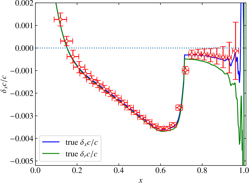
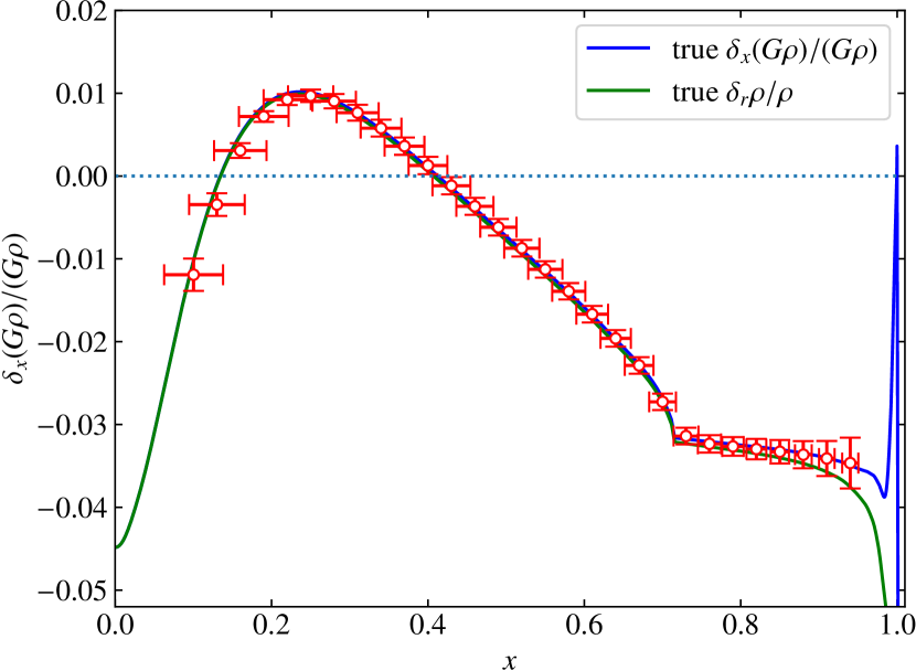
Figure 3: Test structure inversions based on two theoretical models (cf. Section 5). One is model S of Christensen-Dalsgaard et al. (1996), which is used as the reference model, while the other is model 1 of Houdek & Gough (2007), which is homologously shrunk by $0.01$ per cent. The inversions for $\delta_{x}c/c$ and $\delta_{x}(G\rho)/(G\rho)$ are shown in the left and right panels, respectively, as functions of the fractional radius $x$ of the reference model, which is normalized by the photospheric radius. In each panel, the red open circles with errorbars indicate the inversion results. The horizontal bars stand for the width of the averaging kernels, while the vertical errorbars stand for the statistical errors that originate from the uncertainties in frequencies, which are assumed to be the same as those of MDI 360-day data set. The blue curves denote the corresponding true differences; the green curves, which represent $\delta_{r}c/c$ and $\delta_{r}\rho/\rho$ in the left and right panels, respectively, are included for comparison.

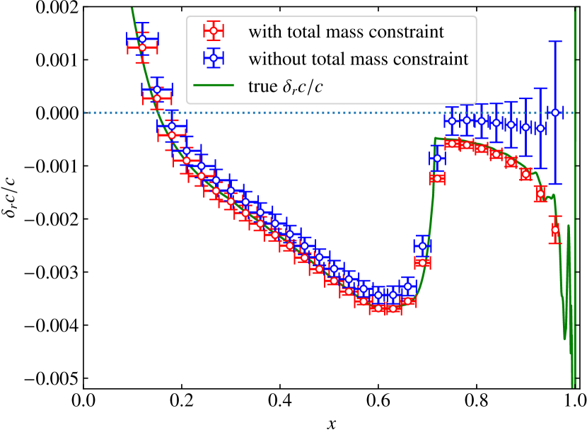
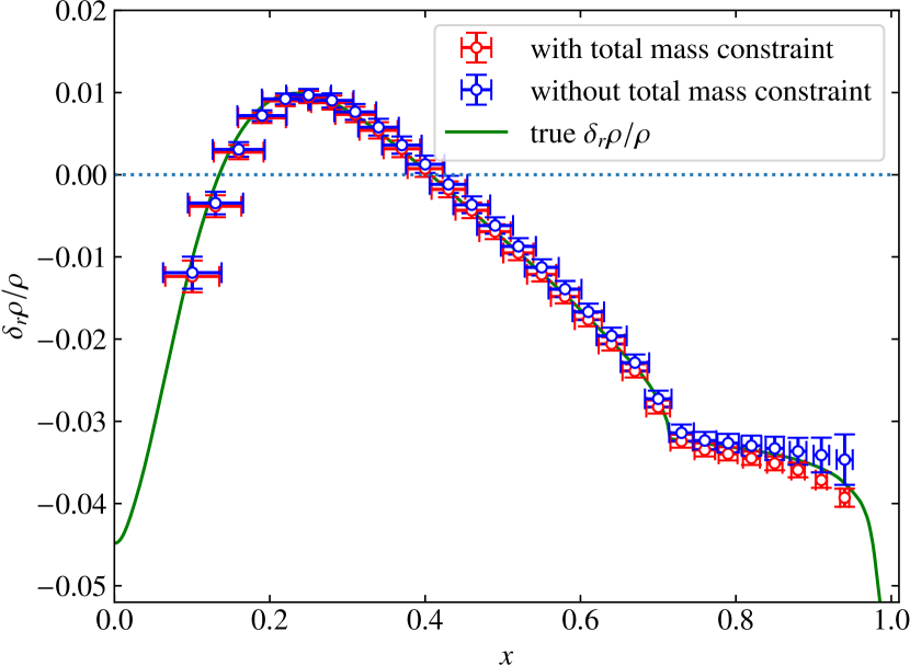
Figure 4: Test structure inversions by the conventional method, which does not consider the difference between the radii of target structure and the reference model. The target and reference models are the same as those in Fig. 3. The left and right panels show the sound speed and density differences, respectively, at fixed radius. The inversion results with (without) the total mass constraint are plotted by red (blue) open circles with errorbars, and the corresponding true differences are drawn by green curves. The meanings of the horizontal axes and the errorbars follow Fig. 3.

We validate the method of structure inversion, which is described in Sections 5.1 and 5.2, based on the same theoretical models as those in Section 6.3. We use all the p modes in the dataset, which is common with the MDI 360-day data, but exclude f modes. Fig. 3 shows the results of the inversions for $\delta_{x}c/c$ (left panel) and $\delta_{x}(G\rho)/(G\rho)$ (right panel). They are fully consistent with the true differences (drawn by blue curves) in the both cases. In the left panel, we observe that the values of $\delta_{x}c/c$ are nearly constant in the convective envelope ($x\gtrsim 0.7$), whereas the true difference of $\delta_{r}c/c$ (green curve) increases in magnitude towards the surface. This is the direct effect of scaling introduced in the inversion process. In fact, we understand from equation (29)

$$\frac{\delta_{x}c}{c}=\frac{\delta_{r}c}{c}+\frac{\delta R}{R}\frac{\text{d}\ln c}{\text{d}\ln r}\;.$$ (46)

The almost constant small values of $\delta_{x}c/c$ in the convection zone beneath the superadiabatic boundary layer implies that the second term on the right-hand side of equation (46) nearly cancels the first term (the green curve in Fig. 3). The corresponding difference in the density inversions can be understood similarly.

We then check any potential troubles in the conventional inversion method. In Fig. 4, we present the inversion results for $\delta_{r}c/c$ (left panel) and $\delta_{r}\rho/\rho$ (right panel) based on the conventional method. We assume that the target structure (shrunk model 1) has the same radius as the reference model (model S). Two cases with and without the total mass constraint are shown in each panel. The results for $\delta_{r}c/c$ with the total mass constraint (red points in the left panel) are consistent with the true difference (green curve). On the other hand, those without the total mass constraint (blue points) are systematically larger by $\sim 10^{-4}$ than the true curve (green) for $x\lesssim{0.7}$, whereas the difference becomes larger as $x$ increases for $x\gtrsim{0.7}$, and reaches $\sim 2\times 10^{-3}$ for $x=0.96$. These values are formally obtained by shifting upward the red points in the left panel of Fig. 3 by $10^{-4}$. This is because the conventional inversion for $\delta_{r}c/c$ without the total mass constraint should be reinterpreted as $\delta_{x}\psi/\psi=\delta_{x}c/c-\delta R/R$ (cf. Section 3.2).

The conventional inversions for $\delta_{r}\rho/\rho$ with the total mass constraint (red points in the right panel) are systematically smaller than the true values (green curve) by $\sim 10^{-3}$ for $x\gtrsim 0.7$. These differences could be understood as a nonlinear effect, which we may estimate to be of the order of $(\delta_{r}\rho/\rho)^{2}\sim(3\times 10^{-2})^{2}\sim 10^{-3}$ in the relevant range of $x$. On the contrary, the results without the total mass constraint (blue points) are larger than the true curve (green) by $\sim 10^{-3}$ for $x\gtrsim 0.8$. These results are numerically the same as those shown by red open circles in the right panel of Fig. 3 since $\delta_{r}\rho/\rho$ without the total mass constraint should be reinterpreted as $\delta_{x}(G\rho)/(G\rho)$ (cf. Section 3.2) .

7 Inversion of observational data

In this section, we apply the inversion methods developed in Sections 4.1, 5.1 and 5.2, for the radius, sound speed and density, respectively, to observational data. The frequency data set used in this paper was obtained from the SOI/MDI instrument on the SOHO spacecraft (Schou, 1999). We use all the p modes included in the available 360-day data. Again we adopt model S by Christensen-Dalsgaard et al. (1996) as the reference model.

We do not include f modes in the analysis. This is chiefly because p modes and f modes are sensitive to different radii as we discuss in Section 2. In addition, a complication arises from the fact that the surface terms for the two kinds of mode differ, because the characteristics of the modes are rather different, partly because f modes are uncompressed (cf. Section 4.1). Indeed, the functions $F_{0}$ and $F_{2}$ for p modes are inapplicable to f modes, because f-mode frequencies are intimately related to degree.

7.1 Structure inversion

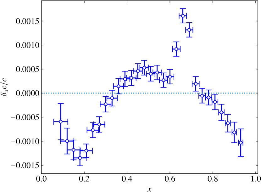
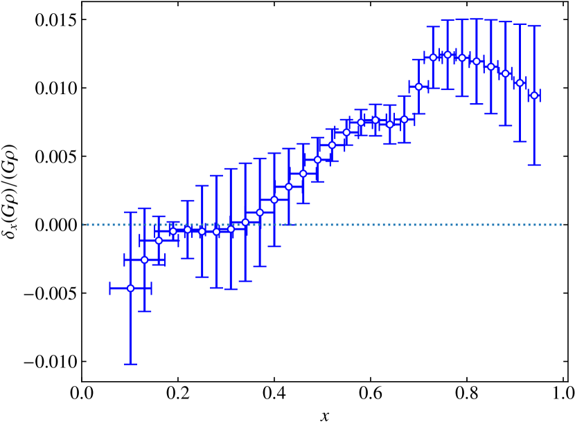
Figure 5: Inversions for the structure of the Sun based on the MDI 360-day data. The method is described in detail in Section 5. The results for the sound speed and the density multiplied by the gravitational constant are given in the left and right panels, respectively. The ordinate of each panel means the relative difference of the solar values from those of the reference model at the fixed fractional radius, $x$. The meanings of the horizontal bars and the vertical errorbars follow Fig. 3.

In the left panel of Fig. 5, sound-speed inversions obtained by the method described in Section 5.1 are presented. Since the claimed relative difference between the radii of the Sun and the standard solar model is of the order of $10^{-4}$ (Schou et al., 1997; Antia, 1998), its second-order effect on the new structure inversions is expected to be of the order of $10^{-8}$, which is small enough to be safely ignored at the current level of the accuracy of the eigenfrequency measurements. Unlike in the case of the test inversions in Section 6.4, $\delta_{x}c/c$ in the convective envelope increases in magnitude towards the surface. This implies that this region can be described by different scaling from what is adopted in these inversions, as we discuss in Section 8.1.

The corresponding density inversions are depicted in the right panel of Fig. 5. We observe that the values of $\delta_{x}(G\rho)/(G\rho)$ are mostly positive. This is understandable because we do not use the total mass constraint. As in the case of the sound-speed inversions, the values of $\delta_{x}(G\rho)/(G\rho)$ in the convective envelope tend to decrease towards the surface.

Table 4: Radius inversions using only the p modes. $\delta R$ is the estimated radius scale of the Sun minus the radius scale of the reference, model S. Parameters $n_{0}$ and $n_{2}$ denote the numbers of terms in the expansions of the surface-term functions $F_{0}$ and $F_{2}$ in equation (28), respectively; $\alpha_{R}$, $\beta_{R}$ and $\gamma_{R}$ are parameters in the formula (25) for $\chi^{2}_{R}$ whose minimization determines the coefficients $c_{n,l}$; in all the cases they are fixed at $\alpha_{R}=1$, $\beta_{R}=10^{2}$ and $\gamma_{R}=5\times 10^{7}$. In the inversions, it was assumed that $\delta(GM)/(GM)=0$ as described after equation (26), because the relative error in the measurement of $G\mbox{M}_{\sun}$ is on the order of $10^{-11}$ (see Table 1). An estimate of the error in ${(}\delta R/R{)_{\text{ac}}}$ is provided by $\sigma$; its value is rather ‘large’ as a result of a trade-off with the suppression of the contaminating integrals of equation (21) listed in the last two columns. Here, we define the cross-talk integrals $C_{\psi}:=\int\mathcal{K}^{{(R)}}_{\psi,\rho}\;\delta_{x}\psi/\psi\;\text{d}x$ and $C_{\rho}:=\int\mathcal{K}^{{(R)}}_{\rho,\psi}\;\delta_{x}(G\rho)/(G\rho)\;\text{d}x$.

$\begin{array}[]{cccccc}\hline\cr n_{0}&n_{2}&(\delta R/R)_{\text{ac}}&\sigma&C_{\psi}&C_{\rho}\\ \hline\cr 12&0&-4.3\times 10^{-4}&6\times 10^{-5}&-6\times 10^{-5}&-7\times 10^{-5}\\ 12&12&-3.1\times 10^{-4}&7\times 10^{-5}&-6\times 10^{-5}&-6\times 10^{-5}\\ 20&20&-3.5\times 10^{-4}&7\times 10^{-5}&-6\times 10^{-5}&-5\times 10^{-5}\\ 40&40&-3.1\times 10^{-4}&8\times 10^{-5}&-7\times 10^{-5}&-5\times 10^{-6}\\ \hline\cr\end{array}$

7.2 Radius inversion

We perform the radius inversion following the method in Section 4.1. Although the absolute values of the two integrals in equation (21) should be small enough not to affect the inversions, these terms could be sources of systematic error in the final answers given by equation (26). We estimate these integrals using the profiles of $\delta_{x}\psi/\psi$ and $\delta_{x}(G\rho)/(G\rho)$ obtained in the inversion without the total mass constraint (cf. Section 5). The results are given in Table 4.

In Table 4, we also check the sensitivity of the inversions to the numbers of terms included in the expansion of the surface-term functions $F_{0}$ and $F_{2}$, which we denote by $n_{0}$ and $n_{2}$, respectively. We see that the results are insensitive to both $n_{0}$ and $n_{2}$, provided they both exceed 12. We adopt the last entry in Table 4 as the final answer of the present study. To be conservative, we regard the 3-$\sigma$ level of the formal error as the uncertainty in the current estimate of the radius difference between the Sun and the reference model. Hence we estimate that $(\delta R/R)_{\text{ac}}=(-3.1\pm 2.4)\times 10^{-4}$. Combining this with equations (1) and (40), we obtain the p-scaled (photospheric) radius as $\mbox{R}_{\text{p}}=695.78\pm 0.16~{}\text{Mm}$. Recall that, strictly speaking, this result depends on assuming a homologous difference in the structure of the outer layers of the Sun beyond the upper turning point of the p modes included in the present study. Here, we have used the photospheric radius of the reference model, ${\mbox{R}_{\text{ph,r}}=}695.99~{}\text{Mm}$.

8 Discussion

Although Schou et al. (1997) analysed f-mode frequencies to give ${\mbox{R}_{\text{f}}}=695.68\pm 0.03$ Mm, the errors are dominated by the systematic errors. The corresponding 3-$\sigma$ statistical errors are estimated to be $0.02$ Mm. Although their estimate has a smaller formal error than ours, their result may be sensitive to the description of the subsurface layer of superadiabatic convection, as they point out themselves. On the other hand, our analysis is expected to be almost free from that ambiguity, partly because we have used p modes which are evanescent in the most turbulent region of the convection zone and partly because we have taken account of as many as 40 terms in the expansion of the surface term, which is expected to remove the uncertainty concerning the subsurface structure to a considerable extent. Dziembowski et al. (2000) also analysed f-mode data, implying the relative difference between the f-mode radii of the Sun and model S (Christensen-Dalsgaard et al., 1996) of ${\delta\mbox{R}_{\text{f}}/\mbox{R}_{\text{f}}}=(-4.52\pm 0.03)\times 10^{-4}$ ($\pm$ one standard deviation), averaged over nearly 3 years; the major variation in $\mbox{R}_{\text{f}}$ appears to be an oscillation with a 1-year period, which may suggest a susceptibility of the analysis at the $10^{-5}$ level to an annual variation in the SOHO–Sun distance resulting from, for example, pixel quantization or instrumental temperature variations, not to mention genuine solar-cycle radius variation of the Sun.

Alternatively, Antia (2003) claims that the apparent time-variation of the f-scaled radius could have been caused by a change in the MDI/SOI instrument during the few-months ‘vacation’ of the SOHO spacecraft in 1998 and 1999. Subsequently, Lefebvre & Kosovichev (2005) and Lefebvre et al. (2007) studied the nonhomologous solar-cycle variation of the subsurface layers based on the f-mode frequencies. Rozelot et al. (2018) have reported another interesting result: the f-mode frequencies are correlated with sunspot numbers over nearly two cycles ($\sim 22$ years).

We find that the central value of our radius inversion lies between the two direct observations quoted by Allen (1973) and Brown & Christensen-Dalsgaard (1998), though the former of them is consistent with our result at the 3-$\sigma$ level of the error.

8.1 Sound-speed inversions in the convective envelope

We observe in the left panel of Fig. 5 that the sound-speed inversions for $x\gtrsim 0.7$ decrease monotonically towards the surface. It is well established that this region is composed of essentially adiabatically stratified layers, in which $p=K\rho^{\gamma_{1}}$ with constant $K$. The sound speed is then approximately described by

$$c^{2}\approx\left(\gamma_{1}-1\right)G\mbox{M}_{\sun}\left(\frac{1}{r}-\frac{1}{\mbox{R}_{\text{s}}}\right)\;,$$ (47)

which can be derived from the equations of hydrostatic equilibrium under the assumptions of constant $\gamma_{1}$ and constant mass enclosed within radius $r$. Here $\mbox{R}_{\text{s}}$ is the location of the phantom singularity that was introduced in Section 2. The expression for $\delta_{x}c/{c}$ can be derived from equation (47) as

$$\frac{\delta_{x}c}{c}\approx\frac{1}{2}\left({\frac{\delta\gamma_{1}}{\gamma_{1}-1}}-\frac{\delta R}{R}\right)-\frac{1}{2\mbox{R}_{\text{s}}}\left(\frac{\delta R}{R}-\frac{\delta\mbox{R}_{\text{s}}}{\mbox{R}_{\text{s}}}\right)\left(\frac{1}{r}-\frac{1}{\mbox{R}_{\text{s}}}\right)^{-1}\;.$$ (48)

The growing trend in the sound-speed inversions can be interpreted as a contribution from the second term on the right-hand side of equation (48). Comparing the approximate relation (48) with a more accurate expression,

$$\frac{\delta_{x}c}{c}=\frac{\delta_{x_{\text{s}}}c}{c}+\left(\frac{\delta R}{R}-\frac{\delta\mbox{R}_{\text{s}}}{\mbox{R}_{\text{s}}}\right)\frac{\text{d}\ln c}{\text{d}\ln r}\;,$$ (49)

in which $x_{\text{s}}=r/\mbox{R}_{\text{s}}$, we may regard the first term on the right-hand side of equation (49) as being almost constant, as one might expect. Fitting equation (49) to the sound-speed inversion performed in Section 7.1, we estimate, in particular,

$$\frac{\delta\mbox{R}_{\text{s}}}{\mbox{R}_{\text{s}}}-\left(\frac{\delta R}{R}\right)_{\text{ac}}\approx{-0.0003}\;.$$ (50)

This means that the position of the adiabatically stratified layers, which is characterized by $\mbox{R}_{\text{s}}$, is located about $0.06$ per cent deeper in the Sun than in model S, whereas $\mbox{R}_{{\text{ac}}}$, which is almost equal to the photospheric radius, is smaller by only $0.03$ per cent. The result of $\delta\mbox{R}_{\text{s}}/\mbox{R}_{\text{s}}\neq{(}\delta R/R{)_{\text{ac}}}$ means that the difference between the Sun and model S is not homologous for $x\gtrsim 0.7$. This information would be useful for our better understanding of the structure of the upper convective layers in the Sun.

8.2 Remark on Basu

Basu (1998) performed conventional structure inversions using two different reference models, one with the standard value of the photospheric radius, $695.99$ Mm, the other with the smaller radius ${\mbox{R}_{\text{ph}}}=695.78$ Mm. She found a significant difference between the results, both in the sound-speed and in the density inversions. Her demonstrations emphasize that so long as we adhere to conventional inversions we must take care in interpreting the results. On the other hand, by extending the inversion formulae so as to take account of the uncertainties in the solar radius $\mbox{R}_{\sun}$ and the product $G\mbox{M}_{\sun}$ of the gravitational constant and the solar mass, we have succeeded in carrying out inversions that are independent of the radius differences (at least in the leading order). Note that the uncertainty in $G\mbox{M}_{\sun}$ can be neglected in practice because it is much smaller than the errors in frequencies provided by current observations. We can say that our method gives conservative answers, in the sense that it makes the results independent of the uncertainties in the radius $R$ at the expense of greater formal errors.

8.3 Uncertainty in the gravitational constant

In principle, the density inversions are affected by any error $\sigma_{G}$ in the gravitational constant, which is of the order of $10^{-5}$ (cf. Table 1), although the formal errors in the right panel of Fig. 5 are larger by about two orders of magnitude. Similarly, if there were a difference in the gravitational constant $G$ between the Sun and the reference model, then the density inversions should be shifted by a constant $\delta G/G$ since

$$\frac{\delta_{x}\rho}{\rho}=\frac{\delta_{x}(G\rho)}{G\rho}-\frac{\delta G}{G}\;.$$ (51)

8.4 Relation to asteroseismology

It is worth thinking about the application of the present technique to the field of asteroseismology (cf. Gough & Kosovichev, 1993; Reese et al., 2012; Buldgen et al., 2019). The present method enables us to perform the structure inversions that are independent of the uncertainties in the total radius $R$ if we know the product $GM$ of the gravitational constant and the total mass of the target star accurately. If $GM$ were not accurately known, but the radius $R$ of the star were measured, for example, by the interferometric observations (e.g. Kervella et al., 2004), it would still be possible to perform the inversions for the structure difference and the total mass difference (if frequencies were available for a large variety of oscillation modes). In fact, the inversions for $\delta_{x}\psi/\psi$ and $\delta_{x}(G\rho)/(G\rho)$ can be accomplished using only equation (3), as is explained in Section 3.3. In this case, we do not have to worry about any ambiguity in the definition of the operator $\delta_{x}$ since the radius difference is known. Then the mass difference $\delta(GM)/(GM)$ can be inferred by another OLA-type inversion that utilizes the total mass constraint given by equation (6). If, in the worst case, we know neither $R$ nor the product $GM$ of the target star, we can estimate only the difference in $GM/R^{3}$ by a procedure similar to that described above. A reliable estimate of the surface gravity $GM/R^{2}$ by spectroscopy (or the theoretical mass-radius relation) then constrains both of the radius and the mass of the target star. These days, the mass and radius of solar-like oscillators are often estimated from the large frequency separation, $\Delta\nu$, and the frequency of maximum power, $\nu_{\max}$, based on the scaling relations.

Once the radius difference is known, the structure differences $\delta_{x}\psi/\psi$ and $\delta_{x}(G\rho)/(G\rho)$, which are inferred by equation (3), can be defined without ambiguity.

8.5 The case of the large radius difference

We note in passing that the assumption that $\delta R/R$ is small is not actually essential, though it is implicitly made when we write down equation (29). In fact, we can carry out a similar analysis even when $\delta R/R$ is not small, provided that the structure difference is nearly homologous. Here the nearly homologous difference means that the differences at fixed fractional radius in the dimensionless variables

$$\tilde{\psi}:=\sqrt{\frac{R^{3}}{GM}}\,\psi$$ (52)

and

$$\tilde{\rho}:=\frac{R^{3}}{M}\,\rho$$ (53)

can be made small by adjusting the radius (scale factor) of the target structure. Let us denote the radii $R$ of the reference model and the target structure by $\mbox{R}_{\text{r}}$ and $\mbox{R}_{\text{t}}$, respectively. In this section, subscripts r and t generally mean the quantities of the reference model and the target structure, respectively. We do not assume $\left|\mbox{R}_{\text{t}}-\mbox{R}_{\text{r}}\right|\ll\mbox{R}_{\text{r}}$. We first set $\mbox{R}_{\text{t}}=\mbox{R}_{\text{t},0}$, for which the corresponding difference operator at fixed radius is denoted by $\delta_{x,0}$. The value of $\mbox{R}_{\text{t},0}$ can be chosen arbitrary so long as $\delta_{x,0}\tilde{\psi}$ and $\delta_{x,0}\tilde{\rho}$ are small. We then consider variation in $\mbox{R}_{\text{t}}$ as $\mbox{R}_{\text{t}}=\mbox{R}_{\text{t},0}+\delta\mbox{R}_{\text{t}}$, in which we assume $\left|\delta\mbox{R}_{\text{t}}\right|\ll\mbox{R}_{\text{t},0}$. The corresponding difference operator at fixed fractional radius is denoted by $\delta_{x}$. After these preparations, we may repeat the analysis in Section 4.3, but with $\psi$, $G\rho$, $\delta R/R$ and $\delta_{r}$ replaced by $\tilde{\psi}$, $\tilde{\rho}$, $\delta\mbox{R}_{\text{t}}/\mbox{R}_{\text{t},0}$ and $\delta_{x,0}$. Equation (38), in particular, is reduced to

$$\frac{\delta\mbox{R}_{\text{t}}}{\mbox{R}_{\text{t},0}}=\lim_{x_{0}\rightarrow x_{{\text{surf}}}}\frac{\displaystyle\frac{\delta_{x,0}\tilde{\rho}}{\tilde{\rho}_{\text{r}}}(x_{0})}{\displaystyle-\frac{{\text{d}}\ln\rho_{\text{r}}}{{\text{d}}\ln r}(x_{0})}\;,$$ (54)

which is equivalent to

$$\lim_{x_{0}\rightarrow x_{{\text{surf}}}}\frac{\displaystyle\frac{\delta_{x}\tilde{\rho}}{\tilde{\rho}_{\text{r}}}(x_{0})}{\displaystyle-\frac{{\text{d}}\ln\rho_{\text{r}}}{{\text{d}}\ln r}(x_{0})}=0\;.$$ (55)

We can easily understand how the scale factor $\mbox{R}_{\text{t}}$ is included in equation (55) by remembering that

$$\delta_{x}\tilde{\rho}(x)=\frac{\mbox{R}_{\text{t}}^{3}}{\mbox{M}_{\text{t}}}\,\rho_{\text{t}}\left(x\mbox{R}_{\text{t}}\right)-\frac{\mbox{R}_{\text{r}}^{3}}{\mbox{M}_{\text{r}}}\,\rho_{\text{r}}\left(x\mbox{R}_{\text{r}}\right)\;.$$ (56)

The scale factor $\mbox{R}_{\text{t}}$, which can be very different from $\mbox{R}_{\text{r}}$, is identified as the zero point of the left-hand side of equation (55), regarded as a function of $\mbox{R}_{\text{t}}$. That, of course, is provided that the target and the reference have essentially the same outer atmospheres, as is the case for the models studied in Section 6.2. This analysis, which allows for a large radius difference, must be of use when we think about inversions of stars other than the Sun, whose radii we often do not know well.

9 Conclusion

In this paper, we have extended the inversion formulae to consider the difference in the radii of the reference model and the Sun. We have performed inversions for the radius of the Sun, and estimate the solar photospheric radius (which we quote with 3-$\sigma$ statistical errors) to be $695.78\pm 0.16~{}\text{Mm}$ from only p-mode frequencies. We have also performed structure inversions for the sound-speed and density profiles of the Sun independently of the uncertainties in the solar radius. The sound-speed inversion suggests that the positions of the photosphere and the adiabatically stratified layers in the convective envelope differ nonhomologously from those of the standard solar model.

Data availability

The data underlying this article will be shared on reasonable request to the corresponding author.

Appendix A Derivation of the inversion formulae

Here we derive equation (3) for the fractional difference $\delta\nu_{n,l}/\nu_{n,l}$ between the solar frequencies and the eigenfrequencies of a reference model in terms of the corresponding structural differences in sound speed and density. First, we introduce the dimensionless variables,

$$\tilde{\nu}_{n,l} :=\sqrt{\frac{R^{3}}{GM}}\;\nu_{n,l}\;,$$ (57)

$$\tilde{c} :=\sqrt{\frac{R}{GM}}\;c$$ (58)

$$\tilde{\rho} :=\frac{R^{3}}{M}\;\rho\;.$$ (59)

The equations of hydrostatic equilibrium and mass conservation can be rewritten in terms of these dimensionless variables, and are quite similar to the original forms. With these equations, the derivation of the kernels for dimensionless sound-speed $\tilde{c}$ and dimensionless density $\tilde{\rho}$ is parallel to that for the dimensional variables, for which readers can refer, for example, to the article by Gough & Thompson (1991). The difference is that we should compare the variables at the fixed fractional radius $x=r/R$ instead of the fixed absolute radius $r$. The resulting integral expression is

$$\frac{\delta\tilde{\nu}_{n,l}}{\tilde{\nu}_{n,l}}=\int K_{\tilde{c},\tilde{\rho}}^{(n,l)}\,\frac{\delta_{x}\tilde{c}}{\tilde{c}}\;\text{d}x+\int K_{\tilde{\rho},\tilde{c}}^{(n,l)}\,\frac{\delta_{x}\tilde{\rho}}{\tilde{\rho}}\;\text{d}x+S_{n,l}\;,$$ (60)

where $S_{n,l}$ is introduced to accommodate the uncertain physics in the near-surface layers of the star. It is therefore only very weakly dependent on the degree $l$ of the mode. The reason for this is because the ray paths of the high-order p modes are nearly vertical in the near-surface layers, irrespective of degree. Noting that the kernels for the dimensional variables are dimensionless, we can easily appreciate that

$$K_{\tilde{c},\tilde{\rho}}^{(n,l)}=K_{c,\rho}^{(n,l)}\;\;\;\;\;{\text{and}}\;\;\;\;\;K_{\tilde{\rho},\tilde{c}}^{(n,l)}=K_{\rho,c}^{(n,l)}:$$ (61)

the kernels for the dimensionless variables are identical to those for the dimensional variables. Note that equation (60) holds even for the case in which the real Sun and the reference model have different radii.

We next rewrite equation (60) in terms of the dimensional variables by using the definitions (57), (58) and (59):

$$\displaystyle\frac{\delta\tilde{\nu}_{n,l}}{\tilde{\nu}_{n,l}} =\frac{\delta\nu_{n,l}}{\nu_{n,l}}+\frac{3}{2}\,\frac{\delta R}{R}-\frac{1}{2}\,\frac{\delta(GM)}{GM}\;,$$ (62)

$$\displaystyle\frac{\delta_{x}\tilde{c}}{\tilde{c}} =\frac{\delta_{x}c}{c}+\frac{1}{2}\,\frac{\delta R}{R}-\frac{1}{2}\,\frac{\delta(GM)}{GM}$$ (63)

$$\displaystyle\frac{\delta_{x}\tilde{\rho}}{\tilde{\rho}} =\frac{\delta_{x}(G\rho)}{G\rho}+3\frac{\delta R}{R}-\frac{\delta(GM)}{GM}\;.$$ (64)

Introducing these relations together with equation (61) into equation (60) yields

$$\displaystyle\frac{\delta\nu_{n,l}}{\nu_{n,l}}= \int K_{c,\rho}^{(n,l)}\,\frac{\delta_{x}c}{c}\;\text{d}x+\int K_{\rho,c}^{(n,l)}\,\frac{\delta_{x}(G\rho)}{G\rho}\;\text{d}x$$

$$\displaystyle\mbox{}+\frac{\delta R}{R}\left(\frac{1}{2}\int K_{c,\rho}^{(n,l)}\;\text{d}x+3\int K_{\rho,c}^{(n,l)}\;\text{d}x-\frac{3}{2}\right)$$

$$\displaystyle\mbox{}-\frac{\delta(GM)}{GM}\left(\frac{1}{2}\int K_{c,\rho}^{(n,l)}\;\text{d}x+\int K_{\rho,c}^{(n,l)}\;\text{d}x-\frac{1}{2}\right)$$

$$\displaystyle\mbox{}+S_{n,l}\;.$$ (65)

We can go further by comparing equation (65) with the corresponding formula used for the conventional inversion, which is a particular case of equation (60):

$$\frac{\delta\nu_{n,l}}{\nu_{n,l}}=\int K_{c,\rho}^{(n,l)}\,\frac{\delta_{r}c}{c}\;\text{d}x+\int K_{\rho,c}^{(n,l)}\,\frac{\delta_{r}\rho}{\rho}\;\text{d}x+S_{n,l}\;.$$ (66)

We now emphasize that we must be able to recover equation (66) from equation (65), which is more general. To do so, all we need should be only to set $\delta G=0$ and $\delta R=0$ (hence $\delta_{x}=\delta_{r}$), because equation (66) has been derived without assuming $\delta M=0$. However, it is found that the substitution of those two conditions into equation (65), and the replacement of $\delta_{x}$ by $\delta_{r}$, are not sufficient to recover equation (66) unless the terms multiplying ${\delta(GM)}/{GM}$ cancel. In other words, the identity

$$\frac{1}{2}\int K_{c,\rho}^{(n,l)}\;\text{d}x+\int K_{\rho,c}^{(n,l)}\;\text{d}x=\frac{1}{2}\;,$$ (67)

must be satisfied for all $(n,l)$. From a physical point of view, equation (67) reflects the following homologous relation of the adiabatic oscillations of stars: if we multiply both the squared sound-speed profile and the density profile of a stellar model by the same constant factor, keeping their shapes fixed as functions of the fractional radius $x$, all of the squared eigenfrequencies change by the same factor. Using identity (67), equation (65) can be written

$$\displaystyle\frac{\delta\nu_{n,l}}{\nu_{n,l}}= \int K_{c,\rho}^{(n,l)}\,\frac{\delta_{x}c}{c}\;\text{d}x+\int K_{\rho,c}^{(n,l)}\,\frac{\delta_{x}(G\rho)}{G\rho}\;\text{d}x$$

$$\displaystyle\mbox{}-\frac{\delta R}{R}\int K_{c,\rho}^{(n,l)}\;\text{d}x+S_{n,l}\;.$$ (68)

This equation is identical to the following more compact expressions:

$$\frac{\delta\nu_{n,l}}{\nu_{n,l}}=\int K_{c,\rho}^{(n,l)}\,\frac{\delta_{x}(c/R)}{c/R}\;\text{d}x+\int K_{\rho,c}^{(n,l)}\,\frac{\delta_{x}(G\rho)}{G\rho}\;\text{d}x+S_{n,l}$$ (69)

and, more pertinently,

$$\frac{\delta\nu_{n,l}}{\nu_{n,l}}=\int K_{c,\rho}^{(n,l)}\,\frac{\delta_{x}\psi}{\psi}\;\text{d}x+\int K_{\rho,c}^{(n,l)}\,\frac{\delta_{x}(G\rho)}{G\rho}\;\text{d}x+S_{n,l}\;,$$ (70)

which follows by noticing the relation,

$$\frac{\delta_{x}r}{r}=\frac{\delta_{x}(Rx)}{Rx}=\frac{\delta R}{R}\;.$$ (71)

Equation (70) implies $K_{\psi,\rho}^{(n,l)}=K_{c,\rho}^{(n,l)}$ and $K_{\rho,\psi}^{(n,l)}=K_{\rho,c}^{(n,l)}$ in equation (3); neither contains the radius difference $\delta R$ explicitly.

Appendix B Derivation of the annihilator relation

Associate with a single structure two different scale factors $R$ and $R^{\prime}$. Let us call the structure with scale factor $R$ model A and that with $R^{\prime}$ model B. The difference in the scale factors is given by

$$\delta R:=R^{\prime}-R\;\neq 0.$$ (72)

To relate the radius $r$ in model A and radius $r^{\prime}$ in model B at the same fractional radius, we set

$$r^{\prime}/R^{\prime}=r/R\;,$$ (73)

from which

$$r^{\prime}=\frac{R^{\prime}}{R}\;r=\left(1+\frac{\delta R}{R}\right)r\;.$$ (74)

Therefore the difference between models A and B in any quantity $f$ at the same fractional radius $x$ is estimated as

$$\delta_{x}f:=f(r^{\prime})-f(r)=\frac{\delta R}{R}\;\frac{{\text{d}}f}{{\text{d}}r}\;r=\frac{\delta R}{R}\;\frac{{\text{d}}f}{{\text{d}}\ln r}\;,$$ (75)

which is valid in the linear regime. Hence we have

$$\frac{\delta_{x}f}{f}=\frac{\delta R}{R}\;\frac{{\text{d}}\ln f}{{\text{d}}\ln r}\;.$$ (76)

Using this formula, equation (3) reduces to

$$\frac{\delta\nu_{nl}}{\nu_{nl}} =\frac{\delta R}{R}\left(\int K_{\psi,\rho}^{(n,l)}\;\frac{{\text{d}}\ln\psi}{{\text{d}}\ln r}\;\text{d}x+\int K_{\rho,\psi}^{(n,l)}\;\frac{{\text{d}}\ln\rho}{{\text{d}}\ln r}\;\text{d}x\right)$$

$$\phantom{=}\mbox{}+S_{nl}\;,$$ (77)

where we have used

$$\frac{{\text{d}}\ln(G\rho)}{{\text{d}}\ln r}=\frac{{\text{d}}\ln\rho}{{\text{d}}\ln r}\;,$$ (78)

because $G$ is constant. Since the two structures are physically the same, we necessarily have $\delta\nu_{nl}/\nu_{nl}=0$, and we can ignore the surface term. Furthermore, because $\delta R/R\neq 0$, we obtain

$$0=\int K_{\psi,\rho}^{(n,l)}\;\frac{{\text{d}}\ln\psi}{{\text{d}}\ln r}\;\text{d}x+\int K_{\rho,\psi}^{(n,l)}\;\frac{{\text{d}}\ln\rho}{{\text{d}}\ln r}\;\text{d}x\;,$$ (79)

for any $(n,\,l)$, which is equation (7). Strictly speaking, we can show that equation (79) is correct only if $K_{\rho,\psi}^{(n,l)}=0$ at the surface.

Like equation (70), equation (79) is directly related to the homology relation explained in the main text that adiabatic eigenfrequencies are invariant under uniform stretching in the radial direction and appropriate scaling of the structure.

Appendix C Inversion formulae and kernel identities for various inversion variables

In the discussion in the body of the paper we have adopted the sound speed $c$ and density $\rho$ for inversion variables. In a manner analogous to that in Appendices A and B, we can derive corresponding formulae and identities for any other seismologically independent pair of structure variables. The procedure is summarized in this subsection. The outcome is useful not only for helioseismological inversion, but also when we study the seismological inversion for the structure of other stars (cf. Gough & Kosovichev, 1993; Takata & Montgomery, 2002), in which case we usually do not know the precise values of the mass and radius. The kernels for variables other than $c$ and $\rho$ can be obtained by the method described by Gough (1996). For brevity we now omit the surface term in the inversion formulae

C.1 Density and first adiabatic exponent

If we choose the density $\rho$ and the first adiabatic exponent $\gamma_{1}$ as inversion variables, we have

$$\frac{\delta\nu_{n,l}}{\nu_{n,l}}=\int K_{\rho,\gamma_{1}}^{(n,l)}\frac{\delta_{x}(G\rho)}{G\rho}\;\text{d}x+\int K_{\gamma_{1},\rho}^{(n,l)}\frac{\delta_{x}\gamma_{1}}{\gamma_{1}}\;\text{d}x\,.$$ (80)

With this variable pair, terms explicitly containing the difference in mass or radius that might have arisen in the derivation of the kernels cancel out, as is the case in the derivation of equation (3). We need pay attention only to the fact that the difference between the reference model and the target should be taken not at the fixed absolute radius $r$ but at fixed fractional radius $x$, whose definition implicitly includes the radius $R$. Essentially the same discussion as that in Appendix A leads us to the identity,

$$\int K_{\rho,\gamma_{1}}^{(n,l)}\;\text{d}x=\frac{1}{2}\;,$$ (81)

which corresponds to equation (67); the annihilator relation,

$$\int K_{\rho,\gamma_{1}}^{(n,l)}\frac{{\text{d}}\ln\rho}{{\text{d}}\ln r}\;\text{d}x+\int K_{\gamma_{1},\rho}^{(n,l)}\frac{{\text{d}}\ln\gamma_{1}}{{\text{d}}\ln r}\;\text{d}x=0\;,$$ (82)

is obtained by the same scaling argument as that given in Appendix B. Equation (81) is equivalent to equation (14) of Reese et al. (2012).

C.2 Adiabatic sound-speed and first adiabatic exponent

When $c^{2}$ and the first adiabatic exponent $\gamma_{1}$ are adopted as inversion variables, the integral formula for the relative frequency perturbation is revised as follows:

$$\frac{\delta\nu_{n,l}}{\nu_{n,l}} =\int K_{c^{2},\gamma_{1}}^{(n,l)}\frac{\delta_{x}\psi^{2}}{\psi^{2}}\;\text{d}x+\int K_{\gamma_{1},c^{2}}^{(n,l)}\frac{\delta_{x}\gamma_{1}}{\gamma_{1}}\;\text{d}x$$

$$\phantom{=}\mbox{}+\left(\frac{1}{2}-\int K_{c^{2},\gamma_{1}}^{(n,l)}\;\text{d}x\right)\left(\frac{\delta(GM)}{GM}-3\,\frac{\delta R}{R}\right)\;,$$ (83)

which corresponds to equation (65). In equation (83), we have used $K_{\psi^{2},\gamma_{1}}^{(n,l)}=K_{c^{2},\gamma_{1}}^{(n,l)}$ and $K_{\gamma_{1},\psi^{2}}^{(n,l)}=K_{\gamma_{1},c^{2}}^{(n,l)}$. There are two new terms on the right-hand side to take account of the mass and radius differences. Applying the scaling discussed in Appendix B leads to the analogue of equation (79):

$$\int K_{c^{2},\gamma_{1}}^{(n,l)}\left(\frac{{\text{d}}\ln c^{2}}{{\text{d}}\ln r}+1\right)\;\text{d}x+\int K_{\gamma_{1},c^{2}}^{(n,l)}\frac{{\text{d}}\ln\gamma_{1}}{{\text{d}}\ln r}\;\text{d}x=\frac{3}{2}\,.$$ (84)

We have only one kind of kernel identity in this case because the coefficient of the mass difference does not vanish in equation (83), unlike the case in which $c$ and $\rho$ are adopted as inversion variables. This is, in turn, because we need to assume the total mass constraint to derive the expressions for $K_{c^{2},\gamma_{1}}^{(n,l)}$ and $K_{\gamma_{1},c^{2}}^{(n,l)}$ (e.g. Gough, 1996).

C.3 Isothermal sound-speed and first adiabatic-exponent

We consider the case where the inversion variables are set to the isothermal sound-speed, $u:=p/\rho$, and the first adiabatic exponent $\gamma_{1}$. Substituting the trivial relations, $K_{c^{2},\gamma_{1}}^{(n,l)}=K_{u,\gamma_{1}}^{(n,l)}$ and $K_{\gamma_{1},c^{2}}^{(n,l)}=K_{\gamma_{1},u}^{(n,l)}-K_{u,\gamma_{1}}^{(n,l)}$, into equations (83) and (84), yields

$$\frac{\delta\nu_{n,l}}{\nu_{n,l}} =\int K_{u,\gamma_{1}}^{(n,l)}\frac{\delta_{x}(u/r^{2})}{u/r^{2}}\;\text{d}x+\int K_{\gamma_{1},u}^{(n,l)}\frac{\delta_{x}\gamma_{1}}{\gamma_{1}}\;\text{d}x$$

$$\phantom{=}\mbox{}+\left(\frac{1}{2}-\int K_{u,\gamma_{1}}^{(n,l)}\;\text{d}x\right)\left(\frac{\delta(GM)}{GM}-3\,\frac{\delta R}{R}\right)$$ (85)

and

$$\int K_{u,\gamma_{1}}^{(n,l)}\left(\frac{{\text{d}}\ln u}{{\text{d}}\ln r}+1\right)\;\text{d}x+\int K_{\gamma_{1},u}^{(n,l)}\frac{{\text{d}}\ln\gamma_{1}}{{\text{d}}\ln r}\;\text{d}x=\frac{3}{2}\;,$$ (86)

respectively.

We finally make a remark about the difference between $c^{2}$ and $u$. Since the analyses in Appendices C.2 and C.3 are essentially the same, it might possibly be accepted that it makes little difference whether we choose $c^{2}$ or $u$ as one of the inversion variables. This is, however, not always true. As pointed out by Däppen et al. (1991), for example, when combined with the helium mass fraction $Y$, $u$ is usually preferred over $c$ or $c^{2}$ for the accompanying inversion variable because it avoids putative divergences in the $c^{2}$ kernel in ionization zones of abundant elements at locations where $(\partial{\rm ln}\gamma_{1}/\partial{\rm ln}\rho)_{p,Y}=1$, thereby obviating unnecessary mathematical complication.

References

- Allen (1973) Allen C. W., 1973, Astrophysical quantities, 3rd edn. Athlone Press, London
- Antia (1998) Antia H. M., 1998, A&A, 330, 336
- Antia (2003) Antia H. M., 2003, ApJ, 590, 567
- Antia et al. (2000) Antia H. M., Basu S., Pintar J., Pohl B., 2000, Sol. Phys., 192, 459
- Backus & Gilbert (1968) Backus G., Gilbert F., 1968, Geophysical Journal, 16, 169
- Balmforth & Gough (1990) Balmforth N. J., Gough D. O., 1990, ApJ, 362, 256
- Basu (1998) Basu S., 1998, MNRAS, 298, 719