Humanising robot-assisted navigation

Abstract

Robot-assisted navigation is a perfect example of a class of applications requiring flexible control approaches. When the human is reliable, the robot should concede space to their initiative. When the human makes inappropriate choices the robot controller should kick-in guiding them towards safer paths. Shared authority control is a way to achieve this behaviour by deciding online how much of the authority should be given to the human and how much should be retained by the robot. An open problem is how to evaluate the appropriateness of the human’s choices. One possible way is to consider the deviation from an ideal path computed by the robot. This choice is certainly safe and efficient, but it emphasises the importance of the robot’s decision and relegates the human to a secondary role. In this paper, we propose a different paradigm: a human’s behaviour is correct if, at every time, it bears a close resemblance to what other humans do in similar situations. This idea is implemented through the combination of machine learning and adaptive control. The map of the environment is decomposed into a grid. In each cell, we classify the possible motions that the human executes. We use a neural network classifier to classify the current motion, and the probability score is used as a hyperparameter in the control to vary the amount of intervention. The experiments collected for the paper show the feasibility of the idea. A qualitative evaluation, done by surveying the users after they have tested the robot, shows that the participants preferred our control method over a state-of-the-art visco-elastic control.

1 Introduction

We are living a time when robots are no longer confined to industrial environments but are used in numerous applications that require an unprecedented degree of autonomy. Modern robots have to adapt to humans, to understand their needs and help them carry out their activities. It is easy to predict a future in which the interaction between robots and humans will draw a direct inspiration from the rider-horse metaphor [1], with the human having developed an “innate” ability to use the robot’s services, and the robot being able to grasp the human’s intention without any explicit request.

In this paper we consider a use case in which the FriWalk robotic rollator (see Fig. 1-a), a robotic assistant able to localise itself in complex environments and generate safe routes, is used as navigation and walking support for a person with mild cognitive deficits. We consider the case of users with mild cognitive deficits, who could find it difficult to plan and follow long paths across complex and populated environments. These conditions could generate stress and fatigue and determine a gradual withdrawal of the user from the public space. A moderate cognitive support implemented by a system that gently guides the user can play a useful role in recovering or preserving the user’s sense of direction and her/his cognitive abilities. Since our ultimate goal is to prolong and promote the human’s autonomy, the system seeks to leave the human in control of the guidance as much as possible taking over the trajectory control only when the human’s actions are evidently flawed. This is a specific paradigm of a more general idea dubbed shared authority control, in which the robot is moved partly by the human and partly by the autonomous system, based on the contingent situation. In our previous work [2], we developed a guidance system of this kind based on a hybrid control scheme. In that study, the system leaves the user in control or kicks in the automatic guidance based on safety considerations. This is a remarkable simplification of the design space: the amount of authority reserved to the guidance system is increased when the distance from the border of a safe virtual corridor becomes too narrow. Similarly in [3] the shift in authority is based on the localisation accuracy. The reference trajectory can be found by the use of optimal path planning algorithms, even for dynamic scenarios [4].

The previous paradigms used a robot-centric and, to some extent, patronising point-of-view: the ideal behaviour is one where the human would do exactly the same things that the robot has planned through optimal path planning.

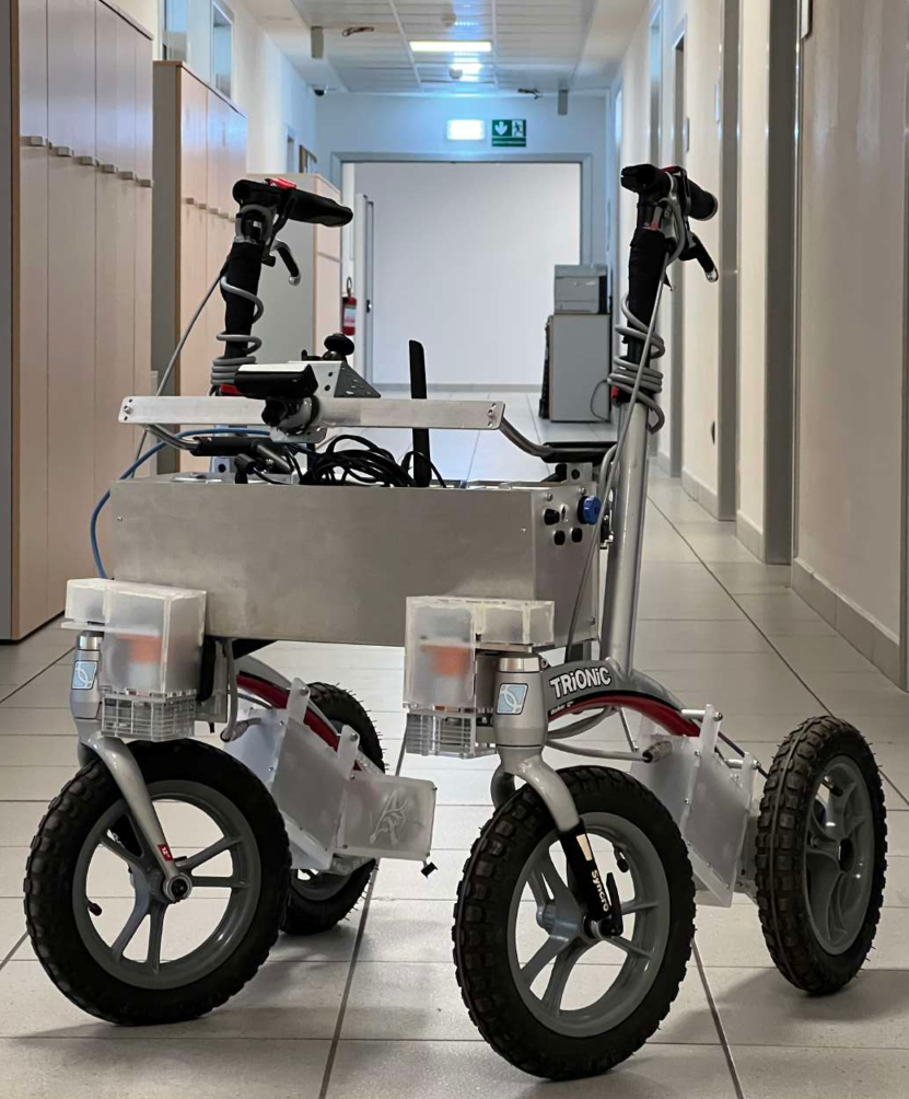
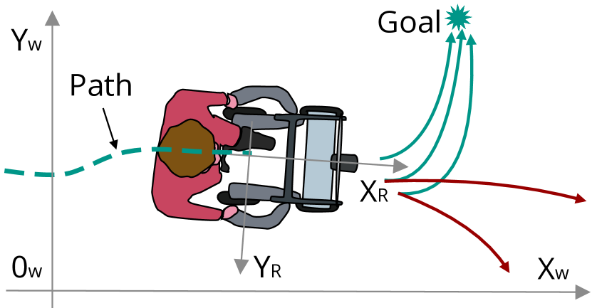
(a)	(b)

Figure 1: (a) The FriWalk used in our experiments. (b) Walker representation and adopted reference frames $\langle W\rangle$ and $\langle R\rangle$. In the example shown, the robot will allow any movement to the left (green curves), while it will perform a corrective action for all the non compliant ones (red curves).

In this paper we increase the level of our ambition: we aim to take away control from the human only in presence of erratic behaviours that deviate from what any other human would do in the same situation. At the same time, we aim to give the highest possible level of freedom to the user, without forcing her/him to follow a particular trajectory. This leads us to a central question: how do people move when they travel between two destinations in a known environment? The human body is extremely versatile and can generate innumerable motion patterns. However, in the past few years we learned that when humans walk, they tend to minimise the derivative of the curvature, which is a quantity related with the jerk [5]; this implies that they follow regular motion patterns similar to those generated by a nonholonomic vehicle. These trajectories are well approximated by clothoids (formal definition of a clothoid curve in Section 4.1). Still, different individuals generate different classes of trajectories. In terms of navigation, we can intuitively acknowledge that there are different ways to “turn right”, which are equally permissible and that together share the attribute of being a “right turn”. Starting from this observation, we have developed a learning-based framework to classify the features of human motion from synthetically generated trajectories, based on the geometric properties of the paths, thus creating a grid of expected behaviours. We define the minimalistic set {Left-turn, Right-turn, Straight} to identify the behaviour. Given a navigation task, we look for the behaviour that more closely matches the current motion in each portion of the traversed space. The motion control calculates the likelihood with which the current motion belongs to the current region of interest. When the likelihood becomes too low, it means that the human is behaving unexpectedly and the controller shifts the shared authority towards the robot. This way, the human is left in control as long as they perform as other people would do in the same environment. If the user is strongly committed to follow a path different from the one suggested by the system, s/he can force her way. When the system detects a strong opposition, it is disengaged for a configurable time unless a strong safety risk is detected (e.g., the presence of stairways).

From the implementation point of view, the walker is actuated with a visco–elastic control that regulates the steering angle. The classification confidence on the observed features is used as hyper-parameter to determine the visco–elastic force. The paradigm is illustrated in Fig. 1-b.

The paper is organised as follows. In Section 2, we summarise the most important literature contributions used as reference in this work. In Section 3 we formally describe the state of the problem, while in Section 4 our proposed framework is presented in detail. The simulation and experimental results on the robot are reported in Section 5, and finally in Section 6 we give our conclusions and announce future work directions.

2 Related work

This paper presents strong elements of novelty, which are supported by important previous research results in several areas that will be discussed in this section.

In this work we use a robotic walker which supports a person during locomotion. As described in [6] a robotic walker can have multiple functions to support different problems in the elderly locomotion. The robotic rollator can support the human’s mobility, increase safety and self-empowerment, compensate unbalanced gait, aid during the sitting or getting up phases and be used for rehabilitation [7] [8].

When robots need to move or to guide someone mimicking the human motion, it is essential to have a model of human motion. It is rather established that humans actually move following smooth trajectories [9] and that their motion model is well approximated by a unicycle [10], which naturally generates clothoid curves, also known as Euler spirals. As well as being used to express human-like motion [11], clothoids have important properties: they are smooth, have a linear curvature and can be expressed through a simple and analytic form that makes them easy to manage in real–time implementations [12]. Arechavaleta et al. [5] use a dynamic extension of the unicycle model and a numerical optimisation algorithm to find optimal solutions that well approximate the human locomotor trajectories. The cost functional minimises the time derivative of the curvature when the linear velocity is assumed to be constant and positive.

In our previous work [13] the human motion is successfully predicted using a neural network to learn the parameters of the Social Force Model, a physics-based model which describes the motion of people in social contexts, considering the person as a particle subject to attractive forces and repulsive forces. In works such as [14], [15] and [16] a combination of Inverse Reinforcement Learning (IRL) and the principle of maximum entropy was used to learn pedestrian decision making protocols from large volumes of data.

Different works investigated how to retrieve abstract information about the behaviour of humans from their trajectories, the majority of which use machine learning. For instance, Support Vector Machines (SVM) have been used to classify different walking styles and behaviours, including movements such as straight, left-turn, right-turn, U-turn, and not walking [17]. The input samples included the normalised coordinates, the orientation, the velocities, and the bounding boxes of the trajectories over the observation window. Instead, with Autoencoders (AEs), it is possible to reconstruct the data elaborated by the system while learning lower dimensional representations of the data, referred usually as its latent space representation. A combination of clustering and linear AEs was proposed by [18] to predict the future trajectory of vessels. The vessel state space is comprised of pose and linear velocities. In [19] a convolutional Variational Autoencoder (VAE) was used to train a latent representation of real-world vehicle trajectories, represented as a time series of 2D coordinates; the authors claim a reduction of the dimension of the latent space from 10 to 2, with evident benefits on the reconstruction ability without evident reduction of the classification accuracy. Although it is commonly believed that one of the goals of modern machine learning is to identify useful characteristics from simple time series of the coordinates, we argue that some prior geometrical information can be easily extracted and used as input for the neural model, in order to simplify its development and to improve the accuracy of the results. In a similar way, Lu et al. [20], augment the input of a Convolutional Autoencoder (CAE) with spatio-temporal information such as velocity, acceleration, and the heading change rate. As explained in [21], the encoder part of an autoencoder can be used to extract the features of the input and can be connected to a classification network to achieve classification abilities. This is exactly what we do in this work to classify the human trajectories. To the best of our knowledge there is no past work that uses the structure encoder + classification network to determine to which class the analysed trajectory pertains to (Left-turn, Right-turn, Straight).

As discussed below, we use an autoencoder network to extract the geometric parameters of each trajectory, and a second neural network to associate the geometric parameters with a class of behaviours. While the classification problem could be solved by other means, the use of learning approaches has two significant advantages: first, the use of NNs defines a general framework that can be easily generalised to other types of geometric features and behaviour classes; second, at runtime the classification produced by the NN can be used to produce a score that quantifies the degree of agreement between observed and expected behaviour. Specifically, during the control phase, we use a Bayesian technique to extract a measure of confidence on the behaviour currently followed by the human.

To the best of our knowledge, this paper is the first to use the neural network’s confidence score to control the amount of intervention in a path following task.

3 Problem Statement and Solution Overview

The reference model for the walker kinematic is the unicycle, described in discrete–time by the equations

$$\begin{cases}x(t_{k+1})=x(t_{k})+\cos(\theta(t_{k}))\delta_{t}v(t_{k}),\\ y(t_{k+1})=y(t_{k})+\sin(\theta(t_{k}))\delta_{t}v(t_{k}),\\ \theta(t_{k+1})=\theta(t_{k})+\delta_{t}\omega(t_{k}),\end{cases}$$ (1)

where $\bm{q}(t_{k})=\left[x(t_{k}),y(t_{k}),\theta(t_{k})\right]$ is the state of the vehicle, the coordinates $\left(x(t_{k}),y(t_{k})\right)$ identify the position of the mid point of the rear wheel inter-axle in the Cartesian plane $X_{w}\times Y_{w}$ expressed in the $\langle W\rangle=\left\{X_{w},Y_{w},Z_{w}\right\}$ world reference frame, $\theta(t_{k})$ is the longitudinal direction of the vehicle with respect to the $X_{w}$ axis, $v(t_{k})$ and $\omega(t_{k})$ are the longitudinal and angular velocities, respectively, and $\delta_{t}=t_{k+1}-t_{k}$ is the sampling time. For the particular problem at hand, $v(t_{k})$ is imposed by the human (also for safety reasons [22]), while $\omega(t_{k})$ is the control output and it is shared between the human and the robot. The problem to solve is to control the vehicle from a starting position $p_{0}=[x_{0},y_{0}]^{T}$ to a desired position $p_{f}$ in a known environment. The key requirement is to use the robot controller contribution to $\omega(t_{k})$ only when the human behaviour deviates significantly from the expected behaviour.

To this end, we need first to abstract the path following problem, that is usually defined in the space $\bm{q}(t_{k})$, into a high level representation that preserves the implicit features of the human trajectories. Therefore, let us denote by $\mathcal{H}\subset\mathbb{R}^{2}$ the path travelled by the human in $\langle W\rangle$, i.e., the sequence $\left(x(h_{k}),y(h_{k})\right)$ of coordinates expressed with respect to the curvilinear abscissa $h$ sampled at times $\delta_{t}$. Let $\mathcal{R}\subset\mathbb{R}^{2}$ be the reference path connecting $p_{0}$ to $p_{f}$. For both paths, we extract a set of features of dimensionality $m$, denoted as $\bm{z}_{k,\mathcal{H}}$, $\bm{z}_{k,\mathcal{R}}\in\mathbb{R}^{m}$, respectively, which are associated to a class of human-like behaviours {Left-turn, Right-turn, Straight}.

The overall framework of the proposed solution (sketched in Fig. 2) comprises the following steps:

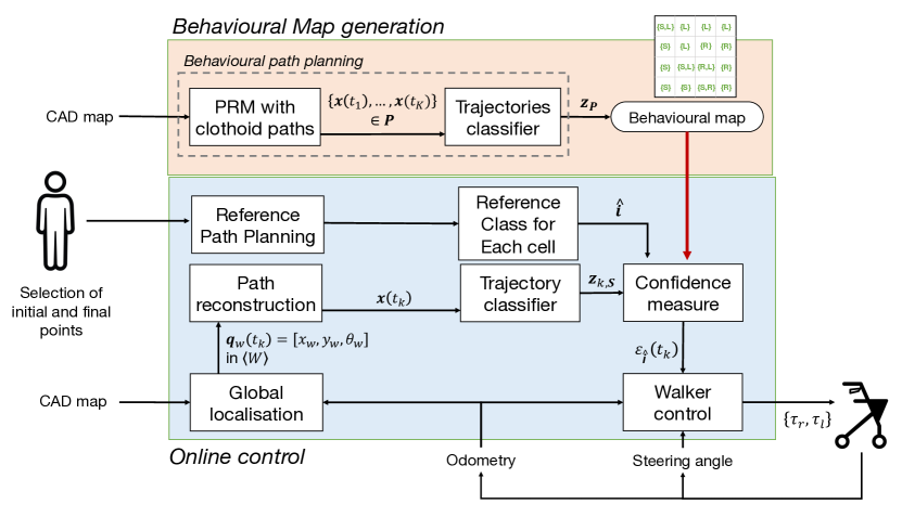
Figure 2: Overall scheme of the algorithm.

1. Given an a-priori map of the environment, composed of only the static obstacles information (walls, furniture…), we generate a large number of trajectories that are collision free and that mimic a human-like behaviour [23]. This operation is performed offline and is showed in Fig. 2 as the block: PRM with clothoid paths;

2. We partition the map using square cells. Then we classify the generated trajectories inside each cell into the {Left-turn, Right-turn, Straight} classes by using a neural network (Trajectories classifier block in Fig. 2). This classification is used to create a map of possible human-like manoeuvres that can be used to reach a specific location. This grid map will be called the behavioural map (Behavioural map block in Fig. 2).

3. Given the user initial position $p_{0}$, and a user–selected final position $p_{f}$ we connect them with a trajectory (the planning method will be explained later in the paper). This trajectory is characterised by its features $\bm{z}_{k,\mathcal{H}}$. For each portion of the ideal trajectory, we identify a reference cluster of trajectories generated at Step 1 and 2. From this cluster, we select a set of representative features $\bm{z}_{k,\mathcal{R}}$ (e.g., the centroid of the cluster). This allows us to compute the likelihood $\varepsilon(t_{k})$ (Confidence measure block in Fig. 2) and use it to generate the setting of the visco-elastic force used in our shared-authority control scheme (Walker control block in Fig. 2).

4 Model generation and behaviour–based control

The main pillars of our approach are an offline analysis of the environment that generates the behavioural map (i.e., the map of admissible behaviours for every area of the environment) and the online control module that adapts the shared authority controller to the degree of compliance of the user. The two modules are described next.

4.1 Behavioural map generation

Given the environment map, the behavioural map associates each area of the space with the class of trajectories (straight, right turn, left turn) possibly followed by humans when they behave “correctly”. This information is generated in different steps.

In the first step, we generate a Probabilistic Road Map (PRM) [24] covering the entire space. The PRM provides collision free geometric paths connecting any pair of locations in the space. The PRM is generated ensuring an average density of 4 nodes per squared meter, which is a good trade-off between fine distribution of nodes and elaboration time of the paths (e.g. in a 5x5 meters room we have an average of 100 nodes).

In the second step, we consider pairs of random starting positions and ending positions, find the shortest path connecting them through the PRM, and interpolate the different nodes by clothoids. A clothoid is a line with curvature proportional to the arc-length described by the equation $X(s)=x_{0}\!+\int_{0}^{s}\cos(\kappa^{\prime}\frac{\tau^{2}}{2}+\kappa_{0}\tau+\theta_{0})\textrm{d}\tau$, $Y(s)=y_{0}+\int_{0}^{s}\sin(\kappa^{\prime}\frac{\tau^{2}}{2}+\kappa_{0}\tau+\theta_{0})\textrm{d}\tau$, where $s$ is the curvilinear abscissa, $(x_{0},y_{0})$ is the Cartesian coordinate of the initial point, $\theta_{0}$ is the initial bearing, $\kappa_{0}$ is the initial curvature and $\kappa^{\prime}$ is the change rate of the curvature. The interpolation is done minimising the derivative of the squared curvature [12]. We can argue that the trajectories constructed in this way are a reasonable approximation of human-like trajectories, as supported by numerous results in the literature. The most important are in the work of Laumond et al. [23], in which clothoids are explicitly addressed as a good approximation of human trajectories, and in the work of Arechevaleta et al. [5], who have shown that humans tend to minimise the derivative of the squared curvature when they move.

In the third step, the environment is discretised in a grid map using 1x1 meters cells. For each trajectory $i$ intersecting a cell $j$, we identify a class $c_{i}^{(j)}$ in the finite set $\bm{c}$: $c_{i}^{(j)}\in\bm{c}$. For instance, one class could be “left turn” (L) or “move straight” (S). This operation is performed by the Trajectory Classifier, which allows us to partition each trajectory into a sequence of elementary moves (straight, left/right turn) and determine the class that identify each of them in every cell. To account for the different direction of motion of the $i$-th trajectory within the $j$-th cell, we associate the tangential direction $\theta_{i}^{(j)}$ , which is the mean direction of travel of the vehicle in the $j$-th cell w.r.t the map reference frame, with the class $c_{i}^{(j)}$. For instance if the user is moving with the walker straight from west to east the tangential direction $\theta_{i}^{(j)}$ will be 0. The set of all the pairs $\left(c_{i}^{(j)},\theta_{i}^{(j)}\right)$ form the behavioural map. In Figure 3 some of the synthetic trajectories are shown in magenta in a map of the Department of Engineering and Computer Science of the University of Trento, the grid map is shown in green and the corresponding sub-trajectories that will be fed to the classifier are highlighted with the blue circles. The starting points of the magenta trajectories are depicted with the red circles, while the ending points with the yellow circles.

Figure 3: Synthetic trajectories generated with PRM and clothoids.

The fundamental motion primitives forming the behaviour map are shown in light green in Figure 3.

The trajectory classifier. The trajectory features are extracted with an encoder neural network from the path geometry. More precisely, the $k$-th abscissa $s_{k}$ of the path $\mathcal{R}$, sampled such that $s_{k}-s_{k-1}=\delta_{s}$ is constant, is used to define the vector of geometric parameters

$$\bm{p}(s_{k})=\begin{bmatrix}x_{p}(s_{k})\\ y_{p}(s_{k})\\ \cos(\theta_{p}(s_{k}))\\ \sin(\theta_{p}(s_{k}))\\ \kappa_{p}(s_{k})\end{bmatrix},$$ (2)

where $x_{p}(s_{k})$ and $y_{p}(s_{k})$ are the Cartesian coordinates, while $\theta_{p}(s_{k})$ and $\kappa_{p}(s_{k})={d\theta_{p}(s_{k})}/{ds_{k}}$ are the tangential axis and the curvature of $\mathcal{R}$ in $\left(x_{p}(s_{k}),y_{p}(s_{k})\right)$, respectively. To account for the path characteristics, $n$ consecutive parameters are collected on the sampled abscissa coordinates $s_{k-(n-1)}$ to $s_{k}$, so as to build the matrix comprising $\bm{p}(s_{k-(n-1)})$ to $\bm{p}(s_{k})$, which is then normalised to avoid spatial biases, i.e.

$$\bm{x}_{p}(t_{k})=\begin{bmatrix}\left[x_{p}^{1},\dots,x_{p}^{n}\right]-x_{p}^{1}{\textbf{1}}^{T}\\ \left[y_{p}^{1},\dots,y_{p}^{n}\right]-y_{p}^{1}{\textbf{1}}^{T}\\ \cos(\theta_{p}^{1}),\dots,\cos(\theta_{p}^{n})\\ \sin(\theta_{p}^{1}),\dots,\sin(\theta_{p}^{n})\\ \kappa_{p}^{1},\dots,\kappa_{p}^{n}\end{bmatrix},$$ (3)

where 1 is an $1$-dimensional column vector with all ones, used for the normalisation of the position vectors, and we adopt the compact notation $x_{p}^{i}=x_{p}(s_{k-(n-i)})$. In order to avoid the problem of angular periodicity, we used both $\cos(\theta_{p}(s_{k-(n-i)}))$ and $\sin(\theta_{p}(s_{k-(n-i)}))$ instead of $\theta_{p}^{i}$.

In the training process of the encoder, $\bm{x}_{p}(t_{k})\in\mathbb{R}^{5\times n}$ is used as input. The weights of the encoder are learned by training an autoencoder and minimising the reconstruction error between $\bm{x}_{p}(s_{k})$ and the reconstructed output $\tilde{\bm{x}}_{p}(s_{k})$. The encoder and the decoder sub-networks of the autoencoder, have a symmetrical structure: the input $\bm{x}_{p}(t_{k})$ passes through $3$ convolutions and $3$ fully-connected layers, resulting in a final latent space of $m=5$ neurons. The decoder, then, has the same structure, but takes as input the latent space $\bm{z}_{k,\mathcal{R}}\in\mathbb{R}^{5}$.

After learning the autoencoder weights, the decoder sub-network is discarded as we will use the latent space of the autoencoder as a compressed representation of the human behaviour (Net1). A second neural network (Net2) classifies $\bm{z}_{k,\mathcal{R}}$ into the behavioural classes in the set $\bm{c}$. More precisely, the behaviour is identified in the minimalistic set {Left-turn, Right-turn, Straight} and encoded by the numeric label $\bm{c}=\left\{1,2,3\right\}$. Hence, during the learning phase we define the transformation

$$\tilde{\bm{c}}=h_{\psi}\left(\bm{z}_{k,\mathcal{R}}\right),$$ (4)

where $\psi$ is a set of parameters obtained by minimising the cross–entropy between the predicted $\tilde{\bm{c}}$ and the actual $\bm{c}$ class. In the architecture of the classifier network the input latent feature $\bm{z}_{k,\mathcal{R}}$ of $5$ neurons passes through a single fully-connected layer with just $3$ neurons. Therefore, the combination of the neural networks maps the geometric characteristics of the path $\bm{x}_{p}(s_{k})$ into the trajectory classes encoded in $\bm{c}$. As a final step, a $\operatorname{softmax}(\cdot)$ activation function is applied to the three output neurons of Net2 to retrieve the confidence $\varepsilon_{i}(s_{k})$ (or equivalently $\varepsilon_{i}(t_{k})$) of the class $c_{i}\in\bm{c}$, i.e. $\sum_{i=1}^{3}\varepsilon_{i}(s_{k})=1$. Notice that this same network is adopted to classify the synthetic generated paths and the current user behaviour, as will be explained in the next Section 4.2.

Geometry of the Grid

In the discussion above we suggest a decomposition into a grid made of square cells. This choice is not mandatory. For other types of environments with the presence of static obstacles with non-rectangular shape, it could be more convenient to use a different type of cell decomposition (e.g., maximum clearance maps, maps resulting from plane sweep, etc.) [25]. The technique proposed in the paper would not be significantly affected by the choices of a different polygonal geometry.

4.2 Online Control

As a first step in the online control, the user selects their destination ($p_{f}$) starting from the initial point $p_{0}$ where the device is currently located. It is prudent to impose limits on the maximum traveled distance when dealing with individuals who may have limited mobility or other frailties. Equally important is the optimisation of routes connecting subgoals based on specific metrics. We’ve previously tackled these challenges and provided solutions in our earlier work [26]. In our current research, we assume that all pertinent decisions regarding these constraints and optimisation criteria have been predetermined before executing our algorithm.

Following the same steps as for the behaviour map generation, the system connects the two points via the PRM and interpolates the intermediate points by using a G2 spline that minimises the derivative of the squared curvature. This allows us to determine for the current cell $j$ the reference class and its orientation $(c^{(j)}_{\hat{i}},\theta^{(j)}_{\hat{i}})$. Roughly speaking, this pair encodes the most sensible behaviour that a human would follow if they want to reach $p_{f}$ from the cell $j$, and will be used to measure the degree of compliance of the human.

A custom path reconstruction module, described in [11], processes the odometry information received by the FriWalk and produces in real–time $\mathcal{H}$ and, hence, the sets $\bm{x}_{s}(s_{k})$. The currently performed path $\bm{x}_{s}(s_{k})$ is reduced to its features $\bm{z}_{k,\mathcal{H}}$ using the neural network explained in the previous Section 4.1. These features are compared to the ones stored in the Behavioural map to obtain the confidence value $\varepsilon_{\hat{i}}(s_{k})$ (Confidence measure in Figure 2). A high confidence means that the features of the user motion are compatible to a large extent with the class $c^{(j)}_{\hat{i}}$, while a low confidence means that the user is drifting away from the expected behaviour. Hence, $\varepsilon_{\hat{i}}(s_{k})$ will be used as a hyper-parameter in the control of the Walker.

The control module is designed synthesising a visco–elastic torque that is applied to the steering angle of the front wheels of the robot. The idea of the visco-elastic control [27] can be described as follows. Suppose that the path synthesised by the system (desired trajectory) is described by means of the desired steering angle $\theta^{\star}$ and steering velocity $\dot{\theta}$. Let $\theta$ and $\dot{\theta}$ be the actual measured or estimated values. The torque applied to the system is given by

$$\tau=-a\left(\theta-\theta^{\star}\right)-b\left(\dot{\theta}-\dot{\theta}^{\star}\right).$$

In simple words, the vehicle is governed by a torque generated by a spring-damper system. Importantly, the spring constant $a$ and the damper constant $b$ are not time invariant but are functions. In our original idea [27] these functions depend on the deviation from the desired path: the larger the deviation from the desired path the stiffer become the controller. This controller is practically stable, meaning that it secures the convergence of the error to a neighbourhood of the origin.

To this end, we first define the actual right (left) wheel angle as $\alpha_{r}$ ($\alpha_{l}$), which can be measured by an absolute encoder (we dropped the reference to the time $t_{k}$ for ease of notation). The states are expressed in the robot reference frame $\langle R\rangle=\left\{X_{r},Y_{r},Z_{r}\right\}$, with $X_{R}$ oriented along the longitudinal direction and $Z_{R}$ pointing upwards. The desired wheel angles $\alpha_{r}^{\star}$ and $\alpha_{l}^{\star}$, instead, can be obtained by the desired angular velocity $\omega^{\star}$ (computed using the behaviour map associated with the desired class $(c^{(j)}_{\hat{i}},\theta^{(j)}_{\hat{i}})$), the actual longitudinal velocity $v$ (obtained by the encoders on the rear wheels) and the Ackermann steering geometry. Hence, the wheels orientation errors

$$e_{\alpha_{r}}=\alpha_{r}^{\star}-\alpha_{r}\mbox{ and }e_{\alpha_{l}}=\alpha_{l}^{\star}-\alpha_{l},$$

can be immediately obtained. The visco-elastic controller that controls the torque to apply to the wheel is determined as

$$\tau_{\alpha_{r}}=ae_{\alpha_{r}}+b\dot{e}_{\alpha_{r}},$$ (5)

and the same for the left wheel to obtain $\tau_{\alpha_{l}}$.

While this controller accounts for the local direction that the vehicle has to take w.r.t. $\langle R\rangle$ (i.e., the curvature of the path), we also compute the absolute orientation error of the front wheels in $\langle W\rangle$. Again, using the desired orientation $\theta_{\hat{i}}^{(j)}$, and thus compute the desired wheel direction $\beta_{r}$ in $\langle W\rangle$ as

$$e_{\beta_{r}}=(\theta^{\star}+\alpha_{r}^{\star})-(\theta+\alpha_{r}).$$

The same can be applied to $\beta_{l}$. Hence, we can compute the same visco-elastic controller in (5) for the errors $\beta_{r}$ and $\beta_{l}$ (with the same parameters $a$ and $b$), thus obtaining the final control laws

$$\tau_{r}=\lambda\tau_{\alpha_{r}}+\tau_{\beta_{r}}\mbox{ and }\tau_{l}=\lambda\tau_{\alpha_{l}}+\tau_{\beta_{l}}.$$ (6)

The parameters $\lambda$, $a$ and $b$ are functions of the confidence $\varepsilon_{\hat{i}}(t_{k})$ associated with the reference class $c_{\hat{i}}^{(j)}$ by means of

$$\lambda=1-\varepsilon_{\hat{i}}(t_{k}),$$ (7)

$$a=a_{0}+a_{1}\lambda,$$

$$b=b_{0}+b_{1}\lambda.$$

The $a$ parameters influence the elasticity of the control law, while the $b$ parameters influence its viscosity. Specifically, $a_{0}$ and $b_{0}$ are the minimum coefficients used when the controller does not intervene (when the confidence is high). The $a_{1}$ and $b_{1}$ are modulated by the hyperparameter epsilon (the confidence). This means that increasing values of higher $a_{0}$ and $b_{0}$ will result in more intervention from the control, even when the human is performing correct movements. Similarly, the values of $a_{1}$ and $b_{1}$ widen or shrink the range of the applied control signal between when the system intervenes and when it does not. These parameters have to be fine-tuned by trail-and-error sessions on the specific application.

To summarise, we first compute the reference class $c^{(j)}_{\hat{i}}$, then from the actual state $\bm{x}_{s}(t_{k})$ we compute $\varepsilon_{\hat{i}}(t_{k})$ and then, by means of (7), the desired torques are computed with (6). The term $b_{0}$ is needed to avoid oscillatory behaviours while $a_{0}$ is needed to generate the correct control signal that forces the wheel angle $\alpha_{r}$ ($\alpha_{l}$) to the desired value. In this way, when the confidence is high (i.e., $\lambda$ is low), the applied torque is predominantly imposed by the user and the computed torques $\tau_{r}$ and $\tau_{l}$ tend to zero. The system, instead, becomes increasingly authoritative (i.e., torques $\tau_{r}$ and $\tau_{l}$ imposed by the system) when $\lambda$ gets closer to $1$.

Management of obstacles and of exceptions

The approach outlined above hinges on the definition of a reference trajectory for each cell (given by the centroid of the most probable cluster) and on the application of visco-elastic control to make sure that the user does not deviate too much. Two type of exceptions can occur:

1. An unexpected dynamic obstacle (e.g., another human) materialises,

2. The user strongly opposes the suggestion and forces her/his way.

The first case is handled by using the so called reactive planning [28]: the system replans a new clothoidal trajectory that travels around the obstacle and joins into the reference trajectory as soon as the obstacle is overcome. This change has no significant impact on the framework: we can either use the visco-elastic control modulated by the likelihood $\epsilon$ or opt for a stiffer behaviour until the anomaly is over. For the second exception, we interpret the strong opposition of the user as her/his better understanding of the scenario. Therefore, we disengage the guidance system for a reconfigurable time. This choice does not apply if the user is travelling across areas that we deem dangerous (e.g., a stairway).

5 Experimental Validation and Results

Generation of the behavioural map. The experimental validation of the approach has been carried out in our Department premises. The first step of the approach was the construction of the behaviour map generating the described human-like synthetic trajectories (some examples are shown in Figure 3). For the training of Net1 and Net2 we focused on an area consisting of two intersecting corridors (conventional cross–intersection). We simulated $1800$ paths selecting randomly pairs of waypoint positions $p_{0}$ and $p_{f}$. The simulations were equally partitioned in the Left-turn, Right-turn and Straight classes. We select $n=12$ samples for the inputs $\bf{x}$ , as shown in Eq. (3), this implies that the encoder will have 60 input features. A step size of $\delta_{s}=0.1$ m has been chosen to sample the trajectory. A fraction of $80\%$ of the dataset was used as training set, while the remaining samples were randomly selected for the validation. Both Net1 and Net2 were implemented in Keras and trained with the Adam optimiser with a learning rate of $0.001$, batch size $64$, and number of epochs $300$ using a 2.7 GHz Intel Core i7 processor. Net1 was trained using the set of $\bf{x}$ as both inputs and outputs of the network. Then, we transferred the learned weights of the encoder in the Net2, and performed a supervised training by comparing its estimates with the one-hot encoded labels of classes {Left-turn, Right-turn, Straight}.

In Table 1, we report the inference accuracy of the network Net1 on the validation set, in terms of Root Mean Squared Error (RMSE).

Table 1: RMSE of the Net1 and the precision discovery rate of the Net2 on the validation set of the synthetic trajectories.

	$x$ (m)	$y$ (m)	$\cos(\theta)$	$\sin(\theta)$	$\kappa$
RMSE	0.0076	0.0118	0.0293	0.0449	0.0241
	Left	Right	Straight	Average
Accuracy	88.4$\%$	88.3$\%$	76.8$\%$	84.3$\%$

The results show that the network was correctly trained on the dataset, and the even distribution of the error over the different components of the input indicates that no bias was produced in favour of a particular component. The parameters $a$ and $b$, as explained in Section 4.2, are functions of the confidence of the manoeuvre. For the angular velocity $\omega$, the parameters of the visco-elastic controller in (7) were set to $a_{0}=25$ N, $a_{1}=15$ N, $b_{0}=15$ Ns and $b_{1}=10$ Ns. For the steering wheel direction $\beta$, the parameters of the visco-elastic controller were set to $a_{0}=25$ N, $b_{0}=25$ Ns. These parameters were set leveraging our experience with the system. Changing such parameters, modifies the amount of intervention of the robot control.

The validation results for the training of the network Net2 are reported in Table 1, showing the accuracy of the inferred classes. It can be noticed that the Left and Right classes obtained a higher percentage with respect to the Straight class: the reason behind this behaviour is that the trajectories of the Straight class include features in common with the ones of the other classes (e.g., when the human slightly bends along an almost straight path). This is noticeable in Figure 3, where the sub-trajectories not always are distinguishable between turns and straight sectors.

5.1 Experiments with the FriWalk

The experimental evaluation of the approach presented in Section 3 and Section 4 was conducted on the real FriWalk in an indoor hallway at the University of Trento. The vehicle is endowed with front electric DC motors to control the angle of the front wheels. The localisation system of the robot comprises incremental encoders in the rear wheels and absolute encoders for the front wheels, used in combination with a 2D camera system. A collection of ArUco markers was placed in the testing area, which has a dimension of roughly $7\times 7$ m, allowing the walker to localise itself with sufficient accuracy (error below $20$ cm, as reported in [29]). A ROS interface was used to send the control to the actuators and to receive the localisation data, including the odometry-based estimates of $\bm{q}(t_{k})$ in $\langle W\rangle$ and the angular position of the wheels $\alpha_{r}$ and $\alpha_{l}$ in $\langle R\rangle$. We fixed the initial and final waypoint areas for the tests and we executed offline the behavioural path planning described in Section 4.1, obtaining the mentioned behavioural map. We then executed several trials of the same mission, varying the general behaviour of the human experimenter between three macro categories: following diligently the predefined mission, following the mission roughly and deviating from the mission. Figure 5-a shows the control action of the robot while the human moved for the leftmost corridor towards an exit on the upper part of the map (see Figure 4-b).

(a)
(b)

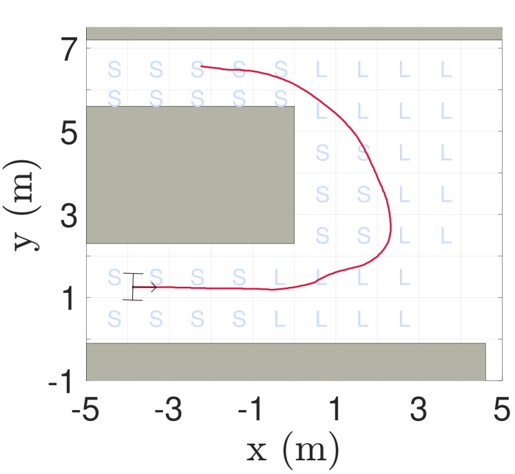
Figure 4: (a) Photo of the experimental area and (b) the associated behavioural map.

(a)
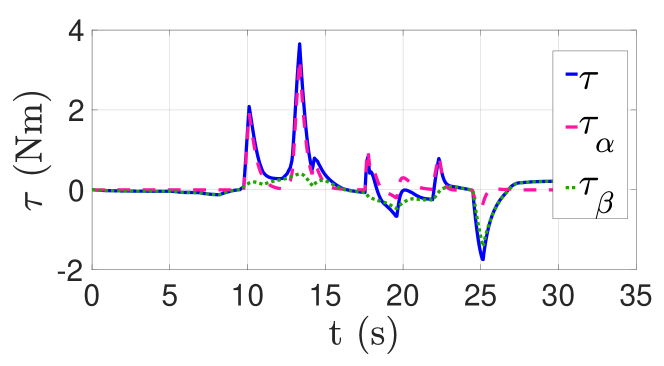
(b)

Figure 5: (a) Torque controls for $e_{\alpha_{r}}$ and $e_{\alpha_{l}}$ (magenta-dashed line) and for $e_{\beta_{r}}$ and $e_{\beta_{l}}$ (green-dotted line) applied to the walker front wheels while performing the trajectory in (Fig 4-b). (b) confidence for Left-turn (grey-solid line), Right-turn (purple-dashed line) and Straight (yellow-dotted line).

After $10$ seconds from the beginning of the experiment, the user kept walking straight an area where the Left-turn class was instead foreseen: the low likelihood on the Left behaviour (grey line in Figure 5-b) triggered a compensating action on the control signal $\tau_{\alpha_{r}}$ and $\tau_{\alpha_{l}}$ in (6) (dashed magenta curve in Figure 5-a), thus causing a compensation in the trajectory. This intervention results into the increasing likelihood of the Left-turn behaviour class (grey line in Figure 5-b). Similarly, as the human tried to steer right after $13$ seconds, the corresponding Right-turn behaviour was caught (purple dashed line in Fig. 5-b) and the authority was again transferred to the robot, i.e., the human was progressively pushed towards the correct turning behaviour. Notice that when the compensation action occurs, the human user corrects the erratic behaviour in a few instants, indulging the robot action and indirectly lowering the control action. Hence, the robot action is perceived as a brief suggestion that vanishes immediately if the user follows the change of the route, otherwise the control action will persistently assist the manoeuvre towards the correct direction.

In Figure 6, we depict the performance of the control for three different user’s behaviours.

(a)
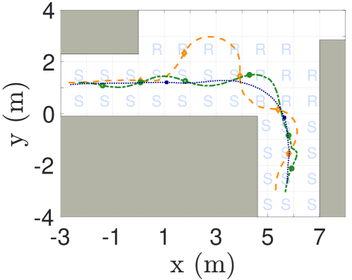
(b)

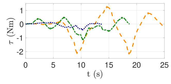
Figure 6: Experimental evidence of the control action behaviour in case of a user acting purposely against the desired path (orange lines), making slight deviations (green lines) or adhere to the planned path (blue lines). The resulting path (a) and the relative control actions (b) are reported.

When the person is compliant with the planning (blue trajectory), the control does not intervene, so the person is fully in charge and do not feel any opposing action from the robot. When, instead, the user purposely acts against the planned path, the control actions are extremely evident (orange trajectory). Finally, in the most typical case, the control acts loosely without excessively forcing the path correction (green trajectory), keeping the motion in the appropriate direction (please also refer to the multimedia complementary material accompanying this paper for further examples).

5.2 User evaluation

Since this work hinges for a large part on human-robot interaction, a qualitative evaluation of the system behaviour was needed to validate the user acceptability. Simple experiments were defined to propose the control strategy to participants, which were followed by a brief poll to evaluate the level of appreciation of the person. All the participants were informed that data collection and the information provided are covered by the ethical rules of the Research Ethics Committee, which approved this experiment, and that they could quit the experiment at anytime. Once consent was obtained they were invited to perform the tasks with the FriWalk. The experiment was performed by 16 adults in the age range of 21-50 years old, without motor nor cognitive impairments. The participants were 11 males and 5 females, all from the University of Trento. The participants do not use walking aid devices in their daily lives.

The experiments were held in a single experimental session for each participant with a maximum duration of $15$ minutes, divided into three main parts. The participant tried the walker with two navigation techniques: the solution here presented and a visco–elastic control applied to force the vehicle on an optimally planned path [27] used as comparison. Both navigation techniques were applied to the same indoor environment, with the same points of departure and arrival and both had similar performance and efficiency in terms of data requirements, computing power, and scalability. Moreover, the order of presentation of the two techniques was randomised to obtain comparable results from the polls, and to the participants they were presented as navigation technique A and navigation technique B. The participant would not initially be told which of the two navigation techniques is the result of this study so as to avoid influencing the perceptions of the driving experience. The participants were asked to walk naturally with the aid of the walker from their current initial position to a specific point showed to them. They were asked to move compliantly to the target and then a in a second attempt to move erratically to the target or even go to the wrong direction. Finally, the participant was asked to answer a short questionnaire in which a qualitative evaluation of the aspects of the two navigation methods tried, and a final question were asked, in which these methods were compared. The participant could decide to repeat the navigation tests several times before the polls if it was necessary to achieve a better understanding of its functioning, but none of them asked to repeat the test. The participant could move freely in the environment, keeping in mind that the navigation techniques under test have no mechanism to avoid obstacles. It was the participant who took charge of avoiding hitting the walls and any other obstacles that may arise during the experiment.

In Table 2 and Table 3 are reported the poll results.

Table 2: User evaluation (yes)

Question	Visco–elastic control	Behavioural maps control
Was it evident that was the walker to decide the path to follow?	$87.5\%$	$12.5\%$
Have you felt to be pulled, pushed or stuck?	$37.5\%$	$12.5\%$

Table 3: User evaluation (mean - standard deviation)

Question	Visco–elastic control	Behavioural maps control
The experience with the walker was pleasant?	$3.38$ - $0.92$	$4.75$ - $0.46$
You had the impression you had no control?	$2.88$ - $0.83$	$1.38$ - $0.74$
The walker hindered/prevented your usual way of walking?	$1.63$ - $0.74$	$1.00$ - $0.00$

The questions in Table 2 could be answered with ”yes” or ”no”. In the table, beside its relative question, there is the percentage of answers that were ”yes”. The questions of Table 3 could be answered with a value between 1 and 5, were 1 means ”not at all” and 5 means ”extremely”. The aggregate result is presented as mean and standard deviation of the answers.

From the results in Table 2 we can deduct that the Behavioural Maps’ control is less intrusive, aiding the user’s navigation without sacrificing her/his comfort. Through the questions reported in Table 3, we could evaluate the cognitive aspects derived from the experience of using the walker. We can observe a good level of accordance between the $12.5\%$ reported in both questions of Table 2 for the Behavioural map control and $1.38$ reported in the second question of Table 3. Likewise, the low performance reported for the visco-elastic control in the first question of Table 3 is an evident consequence of its perceived level of authority and intrusiveness reported in Table 2. The evident conclusion is that the impression of being in control (at least in part) has an evident positive impact on the quality of the user’s experience.

Moreover $100\%$ of the participants preferred the control strategy proposed in this paper over the classic visco–elastic control. Some of the motivations were that our method gives more autonomy and freedom to perform any path while the turns were performed more softly, without forcing the participant to a particular trajectory.

In this section, we have shown a complete experimental evaluation both from the perspective of the quantitative performance and of the user experience. In both cases, the results are very good and prove that this framework provide a navigation assistance, which guarantees a good level of agreement of the user trajectories with socially acceptable behaviours limiting at the same time the level of interference of the system with the user’s choices.

6 Conclusions

In this paper, we have considered a robot-assisted navigation scenario. We adopted a shared authority controller, in which the navigation decisions are shared between the human and the robot. The key contribution of the paper is to show how this decision can be taken based on the degree of conformance of the human’s behaviour with the standard behaviour taken by humans in similar situation. We substantiated this idea by a combination of learning and control approaches, where the former are used to understand and classify the human behaviours and the latter to change the visco-elastic parameters of the guidance algorithm to adapt to the level of confidence that we have on the human behaviour.

In the future, we will continue this research in many directions. The most important one is removing the need for a prior knowledge of the map. A possible approach could be to study behavioural templates associated with specific features of the environment. During the execution, the system could classify the environment features and associate them on-the-fly with the expected behavioural templates. We will also investigate other methods to increase the accuracy in distinguishing between turns and going straight. This could be done increasing the number of features or increasing the number of classes. The assumption that humans use clothoids as their preferred choice is certainly true in the majority of the cases and, especially, when the road in front of the human is sufficiently clear. In case these conditions are not met (e.g., a densely populated environment), the assumption could no longer hold. In the future we plan to analyse also these special cases. In addition, it is possible that people deviate from this standard motion pattern because of cognitive or physical problems. In some of theses cases, using a clothoid as a reference trajectory could be seen as a rehabilitation policy. These hypotheses needs further investigations. At last we want to evaluate what happens when the goal is changed dynamically during the online execution. This should not cause any abnormal behaviour in the control system: if the goal is altered while the user is in motion, the current motion may no longer align with the desired one. Consequently, the probability score for the desired motion class may decrease, leading to a change in the control hyperparameter. This adjustment increases the amount of control interventions, resulting in a more substantial elastic recall and a smoother correction of the current motion.

References

- \bibcommenthead
- [1] F.O. Flemisch, C.A. Adams, S.R. Conway, K.H. Goodrich, M.T. Palmer, P.C. Schutte, The h-metaphor as a guideline for vehicle automation and interaction. Tech. rep., RWTH Aachen University (2003)
- [2] M. Andreetto, S. Divan, D. Fontanelli, L. Palopoli, Path following with authority sharing between humans and passive robotic walkers equipped with low-cost actuators. IEEE Robotics and Automation Letters 2(4), 2271–2278 (2017)
- [3] V. Magnago, M. Andreetto, S. Divan, D. Fontanelli, L. Palopoli, Ruling the Control Authority of a Service Robot based on Information Precision. Proc. IEEE International Conference on Robotics and Automation (ICRA) pp. 7204–7210 (2018). 10.1109/ICRA.2018.8460714
- [4] P. Bevilacqua, M. Frego, E. Bertolazzi, D. Fontanelli, L. Palopoli, F. Biral, Path planning maximising human comfort for assistive robots. 2016 IEEE Conference on Control Applications (CCA) pp. 1421–1427 (2016). 10.1109/CCA.2016.7588006
- [5] G. Arechavaleta, J.P. Laumond, H. Hicheur, A. Berthoz, An optimality principle governing human walking. IEEE Transactions on Robotics 24(1), 5–14 (2008). 10.1109/TRO.2008.915449
- [6] G. Bieber, W. Chodan, R. Bader, B. Hölle, P. Herrmann, I. Dreher, Roro: A new robotic rollator concept to assist the elderly and caregivers. Proceedings of the 12th ACM International Conference on Pervasive Technologies Related to Assistive Environments p. 430–434 (2019). 10.1145/3316782.3322779
- [7] L. Palopoli, A. Argyros, J. Birchbauer, A. Colombo, D. Fontanelli, A. Legay, A. Garulli, A. Giannitrapani, D. Macii, F. Moro, P. Nazemzadeh, P. Panteleris, R. Passerone, G. Poier, D. Prattichizzo, T. Rizano, L. Rizzon, S. Scheggi, S. Sedwards, Navigation assistance and guidance of older adults across complex public spaces: the dali approach. Intelligent Service Robotics 8, 77–92 (2015). 10.1007/s11370-015-0169-y
- [8] A. Lopes, J. Rodrigues, J. Perdigao, G. Pires, U. Nunes, A new hybrid motion planner: Applied in a brain-actuated robotic wheelchair. IEEE Robotics & Automation Magazine 23(4), 82–93 (2016). 10.1109/MRA.2016.2605403
- [9] G. Arechavaleta, J.P. Laumond, H. Hicheur, A. Berthoz, On the nonholonomic nature of human locomotion. Autonomous Robots 25(1), 25–35 (2008)
- [10] F. Farina, D. Fontanelli, A. Garulli, A. Giannitrapani, D. Prattichizzo, Walking ahead: The headed social force model. PloS one 12(1), e0169734 (2017)
- [11] A. Antonucci, P. Bevilacqua, S. Leonardi, L. Palopoli, D. Fontanelli, Humans as path-finders for safe navigation. arXiv preprint arXiv:2107.03079 (2021)
- [12] E. Bertolazzi, M. Frego, On the g2 hermite interpolation problem with clothoids. Journal of Computational and Applied Mathematics 341, 99–116 (2018)
- [13] A. Antonucci, G.R. Papini, P. Bevilacqua, L. Palopoli, D. Fontanelli, Efficient Prediction of Human Motion for Real-Time Robotics Applications with Physics-inspired Neural Networks. IEEE Access 10, 144–157 (2021). 10.1109/ACCESS.2021.3138614
- [14] B.D. Ziebart, N. Ratliff, G. Gallagher, C. Mertz, K. Peterson, J.A. Bagnell, M. Hebert, A.K. Dey, S. Srinivasa, Planning-based prediction for pedestrians. 2009 IEEE/RSJ International Conference on Intelligent Robots and Systems pp. 3931–3936 (2009). 10.1109/IROS.2009.5354147
- [15] M. Kuderer, H. Kretzschmar, C. Sprunk, W. Burgard, Feature-based prediction of trajectories for socially compliant navigation. Robotics: Science and Systems VIII pp. 193–200 (2013)
- [16] H. Kretzschmar, M. Spies, C. Sprunk, W. Burgard, Socially compliant mobile robot navigation via inverse reinforcement learning. The International Journal of Robotics Research 35(11), 1289–1307 (2016). 10.1177/0278364915619772
- [17] T. Kanda, D.F. Glas, M. Shiomi, N. Hagita, Abstracting people’s trajectories for social robots to proactively approach customers. IEEE Transactions on Robotics 25(6), 1382–1396 (2009)
- [18] B. Murray, L.P. Perera, A dual linear autoencoder approach for vessel trajectory prediction using historical ais data. Ocean Engineering 209, 107478 (2020)
- [19] O. Rákos, S. Aradi, T. Bécsi, Z. Szalay, Compression of vehicle trajectories with a variational autoencoder. Applied Sciences 10(19), 6739 (2020)
- [20] S. Lu, Y. Xia, Dual supervised autoencoder based trajectory classification using enhanced spatio-temporal information. IEEE Access 8, 173918–173932 (2020)
- [21] D. Bank, N. Koenigstein, R. Giryes, Autoencoders. Machine Learning for Data Science Handbook: Data Mining and Knowledge Discovery Handbook pp. 353–374 (2023)
- [22] M. Andreetto, S. Divan, F. Ferrari, D. Fontanelli, L. Palopoli, F. Zenatti, Simulating passivity for Robotic Walkers via Authority-Sharing. IEEE Robotics and Automation Letters 3(2), 1306–1313 (2018). 10.1109/LRA.2018.2797321
- [23] J.P. Laumond, G. Arechavaleta, T.V.A. Truong, H. Hicheur, Q.C. Pham, A. Berthoz, A. Berthoz, The words of the human locomotion. ISRR (2010). 10.1007/978-3-642-14743-2_4
- [24] L. Kavraki, P. Svestka, J.C. Latombe, M. Overmars, Probabilistic roadmaps for path planning in high-dimensional configuration spaces. IEEE Transactions on Robotics and Automation 12(4), 566–580 (1996). 10.1109/70.508439
- [25] S.M. LaValle, Planning algorithms (Cambridge university press, 2006)
- [26] P. Bevilacqua, M. Frego, L. Palopoli, D. Fontanelli, Activity planning for assistive robots using chance-constrained stochastic programming. IEEE Transactions on Industrial Informatics 17(6), 3950–3961 (2020)
- [27] M. Andreetto, et al., Authority-sharing control of assistive robotic walkers. PhD Thesis (2019)
- [28] P. Bevilacqua, M. Frego, D. Fontanelli, L. Palopoli, Reactive Planning for Assistive Robots. IEEE Robotics and Automation Letters 3(2), 1276–1283 (2018). 10.1109/LRA.2018.2795642
- [29] P. Nazemzadeh, D. Fontanelli, D. Macii, L. Palopoli, Indoor Localization of Mobile Robots through QR Code Detection and Dead Reckoning Data Fusion. IEEE/ASME Transactions on Mechatronics 22(6), 2588–2599 (2017). 10.1109/TMECH.2017.2762598