Search for Non-Tensorial Gravitational-Wave Backgrounds in the NANOGrav
15-Year Data Set

Abstract

The recent detection of a stochastic signal in the NANOGrav 15-year data set has aroused great interest in uncovering its origin. However, the evidence for the Hellings-Downs correlations, a key signature of the gravitational-wave background (GWB) predicted by general relativity, remains inconclusive. In this letter, we search for an isotropic non-tensorial GWB, allowed by general metric theories of gravity, in the NANOGrav 15-year data set. Our analysis reveals a Bayes factor of approximately 2.5, comparing the quadrupolar (tensor transverse, TT) correlations to the scalar transverse (ST) correlations, suggesting that the ST correlations provide a comparable explanation for the observed stochastic signal in the NANOGrav data. We obtain the median and the $90\%$ equal-tail amplitudes as $\mathcal{A}_{\mathrm{ST}}=7.8^{+5.1}_{-3.5}\times 10^{-15}$ at the frequency of 1/year. Furthermore, we find that the vector longitudinal (VL) and scalar longitudinal (SL) correlations are weakly and strongly disfavoured by data, respectively, yielding upper limits on the amplitudes: $\mathcal{A}_{\mathrm{VL}}^{95\%}\lesssim 1.7\times 10^{-15}$ and $\mathcal{A}_{\mathrm{SL}}^{95\%}\lesssim 7.4\times 10^{-17}$. Lastly, we fit the NANOGrav data with the general transverse (GT) correlations parameterized by a free parameter $\alpha$. Our analysis yields $\alpha=1.74^{+1.18}_{-1.41}$, thus excluding both the TT ($\alpha=3$) and ST ($\alpha=0$) models at the $90\%$ confidence level.

Introduction. A pulsar timing array (PTA) is dedicated to the detection of gravitational waves (GWs) with frequencies in the nanohertz range by regularly monitoring the spatially correlated fluctuations caused by GWs on the time of arrivals (TOAs) of radio pulses emitted by an array of pulsars Sazhin (1978); Detweiler (1979); Foster and Backer (1990). There are three major PTA projects: the European PTA (EPTA) Kramer and Champion (2013), the North American Nanoherz Observatory for GWs (NANOGrav) McLaughlin (2013), and the Parkes PTA (PPTA) Manchester et al. (2013). Over the course of more than a decade, these projects have been monitoring the TOAs from dozens of millisecond pulsars with an observation cadence ranging from weekly to monthly. These PTAs along with the Indian PTA (InPTA) Joshi et al. (2018) constitute the International PTA (IPTA) Hobbs et al. (2010); Manchester (2013). Meanwhile, the Chinese PTA (CPTA) Lee (2016) and the MeerKAT PTA (MPTA) Miles et al. (2023) hold observer status within the IPTA.

Recently, NANOGrav Agazie et al. (2023a, b), EPTA+InPTA Antoniadis et al. (2023a, b), PPTA Zic et al. (2023); Reardon et al. (2023), and CPTA Xu et al. (2023) have independently announced compelling evidence for a stochastic signal in their latest data sets. These data sets demonstrate varying levels of significance in supporting the presence of Hellings-Downs (HD) Hellings and Downs (1983) spatial correlations as predicted by general relativity. While the PTA window covers a broad range of possible sources Li et al. (2019); Vagnozzi (2021); Chen et al. (2021); Wu et al. (2022a); Chen et al. (2022a); Benetti et al. (2022); Chen et al. (2022b); Ashoorioon et al. (2022); Wu et al. (2022b, 2023a); Falxa et al. (2023); Wu et al. (2023b); Dandoy et al. (2023); Madge et al. (2020); Bi et al. (2023a); Wu et al. (2023c), the exact origin of the observed signal remains under active investigation, whether from astrophysical phenomena or cosmological processes Afzal et al. (2023); Antoniadis et al. (2023c); King et al. (2023); Niu and Rahat (2023); Ben-Dayan et al. (2023); Vagnozzi (2023); Fu et al. (2023); Agazie et al. (2023c); Basilakos et al. (2023a). A variety of sources can potentially explain the PTA signal Bian et al. (2023); Wu et al. (2023d); Ellis et al. (2023a); Figueroa et al. (2023), including the GW background (GWB) generated by supermassive black hole binaries Agazie et al. (2023d); Ellis et al. (2023b); Shen et al. (2023); Bi et al. (2023b); Barausse et al. (2023), domain walls Kitajima et al. (2023); Blasi et al. (2023); Babichev et al. (2023), cosmic strings Kitajima and Nakayama (2023); Ellis et al. (2023c); Wang et al. (2023a); Antusch et al. (2023); Ahmed et al. (2023a, b); Basilakos et al. (2023b); Chen et al. (2023a), phase transitions Addazi et al. (2023); Athron et al. (2023); Zu et al. (2023); Jiang et al. (2023); Xiao et al. (2023); Abe and Tada (2023); Gouttenoire (2023); An et al. (2023), and scalar-induced GWs Cai et al. (2020); Yuan et al. (2019, 2020a); Chen et al. (2020); Yuan et al. (2020b); Liu et al. (2023a); Franciolini et al. (2023); Jin et al. (2023); Liu et al. (2023b); Yi et al. (2023a); Harigaya et al. (2023); Zhao et al. (2023); Balaji et al. (2023); Wang et al. (2023b); Firouzjahi and Talebian (2023); Wang et al. (2023c); Cai et al. (2023); Liu et al. (2023c); Yi and Zhu (2022); Yi and Fei (2023); Yi et al. (2023b); You et al. (2023); Yi et al. (2023c); Cang et al. (2023a); Liu et al. (2023d) accompanying the formation of primordial black holes Liu et al. (2019a); Chen and Huang (2018); Chen et al. (2019); Chen and Huang (2020); Liu et al. (2019b, 2020); Wu (2020); Chen et al. (2022c, 2023b); Meng et al. (2023); Lu et al. (2019); Gao et al. (2021); Yi et al. (2021a, b); Yi (2023); Liu et al. (2023e); Chen et al. (2023c); Zheng et al. (2023); Bhaumik et al. (2023); Bousder et al. (2023); Hosseini Mansoori et al. (2023); Gouttenoire et al. (2023); Huang et al. (2023); Depta et al. (2023); Cang et al. (2023b).

Identifying a GWB as predicted by general relativity hinges on the observation of its quintessential quadrupolar characteristics, specifically the HD spatial correlations within PTA data. To achieve this goal, it is crucial to conduct a consistency test to confirm that the signal exhibits clearly quadrupolar characteristics Allen et al. (2023), thereby ruling out other reasonable explanations such as the monopolar or dipolar correlations. While the NANOGrav 15-year data set strongly disfavors monopole and dipole signals Agazie et al. (2023b), it is important to note that this does not exclude the possibility of alternative GW polarization modes allowed in general metric theories of gravity. In fact, a most general metric gravity theory can have two scalar modes and two vector modes in addition to the two tensor modes, each with distinct correlation patterns Lee et al. (2008); Chamberlin and Siemens (2012); Gair et al. (2015); Boîtier et al. (2020); Bernardo and Ng (2023a, b). It is worth noting that earlier studies Chen et al. (2021); Arzoumanian et al. (2021); Wu et al. (2022a); Chen et al. (2022a) have tentatively reported evidence for scalar transverse (ST) correlations. To determine whether the observed PTA signal indeed originates from a GWB as predicted by general relativity, it is imperative to fit the data with all plausible correlation patterns. In this letter, we perform the Bayesian search for the stochastic GWB signal, modelled by a power-law spectrum with a varying power-law index. Our analysis considers all the six polarization modes in the NANOGrav 15-year data set.

Detecting non-tensorial GWBs with PTAs. Pulsar timing experiments take advantage of the regular arrival rates of radio pulses emitted by extremely stable millisecond pulsars. GWs can perturb the geodesics of these radio waves, leading to the fluctuations in the TOAs of radio pulses Sazhin (1978); Detweiler (1979). The presence of a GW will result in unexplained residuals in the TOAs, even after compensating for a deterministic timing model that accounts for the pulsar spin behaviour and the geometric effects caused by the motion of the pulsar and the Earth Sazhin (1978); Detweiler (1979). Through regularly monitoring TOAs of pulsars from an array of the highly stable millisecond pulsars Foster and Backer (1990), and analyzing the expected cross-correlations among pulsars in a PTA, it becomes possible to extract the GW signal from other systematic effects, such as the clock errors.

The cross-power spectral density of timing residuals induced by a GWB at the frequency $f$ for two pulsars, $a$ and $b$, can be expressed as Lee et al. (2008); Chamberlin and Siemens (2012); Gair et al. (2015)

$$S_{ab}(f)=\sum_{P}\frac{h_{c,P}^{2}}{12\pi^{2}f^{3}}\Gamma^{P}_{ab}(f).$$ (1)

Here, $h_{c}^{P}(f)$ represents the characteristic strain, and the summation encompasses all six possible GW polarizations that can be inherent in a general metric gravity theory, specifically denoted as $P=+,\times,x,y,l,b$. The symbols “$+$” and “$\times$” refer to the two spin-2 transverse traceless polarization modes; “$x$” and “$y$” correspond to the two spin-1 shear modes; “$l$” designates the spin-0 longitudinal mode; and “$b$” identifies the spin-0 breathing mode. The overlap reduction function (ORF) $\Gamma^{P}_{ab}$ for a pair of pulsars is given by Lee et al. (2008); Chamberlin and Siemens (2012)

$$\Gamma^{P}_{ab}(f)= \frac{3}{8\pi}\int d\hat{\Omega}\left(e^{2\pi ifL_{a}(1+\hat{\Omega}\cdot\hat{p}_{a})}-1\right)$$

$$\times\left(e^{2\pi ifL_{b}(1+\hat{\Omega}\cdot\hat{p}_{b})}-1\right)F^{P}_{a}(\hat{\Omega})F^{P}_{b}(\hat{\Omega}),$$ (2)

where $\hat{p}$ is the direction of the pulsar with respect to the Earth, $L_{a}$ and $L_{b}$ are the distance from the Earth to the pulsar $a$ and $b$ respectively, and $\hat{\Omega}$ is the propagating direction of the GW. Besides, the antenna patterns $F^{P}(\hat{\Omega})$ are expressed as

$$F^{P}(\hat{\Omega})=e^{P}_{ij}(\hat{\Omega})\frac{\hat{p}^{i}\hat{p}^{j}}{2(1+\hat{\Omega}\cdot\hat{p})},$$ (3)

where $e^{P}_{ij}$ stands for the polarization tensor corresponding to polarization mode $P$ Lee et al. (2008); Chamberlin and Siemens (2012). As per the conventions established in Cornish et al. (2018), we define

$$\Gamma^{\mathrm{TT}}_{ab}(f) =\Gamma^{+}_{ab}(f)+\Gamma^{\times}_{ab}(f),$$ (4)

$$\Gamma^{\mathrm{ST}}_{ab}(f) =\Gamma^{b}_{ab}(f),$$ (5)

$$\Gamma^{\mathrm{VL}}_{ab}(f) =\Gamma^{x}_{ab}(f)+\Gamma^{y}_{ab}(f),$$ (6)

$$\Gamma^{\mathrm{SL}}_{ab}(f) =\Gamma^{l}_{ab}(f).$$ (7)

For the tensor transverse (TT) and $\mathrm{ST}$ polarization modes, the ORFs exhibit a notable property of being nearly independent of both distance and frequency, which can be analytically computed by Hellings and Downs (1983); Lee et al. (2008)

$$\Gamma^{\mathrm{TT}}_{ab}(f) = \frac{1}{2}(1+\delta_{ab})+\frac{3}{2}k_{ab}\left(\ln k_{ab}-\frac{1}{6}\right),$$ (8)

$$\Gamma^{\mathrm{ST}}_{ab}(f) = \frac{1}{8}\left(3+4\delta_{ab}+\cos\zeta_{ab}\right),$$ (9)

where $\delta_{ab}$ represents the Kronecker delta symbol, $\zeta_{ab}$ denotes the angular separation between pulsars $a$ and $b$, and $k_{ab}\equiv(1-\cos\zeta_{ab})/2$. Note that $\Gamma^{\mathrm{TT}}_{ab}$ is commonly referred to as the HD correlations, which are closely associated with the quadrupolar nature of GW signals. In contrast, analytical expressions for the vector longitudinal (VL) and scalar longitudinal (SL) polarization modes are not readily available. Therefore, we rely on numerical methods to compute these functions. In this work, we adopt the pulsar distance information collected in Table 2 of Agazie et al. (2023e) to estimate the ORFs. It’s worth noting that the ORFs for $\mathrm{TT}$ and $\mathrm{ST}$ polarization modes only differ by the presence or absence of the term $\kappa_{ab}\ln\kappa_{ab}$. To generalize these ORFs, we adopt a parameterized form, following a similar approach as described in Chen et al. (2022a),

$$\Gamma_{ab}=\frac{1}{8}(3+4\delta_{ab}+\cos\xi_{ab})+\frac{\alpha}{2}\kappa_{ab}\ln\kappa_{ab}.$$ (10)

Here, the parameter $\alpha$ allows us to seamlessly transition between the $\mathrm{TT}$ mode (when $\alpha=3$) and the $\mathrm{ST}$ mode (when $\alpha=0$). For later convenience, we refer to this parameterization as the “general transverse” (GT).

Since current PTA data is not able to distinguish between various spectral shapes of the GWB energy density Afzal et al. (2023); Wu et al. (2023d); Bian et al. (2023), we employ a power-law energy density spectrum in our analysis. This leads to the following expression:

$$S_{ab}(f)=\sum_{I={\mathrm{TT},\mathrm{ST},\mathrm{VL},\mathrm{SL}}}\Gamma^{I}_{ab}\frac{\mathcal{A}_{I}^{2}}{12\pi^{2}}\left(\frac{f}{f_{\mathrm{yr}}}\right)^{-\gamma_{I}}f_{\mathrm{yr}}^{-3},$$ (11)

where $\mathcal{A}_{I}$ is the GWB amplitude of polarization mode $I$, $f_{\mathrm{yr}}=1/\mathrm{year}$, and $\gamma_{I}$ corresponds to the spectral index for polarization mode $I$ that we treat as a free parameter. The dimensionless GW energy density parameter per logarithm frequency for the polarization mode $I$ is related to $\mathcal{A}_{I}$ by, Thrane and Romano (2013),

$$\Omega_{\mathrm{GW}}^{I}(f)=\frac{2\pi^{2}}{3H_{0}^{2}}f^{2}h_{c,I}^{2}=\frac{2\pi^{2}f_{\mathrm{yr}}^{2}}{3H_{0}^{2}}\mathcal{A}_{I}^{2}\left(\frac{f}{f_{\mathrm{yr}}}\right)^{5-\gamma_{I}},$$ (12)

where $H_{0}=67.4\,\mathrm{km}\,\mathrm{s}^{-1}\mathrm{Mpc}^{-1}$ Aghanim et al. (2020) is the Hubble constant.

Parameter	Description	Prior	Comments
White Noise
$E_{k}$	EFAC per backend/receiver system	Uniform $[0,10]$	single-pulsar analysis only
$Q_{k}$[s]	EQUAD per backend/receiver system	log-Uniform $[-8.5,-5]$	single-pulsar analysis only
$J_{k}$[s]	ECORR per backend/receiver system	log-Uniform $[-8.5,-5]$	single-pulsar analysis only
Red Noise
$A_{\rm{RN}}$	red-noise power-law amplitude	log-Uniform $[-20,-11]$	one parameter per pulsar
$\gamma_{\rm{RN}}$	red-noise power-law spectral index	Uniform $[0,7]$	one parameter per pulsar
GWB Process
$A_{I}$	GWB amplitude of polarization $I$	log-Uniform $[-18,-11]$	one parameter for PTA
$\gamma_{I}$	power-law index of polarization $I$	Uniform $[0,7]$	one parameter for PTA

Table 1: Parameters and their prior distributions used in the analyses.

Data analysis. The NANOGrav 15-year data set Agazie et al. (2023a) comprises data from $68$ pulsars. Following Agazie et al. (2023b), we use $67$ pulsars with timing baselines exceeding three years. The timing residuals for each pulsar, obtained by subtracting the timing model from the TOAs, can be expressed as Arzoumanian et al. (2016)

$$\delta\bm{t}=M\bm{\epsilon}+F\bm{a}+\bm{n}.$$ (13)

The term $M\bm{\epsilon}$ serves to accommodate inaccuracies that can arise during the subtraction of the timing model, where $M$ represents the timing model design matrix, and $\bm{\epsilon}$ is a vector that denotes minor deviations of the timing model parameters. The term $F\bm{a}$ encompasses all low-frequency signals, including both the red noise that is intrinsic to each pulsar and the common red noise signal shared among all pulsars, such as a GWB. Here, $F$ corresponds to the Fourier design matrix, featuring components of alternating sine and cosine functions. Given the timespan $T$, $\bm{a}$ is a vector that signifies the amplitude of the Fourier basis functions, and these functions are associated with specific frequencies of $\{1/T,2/T,\cdots,{N_{\text{mode}}}/T\}$. Similar to NANOGrav Agazie et al. (2023b), we employ $30$ frequency components to account for the intrinsic red noise specific to each pulsar, and these are characterized by a power-law spectrum. Additionally, we utilize $14$ frequency components for the GWB signal. The final term $\bm{n}$ is responsible for modelling the timing residuals stemming from white noise, which includes a scale parameter on the TOA uncertainties (EFAC), an added variance (EQUAD), and a per-epoch variance (ECORR) for each backend/receiver system Arzoumanian et al. (2016).

Similar to NANOGrav Agazie et al. (2023b), we adopt the JPL solar system ephemeris (SSE) DE440 Park et al. (2021) as the fiducial SSE. Our Bayesian parameter inference follows a procedure closely aligned with the one outlined in Arzoumanian et al. (2018, 2020). The model parameters and their associated prior distributions are summarized in Table 1. In our analyses, we keep the white noise parameters fixed at their maximum likelihood values to reduce the computational costs. We use enterprise Ellis et al. (2020) and enterprise_extension Taylor et al. (2021) software packages for the calculation of likelihood and Bayes factors. For Markov chain Monte Carlo sampling, we utilize the PTMCMCSampler Ellis and van Haasteren (2017) package. To expedite the burn-in process for the chains, we employ samples drawn from empirical distributions to handle the red noise parameters of the pulsars. These distributions are constructed based on posteriors obtained from an initial Bayesian analysis that exclusively incorporates the pulsars’ red noise, excluding any common red noise processes, as carried out in Aggarwal et al. (2019); Arzoumanian et al. (2020).

Results and discussion. Table 2 summarizes the Bayes factors for different models compared to the TT model that incorporates the full HD spatial correlations. The Bayes factor of the ST model relative to the TT model is $0.40\pm 0.03$, indicating there is no statistically significant evidence either supporting or refuting the ST correlations over the HD correlations in the NANOGrav 15-year data set. We obtain the median and the $90\%$ equal-tail amplitudes as $\mathcal{A}_{\mathrm{ST}}=7.8^{+5.1}_{-3.5}\times 10^{-15}$ at the reference frequency of $f_{\rm{yr}}$. The posterior distributions for the amplitude $A_{\mathrm{ST}}$ and the power-law index $\gamma_{\mathrm{ST}}$ are illustrated in Fig. 1.

Model	ST	VL	SL	TT + ST	GT-best
BF	$0.40(3)$	$0.12(2)$	$0.002(1)$	$0.943(5)$	$3.9(3)$

Table 2: The Bayes factors for various models compared to the TT model that considers the full HD spatial correlations. For all models, we use the power-law spectrum for the GWB with a varied power-law index parameter. The digit in the parentheses gives the uncertainty on the last quoted digit.

The Bayes factor of the VL model versus the TT model is $0.12\pm 0.02$, implying the VL correlations are slightly disfavoured in comparison to the HD correlations. Additionally, the Bayes factor of the SL model relative to the TT model is $0.002\pm 0.001$, strongly disfavouring the SL correlations compared to the HD correlations. Consequently, we establish upper limits for the amplitudes as $\mathcal{A}_{\mathrm{VL}}\lesssim 1.7\times 10^{-15}$ and $\mathcal{A}_{\mathrm{SL}}\lesssim 7.4\times 10^{-17}$. Note that the constraint on the amplitude for the SL model is around two orders of magnitude tighter than that from other polarizations, mainly due to the strong auto-correlations inherent to the SL mode. The posteriors for the VL and SL models are also shown in Fig. 1. Notably, the power-law indexes derived from different polarizations, namely $\gamma_{\mathrm{ST}}$, $\gamma_{\mathrm{VL}}$, and $\gamma_{\mathrm{SL}}$, exhibit broad consistency.

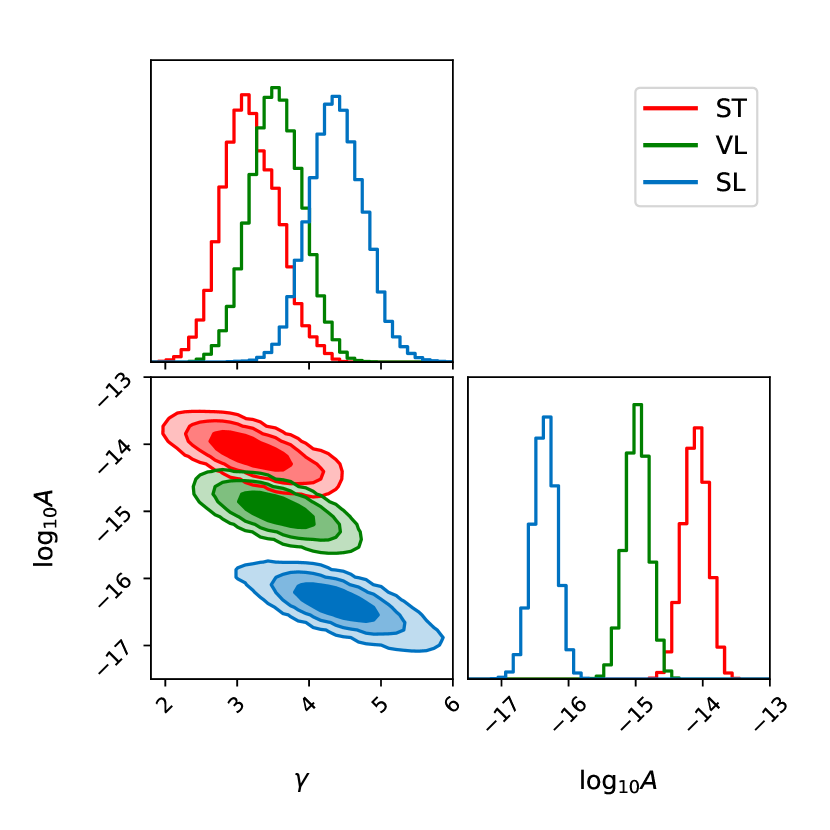
Figure 1: Bayesian posteriors for the amplitude, $A$, and power-law index parameter, $\gamma$, obtained in the ST, VL, and SL models. We show the $1\sigma$, $2\sigma$, and $3\sigma$ contours in the two-dimensional plot.

We also consider a TT+ST model that simultaneously incorporates both the TT and ST correlations. The Bayes factor between the TT+ST model and the TT model is $0.943\pm 0.005$, indicating that there is no significant evidence supporting or refuting the ST correlations in addition to the HD correlations. The contour plot and the posterior distributions of the TT and ST components in the TT+ST model are depicted in Fig. 2. The presence of the peak around $-14.5$ for the amplitude $\log_{10}A_{\mathrm{ST}}$ confirms that the NANOGrav data does not rule out the possibility of an ST signal in the data.

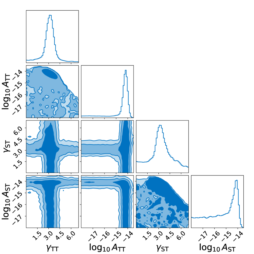
Figure 2: Same as Fig. 1 but for the TT+ST model.

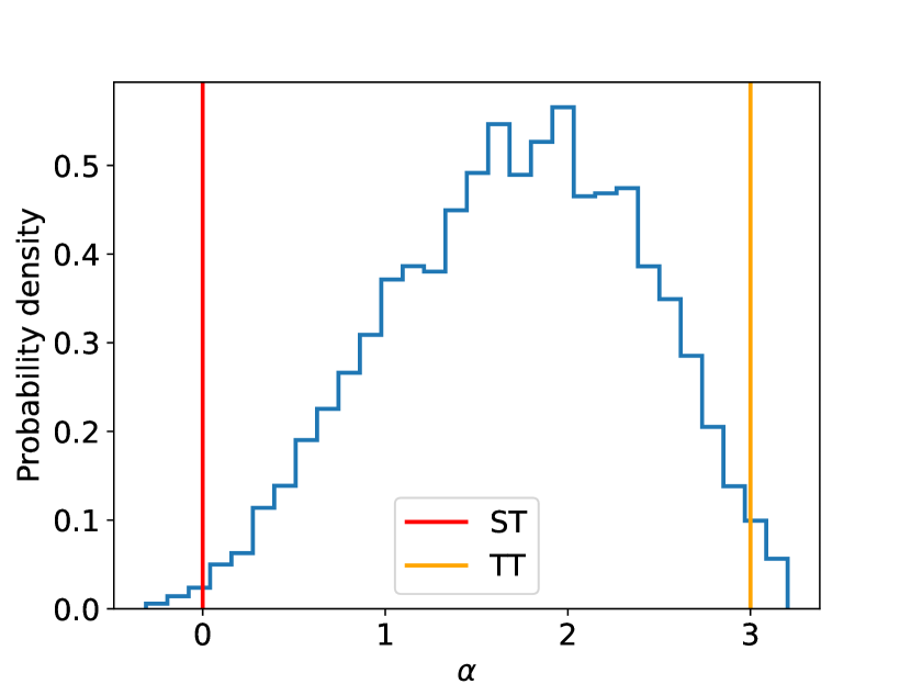
Figure 3: Bayesian posteriors for the $\alpha$ parameter in the GT model with a parameterized ORF as defined by Eq. (10). The two vertical dashed lines correspond to the ST ($\alpha=0$) and TT ($\alpha=3$) ORFs, respectively.

To gain further insights into the optimal correlations that best describe the data, we also fit the NANOGrav 15-year data set with a parameterized ORF (the GT model) as defined in Eq. (10). The posterior distribution for the free parameter $\alpha$ is displayed in Fig. 3. Our analysis yields a value of $\alpha=1.74^{+1.18}_{-1.41}$, thus excluding both the TT ($\alpha=3$) and ST ($\alpha=0$) models at the $90\%$ confidence level. However, it is worth noting that the TT and ST models remain consistent with the NANOGrav 15-year data set at the $3\sigma$ confidence level. Furthermore, the Bayes factor between the GT-best model, where $\alpha$ is set to the best-fit value, and the TT model is $3.9\pm 0.3$, confirming that NANOGrav can be better described by the correlations with $\alpha\simeq 1.7$ than by the HD correlations with $\alpha=3$.

In summary, our analysis indicates that the NANOGrav 15-year data set can be effectively described by either the TT correlations or the ST correlations. No compelling evidence exists to strongly favour one over the other. The current PTA data cannot provide a definitive verdict on the spatial correlations within the stochastic signal, thereby posing a challenge for the unequivocal detection of the GWB predicted by general relativity through PTAs. Future work may need to consider the potential impact of cosmic variance in this pursuit Allen (2023); Allen and Romano (2023); Bernardo and Ng (2022, 2023c, 2023d, 2023e). We anticipate that future PTA data with a longer observation timespan and a larger number of pulsars will provide the necessary insights to pinpoint the origin of the observed stochastic signal.

Note added. A similar study by the NANOGrav collaboration Agazie et al. (2023f), which explores transverse polarization modes in their 15-year data set, was posted on arXiv one day after our manuscript. While the results regarding the ST mode from Ref. Agazie et al. (2023f) are largely consistent with our findings, it is worth highlighting that our study investigates the SL, VL, and GT models that were not examined in Ref. Agazie et al. (2023f).

Acknowledgments We acknowledge the use of the HPC Cluster of ITP-CAS. QGH is supported by grants from NSFC (Grant No. 12250010, 11975019, 11991052, 12047503), Key Research Program of Frontier Sciences, CAS, Grant No. ZDBS-LY-7009, the Key Research Program of the Chinese Academy of Sciences (Grant No. XDPB15). ZCC is supported by the National Natural Science Foundation of China (Grant No. 12247176 and No. 12247112) and the China Postdoctoral Science Foundation Fellowship No. 2022M710429.

References

- Sazhin (1978) M. V. Sazhin, Soviet Astronomy 22, 36 (1978).
- Detweiler (1979) S. L. Detweiler, Astrophys. J. 234, 1100 (1979).
- Foster and Backer (1990) R. S. Foster and D. C. Backer, Astrophys. J. 361, 300 (1990).
- Kramer and Champion (2013) M. Kramer and D. J. Champion (EPTA), Class. Quant. Grav. 30, 224009 (2013).
- McLaughlin (2013) M. A. McLaughlin, Class. Quant. Grav. 30, 224008 (2013), arXiv:1310.0758 [astro-ph.IM] .
- Manchester et al. (2013) R. N. Manchester et al., Publ. Astron. Soc. Austral. 30, 17 (2013), arXiv:1210.6130 [astro-ph.IM] .
- Joshi et al. (2018) B. C. Joshi, P. Arumugasamy, M. Bagchi, et al., Journal of Astrophysics and Astronomy 39, 51 (2018).
- Hobbs et al. (2010) G. Hobbs et al., Class. Quant. Grav. 27, 084013 (2010), arXiv:0911.5206 [astro-ph.SR] .
- Manchester (2013) R. N. Manchester, Class. Quant. Grav. 30, 224010 (2013), arXiv:1309.7392 [astro-ph.IM] .
- Lee (2016) K. J. Lee, in Frontiers in Radio Astronomy and FAST Early Sciences Symposium 2015, Astronomical Society of the Pacific Conference Series, Vol. 502, edited by L. Qain and D. Li (2016) p. 19.
- Miles et al. (2023) M. T. Miles et al., Mon. Not. Roy. Astron. Soc. 519, 3976 (2023), arXiv:2212.04648 [astro-ph.HE] .
- Agazie et al. (2023a) G. Agazie et al. (NANOGrav), Astrophys. J. Lett. 951, L9 (2023a), arXiv:2306.16217 [astro-ph.HE] .
- Agazie et al. (2023b) G. Agazie et al. (NANOGrav), Astrophys. J. Lett. 951, L8 (2023b), arXiv:2306.16213 [astro-ph.HE] .
- Antoniadis et al. (2023a) J. Antoniadis et al. (EPTA), Astron. Astrophys. 678, A48 (2023a), arXiv:2306.16224 [astro-ph.HE] .
- Antoniadis et al. (2023b) J. Antoniadis et al. (EPTA), Astron. Astrophys. 678, A50 (2023b), arXiv:2306.16214 [astro-ph.HE] .
- Zic et al. (2023) A. Zic et al., (2023), arXiv:2306.16230 [astro-ph.HE] .
- Reardon et al. (2023) D. J. Reardon et al., Astrophys. J. Lett. 951, L6 (2023), arXiv:2306.16215 [astro-ph.HE] .
- Xu et al. (2023) H. Xu et al., Res. Astron. Astrophys. 23, 075024 (2023), arXiv:2306.16216 [astro-ph.HE] .
- Hellings and Downs (1983) R. w. Hellings and G. s. Downs, Astrophys. J. Lett. 265, L39 (1983).
- Li et al. (2019) J. Li, Z.-C. Chen, and Q.-G. Huang, Sci. China Phys. Mech. Astron. 62, 110421 (2019), [Erratum: Sci.China Phys.Mech.Astron. 64, 250451 (2021)], arXiv:1907.09794 [astro-ph.CO] .
- Vagnozzi (2021) S. Vagnozzi, Mon. Not. Roy. Astron. Soc. 502, L11 (2021), arXiv:2009.13432 [astro-ph.CO] .
- Chen et al. (2021) Z.-C. Chen, C. Yuan, and Q.-G. Huang, Sci. China Phys. Mech. Astron. 64, 120412 (2021), arXiv:2101.06869 [astro-ph.CO] .
- Wu et al. (2022a) Y.-M. Wu, Z.-C. Chen, and Q.-G. Huang, Astrophys. J. 925, 37 (2022a), arXiv:2108.10518 [astro-ph.CO] .
- Chen et al. (2022a) Z.-C. Chen, Y.-M. Wu, and Q.-G. Huang, Commun. Theor. Phys. 74, 105402 (2022a), arXiv:2109.00296 [astro-ph.CO] .
- Benetti et al. (2022) M. Benetti, L. L. Graef, and S. Vagnozzi, Phys. Rev. D 105, 043520 (2022), arXiv:2111.04758 [astro-ph.CO] .
- Chen et al. (2022b) Z.-C. Chen, Y.-M. Wu, and Q.-G. Huang, Astrophys. J. 936, 20 (2022b), arXiv:2205.07194 [astro-ph.CO] .
- Ashoorioon et al. (2022) A. Ashoorioon, K. Rezazadeh, and A. Rostami, Phys. Lett. B 835, 137542 (2022), arXiv:2202.01131 [astro-ph.CO] .
- Wu et al. (2022b) Y.-M. Wu, Z.-C. Chen, Q.-G. Huang, X. Zhu, N. D. R. Bhat, Y. Feng, G. Hobbs, R. N. Manchester, C. J. Russell, and R. M. Shannon (PPTA), Phys. Rev. D 106, L081101 (2022b), arXiv:2210.03880 [astro-ph.CO] .
- Wu et al. (2023a) Y.-M. Wu, Z.-C. Chen, and Q.-G. Huang, Phys. Rev. D 107, 042003 (2023a), arXiv:2302.00229 [gr-qc] .
- Falxa et al. (2023) M. Falxa et al. (IPTA), Mon. Not. Roy. Astron. Soc. 521, 5077 (2023), arXiv:2303.10767 [gr-qc] .
- Wu et al. (2023b) Y.-M. Wu, Z.-C. Chen, and Q.-G. Huang, JCAP 09, 021 (2023b), arXiv:2305.08091 [hep-ph] .
- Dandoy et al. (2023) V. Dandoy, V. Domcke, and F. Rompineve, SciPost Phys. Core 6, 060 (2023), arXiv:2302.07901 [astro-ph.CO] .
- Madge et al. (2020) E. Madge, E. Morgante, C. Puchades-Ibáñez, N. Ramberg, W. Ratzinger, S. Schenk, and P. Schwaller, JHEP 23, 171 (2020), arXiv:2306.14856 [hep-ph] .
- Bi et al. (2023a) Y.-C. Bi, Y.-M. Wu, Z.-C. Chen, and Q.-G. Huang, (2023a), arXiv:2310.08366 [astro-ph.CO] .
- Wu et al. (2023c) Y.-M. Wu, Z.-C. Chen, Y.-C. Bi, and Q.-G. Huang, (2023c), arXiv:2310.07469 [astro-ph.CO] .
- Afzal et al. (2023) A. Afzal et al. (NANOGrav), Astrophys. J. Lett. 951, L11 (2023), arXiv:2306.16219 [astro-ph.HE] .
- Antoniadis et al. (2023c) J. Antoniadis et al. (EPTA), (2023c), arXiv:2306.16227 [astro-ph.CO] .
- King et al. (2023) S. F. King, D. Marfatia, and M. H. Rahat, (2023), arXiv:2306.05389 [hep-ph] .
- Niu and Rahat (2023) X. Niu and M. H. Rahat, (2023), arXiv:2307.01192 [hep-ph] .
- Ben-Dayan et al. (2023) I. Ben-Dayan, U. Kumar, U. Thattarampilly, and A. Verma, (2023), arXiv:2307.15123 [astro-ph.CO] .
- Vagnozzi (2023) S. Vagnozzi, JHEAp 39, 81 (2023), arXiv:2306.16912 [astro-ph.CO] .
- Fu et al. (2023) C. Fu, J. Liu, X.-Y. Yang, W.-W. Yu, and Y. Zhang, (2023), arXiv:2308.15329 [astro-ph.CO] .
- Agazie et al. (2023c) G. Agazie et al. (International Pulsar Timing Array), (2023c), arXiv:2309.00693 [astro-ph.HE] .
- Basilakos et al. (2023a) S. Basilakos, D. V. Nanopoulos, T. Papanikolaou, E. N. Saridakis, and C. Tzerefos, (2023a), arXiv:2309.15820 [astro-ph.CO] .
- Bian et al. (2023) L. Bian, S. Ge, J. Shu, B. Wang, X.-Y. Yang, and J. Zong, (2023), arXiv:2307.02376 [astro-ph.HE] .
- Wu et al. (2023d) Y.-M. Wu, Z.-C. Chen, and Q.-G. Huang, (2023d), arXiv:2307.03141 [astro-ph.CO] .
- Ellis et al. (2023a) J. Ellis, M. Fairbairn, G. Franciolini, G. Hütsi, A. Iovino, M. Lewicki, M. Raidal, J. Urrutia, V. Vaskonen, and H. Veermäe, (2023a), arXiv:2308.08546 [astro-ph.CO] .
- Figueroa et al. (2023) D. G. Figueroa, M. Pieroni, A. Ricciardone, and P. Simakachorn, (2023), arXiv:2307.02399 [astro-ph.CO] .
- Agazie et al. (2023d) G. Agazie et al. (NANOGrav), Astrophys. J. Lett. 952, L37 (2023d), arXiv:2306.16220 [astro-ph.HE] .
- Ellis et al. (2023b) J. Ellis, M. Fairbairn, G. Hütsi, J. Raidal, J. Urrutia, V. Vaskonen, and H. Veermäe, (2023b), arXiv:2306.17021 [astro-ph.CO] .
- Shen et al. (2023) Z.-Q. Shen, G.-W. Yuan, Y.-Y. Wang, and Y.-Z. Wang, (2023), arXiv:2306.17143 [astro-ph.HE] .
- Bi et al. (2023b) Y.-C. Bi, Y.-M. Wu, Z.-C. Chen, and Q.-G. Huang, (2023b), arXiv:2307.00722 [astro-ph.CO] .
- Barausse et al. (2023) E. Barausse, K. Dey, M. Crisostomi, A. Panayada, S. Marsat, and S. Basak, (2023), arXiv:2307.12245 [astro-ph.GA] .
- Kitajima et al. (2023) N. Kitajima, J. Lee, K. Murai, F. Takahashi, and W. Yin, (2023), arXiv:2306.17146 [hep-ph] .
- Blasi et al. (2023) S. Blasi, A. Mariotti, A. Rase, and A. Sevrin, (2023), arXiv:2306.17830 [hep-ph] .
- Babichev et al. (2023) E. Babichev, D. Gorbunov, S. Ramazanov, R. Samanta, and A. Vikman, (2023), arXiv:2307.04582 [hep-ph] .
- Kitajima and Nakayama (2023) N. Kitajima and K. Nakayama, Phys. Lett. B 846, 138213 (2023), arXiv:2306.17390 [hep-ph] .
- Ellis et al. (2023c) J. Ellis, M. Lewicki, C. Lin, and V. Vaskonen, (2023c), arXiv:2306.17147 [astro-ph.CO] .
- Wang et al. (2023a) Z. Wang, L. Lei, H. Jiao, L. Feng, and Y.-Z. Fan, (2023a), arXiv:2306.17150 [astro-ph.HE] .
- Antusch et al. (2023) S. Antusch, K. Hinze, S. Saad, and J. Steiner, (2023), arXiv:2307.04595 [hep-ph] .
- Ahmed et al. (2023a) W. Ahmed, T. A. Chowdhury, S. Nasri, and S. Saad, (2023a), arXiv:2308.13248 [hep-ph] .
- Ahmed et al. (2023b) W. Ahmed, M. U. Rehman, and U. Zubair, (2023b), arXiv:2308.09125 [hep-ph] .
- Basilakos et al. (2023b) S. Basilakos, D. V. Nanopoulos, T. Papanikolaou, E. N. Saridakis, and C. Tzerefos, (2023b), arXiv:2307.08601 [hep-th] .
- Chen et al. (2023a) Z.-C. Chen, Q.-G. Huang, C. Liu, L. Liu, X.-J. Liu, Y. Wu, Y.-M. Wu, Z. Yi, and Z.-Q. You, (2023a), arXiv:2310.00411 [astro-ph.IM] .
- Addazi et al. (2023) A. Addazi, Y.-F. Cai, A. Marciano, and L. Visinelli, (2023), arXiv:2306.17205 [astro-ph.CO] .
- Athron et al. (2023) P. Athron, A. Fowlie, C.-T. Lu, L. Morris, L. Wu, Y. Wu, and Z. Xu, (2023), arXiv:2306.17239 [hep-ph] .
- Zu et al. (2023) L. Zu, C. Zhang, Y.-Y. Li, Y.-C. Gu, Y.-L. S. Tsai, and Y.-Z. Fan, (2023), arXiv:2306.16769 [astro-ph.HE] .
- Jiang et al. (2023) S. Jiang, A. Yang, J. Ma, and F. P. Huang, (2023), arXiv:2306.17827 [hep-ph] .
- Xiao et al. (2023) Y. Xiao, J. M. Yang, and Y. Zhang, (2023), arXiv:2307.01072 [hep-ph] .
- Abe and Tada (2023) K. T. Abe and Y. Tada, (2023), arXiv:2307.01653 [astro-ph.CO] .
- Gouttenoire (2023) Y. Gouttenoire, Phys. Rev. Lett. 131, 171404 (2023), arXiv:2307.04239 [hep-ph] .
- An et al. (2023) H. An, B. Su, H. Tai, L.-T. Wang, and C. Yang, (2023), arXiv:2308.00070 [astro-ph.CO] .
- Cai et al. (2020) R.-G. Cai, Z.-K. Guo, J. Liu, L. Liu, and X.-Y. Yang, JCAP 06, 013 (2020), arXiv:1912.10437 [astro-ph.CO] .
- Yuan et al. (2019) C. Yuan, Z.-C. Chen, and Q.-G. Huang, Phys. Rev. D 100, 081301 (2019), arXiv:1906.11549 [astro-ph.CO] .
- Yuan et al. (2020a) C. Yuan, Z.-C. Chen, and Q.-G. Huang, Phys. Rev. D 101, 043019 (2020a), arXiv:1910.09099 [astro-ph.CO] .
- Chen et al. (2020) Z.-C. Chen, C. Yuan, and Q.-G. Huang, Phys. Rev. Lett. 124, 251101 (2020), arXiv:1910.12239 [astro-ph.CO] .
- Yuan et al. (2020b) C. Yuan, Z.-C. Chen, and Q.-G. Huang, Phys. Rev. D 101, 063018 (2020b), arXiv:1912.00885 [astro-ph.CO] .
- Liu et al. (2023a) L. Liu, X.-Y. Yang, Z.-K. Guo, and R.-G. Cai, JCAP 01, 006 (2023a), arXiv:2112.05473 [astro-ph.CO] .
- Franciolini et al. (2023) G. Franciolini, A. Iovino, Junior., V. Vaskonen, and H. Veermae, (2023), arXiv:2306.17149 [astro-ph.CO] .
- Jin et al. (2023) J.-H. Jin, Z.-C. Chen, Z. Yi, Z.-Q. You, L. Liu, and Y. Wu, JCAP 09, 016 (2023), arXiv:2307.08687 [astro-ph.CO] .
- Liu et al. (2023b) L. Liu, Z.-C. Chen, and Q.-G. Huang, (2023b), arXiv:2307.14911 [astro-ph.CO] .
- Yi et al. (2023a) Z. Yi, Z.-Q. You, Y. Wu, Z.-C. Chen, and L. Liu, (2023a), arXiv:2308.14688 [astro-ph.CO] .
- Harigaya et al. (2023) K. Harigaya, K. Inomata, and T. Terada, (2023), arXiv:2309.00228 [astro-ph.CO] .
- Zhao et al. (2023) Z.-C. Zhao, Q.-H. Zhu, S. Wang, and X. Zhang, (2023), arXiv:2307.13574 [astro-ph.CO] .
- Balaji et al. (2023) S. Balaji, G. Domènech, and G. Franciolini, JCAP 10, 041 (2023), arXiv:2307.08552 [gr-qc] .
- Wang et al. (2023b) S. Wang, Z.-C. Zhao, J.-P. Li, and Q.-H. Zhu, (2023b), arXiv:2307.00572 [astro-ph.CO] .
- Firouzjahi and Talebian (2023) H. Firouzjahi and A. Talebian, JCAP 10, 032 (2023), arXiv:2307.03164 [gr-qc] .
- Wang et al. (2023c) S. Wang, Z.-C. Zhao, and Q.-H. Zhu, (2023c), arXiv:2307.03095 [astro-ph.CO] .
- Cai et al. (2023) Y.-F. Cai, X.-C. He, X.-H. Ma, S.-F. Yan, and G.-W. Yuan, (2023), 10.1016/j.scib.2023.10.027, arXiv:2306.17822 [gr-qc] .
- Liu et al. (2023c) L. Liu, Z.-C. Chen, and Q.-G. Huang, (2023c), arXiv:2307.01102 [astro-ph.CO] .
- Yi and Zhu (2022) Z. Yi and Z.-H. Zhu, JCAP 05, 046 (2022), arXiv:2105.01943 [gr-qc] .
- Yi and Fei (2023) Z. Yi and Q. Fei, Eur. Phys. J. C 83, 82 (2023), arXiv:2210.03641 [astro-ph.CO] .
- Yi et al. (2023b) Z. Yi, Z.-Q. You, and Y. Wu, (2023b), arXiv:2308.05632 [astro-ph.CO] .
- You et al. (2023) Z.-Q. You, Z. Yi, and Y. Wu, (2023), arXiv:2307.04419 [gr-qc] .
- Yi et al. (2023c) Z. Yi, Q. Gao, Y. Gong, Y. Wang, and F. Zhang, (2023c), arXiv:2307.02467 [gr-qc] .
- Cang et al. (2023a) J. Cang, Y. Gao, Y. Liu, and S. Sun, (2023a), arXiv:2309.15069 [astro-ph.CO] .
- Liu et al. (2023d) L. Liu, Y. Wu, and Z.-C. Chen, (2023d), arXiv:2310.16500 [astro-ph.CO] .
- Liu et al. (2019a) L. Liu, Z.-K. Guo, and R.-G. Cai, Phys. Rev. D 99, 063523 (2019a), arXiv:1812.05376 [astro-ph.CO] .
- Chen and Huang (2018) Z.-C. Chen and Q.-G. Huang, Astrophys. J. 864, 61 (2018), arXiv:1801.10327 [astro-ph.CO] .
- Chen et al. (2019) Z.-C. Chen, F. Huang, and Q.-G. Huang, Astrophys. J. 871, 97 (2019), arXiv:1809.10360 [gr-qc] .
- Chen and Huang (2020) Z.-C. Chen and Q.-G. Huang, JCAP 08, 039 (2020), arXiv:1904.02396 [astro-ph.CO] .
- Liu et al. (2019b) L. Liu, Z.-K. Guo, and R.-G. Cai, Eur. Phys. J. C 79, 717 (2019b), arXiv:1901.07672 [astro-ph.CO] .
- Liu et al. (2020) L. Liu, Z.-K. Guo, R.-G. Cai, and S. P. Kim, Phys. Rev. D 102, 043508 (2020), arXiv:2001.02984 [astro-ph.CO] .
- Wu (2020) Y. Wu, Phys. Rev. D 101, 083008 (2020), arXiv:2001.03833 [astro-ph.CO] .
- Chen et al. (2022c) Z.-C. Chen, C. Yuan, and Q.-G. Huang, Phys. Lett. B 829, 137040 (2022c), arXiv:2108.11740 [astro-ph.CO] .
- Chen et al. (2023b) Z.-C. Chen, S. P. Kim, and L. Liu, Commun. Theor. Phys. 75, 065401 (2023b), arXiv:2210.15564 [gr-qc] .
- Meng et al. (2023) D.-S. Meng, C. Yuan, and Q.-G. Huang, Sci. China Phys. Mech. Astron. 66, 280411 (2023), arXiv:2212.03577 [astro-ph.CO] .
- Lu et al. (2019) Y. Lu, Y. Gong, Z. Yi, and F. Zhang, JCAP 12, 031 (2019), arXiv:1907.11896 [gr-qc] .
- Gao et al. (2021) Q. Gao, Y. Gong, and Z. Yi, Nucl. Phys. B 969, 115480 (2021), arXiv:2012.03856 [gr-qc] .
- Yi et al. (2021a) Z. Yi, Q. Gao, Y. Gong, and Z.-h. Zhu, Phys. Rev. D 103, 063534 (2021a), arXiv:2011.10606 [astro-ph.CO] .
- Yi et al. (2021b) Z. Yi, Y. Gong, B. Wang, and Z.-h. Zhu, Phys. Rev. D 103, 063535 (2021b), arXiv:2007.09957 [gr-qc] .
- Yi (2023) Z. Yi, JCAP 03, 048 (2023), arXiv:2206.01039 [gr-qc] .
- Liu et al. (2023e) L. Liu, Z.-Q. You, Y. Wu, and Z.-C. Chen, Phys. Rev. D 107, 063035 (2023e), arXiv:2210.16094 [astro-ph.CO] .
- Chen et al. (2023c) Z.-C. Chen, S.-S. Du, Q.-G. Huang, and Z.-Q. You, JCAP 03, 024 (2023c), arXiv:2205.11278 [astro-ph.CO] .
- Zheng et al. (2023) L.-M. Zheng, Z. Li, Z.-C. Chen, H. Zhou, and Z.-H. Zhu, Phys. Lett. B 838, 137720 (2023), arXiv:2212.05516 [astro-ph.CO] .
- Bhaumik et al. (2023) N. Bhaumik, R. K. Jain, and M. Lewicki, (2023), arXiv:2308.07912 [astro-ph.CO] .
- Bousder et al. (2023) M. Bousder, A. Riadsolh, A. E. Fatimy, M. E. Belkacemi, and H. Ez-Zahraouy, (2023), arXiv:2307.10940 [gr-qc] .
- Hosseini Mansoori et al. (2023) S. A. Hosseini Mansoori, F. Felegray, A. Talebian, and M. Sami, JCAP 08, 067 (2023), arXiv:2307.06757 [astro-ph.CO] .
- Gouttenoire et al. (2023) Y. Gouttenoire, S. Trifinopoulos, G. Valogiannis, and M. Vanvlasselaer, (2023), arXiv:2307.01457 [astro-ph.CO] .
- Huang et al. (2023) H.-L. Huang, Y. Cai, J.-Q. Jiang, J. Zhang, and Y.-S. Piao, (2023), arXiv:2306.17577 [gr-qc] .
- Depta et al. (2023) P. F. Depta, K. Schmidt-Hoberg, P. Schwaller, and C. Tasillo, (2023), arXiv:2306.17836 [astro-ph.CO] .
- Cang et al. (2023b) J. Cang, Y.-Z. Ma, and Y. Gao, Astrophys. J. 949, 64 (2023b), arXiv:2210.03476 [astro-ph.CO] .
- Allen et al. (2023) B. Allen, S. Dhurandhar, Y. Gupta, M. McLaughlin, P. Natarajan, R. M. Shannon, E. Thrane, and A. Vecchio, (2023), arXiv:2304.04767 [astro-ph.IM] .
- Lee et al. (2008) K. J. Lee, F. A. Jenet, and R. H. Price, Astrophys. J. 685, 1304 (2008).
- Chamberlin and Siemens (2012) S. J. Chamberlin and X. Siemens, Phys. Rev. D 85, 082001 (2012), arXiv:1111.5661 [astro-ph.HE] .
- Gair et al. (2015) J. R. Gair, J. D. Romano, and S. R. Taylor, Phys. Rev. D 92, 102003 (2015), arXiv:1506.08668 [gr-qc] .
- Boîtier et al. (2020) A. Boîtier, S. Tiwari, L. Philippoz, and P. Jetzer, Phys. Rev. D 102, 064051 (2020), arXiv:2008.13520 [gr-qc] .
- Bernardo and Ng (2023a) R. C. Bernardo and K.-W. Ng, Phys. Lett. B 841, 137939 (2023a), arXiv:2206.01056 [astro-ph.CO] .
- Bernardo and Ng (2023b) R. C. Bernardo and K.-W. Ng, Phys. Rev. D 107, 044007 (2023b), arXiv:2208.12538 [gr-qc] .
- Arzoumanian et al. (2021) Z. Arzoumanian et al. (NANOGrav), Astrophys. J. Lett. 923, L22 (2021), arXiv:2109.14706 [gr-qc] .
- Cornish et al. (2018) N. J. Cornish, L. O’Beirne, S. R. Taylor, and N. Yunes, Phys. Rev. Lett. 120, 181101 (2018), arXiv:1712.07132 [gr-qc] .
- Agazie et al. (2023e) G. Agazie et al. (NANOGrav), Astrophys. J. Lett. 951, L50 (2023e), arXiv:2306.16222 [astro-ph.HE] .
- Thrane and Romano (2013) E. Thrane and J. D. Romano, Phys. Rev. D 88, 124032 (2013), arXiv:1310.5300 [astro-ph.IM] .
- Aghanim et al. (2020) N. Aghanim et al. (Planck), Astron. Astrophys. 641, A6 (2020), [Erratum: Astron.Astrophys. 652, C4 (2021)], arXiv:1807.06209 [astro-ph.CO] .
- Arzoumanian et al. (2016) Z. Arzoumanian et al. (NANOGrav), Astrophys. J. 821, 13 (2016), arXiv:1508.03024 [astro-ph.GA] .
- Park et al. (2021) R. S. Park, W. M. Folkner, J. G. Williams, and D. H. Boggs, The Astronomical Journal 161, 105 (2021).
- Arzoumanian et al. (2018) Z. Arzoumanian et al. (NANOGRAV), Astrophys. J. 859, 47 (2018), arXiv:1801.02617 [astro-ph.HE] .
- Arzoumanian et al. (2020) Z. Arzoumanian et al. (NANOGrav), Astrophys. J. Lett. 905, L34 (2020), arXiv:2009.04496 [astro-ph.HE] .
- Ellis et al. (2020) J. A. Ellis, M. Vallisneri, S. R. Taylor, and P. T. Baker, “Enterprise: Enhanced numerical toolbox enabling a robust pulsar inference suite,” Zenodo (2020).
- Taylor et al. (2021) S. R. Taylor, P. T. Baker, J. S. Hazboun, J. Simon, and S. J. Vigeland, “enterprise_extensions,” (2021), v2.2.0.
- Ellis and van Haasteren (2017) J. Ellis and R. van Haasteren, “jellis18/ptmcmcsampler: Official release,” (2017).
- Aggarwal et al. (2019) K. Aggarwal et al., Astrophys. J. 880, 2 (2019), arXiv:1812.11585 [astro-ph.GA] .
- Allen (2023) B. Allen, Phys. Rev. D 107, 043018 (2023), arXiv:2205.05637 [gr-qc] .
- Allen and Romano (2023) B. Allen and J. D. Romano, Phys. Rev. D 108, 043026 (2023), arXiv:2208.07230 [gr-qc] .
- Bernardo and Ng (2022) R. C. Bernardo and K.-W. Ng, JCAP 11, 046 (2022), arXiv:2209.14834 [gr-qc] .
- Bernardo and Ng (2023c) R. C. Bernardo and K.-W. Ng, (2023c), arXiv:2306.13593 [gr-qc] .
- Bernardo and Ng (2023d) R. C. Bernardo and K.-W. Ng, JCAP 08, 028 (2023d), arXiv:2304.07040 [gr-qc] .
- Bernardo and Ng (2023e) R. C. Bernardo and K.-W. Ng, (2023e), arXiv:2310.07537 [gr-qc] .
- Agazie et al. (2023f) G. Agazie et al. (NANOGrav), (2023f), arXiv:2310.12138 [gr-qc] .