Document-Level In-Context Few-Shot Relation Extraction via Pre-Trained Language Models

Abstract

Relation extraction aims at inferring structured human knowledge from textual documents. State-of-the-art methods based on language models commonly have two limitations: (1) they require named entities to be either given as input or infer them, which introduces additional noise, and (2) they require human annotations of documents. As a remedy, we present a novel framework for document-level in-context few-shot relation extraction via pre-trained language models. We achieve crucial benefits in that we eliminate the need for both named entity recognition and human annotation of documents. Unlike existing methods based on fine-tuning, our framework is flexible in that it can be easily updated for a new set of relations without re-training. We evaluate our framework using DocRED, the largest publicly available dataset for document-level relation extraction, and demonstrate that our framework achieves state-of-the-art performance. Finally, we show that our framework actually performs much better than the original labels from the development set of DocRED. To the best of our knowledge, we are the first to reformulate the document-level relation extraction task as a tailored in-context few-shot learning paradigm.

*supplements

1 Introduction

Relational facts are widely used to represent human knowledge [18, 20, 82]. With the explosion of the web, relational facts have become broadly available through large knowledge bases (KBs) [3, 64, 5, 67] and thereby support many downstream tasks. Examples are commonsense reasoning [34, 37], question answering [43, 11, 76], fact checking [25, 66], and product recommendations [72, 98, 100]. However, relational facts are not readily available in structured form but are commonly embedded in unstructured texts. To this end, methods are needed for relation extraction from text.

State-of-the-art methods for relation extraction leverage pre-trained language models (LMs) and fine-tune them using human-annotated documents. These works can be loosely grouped into two streams. One stream requires named entities (e. g., by specifying the entities of interest with a special token) as input [71, 84, 92, 101, 65, 78, 83, 24, 85]. Another stream avoids the use of named entities as input and, instead, learns the detection of named entities through a tailored training objective [7, 14, 17, 42, 93].

Yet, state-of-the-art methods based on LMs have three main drawbacks that limit their applicability for relation extraction in practice. (1) State-of-the-art methods for relation extraction typically require the named entities to be either given as input or to be inferred via a customized training objective. This introduces additional noise in the relation extraction pipeline and thus hinders the downstream performance. (2) State-of-the-art methods for relation extraction need large amounts of human-annotated documents for training. However, human annotation is costly. (3) State-of-the-art methods are based on LMs that are fine-tuned. As a result, whenever a new type of relation is added to the knowledge base or whenever a better LM is adopted, the entire training process must be repeated. This introduces a huge computational overhead.

There are some recent efforts that use the reasoning abilities of LMs via in-context learning for relation extraction [68, 69]. However, these are designed for sentence-level relation extraction, meaning for a small set of relation types. Hence, due to high computational costs, their scalability to documents is limited (see Table 1). Here, we introduce a novel method to leverage in-context learning for document-level relation extraction.

Our REPLM framework: We introduce a novel framework called REPLM for document-level in-context few-shot relation extraction via pre-trained language models. Our framework leverages the generalization capabilities of pre-trained LMs by reformulating the relation extraction task as a tailored in-context few-shot learning paradigm. Specifically, for a given document, we retrieve sets of the most relevant in-context examples of a corresponding relation and aggregate the outputs in a probabilistic framework.

Contributions:

1. We present a novel framework called REPLM for in-context few-shot relation extraction via pre-trained LMs. To the best of our knowledge, we are the first to reformulate the document-level relation extraction task as a tailored in-context few-shot learning paradigm.

2. Our REPLM framework has key advantages for practice: it eliminates the noise from named entity recognition, it circumvents the need for human annotations, and it is flexible in that it is directly applicable to new relations without re-training.

3. We show that our REPLM framework achieves state-of-the-art performance.

2 Related Work

In-context few-shot learning of LMs: LMs have achieved superior performance in many downstream tasks [4, 12, 40, 56, 6, 31, 57, 70, 79, 80, 50, 75, 94]. Due to the large computational cost of fine-tuning an LM, Brown et al. [6] proposed in-context few-shot learning paradigm to teach an LM a new task at inference time. We provide an overview of applications in Appendix A. However, we are not aware of any earlier work that leveraged the in-context few-shot learning paradigm for document-level relation extraction.

Early research on relation extraction: Early works extracted relations from text via pattern extraction methods [9, 47, 27, 52, 82] and via statistical methods [62, 90, 91, 26, 49, 74, 87, 77, 35]. However, the above methods have only a limited modeling capacity, as compared to neural networks [88, 46, 99, 1, 29, 96, 20]. As shown later, LM-based methods better capture the complex interactions between named entities to classify the relation. A detailed review is in the Appendix A.

Relation extraction via LM: State-of-the-art methods for relation extraction are based on fine-tuning pre-trained LMs. Specifically, these methods use pre-trained LMs such as BERT [12], RoBERTa [40], and SciBERT [4] and fine-tuned them for relation extraction. For instance, Wang et al. [71] fine-tuned BERT to classify the relation between each named entity pair in a sentence. There have been various follow-up works to improve performance by learning complex dependency between named entities [73, 51, 84, 92, 101, 65, 78, 83, 24, 85, 89]. A detailed review is in Appendix A. However, all these works require the named entities to be annotated and provided as input at both training and test time.

Some works relax the requirement of given named entities to facilitate processing the raw documents at test time. As a remedy, these works jointly learn to extract named entities and relations. Examples are SpERT [13], JEREX [14], Seq2Rel [17], UIE [42], and TaG [93]. Their drawback is that multi-step pipelines with named entities recognition propagate the errors to relation extraction [7]. Motivated by this, Cabot and Navigli [7] developed REBEL, an auto-regressive model based on BART [31], which is fine-tuned to output relations as sequences of texts. To the best of our knowledge, REBEL is the only LM-based method without the need for a named entity recognition pipeline and thus represents our main baseline.

Still, the above methods have salient limitations: (1) they (with the exception of REBEL) require named entities to be given or infer them, which is a source of noise; (2) they require large amounts of human annotations; and (3) they require re-training to handle new relations.

Table 1: Comparison of relevant relation extraction methods.

Method	Scope	Pre-trained LM	Open source	No need for fine-tuning.	No need for named entities.
Wan et al. [69]	Sentence	OpenAI’s GPT	✓	✗	✗
Wadhwa et al. [68]	Sentence	OpenAI’s GPT	✗	✗	✓
REBEL (Cabot et al., 2021)	Document	BART-large	✓	✗	✓
REPLM (ours)	Document	GPT-J	✓	✓	✓

In-context learning for sentence-level relation extraction:. There are two recent works that leverage in-context learning for sentencel-level relation extraction (see Table 1).Wan et al. [69] requires named entities to be provided for each sentence and generates $k$ different chain-of-thought (CoT) reasonings [80] from GPT-3 [6] as in-context examples for each named entity pairs to classify the relation between them. Similarly, Wadhwa et al. [68] requires CoT reasonings from GPT-3 for the entire training corpus and fine-tunes Flan-T5 [10] based on the generated CoT outputs. However, these works are only applicable to a small set of sentences and relation types due to their high computational cost resulting from commercial architectures. Because of that, these methods work only at the sentence-level relation extraction (i. e., they are not scalable to document-level).

Research gap: To the best of our knowledge, no work has adapted the in-context few-shot learning paradigm for document-level relation extraction. This presents our novelty and offers direct benefits in practice (i.e., no need for named entity input, no need for human annotations, and flexible adaptation to new relations without re-training).

3 Problem Description

Relation extraction: The task of relation extraction from the documents is typically defined as follows [71, 14, 84, 92, 101, 17, 42, 65, 78, 85]. Given is a set of documents $\mathcal{D}=\{d_{i}\}_{i=1}^{M}$, where $M$ is the number of documents in the set. For each document $d_{i}$, the aim is to enumerate knowledge triplets $\{(r_{im},s_{im},o_{im})\}_{m=1}^{R_{i}}$, where $r_{im}\in\mathcal{R}$ is a relation and $s_{im}$ and $o_{im}$ are the subject and object of the relation $r_{im}$, and where $R_{i}$ is the number of relations in $d_{i}$. For instance, the document “The Reality Dysfunction is a science fiction novel by British writer Peter F. Hamilton $\ldots$” yields the knowledge triplets (author, The Reality Dysfunction, Peter F. Hamilton), (genre, The Reality Dysfunction, science fiction), etc.

Difference to earlier works: Earlier works (see Sec. 2) generally address the above task through an intermediate step that involves named entities detection. Specifically, the aforementioned works first detect the named entities of a document $d_{i}$, i. e., $\{e_{ij}\}_{j=1}^{N_{i}}$, where $N_{i}$ is the number of entities in $d_{i}$. Then they proceed by predicting the relation(s) between each named entity pair $(e_{ij},e_{ij^{\prime}})_{j,j^{\prime}\in\{1,\ldots,N_{i}\},j\neq j^{\prime}}$ among the $R$ relations, where $e_{ij}$ is the subject and $e_{ij^{\prime}}$ is the object of predicted relation(s). As such, the number of predictions scales with the number of named entity pairs, i.e., it is in $O(N_{i}^{2})$. For the prediction, state-of-the-art methods make use of pre-trained LMs for which a multi-class classification head is fine-tuned. The classification head also predicts when there is no relation between the given pair and then discards the knowledge triplet. All remaining relations give the knowledge triplets $\{(r_{im},s_{im},o_{im})\}_{m=1}^{R_{i}}$.

In-context few-shot learning in REPLM: Our REPLM framework addresses the above drawbacks and approaches relation extraction as a triplet generation task. In this setup, the LM learns how to generate subject(s) and object(s) of a given relation from its in-context few-shot examples. Therefore, our REPLM framework does not require annotations of named entities. Our setup also facilitates the flexibility of adding new relations, simply by leveraging the given context examples. Specifically, for a given document $d_{i}\in\mathcal{D}$ and relation $r\in\mathcal{R}$, we prompt a pre-trained LM to generate the knowledge triplets of a relation $\{(r_{im},s_{im},o_{im})\,|\,r_{im}=r\}$ with no further fine-tuning.

In our REPLM framework, we have two sets of documents as input: (1) a distantly-supervised set $\mathcal{D}^{\text{dist}}$ for providing in-context few-shot examples and (2) a training set $\mathcal{D}^{\text{train}}$ for calibrating hyperparameters (which is optional). Details are in the next section.

4 Proposed REPLM Framework

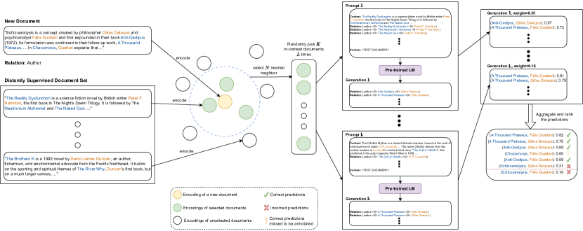
Figure 1: Overview of our REPLM. Our framework takes a new document and relation as input and then proceeds along three steps: (1) selects a candidate pool of $N$ in-context examples; (2) constructs $L$ sets of such in-context examples; and (3) calculates the joint probabilities of subject-object pairs to extract knowledge triplets. Legend: subjects and objects are colored in blue and orange, respectively.

Approach (see Fig. 1): At a high-level, our framework seeks to infer the correct knowledge triplets $(r,s,o)$ from a given document $d_{i}$ and for a given relation $r$. To do so, we estimate the joint probability of a subject-object pair $(s,o)$ conditional on $d_{i}$ and $r$, i.e., $p(s,o\,|\,d_{i},r)$. After having estimated the probability, we simply rank the candidate subject-object pairs according to their probabilities and keep the top-ranked pairs as knowledge triplets. In our framework, we follow this approach but, as a main innovation, leverage a pre-trained LM to approximate $p(s,o\,|\,d_{i},r)$.

Learning via in-context few-shot examples: Pre-trained LMs are not explicitly trained for our relation extraction task, although they generally have the ability to extract information from a given context when guided properly. In our framework, we intentionally avoid the use of fine-tuning a pre-trained LM due to high computational cost and the inability of handling new relations. Instead, we provide guidance for our task via in-context few-shot examples. These examples demonstrate how to extract the subject-object pairs of relation $r$ from the given context. As a result, we can approximate $p(s,o\,|\,d_{i},r)\sim p(s,o\,|\,C,d_{i},r)$, where $C$ represents the selected set of in-context examples.

However, selecting only a single set of in-context examples may lead to a poor approximation of the probability $p(s,o\,|\,d_{i},r)$, because the selected in-context examples introduce bias in output generation (e. g., recency bias, label space of the in-context examples) as studied in prior literature [36, 45, 61, 23, 81]. Instead, we mitigate the above bias by considering multiple sets of in-context examples. As a result, we calculate the joint probability of a subject-object pair as

$$p(s,o\,|\,d_{i},r)=\sum_{l=1}^{L}p(C_{l}\,|\,d_{i},r)\cdot p(s,o\,|\,C_{l},d_{i},r),$$ (1)

where we aggregate the outputs from $L$ sets of in-context examples. Here, $p(C_{l}\,|\,d_{i},r)$ is the weight of set $C_{l}$ of in-context examples, which measures how well $C_{l}$ is a candidate set compared to other sets of in-context examples.

Steps: Our REPLM framework proceeds along three steps: (1) it first selects a candidate pool for the in-context examples (Sec. 4.1); (2) it then constructs multiple sets of in-context examples and assigns their weights via a tailored approach (Sec. 4.2); and (3) it calculates the joint probabilities subject-object pairs to extract the knowledge triplets (Sec. 4.3). We describe the steps in the following.

4.1 Selecting Candidates for In-Context Examples

We now create a candidate pool of in-context few-shot examples for a given document $d_{i}$. Crucially, we generate our candidate pool in a way that, on the one hand, it is created via distant supervision and thus without human annotation, and, on the other hand, it is semantically related to the document $d_{i}$, thereby providing meaningful guidance.

Distant supervision: We create the in-context few-shot examples from the set $\mathcal{D}^{\text{dist}}$ generated by distant supervision. Specifically, $\mathcal{D}^{\text{dist}}$ is a dataset without any human annotation. In our implementation, we use the distantly-supervised split of DocRED [86], automatically created via an external knowledge base (KB). Reassuringly, we emphasize that this split comprises documents and knowledge triplets but it was created without any human annotation.

Distant supervision assumes that, if a document $\tilde{d}\in\mathcal{D}^{\text{dist}}$ contains both the subject and object of a knowledge triplet from a KB, it likely discusses their relationship. This premise allows for the automatic generation of annotated document sets. Such automated annotation introduces noisy labels [86, 7], yet that can oftentimes be effective [45]. A key benefit is that distantly supervised documents offer rich insights into label space, textual distributions, and expected output formats, over which the in-context few-shot learning paradigm in our REPLM can generalize.

Semantic filtering: (i) We first filter the documents in $\mathcal{D}^{\text{dist}}$ so that we only keep the documents that contain at least one knowledge triplet of a relation $r$. We denote the result by $\mathcal{D}_{r}^{\text{dist}}$. Formally, $\mathcal{D}_{r}^{\text{dist}}$ is defined as

$$\mathcal{D}_{r}^{\text{dist}}=\{d_{j}\,|\,\exists\,r^{\prime},s,o\ \mathrm{s.t.}\ (r^{\prime},s,o)\in d_{j}\\ \land r^{\prime}=r\land d_{j}\in\mathcal{D}^{\text{dist}}\}.$$

(ii) We then retrieve $N$ documents from $\mathcal{D}_{r}^{\text{dist}}$ that are semantically most similar to $d_{i}$. For this, we leverage the technique from [36] and encode the document $d_{i}$ and all the documents $\{d_{j}\,|\,d_{j}\in\mathcal{D}_{r}^{\text{dist}}\}$ into their embeddings via encoder $F_{\theta}$. (iii) We calculate the cosine similarity between the embeddings of $d_{i}$ and $d_{j}$, i.e., $\frac{F_{\theta}(d_{i})\cdot F_{\theta}(d_{j})}{||F_{\theta}(d_{i})||_{2}\cdot||F_{\theta}(d_{j})||_{2}}$. (iv) We keep the top-$N$ documents in $\mathcal{D}_{r}^{\text{dist}}$ in terms of cosine similarity to $d_{i}$ in embedding space. The selected $N$ documents form the context pool $\mathcal{D}_{r}^{\text{pool}}$, from which we construct multiple sets of in-context examples in the following.

4.2 Constructing Multiple Sets of In-Context Examples

For robustness, we create $L$ sets with in-context examples from our candidate pool $\mathcal{D}_{r}^{\text{pool}}$. We achieve this by random sampling of $K$ documents from $\mathcal{D}_{r}^{\text{pool}}$ across $L$ repetitions. As a result, we obtain $L$ sets of in-context examples, i.e., $C_{1},\ldots,C_{L}$. Then, we perform weighting at the set level.

Weighting at set level: The output from each context set $C_{l}$ should contribute to the relation extraction task proportional to some weight $p(C_{l}\,|\,d_{i},r)$. We calculate the weight as follows. First, we get a score for $C_{l}$ which is the average cosine similarity between the documents in $C_{l}$ and $d_{i}$, i. e.,

$$\mathrm{score}(C_{l})=\frac{1}{K}\sum_{d_{j}\in C_{l}}\frac{F_{\theta}(d_{i})\cdot F_{\theta}(d_{j})}{||F_{\theta}(d_{i})||_{2}\cdot||F_{\theta}(d_{j})||_{2}}.$$ (2)

We then use the score of $C_{l}$ to calculate the weight via

$$p(C_{l}\,|\,d_{i},r)=\frac{\mathrm{exp}(\mathrm{score}(C_{l})/\tau)}{\sum_{l^{\prime}=1}^{L}\mathrm{exp}(\mathrm{score}(C_{l^{\prime}})/\tau)},$$ (3)

where $\tau>0$ is for temperature scaling. Hence, $p(C_{l}\,|\,d_{i},r)$ represents how much the final output of REPLM should attend to the output generated from the context set $C_{l}$.

4.3 Computing Knowledge Triplet Probabilities

We now calculate the probabilities for subject-object pairs and then extract the knowledge triplets.

Prompting: We prompt our pre-trained LM with both (i) the in-context few-shot examples derived from $C_{l}$ and (ii) the document $d_{i}$ at the end of the prompt. For this, we first prepare the in-context demonstrations for each context set $C_{l}$. That is, we concatenate the documents $d_{j}$ in $C_{l}$, where each document $d_{j}$ is appended with its corresponding knowledge triplets $\{(r_{jm},s_{jm},o_{jm})\,|\,r_{jm}=r\}$. Each knowledge triplet is added in a new line (see Fig. 1). For the textual prompt, we separate the relation, subject, and object of $(r,s,o)$ with a special separator symbol <S>. This facilitates easier parsing of the subjects and objects generated.

Calculation of joint probability: We first obtain the log probabilities of both subject and object tokens under our pre-trained LM. We normalize the log probabilities by the length (i. e., number of tokens) of the subject and object. Formally, we compute (here: we directly write the exponent of the average log. probabilities for the ease of reading):

$$p(s\,|\,C_{l},d_{i},r) =\sqrt[\mathrm{len}(s)]{\prod_{k=1}^{\mathrm{len}(s)}p(s_{k}\,|\,s_{<k},C_{l},d_{i},r)},$$ (4)

$$p(o\,|\,s,C_{l},d_{i},r) =\sqrt[\mathrm{len}(o)]{\prod_{k=1}^{\mathrm{len}(o)}p(o_{k}\,|\,o_{<k},s,C_{l},d_{i},r)},$$ (5)

where $\mathrm{len}(s)$ and $\mathrm{len}(o)$ are the number of tokens of the subject and object, respectively. Afterward, we compute the joint probability $p(s,o\,|\,C_{l},d_{i},r)=p(s\,|\,C_{l},d_{i},r)\cdot p(o\,|\,s,C_{l},d_{i},r)$.

Ranking: As the final step, we calculate $p(s,o\,|\,d_{i},r)$ by aggregating over the context sets $C_{l}$, $l=1,\ldots,L$, as in Eq. (1) and repeat this for all generated subject-object pairs. We keep all generated knowledge triplets whose probability exceeds a certain threshold $\theta$, i. e., $\{(r,s,o)\,|\,p(s,o\,|\,d_{i},r)>\theta\}$. Of note, if a subject-object pair is not generated from a context set $C_{l}$, then $p(s,o\,|\,C_{l},d_{i},r)=0$.

Note that the latter step is different from state-of-the-art methods as these methods must enumerate over all possible subject-object pairs. Further, as can be seen here, our framework does not require named entities as input, which is another salient difference to many of the existing works.

5 Experimental Setup

We evaluate our framework using the DocRED [86], the largest document-level relation extraction dataset publicly available. DocRED includes 96 relation types and comprises three sets: (1) a distantly-supervised set with 101,873 documents, (2) a human-annotated train set with 3053 documents, and (3) a human-annotated development set with 998 documents. We provide further details about the DocRED dataset in the Appendix B. Importantly, in our experimental setup, we use distantly-supervised set for in-context few-shot learning ($\mathcal{D}^{\text{dist}}$) and evaluate the performance on the development set. Thereby, we ensure that our framework is solely trained without human annotation. To better understand the performance of our REPLM, we thus later also perform additional experiments (see Sec. 7) using sentence-level relation extraction datasets.

Baselines. We evaluate our framework against state-of-the-art methods for relation extraction that scale to document-level and, for comparability, do not require named entity recognition pipelines (see Table 1). These are: (1) REBEL [7] applies triplet linearization to extract the relations from the given document. (2) We also compare against REBEL-sent, which extracts the relations from a document in sentence-by-sentence manner. We include this variant because REBEL is originally trained at sentence level and, as we show later, it is the best-performing baseline method for the sentence-level relation extraction. Note that REBEL is the only baseline from the literature that does not require a named entity recognition pipeline for document-level relation extraction.

In our dataset, we use REBEL-large from Hugging Face, which is pre-trained by a tailored REBEL dataset. We note that REBEL-large is further fine-tuned on the human-annotated training set of DocRED, which may give it an (unfair) advantage. Hyperparameter selection and early-stopping are done based on some portion of the development set. This is again an (unfair) advantage for REBEL, whereas our REPLM does not need such dev set.

REPLM variants: We compare two variants of our proposed framework: (1) REPLM is the original variant as described above. Therein, we use fixed parameters. We also report a sensitivity analysis in Appendix J, where we vary the parameters to see that our performance is robust to different choices. (2) REPLM (params adj) is a variant for which the hyperparameters (e. g., temperature, threshold) are selected based on the training set.

Ablations: We perform ablation studies to assess the contribution of different components in our framework. Our ablations are: (1) REPLM (random fixed) randomly selects a single set of $K$ documents for each relation. However, the set is fixed across all evaluations. (2) REPLM (random all) randomly selects a set of $K$ documents for each relation and for each evaluation. (3) REPLM (best context$\ominus$) selects the top-$K$ documents for each relation and each development document according to the cosine similarity. In-context examples are ordered from most similar to the least similar. (4) REPLM (best context$\oplus$) similarly selects top $K$ documents for each relation and each development document. This time, in-context examples are ordered in reverse order, from least similar to most similar. We include these two alternatives to evaluate the effect (if any) of recency bias [41, 23].

Evaluation. We calculate the F1 score for each relation, counting an extraction as correct only if the subject and object exactly align with the ground-truth. Thus, extracted relations missing in the development set are false positives, while those in the set but not generated are false negatives.

Implementation. We use GPT-JT ($\sim$6B parameters) as our pre-trained LM for in-context few-shot learning. Appendix E provides all details of our REPLM framework.

6 Results

6.1 Overall Performance

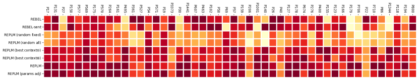
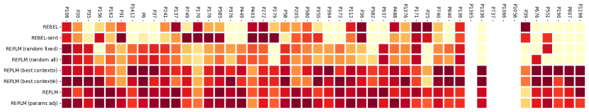
Figure 2: F1 scores per relation type (darker = better). Missing color means that no correct predictions were made for this relation. F1 scores are normalized by the maximum value for each relation. Relations are in decreasing order of their number of knowledge triplets.

First, we evaluate how accurately our REPLM framework extracts the relations from the given documents by comparing them against human annotations (Fig. 2). Overall, our REPLM and REPLM (params adj) achieve state-of-the-art performance on most relation types. This pattern is especially pronounced for relations with a large number of knowledge triplets (e.g., P17: country, P131: located in, P27: country of citizenship).

Table 2: Document-level relation extraction results. Shown: Micro F1 scores.

Method	F1 score
REBEL (Cabot et al., 2021)	26.17
REBEL-sent (Cabot et al., 2021)	27.52
REPLM (random fixed)	21.04  $\pm$  0.17
REPLM (random all)	21.14  $\pm$  0.09
REPLM (best context$\ominus$)	31.31
REPLM (best context$\oplus$)	31.04
REPLM (ours)	33.93
REPLM (params adj) (ours)	35.09
Higher is better. Best value in bold.

Table 2 reports the overall performance, i.e., the micro F1 score over all relation types. Our REPLM achieves an F1 score of 33.93, and our REPLM (params adj) an F1 score of 35.09. The slight advantage of the latter is expected and can be attributed to the additional hyperparameter tuning. For comparison, the REBEL-sent baseline registers only an F1 score of 27.52. In sum, our framework performs the best and results in an improvement of +27 %. Note that REBEL was even fine-tuned on some samples of the dev set, which again demonstrates the clear superiority of our framework. We observe that REPLM outputs, on average, 20.21 knowledge triplets per document while REBEL outputs only 4.93; we discuss the implications later.

In our ablation study, we compare different variants of our REPLM to understand the source of performance gains (see Fig. 2 and Table 2). We make the following observations: (1) Retrieving the best in-context examples improves the performance compared to random examples by more than 48 % (REPLM (best context$\ominus$) and REPLM (best context$\oplus$) vs. REPLM (random fixed) and REPLM (random all)). (2) We do not observe that a recency bias plays a decisive role for our results, as both REPLM (best context$\ominus$) and REPLM (best context$\oplus$) reach a similar performance. (3) Our complete framework brings a significant improvement over REPLM (best context$\ominus$) and REPLM (best context$\oplus$) (+18 %) by aggregating multiple sets of most relevant in-context examples, thus establishing the importance of using multiple sets.

Insights. We conjecture that our REPLM extracts more relations than REBEL, as it further identifies the missing annotations in DocRED. In Appendix F, we empirically validate that, for each relation type, there are dev documents with no annotation, which are semantically similar to the documents containing at least one knowledge triplet of a relation. It suggests that these dev documents potentially include the relation but lack the annotation. To confirm this conjecture, we perform a manual validation that we examine cases where our REPLM fails. We find that many relations extracted by our method are actually correct but considered as false positives due to missing human annotations. For example, our REPLM generates the relation (author, Chaosmosis, Félix Guattari) but it is not annotated and therefore marked as incorrect (see right part of Fig. 1). We provide additional examples in the Appendix G.

6.2 Comparison Against External Knowledge

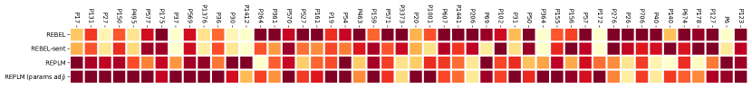
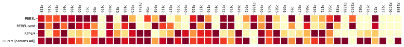
Figure 3: F1 scores per relation type (darker = better). Here, the comparison is made against annotations that additionally make use of external knowledge and should thus more closely reflect the ground-truth. Relation types are arranged in decreasing order of their number of knowledge triplets. For visibility, F1 scores are normalized by the maximum value for each relation.

The above evaluations were constrained by relying solely on the human annotations on DocRED, potentially penalizing accurate methods due to missing annotations. We now repeat our evaluations using an alternative gold standard for a more comprehensive benchmark.

Table 3: Document-level relation extraction results evaluated via external KB. Shown: Micro F1 scores.

Method	F1-Score
REBEL (Cabot et al., 2021)	20.30
REBEL-sent (Cabot et al., 2021)	20.00
REPLM (ours)	32.33
REPLM (params adj) (ours)	36.51
Higher is better. Best value in bold.

Ground-truth via external knowledge: To locate the missing annotations in DocRED, we aggregate all relations extracted from all methods on all documents. We then check the correctness of the extracted relations via an external KB. Specifically, we leverage the pipeline from HELM [33] and check if the generated knowledge triplet exists in Wikidata [67]. We add all the matched triplets to the existing list of ground-truth triplets from DocRED and repeat the evaluation. As a result, total number of relations in the development set increased from 12,212 to 18,592.

Results: For our new dataset with external ground-truth, our framework outperforms REBEL by a considerable margin across most relation types (Fig. 3). This is also seen in the overall performance (Table 3). For example, our REPLM improves the F1 score over REBEL by more than 59 % (32.33 vs. 20.30). The improvement for REPLM (params adj) is even larger and amounts to 80 % (36.51 vs 20.30).

7 Ablation Study: Performance for Sentence-Level Relation Extraction

After showing the effectiveness of our REPLM in document-level relation extraction, we additionally perform sentence-level relation extraction as an ablation study, albeit not our primary benchmarking focus. Despite this, our REPLM still matches or surpasses the performance of fine-tuned LMs.

Datasets. We conduct extensive experiments on three sentence-level relation extraction benchmark datasets, namely CONLL04 [60], NYT [59], and ADE [19]. We provide the details of each dataset in Appendix C.

Baselines. We compare REPLM against fine-tuned LMs that achieve state-of-the-art results: SpERT [13], Table-sequence [73], TANL and TANL (multi-dataset) [51], REBEL (w/o pre-training) and REBEL [7].

Performance. Table 4 shows the micro F1 scores of each method on CONLL04, NYT, and ADE datasets. Our REPLM achieves the best performance on ADE against all the supervised methods with an F1 score of 82.5. We observe that our REPLM performs on par with the state-of-the-art methods on CONLL04 dataset with an F1 score of 72.9, while REBEL attains the best score via an external dataset. For NYT, our REPLM achieves a lower score than state-of-the-art methods. The reason is, the entire NYT is curated via distant supervision, which results in noisy relations. As the baseline methods are fine-tuned with the same dataset, they can memorize the same knowledge triplets from the training set, and therefore, achieve spuriously high performance. The detailed explanation is in Appendix C.

The above analysis also justifies our choice of using REBEL, which is the best of the baselines. It is further the only model that can extract relations from the documents without named entity annotation. Hence, the above ablation also explains why we choose REBEL as the main baseline in Sec. 6.

Table 4: Sentence-level relation extraction. Shown: Micro F1.

Method	CONLL04	NYT	ADE
SpERT [13]	71.5	_	79.2
Table-sequence [73]	73.6	_	80.1
TANL [51]	71.4	90.8	80.6
TANL (multi-dataset) [51]	72.6	90.5	80.0
REBEL (w/o pre-training) (Cabot et al., 2021)	71.2	91.8	81.7
REBEL (Cabot et al., 2021)	75.4	92.0	82.2
REPLM (ours)	72.9	81.0	82.5
Higher is better. Best value in bold.

Further insights. What is the effect of the number of in-context examples? We repeat the same experiment on CONLL04 with a varying number of in-context examples. Fig. 4(a) shows the F1 score on each relation and the overall score by varying $K$ from 3 to 11. We observe that, in general, more in-context examples yield better F1 scores. Informed by this observation, we used the highest number of in-context examples that fit into the context window for our experiments, which is $K=5$ for document-level relation extraction. Detailed results are given in Appendix L.

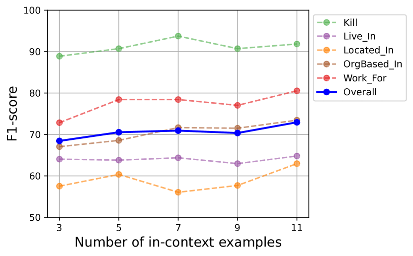
(a) Performance with varying
num. of in-context examples.

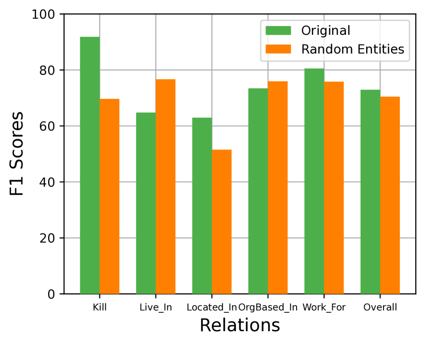
(b) Change in performance with
random entity names.

Figure 4: Ablation studies on CONLL04.

Is REPLM actually learning to extract relations? Or does it only retrieve facts from memory? We design a novel experiment to identify whether our REPLM is learning to extract relations from the input text or it is simply retrieving the facts from its memory. To the best of our knowledge, we are the first to shed more light on the models’ learning ability for the relation extraction task. For this experiment, we replaced all the entities with random names in CONLL04 dataset (for both training and test set) that are not mentioned anywhere in the web. Fig. 4(b) compares the performance against the original dataset. The overall performance decreases only slightly when using the random entities (F1 score of 70.47 vs. 72.9), which is still on par with the state-of-the-art. Therefore, it confirms that our REPLM is an effective method in learning to extract the relations from the context. We provide the experiment details and elaborate on the reasons of slight performance decrease in Appendix M.

8 Discussion

Benefits: Our REPLM framework offers many benefits in practice: (1) REPLM eliminates the need for named entity recognition pipelines in our task and thus the noise that comes with it; (2) REPLM does not require human annotations but leverages in-context few-shot learning; and (3) REPLM offers great flexibility as it allows to incorporate new relations without re-training.

Implications: Our findings have direct implications for constructing datasets and benchmarking methods aimed at relation extraction from the textual documents. Evidently, earlier datasets such as DocRED [86], the largest dataset for document-level relation extraction publicly available, lack comprehensiveness and thus miss important – but correct – annotations. This may penalize correct methods and instead favor overly simple output during benchmarking. Hence, it will be important for future research to develop new datasets and effective evaluation paradigms.

Broader Impact Statement

This paper presents work whose primary goal is to advance the field of machine learning. We would like to emphasize the positive and negative implications that underlie machine learning more broadly. Our REPLM may help to fill the gaps in existing knowledge bases. It is likely that such gaps are particularly dominant for marginalized groups, so that our work can have a positive impact for improving coverage in knowledge bases for diverse groups. Still, LMs are far from perfect as their performance may vary. Hence, careful and responsible use is indicated, especially when filling in knowledge bases with important societal or ethical implications or sensitive content more broadly.

Appendix A Related Work

In-context few-shot learning of LMs: In-context few-shot learning has been widely adopted in text classification tasks [22, 36, 41, 44, 45, 95] and further extended to other tasks such as question answering [22, 36, 45], fact retrieval [95], table-to-text generation [36], and mapping utterances to meaning representations [61]. However, we are not aware of any earlier work that leveraged the in-context few-shot learning paradigm for document-level relation extraction.

LMs as knowledge bases: Research has focused on probing the knowledge in LMs. For example, Petroni et al. [54] introduced the LAMA dataset, a dataset with cloze-style templates for different relations, which allows to probe factual knowledge in LMs. Many works have been introduced to achieve state-of-the-art results via prompt-tuning [21, 30, 32, 38, 39, 48, 53, 55, 63, 97]. Yet, some works further find that, when evaluated as knowledge bases, LMs suffer from inconsistency [2, 15], learn shallow heuristics rather than facts [16], have inferior performance in the long tail [28], and exhibit prompt bias [8].

However, we note that the above research stream is different from our work in two salient ways. (1) In the above research stream, LMs are prompted to retrieve factual knowledge from its memory, whereas we aim to extract the relational knowledge from the context. (2) In the above research stream, LM prompts are structured as “fill-in-the-blank” cloze statement. For example, the task is to output only the correct object, but where both the subject and relation are given. Instead of predicting only the object, our goal is to output the entire knowledge triplet. That is, subject, relation, and object must be inferred together.

Relation extraction via pattern-based and statistical methods: A detailed review of the different methods is provided in Pawar et al. [52] and Weikum et al. [82], while we only present a brief summary here. Early works extracted relations from text via pattern-based extraction methods. Specifically, these works introduced automated methods to extract textual patterns corresponding to each relation and each entity type [9, 27, 47]. Their main limitation is that the automatically constructed patterns involve many mistakes, which, in turn, require human experts to examine and correct them [20].

Another research stream focused on relation extraction via statistical methods. Examples are crafting custom features for relation classification [26, 49], designing customized kernels for support vector machines[49, 74, 91, 90], graphical modeling and inference of relations [62, 87], and leveraging knowledge graph embeddings for relation prediction [35, 77].

However, the above methods have only a limited capacity in capturing complex interactions between entities, as compared to state-of-the-art neural networks [20]. On top of that, both pattern-based and statistical methods require large datasets with human annotation for training.

Relation extraction via neural networks: Initial methods for relation extraction based on neural network approaches made use of convolutional neural network (CNN) [88] and long short-term memory (LSTM) [99] architectures. These works process the pre-computed word embeddings and then classify the relation for the given named entity pair. Follow-up works proposed joint learning of entity extraction and relation classification, again via CNN [1, 96] and LSTM [29, 46] architectures. However, these models are not flexible enough to model the complex interactions between named entities to classify the relation, as compared to LMs.

Relation extraction via LMs: State-of-the-art methods for relation extraction are based on fine-tuning pre-trained LMs. Specifically, these methods use pre-trained LMs such as BERT [12], RoBERTa [40], and SciBERT [4] and fine-tuned them for relation extraction. For instance, Wang et al. [71] fine-tuned BERT to classify the relation between each named entity pair in a given sentence. There have been various follow-up works to improve performance by learning complex dependency between named entities. To achieve this, Wang and Lu [73] jointly trained LSTM and BERT to get two distinct representations of the entities; Zhang et al. [92] further incorporate semantic segmentation module into the fine-tuning of BERT; Zhou et al. [101] propose adaptive thresholding and localized context pooling; Xu et al. [84] explicitly model the dependencies between entity mentions; Paolini et al. [51] augmented the original sentences with the entity and relation types; Tan et al. [65] use axial attention module for learning the interdependency among named entity pairs; Wang Xu and Zhao [78] propose sentence importance estimation; Xiao et al. [83] include additional tasks such as coreference resolution, entity typing, and evidence retrieval; Xu et al. [85] improves the model performance via synthetic data generation; Hu et al. [24] incorporates rationale extraction from the sentence; and Zhang et al. [89] leverages self-distillation to facilitate relational reasoning. However, all of these works require the named entities to be annotated and provided as input at both training and test time.

Appendix B DocRED Dataset

For our experiments, we use DocRED [86], the largest publicly available dataset for document-level relation extraction. We provide the detailed statistics of each relation type in Tables 5 and 6 (note: the different columns compare the different subsets for distant supervision, human-annotated training, and human-annotated dev).

Pre-processing. The original documents in the DocRED dataset are provided only in a tokenized format, e. g., the document is represented as a list of token, where each punctuation mark and word is a different token. We follow the earlier works [7, 86] and concatenate the tokens with a white space in between to construct the entire document. This approach may introduce typos in the documents; for instance, the original text “Tarzan’s Hidden Jungle is a 1955 black-and-white film ...” is reconstructed as “Tarzan ’s Hidden Jungle is a 1955 black - and - white film ...”. We initially tried to fix these typos via spelling correction libraries, such as FastPunct, but later found that the typos are propagated to the labels, which may impede performance and eventually comparability of our results. Therefore, we decided to follow the same pre-processing as earlier works, as it allows us to operate on the same labels as in earlier work and thus ensures comparability of our results. Sec. G shows some examples of documents after the pre-processing step.

Table 5: DocRED statistics

Relation ID	Relation Name	# Docs in Dist. Sup.	# Relations in Dist. Sup.	# Docs in Train	# Relations in Train	# Docs in Dev	# Relations in Dev
P6	head of government	4948	6859	133	210	38	47
P17	country	68402	313961	1831	8921	585	2817
P19	place of birth	21246	31232	453	511	135	146
P20	place of death	15046	24937	170	203	50	52
P22	father	5287	9065	164	273	41	57
P25	mother	1828	2826	50	74	10	15
P26	spouse	4327	9723	134	303	34	74
P27	country of citizenship	45553	126360	1141	2689	384	808
P30	continent	7247	18792	121	356	38	121
P31	instance of	3790	5561	74	103	34	48
P35	head of state	3127	4257	87	140	32	51
P36	capital	27621	34047	66	85	24	27
P37	official language	4040	6562	82	119	29	47
P39	position held	982	1692	15	23	6	8
P40	child	5794	11831	177	360	45	81
P50	author	5265	8856	162	320	49	93
P54	member of sports team	2693	12312	80	379	36	166
P57	director	5891	9865	153	246	58	90
P58	screenwriter	4680	7952	83	156	24	35
P69	educated at	5201	8413	220	316	63	92
P86	composer	2778	4249	44	79	21	57
P102	member of political party	5464	11582	191	406	51	98
P108	employer	4168	6775	126	196	30	54
P112	founded by	5856	7700	74	100	20	27
P118	league	2142	6024	63	185	29	56
P123	publisher	2426	4444	81	172	29	69
P127	owned by	4907	7554	91	208	36	76
P131	located in the administrative territorial entity	44307	143006	1224	4193	389	1227
P136	genre	982	1948	34	111	7	14
P137	operator	1982	3011	52	95	18	41
P140	religion	2515	5143	60	144	26	82
P150	contains administrative territorial entity	34615	62646	1002	2004	310	603
P155	follows	8360	12236	117	188	43	69
P156	followed by	7958	11576	120	192	38	51
P159	headquarters location	12653	17089	206	264	57	86
P161	cast member	6575	21139	163	621	62	226
P162	producer	4434	6739	77	119	32	50
P166	award received	2852	6322	105	173	35	66
P170	creator	3485	6036	96	231	25	40
P171	parent taxon	860	2167	28	75	6	17
P172	ethnic group	6022	7563	63	79	24	30
P175	performer	10783	27945	344	1052	101	332
P176	manufacturer	1260	2737	27	83	9	40
P178	developer	2403	6368	73	238	30	75
P179	series	2404	3800	72	144	27	63
P190	sister city	3388	11471	2	4	1	2
P194	legislative body	2863	2989	136	166	36	56
P205	basin country	2249	3299	61	85	21	32

Table 6: DocRED statistics (continued)

Relation ID	Relation Name	# Docs in Dist. Sup.	# Relations in Dist. Sup.	# Docs in Train	# Relations in Train	# Docs in Dev	# Relations in Dev
P206	located in or next to body of water	3859	6585	109	194	35	83
P241	military branch	1589	2633	69	108	30	42
P264	record label	4524	14804	154	583	49	237
P272	production company	1417	2151	49	82	19	36
P276	location	5281	6654	130	172	55	74
P279	subclass of	1822	2736	39	77	19	36
P355	subsidiary	1761	2436	51	92	18	30
P361	part of	17335	28245	382	596	119	194
P364	original language of work	1061	2274	32	66	11	30
P400	platform	1565	5825	52	304	14	69
P403	mouth of the watercourse	1700	2475	49	95	19	38
P449	original network	2953	4237	97	152	20	39
P463	member of	7364	15272	208	414	55	113
P488	chairperson	1792	2216	49	63	15	21
P495	country of origin	17160	36029	300	539	112	212
P527	has part	13318	22596	317	632	94	177
P551	residence	2629	3197	25	35	5	6
P569	date of birth	26474	33998	893	1044	286	343
P570	date of death	20905	28314	587	805	180	255
P571	inception	19579	26699	393	475	127	154
P576	dissolved, abolished or demolished	5064	7057	52	79	25	39
P577	publication date	17636	37538	576	1142	193	406
P580	start time	5374	6549	96	110	30	32
P582	end time	4943	6144	47	51	18	23
P585	point in time	2457	2920	80	96	29	39
P607	conflict	4119	8056	114	275	46	114
P674	characters	1594	3447	62	163	25	74
P676	lyrics by	1677	2415	30	36	5	8
P706	located on terrain feature	3157	5063	74	137	29	60
P710	participant	2839	4985	95	191	22	57
P737	influenced by	1166	2071	9	9	3	10
P740	location of formation	3885	4531	53	62	12	15
P749	parent organization	2425	3335	47	92	27	40
P800	notable work	4053	5275	102	150	32	56
P807	separated from	1438	2210	2	2	1	2
P840	narrative location	2026	2573	38	48	11	15
P937	work location	5063	7470	69	104	19	22
P1001	applies to jurisdiction	7471	9945	204	298	55	83
P1056	product or material produced	460	624	27	36	6	9
P1198	unemployment rate	1330	1622	2	2	1	1
P1336	territory claimed by	880	1600	18	33	6	10
P1344	participant of	1707	3574	87	223	28	57
P1365	replaces	1490	1811	13	18	9	10
P1366	replaced by	2214	2771	25	36	10	10
P1376	capital of	25241	29816	62	76	20	21
P1412	languages spoken, written or signed	2781	6313	91	155	24	46
P1441	present in work	2872	6763	88	299	34	116
P3373	sibling	3335	11123	102	335	26	134

Appendix C Details on Sentence-Level Relation Extraction

We select three sentence-level relation extraction datasets to show the effectiveness of our REPLM framework against the state-of-the-art supervised methods.

CONLL04 [60] is consisting of sentences collected from the news articles. The authors manually annotated the entities and 5 relation types for each sentence. Following the earlier literature, we used the same splits as Eberts and Ulges [13]. The detailed statistics for each relation type are given in Table 7.

Table 7: CONLL04 statistics

Relation Name	# Sentences in Train	# Relations in Train	# Sentences in Validation	# Relations in Validation	# Sentences in Test	# Relations in Test
Kill	160	179	39	42	46	47
Live_In	270	326	68	84	82	98
Located_In	187	245	52	65	58	90
OrgBased_In	213	260	47	71	70	96
Work_For	208	250	57	69	65	76
Overall	922	1260	231	331	288	407

NYT [59] is composed of sentences from New York Times, containing 24 relation types. The detailed statistics are given in Table 8.

It is important to note that the relations in this dataset are annotated via “distant supervision”, using the knowledge triplets from FreeBase [5]. As a result, the evaluation on the test set becomes noisy. For instance, the sentence in the test set “Mr. Abbas, speaking before a meeting in Paris with the French president, Jacques Chirac, said he was sorry for the shootings on Sunday.” is annotated with the following knowledge triplet “(place of birth, Jacques Chirac, Paris)”, although the birthplace of Jacques Chirac cannot be inferred from the sentence.

We further found that the overlap of relations between train and test set is high. For the relation type place of birth, 166 out of 260 relations (i. e., the exact (relation, subject, object) triplet) in test set appear in the training set. Therefore, although the evaluation on the test is noisy, the baseline methods leverage the supervised training and they can memorize the relations from the train set at the test time. We hypothesize this as the main reason of the inferior performance of our REPLM framework on this dataset specifically, while achieving the state-of-the-art performance at all other evaluations.

Table 8: NYT statistics

Relation Name	# Sentences in Train	# Relations in Train	# Sentences in Validation	# Relations in Validation	# Sentences in Test	# Relations in Test
advisors	37	37	5	5	3	3
capital	6042	6121	557	567	649	659
child	407	437	45	46	32	40
contains_administrative_territorial_entity	4889	5111	462	497	496	527
country	4889	5111	462	497	496	527
country_of_citizenship	6136	6606	545	596	518	548
country_of_origin	19	19	1	1	1	1
denonym	29	32	3	3	1	1
employer	4546	4734	428	448	401	417
ethnicity	19	19	1	1	1	1
founded_by	649	682	53	58	58	61
headquarters_location	180	186	21	22	17	17
industry	1	1	_	_	_	_
location	37626	42961	3302	3818	3296	3835
location_of_formation	344	346	35	35	35	35
major_shareholder	229	238	21	21	31	32
member_of_sports_team	180	186	21	22	17	17
neighborhood_of	4329	4682	403	444	338	374
occupation	2	2	_	_	_	_
place_of_birth	2649	2703	215	217	256	260
place_of_death	1652	1676	125	128	127	131
religion	54	56	7	7	5	5
residence	5883	6182	506	531	570	597
shareholders	229	238	21	21	31	32
Overall	56196	88366	5000	7985	5000	8120

ADE [19] contains the sentences from biomedical domain and it has only one relation type, which is adverse effect. The original dataset contains 10 folds of train and test splits. Following the earlier work [7], we use the test set of the first fold for the evaluation. The statistics are given in Table 9.

Table 9: ADE statistics

Relation Name	# Sentences in Train	# Relations in Train	# Sentences in Validation	# Relations in Validation	# Sentences in Test	# Relations in Test
Adverse-Effect	3845	5980	_	_	427	653

Appendix D In-Context Few-Shot learning based on Distant Supervision vs. Human Annotation

We perform an ablation study to observe the effect of using distantly-supervised vs. human-annotated documents as in-context few-shot examples. We perform such comparison on our four framework variants, namely REPLM (random fixed), REPLM (random all), REPLM (best context$\ominus$), and REPLM (best context$\oplus$). For methods with random in-context examples, the performance may be subject to variability across which seed is picked (whereas the performance is deterministic for the other methods), and, hence, we report the standard deviation for this subset of the methods by averaging the performance across 10 runs. Of note, to directly compare the impact of in-context examples, we deliberately considered our REPLM variants without aggregation over the multiples sets of in-context examples.

Tables 10 to 21 show the comparison between distant supervision vs. human annotation. For random in-context examples (i. e., REPLM (random fixed) and REPLM (random all)), distant supervision and human annotation performs at the same level. For retrieving the semantically most similar context examples (i. e., REPLM (best context$\ominus$) and REPLM (best context$\oplus$)), we observe cases where distant supervision actually improves the result (e. g., P6, P155, P179). However, the overall performance is largely similar. This confirms our choice of using distantly-supervised documents as in-context examples and eliminates the need for human annotation.

Table 10: Ablation study. Comparing the performance across the in-context examples from distant supervision vs. human-annotated train set. Shown are F1 scores on each relation. (Part 1 / 12)

Method	Context Source	P6	P17	P19	P20	P22	P25	P26	P27
REPLM (random fixed)	Train	20.29  $\pm$  8.01	11.18  $\pm$  2.44	75.68  $\pm$  6.45	71.92  $\pm$  4.61	13.17  $\pm$  5.66	0.00  $\pm$  0.00	24.09  $\pm$  5.00	23.03  $\pm$  3.25
REPLM (random fixed)	Dist. Sup.	24.28  $\pm$  10.53	11.34  $\pm$  4.48	66.67  $\pm$  12.71	49.80  $\pm$  16.07	9.76  $\pm$  4.90	0.00  $\pm$  0.00	26.73  $\pm$  4.38	22.41  $\pm$  2.53
REPLM (random all)	Train	19.76  $\pm$  2.59	11.03  $\pm$  0.88	77.17  $\pm$  1.50	68.24  $\pm$  3.54	11.94  $\pm$  3.03	0.00  $\pm$  0.00	24.03  $\pm$  2.73	21.94  $\pm$  1.50
REPLM (random all)	Dist. Sup.	25.90  $\pm$  2.44	11.05  $\pm$  0.46	68.49  $\pm$  3.09	48.35  $\pm$  4.82	9.51  $\pm$  2.86	0.00  $\pm$  0.00	26.74  $\pm$  3.83	23.26  $\pm$  1.39
REPLM (best context$\ominus$)	Train	18.18	19.62	79.29	69.90	15.09	7.14	33.33	28.03
REPLM (best context$\ominus$)	Dist. Sup.	35.96	24.60	71.38	50.39	18.18	15.38	33.33	29.14
REPLM (best context$\oplus$)	Train	18.18	19.65	74.20	72.00	20.00	5.71	30.43	28.27
REPLM (best context$\oplus$)	Dist. Sup.	35.96	24.02	68.63	62.50	17.70	7.41	22.97	28.33

Table 11: Ablation study. Comparing the performance across the in-context examples from distant supervision vs. human-annotated train set. Shown are F1 scores on each relation. (Part 2 / 12)

Method	Context Source	P30	P31	P35	P36	P37	P39	P40	P50
REPLM (random fixed)	Train	16.94  $\pm$  6.32	0.00  $\pm$  0.00	26.86  $\pm$  3.49	16.56  $\pm$  4.57	29.69  $\pm$  10.49	0.00  $\pm$  0.00	15.13  $\pm$  6.04	28.38  $\pm$  4.20
REPLM (random fixed)	Dist. Sup.	13.58  $\pm$  1.66	5.21  $\pm$  2.48	28.79  $\pm$  4.96	18.67  $\pm$  5.96	22.59  $\pm$  8.79	0.00  $\pm$  0.00	12.97  $\pm$  3.62	27.66  $\pm$  4.05
REPLM (random all)	Train	15.43  $\pm$  2.93	6.66  $\pm$  1.82	27.40  $\pm$  3.48	19.92  $\pm$  8.34	27.73  $\pm$  3.60	0.00  $\pm$  0.00	21.05  $\pm$  3.09	28.01  $\pm$  3.89
REPLM (random all)	Dist. Sup.	14.75  $\pm$  2.18	6.33  $\pm$  2.15	26.96  $\pm$  3.17	14.85  $\pm$  5.65	24.13  $\pm$  5.48	0.00  $\pm$  0.00	11.63  $\pm$  3.12	26.74  $\pm$  3.45
REPLM (best context$\ominus$)	Train	19.14	11.90	27.27	22.22	36.36	15.38	29.14	34.18
REPLM (best context$\ominus$)	Dist. Sup.	31.25	6.59	31.46	47.06	31.17	25.00	20.38	38.60
REPLM (best context$\oplus$)	Train	27.84	9.09	21.78	17.54	34.21	0.00	30.87	40.26
REPLM (best context$\oplus$)	Dist. Sup.	30.85	6.82	37.21	45.28	22.78	25.00	26.42	37.66

Table 12: Ablation study. Comparing the performance across the in-context examples from distant supervision vs. human-annotated train set. Shown are F1 scores on each relation. (Part 3 / 12)

Method	Context Source	P54	P57	P58	P69	P86	P102	P108	P112
REPLM (random fixed)	Train	36.25  $\pm$  12.29	30.89  $\pm$  1.64	25.41  $\pm$  5.63	60.96  $\pm$  4.38	17.27  $\pm$  5.49	37.26  $\pm$  5.68	34.50  $\pm$  3.90	24.48  $\pm$  9.40
REPLM (random fixed)	Dist. Sup.	42.71  $\pm$  10.02	34.55  $\pm$  4.59	27.65  $\pm$  6.61	53.00  $\pm$  9.62	16.16  $\pm$  8.57	30.82  $\pm$  9.53	33.29  $\pm$  4.49	14.30  $\pm$  8.81
REPLM (random all)	Train	39.88  $\pm$  6.70	31.76  $\pm$  1.75	27.32  $\pm$  6.41	61.91  $\pm$  2.44	17.29  $\pm$  5.43	32.78  $\pm$  2.11	32.23  $\pm$  2.59	22.26  $\pm$  6.95
REPLM (random all)	Dist. Sup.	43.80  $\pm$  3.48	32.63  $\pm$  3.59	27.32  $\pm$  3.10	57.18  $\pm$  3.74	13.23  $\pm$  4.60	32.85  $\pm$  3.32	32.67  $\pm$  5.06	16.06  $\pm$  6.68
REPLM (best context$\ominus$)	Train	48.67	33.70	35.48	67.07	30.59	37.66	41.38	12.77
REPLM (best context$\ominus$)	Dist. Sup.	48.30	47.62	34.38	57.47	23.26	44.44	30.19	32.65
REPLM (best context$\oplus$)	Train	50.57	40.72	29.41	59.63	35.16	39.74	35.96	17.02
REPLM (best context$\oplus$)	Dist. Sup.	40.93	43.43	39.34	58.29	40.45	40.48	34.29	34.78

Table 13: Ablation study. Comparing the performance across the in-context examples from distant supervision vs. human-annotated train set. Shown are F1 scores on each relation. (Part 4 / 12)

Method	Context Source	P118	P123	P127	P131	P136	P137	P140	P150
REPLM (random fixed)	Train	33.05  $\pm$  6.31	24.29  $\pm$  3.37	10.23  $\pm$  3.89	15.66  $\pm$  2.99	27.79  $\pm$  8.24	14.49  $\pm$  4.58	8.38  $\pm$  3.52	21.52  $\pm$  3.58
REPLM (random fixed)	Dist. Sup.	32.16  $\pm$  5.80	19.81  $\pm$  4.20	11.10  $\pm$  4.41	14.32  $\pm$  2.81	19.70  $\pm$  6.09	9.99  $\pm$  3.84	0.00  $\pm$  0.00	23.36  $\pm$  2.23
REPLM (random all)	Train	32.13  $\pm$  5.64	26.43  $\pm$  3.86	13.17  $\pm$  2.31	15.58  $\pm$  0.62	25.20  $\pm$  7.89	11.77  $\pm$  3.69	6.73  $\pm$  2.76	21.93  $\pm$  1.81
REPLM (random all)	Dist. Sup.	33.51  $\pm$  5.47	19.87  $\pm$  3.15	10.50  $\pm$  3.94	15.54  $\pm$  0.65	21.93  $\pm$  6.65	9.83  $\pm$  2.77	0.00  $\pm$  0.00	21.91  $\pm$  1.52
REPLM (best context$\ominus$)	Train	33.33	20.75	13.79	22.45	22.22	21.18	11.68	0.00
REPLM (best context$\ominus$)	Dist. Sup.	44.04	30.19	18.49	25.50	20.00	12.90	14.17	31.28
REPLM (best context$\oplus$)	Train	36.36	29.41	12.90	22.95	32.00	15.58	9.66	0.00
REPLM (best context$\oplus$)	Dist. Sup.	37.84	19.82	18.03	26.59	26.09	9.84	13.53	30.25

Table 14: Ablation study. Comparing the performance across the in-context examples from distant supervision vs. human-annotated train set. Shown are F1 scores on each relation. (Part 5 / 12)

Method	Context Source	P155	P156	P159	P161	P162	P166	P170	P171
REPLM (random fixed)	Train	5.28  $\pm$  3.31	11.22  $\pm$  5.91	24.25  $\pm$  8.04	27.55  $\pm$  7.43	18.40  $\pm$  7.91	27.09  $\pm$  2.02	5.44  $\pm$  2.44	14.23  $\pm$  3.10
REPLM (random fixed)	Dist. Sup.	6.51  $\pm$  2.64	0.00  $\pm$  0.00	23.72  $\pm$  8.75	30.89  $\pm$  7.21	13.31  $\pm$  4.42	26.45  $\pm$  3.74	6.57  $\pm$  3.01	14.38  $\pm$  6.09
REPLM (random all)	Train	5.45  $\pm$  1.48	11.77  $\pm$  3.67	25.24  $\pm$  2.93	28.60  $\pm$  4.73	20.51  $\pm$  3.65	28.54  $\pm$  2.88	0.00  $\pm$  0.00	13.93  $\pm$  4.04
REPLM (random all)	Dist. Sup.	5.64  $\pm$  1.87	11.47  $\pm$  3.78	23.76  $\pm$  3.43	24.73  $\pm$  4.62	14.47  $\pm$  3.10	24.09  $\pm$  3.17	5.48  $\pm$  2.89	13.65  $\pm$  3.79
REPLM (best context$\ominus$)	Train	0.00	25.81	39.42	36.70	17.20	32.43	13.33	8.00
REPLM (best context$\ominus$)	Dist. Sup.	23.33	21.51	40.85	33.85	14.12	26.92	10.00	10.53
REPLM (best context$\oplus$)	Train	0.00	24.18	39.42	39.63	17.82	38.46	10.67	6.67
REPLM (best context$\oplus$)	Dist. Sup.	22.22	29.21	37.24	30.81	14.81	31.58	11.43	10.53

Table 15: Ablation study. Comparing the performance across the in-context examples from distant supervision vs. human-annotated train set. Shown are F1 scores on each relation. (Part 6 / 12)

Method	Context Source	P172	P175	P176	P178	P179	P190	P194	P205
REPLM (random fixed)	Train	13.59  $\pm$  5.05	36.38  $\pm$  8.61	11.89  $\pm$  5.31	22.27  $\pm$  3.21	14.80  $\pm$  3.95	0.00  $\pm$  0.00	12.67  $\pm$  3.37	20.50  $\pm$  7.77
REPLM (random fixed)	Dist. Sup.	19.33  $\pm$  7.93	34.03  $\pm$  4.85	13.62  $\pm$  4.27	17.96  $\pm$  4.72	10.19  $\pm$  3.41	0.00  $\pm$  0.00	11.62  $\pm$  3.92	16.28  $\pm$  7.56
REPLM (random all)	Train	11.62  $\pm$  3.91	38.49  $\pm$  2.49	12.14  $\pm$  2.80	22.09  $\pm$  2.07	12.95  $\pm$  1.74	0.00  $\pm$  0.00	13.66  $\pm$  4.93	22.61  $\pm$  7.69
REPLM (random all)	Dist. Sup.	16.76  $\pm$  6.25	34.49  $\pm$  2.53	13.54  $\pm$  5.30	21.67  $\pm$  4.32	8.56  $\pm$  2.64	0.00  $\pm$  0.00	13.79  $\pm$  4.14	12.68  $\pm$  4.19
REPLM (best context$\ominus$)	Train	10.91	41.92	22.64	21.62	15.38	66.67	21.51	39.34
REPLM (best context$\ominus$)	Dist. Sup.	23.73	40.71	24.14	28.57	22.45	100.00	19.57	13.56
REPLM (best context$\oplus$)	Train	14.29	43.43	29.09	22.81	17.31	66.67	21.28	22.64
REPLM (best context$\oplus$)	Dist. Sup.	34.48	46.66	23.08	28.99	23.91	66.67	25.81	14.04

Table 16: Ablation study. Comparing the performance across the in-context examples from distant supervision vs. human-annotated train set. Shown are F1 scores on each relation. (Part 7 / 12)

Method	Context Source	P206	P241	P264	P272	P276	P279	P355	P361
REPLM (random fixed)	Train	7.59  $\pm$  3.03	40.15  $\pm$  9.19	35.63  $\pm$  6.93	27.86  $\pm$  5.07	8.40  $\pm$  3.27	0.00  $\pm$  0.00	0.00  $\pm$  0.00	9.31  $\pm$  4.73
REPLM (random fixed)	Dist. Sup.	6.68  $\pm$  3.53	36.97  $\pm$  9.98	28.62  $\pm$  9.75	28.67  $\pm$  3.68	8.32  $\pm$  3.07	0.00  $\pm$  0.00	14.43  $\pm$  6.32	7.36  $\pm$  4.70
REPLM (random all)	Train	5.84  $\pm$  2.03	39.47  $\pm$  3.73	32.63  $\pm$  1.86	26.46  $\pm$  3.73	10.13  $\pm$  2.96	0.00  $\pm$  0.00	15.48  $\pm$  1.86	9.84  $\pm$  1.61
REPLM (random all)	Dist. Sup.	0.00  $\pm$  0.00	33.24  $\pm$  3.41	29.66  $\pm$  2.15	28.10  $\pm$  4.05	9.88  $\pm$  2.77	0.00  $\pm$  0.00	11.26  $\pm$  5.08	7.66  $\pm$  1.82
REPLM (best context$\ominus$)	Train	11.57	46.75	32.29	24.56	17.27	6.56	21.74	18.93
REPLM (best context$\ominus$)	Dist. Sup.	14.63	43.24	30.77	35.09	20.00	11.11	30.77	27.12
REPLM (best context$\oplus$)	Train	8.20	46.58	29.91	21.43	20.44	2.94	17.78	23.10
REPLM (best context$\oplus$)	Dist. Sup.	18.18	45.07	28.35	37.29	22.76	10.91	33.33	25.66

Table 17: Ablation study. Comparing the performance across the in-context examples from distant supervision vs. human-annotated train set. Shown are F1 scores on each relation. (Part 8 / 12)

Method	Context Source	P364	P400	P403	P449	P463	P488	P495	P527
REPLM (random fixed)	Train	24.96  $\pm$  6.35	36.17  $\pm$  10.65	22.47  $\pm$  3.76	29.08  $\pm$  6.31	19.08  $\pm$  2.69	9.85  $\pm$  2.21	15.27  $\pm$  2.74	11.89  $\pm$  2.03
REPLM (random fixed)	Dist. Sup.	22.50  $\pm$  3.05	31.76  $\pm$  10.44	27.58  $\pm$  6.54	20.31  $\pm$  4.25	16.47  $\pm$  5.72	11.17  $\pm$  1.87	12.08  $\pm$  1.52	10.20  $\pm$  2.71
REPLM (random all)	Train	21.75  $\pm$  5.54	41.02  $\pm$  4.49	21.09  $\pm$  3.61	28.86  $\pm$  3.35	16.58  $\pm$  4.92	12.66  $\pm$  4.46	12.95  $\pm$  1.50	10.42  $\pm$  2.31
REPLM (random all)	Dist. Sup.	23.18  $\pm$  5.15	30.09  $\pm$  7.83	27.12  $\pm$  4.96	24.28  $\pm$  5.57	15.54  $\pm$  3.49	10.01  $\pm$  2.80	11.91  $\pm$  2.21	10.55  $\pm$  1.76
REPLM (best context$\ominus$)	Train	35.71	31.37	17.54	30.51	32.09	11.76	18.60	15.95
REPLM (best context$\ominus$)	Dist. Sup.	52.00	40.00	18.52	33.33	38.61	18.18	22.71	23.31
REPLM (best context$\oplus$)	Train	23.26	43.40	14.04	30.51	28.11	11.11	21.05	20.45
REPLM (best context$\oplus$)	Dist. Sup.	43.14	29.36	25.00	27.69	33.80	17.14	21.55	27.63

Table 18: Ablation study. Comparing the performance across the in-context examples from distant supervision vs. human-annotated train set. Shown are F1 scores on each relation. (Part 9 / 12)

Method	Context Source	P551	P569	P570	P571	P576	P577	P580	P582
REPLM (random fixed)	Train	0.00  $\pm$  0.00	54.19  $\pm$  5.75	41.57  $\pm$  3.37	30.85  $\pm$  8.75	7.82  $\pm$  3.26	39.58  $\pm$  4.69	19.20  $\pm$  3.61	24.98  $\pm$  5.96
REPLM (random fixed)	Dist. Sup.	29.09  $\pm$  8.91	51.90  $\pm$  8.21	44.07  $\pm$  3.16	24.60  $\pm$  11.18	8.85  $\pm$  2.46	32.29  $\pm$  5.03	18.35  $\pm$  5.51	0.00  $\pm$  0.00
REPLM (random all)	Train	0.00  $\pm$  0.00	55.28  $\pm$  1.46	42.43  $\pm$  1.70	37.54  $\pm$  2.45	9.69  $\pm$  2.11	36.66  $\pm$  1.80	17.65  $\pm$  4.91	24.41  $\pm$  5.92
REPLM (random all)	Dist. Sup.	0.00  $\pm$  0.00	55.43  $\pm$  1.43	39.35  $\pm$  1.82	23.17  $\pm$  2.44	5.74  $\pm$  2.03	36.61  $\pm$  2.18	19.23  $\pm$  3.65	11.71  $\pm$  4.98
REPLM (best context$\ominus$)	Train	18.18	57.10	44.35	39.73	9.23	43.08	25.81	35.90
REPLM (best context$\ominus$)	Dist. Sup.	36.36	60.95	46.92	38.96	14.49	46.78	27.40	31.11
REPLM (best context$\oplus$)	Train	18.18	56.56	45.55	36.49	5.88	42.28	22.95	34.15
REPLM (best context$\oplus$)	Dist. Sup.	36.36	62.25	46.96	40.27	20.00	45.35	18.46	28.57

Table 19: Ablation study. Comparing the performance across the in-context examples from distant supervision vs. human-annotated train set. Shown are F1 scores on each relation. (Part 10 / 12)

Method	Context Source	P585	P607	P674	P676	P706	P710	P737	P740
REPLM (random fixed)	Train	16.10  $\pm$  4.22	16.02  $\pm$  3.99	25.00  $\pm$  5.89	54.95  $\pm$  6.90	0.00  $\pm$  0.00	8.42  $\pm$  6.01	0.00  $\pm$  0.00	23.41  $\pm$  4.25
REPLM (random fixed)	Dist. Sup.	15.58  $\pm$  4.51	16.23  $\pm$  3.52	23.46  $\pm$  7.00	0.00  $\pm$  0.00	0.00  $\pm$  0.00	6.70  $\pm$  6.66	0.00  $\pm$  0.00	19.36  $\pm$  7.43
REPLM (random all)	Train	18.76  $\pm$  4.51	16.61  $\pm$  1.99	22.46  $\pm$  2.71	58.90  $\pm$  2.15	11.93  $\pm$  2.47	9.23  $\pm$  5.93	0.00  $\pm$  0.00	22.03  $\pm$  8.04
REPLM (random all)	Dist. Sup.	17.37  $\pm$  5.44	15.68  $\pm$  1.45	24.97  $\pm$  4.74	47.97  $\pm$  7.83	6.26  $\pm$  2.60	11.34  $\pm$  2.80	0.00  $\pm$  0.00	20.21  $\pm$  8.17
REPLM (best context$\ominus$)	Train	31.88	17.62	21.43	46.15	13.64	24.49	0.00	23.08
REPLM (best context$\ominus$)	Dist. Sup.	25.64	26.09	26.42	61.54	16.33	27.96	0.00	38.46
REPLM (best context$\oplus$)	Train	35.82	19.79	26.17	61.54	15.05	17.20	0.00	37.04
REPLM (best context$\oplus$)	Dist. Sup.	24.66	26.37	34.29	61.54	12.24	23.40	0.00	37.04

Table 20: Ablation study. Comparing the performance across the in-context examples from distant supervision vs. human-annotated train set. Shown are F1 scores on each relation. (Part 11 / 12)

Method	Context Source	P749	P800	P807	P840	P937	P1001	P1056	P1198
REPLM (random fixed)	Train	11.47  $\pm$  2.41	20.02  $\pm$  4.19	0.00  $\pm$  0.00	35.43  $\pm$  6.25	23.90  $\pm$  4.76	13.51  $\pm$  5.41	0.00  $\pm$  0.00	0.00  $\pm$  0.00
REPLM (random fixed)	Dist. Sup.	10.39  $\pm$  4.08	21.38  $\pm$  2.96	0.00  $\pm$  0.00	26.35  $\pm$  5.02	23.37  $\pm$  6.50	11.84  $\pm$  5.84	0.00  $\pm$  0.00	0.00  $\pm$  0.00
REPLM (random all)	Train	11.32  $\pm$  2.73	20.02  $\pm$  2.55	0.00  $\pm$  0.00	35.41  $\pm$  8.47	22.45  $\pm$  5.03	12.60  $\pm$  1.68	0.00  $\pm$  0.00	0.00  $\pm$  0.00
REPLM (random all)	Dist. Sup.	9.11  $\pm$  4.02	22.51  $\pm$  2.95	0.00  $\pm$  0.00	19.91  $\pm$  3.92	24.87  $\pm$  4.55	11.30  $\pm$  2.91	0.00  $\pm$  0.00	0.00  $\pm$  0.00
REPLM (best context$\ominus$)	Train	22.86	25.64	0.00	30.77	20.51	17.65	14.29	0.00
REPLM (best context$\ominus$)	Dist. Sup.	25.35	31.46	66.67	46.15	21.28	22.06	0.00	100.00
REPLM (best context$\oplus$)	Train	18.46	20.93	0.00	23.08	15.00	21.58	0.00	0.00
REPLM (best context$\oplus$)	Dist. Sup.	25.35	29.27	66.67	46.15	22.22	29.20	0.00	100.00

Table 21: Ablation study. Comparing the performance across the in-context examples from distant supervision vs. human-annotated train set. Shown are F1 scores on each relation. (Part 12 / 12)

Method	Context Source	P1336	P1344	P1365	P1366	P1376	P1412	P1441	P3373
REPLM (random fixed)	Train	0.00  $\pm$  0.00	19.81  $\pm$  7.60	0.00  $\pm$  0.00	0.00  $\pm$  0.00	30.09  $\pm$  7.72	20.64  $\pm$  3.08	16.56  $\pm$  4.57	22.31  $\pm$  5.88
REPLM (random fixed)	Dist. Sup.	0.00  $\pm$  0.00	20.41  $\pm$  6.54	0.00  $\pm$  0.00	0.00  $\pm$  0.00	34.86  $\pm$  10.12	24.65  $\pm$  4.02	15.52  $\pm$  5.30	22.74  $\pm$  5.03
REPLM (random all)	Train	0.00  $\pm$  0.00	18.93  $\pm$  5.08	0.00  $\pm$  0.00	0.00  $\pm$  0.00	32.08  $\pm$  7.43	19.19  $\pm$  2.52	15.38  $\pm$  2.60	21.81  $\pm$  3.52
REPLM (random all)	Dist. Sup.	0.00  $\pm$  0.00	16.99  $\pm$  3.11	0.00  $\pm$  0.00	0.00  $\pm$  0.00	33.58  $\pm$  3.41	25.84  $\pm$  5.77	14.65  $\pm$  4.25	25.44  $\pm$  4.98
REPLM (best context$\ominus$)	Train	0.00	33.33	0.00	0.00	29.27	17.39	16.97	24.04
REPLM (best context$\ominus$)	Dist. Sup.	31.58	45.54	0.00	0.00	52.38	42.35	20.00	20.11
REPLM (best context$\oplus$)	Train	0.00	33.01	0.00	0.00	34.15	33.33	18.60	30.37
REPLM (best context$\oplus$)	Dist. Sup.	31.58	43.40	0.00	0.00	68.29	34.48	29.71	16.48

Appendix E Implementation Details

We provide the details of our REPLM implementation in this section. We use GPT-JT ($\sim$6B parameters) as our pre-trained LM for in-context few-shot learning. As the number of relations to be extracted is unknown in advance, we generate 200 tokens (for comparison, each extracted triplet consumes roughly 10-15 tokens) to ensure that our pre-trained LM can generate all relations it identifies.

As we use a fixed prefix for each extracted knowledge triplet at each line (e. g., “Relation:”), we easily identify if there is no further triplets extracted, simply from the absence of the prefix. We use a special separator token to easily parse the extracted subjects and objects. This separator is “<==>” in our experiments (which cannot be found in the original dataset and therefore cannot be confused with a natural text). We additionally inform our pre-trained LM about the task via starting our prompt with the instruction of the task. Here, we note that we have not done any prompt-tuning, since it is not the focus of this paper. For the output generation, we finally note that we use a greedy-decoding, e. g., not any sampling approach applied, which results in deterministic outputs given the input text. Example inputs and outputs can be found in Sec. G.

In our REPLM framework, we retrieve the semantically most-relevant in-context examples for each dev document. For this, we encode the documents via SBERT [58] to calculate the embeddings and retrieve the most-relevant documents based on the cosine-similarity of the embeddings. We use the following fixed parameters in our framework (if not specified otherwise): $N=20$, $K=5$ $L=5$, $\tau=0.1$, and $\theta=0.2$. As the sentences in sentence-level relation extraction datasets (CONLL04, NYT, and ADE) are shorter than the documents in DocRED, we used more in-context examples for these datasets, which is $K=11$. The other parameters are the same as before.

We run all our experiments on NVIDIA Tesla V100-SXM2 32GB with a batch size 4. For DocRED, on average, each batch is processed in $\sim$17.80 seconds. As a result, the dev set (998 documents) is processed in $\sim$74.17 minutes for each relation type.

Appendix F Empirical Analysis of the Documents that Lack the Annotation

We conjecture that REPLM generates more comprehensive output than REBEL, not because REPLM the probability threshold $\theta$ is too low but because REPLM identifies annotations that are missing in the dataset. To validate this empirically, we thus adopt a simple yet effective strategy to predict if a given document contains information about the given relation. Fig. 5 plots the average cosine similarity between (i)  documents in the dev split and (ii) their top-$N$ nearest neighbors in distantly-supervised documents. The histogram shows two modes in distribution, where one corresponds to “known” relation and one to “missing” relations. In the overlap of two distributions, there are semantically similar documents that potentially include the relation but lack the annotation.

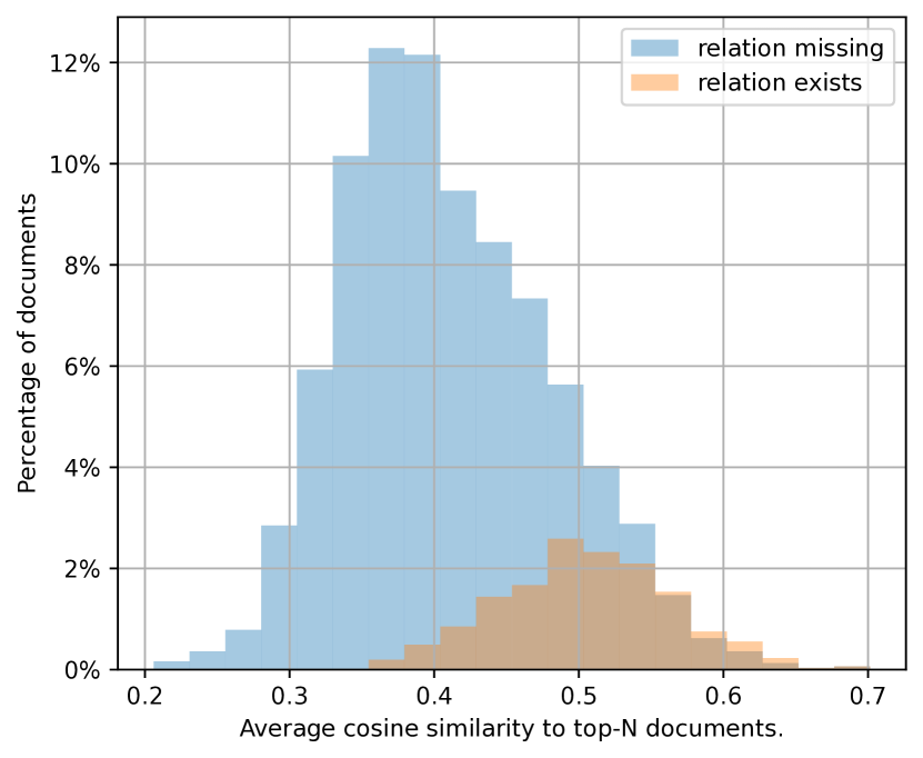
(a) P19

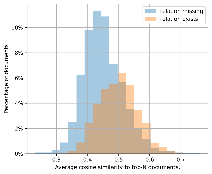
(b) P27

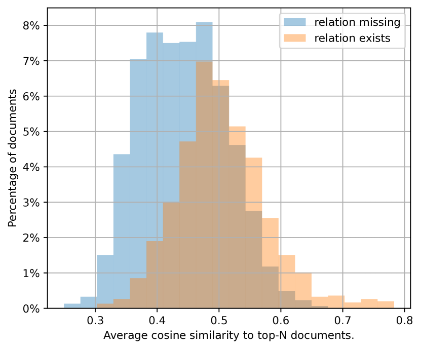
(c) P131

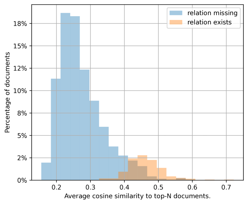
(d) P175

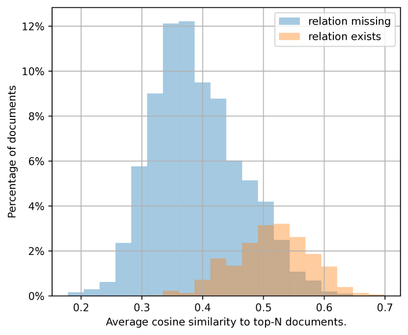
(e) P570

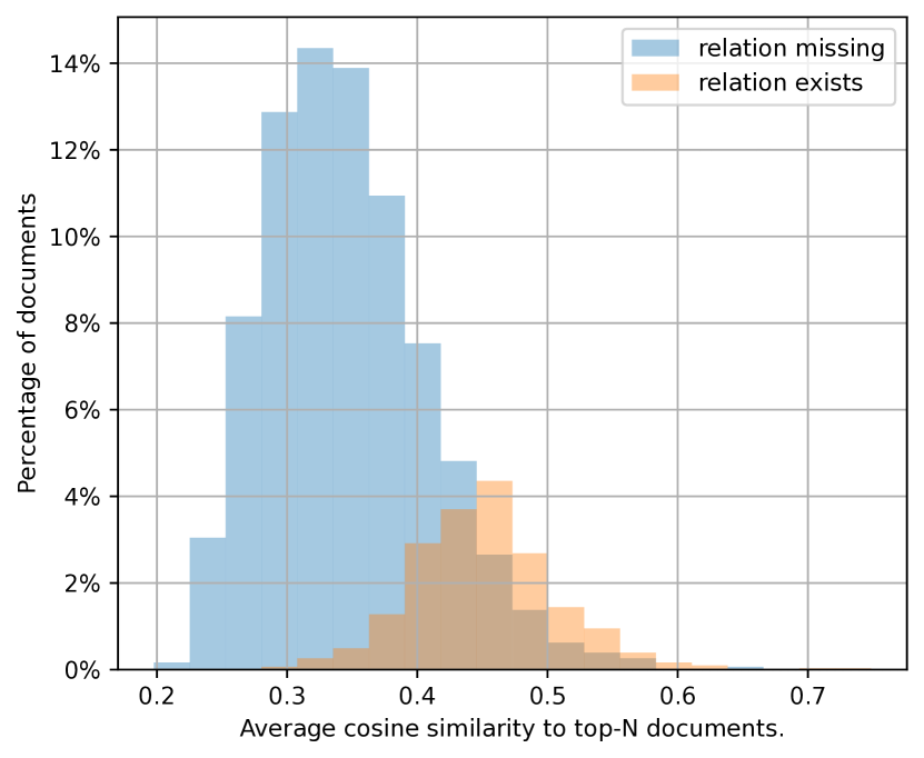
(f) P577

Figure 5: Histogram of average cosine similarity between documents and their top-$N$ neighbors for two example relation types.

Appendix G Example Prompts and Outputs

In the following, we provide examples for different prompts as input (in red) and the corresponding output (in blue).

G.1 P17 (country)

Input Prompt:

Your task is to identify all the unique knowledge triplets of ’country’ for a given context. Knowledge triplet will be ordered as relation, subject, and object, which are separated by <==>. If there are multiple triplets, list each of them in a new line. Follow the example context-relation pairs for the formatting of your output.

Context: IBM Laboratory Vienna was an IBM research laboratory based in Vienna , Austria . The laboratory started with a group led by Heinz Zemanek that moved from the Technische Hochschule ( now the Technical University of Vienna ) . Initially , the group worked on computer hardware projects . Later a compiler for the ALGOL 60 programming language was produced . The group built on ideas of Calvin C. Elgot , Peter Landin , and John McCarthy , to create an operational semantics that could define the whole of IBM ’s PL / I programming language . The meta - language used for this was dubbed by people outside the laboratory as the Vienna Definition Language ( VDL ) . These descriptions were used for compiler design research into compiler design during 1968 - 70 . The formal method VDM ( Vienna Development Method ) was a result of research at the laboratory by Dines Bjørner , Cliff Jones , Peter Lucas , and others .

Relation: (country <==> Vienna <==> Austria)

Relation: (country <==> Technical University of Vienna <==> Austria)

Context: The School of Engineering of Juiz de Fora ( ) was an engineering college in the city of Juiz de Fora , Brazil . It is now the engineering faculty of the Federal University of Juiz de Fora ( UFJF ) . The former president of Brazil Itamar Franco was an alumnus . It was set up in 1914 in the city of Juiz de Fora , Minas Gerais state , Brazil , and taught a five - year course of Civil and Eletrotechnic Engineering . In 1960 , the school joined the Medicine , Pharmacy and Law schools of that city to found the UFJF . Nowadays , the Faculty of Engineering provides courses in civil , production , electrical ( divided into telecommunication , energy , power , electronic , robotic and automation systems ) , mechanical , computer , sanitary and environmental engineering , and architecture . Relation: (country <==> School of Engineering of Juiz de Fora <==> Brazil)

Relation: (country <==> Juiz de Fora <==> Brazil)

Relation: (country <==> UFJF <==> Brazil)

Relation: (country <==> Minas Gerais <==> Brazil)

Context: Bizrate Insights Inc. , doing business as Bizrate Insights , is a market research company , providing consumer ratings information to over 6,000 retailers and publishers across the United States , United Kingdom , France , Germany , and Canada . Bizrate Insights is a Meredith Corporation company based in Los Angeles , CA . Bizrate Insights provides services to both businesses and consumers in two different ways : consumers have access to ratings and reviews from verified buyers that help to inform their purchase decisions . This feedback can be found on the Bizrate website and is syndicated across the web to major search engines such as Google and Bing . Bizrate Insights provides businesses with customer satisfaction insights about consumers , advanced analytics , and competitive benchmarks across all types of online retail industries . Bizrate Insights also provides industry research to analysts at Forrester Research and Internet Retailer for publication and studies . Relation: (country <==> Meredith Corporation <==> the United States)

Relation: (country <==> Los Angeles <==> the United States)

Relation: (country <==> Google <==> the United States)

Relation: (country <==> Bing <==> the United States)

Context: The Universidade Positivo ( abbreviated UP ) is a private universities of the State of Paraná , Brazil . Universidade Positivo ’s campus is in the Campo Comprido district of Curitiba and occupies an area of 420,004 m2 . Its 114,000 m2 of installations . Universidade Positivo currently offers 27 undergraduate programs , a doctoral program , three master ’s degree programs , certificate of graduate study programs and extension courses . The 6,300 m2 library can hold 864 users at a time . Its collection consists of nearly 115,000 volumes . In a special room the library houses the personal collection of the late cabinet minister , diplomat and professor , Roberto de Oliveira Campos . It includes diplomas , medals and awards , in addition to its 8,426 volumes .

Relation: (country <==> Universidade Positivo <==> Brazil)

Relation: (country <==> State of Paraná <==> Brazil)

Relation: (country <==> Curitiba <==> Brazil)

Context: Softtek is a Mexican - based information technology company , operating in North America , Latin America , Europe and Asia . As of 2010 it was the largest private IT vendor in Latin America . Headquartered in Monterrey , Mexico , the company has 12,000 associates in Mexico and abroad . The company offers application software development , testing , security and support ; business process outsourcing ( BPO ) ; and IT infrastructure management , security and support to more than 400 corporations in more than 20 countries . It also acts as a value added reseller ( VAR ) for SAP SE , Informatica , Cognos , Business Objects and other software products . The company has trademarked the term " nearshoring " to describe the provision of outsourced services to customers in other countries that are in proximity .

Relation: (country <==> Softtek <==> Mexico)

Relation: (country <==> Monterrey <==> Mexico)

Context: IBM Research – Brazil is one of twelve research laboratories comprising IBM Research , its first in South America . It was established in June 2010 , with locations in São Paulo and Rio de Janeiro . Research focuses on Industrial Technology and Science , Systems of Engagement and Insight , Social Data Analytics and Natural Resources Solutions . The new lab , IBM ’s ninth at the time of opening and first in 12 years , underscores the growing importance of emerging markets and the globalization of innovation . In collaboration with Brazil ’s government , it will help IBM to develop technology systems around natural resource development and large - scale events such as the 2016 Summer Olympics . Engineer and associate lab director Ulisses Mello explains that IBM has four priority areas in Brazil : " The main area is related to natural resources management , involving oil and gas , mining and agricultural sectors . The second is the social data analytics segment that comprises the analysis of data generated from social networking sites [ such as Twitter or Facebook ] , which can be applied , for example , to financial analysis . The third strategic area is nanotechnology applied to the development of the smarter devices for the intermittent production industry . This technology can be applied to , for example , blood testing or recovering oil from existing fields . And the last one is smarter cities .

Output:

Relation: (country <==> IBM Research – Brazil <==> Brazil)

Relation: (country <==> São Paulo <==> Brazil)

Relation: (country <==> Rio de Janeiro <==> Brazil)

Relation: (country <==> 2016 Summer Olympics <==> Brazil)

Relation: (country <==> Industrial Technology and Science <==> Brazil)

Correctness:

For relation P17 (country), the given dev document is annotated with two knowledge triplets (country, São Paulo, Brazil) and (country, Rio de Janeiro, Brazil). For this document, we find that the annotators did not consider the country information of the event “2016 Summer Olympics” and the organization “IBM Research – Brazil” for their manual annotation. Validating from an external knowledge base, we observe that our REPLM framework identifies two more knowledge triplets correctly, (country, 2016 Summer Olympics, Brazil) and (country, Industrial Technology and Science, Brazil).

G.2 P118 (league)

Input Prompt:

Your task is to identify all the unique knowledge triplets of ’league’ for a given context. Knowledge triplet will be ordered as relation, subject, and object, which are separated by <==>. If there are multiple triplets, list each of them in a new line. Follow the example context-relation pairs for the formatting of your output.

Context: Richard Ian Wright ( born 5 November 1977 ) is an English retired professional footballer who played as a goalkeeper . He currently works as a coach for Manchester City . Born in Ipswich , he joined Ipswich Town as a trainee , going on to play for the club 298 times between 1995 and 2001 . He then moved to Premier League club Arsenal , before being signed by Everton in 2002 , where he spent five years . A brief spell on loan from West Ham United with Southampton was followed by a transfer back to Ipswich Town . After a short spell at Sheffield United , a third stint at Ipswich and a brief time at Preston North End , he joined Premier League champions Manchester City on a free transfer in 2012 . After four years at City , during which he did not play at all , he announced his retirement in May 2016 . He remained with City as a coach under new manager Pep Guardiola . He was a member of the England squad , earning two caps , and was included in their squad for UEFA Euro 2000 .

Relation: (league <==> Manchester City <==> Premier League)

Relation: (league <==> Arsenal <==> Premier League)

Relation: (league <==> Everton <==> Premier League)

Relation: (league <==> West Ham United <==> Premier League)

Relation: (league <==> Southampton <==> Premier League)

Context: Ashley Renaldo Chambers ( born 1 March 1990 ) is an English professional footballer who plays as a winger or a striker for club Kidderminster Harriers . Chambers started his career with Leicester City , making his first - team debut in 2005 at the age of 15 in a League Cup match against Blackpool , which made him the youngest player in the club ’s history . In 2009 , he joined League One club Wycombe Wanderers on loan . This was followed by a loan period with League Two club Grimsby Town . He signed for Conference Premier club York City on loan in November 2010 before signing permanently . He won in the 2012 FA Trophy Final and 2012 Conference Premier play - off Final with York at Wembley Stadium , the latter seeing the club promoted into League Two . Chambers joined Conference Premier club Cambridge United in 2014 .

Relation: (league <==> Kidderminster Harriers <==> Conference Premier)

Relation: (league <==> Leicester City <==> League One)

Context: Roy Eric Carroll ( born 30 September 1977 ) is a Northern Irish professional footballer who plays as a goalkeeper for NIFL Premiership side Linfield . He is best known for his spells at Wigan Athletic , Manchester United ( where he won a Premier League winners medal and the 2004 FA Cup ) and Olympiacos ( where he won the Greek Superleague three times and the Greek Cup twice ) . He has also represented Northern Ireland 45 times at full international level , gaining his first cap in 1997 , aged 19 . Carroll has also had a one - game managerial career , leading Barnet to a 2 - 1 victory in the 2011 Herts Senior Cup final against Stevenage . Therefore , Carroll holds the unusual honour of having won a trophy in his only game as a manager .

Relation: (league <==> Linfield <==> NIFL Premiership)

Relation: (league <==> Manchester United <==> Premier League)

Relation: (league <==> Olympiacos <==> Greek Superleague)

Context: Brian Christopher Deane ( born 7 February 1968 ) is an English football coach and former player whose most recent position was as the manager of the Norwegian side Sarpsborg 08 . During his playing career , he played as forward from 1985 until 2006 . He was the scorer of the first ever goal in the FA Premier League in 1992 , when he was a Sheffield United player . Deane also played in the Premier League for Leeds United and Middlesbrough as well as playing top - flight football in Portugal and Australia for Benfica and Perth Glory respectively . He also played in The Football League for Doncaster Rovers , Leicester City , West Ham United and Sunderland before finishing his playing career in 2006 with a brief spell back at Sheffield United . Deane was capped three times by England .

Relation: (league <==> Middlesbrough <==> FA Premier League)

Relation: (league <==> Leicester City <==> FA Premier League)

Relation: (league <==> West Ham United <==> FA Premier League)

Context: John Stones ( born 28 May 1994 ) is an English professional footballer who plays for club Manchester City and the English national team . Mainly a centre back , he can also play as a right back . Stones began his career with Barnsley , making his first - team debut in the Championship in March 2012 as a 17-year - old . He joined Premier League club Everton for around £ 3 million in January 2013 and amassed 95 appearances over four seasons . In August 2016 , he signed for Manchester City for an initial £ 47.5 million with add - ons . He won the Premier League and EFL Cup in 2018 . Stones made his senior debut for England in May 2014 after previously being capped by England youth teams at under-19 , under-20 and under-21 levels . He was chosen in England ’s squads for UEFA Euro 2016 and the 2018 FIFA World Cup .

Relation: (league <==> Manchester City <==> Premier League)

Relation: (league <==> Manchester City <==> EFL Cup)

Relation: (league <==> Barnsley <==> Championship)

Relation: (league <==> Everton <==> Premier League)

Context: Andrew Alexander Cole ( born 15 October 1971 ) is an English former professional footballer . Playing as a striker , his career lasted from 1988 to 2008 . He is most notably remembered for his time in the Premier League , with Manchester United , where he spent six years of his career , winning numerous trophies in the process . He also played in the top division of English football for Arsenal , Newcastle United , Blackburn Rovers , Fulham , Manchester City , Portsmouth and Sunderland , as well as in the Football League for Bristol City , Birmingham City , Burnley and Nottingham Forest . He is the third - highest goalscorer in Premier League history with 187 goals . Cole has the distinction of being one of the few players in England to have swept all possible honours in the English game , including the PFA Young Player of the Year award , as well as the coveted UEFA Champions League title . Cole was also capped 15 times for the England national team between 1995 and 2001 , scoring once against Albania in a 2002 FIFA World Cup qualifier .

Output:

Relation: (league <==> Manchester United <==> Premier League)

Relation: (league <==> Newcastle United <==> Premier League)

Relation: (league <==> Blackburn Rovers <==> Premier League)

Relation: (league <==> Fulham <==> Premier League)

Relation: (league <==> Manchester City <==> Premier League)

Relation: (league <==> Portsmouth <==> Premier League)

Relation: (league <==> Sunderland <==> Premier League)

Correctness:

For relation P118 (league), the given dev document is annotated with only one knowledge triplet (league, Manchester United, Premier League). In this example, our pre-trained LM identifies 6 more knowledge triplets via in-context few-shot learning. At the time of writing, the following triplets are also correct (league, Newcastle United, Premier League), (league, Fulham, Premier League), (league, Manchester City, Premier League). We note that although such information is outdated, Blackburn Rovers, Portsmouth, and Sunderland can be inferred as in Premier League from the same passage. This also highlights the need that the relation extraction methods should additionally infer (if possible) for which time period the extracted information is valid.

G.3 P272 (production company)

Input Prompt:

Your task is to identify all the unique knowledge triplets of ’production company’ for a given context. Knowledge triplet will be ordered as relation, subject, and object, which are separated by <==>. If there are multiple triplets, list each of them in a new line. Follow the example context-relation pairs for the formatting of your output.

Context: Ron Moody ( born Ronald Moodnick , 8 January 1924 - 11 June 2015 ) was an English actor , singer , composer and writer best known for his portrayal of Fagin in Oliver ! ( 1968 ) and its 1983 Broadway revival . Moody earned a Golden Globe Award and an Academy Award nomination for the film , as well as a Tony Award nomination for the stage production . Other notable projects include The Mouse on the Moon ( 1963 ) , Mel Brooks ’ The Twelve Chairs ( 1970 ) and Flight of the Doves ( 1971 ) , in which Moody shared the screen with Oliver ! co - star Jack Wild . Moody holds the peculiar distinction of having portrayed the wizard Merlin in two Disney films , Unidentified Flying Oddball ( 1979 ) and A Kid in King Arthur ’s Court ( 1995 ) .

Relation: (production company <==> Unidentified Flying Oddball <==> Disney)

Context: The Beastmaster is a 1982 sword and sorcery film directed by Don Coscarelli and starring Marc Singer , Tanya Roberts , John Amos and Rip Torn loosely based on the novel The Beast Master by Andre Norton . The film is about a child who is stolen from his mother ’s womb by a witch . The child grows into Dar , who has the ability to communicate telepathically with animals . Dar grows up in a village where he learns to do battle . But the village is destroyed by a race of beast - like warriors under the control of the sorcerer Maax . Dar vows revenge and travels with new friends to stop Maax from causing any more problems . Commercially The Beastmaster was not considered a box office success during its original cinematic run ; however later it received extensive television exposure and success on cable in the American market on channels TBS and HBO . The original film spawned two sequels as well as a syndicated television series that chronicled the further adventures of Dar .

Relation: (production company <==> Beastmaster <==> Don Coscarelli)

Context: Monkeybone is a 2001 American black comedy dark fantasy film directed by Henry Selick , written by Sam Hamm , and produced by Selick , Hamm , Mark Radcliffe , Michael Barnathan , and Chris Columbus . The film combines live - action with stop - motion animation . Based on Kaja Blackley ’s graphic novel Dark Town , the film stars an ensemble cast led by Brendan Fraser , Bridget Fonda , and Whoopi Goldberg with Rose McGowan , Dave Foley , Giancarlo Esposito , Megan Mullally , Lisa Zane , Chris Kattan , John Turturro , and an uncredited Thomas Haden Church . Theatrically released on February 23 , 2001 by 20th Century Fox , the film was a box office bomb and received generally negative critical reviews .

Relation: (production company <==> Monkeybone <==> 20th Century Fox)

Context: TaleSpin is an American animated television series based in the fictional city of Cape Suzette , that first aired in 1990 as a preview on The Disney Channel and later that year as part of The Disney Afternoon , with characters adapted from Disney ’s 1967 animated feature The Jungle Book , which was theatrically rereleased in the summer before this show premiered in the fall . The name of the show is a play on tailspin , the rapid descent of an aircraft in a steep spiral . The two words in the show ’s name , tale and spin , are a way to describe telling a story . The show is one of ten Disney Afternoon shows to use established Disney characters as the main characters , with the others being Darkwing Duck , DuckTales , Chip ’ n Dale Rescue Rangers , Goof Troop , Bonkers , Quack Pack , Aladdin , Timon & Pumbaa and Jungle Cubs . It is also one of the two animated television series based on The Jungle Book along with Jungle Cubs .

Relation: (production company <==> Aladdin <==> Disney)

Context: Tarzan ’s Hidden Jungle is a 1955 black - and - white film from RKO Pictures directed by Harold D. Schuster and starring Gordon Scott in his first film as Tarzan , taking over the role from Lex Barker , who had in turn followed Johnny Weissmuller in the series . The film about Edgar Rice Burroughs ’ ape - man also features Vera Miles and Jack Elam . It was the last of twelve Tarzan pictures released by RKO . Tarzan ’s mate , Jane , does not appear in the film . Tarzan at first seems to show more than casual interest in Miles ’ character , but ultimately there is no romance . In real life , Scott and Miles were married after the film was completed . Scott eventually played Tarzan in six movies over a five - year span .

Relation: (production company <==> Tarzan ’s Hidden Jungle <==> RKO Pictures)

Context: King Louie is a fictional character introduced in Walt Disney ’s 1967 animated musical film , The Jungle Book . Unlike the majority of the adapted characters in the film , Louie was not featured in Rudyard Kipling ’s original works . King Louie was portrayed as an orangutan who was the leader of the other jungle primates , and who attempted to gain knowledge of fire from Mowgli , in order to become more human . King Louie was voiced by Louis Prima in the original 1967 film . Initially , the filmmakers considered Louis Armstrong for the role , but to avoid the likely controversy that would result from casting a black person to voice an ape , they instead chose Prima , a white singer . Christopher Walken voiced King Louie in the 2016 live - action / CGI The Jungle Book film .

Output:

Relation: (production company <==> The Jungle Book <==> Walt Disney)

Correctness:

For relation P637 (production company), there was no annotation for the given dev document. However, our framework identifies the knowledge triplet (production company, The Jungle Book, Walt Disney). This can easily be inferred from the first sentence of the document.

Appendix H Full Results on Overall Performance

Tables 22 to 33 provide the detailed results of relation extraction of all methods on all relation types. For methods with random in-context examples, the performance may be subject to variability across which seed is picked (whereas the performance is deterministic for the other methods), and, hence, we report the standard deviation for this subset of the methods by averaging the performance across 10 runs. The evaluation is done based on the human annotations of the dev documents.

When we compare the different variants of our framework, the results confirm our choice in the complete REPLM framework. Specifically, we find that (1) retrieving the best in-context examples improves the performance compared to random examples (i. e., REPLM (best context$\ominus$) and REPLM (best context$\oplus$) vs. REPLM (random fixed) and REPLM (random all)) and (2) our complete REPLM framework brings a significant improvement over REPLM (best context$\ominus$) and REPLM (best context$\oplus$) by aggregating multiple sets of most relevant in-context examples, thus establishing the importance of using multiple sets. We further compare our framework against the state-of-the-art relation extraction method REBEL and find that, overall, our REPLM and REPLM (params adj) perform the best.

Table 22: Full results in overall performance (Section 6.1). Shown are F1 scores on each relation. (Part 1 / 12)

Method	P6	P17	P19	P20	P22	P25	P26	P27
REBEL	0.00	20.66	50.89	29.41	40.86	38.10	41.32	5.69
REBEL-sent	4.08	25.73	45.95	29.85	33.71	30.00	41.84	11.37
REPLM (random fixed)	24.28  $\pm$  10.53	11.34  $\pm$  4.48	66.67  $\pm$  12.71	49.80  $\pm$  16.07	9.76  $\pm$  4.90	0.00  $\pm$  0.00	26.73  $\pm$  4.38	22.41  $\pm$  2.53
REPLM (random all)	25.90  $\pm$  2.44	11.05  $\pm$  0.46	68.49  $\pm$  3.09	48.35  $\pm$  4.82	9.51  $\pm$  2.86	0.00  $\pm$  0.00	26.74  $\pm$  3.83	23.26  $\pm$  1.39
REPLM (best context$\ominus$)	35.96	24.60	71.38	50.39	18.18	15.38	33.33	29.14
REPLM (best context$\oplus$)	35.96	24.02	68.63	62.50	17.70	7.41	22.97	28.33
REPLM	34.78	27.74	59.06	40.41	17.17	28.00	37.17	30.71
REPLM (params adj)	29.79	27.85	77.49	59.77	15.54	22.54	40.24	34.64

Table 23: Full results in overall performance (Section 6.1). Shown are F1 scores on each relation. (Part 2 / 12)

Method	P30	P31	P35	P36	P37	P39	P40	P50
REBEL	6.40	9.84	0.00	57.89	0.00	46.15	39.02	42.76
REBEL-sent	10.29	16.16	3.70	55.81	0.00	33.33	35.00	51.81
REPLM (random fixed)	13.58  $\pm$  1.66	5.21  $\pm$  2.48	28.79  $\pm$  4.96	18.67  $\pm$  5.96	22.59  $\pm$  8.79	0.00  $\pm$  0.00	12.97  $\pm$  3.62	27.66  $\pm$  4.05
REPLM (random all)	14.75  $\pm$  2.18	6.33  $\pm$  2.15	26.96  $\pm$  3.17	14.85  $\pm$  5.65	24.13  $\pm$  5.48	0.00  $\pm$  0.00	11.63  $\pm$  3.12	26.74  $\pm$  3.45
REPLM (best context$\ominus$)	31.25	6.59	31.46	47.06	31.17	25.00	20.38	38.60
REPLM (best context$\oplus$)	30.85	6.82	37.21	45.28	22.78	25.00	26.42	37.66
REPLM	39.11	14.29	32.56	52.46	27.91	8.70	17.56	41.12
REPLM (params adj)	38.94	14.04	29.58	52.83	29.73	12.50	20.38	41.12

Table 24: Full results in overall performance (Section 6.1). Shown are F1 scores on each relation. (Part 3 / 12)

Method	P54	P57	P58	P69	P86	P102	P108	P112
REBEL	38.06	48.53	19.05	41.38	26.67	49.32	26.87	27.78
REBEL-sent	25.22	40.60	5.26	5.31	16.90	60.61	26.09	20.51
REPLM (random fixed)	42.71  $\pm$  10.02	34.55  $\pm$  4.59	27.65  $\pm$  6.61	53.00  $\pm$  9.62	16.16  $\pm$  8.57	30.82  $\pm$  9.53	33.29  $\pm$  4.49	14.30  $\pm$  8.81
REPLM (random all)	43.80  $\pm$  3.48	32.63  $\pm$  3.59	27.32  $\pm$  3.10	57.18  $\pm$  3.74	13.23  $\pm$  4.60	32.85  $\pm$  3.32	32.67  $\pm$  5.06	16.06  $\pm$  6.68
REPLM (best context$\ominus$)	48.30	47.62	34.38	57.47	23.26	44.44	30.19	32.65
REPLM (best context$\oplus$)	40.93	43.43	39.34	58.29	40.45	40.48	34.29	34.78
REPLM	45.78	43.70	30.77	56.25	51.33	42.26	31.88	31.43
REPLM (params adj)	43.42	45.99	35.82	64.41	51.33	45.90	34.00	37.21

Table 25: Full results in overall performance (Section 6.1). Shown are F1 scores on each relation. (Part 4 / 12)

Method	P118	P123	P127	P131	P136	P137	P140	P150
REBEL	34.21	27.59	13.48	31.01	19.05	16.67	4.65	33.49
REBEL-sent	40.74	30.11	18.69	28.61	16.67	8.16	14.81	39.53
REPLM (random fixed)	32.16  $\pm$  5.80	19.81  $\pm$  4.20	11.10  $\pm$  4.41	14.32  $\pm$  2.81	19.70  $\pm$  6.09	9.99  $\pm$  3.84	0.00  $\pm$  0.00	23.36  $\pm$  2.23
REPLM (random all)	33.51  $\pm$  5.47	19.87  $\pm$  3.15	10.50  $\pm$  3.94	15.54  $\pm$  0.65	21.93  $\pm$  6.65	9.83  $\pm$  2.77	0.00  $\pm$  0.00	21.91  $\pm$  1.52
REPLM (best context$\ominus$)	44.04	30.19	18.49	25.50	20.00	12.90	14.17	31.28
REPLM (best context$\oplus$)	37.84	19.82	18.03	26.59	26.09	9.84	13.53	30.25
REPLM	39.75	32.47	21.52	29.89	18.18	17.72	14.29	34.36
REPLM (params adj)	46.28	35.77	21.79	29.79	18.18	17.95	14.55	33.75

Table 26: Full results in overall performance (Section 6.1). Shown are F1 scores on each relation. (Part 5 / 12)

Method	P155	P156	P159	P161	P162	P166	P170	P171
REBEL	2.70	7.02	22.02	37.96	10.91	28.92	28.07	16.00
REBEL-sent	16.33	24.39	35.90	17.74	7.27	38.64	31.58	13.79
REPLM (random fixed)	6.51  $\pm$  2.64	0.00  $\pm$  0.00	23.72  $\pm$  8.75	30.89  $\pm$  7.21	13.31  $\pm$  4.42	26.45  $\pm$  3.74	6.57  $\pm$  3.01	14.38  $\pm$  6.09
REPLM (random all)	5.64  $\pm$  1.87	11.47  $\pm$  3.78	23.76  $\pm$  3.43	24.73  $\pm$  4.62	14.47  $\pm$  3.10	24.09  $\pm$  3.17	5.48  $\pm$  2.89	13.65  $\pm$  3.79
REPLM (best context$\ominus$)	23.33	21.51	40.85	33.85	14.12	26.92	10.00	10.53
REPLM (best context$\oplus$)	22.22	29.21	37.24	30.81	14.81	31.58	11.43	10.53
REPLM	16.09	29.93	45.03	45.23	23.81	26.42	15.52	14.63
REPLM (params adj)	16.47	30.07	42.11	46.21	23.64	27.59	17.50	10.81

Table 27: Full results in overall performance (Section 6.1). Shown are F1 scores on each relation. (Part 6 / 12)

Method	P172	P175	P176	P178	P179	P190	P194	P205
REBEL	0.00	47.90	13.04	28.32	0.00	0.00	10.00	11.76
REBEL-sent	0.00	45.88	32.79	28.04	0.00	0.00	17.39	16.22
REPLM (random fixed)	19.33  $\pm$  7.93	34.03  $\pm$  4.85	13.62  $\pm$  4.27	17.96  $\pm$  4.72	10.19  $\pm$  3.41	0.00  $\pm$  0.00	11.62  $\pm$  3.92	16.28  $\pm$  7.56
REPLM (random all)	16.76  $\pm$  6.25	34.49  $\pm$  2.53	13.54  $\pm$  5.30	21.67  $\pm$  4.32	8.56  $\pm$  2.64	0.00  $\pm$  0.00	13.79  $\pm$  4.14	12.68  $\pm$  4.19
REPLM (best context$\ominus$)	23.73	40.71	24.14	28.57	22.45	100.00	19.57	13.56
REPLM (best context$\oplus$)	34.48	46.66	23.08	28.99	23.91	66.67	25.81	14.04
REPLM	32.91	52.19	28.17	31.75	27.27	66.67	30.65	25.35
REPLM (params adj)	30.77	53.27	29.73	31.75	23.30	66.67	21.51	27.12

Table 28: Full results in overall performance (Section 6.1). Shown are F1 scores on each relation. (Part 7 / 12)

Method	P206	P241	P264	P272	P276	P279	P355	P361
REBEL	34.11	26.42	42.61	44.90	19.05	4.55	6.06	37.45
REBEL-sent	31.25	12.24	27.39	48.00	26.42	15.15	23.53	26.09
REPLM (random fixed)	6.68  $\pm$  3.53	36.97  $\pm$  9.98	28.62  $\pm$  9.75	28.67  $\pm$  3.68	8.32  $\pm$  3.07	0.00  $\pm$  0.00	14.43  $\pm$  6.32	7.36  $\pm$  4.70
REPLM (random all)	0.00  $\pm$  0.00	33.24  $\pm$  3.41	29.66  $\pm$  2.15	28.10  $\pm$  4.05	9.88  $\pm$  2.77	0.00  $\pm$  0.00	11.26  $\pm$  5.08	7.66  $\pm$  1.82
REPLM (best context$\ominus$)	14.63	43.24	30.77	35.09	20.00	11.11	30.77	27.12
REPLM (best context$\oplus$)	18.18	45.07	28.35	37.29	22.76	10.91	33.33	25.66
REPLM	20.51	46.00	45.54	36.36	30.12	9.09	22.22	25.39
REPLM (params adj)	11.57	53.12	46.75	36.36	32.79	8.96	28.07	25.33

Table 29: Full results in overall performance (Section 6.1). Shown are F1 scores on each relation. (Part 8 / 12)

Method	P364	P400	P403	P449	P463	P488	P495	P527
REBEL	0.00	36.54	38.46	0.00	43.90	17.39	3.54	37.04
REBEL-sent	0.00	36.17	44.12	0.00	40.23	8.33	5.69	34.45
REPLM (random fixed)	22.50  $\pm$  3.05	31.76  $\pm$  10.44	27.58  $\pm$  6.54	20.31  $\pm$  4.25	16.47  $\pm$  5.72	11.17  $\pm$  1.87	12.08  $\pm$  1.52	10.20  $\pm$  2.71
REPLM (random all)	23.18  $\pm$  5.15	30.09  $\pm$  7.83	27.12  $\pm$  4.96	24.28  $\pm$  5.57	15.54  $\pm$  3.49	10.01  $\pm$  2.80	11.91  $\pm$  2.21	10.55  $\pm$  1.76
REPLM (best context$\ominus$)	52.00	40.00	18.52	33.33	38.61	18.18	22.71	23.31
REPLM (best context$\oplus$)	43.14	29.36	25.00	27.69	33.80	17.14	21.55	27.63
REPLM	39.34	34.01	27.03	38.10	42.07	14.81	22.41	21.74
REPLM (params adj)	38.10	35.21	21.28	39.39	41.05	20.00	21.82	23.49

Table 30: Full results in overall performance (Section 6.1). Shown are F1 scores on each relation. (Part 9 / 12)

Method	P551	P569	P570	P571	P576	P577	P580	P582
REBEL	0.00	50.51	39.19	50.93	0.00	35.32	21.05	0.00
REBEL-sent	25.00	51.32	44.44	42.59	0.00	42.79	23.81	0.00
REPLM (random fixed)	29.09  $\pm$  8.91	51.90  $\pm$  8.21	44.07  $\pm$  3.16	24.60  $\pm$  11.18	8.85  $\pm$  2.46	32.29  $\pm$  5.03	18.35  $\pm$  5.51	0.00  $\pm$  0.00
REPLM (random all)	0.00  $\pm$  0.00	55.43  $\pm$  1.43	39.35  $\pm$  1.82	23.17  $\pm$  2.44	5.74  $\pm$  2.03	36.61  $\pm$  2.18	19.23  $\pm$  3.65	11.71  $\pm$  4.98
REPLM (best context$\ominus$)	36.36	60.95	46.92	38.96	14.49	46.78	27.40	31.11
REPLM (best context$\oplus$)	36.36	62.25	46.96	40.27	20.00	45.35	18.46	28.57
REPLM	28.57	55.73	44.56	39.71	17.78	52.39	29.17	43.14
REPLM (params adj)	33.33	61.29	50.66	46.78	19.35	54.40	35.48	46.15

Table 31: Full results in overall performance (Section 6.1). Shown are F1 scores on each relation. (Part 10 / 12)

Method	P585	P607	P674	P676	P706	P710	P737	P740
REBEL	11.32	42.17	28.26	0.00	5.88	25.32	0.00	12.50
REBEL-sent	28.57	38.64	21.15	0.00	2.94	20.22	0.00	10.53
REPLM (random fixed)	15.58  $\pm$  4.51	16.23  $\pm$  3.52	23.46  $\pm$  7.00	0.00  $\pm$  0.00	0.00  $\pm$  0.00	6.70  $\pm$  6.66	0.00  $\pm$  0.00	19.36  $\pm$  7.43
REPLM (random all)	17.37  $\pm$  5.44	15.68  $\pm$  1.45	24.97  $\pm$  4.74	47.97  $\pm$  7.83	6.26  $\pm$  2.60	11.34  $\pm$  2.80	0.00  $\pm$  0.00	20.21  $\pm$  8.17
REPLM (best context$\ominus$)	25.64	26.09	26.42	61.54	16.33	27.96	0.00	38.46
REPLM (best context$\oplus$)	24.66	26.37	34.29	61.54	12.24	23.40	0.00	37.04
REPLM	30.11	33.20	31.25	47.06	23.02	30.19	0.00	31.58
REPLM (params adj)	28.26	27.69	23.30	46.15	17.39	23.66	0.00	31.25

Table 32: Full results in overall performance (Section 6.1). Shown are F1 scores on each relation. (Part 11 / 12)

Method	P749	P800	P807	P840	P937	P1001	P1056	P1198
REBEL	4.26	39.47	0.00	0.00	0.00	15.05	0.00	0.00
REBEL-sent	32.35	43.90	0.00	0.00	0.00	1.94	0.00	0.00
REPLM (random fixed)	10.39  $\pm$  4.08	21.38  $\pm$  2.96	0.00  $\pm$  0.00	26.35  $\pm$  5.02	23.37  $\pm$  6.50	11.84  $\pm$  5.84	0.00  $\pm$  0.00	0.00  $\pm$  0.00
REPLM (random all)	9.11  $\pm$  4.02	22.51  $\pm$  2.95	0.00  $\pm$  0.00	19.91  $\pm$  3.92	24.87  $\pm$  4.55	11.30  $\pm$  2.91	0.00  $\pm$  0.00	0.00  $\pm$  0.00
REPLM (best context$\ominus$)	25.35	31.46	66.67	46.15	21.28	22.06	0.00	100.00
REPLM (best context$\oplus$)	25.35	29.27	66.67	46.15	22.22	29.20	0.00	100.00
REPLM	24.49	29.27	50.00	34.29	28.57	28.57	0.00	100.00
REPLM (params adj)	21.05	32.56	50.00	30.77	21.74	28.57	0.00	66.67

Table 33: Full results in overall performance (Section 6.1). Shown are F1 scores on each relation. (Part 12 / 12)

Method	P1336	P1344	P1365	P1366	P1376	P1412	P1441	P3373
REBEL	0.00	0.00	18.18	18.18	25.00	0.00	27.78	41.81
REBEL-sent	0.00	0.00	33.33	23.53	24.00	0.00	18.54	46.35
REPLM (random fixed)	0.00  $\pm$  0.00	20.41  $\pm$  6.54	0.00  $\pm$  0.00	0.00  $\pm$  0.00	34.86  $\pm$  10.12	24.65  $\pm$  4.02	15.52  $\pm$  5.30	22.74  $\pm$  5.03
REPLM (random all)	0.00  $\pm$  0.00	16.99  $\pm$  3.11	0.00  $\pm$  0.00	0.00  $\pm$  0.00	33.58  $\pm$  3.41	25.84  $\pm$  5.77	14.65  $\pm$  4.25	25.44  $\pm$  4.98
REPLM (best context$\ominus$)	31.58	45.54	0.00	0.00	52.38	42.35	20.00	20.11
REPLM (best context$\oplus$)	31.58	43.40	0.00	0.00	68.29	34.48	29.71	16.48
REPLM	26.09	35.80	0.00	0.00	55.17	28.81	30.15	28.22
REPLM (params adj)	26.09	35.58	0.00	0.00	60.87	28.81	30.61	29.27

Appendix I Full Results on Comparison Against External Knowledge

Tables 34 to 41 provide the detailed results of relation extraction of all methods on all relation types. The evaluation is done based on checking the correctness of extracted relations against both the human annotations of the dev documents and an external knowledge base.

Overall, we see that our our REPLM and REPLM (params adj) outperforms REBEL in most relations, when further including the relations from an external knowledge base. The performance improvement becomes more striking for the relation types having a large number of knowledge triplets. For instance, for the relation P17 (country), our REPLM achieves an F1 score of 56.14, whereas REBEL-sent can achieve less than the half of the performance, F1 score of 21.17. We want to highlight that, these methods performed at similar level when compared against only human-annotations as ground-truth (REPLM with 27.74 F1 score vs. REBEL-sent with 25.73 F1 score, see Sec. H). Therefore, it shows the importance of evaluating against an external knowledge base. Even a larger performance gap can be found in relation P27 (country of citizenship), our REPLM and REPLM (params adj) achieve the F1 scores 39.52 and 46.15, respectively, whereas REBEL and REBEL-sent can achieve only F1 scores 3.47 and 8.24. These results further confirm the effectiveness of our REPLM framework, agreeing with the results from the earlier sections.

Table 34: Full results in comparison against external knowledge (Section 6.2). Shown are F1 scores on each relation. (Part 1 / 8)

Method	P6	P17	P19	P20	P22	P25	P26	P27	P30	P31	P35	P36
REBEL	0.00	17.08	37.46	13.92	35.09	30.77	35.86	3.47	3.22	4.80	0.00	15.34
REBEL-sent	2.13	21.17	34.55	14.29	27.74	26.32	30.66	7.72	8.24	2.81	2.78	16.90
REPLM	14.81	56.14	33.83	10.90	3.86	9.16	6.40	39.52	49.16	9.78	5.85	14.63
REPLM (params adj)	14.04	55.32	53.67	37.84	12.68	10.31	4.08	46.15	39.22	13.89	13.86	26.94

Table 35: Full results in comparison against external knowledge (Section 6.2). Shown are F1 scores on each relation. (Part 2 / 8)

Method	P37	P39	P40	P50	P54	P57	P58	P69	P86	P102	P108	P112
REBEL	0.00	30.11	34.97	43.27	37.84	48.05	16.90	35.79	31.25	47.13	27.91	15.38
REBEL-sent	0.00	13.39	28.07	40.89	24.00	41.56	2.82	5.23	15.38	57.58	20.00	10.31
REPLM	8.79	2.50	2.75	14.15	45.04	38.82	24.78	37.76	19.48	37.04	6.01	3.12
REPLM (params adj)	18.60	15.00	4.97	30.84	45.04	38.32	25.23	35.23	25.64	37.78	22.22	12.96

Table 36: Full results in comparison against external knowledge (Section 6.2). Shown are F1 scores on each relation. (Part 3 / 8)

Method	P118	P123	P127	P131	P136	P137	P140	P150	P155	P156	P159	P161
REBEL	29.09	26.67	12.28	28.54	4.29	12.50	4.12	29.01	6.67	8.06	13.86	42.52
REBEL-sent	36.99	23.44	12.31	26.03	2.37	5.06	12.70	33.80	7.91	12.31	21.67	21.20
REPLM	34.55	25.24	6.61	38.54	19.40	9.09	0.00	43.21	9.52	4.88	21.88	24.62
REPLM (params adj)	33.63	26.92	11.03	42.39	13.33	9.52	8.55	47.81	10.98	11.70	23.85	32.56

Table 37: Full results in comparison against external knowledge (Section 6.2). Shown are F1 scores on each relation. (Part 4 / 8)

Method	P162	P166	P170	P171	P172	P175	P176	P178	P179	P190	P194	P205
REBEL	10.20	31.37	25.00	10.81	0.00	49.91	15.62	30.43	0.00	0.00	9.09	5.56
REBEL-sent	6.38	36.21	24.44	6.45	0.00	46.49	32.18	32.06	0.00	0.00	14.14	15.58
REPLM	11.04	5.94	6.90	27.91	12.28	42.04	24.76	1.06	0.62	6.85	9.30	12.50
REPLM (params adj)	10.48	26.79	10.34	26.32	21.97	42.16	24.72	16.36	19.51	6.18	14.43	14.46

Table 38: Full results in comparison against external knowledge (Section 6.2). Shown are F1 scores on each relation. (Part 5 / 8)

Method	P206	P241	P264	P272	P276	P279	P355	P361	P364	P400	P403	P449
REBEL	28.88	27.59	44.39	38.71	18.03	5.00	10.67	27.42	0.00	37.38	36.11	0.00
REBEL-sent	24.91	12.90	27.37	40.58	18.00	2.28	14.37	12.41	0.00	34.00	36.89	0.00
REPLM	4.41	3.96	0.00	4.61	9.01	19.72	6.90	16.35	16.25	32.18	23.73	48.65
REPLM (params adj)	4.32	58.97	29.06	27.35	9.35	15.24	9.52	13.30	37.91	32.18	23.08	44.44

Table 39: Full results in comparison against external knowledge (Section 6.2). Shown are F1 scores on each relation. (Part 6 / 8)

Method	P463	P488	P495	P527	P551	P569	P570	P571	P576	P577	P580	P582
REBEL	32.03	15.38	3.47	29.70	7.14	50.08	38.79	44.90	0.00	34.01	19.51	0.00
REBEL-sent	24.58	5.88	4.50	16.55	10.81	50.82	43.56	27.59	0.00	39.40	14.71	0.00
REPLM	9.33	0.00	12.52	8.43	5.56	57.76	38.81	29.67	0.97	21.96	6.90	0.86
REPLM (params adj)	15.92	16.95	19.80	20.00	5.00	62.15	46.31	31.20	4.00	42.14	7.48	5.61

Table 40: Full results in comparison against external knowledge (Section 6.2). Shown are F1 scores on each relation. (Part 7 / 8)

Method	P585	P607	P674	P676	P706	P710	P737	P740	P749	P800	P807	P840
REBEL	5.50	38.78	25.64	0.00	11.43	16.53	0.00	11.76	5.26	29.31	0.00	0.00
REBEL-sent	3.35	34.36	19.86	0.00	8.62	13.79	0.00	12.90	14.77	24.71	0.00	0.00
REPLM	21.43	26.14	18.02	3.62	7.62	2.55	0.00	25.93	0.00	8.89	2.98	3.95
REPLM (params adj)	20.00	24.86	15.24	14.71	7.62	26.67	6.67	27.40	6.32	17.35	15.24	4.94

Table 41: Full results in comparison against external knowledge (Section 6.2). Shown are F1 scores on each relation. (Part 8 / 8)

Method	P937	P1001	P1056	P1198	P1336	P1344	P1365	P1366	P1376	P1412	P1441	P3373
REBEL	0.00	11.03	0.00	0.00	0.00	0.00	6.25	3.70	7.06	0.00	28.07	39.58
REBEL-sent	7.06	3.37	0.00	0.00	0.00	0.00	10.81	4.12	4.61	0.00	19.29	32.93
REPLM	4.42	12.56	0.00	0.00	0.00	49.52	0.00	0.00	36.36	34.22	15.71	7.41
REPLM (params adj)	12.35	17.83	0.00	1.19	13.95	47.27	0.00	0.00	37.85	12.03	15.83	8.78

Appendix J Sensitivity Analysis of our REPLM Framework

In our original REPLM framework, we used a fixed temperature $\tau$ and a fixed probability threshold $\theta$ as our REPLM does not require a human-annotated training documents to tune the hyperparameters. Tables 42 to 47 show the sensitivity of REPLM on various hyperparameter selections for all relation types individually. Overall, we observe that our REPLM framework is robust to different hyperparameter: the performance remains at the same level for most variations. (Only exception is $\theta=0.5$, where such high probability threshold results in discarding the correctly extracted relations. This leads to much lower recall, and therefore, F1 score.) This also explains why the performance gap between REPLM and REPLM (params adj) is small.

Table 42: Sensitivity of our REPLM framework predictions w.r.t $\tau$ and $\theta$. Shown are F1 scores on each relation. (Part 1 / 6)

$\tau$	$\theta$	P6	P17	P19	P20	P22	P25	P26	P27	P30	P31	P35	P36	P37	P39	P40	P50
0.01	0.01	33.11	25.88	57.28	41.05	16.11	22.58	35.96	29.08	36.69	11.51	30.88	45.95	22.22	8.70	17.87	40.00
0.01	0.05	34.07	26.13	60.31	43.43	17.30	20.83	36.89	30.39	38.43	12.61	29.03	51.61	27.37	9.52	16.22	42.05
0.01	0.10	36.67	25.36	64.09	47.50	12.82	14.63	36.27	31.77	32.69	12.77	32.73	53.33	30.95	0.00	16.67	38.67
0.01	0.20	40.40	24.55	71.03	54.96	12.60	20.00	38.32	32.39	31.46	14.63	34.69	48.00	27.40	0.00	16.18	37.50
0.01	0.50	24.62	17.25	76.26	57.78	14.12	10.00	35.48	25.56	26.49	12.70	30.14	42.86	10.91	0.00	17.09	33.57
0.05	0.01	31.06	25.78	55.94	40.20	17.65	22.54	36.89	28.29	33.87	10.39	29.17	45.00	21.85	7.14	17.09	41.41
0.05	0.05	31.25	26.86	56.34	40.20	17.94	22.95	36.51	28.81	38.20	11.94	29.37	46.58	25.00	8.33	17.65	40.00
0.05	0.10	35.56	27.63	60.10	41.05	15.54	28.00	38.01	30.75	39.46	14.16	33.33	52.46	27.91	9.09	17.83	41.18
0.05	0.20	32.65	26.12	69.91	52.24	20.80	16.67	40.24	34.45	34.09	15.58	36.00	52.83	29.73	12.50	17.75	41.98
0.05	0.50	16.95	13.68	77.94	57.47	13.33	11.11	31.78	24.81	22.07	7.02	31.43	46.15	11.32	0.00	12.24	33.59
0.10	0.01	31.06	25.75	55.94	40.20	17.65	22.54	36.89	28.29	33.65	10.32	29.17	45.00	21.85	7.14	17.03	41.41
0.10	0.05	31.25	26.85	56.34	40.20	17.47	22.22	37.04	28.68	36.36	11.76	29.58	45.95	25.24	8.00	17.59	41.78
0.10	0.10	32.99	26.16	70.34	53.03	19.83	16.67	40.25	34.65	34.48	15.79	35.05	52.83	29.73	12.50	18.63	41.25
0.10	0.20	34.78	27.74	59.06	40.41	17.17	28.00	37.17	30.71	39.11	14.29	32.56	52.46	27.91	8.70	17.56	41.12
0.10	0.50	16.95	13.63	77.49	58.14	13.33	11.11	32.08	24.84	22.07	7.02	30.99	46.15	11.32	0.00	10.31	33.59
0.20	0.01	31.06	25.72	55.94	40.20	17.65	22.54	36.89	28.29	33.65	10.32	29.17	45.00	21.85	7.14	17.03	41.41
0.20	0.05	31.25	26.78	56.21	40.20	18.26	22.22	37.19	28.66	34.91	11.76	29.58	45.33	25.24	8.00	17.53	41.59
0.20	0.10	34.53	27.68	59.20	40.41	18.00	28.00	37.00	30.56	38.94	14.29	31.82	51.61	28.24	9.09	17.16	43.52
0.20	0.20	33.33	26.39	70.99	53.12	18.64	11.43	41.56	34.56	34.48	16.00	35.42	52.83	30.14	13.33	20.13	41.51
0.20	0.50	20.00	13.71	77.49	58.14	13.33	11.11	33.64	24.86	20.83	7.02	30.99	46.15	11.32	0.00	10.20	33.59
0.50	0.01	31.06	25.73	55.94	40.20	17.65	22.54	36.89	28.28	33.65	10.32	29.17	45.00	21.85	7.14	17.03	41.41
0.50	0.05	31.25	26.73	56.21	40.20	18.26	22.58	37.19	28.65	34.78	11.76	29.58	45.95	25.49	8.00	17.53	41.59
0.50	0.10	34.04	27.77	59.35	40.21	17.91	28.00	37.00	30.54	38.94	14.04	31.58	51.61	27.91	9.09	17.23	43.12
0.50	0.20	29.79	26.23	70.99	53.97	18.49	11.43	39.74	34.55	33.33	15.79	35.42	52.83	30.14	13.33	20.25	41.77
0.50	0.50	20.00	13.96	77.49	59.77	13.33	11.11	33.64	24.98	20.83	7.02	23.19	46.15	11.32	0.00	10.20	33.59
1.00	0.01	31.06	25.73	55.94	40.20	17.65	22.54	36.89	28.28	33.65	10.32	29.17	45.00	21.85	7.14	17.03	41.41
1.00	0.05	31.25	26.73	56.21	40.20	18.26	22.22	37.19	28.65	34.91	11.76	29.58	45.95	25.24	8.00	17.53	41.59
1.00	0.10	33.09	27.85	59.35	40.21	18.72	28.00	37.00	30.54	38.77	14.04	31.34	51.61	27.91	9.09	17.10	43.12
1.00	0.20	29.79	26.18	71.21	53.97	18.80	11.43	39.74	34.64	33.33	15.79	35.42	52.83	30.56	13.33	20.38	41.77
1.00	0.50	20.00	13.97	77.49	59.77	13.33	11.11	32.08	24.81	20.83	7.02	23.19	46.15	11.32	0.00	10.20	33.59

Table 43: Sensitivity of our REPLM framework predictions w.r.t $\tau$ and $\theta$. Shown are F1 scores on each relation. (Part 2 / 6)

$\tau$	$\theta$	P54	P57	P58	P69	P86	P102	P108	P112	P118	P123	P127	P131	P136	P137	P140	P150
0.01	0.01	44.71	42.55	30.00	56.39	52.54	39.43	29.73	30.14	35.16	32.47	19.28	29.07	21.05	15.38	16.17	32.25
0.01	0.05	45.26	43.17	31.58	60.29	50.45	38.71	31.34	28.57	39.47	32.17	20.13	28.64	25.81	17.95	15.03	32.92
0.01	0.10	42.81	43.48	33.33	58.59	49.06	42.92	31.15	33.33	40.88	31.34	20.00	27.52	20.69	13.51	13.70	34.45
0.01	0.20	39.86	45.41	35.82	59.67	39.58	45.60	31.48	35.56	42.28	29.75	19.67	24.54	17.39	16.13	13.79	33.10
0.01	0.50	41.53	47.20	37.93	61.44	19.18	41.77	27.78	36.84	37.65	30.43	18.56	15.82	11.11	8.16	6.38	24.12
0.05	0.01	43.06	42.28	29.63	56.77	52.54	39.04	30.07	26.83	34.97	32.34	19.69	28.97	24.39	14.00	15.44	32.13
0.05	0.05	44.06	42.98	29.63	56.77	52.54	39.72	30.46	29.33	35.96	31.90	20.11	29.35	27.03	14.58	15.02	32.86
0.05	0.10	45.45	44.44	31.58	55.86	51.79	41.38	31.65	31.25	40.25	32.65	22.08	30.02	18.75	17.95	14.55	34.27
0.05	0.20	43.42	47.42	35.82	64.41	38.71	46.07	34.00	40.91	45.90	35.20	20.87	26.60	16.00	17.54	13.45	33.77
0.05	0.50	35.71	48.05	38.60	60.00	17.14	35.71	25.71	24.24	37.04	30.23	17.78	13.51	12.50	4.35	4.55	20.25
0.10	0.01	43.06	42.28	29.63	56.77	52.54	39.04	30.07	26.51	34.97	32.34	19.59	28.95	24.39	14.00	15.50	32.11
0.10	0.05	43.68	42.98	29.63	56.77	52.54	39.86	30.46	28.57	35.96	32.73	20.65	29.39	27.03	14.43	14.88	32.72
0.10	0.10	43.42	47.12	36.36	64.74	38.71	45.90	35.42	37.21	46.28	35.77	22.41	26.68	16.67	17.24	13.68	33.74
0.10	0.20	45.78	43.70	30.77	56.25	51.33	42.26	31.88	31.43	39.75	32.47	21.52	29.89	18.18	17.72	14.29	34.36
0.10	0.50	36.28	47.06	39.29	59.06	17.14	36.23	25.71	24.24	37.04	30.59	19.78	13.55	12.50	4.35	4.60	20.08
0.20	0.01	43.06	42.28	29.63	56.77	52.54	39.04	30.07	26.51	34.97	32.34	19.59	28.95	24.39	14.00	15.44	32.11
0.20	0.05	43.68	42.80	29.63	56.77	52.54	39.86	30.46	28.57	35.96	32.53	20.54	29.27	27.03	14.58	14.75	32.77
0.20	0.10	45.78	43.51	30.38	56.25	49.12	42.38	32.17	31.43	39.75	33.99	21.79	30.07	18.75	17.72	13.25	34.15
0.20	0.20	43.42	45.74	36.92	65.12	35.16	43.43	36.56	37.21	47.06	37.61	22.61	26.65	17.39	17.24	13.68	34.10
0.20	0.50	35.96	47.06	40.74	58.11	17.14	36.50	25.71	24.24	39.02	30.59	20.00	13.31	12.50	4.44	4.60	19.58
0.50	0.01	43.06	42.28	29.63	56.77	52.54	39.04	30.07	26.51	34.97	32.34	19.59	28.95	24.39	14.00	15.44	32.11
0.50	0.05	43.68	42.62	29.63	56.77	52.54	39.58	30.46	28.57	35.96	32.53	20.54	29.29	27.03	14.58	14.75	32.73
0.50	0.10	45.65	43.15	30.38	56.50	47.79	42.07	32.17	31.43	39.51	33.99	21.79	29.89	24.24	17.50	13.10	33.90
0.50	0.20	44.04	45.99	36.92	65.12	35.56	43.43	34.78	37.21	47.46	36.84	23.01	26.47	16.67	17.54	13.56	34.02
0.50	0.50	35.96	48.05	40.74	58.11	17.14	36.50	25.71	29.41	39.02	30.59	20.00	13.32	12.50	4.44	4.60	19.89
1.00	0.01	43.06	42.28	29.63	56.77	52.54	39.04	30.07	26.19	34.97	32.34	19.59	28.95	24.39	14.00	15.44	32.11
1.00	0.05	43.68	42.62	29.63	56.77	52.54	39.58	30.46	28.57	35.96	32.53	20.54	29.30	27.03	14.58	14.61	32.71
1.00	0.10	45.51	43.15	30.38	57.14	47.79	42.07	32.17	31.43	39.26	33.99	21.79	29.79	24.24	17.50	13.10	33.92
1.00	0.20	44.20	45.99	36.92	65.50	35.56	42.53	34.78	37.21	47.46	36.84	23.21	26.37	16.67	17.54	13.56	33.75
1.00	0.50	35.96	48.05	40.74	58.11	17.14	35.29	25.71	29.41	39.02	30.59	20.00	13.32	12.50	8.70	4.60	19.89

Table 44: Sensitivity of our REPLM framework predictions w.r.t $\tau$ and $\theta$. Shown are F1 scores on each relation. (Part 3 / 6)

$\tau$	$\theta$	P155	P156	P159	P161	P162	P166	P170	P171	P172	P175	P176	P178	P179	P190	P194	P205
0.01	0.01	15.84	26.44	41.58	45.04	24.06	27.50	16.81	14.63	31.37	50.90	27.03	32.51	25.00	66.67	26.21	23.38
0.01	0.05	15.57	28.17	44.09	46.60	24.59	27.40	17.48	10.81	35.44	51.75	28.57	32.46	27.64	66.67	27.87	24.62
0.01	0.10	17.39	26.23	43.68	45.96	23.64	27.48	14.74	11.43	37.68	52.24	28.99	31.82	26.55	66.67	25.69	27.12
0.01	0.20	13.79	27.08	43.87	43.17	16.28	30.36	13.33	12.12	30.51	50.17	25.00	32.26	26.42	66.67	24.74	24.49
0.01	0.50	14.12	24.24	35.59	35.53	8.96	30.77	11.76	14.81	26.09	43.15	9.09	19.64	23.26	66.67	17.39	5.13
0.05	0.01	14.29	25.26	39.09	43.73	24.64	26.51	17.14	14.63	28.32	49.94	28.57	31.78	24.83	66.67	24.20	23.53
0.05	0.05	14.29	26.82	40.76	44.18	24.82	27.16	18.18	14.63	31.58	50.86	28.95	32.23	25.00	66.67	25.50	25.32
0.05	0.10	16.47	31.21	46.24	46.21	24.00	27.27	14.55	14.63	32.91	51.99	28.17	31.02	26.98	66.67	29.27	23.88
0.05	0.20	11.97	27.66	44.30	47.86	26.37	34.23	17.72	11.43	30.77	53.27	34.48	32.89	22.43	66.67	21.51	16.00
0.05	0.50	14.81	22.58	35.09	36.80	9.38	27.59	8.16	15.38	15.00	39.39	4.76	18.37	20.25	66.67	12.70	5.26
0.10	0.01	14.29	25.26	39.09	43.73	24.64	26.51	17.14	14.63	28.32	49.94	28.57	31.78	24.83	66.67	24.20	23.53
0.10	0.05	14.08	26.52	40.57	44.03	24.82	27.16	17.52	14.63	30.30	50.55	28.95	31.92	24.83	66.67	25.50	25.00
0.10	0.10	12.28	27.37	42.31	47.95	27.59	34.55	17.50	11.43	29.63	53.00	31.58	32.43	23.30	66.67	23.91	16.33
0.10	0.20	16.09	29.93	45.03	45.23	23.81	26.42	15.52	14.63	32.91	52.19	28.17	31.75	27.27	66.67	30.65	25.35
0.10	0.50	14.81	19.67	37.93	36.90	9.38	27.59	12.50	16.00	10.26	38.94	9.30	19.57	20.00	66.67	15.62	5.13
0.20	0.01	14.29	25.26	39.09	43.73	24.64	26.35	17.14	14.63	28.32	49.94	28.57	31.78	24.83	66.67	24.20	23.53
0.20	0.05	13.95	26.52	40.57	44.03	24.82	27.16	17.52	14.63	30.30	50.61	28.95	31.92	24.83	66.67	25.50	25.00
0.20	0.10	15.56	30.07	44.33	45.23	23.62	26.42	15.00	14.63	32.50	51.91	30.14	32.46	27.07	66.67	30.40	25.35
0.20	0.20	12.28	28.57	41.83	47.71	30.23	33.64	17.07	11.76	26.92	52.88	32.14	30.99	22.00	66.67	21.98	16.00
0.20	0.50	14.63	20.00	36.52	35.82	9.38	27.59	12.50	16.00	10.26	38.22	9.30	19.35	20.00	66.67	15.62	5.13
0.50	0.01	14.29	25.26	39.09	43.73	24.64	26.35	17.14	14.63	28.32	49.94	28.57	31.78	24.83	66.67	24.20	23.53
0.50	0.05	13.95	26.52	40.76	44.03	24.82	26.99	17.52	14.63	30.30	50.49	28.95	31.78	24.83	66.67	25.68	24.69
0.50	0.10	15.38	30.07	43.88	45.23	23.81	27.50	14.75	14.63	32.10	51.84	29.73	32.12	27.27	66.67	30.16	25.35
0.50	0.20	12.28	28.89	42.11	48.37	30.23	32.08	17.50	11.76	26.92	52.76	32.14	31.88	20.62	66.67	21.98	12.24
0.50	0.50	14.63	20.00	36.52	35.71	9.38	27.59	13.04	16.00	10.26	37.58	9.30	19.35	20.00	66.67	15.62	5.13
1.00	0.01	14.29	25.26	39.09	43.73	24.64	26.35	17.14	14.63	28.32	49.94	28.57	31.78	24.83	66.67	24.20	23.53
1.00	0.05	13.95	26.52	40.76	44.10	24.82	26.99	17.52	14.63	30.30	50.49	28.95	31.78	24.83	66.67	25.68	24.69
1.00	0.10	15.47	30.97	44.10	45.23	23.81	27.50	14.52	14.63	32.50	51.78	29.73	31.96	27.27	66.67	30.16	25.00
1.00	0.20	12.28	28.89	41.83	48.26	30.23	32.08	17.50	11.76	26.92	52.94	32.14	31.88	20.83	66.67	21.98	12.24
1.00	0.50	14.81	20.00	36.52	36.20	9.38	31.11	12.77	16.00	10.26	37.58	9.30	19.35	20.00	66.67	15.62	5.13

Table 45: Sensitivity of our REPLM framework predictions w.r.t $\tau$ and $\theta$. Shown are F1 scores on each relation. (Part 4 / 6)

$\tau$	$\theta$	P206	P241	P264	P272	P276	P279	P355	P361	P364	P400	P403	P449	P463	P488	P495	P527
0.01	0.01	19.78	41.90	43.53	37.04	26.60	11.11	24.66	22.50	34.29	32.26	28.57	33.71	38.26	14.29	21.37	20.21
0.01	0.05	19.74	42.86	43.43	35.62	27.16	8.57	28.07	25.66	36.36	33.33	28.95	34.88	39.68	16.33	22.54	21.41
0.01	0.10	16.78	45.45	43.21	37.14	29.58	6.90	26.92	26.53	28.07	32.00	23.53	31.71	38.94	13.95	21.82	21.97
0.01	0.20	11.57	48.19	39.71	37.29	29.03	8.33	26.67	26.38	23.53	35.09	26.23	33.77	38.38	16.22	23.73	20.88
0.01	0.50	4.12	47.62	34.12	34.62	22.45	9.52	27.03	21.05	22.22	27.08	20.41	33.33	34.62	19.35	18.57	21.19
0.05	0.01	19.79	44.04	44.10	37.65	23.58	12.61	20.00	21.53	33.80	32.05	26.97	35.16	35.29	12.90	21.68	17.44
0.05	0.05	21.11	42.99	44.33	36.59	25.71	13.48	22.22	22.80	34.29	32.26	27.27	35.56	37.62	13.33	21.76	19.68
0.05	0.10	20.38	45.36	45.10	36.36	30.12	9.38	26.67	25.23	38.10	35.21	27.40	36.14	43.02	14.81	21.75	22.17
0.05	0.20	17.24	52.63	44.66	40.68	35.48	8.51	23.81	30.72	23.53	34.19	27.12	36.11	43.52	20.00	23.76	23.49
0.05	0.50	6.45	53.12	33.44	36.73	20.45	0.00	18.18	20.54	22.22	29.21	21.28	33.33	31.72	15.38	22.99	18.96
0.10	0.01	19.79	44.04	44.10	37.65	23.58	12.61	20.00	21.43	33.80	32.05	26.97	35.16	35.29	12.90	21.68	17.73
0.10	0.05	20.77	44.04	44.41	36.14	25.00	13.64	21.43	22.50	34.29	32.26	27.27	35.16	36.77	13.11	21.96	19.68
0.10	0.10	17.09	52.63	45.93	42.11	32.79	8.89	23.26	30.19	24.00	35.40	28.07	39.39	42.71	20.00	24.30	24.66
0.10	0.20	20.51	46.00	45.54	36.36	30.12	9.09	22.22	25.39	39.34	34.01	27.03	38.10	42.07	14.81	22.41	21.74
0.10	0.50	4.35	53.97	33.54	37.50	20.69	0.00	18.18	20.54	22.22	29.55	21.28	33.33	32.39	8.33	22.22	18.54
0.20	0.01	19.79	44.04	44.10	37.65	23.58	12.61	20.00	21.39	33.80	32.05	26.97	35.16	35.29	12.90	21.68	17.73
0.20	0.05	20.88	44.04	44.41	35.71	25.12	13.64	21.43	21.98	34.78	32.26	27.27	35.16	36.77	12.90	22.06	19.56
0.20	0.10	19.74	45.54	45.54	35.90	29.94	8.82	22.22	25.11	39.34	33.56	29.33	37.65	41.18	15.09	22.67	21.85
0.20	0.20	17.24	52.63	46.75	42.11	32.52	0.00	23.81	29.30	24.00	37.04	28.07	37.50	41.88	15.79	24.68	24.74
0.20	0.50	4.35	53.97	32.81	37.50	20.69	0.00	18.18	20.54	22.22	25.58	21.28	33.33	32.39	8.33	22.05	18.45
0.50	0.01	19.79	44.04	44.10	37.65	23.58	12.73	20.00	21.43	33.80	32.05	26.97	35.16	35.29	12.90	21.68	17.73
0.50	0.05	20.88	44.04	44.41	35.71	25.12	13.64	21.43	21.66	34.78	32.26	27.27	35.16	36.77	12.90	22.06	19.60
0.50	0.10	19.74	45.54	45.37	35.90	30.49	8.96	21.54	25.17	39.34	33.33	28.95	38.10	41.33	15.09	22.67	21.80
0.50	0.20	17.24	52.63	46.63	42.11	32.52	0.00	23.81	29.39	24.49	37.38	28.07	38.10	41.05	15.79	24.68	24.74
0.50	0.50	4.35	53.97	31.85	40.82	20.69	0.00	18.18	21.33	22.22	23.53	21.28	33.33	32.39	7.69	22.05	18.54
1.00	0.01	19.79	44.04	44.10	37.65	23.58	12.73	20.00	21.43	33.80	32.05	26.97	35.16	35.29	12.90	21.68	17.73
1.00	0.05	20.88	44.04	44.41	35.71	25.12	13.79	21.43	21.66	34.78	32.26	27.27	35.16	36.77	12.90	22.06	19.64
1.00	0.10	20.00	45.54	45.45	35.90	30.67	8.96	21.21	25.33	39.34	32.89	28.95	38.10	41.48	14.81	22.63	21.70
1.00	0.20	17.24	52.63	46.75	42.11	32.26	0.00	23.81	28.85	24.49	37.74	28.07	38.10	42.71	15.79	24.81	24.91
1.00	0.50	4.35	53.97	31.85	40.82	20.69	0.00	18.18	21.33	22.22	23.53	21.28	33.33	32.39	7.69	22.05	18.54

Table 46: Sensitivity of our REPLM framework predictions w.r.t $\tau$ and $\theta$. Shown are F1 scores on each relation. (Part 5 / 6)

$\tau$	$\theta$	P551	P569	P570	P571	P576	P577	P580	P582	P585	P607	P674	P676	P706	P710	P737	P740
0.01	0.01	26.67	55.59	42.86	37.04	14.55	49.90	23.33	38.10	25.93	31.23	30.08	47.06	21.77	26.02	0.00	33.33
0.01	0.05	30.77	58.03	44.24	40.31	15.05	52.24	26.42	40.74	25.81	31.93	24.79	57.14	24.81	29.09	0.00	30.77
0.01	0.10	36.36	59.68	45.71	44.13	15.38	52.85	27.59	42.55	28.92	31.63	22.61	57.14	22.81	29.70	0.00	28.57
0.01	0.20	36.36	61.61	49.16	46.25	9.84	51.57	32.84	43.90	28.57	31.31	24.53	46.15	16.67	27.37	0.00	31.25
0.01	0.50	22.22	62.01	50.36	43.98	12.00	46.79	35.56	36.36	22.22	25.00	23.66	46.15	13.51	24.69	0.00	41.67
0.05	0.01	25.00	54.43	41.94	34.61	12.60	47.98	21.37	36.36	27.03	29.89	30.00	47.06	19.51	24.43	0.00	31.11
0.05	0.05	25.00	54.78	42.48	36.99	14.16	50.35	23.53	38.71	29.13	30.77	30.66	47.06	20.65	25.81	0.00	34.15
0.05	0.10	28.57	56.29	44.87	40.89	17.98	52.46	28.28	46.15	28.26	33.87	30.40	50.00	24.43	30.19	0.00	32.43
0.05	0.20	33.33	61.47	49.79	45.66	19.05	54.40	34.92	43.90	27.78	27.69	23.64	46.15	17.39	23.66	0.00	32.26
0.05	0.50	28.57	61.18	50.36	44.55	8.33	46.69	28.57	26.67	26.92	23.45	18.18	46.15	14.08	18.42	0.00	38.10
0.10	0.01	25.00	54.43	41.94	34.61	12.60	47.94	21.37	36.36	27.03	29.89	30.00	47.06	19.51	24.06	0.00	31.11
0.10	0.05	26.67	54.71	42.41	36.75	13.56	50.05	23.33	37.50	29.13	30.22	30.22	47.06	20.25	25.60	0.00	34.15
0.10	0.10	33.33	62.10	50.21	46.15	19.35	53.90	35.48	45.00	26.47	26.04	23.85	46.15	17.78	23.66	0.00	33.33
0.10	0.20	28.57	55.73	44.56	39.71	17.78	52.39	29.17	43.14	30.11	33.20	31.25	47.06	23.02	30.19	0.00	31.58
0.10	0.50	28.57	61.29	50.36	43.44	8.51	46.96	28.57	26.67	27.45	23.29	17.78	46.15	14.08	18.67	0.00	40.00
0.20	0.01	25.00	54.43	41.94	34.61	12.60	47.98	21.37	36.36	27.03	29.89	30.00	47.06	19.51	24.06	0.00	31.11
0.20	0.05	26.67	54.64	42.35	36.83	13.68	49.85	23.14	36.92	29.13	30.22	30.22	47.06	20.25	25.60	0.00	34.15
0.20	0.10	26.67	55.51	44.48	39.42	17.58	52.61	28.87	44.00	30.11	32.94	31.01	47.06	22.86	30.19	0.00	32.43
0.20	0.20	33.33	61.77	50.54	45.95	19.35	53.42	35.48	45.00	26.47	26.18	23.30	46.15	17.78	23.66	0.00	33.33
0.20	0.50	28.57	61.18	50.00	43.44	8.51	47.02	28.57	25.81	27.45	21.92	17.78	46.15	14.08	18.67	0.00	40.00
0.50	0.01	25.00	54.43	41.94	34.61	12.60	47.94	21.37	36.36	27.03	29.89	30.00	47.06	19.51	24.06	0.00	31.11
0.50	0.05	26.67	54.64	42.35	36.91	13.56	49.75	22.95	36.92	29.13	30.22	30.43	47.06	20.13	25.60	0.00	34.15
0.50	0.10	26.67	55.44	44.41	38.94	17.39	52.38	26.53	43.14	30.11	32.81	31.01	47.06	23.02	30.19	0.00	32.43
0.50	0.20	33.33	61.11	50.66	46.10	19.05	53.37	35.48	45.00	26.47	25.26	23.30	46.15	17.98	23.91	0.00	33.33
0.50	0.50	28.57	61.29	50.85	44.14	8.70	46.94	28.57	25.81	26.92	21.77	17.78	46.15	14.08	18.67	0.00	40.00
1.00	0.01	25.00	54.43	41.94	34.61	12.60	47.94	21.37	36.36	27.03	29.89	30.00	47.06	19.51	24.06	0.00	31.11
1.00	0.05	26.67	54.57	42.35	36.83	13.56	49.75	22.95	36.92	29.13	30.22	30.43	47.06	20.00	25.60	0.00	34.15
1.00	0.10	26.67	55.44	44.33	38.94	17.58	52.22	26.53	43.14	30.11	32.81	30.77	47.06	23.02	30.19	0.00	32.43
1.00	0.20	33.33	61.21	50.66	46.78	19.05	53.19	35.48	41.03	26.47	25.26	23.30	46.15	17.98	23.91	0.00	33.33
1.00	0.50	28.57	61.29	50.85	44.14	8.70	46.94	28.57	25.81	26.92	21.77	17.78	46.15	14.08	18.67	0.00	40.00

Table 47: Sensitivity of our REPLM framework predictions w.r.t $\tau$ and $\theta$. Shown are F1 scores on each relation. (Part 6 / 6)

$\tau$	$\theta$	P749	P800	P807	P840	P937	P1001	P1056	P1198	P1336	P1344	P1365	P1366	P1376	P1412	P1441	P3373
0.01	0.01	22.02	27.94	50.00	43.24	27.27	22.75	0.00	66.67	23.08	34.15	0.00	6.25	56.67	28.35	30.41	29.27
0.01	0.05	20.22	28.80	50.00	41.18	30.99	24.42	0.00	100.00	25.00	36.36	0.00	8.33	57.14	28.83	27.41	28.96
0.01	0.10	21.05	28.57	66.67	40.00	33.33	25.85	0.00	100.00	27.27	34.59	0.00	9.09	52.00	28.00	27.12	25.96
0.01	0.20	24.62	25.81	66.67	48.00	35.29	29.03	0.00	100.00	21.05	37.04	0.00	13.33	54.55	31.58	27.71	24.74
0.01	0.50	20.00	26.67	0.00	30.00	27.78	23.08	0.00	0.00	14.29	41.38	0.00	0.00	60.61	32.79	17.81	16.57
0.05	0.01	21.43	27.74	50.00	46.15	26.67	21.10	0.00	66.67	19.35	34.12	0.00	4.35	53.97	26.09	31.49	29.60
0.05	0.05	20.97	28.15	50.00	42.11	25.29	23.30	0.00	100.00	23.08	34.12	0.00	5.88	54.84	27.07	29.36	29.60
0.05	0.10	19.35	27.87	50.00	36.36	29.33	28.05	0.00	100.00	26.09	36.02	0.00	10.00	56.14	30.09	30.93	27.85
0.05	0.20	25.81	30.77	66.67	30.77	26.92	30.65	0.00	100.00	12.50	37.50	0.00	0.00	60.87	32.50	24.54	26.26
0.05	0.50	17.39	27.40	0.00	21.05	21.43	16.84	0.00	0.00	15.38	41.86	0.00	0.00	58.06	24.14	18.84	19.63
0.10	0.01	21.43	27.74	50.00	46.15	26.67	21.10	0.00	66.67	19.35	34.12	0.00	4.35	53.97	26.09	31.49	29.60
0.10	0.05	21.37	27.94	50.00	42.11	25.29	23.81	0.00	100.00	21.43	34.12	0.00	5.26	54.84	26.87	30.00	29.60
0.10	0.10	22.58	31.82	66.67	30.77	21.74	30.40	0.00	100.00	12.50	37.84	0.00	0.00	62.22	33.33	23.75	25.13
0.10	0.20	24.49	29.27	50.00	34.29	28.57	28.57	0.00	100.00	26.09	35.80	0.00	0.00	55.17	28.81	30.15	28.22
0.10	0.50	17.39	27.03	0.00	21.05	20.69	16.84	0.00	0.00	15.38	41.38	0.00	0.00	56.25	24.56	17.65	19.75
0.20	0.01	21.43	27.74	50.00	46.15	26.67	21.10	0.00	66.67	19.35	34.12	0.00	4.35	53.97	26.09	31.49	29.60
0.20	0.05	22.73	27.94	50.00	42.11	25.29	23.81	0.00	100.00	21.43	34.12	0.00	5.00	54.84	26.87	30.49	29.60
0.20	0.10	24.24	29.03	50.00	34.29	27.85	28.57	0.00	100.00	27.27	35.58	0.00	0.00	55.17	28.81	29.44	27.98
0.20	0.20	22.95	32.18	66.67	30.77	21.74	30.40	0.00	100.00	13.33	38.18	0.00	0.00	62.22	33.33	23.60	24.08
0.20	0.50	13.33	27.03	0.00	22.22	20.69	16.84	0.00	0.00	15.38	41.38	0.00	0.00	51.61	24.56	17.65	20.86
0.50	0.01	21.43	27.74	50.00	46.15	26.67	21.10	0.00	66.67	19.35	34.12	0.00	4.35	53.97	26.09	31.49	29.60
0.50	0.05	22.56	27.94	50.00	42.11	25.29	23.81	0.00	100.00	22.22	34.12	0.00	5.00	54.84	27.07	30.49	29.60
0.50	0.10	25.74	29.27	50.00	33.33	27.85	28.93	0.00	100.00	19.05	35.58	0.00	0.00	55.17	28.33	30.61	28.69
0.50	0.20	23.33	32.18	66.67	30.77	21.74	29.03	0.00	100.00	13.33	38.53	0.00	0.00	62.22	31.17	24.84	24.21
0.50	0.50	9.09	27.03	0.00	23.53	20.69	17.02	0.00	0.00	15.38	41.38	0.00	0.00	51.61	24.56	17.65	20.86
1.00	0.01	21.43	27.74	50.00	46.15	26.67	21.10	0.00	66.67	19.35	34.12	0.00	4.35	53.97	26.09	31.49	29.60
1.00	0.05	22.56	27.94	50.00	42.11	25.29	23.92	0.00	100.00	22.22	34.12	0.00	5.00	54.84	27.07	30.49	29.60
1.00	0.10	26.00	29.27	50.00	33.33	27.85	28.75	0.00	100.00	19.05	35.58	0.00	0.00	54.24	28.33	30.61	28.69
1.00	0.20	23.33	32.56	66.67	30.77	21.74	29.03	0.00	100.00	13.33	38.53	0.00	0.00	62.22	31.17	24.69	24.34
1.00	0.50	9.09	27.03	0.00	23.53	20.69	17.02	0.00	0.00	15.38	41.38	0.00	0.00	51.61	24.56	17.65	20.86

Appendix K Finding the Best In-Context Examples for All Documents

We performed an ablation study to find the global top-$K$ in-context examples for all dev documents, where $K=5$ as in our default REPLM configuration. That is, we search a fixed set of $K$ documents that would yield the best overall performance for a given relation. For this, we leverage the parallel feature selection via group testing [102], where we treat each document in the distantly-supervised set as a feature from the original method and then search for top-$K$ documents.

In essence, this method requires running many experiments, each of which evaluates a random subset of documents, where the number of experiments grows quadratically with respect to the number of documents available. To reduce the number of experiments to a computationally feasible level, we performed this ablation study for only one relation (P118), and we performed our search within the 100 documents that have the highest average cosine similarity to the training documents. This results in 2,659 experiments with different set of in-context examples evaluated on training set.

Table 48 shows the performance of top-$K$ documents selected via group testing (named as REPLM (group testing)). For a better comparison, we include the performance of all methods implemented. For methods with random in-context examples, the performance may be subject to variability across which seed is picked (whereas the performance is deterministic for the other methods), and, hence, we report the standard deviation for this subset of the methods by averaging the performance across 10 runs.

It is shown that the selected documents perform better than the random document selection, e.g., compared to REPLM (random fixed) and REPLM (random all). However, it performs worse than retrieving the most relevant in-context examples for each document, e.g., compared to REPLM (best context$\ominus$) and REPLM (best context$\oplus$). Therefore, it justifies our original REPLM framework in retrieving the semantically most relevant documents for each dev document.

Table 48: Performance of finding the best in-context examples for all documents via group-testing theory (for relation P118). Shown are F1 scores for each method.

Method	F1
REBEL	34.21
REBEL-sent	40.74
REPLM (random fixed)	32.16  $\pm$  5.80
REPLM (random all)	33.51  $\pm$  5.47
REPLM (best context$\ominus$)	44.04
REPLM (best context$\oplus$)	37.84
REPLM	39.75
REPLM (params adj)	46.28
REPLM (group testing)	36.02

Appendix L Performance with Varying Number of In-context Examples

We performed an ablation study to show how the performance of REPLM framework changes with different number of in-context examples (i. e., varying $K$). For this, we run the same experiment on CONLL04 dataset with $K=3,5,7,9,11$ while keeping all the other parameters fixed. Table 49 shows the performance on each relation type and the overall performance. We observe that more in-context examples yield better F1 score in general. Informed by this observation, we used the highest number of in-context examples ($K$) in our experiments. For the document-level relation extraction dataset DocRED, we use $K=5$ as more than 5 documents do not fit into the context window of our REPLM framework.

Table 49: Comparing the performance across varying number of in-context examples $K$ for the dataset CONLL04. Shown are F1 scores on each relation and overall (Micro) F1 score.

Num. examples ($K$)	Kill	Live_In	Located_In	OrgBased_In	Work_For	Overall
3	88.89	64.04	57.52	67.05	72.85	68.44
5	90.72	63.80	60.36	68.57	78.43	70.54
7	93.75	64.37	56.05	71.66	78.43	70.93
9	90.72	62.96	57.69	71.51	77.03	70.35
11	91.84	64.80	62.96	73.45	80.54	72.94

Appendix M Is REPLM Actually Learning to Extract Relations?

We test whether our REPLM framework is actually learning to extract the relation from the document or simply retrieving the facts from its own memory in the specified format. For this, we re-construct the sentences from CONLL04 [60] with fake entity names that are not mentioned anywhere in the web. As a result, we push the limits of our REPLM and test whether the model correctly extracts the relations about the entities that appear only in the input sentence. To the best of our knowledge, we are the first to design such an experiment to shed light on the learning abilities of a LM in the context of relation extraction.

Table 50 compares the performance of our REPLM based on the original dataset vs. the same dataset with fake entities. There is only a slight decrease in the overall performance with the fake entities (F1 score of 70.47 vs. 72.94), confirming that our REPLM is actually learning to extract the relations from the context. After this confirmation, we further investigate “how” our REPLM learns to extract relations, by contrasting its behavior against the presence of adversarial in-context examples (see Appendix N).

We conjecture that the slight decrease in the performance can be attributed to mainly two factors: (1) In some cases, the relation between the entities becomes unclear without knowing what these entities actually are. As can be seen from the in-context examples at Sec. M.1, it is hard to infer “work for” relation between “Entity62” and “Entity22” from “ $\ldots$ , said Lt. Entity62 of the Entity22”, which mitigates the model performance. (2) The random entity names (e. g., “Entity10”, “Entity55” etc.) are not seen during the pre-training of the model. Therefore, the likelihood of generating the fake entities from the context is not the same as generating the real names that appeared during the pre-training, which can impact the performance of a LM.

Table 50: Comparing the performance on the original dataset vs. the dataset with random entity names. Shown are F1 scores on each relation and overall (Micro) F1 score.

Dataset	Kill	Live_In	Located_In	OrgBased_In	Work_For	Overall
Original	91.84	64.80	62.96	73.45	80.54	72.94
Random Entities	69.66	76.68	51.53	75.96	75.82	70.47

In the following, we provide an example prompt and the generation of the output based on the re-constructed CONLL04 with the fake entity names.

M.1 Example prompt and generation for the relation Work_For

Input prompt:

Your task is to identify all the unique knowledge triplets of ’Work for’ for a given context. Knowledge triplet will be ordered as relation, subject, and object, which are separated by <==>. If there are multiple triplets, list each of them in a new line. Follow the example context-relation pairs for the formatting of your output.

Context: Entity93 , an Entity79 employee , saw the plane go down as he was getting off work at the airport .

Relation: (Work for <==> Entity93 <==> Entity79)

Context: Entity39 , chief of waste disposal for the Entity97 , said the shafts would be ‘ ‘ the first major holes to be dug into the Entity93 formation. ’ ’

Relation: (Work for <==> Entity39 <==> Entity97)

…

Context: The fire at the Entity58 Entity97 ’s ammunition dump , which resulted from today ’s explosion , is being localized , according to the fleet ’s senior duty officer Entity55 .

Relation: (Work for <==> Entity55 <==> Entity58)

Context: Entity16 president Entity74 said he did nt know how any criminal wrongdoing could be found in the accident , which developed out of unanticipated conditions , not out of any willful acts.

Relation: (Work for <==> Entity74 <==> Entity16)

Context: The explosion set fire to about Entity55 of wooded area , said Lt. Entity62 of the Entity22 .

Relation: (Work for <==> Entity62 <==> Entity22)

Context: Entity55 ’s Entity10 said he believes the crater was created Entity41 ago when a 50-mile-wide meteorite slammed into the Entity95 .

Output:

Relation: (Work for <==> Entity10 <==> Entity55)

Appendix N Learning Behavior of REPLM with Adversarial In-Context Examples

To further investigate how our REPLM learns from the in-context examples, we evaluate the effect of adversarial in-context examples. To this end, we created the adversarial examples with the following strategy: (1) we randomly selected the half of the documents from the distantly-supervised set, and (2) for the selected documents, we replaced the subject-object pairs of the existing knowledge triplets with random named entities of the same document, which do not share the corresponding relation. We refer to this setup as “50 % clean + 50 % adversarial”. Hence, half of the in-context examples should be adversarial for each dev document. As we do not change the content of the documents, this results in retrieving the same set of in-context examples as in our original framework (i. e., the similarity scores remain the same).

For comparison, we include two other experimental setups: (1) “100 % clean” refers to our original work and (2) “50 % clean” refers to experiments with remaining distantly-supervised documents after discarding the adversarial ones. Of note, we perform all the experiments in this section with our REPLM (best context$\ominus$) framework variation. This enables us to directly quantify the impact of the adversarial in-context examples, without any aggregation over the multiple sets of in-context examples.

Table 51 shows the overall results. Furthermore, Tables 52 to 57 reports the performance across each relation type. The performance clearly drops as a result of including the adversarial in-context examples. This has two crucial implications: (1) The quality of the labels is important. Overall, we perform our experiments with distantly-supervised documents that are automatically annotated with certain heuristics to ensure quality (as explained in the main paper). If these are ignored, the resulting in-context examples can mislead the LM. (2) Our framework actually learns from the in-context examples. When it learns the relations with noisy labels, this also reflects into its performance. Further, comparing the performance between “100 % clean” and “50 % clean”, we see that the relation extractions stays at the same level. This informs us that, if some adversarial documents exist in the dataset, filtering them out is a viable option and there is no need to find another method to fix their labels.

Table 51: Document-level relation extraction performance with adversarial in-context examples. Shown: Micro F1 scores.

Data Source	F1-Score
100 % clean	31.31
50 % clean	31.16
50 % clean + 50 % adversarial	18.33

Table 52: Performance with adversarial in-context examples. Shown are F1 scores on each relation. (Part 1 / 6)

Data Source	P6	P17	P19	P20	P22	P25	P26	P27	P30	P31	P35	P36	P37	P39	P40	P50
100 % clean	35.96	24.60	71.38	50.39	18.18	15.38	33.33	29.14	31.25	6.59	31.46	47.06	31.17	25.00	20.38	38.60
50 % clean	40.91	24.41	72.05	43.17	18.02	20.69	31.94	28.61	39.15	9.20	36.36	50.98	28.21	25.00	18.67	40.24
50 % clean + 50 % adversarial	20.93	11.28	44.91	26.55	8.85	7.41	21.62	16.12	17.73	15.73	9.30	20.00	12.66	14.29	11.25	20.73

Table 53: Performance with adversarial in-context examples. Shown are F1 scores on each relation. (Part 2 / 6)

Data Source	P54	P57	P58	P69	P86	P102	P108	P112	P118	P123	P127	P131	P136	P137	P140	P150
100 % clean	48.30	47.62	34.38	57.47	23.26	44.44	30.19	32.65	44.04	30.19	18.49	25.50	20.00	12.90	14.17	31.28
50 % clean	50.77	47.06	33.33	56.98	21.43	41.18	31.25	34.04	42.99	32.38	17.09	23.94	22.22	16.67	9.52	32.14
50 % clean + 50 % adversarial	35.34	25.37	12.50	23.86	11.24	31.14	18.35	17.02	17.39	26.55	17.24	16.12	23.08	13.33	7.52	13.15

Table 54: Performance with adversarial in-context examples. Shown are F1 scores on each relation. (Part 3 / 6)

Data Source	P155	P156	P159	P161	P162	P166	P170	P171	P172	P175	P176	P178	P179	P190	P194	P205
100 % clean	23.33	21.51	40.85	33.85	14.12	26.92	10.00	10.53	23.73	40.71	24.14	28.57	22.45	100.00	19.57	13.56
50 % clean	17.24	27.08	37.76	31.89	16.47	30.77	10.67	10.00	29.51	41.77	25.45	30.88	26.26	66.67	15.22	17.86
50 % clean + 50 % adversarial	6.96	16.16	27.78	19.20	16.28	20.18	14.08	17.39	6.78	29.57	14.81	28.79	12.37	50.00	6.59	3.77

Table 55: Performance with adversarial in-context examples. Shown are F1 scores on each relation. (Part 4 / 6)

Data Source	P206	P241	P264	P272	P276	P279	P355	P361	P364	P400	P403	P449	P463	P488	P495	P527
100 % clean	14.63	43.24	30.77	35.09	20.00	11.11	30.77	27.12	52.00	40.00	18.52	33.33	38.61	18.18	22.71	23.31
50 % clean	14.52	49.32	34.45	35.71	26.36	10.91	29.63	24.85	34.78	41.90	25.45	35.62	34.20	17.65	22.06	20.19
50 % clean + 50 % adversarial	8.13	25.97	29.03	21.82	9.68	0.00	3.92	15.30	8.16	36.70	18.18	22.54	20.51	12.12	10.13	9.88

Table 56: Performance with adversarial in-context examples. Shown are F1 scores on each relation. (Part 5 / 6)

Data Source	P551	P569	P570	P571	P576	P577	P580	P582	P585	P607	P674	P676	P706	P710	P737	P740
100 % clean	36.36	60.95	46.92	38.96	14.49	46.78	27.40	31.11	25.64	26.09	26.42	61.54	16.33	27.96	0.00	38.46
50 % clean	36.36	61.22	47.93	37.58	12.12	43.87	30.56	37.21	23.38	25.41	22.22	46.15	16.33	26.37	0.00	38.46
50 % clean + 50 % adversarial	0.00	33.22	22.38	20.53	5.97	27.52	15.38	18.60	10.39	16.30	16.16	15.38	13.04	8.70	0.00	16.00

Table 57: Performance with adversarial in-context examples. Shown are F1 scores on each relation. (Part 6 / 6)

Data Source	P749	P800	P807	P840	P937	P1001	P1056	P1198	P1336	P1344	P1365	P1366	P1376	P1412	P1441	P3373
100 % clean	25.35	31.46	66.67	46.15	21.28	22.06	0.00	100.00	31.58	45.54	0.00	0.00	52.38	42.35	20.00	20.11
50 % clean	19.72	36.78	66.67	46.15	27.91	23.94	0.00	100.00	31.58	42.86	0.00	0.00	58.54	42.86	20.69	24.86
50 % clean + 50 % adversarial	14.71	14.89	0.00	23.08	21.28	8.63	0.00	0.00	9.52	15.38	0.00	0.00	50.00	34.41	13.02	15.96

References

- Adel and Schütze [2017] Heike Adel and Hinrich Schütze. Global normalization of convolutional neural networks for joint entity and relation classification. EMNLP, 2017.
- AlKhamissi et al. [2022] Badr AlKhamissi, Millicent Li, Asli Celikyilmaz, Mona Diab, and Marjan Ghazvininejad. A review on language models as knowledge bases. arXiv preprint arXiv:2204.06031, 2022.
- Auer et al. [2007] Sören Auer, Christian Bizer, Georgi Kobilarov, Jens Lehmann, Richard Cyganiak, and Zachary Ives. DBpedia: A nucleus for a web of open data. In ISWC, 2007.
- Beltagy et al. [2019] Iz Beltagy, Kyle Lo, and Arman Cohan. SciBERT: A pretrained language model for scientific text. arXiv preprint arXiv:1903.10676, 2019.
- Bollacker et al. [2008] Kurt Bollacker, Colin Evans, Praveen Paritosh, Tim Sturge, and Jamie Taylor. Freebase: a collaboratively created graph database for structuring human knowledge. In SIGMOD, 2008.
- Brown et al. [2020] Tom Brown, Benjamin Mann, Nick Ryder, Melanie Subbiah, Jared D Kaplan, Prafulla Dhariwal, Arvind Neelakantan, Pranav Shyam, Girish Sastry, Amanda Askell, et al. Language models are few-shot learners. NeurIPS, 2020.
- Cabot and Navigli [2021] Pere-Lluís Huguet Cabot and Roberto Navigli. REBEL: Relation extraction by end-to-end language generation. In EMNLP, 2021.
- Cao et al. [2021] Boxi Cao, Hongyu Lin, Xianpei Han, Le Sun, Lingyong Yan, Meng Liao, Tong Xue, and Jin Xu. Knowledgeable or educated guess? Revisiting language models as knowledge bases. In ACL-IJCNLP, 2021.
- Carlson et al. [2010] Andrew Carlson, Justin Betteridge, Bryan Kisiel, Burr Settles, Estevam Hruschka, and Tom Mitchell. Toward an architecture for never-ending language learning. In AAAI, 2010.
- Chung et al. [2022] Hyung Won Chung, Le Hou, Shayne Longpre, Barret Zoph, Yi Tay, William Fedus, Yunxuan Li, Xuezhi Wang, Mostafa Dehghani, Siddhartha Brahma, et al. Scaling instruction-finetuned language models. arXiv preprint arXiv:2210.11416, 2022.
- Das et al. [2022] Rajarshi Das, Ameya Godbole, Ankita Naik, Elliot Tower, Manzil Zaheer, Hannaneh Hajishirzi, Robin Jia, and Andrew McCallum. Knowledge base question answering by case-based reasoning over subgraphs. In ICML, 2022.
- Devlin et al. [2019] Jacob Devlin, Ming-Wei Chang, Kenton Lee, and Kristina Toutanova. BERT: Pre-training of deep bidirectional transformers for language understanding. In NAACL, 2019.
- Eberts and Ulges [2020] Markus Eberts and Adrian Ulges. Span-based joint entity and relation extraction with transformer pre-training. In EACI, 2020.
- Eberts and Ulges [2021] Markus Eberts and Adrian Ulges. An end-to-end model for entity-level relation extraction using multi-instance learning. In EACL, 2021.
- Elazar et al. [2021] Yanai Elazar, Nora Kassner, Shauli Ravfogel, Abhilasha Ravichander, Eduard Hovy, Hinrich Schütze, and Yoav Goldberg. Measuring and improving consistency in pretrained language models. TACL, 2021.
- Elazar et al. [2022] Yanai Elazar, Nora Kassner, Shauli Ravfogel, Amir Feder, Abhilasha Ravichander, Marius Mosbach, Yonatan Belinkov, Hinrich Schütze, and Yoav Goldberg. Measuring causal effects of data statistics on language model’s factual predictions. arXiv preprint arXiv:2207.14251, 2022.
- Giorgi et al. [2022] John Giorgi, Gary D Bader, and Bo Wang. A sequence-to-sequence approach for document-level relation extraction. In BioNLP Workshop, 2022.
- Grishman [2019] Ralph Grishman. Twenty-five years of information extraction. Natural Language Engineering, 2019.
- Gurulingappa et al. [2012] Harsha Gurulingappa, Abdul Mateen Rajput, Angus Roberts, Juliane Fluck, Martin Hofmann-Apitius, and Luca Toldo. Development of a benchmark corpus to support the automatic extraction of drug-related adverse effects from medical case reports. Journal of Biomedical Informatics, 2012.
- Han et al. [2020] Xu Han, Tianyu Gao, Yankai Lin, Hao Peng, Yaoliang Yang, Chaojun Xiao, Zhiyuan Liu, Peng Li, Maosong Sun, and Jie Zhou. More data, more relations, more context and more openness: A review and outlook for relation extraction. In AACL, 2020.
- Hao et al. [2022] Shibo Hao, Bowen Tan, Kaiwen Tang, Hengzhe Zhang, Eric P Xing, and Zhiting Hu. BertNet: Harvesting knowledge graphs from pretrained language models. arXiv preprint arXiv:2206.14268, 2022.
- Holtzman et al. [2021] Ari Holtzman, Peter West, Vered Shwartz, Yejin Choi, and Luke Zettlemoyer. Surface form competition: Why the highest probability answer isn’t always right. In EMNLP, 2021.
- Hongjin et al. [2023] SU Hongjin, Jungo Kasai, Chen Henry Wu, Weijia Shi, Tianlu Wang, Jiayi Xin, Rui Zhang, Mari Ostendorf, Luke Zettlemoyer, Noah A Smith, et al. Selective annotation makes language models better few-shot learners. In ICLR, 2023.
- Hu et al. [2023] Xuming Hu, Zhaochen Hong, Chenwei Zhang, Irwin King, and Philip Yu. Think rationally about what you see: Continuous rationale extraction for relation extraction. In SIGIR, 2023.
- Huynh and Papotti [2019] Viet-Phi Huynh and Paolo Papotti. A benchmark for fact checking algorithms built on knowledge bases. In CIKM, 2019.
- Jiang and Zhai [2007] Jing Jiang and ChengXiang Zhai. A systematic exploration of the feature space for relation extraction. In NAACL, 2007.
- Jiang et al. [2017] Meng Jiang, Jingbo Shang, Taylor Cassidy, Xiang Ren, Lance M Kaplan, Timothy P Hanratty, and Jiawei Han. MetaPAD: Meta pattern discovery from massive text corpora. In KDD, 2017.
- Kandpal et al. [2022] Nikhil Kandpal, Haikang Deng, Adam Roberts, Eric Wallace, and Colin Raffel. Large language models struggle to learn long-tail knowledge. arXiv preprint arXiv:2211.08411, 2022.
- Katiyar and Cardie [2017] Arzoo Katiyar and Claire Cardie. Going out on a limb: Joint extraction of entity mentions and relations without dependency trees. In ACL, 2017.
- Lester et al. [2021] Brian Lester, Rami Al-Rfou, and Noah Constant. The power of scale for parameter-efficient prompt tuning. In EMNLP, 2021.
- Lewis et al. [2020] Mike Lewis, Yinhan Liu, Naman Goyal, Marjan Ghazvininejad, Abdelrahman Mohamed, Omer Levy, Ves Stoyanov, and Luke Zettlemoyer. BART: Denoising sequence-to-sequence pre-training for natural language generation, translation, and comprehension. In ACL, 2020.
- Li and Liang [2021] Xiang Lisa Li and Percy Liang. Prefix-tuning: Optimizing continuous prompts for generation. In ACL-IJCNLP, 2021.
- Liang et al. [2022] Percy Liang, Rishi Bommasani, Tony Lee, Dimitris Tsipras, Dilara Soylu, Michihiro Yasunaga, Yian Zhang, Deepak Narayanan, Yuhuai Wu, Ananya Kumar, et al. Holistic evaluation of language models. arXiv preprint arXiv:2211.09110, 2022.
- Lin et al. [2019] Bill Yuchen Lin, Xinyue Chen, Jamin Chen, and Xiang Ren. KagNet: Knowledge-aware graph networks for commonsense reasoning. In EMNLP-IJCNLP, 2019.
- Lin et al. [2015] Yankai Lin, Zhiyuan Liu, Maosong Sun, Yang Liu, and Xuan Zhu. Learning entity and relation embeddings for knowledge graph completion. In AAAI, 2015.
- Liu et al. [2022a] Jiachang Liu, Dinghan Shen, Yizhe Zhang, Bill Dolan, Lawrence Carin, and Weizhu Chen. What makes good in-context examples for GPT-? In DeeLIO, 2022a.
- Liu et al. [2021a] Jiacheng Liu, Alisa Liu, Ximing Lu, Sean Welleck, Peter West, Ronan Le Bras, Yejin Choi, and Hannaneh Hajishirzi. Generated knowledge prompting for commonsense reasoning. In ACL, 2021a.
- Liu et al. [2021b] Xiao Liu, Yanan Zheng, Zhengxiao Du, Ming Ding, Yujie Qian, Zhilin Yang, and Jie Tang. GPT understands, too. arXiv preprint arXiv:2103.10385, 2021b.
- Liu et al. [2022b] Xiao Liu, Kaixuan Ji, Yicheng Fu, Weng Lam Tam, Zhengxiao Du, Zhilin Yang, and Jie Tang. P-tuning v2: Prompt tuning can be comparable to fine-tuning universally across scales and tasks. In ACL, 2022b.
- Liu et al. [2019] Yinhan Liu, Myle Ott, Naman Goyal, Jingfei Du, Mandar Joshi, Danqi Chen, Omer Levy, Mike Lewis, Luke Zettlemoyer, and Veselin Stoyanov. RoBERTa: A robustly optimized bert pretraining approach. arXiv preprint arXiv:1907.11692, 2019.
- Lu et al. [2022a] Yao Lu, Max Bartolo, Alastair Moore, Sebastian Riedel, and Pontus Stenetorp. Fantastically ordered prompts and where to find them: Overcoming few-shot prompt order sensitivity. ACL, 2022a.
- Lu et al. [2022b] Yaojie Lu, Qing Liu, Dai Dai, Xinyan Xiao, Hongyu Lin, Xianpei Han, Le Sun, and Hua Wu. Unified structure generation for universal information extraction. In ACL, 2022b.
- Luo et al. [2018] Kangqi Luo, Fengli Lin, Xusheng Luo, and Kenny Zhu. Knowledge base question answering via encoding of complex query graphs. In EMNLP, 2018.
- Min et al. [2022a] Sewon Min, Mike Lewis, Hannaneh Hajishirzi, and Luke Zettlemoyer. Noisy channel language model prompting for few-shot text classification. In ACL, 2022a.
- Min et al. [2022b] Sewon Min, Xinxi Lyu, Ari Holtzman, Mikel Artetxe, Mike Lewis, Hannaneh Hajishirzi, and Luke Zettlemoyer. Rethinking the role of demonstrations: What makes in-context learning work? In EMNLP, 2022b.
- Miwa and Bansal [2016] Makoto Miwa and Mohit Bansal. End-to-end relation extraction using LSTMs on sequences and tree structures. In ACL, 2016.
- Nakashole et al. [2012] Ndapandula Nakashole, Gerhard Weikum, and Fabian Suchanek. PATTY: A taxonomy of relational patterns with semantic types. In EMNLP, 2012.
- Newman et al. [2022] Benjamin Newman, Prafulla Kumar Choubey, and Nazneen Rajani. P-adapters: Robustly extracting factual information from language models with diverse prompts. ICLR, 2022.
- Nguyen et al. [2007] Dat PT Nguyen, Yutaka Matsuo, and Mitsuru Ishizuka. Relation extraction from Wikipedia using subtree mining. In AAAI, 2007.
- OpenAI [2023] OpenAI. GPT-4 technical report. arXiv preprint arXiv:2303.08774, 2023.
- Paolini et al. [2021] Giovanni Paolini, Ben Athiwaratkun, Jason Krone, Jie Ma, Alessandro Achille, Rishita Anubhai, Cicero Nogueira dos Santos, Bing Xiang, and Stefano Soatto. Structured prediction as translation between augmented natural languages. In ICLR, 2021.
- Pawar et al. [2017] Sachin Pawar, Girish K Palshikar, and Pushpak Bhattacharyya. Relation extraction: A survey. arXiv preprint arXiv:1712.05191, 2017.
- Perez et al. [2021] Ethan Perez, Douwe Kiela, and Kyunghyun Cho. True few-shot learning with language models. NeurIPS, 2021.
- Petroni et al. [2019] Fabio Petroni, Tim Rocktäschel, Patrick Lewis, Anton Bakhtin, Yuxiang Wu, Alexander H Miller, and Sebastian Riedel. Language models as knowledge bases? In EMNLP-IJCNLP, 2019.
- Poerner et al. [2020] Nina Poerner, Ulli Waltinger, and Hinrich Schütze. E-BERT: Efficient-yet-effective entity embeddings for BERT. In EMNLP, 2020.
- Radford et al. [2019] Alec Radford, Jeffrey Wu, Rewon Child, David Luan, Dario Amodei, Ilya Sutskever, et al. Language models are unsupervised multitask learners. OpenAI blog, 2019.
- Raffel et al. [2020] Colin Raffel, Noam Shazeer, Adam Roberts, Katherine Lee, Sharan Narang, Michael Matena, Yanqi Zhou, Wei Li, and Peter J Liu. Exploring the limits of transfer learning with a unified text-to-text transformer. JMLR, 2020.
- Reimers and Gurevych [2019] Nils Reimers and Iryna Gurevych. Sentence-BERT: Sentence embeddings using siamese BERT-networks. In EMNLP, 2019.
- Riedel et al. [2010] Sebastian Riedel, Limin Yao, and Andrew McCallum. Modeling relations and their mentions without labeled text. In ECML PKDD, 2010.
- Roth and Yih [2004] Dan Roth and Wen-tau Yih. A linear programming formulation for global inference in natural language tasks. In CoNLL at HLT-NAACL, 2004.
- Rubin et al. [2022] Ohad Rubin, Jonathan Herzig, and Jonathan Berant. Learning to retrieve prompts for in-context learning. In NAACL, 2022.
- Sarawagi and Cohen [2004] Sunita Sarawagi and William W Cohen. Semi-Markov conditional random fields for information extraction. NeurIPS, 2004.
- Shin et al. [2020] Taylor Shin, Yasaman Razeghi, Robert L Logan IV, Eric Wallace, and Sameer Singh. Autoprompt: Eliciting knowledge from language models with automatically generated prompts. In EMNLP, 2020.
- Suchanek et al. [2007] Fabian M Suchanek, Gjergji Kasneci, and Gerhard Weikum. YAGO: a core of semantic knowledge. In WWW, 2007.
- Tan et al. [2022] Qingyu Tan, Ruidan He, Lidong Bing, and Hwee Tou Ng. Document-level relation extraction with adaptive focal loss and knowledge distillation. In Findings of ACL, 2022.
- Vedula and Parthasarathy [2021] Nikhita Vedula and Srinivasan Parthasarathy. FACE-KEG: Fact checking explained using knowledge graphs. In WSDM, 2021.
- Vrandečić and Krötzsch [2014] Denny Vrandečić and Markus Krötzsch. Wikidata: a free collaborative knowledgebase. Communications of the ACM, 57(10):78–85, 2014.
- Wadhwa et al. [2023] Somin Wadhwa, Silvio Amir, and Byron C Wallace. Revisiting relation extraction in the era of large language models. In ACL, 2023.
- Wan et al. [2023] Zhen Wan, Fei Cheng, Zhuoyuan Mao, Qianying Liu, Haiyue Song, Jiwei Li, and Sadao Kurohashi. Gpt-re: In-context learning for relation extraction using large language models. In EMNLP, 2023.
- Wang and Komatsuzaki [2021] Ben Wang and Aran Komatsuzaki. GPT-J-6B: A 6 billion parameter autoregressive language model. https://github.com/kingoflolz/mesh-transformer-jax, 2021.
- Wang et al. [2019] Hong Wang, Christfried Focke, Rob Sylvester, Nilesh Mishra, and William Wang. Fine-tune BERT for DocRED with two-step process. arXiv preprint arXiv:1909.11898, 2019.
- Wang et al. [2018] Hongwei Wang, Fuzheng Zhang, Xing Xie, and Minyi Guo. DKN: Deep knowledge-aware network for news recommendation. In WWW, 2018.
- Wang and Lu [2020] Jue Wang and Wei Lu. Two are better than one: Joint entity and relation extraction with table-sequence encoders. In EMNLP, 2020.
- Wang [2008] Mengqiu Wang. A re-examination of dependency path kernels for relation extraction. In IJNLP, 2008.
- Wang et al. [2023] Xuezhi Wang, Jason Wei, Dale Schuurmans, Quoc Le, Ed Chi, and Denny Zhou. Self-consistency improves chain of thought reasoning in language models. ICLR, 2023.
- Wang et al. [2022] Yu Wang, Hongxia Jin, et al. A new concept of knowledge based question answering (KBQA) system for multi-hop reasoning. In NAACL, 2022.
- Wang et al. [2014] Zhen Wang, Jianwen Zhang, Jianlin Feng, and Zheng Chen. Knowledge graph embedding by translating on hyperplanes. In AAAI, 2014.
- Wang Xu and Zhao [2022] Lili Mou Wang Xu, Kehai Chen and Tiejun Zhao. Document-level relation extraction with sentences importance estimation and focusing. In NAACL, 2022.
- Wei et al. [2022a] Jason Wei, Yi Tay, Rishi Bommasani, Colin Raffel, Barret Zoph, Sebastian Borgeaud, Dani Yogatama, Maarten Bosma, Denny Zhou, Donald Metzler, et al. Emergent abilities of large language models. In TMLR, 2022a.
- Wei et al. [2022b] Jason Wei, Xuezhi Wang, Dale Schuurmans, Maarten Bosma, Ed Chi, Quoc Le, and Denny Zhou. Chain of thought prompting elicits reasoning in large language models. NeurIPS, 2022b.
- Wei et al. [2023] Jerry Wei, Jason Wei, Yi Tay, Dustin Tran, Albert Webson, Yifeng Lu, Xinyun Chen, Hanxiao Liu, Da Huang, Denny Zhou, et al. Larger language models do in-context learning differently. arXiv preprint arXiv:2303.03846, 2023.
- Weikum et al. [2021] Gerhard Weikum, Xin Luna Dong, Simon Razniewski, Fabian Suchanek, et al. Machine knowledge: Creation and curation of comprehensive knowledge bases. Foundations and Trends in Databases, 10(2-4):108–490, 2021.
- Xiao et al. [2022] Yuxin Xiao, Zecheng Zhang, Yuning Mao, Carl Yang, and Jiawei Han. SAIS: supervising and augmenting intermediate steps for document-level relation extraction. In NAACL, 2022.
- Xu et al. [2021] Benfeng Xu, Quan Wang, Yajuan Lyu, Yong Zhu, and Zhendong Mao. Entity structure within and throughout: Modeling mention dependencies for document-level relation extraction. In AAAI, 2021.
- Xu et al. [2023] Benfeng Xu, Quan Wang, Yajuan Lyu, Dai Dai, Yongdong Zhang, and Zhendong Mao. S2ynRE: Two-stage self-training with synthetic data for low-resource relation extraction. In ACL, 2023.
- Yao et al. [2019] Yuan Yao, Deming Ye, Peng Li, Xu Han, Yankai Lin, Zhenghao Liu, Zhiyuan Liu, Lixin Huang, Jie Zhou, and Maosong Sun. DocRED: A large-scale document-level relation extraction dataset. In NAACL, 2019.
- Yu and Lam [2010] Xiaofeng Yu and Wai Lam. Jointly identifying entities and extracting relations in encyclopedia text via a graphical model approach. In COLING, 2010.
- Zeng et al. [2014] Daojian Zeng, Kang Liu, Siwei Lai, Guangyou Zhou, and Jun Zhao. Relation classification via convolutional deep neural network. In COLING, 2014.
- Zhang et al. [2023a] Liang Zhang, Jinsong Su, Zijun Min, Zhongjian Miao, Qingguo Hu, Biao Fu, Xiaodong Shi, and Yidong Chen. Exploring self-distillation based relational reasoning training for document-level relation extraction. In AAAI, 2023a.
- Zhang et al. [2006a] Min Zhang, Jie Zhang, and Jian Su. Exploring syntactic features for relation extraction using a convolution tree kernel. In NAACL, 2006a.
- Zhang et al. [2006b] Min Zhang, Jie Zhang, Jian Su, and Guodong Zhou. A composite kernel to extract relations between entities with both flat and structured features. In ACL, 2006b.
- Zhang et al. [2021] Ningyu Zhang, Xiang Chen, Xin Xie, Shumin Deng, Chuanqi Tan, Mosha Chen, Fei Huang, Luo Si, and Huajun Chen. Document-level relation extraction as semantic segmentation. In IJCAI, 2021.
- Zhang et al. [2023b] Ruoyu Zhang, Yanzeng Li, and Lei Zou. A novel table-to-graph generation approach for document-level joint entity and relation extraction. In ACL, 2023b.
- Zhang et al. [2023c] Zhuosheng Zhang, Aston Zhang, Mu Li, and Alex Smola. Automatic chain of thought prompting in large language models. ICLR, 2023c.
- Zhao et al. [2021] Zihao Zhao, Eric Wallace, Shi Feng, Dan Klein, and Sameer Singh. Calibrate before use: Improving few-shot performance of language models. In ICML, 2021.
- Zheng et al. [2017] Suncong Zheng, Yuexing Hao, Dongyuan Lu, Hongyun Bao, Jiaming Xu, Hongwei Hao, and Bo Xu. Joint entity and relation extraction based on a hybrid neural network. Neurocomputing, 257:59–66, 2017.
- Zhong et al. [2021] Zexuan Zhong, Dan Friedman, and Danqi Chen. Factual probing is [mask]: Learning vs. learning to recall. In NAACL, 2021.
- Zhou et al. [2020a] Kun Zhou, Wayne Xin Zhao, Shuqing Bian, Yuanhang Zhou, Ji-Rong Wen, and Jingsong Yu. Improving conversational recommender systems via knowledge graph based semantic fusion. In KDD, 2020a.
- Zhou et al. [2016] Peng Zhou, Wei Shi, Jun Tian, Zhenyu Qi, Bingchen Li, Hongwei Hao, and Bo Xu. Attention-based bidirectional long short-term memory networks for relation classification. In ACL, 2016.
- Zhou et al. [2020b] Sijin Zhou, Xinyi Dai, Haokun Chen, Weinan Zhang, Kan Ren, Ruiming Tang, Xiuqiang He, and Yong Yu. Interactive recommender system via knowledge graph-enhanced reinforcement learning. In SIGIR, 2020b.
- Zhou et al. [2021] Wenxuan Zhou, Kevin Huang, Tengyu Ma, and Jing Huang. Document-level relation extraction with adaptive thresholding and localized context pooling. In AAAI, 2021.
- Zhou et al. [2014] Yingbo Zhou, Utkarsh Porwal, Ce Zhang, Hung Q Ngo, XuanLong Nguyen, Christopher Ré, and Venu Govindaraju. Parallel feature selection inspired by group testing. NeurIPS, 2014.