Second-order adiabatic connection.
The theory and application to two electrons in a parabolic confinement.

Abstract

The adiabatic connection formalism, usually based on the first-order perturbation theory, has been generalized to an arbitrary order. The generalization stems from the observation that the formalism can be derived from a properly arranged Taylor expansion. The second-order theory is developed in detail and applied to the description of two electrons in a parabolic confinement (harmonium). A significant improvement relative to the first-order theory has been obtained.

1 Introduction

The adiabatic connection is used in quantum mechanics to express corrections to models by progressively approaching the system of interest. Gut-31 Usually, this is formally obtained by using for each infinitesimal step the first-order perturbation theory. This paper generalizes the idea of adiabatic connection (as used in quantum mechanics) by applying it at higher orders of perturbation theory [see eq. (28)]. Mathematically, it corresponds to using the integral remainder in Taylor’s formula. We thus expect improvement by going to higher orders.

The advantage of such an approach originates from using operators that require reduced information about the wave function. In our case, we exploit the short-range behavior of the wave function. Sav-JCP-20 As the short-range behavior has features independent of a specific (electronic) systems, it can be applied "universally", that is, in a system-independent way, in the spirit of density functional theory (DFT). The approach retains the fundamental role of the adiabatic connection in DFT where it was used not only for explaining what the exchange-correlation density functional should do HarJon-JPF-74 ; LanPer-SSC-75 ; GunLun-PRB-76 ; ZieRauBae-TCA-77 , but also as a guide in constructing density functional approximations (see, e.g., refs. Bec-IJQC-83, ; ErnPer-JCP-98, ). As in DFT, we need to complement by information provided by the model system. Our approach avoids certain of the limitations present in density functional theory: it is valid for any state, and it needs no fitting to systems such as the uniform electron gas. No use of the Hohenberg-Kohn theorem HohKoh-PR-64 , is made. Thus, the method presented here is not restricted to ground states.

Although generally applicable, we illustrate our method by applying it to a system of two electrons in a parabolic confinement (harmonium), as it is sufficient to illustrate the aspects mentioned above.

2 Theory

2.1 Adiabatic connection

Mathematically, the idea of adiabatic connection relies on the equation

$$f(b)=f(a)+\int_{a}^{b}\mathop{}\!\mathrm{d}\lambda\>f^{\prime}(\lambda)$$ (1)

where $f^{\prime}(\lambda)$ is the first derivative of the function $f(\lambda)$. In quantum mechanics, the function $f(\lambda)$ is often associated to an energy. For this, let us consider some model Hamiltonian, $H(\mu)$, and the corresponding Schrödinger equation,

$$H(\mu)\Psi(\mu)=E(\mu)\Psi(\mu).$$ (2)

Note that to simplify the notation, we drop the designations of coordinates and quantum numbers whenever this does not lead to misunderstandings. The quantity of interest is not the energy of the model system, $E(\mu)$, but $E$, the energy produced by the Schrödinger equation of the physical Hamiltonian, $H$. We write

$$H(\lambda,\mu)=H(\mu)+\lambda\left(H-H(\mu)\right)$$ (3)

and

$$H(\lambda,\mu)\Psi(\lambda,\mu)=E(\lambda,\mu)\Psi(\lambda,\mu)$$ (4)

Note that for $\lambda=0$ we have the model system, and for $\lambda=1$ the physical system. Furthermore (by first-order perturbation theory, the Hellmann-Feynman theorem),

$$\partial_{\lambda}E(\lambda,\mu)=\langle\Psi(\lambda,\mu)|H-H(\mu)|{\Psi(\lambda,\mu)}\rangle$$ (5)

Applying eq. (1), we have an expression for $E(\lambda,\mu)$,

$$E(\lambda,\mu)=E(\mu)+\int_{0}^{\lambda}\mathop{}\!\mathrm{d}\text{\char 21\relax}\,\langle\Psi(\text{\char 21\relax},\mu)|H-H(\mu)|{\Psi(\text{\char 21\relax},\mu)}\rangle.$$ (6)

In particular, for $\lambda=1$, we have the correction that added to $E(\mu)$ produces the physical energy, $E$

$$\mathchoice{{\displaystyle\mkern 1.5mu\vbox{ \hrule height=0.8pt\vskip-1.95555pt\hbox{\set@color$\displaystyle\mkern-1.5muE\mkern-1.5mu$}}\mkern 1.5mu}}{{\textstyle\mkern 1.5mu\vbox{ \hrule height=0.8pt\vskip-1.95555pt\hbox{\set@color$\textstyle\mkern-1.5muE\mkern-1.5mu$}}\mkern 1.5mu}}{{\scriptstyle\mkern 1.5mu\vbox{ \hrule height=0.8pt\vskip 1.52943pt\hbox{\set@color$\scriptstyle\mkern-1.5muE\mkern-1.5mu$}}\mkern 1.5mu}}{{\scriptscriptstyle\mkern 1.5mu\vbox{ \hrule height=0.8pt\vskip 3.16943pt\hbox{\set@color$\scriptscriptstyle\mkern-1.5muE\mkern-1.5mu$}}\mkern 1.5mu}}(\mu) =E-E(\mu)$$ (7)

$$=\int_{0}^{1}\mathop{}\!\mathrm{d}\lambda\,\langle\Psi(\lambda,\mu)|H-H(\mu)|{\Psi(\lambda,\mu)}\rangle$$ (8)

Eq. (8) seems useless, as it requires the knowledge of the wave function for $\lambda\in[0,1]$. However, one can exploit eq. (8), if the behavior of these wave functions is known for the specific domain probed by the operator $H-H(\mu)$. In this paper we consider

$$H(\mu)=T+V+W(\mu)$$ (9)

where $T$ is the kinetic energy operator, $V=\sum_{i=1}^{N}v({\bf r}_{i})$, and $W(\mu)=\sum_{i<j}w(|{\bf r}_{i}-{\bf r}_{j}|,\mu)$ are one- and two-particle potential energy operators. Note that only the two-particle operator is model-dependent. We choose $w(r;\mu)$ as a long-range operator, in order to have

$$\mathchoice{{\displaystyle\mkern 1.5mu\vbox{ \hrule height=0.8pt\vskip-1.95555pt\hbox{\set@color$\displaystyle\mkern-1.5muW\mkern-1.5mu$}}\mkern 1.5mu}}{{\textstyle\mkern 1.5mu\vbox{ \hrule height=0.8pt\vskip-1.95555pt\hbox{\set@color$\textstyle\mkern-1.5muW\mkern-1.5mu$}}\mkern 1.5mu}}{{\scriptstyle\mkern 1.5mu\vbox{ \hrule height=0.8pt\vskip 1.52943pt\hbox{\set@color$\scriptstyle\mkern-1.5muW\mkern-1.5mu$}}\mkern 1.5mu}}{{\scriptscriptstyle\mkern 1.5mu\vbox{ \hrule height=0.8pt\vskip 3.16943pt\hbox{\set@color$\scriptscriptstyle\mkern-1.5muW\mkern-1.5mu$}}\mkern 1.5mu}}(\mu)=H-H(\mu),$$ (10)

a short-range operator to show up in eq. (8), and exploit the short-range properties of the wave function. All the numerical examples below are produced with

$$w(r;\mu) =\frac{\mathrm{erf}(\mu r)}{r}$$ (11)

$$\mathchoice{{\displaystyle\mkern 1.5mu\vbox{ \hrule height=0.8pt\vskip 0.57222pt\hbox{\set@color$\displaystyle\mkern-1.5muw\mkern-1.5mu$}}\mkern 1.5mu}}{{\textstyle\mkern 1.5mu\vbox{ \hrule height=0.8pt\vskip 0.57222pt\hbox{\set@color$\textstyle\mkern-1.5muw\mkern-1.5mu$}}\mkern 1.5mu}}{{\scriptstyle\mkern 1.5mu\vbox{ \hrule height=0.8pt\vskip 2.76805pt\hbox{\set@color$\scriptstyle\mkern-1.5muw\mkern-1.5mu$}}\mkern 1.5mu}}{{\scriptscriptstyle\mkern 1.5mu\vbox{ \hrule height=0.8pt\vskip 3.80138pt\hbox{\set@color$\scriptscriptstyle\mkern-1.5muw\mkern-1.5mu$}}\mkern 1.5mu}}(r;\mu) =\frac{\mathrm{erfc}(\mu r)}{r}$$ (12)

2.2 Second-order adiabatic connection

Eq. (1) is only a particular case of the Taylor’s expansion with the integral form of the remainder,

$$f(b)=\left(\sum_{k=0}^{K-1}\frac{1}{k!}(b-a)^{k}f^{(k)}(a)\right)+\int_{a}^{b}\mathop{}\!\mathrm{d}\lambda\,\frac{1}{(K-1)!}(b-\lambda)^{K-1}f^{(K)}(\lambda)$$ (13)

where $f^{(k)}$ is the $k^{\text{th}}$ derivative of $f$; eq. (1) is obtained for $K=1$. We consider below the case $K=2$,

$$E=E(\mu)+\left.\partial_{\lambda}E(\lambda,\mu)\right|_{\lambda=0}+\int_{0}^{1}\mathop{}\!\mathrm{d}\lambda\,(1-\lambda)\,\partial_{\lambda}^{2}E(\lambda,\mu)$$ (14)

In order to make the distinction between the variants of adiabatic connection, we call the usual one, eq. (8) first-order adiabatic connection, AC1, and that given by eq. (14) second-order adiabatic connection, AC2. Using higher-order adiabatic connections is possible, but they are not explored in this paper. We would like to stress that eqs. (8) and (14) are both rigorous, as long as the derivatives exist.

Note that neglecting the integral on the right-hand side of eq. (14) gives the first-order perturbation theory expression, and making the approximation $\partial_{\lambda}^{2}E(\lambda,\mu)\approx\partial_{\lambda}^{2}E(\lambda,\mu)|_{\lambda=0}$ gives the second-order perturbation theory expression,

$$E\approx E(\mu)+\left.\partial_{\lambda}E(\lambda,\mu)\right|_{\lambda=0}+\left.\frac{1}{2}\partial_{\lambda}^{2}E(\lambda,\mu)\right|_{\lambda=0}$$ (15)

Using $\left.\partial_{\lambda}E(\lambda,\mu)\right|_{\lambda=0}$ in eq. (14) requires only using eq. (5) at $\lambda=0$, that is, the model wave function, $\Psi(\mu)$,

$$\partial_{\lambda}E(\lambda,\mu)=\langle\Psi(\mu)|\mathchoice{{\displaystyle\mkern 1.5mu\vbox{ \hrule height=0.8pt\vskip-1.95555pt\hbox{\set@color$\displaystyle\mkern-1.5muW\mkern-1.5mu$}}\mkern 1.5mu}}{{\textstyle\mkern 1.5mu\vbox{ \hrule height=0.8pt\vskip-1.95555pt\hbox{\set@color$\textstyle\mkern-1.5muW\mkern-1.5mu$}}\mkern 1.5mu}}{{\scriptstyle\mkern 1.5mu\vbox{ \hrule height=0.8pt\vskip 1.52943pt\hbox{\set@color$\scriptstyle\mkern-1.5muW\mkern-1.5mu$}}\mkern 1.5mu}}{{\scriptscriptstyle\mkern 1.5mu\vbox{ \hrule height=0.8pt\vskip 3.16943pt\hbox{\set@color$\scriptscriptstyle\mkern-1.5muW\mkern-1.5mu$}}\mkern 1.5mu}}(\mu)|\Psi(\mu)\rangle$$ (16)

For obtaining the second-derivative in eq. (14), we use eq. (6),

$$\partial_{\lambda}^{2}E(\lambda,\mu)=\partial_{\lambda}\langle\Psi(\lambda,\mu)|\mathchoice{{\displaystyle\mkern 1.5mu\vbox{ \hrule height=0.8pt\vskip-1.95555pt\hbox{\set@color$\displaystyle\mkern-1.5muW\mkern-1.5mu$}}\mkern 1.5mu}}{{\textstyle\mkern 1.5mu\vbox{ \hrule height=0.8pt\vskip-1.95555pt\hbox{\set@color$\textstyle\mkern-1.5muW\mkern-1.5mu$}}\mkern 1.5mu}}{{\scriptstyle\mkern 1.5mu\vbox{ \hrule height=0.8pt\vskip 1.52943pt\hbox{\set@color$\scriptstyle\mkern-1.5muW\mkern-1.5mu$}}\mkern 1.5mu}}{{\scriptscriptstyle\mkern 1.5mu\vbox{ \hrule height=0.8pt\vskip 3.16943pt\hbox{\set@color$\scriptscriptstyle\mkern-1.5muW\mkern-1.5mu$}}\mkern 1.5mu}}(\mu)|\Psi(\lambda,\mu)\rangle$$ (17)

2.3 Exploiting the short-range behavior of the wave function

In order to avoid the need of knowing $\Psi$ for all $\lambda$ in eqs. (16) and (17), we use a short-range operator    $\textstyle\mkern-1.5muW\mkern-1.5mu$  , and exploit the "universal" features of the wave function. The behavior of the model wave function approaching the physical system can be analyzed by considering the limit of large $\mu$. GorSav-PRA-06 In this limit, the difference between the model and physical wave function is dominated by the behavior at short electron-electron distances (as $\mathchoice{{\displaystyle\mkern 1.5mu\vbox{ \hrule height=0.8pt\vskip 0.57222pt\hbox{\set@color$\displaystyle\mkern-1.5muw\mkern-1.5mu$}}\mkern 1.5mu}}{{\textstyle\mkern 1.5mu\vbox{ \hrule height=0.8pt\vskip 0.57222pt\hbox{\set@color$\textstyle\mkern-1.5muw\mkern-1.5mu$}}\mkern 1.5mu}}{{\scriptstyle\mkern 1.5mu\vbox{ \hrule height=0.8pt\vskip 2.76805pt\hbox{\set@color$\scriptstyle\mkern-1.5muw\mkern-1.5mu$}}\mkern 1.5mu}}{{\scriptscriptstyle\mkern 1.5mu\vbox{ \hrule height=0.8pt\vskip 3.80138pt\hbox{\set@color$\scriptscriptstyle\mkern-1.5muw\mkern-1.5mu$}}\mkern 1.5mu}}(r;\mu)$ differs from the Coulomb potential only in this domain). For $r=|{\bf r}_{1}-{\bf r}_{2}|\rightarrow 0$,

$$\Psi(\lambda,\mu)=\sum_{\ell}\mathcal{N}_{\ell}\,\varphi_{\ell}(r;\lambda,\mu),$$ (18)

where $\ell$ is an angular quantum number related to ${\bf r}_{1}-{\bf r}_{2}$, and $\mathcal{N}_{\ell}$ depends on all variables except $r$.

Below, we use $\varphi_{\ell}(r;\lambda,\mu)$ that is correct to order $\mu^{-1}$. It satisfies the generalization of Kato’s cusp condition to $w(r;\mu)+\lambda\mathchoice{{\displaystyle\mkern 1.5mu\vbox{ \hrule height=0.8pt\vskip 0.57222pt\hbox{\set@color$\displaystyle\mkern-1.5muw\mkern-1.5mu$}}\mkern 1.5mu}}{{\textstyle\mkern 1.5mu\vbox{ \hrule height=0.8pt\vskip 0.57222pt\hbox{\set@color$\textstyle\mkern-1.5muw\mkern-1.5mu$}}\mkern 1.5mu}}{{\scriptstyle\mkern 1.5mu\vbox{ \hrule height=0.8pt\vskip 2.76805pt\hbox{\set@color$\scriptstyle\mkern-1.5muw\mkern-1.5mu$}}\mkern 1.5mu}}{{\scriptscriptstyle\mkern 1.5mu\vbox{ \hrule height=0.8pt\vskip 3.80138pt\hbox{\set@color$\scriptscriptstyle\mkern-1.5muw\mkern-1.5mu$}}\mkern 1.5mu}}(r;\mu)$. Kat-CPAM-57 ; PacBro-JCP-66 ; SilUgaBoy-00 ; KurNakNak-AQC-16 . Its explicit form is derived in Appendix:

$$\varphi_{\ell}(r;\lambda,\mu)\,\propto\, r^{\ell}\left[1+\frac{\lambda\,r}{2\ell+2}+\frac{1-\lambda}{2\ell+2}\left(r\,\mathrm{erf}(\mu r)+\frac{2\ell+2}{2\ell+1}\frac{e^{-\mu^{2}r^{2}}}{\mu\sqrt{\pi}}\right.\right.$$ (19)

$$+\left.\left.\frac{\Gamma(\ell+3/2)-\Gamma(\ell+3/2,\mu^{2}r^{2})}{\sqrt{\pi}(2\ell+1)\mu^{2\ell+2}r^{2\ell+1}}\right)\right]$$

where the incomplete $\Gamma$ function is:

$$\Gamma(a,z)=\int_{z}^{\infty}\mathop{}\!\mathrm{d}t\,t^{a-1}e^{-t}$$

and $\Gamma(a)=\Gamma(a,0)$.

In most quantum-chemical methods one considers the natural singlet and triplet pairing, corresponding to $\ell=0$, and $\ell=1$, respectively. The non-natural singlets and triplets, as they are called by Kutzelnigg and Morgan  KutMor-JCP-92 , correspond to $\ell\,>\,1$. If $\ell\,>\,1$ then the centrifugal force keeps electrons apart. As a consequence, for $r\,\rightarrow\,0$ the prefactor $r^{\ell}$ in eq. (19) decreases with increasing $\ell$. Consequently, the terms with small $\ell$ dominate in expansion (18). For the system treated in this paper (harmonium), due to separability, the sum is exactly reduced to one term and, in principle, one can study the behavior of the wave function corresponding to an arbitrary $\ell$. In the remaining part of this Section the $\ell$-dependence is marked explicitly: $\Psi(\lambda,\mu)$ is denoted as $\Psi_{\ell}(\lambda,\mu)$, and $E(\lambda,\mu)$ - as $E_{\ell}(\lambda,\mu)$.

2.4 The model system

All numerical results presented hereafter are obtained for a system of two electrons in a parabolic confinement (harmonium) with $v=\frac{1}{2}\omega^{2}r^{2}$. If not specified otherwise, $\omega=1/2$ a.u. The interaction between electrons is generalized to $w$, eq. (11). The Schrödinger equation is separable, and we have to consider only the one-dimensional radial equation

$$\left(-\partial_{r}^{2}-\frac{2}{r}\partial_{r}+\frac{\ell(\ell+1)}{r^{2}}+\frac{1}{4}\omega^{2}r^{2}+w(r;\mu)+\lambda\mathchoice{{\displaystyle\mkern 1.5mu\vbox{ \hrule height=0.8pt\vskip 0.57222pt\hbox{\set@color$\displaystyle\mkern-1.5muw\mkern-1.5mu$}}\mkern 1.5mu}}{{\textstyle\mkern 1.5mu\vbox{ \hrule height=0.8pt\vskip 0.57222pt\hbox{\set@color$\textstyle\mkern-1.5muw\mkern-1.5mu$}}\mkern 1.5mu}}{{\scriptstyle\mkern 1.5mu\vbox{ \hrule height=0.8pt\vskip 2.76805pt\hbox{\set@color$\scriptstyle\mkern-1.5muw\mkern-1.5mu$}}\mkern 1.5mu}}{{\scriptscriptstyle\mkern 1.5mu\vbox{ \hrule height=0.8pt\vskip 3.80138pt\hbox{\set@color$\scriptscriptstyle\mkern-1.5muw\mkern-1.5mu$}}\mkern 1.5mu}}(r;\mu)-E_{\ell}(\lambda,\mu)\right)\varphi_{\ell}(r;\lambda,\mu)=0$$ (20)

It can be solved to arbitrary accuracy, and this allows us to judge the errors made to approximations. Furthermore, there is no need to take into account the other coordinates in the prefactor $\mathcal{N}_{\ell}$ showing up in eq. (18).

2.5 Working equations

In first-order adiabatic connection we approximate

$$\partial_{\lambda}E_{\ell}(\lambda,\mu)=\langle\Psi(\lambda,\mu)|\mathchoice{{\displaystyle\mkern 1.5mu\vbox{ \hrule height=0.8pt\vskip-1.95555pt\hbox{\set@color$\displaystyle\mkern-1.5muW\mkern-1.5mu$}}\mkern 1.5mu}}{{\textstyle\mkern 1.5mu\vbox{ \hrule height=0.8pt\vskip-1.95555pt\hbox{\set@color$\textstyle\mkern-1.5muW\mkern-1.5mu$}}\mkern 1.5mu}}{{\scriptstyle\mkern 1.5mu\vbox{ \hrule height=0.8pt\vskip 1.52943pt\hbox{\set@color$\scriptstyle\mkern-1.5muW\mkern-1.5mu$}}\mkern 1.5mu}}{{\scriptscriptstyle\mkern 1.5mu\vbox{ \hrule height=0.8pt\vskip 3.16943pt\hbox{\set@color$\scriptscriptstyle\mkern-1.5muW\mkern-1.5mu$}}\mkern 1.5mu}}(\mu)|\Psi(\lambda,\mu)\rangle\approx c_{\ell}\,\mathcal{I}_{\ell}^{(1)}(\lambda,\mu),$$ (21)

where $c_{\ell}=\mathcal{N}_{\ell}^{2}$ and

$$\mathcal{I}^{(1)}_{\ell}(\lambda,\mu)=\int_{0}^{\infty}\mathop{}\!\mathrm{d}r\,r^{2}\,|\varphi_{\ell}(r;\lambda,\mu)|^{2}\mathchoice{{\displaystyle\mkern 1.5mu\vbox{ \hrule height=0.8pt\vskip 0.57222pt\hbox{\set@color$\displaystyle\mkern-1.5muw\mkern-1.5mu$}}\mkern 1.5mu}}{{\textstyle\mkern 1.5mu\vbox{ \hrule height=0.8pt\vskip 0.57222pt\hbox{\set@color$\textstyle\mkern-1.5muw\mkern-1.5mu$}}\mkern 1.5mu}}{{\scriptstyle\mkern 1.5mu\vbox{ \hrule height=0.8pt\vskip 2.76805pt\hbox{\set@color$\scriptstyle\mkern-1.5muw\mkern-1.5mu$}}\mkern 1.5mu}}{{\scriptscriptstyle\mkern 1.5mu\vbox{ \hrule height=0.8pt\vskip 3.80138pt\hbox{\set@color$\scriptscriptstyle\mkern-1.5muw\mkern-1.5mu$}}\mkern 1.5mu}}(r;\mu).$$ (22)

In second-order adiabatic connection we approximate

$$\partial_{\lambda}^{2}E_{\ell}(\lambda,\mu)\approx c_{\ell}\,\mathcal{I}^{(2)}_{\ell}(\lambda,\mu)$$ (23)

where

$$\mathcal{I}^{(2)}_{\ell}(\lambda,\mu)=\partial_{\lambda}\mathcal{I}^{(1)}_{\ell}(\lambda,\mu).$$ (24)

As $\varphi_{\ell}(r;\lambda,\mu)$ is explicitly known (in the given limit: $r\rightarrow 0,\mu\rightarrow\infty$), the integrals $\mathcal{I}_{\ell}^{K}$ are computed to be (for $\ell=0$ and $\ell=1$),

$$\mathcal{I}_{\ell=0}^{(1)} \propto\frac{1}{\mu^{2}}+\frac{a_{1}+a_{2}(1-\lambda)}{\mu^{3}}+\frac{a_{3}+a_{4}(1-\lambda)+a_{5}(1-\lambda)^{2}}{\mu^{4}}$$ (25)

$$\mathcal{I}_{\ell=1}^{(1)} \propto\frac{1}{\mu^{4}}+\frac{b_{1}+b_{2}(1-\lambda)}{\mu^{5}}+\frac{b_{3}+b_{4}(1-\lambda)+b_{5}(1-\lambda)^{2}}{\mu^{6}}$$ (26)

where the constants $a_{k}$ and $b_{k}$ are collected in table 1.

$k$	1	2	3	4	5
$a_{k}$	0.75225	0.62319	0.18750	0.19331	0.10700
$b_{k}$	0.60180	0.07301	0.10417	0.01647	0.00198

Table 1: Constants in eqs. (25) and (26) rounded up to five decimals.

The proportionality constant, $c$, is related to the physical system and can be determined by using eqs. (21) and (23) for the model system (at $\lambda=0$). We thus get the following working equations:

$$E_{\ell}\approx E_{\ell}(\mu)+\alpha_{\ell}^{(1)}(\mu)\left.\partial_{\lambda}E_{\ell}(\lambda,\mu)\right|_{\lambda=0}$$ (27)

and

$$E_{\ell}\approx E_{\ell}(\mu)+\left.\partial_{\lambda}E_{\ell}(\lambda,\mu)\right|_{\lambda=0}+\alpha_{\ell}^{(2)}(\mu)\left.\partial_{\lambda}^{2}E_{\ell}(\lambda,\mu)\right|_{\lambda=0}$$ (28)

with

$$\alpha_{\ell}^{(K)}(\mu)=\frac{\int_{0}^{1}\mathop{}\!\mathrm{d}\lambda\,(1-\lambda)^{(K-1)}\,\mathcal{I}^{(K)}_{\ell}(\lambda,\mu)}{\mathcal{I}^{(K)}_{\ell}(\lambda=0,\mu)}\\$$ (29)

The integrals over $\lambda$ are trivial, and not shown. Eq. (27) corresponds to the first-order adiabatic connection, while eq. (28) corresponds to second-order adiabatic connection. Note that expressions (27) and (28) require the same effort as the first- and second-order perturbation theory, respectively, namely computing $\partial_{\lambda}E_{\ell}(\lambda,\mu)_{\lambda=0}$ and $\partial_{\lambda}^{2}E_{\ell}(\lambda,\mu)|_{\lambda=0}$. Only the weight of the last term is changed by $\alpha_{\ell}^{(K)}$, $K=1\,\text{or}\,2$.

Two more remarks on these equations. First, note that by squaring $\varphi_{\ell}$ in eq. (22) we introduce terms in $\mu^{-2}$, although a further term to this order may be present in an exact theory, because $\varphi_{\ell}$ is constructed to order $\mu^{-1}$ only. Second, higher orders in the adiabatic connection do not improve over perturbation theory with the present form of $\varphi_{\ell}$: in our first-order expression in $1/\mu$, only terms linear in $\lambda$ show up. The second derivative is just a constant, and $\alpha_{\ell}^{(3)}=1$.

Eq. (27) can be rewritten as

$$E_{\ell}\approx\langle\Psi(\mu)|H|\Psi(\mu)\rangle+\left(\alpha_{\ell}^{(1)}(\mu)-1\right)\left.\partial_{\lambda}E_{\ell}(\lambda,\mu)\right|_{\lambda=0}$$ (30)

The last term on the r.h.s. appears as approximation for the correlation energy. One can also write eq.  (28), as

$$E_{\ell}\approx\langle\Psi(\mu)|H|\Psi(\mu)\rangle+E_{\ell}^{(2)}(\mu)+\left(\alpha_{\ell}^{(2)}(\mu)-\frac{1}{2}\right)\left.\partial_{\lambda}^{2}E_{\ell}(\lambda,\mu)\right|_{\lambda=0}$$ (31)

where $E_{\ell}^{(2)}(\mu)=1/2\,\partial_{\lambda}^{2}E_{\ell}(\lambda,\mu)|_{\lambda=0}$ is the second-order energy correction to $E_{\ell}(\mu)$. The last term on the r.h.s. appears as approximation for the remaining correlation energy.

3 Numerical results

3.1 General considerations

By construction, the approximations leading to the working equations (27) and (28) become exact in the limit of the model system approaching the physical system ($\mu\rightarrow\infty$). However, the cost of performing the calculation of the model system also increases with $\mu$. We are thus interested to use models with small $\mu$, ideally even totally turn off the interaction ($\mu=0$). The derivation does not tell us how well the approximations used work for small $\mu$. The figures shown in this paper present the errors of the approximation (the difference between the energy obtained using it and that of the physical system) for different models $\mu$. As $\mu$ can vary continuously, the plots of the errors show up as curves. We consider $\mu\in[0,3]$, as $E(\mu)$ approaches anyhow the physical energy $E$ for large $\mu$.

With these approximations, we aim to reach the so-called chemical accuracy, i.e., 1 kcal/mol. Pop-RMP-99 The region of chemical accuracy is marked in the plots by horizontal dashed lines.

3.2 Discussion of the figures

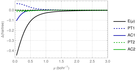
Figure 1: Errors of different approximations for the two-electron harmonium ($\omega=1/2$). The full black curve indicates the error of the model, $E(\mu)$. Blue curves correspond to first-order: dashed curve for perturbation theory, $\langle\Psi(\mu)|H|\Psi(\mu)\rangle$, full curve for first-order adiabatic connection, eq. (27). Green curves correspond to second-order: dashed curve for perturbation theory, eq. (15), full curve for second-order adiabatic connection, eq. (28).

Fig. 1 shows the general trends of the approximations. One can see, that by the choice of using the bare field, $v$, for all values of $\mu$, cf. eq. (9), the error of the model in the limit of small $\mu$ is catastrophic (0.5 hartree). First-order perturbation theory leads to the expectation value of the physical Hamiltonian, and thus gives an upper bound to the exact energy. In spite of using a bad wave function, the improvement is important: the error is decreased by an order of magnitude to $\approx 0.06$ hartree. Hartree-Fock, the best value that can be obtained for the non-interacting wave function, is in error by $\approx 0.04$ hartree. Second-order perturbation theory further improves the result.

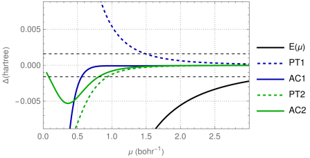
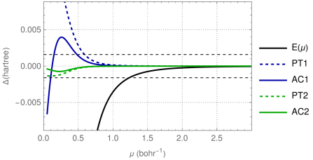
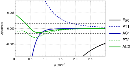
Figure 2: Errors of different approximations for the two-electron harmonium ($\omega=1/2$). The full black curve indicates the error of the model, $E(\mu)$. Blue curves correspond to first-order: dashed curve for perturbation theory, $\langle\Psi(\mu)|H|\Psi(\mu)\rangle$, full curve for first-order adiabatic connection, eq. (27). Green curves correspond to second-order: dashed curve for perturbation theory, eq. (15), full curve for second-order adiabatic connection, eq. (28). Top panel: ground state; middle panel: first excited state with $\ell=1$; bottom panel: first excited state with $\ell=0$.

The range of chemical accuracy cannot be distinguished on the scale of the plot shown in fig. 1. In order to discuss the suitability of the results, we have to zoom in (see fig. 2, top). We notice that for the ground state (a singlet state, $\ell=0$), the model does not reach chemical accuracy for the whole range of $\mu$ shown in the plot. The result of the first-order perturbation theory is improved by using the correction established for $\mu\rightarrow\infty$, eq. (27). Surprisingly, in spite of using an expansion in $1/\mu$, the error remains negligible even for some range of $\mu<1$ bohr^-1 (to $\approx 0.5$ bohr^-1). However, at smaller $\mu$ it worsens dramatically. Going over to the second-order perturbation theory improves over the first-order perturbation theory. Correcting asymptotically, eq. (28) improves the result over the whole range of values. However, chemical accuracy is not yet reached for all models.

Let us now apply the method to excited states. The model works much better for first triplet excited state ($\ell=1$), see fig. 2 (middle panel). This improves the results for all approximations.

Considering the first singlet excited state with $\ell=0$, fig. 2 (bottom), we notice that the quality of the model is worse than for the ground state. The corresponding curve does not even show up in the plot. However, the approximations show a behavior that roughly follows that of the ground state. We would like to stress that the corrections for the ground state and for the first excited state with $\ell=0$ use the same factors $\alpha_{\ell}^{(K)}$, eq. (29). The corrections are, of course, different, as the system-specific information enters through the model-specific quantities, $\partial^{K}E_{\ell}(\lambda,\mu)|_{\lambda=0}$.

4 Conclusion

The integral form of the remainder in Taylor’s expansion, eq. (13) provides a formula that generalizes the adiabatic connection. We use it to construct approximations to correct energies produced by model Hamiltonians with long range interaction, eqs. (27) and (28). They are inspired by approximations used in density functional theory. However, they do not use the Hohenberg-Kohn theorem, and are valid for the ground and excited states. Instead, they are constructed to be valid for the short-range interaction, as one approaches the physical system.

Results are shown only for harmonium. One can notice an improvement with increasing order of the adiabatic connection. No comparison is made with analogous density functional approximations. These can be found in ref. Sav-JCP-20, .

Of course, one would like to apply the method not only to harmonium. In other systems the sum in eq. (18) is extended over all values of $\ell$. An explicit treatment of the higher terms is difficult, may be too expensive computationally, and is maybe not needed – as it was alredy discussed, these terms are usually much smaller than the leading one. Thus, techniques such as described in refs. McWKut-IJQC-68, , and Ten-JCP-04, could be applied.

A strength of the method presented here is the stability of the result for large $\mu$. Once the stability is lost, it may indicate a worsening of the approximation.

A weakness of the method presented here is that it does not work sufficiently well (within chemical accuracy) for the non-interacting system ($\mu=0$). This makes the method more expensive. This feature is also present in range-separated density functional methods which possess a striking similarity with the one presented here. One may wonder if the experience gained by constructing density functional approximations cannot be exploited here, too. In particular, a properly constructed effective one-body potential in the model Hamiltonian can reduce the energy error of the physical (interacting) system (see, e.g., figs. 11 and 12 in ref. Sav-JCP-20, ). Alternatively, the method presented here could be used to improve density functional approximations.

Finally, we would like to point out that eq. (28) can be seen as a theoretical justification for spin-component-scaled methods GriGoeFin-12 .

5 Acknowledgement

We dedicate this paper to John P. Perdew who transformed the adiabatic connection to a useful tool not only in understanding DFT, but also for constructing approximations that changed the impact of computational chemistry and physics.

*

Appendix A A derivation of equation (19)

We generalize for an arbitrary $\ell$ the results obtained for $\ell=0$ in Section III of ref.3, and in Appendix of ref.18. We consider the behavior at the limit of large $\mu$ of the radial wave function $\varphi(r;\lambda,\mu)$ which is a solution of the radial Schrödinger equation (20)

$$\left[\mathsf{t}_{\ell}(r)+v_{\mathrm{int}}(r;\lambda,\mu)+\mathcal{R}(r)\right]\varphi_{\ell}(r;\lambda,\mu)=0,$$ (32)

where

$$\mathsf{t}_{\ell}(r)=-\partial_{r}^{2}-\frac{2}{r}\partial_{r}+\frac{\ell(\ell+1)}{r^{2}},$$ (33)

is the radial part of the kinetic energy operator corresponding to a given $\ell$,

$$v_{\mathrm{int}}(r;\lambda,\mu)=w(r;\mu)+\lambda\mathchoice{{\displaystyle\mkern 1.5mu\vbox{ \hrule height=0.8pt\vskip 0.57222pt\hbox{\set@color$\displaystyle\mkern-1.5muw\mkern-1.5mu$}}\mkern 1.5mu}}{{\textstyle\mkern 1.5mu\vbox{ \hrule height=0.8pt\vskip 0.57222pt\hbox{\set@color$\textstyle\mkern-1.5muw\mkern-1.5mu$}}\mkern 1.5mu}}{{\scriptstyle\mkern 1.5mu\vbox{ \hrule height=0.8pt\vskip 2.76805pt\hbox{\set@color$\scriptstyle\mkern-1.5muw\mkern-1.5mu$}}\mkern 1.5mu}}{{\scriptscriptstyle\mkern 1.5mu\vbox{ \hrule height=0.8pt\vskip 3.80138pt\hbox{\set@color$\scriptscriptstyle\mkern-1.5muw\mkern-1.5mu$}}\mkern 1.5mu}}(r;\mu)=\frac{(1-\lambda)\,\mathrm{erf}(\mu\,r)+\lambda}{r},$$ (34)

is the interaction potential, and $\mathcal{R}(r)$ is finite at $r=0$.

After changing variable $r$ to $x=\mu\,r$ and defining

$$u_{\ell}(x;\lambda,\mu)=\varphi_{\ell}(x/\mu;\lambda,\mu)$$ (35)

eq. (32) becomes

$$\mathsf{t}_{\ell}(x)\,u_{\ell}(x;\lambda,\mu)=\left[\frac{1}{\mu}\,v_{\mathrm{int}}(x;\lambda,1)+\mathcal{O}\left(\mu^{-2}\right)\right]\,u_{\ell}(x;\lambda,\mu).$$ (36)

To solve eq. (36) we use the first-order perturbation theory with perturbation parameter $1/\mu$. We set

$$u_{\ell}(x;\lambda,\mu)=u^{(0)}_{\ell}(x)+\frac{1}{\mu}\,u^{(1)}_{\ell}(x;\lambda)+\mathcal{O}(\mu^{-2}),$$ (37)

where $u^{(0)}_{\ell}(x)$ and $u^{(1)}_{\ell}(x;\lambda)$ are solutions of the zeroth and the first order perturbation equations:

$$\mathsf{t}_{\ell}(x)\,u^{(0)}_{\ell}(x)=0,$$ (38)

$$\mathsf{t}_{\ell}(x)\,u^{(1)}_{\ell}(x;\lambda)=F(x;\lambda),$$ (39)

and

$$F(x;\lambda)=v_{\mathrm{int}}(x;\lambda,1)\,u^{(0)}_{\ell}(x).$$ (40)

The general solution of the second-order homogeneous differential equation (38) is a linear combination of its two independent solutions: $f_{1}(x)=x^{\ell}$, and $f_{2}(x)=x^{-(l+1)}$:

$$u^{(0)}_{\ell}(x)=\mathcal{A}^{(1)}_{\ell}\,f_{1}(x)+\mathcal{A}_{\ell}^{(2)}\,f_{2}(x).$$ (41)

The inhomogeneous equation (39) is solved in quadratures:

$$u^{(1)}_{\ell}(x;\lambda) = f_{1}(x)\,\left[\mathcal{B}^{(1)}_{\ell}(\lambda)-\int\,\frac{f_{2}(x)}{\mathcal{W}(x)}\,F(x;\lambda)\,dx\right]$$

$$+ f_{2}(x)\,\left[\mathcal{B}^{(2)}_{\ell}(\lambda)+\int\,\frac{f_{1}(x)}{\mathcal{W}(x)}\,F(x;\lambda)\,dx\right],$$

where

$$\mathcal{W}(x)=f_{1}(x)\,\frac{df_{2}(x)}{dx}-f_{2}(x)\,\frac{df_{1}(x)}{dx}=-\frac{2\ell+1}{x^{2}}$$

is the Wronskian of solutions of the homogeneous equation.

According to eqs. (34) and (40),

$$F(x;\lambda)=(1-\lambda)\,F(x;0)+\lambda\,F(x;1).$$ (43)

Consequently, from eq. (A) we have

$$u^{(1)}_{\ell}(x;\lambda)=(1-\lambda)\,u^{(1)}_{\ell}(x;0)+\lambda\,u^{(1)}_{\ell}(x;1).$$ (44)

Notice that also

$$\mathcal{B}^{(i)}_{\ell}(\lambda)=(1-\lambda)\,\mathcal{B}^{(i)}_{\ell}(0)+\lambda\,\mathcal{B}^{(i)}_{\ell}(1),\;\;\;i=1,2,$$ (45)

where $\mathcal{B}^{(i)}_{\ell}(0)$ and $\mathcal{B}^{(i)}_{\ell}(1)$ depend on neither $\lambda$ nor $\mu$.

The integration constants $\mathcal{A}^{(i)}_{\ell}$ and $\mathcal{B}^{(i)}_{\ell}$, $i=1,2$, are determined from the requirement that the wave function fulfills the coalescence conditionsKurNakNak-AQC-16 ; SavKar-23 . In particular, neither $u^{(0)}_{\ell}(x)$ nor $u^{(1)}_{\ell}(x;\lambda)$ can be singular at $x=0$. The last requirement implies that $\mathcal{A}^{(2)}=0$.

The evaluation of $\lambda=1$ contribution is straightforward. We have

$$u^{(1)}_{\ell}(x;1)=\frac{1}{2\ell+1}\left[\mathcal{B}^{(1)}_{\ell}(1)x^{\ell}+\frac{\mathcal{B}^{(2)}_{\ell}(1)}{x^{\ell+1}}\right]+\frac{\mathcal{A}^{(1)}_{\ell}\,x^{\ell+1}}{2\ell+2}.$$ (46)

On the other hand, according to eq. (26) of ref.18,

$$u^{(1)}_{\ell}(x;1)\,\propto\,\frac{r^{\ell+1}}{2\ell+2}$$

(the Kato’s cusp conditionKat-CPAM-57 ). Therefore, in order to recover the correct behavior of the Coulomb radial function at small $x$, we have to set $\mathcal{B}^{(1)}_{\ell}(1)=\mathcal{B}^{(2)}_{\ell}(1)=0$. Finally, according to eqs. (37), (41), and (46),

$$u_{\ell}(x;1,\mu)=\mathcal{A}^{(1)}_{\ell}\,x^{\ell}\,\left[1+\frac{x}{\mu\,(2\ell+2)}\right]+\mathcal{O}(\mu^{-2}).$$ (47)

The second contribution, corresponding to $\lambda=0$, is more difficult to calculate. At the limit of large $\mu$, and for sufficiently large $r$, $\varphi(r;0,\mu)\rightarrow\varphi(r;1,\mu)$ GorSav-PRA-06 To meet this condition we have to set $\mathcal{B}^{(1)}_{\ell}(0)=0$. By fixing

$$\mathcal{B}^{(2)}_{\ell}(0)=-\mathcal{A}^{(1)}_{\ell}\,\frac{\Gamma(\ell+3/2)}{(2\ell+2)\sqrt{\pi}},$$ (48)

and using properties of the incomplete gamma function (see, for example, ref. 4, or https://functions.wolfram.com/GammaBetaErf/Erf/21/01/02/01/01/01/) we get an explicit, non-singular, expression

$$u^{(1)}_{\ell}(x;0)=\frac{\mathcal{A}^{(1)}_{\ell}\,x^{\ell}}{\sqrt{\pi}}\left[\frac{\sqrt{\pi}\,x\,\mathrm{erf}(x)}{2\ell+2}+\frac{\mathrm{e}^{-x^{2}}}{(2\ell+1)}+\frac{\Gamma(\ell+3/2)-\Gamma(\ell+3/2,x^{2})}{(2\ell+1)(2\ell+2)x^{2\ell+1}}\right].$$ (49)

By expanding the right-hand side of eq. (49) to a power series of $x$, we get

$$u^{(1)}_{\ell}(x;0)=\frac{\mathcal{A}^{(1)}_{\ell}\,x^{\ell}}{\sqrt{\pi}}\sum_{n=0}\,\frac{(-1)^{n+1}\,x^{2n}}{(2n-1)(2n+2\ell+1)\,n!}.$$ (50)

Alternatively, eq. (50) can be obtained by the expansion of $F(x,0)$ and subsequent evaluation of integrals in eq. (A). Notice, that the integration constants in both approaches are different.

For $\ell=0,1,2,\ldots$ eq. (49) can be simplified using the recurrence relation given in ref. 4:

$$\Gamma(1/2,x^{2})=\sqrt{(}\pi)\,(1-\mathrm{erf}(x)),\;\;\;\;\;\;\Gamma\left(a+1,x^{2}\right)=a\,\Gamma\left(a,x^{2}\right)+x^{2a}\,\mathrm{e}^{-x^{2}}.$$ (51)

$$u^{(1)}_{0}(x;0) = \frac{\mathcal{A}^{(1)}_{\ell}}{2}\left[\left(x+\frac{1}{2\,x}\right)\,\mathrm{erf}(x)+\frac{\mathrm{e}^{-x^{2}}}{\sqrt{\pi}}\right],$$ (52)

$$u^{(1)}_{1}(x;0) = \frac{\mathcal{A}^{(1)}_{\ell}\,x}{4}\left[\left(x+\frac{1}{4\,x^{3}}\right)\,\mathrm{erf}(x)+\frac{\mathrm{e}^{-x^{2}}}{\sqrt{\pi}}\left(1-\frac{1}{2\,x^{2}}\right)\right],$$ (53)

$$u^{(1)}_{2}(x;0) = \frac{\mathcal{A}^{(1)}_{\ell}\,x^{2}}{6}\left[\left(x+\frac{3}{8\,x^{5}}\right)\,\mathrm{erf}(x)+\frac{\mathrm{e}^{-x^{2}}}{\sqrt{\pi}}\left(1-\frac{1}{2\,x^{2}}-\frac{3}{4\,x^{4}}\right)\right].$$ (54)

Combining eqs. (37), (41), (44), (46), and (50) we get, at the limit of $r\rightarrow{0}$,

$$\varphi_{\ell}(r;\lambda,\mu)\,\propto\,r^{\ell}\,\left[1+\frac{1-\lambda}{\mu\sqrt{\pi}(2\ell+1)}+\frac{\lambda\,r}{2\ell+2}\right].$$ (55)

References

• (1) A. D. Becke. "Hartree-Fock exchange energy of an inhomogeneous electron gas". Int. J. Quantum Chem., 23:1915, 1983.
• (2) M. Ernzerhof and J. P. Perdew. "Generalized gradient approximation to the angle- and system-averaged exchange hole". J. Chem. Phys., 109:3313, 1998.
• (3) P. Gori-Giorgi and A. Savin. "Properties of short-range and long-range correlation energy density functionals from electron-electron coalescence". Phys. Rev. A, 73:032506, 2006.
• (4) I. S. Gradshteyn and I. M. Ryzhik. "The incomplete gamma function". In A. Jeffrey and D. Zwillinger, editors, Table of Integrals, Series and Products. Elsevier, Academic Press, Amsterdam, 2007.
• (5) S. Grimme, L. Goerigk, and R. F. Fink. "Spin-component-scaled electron correlation methods". Wiley Interdiscip. Rev.: Comput. Mol. Sci., 2:886, 2012.
• (6) O. Gunnarsson and B. I. Lundqvist. "Exchange and correlation in atoms, molecules, and solids by the spin-density-functional formalism". Phys. Rev. B, 13:4274, 1976.
• (7) P. Güttinger. "Das Verhalten von Atomen im magnetischen Drehfeld". Z. Phys., 73:169, 1932.
• (8) J. Harris and R. O. Jones. "The surface energy of a bounded electron gas". J. Phys. F, 4:1170, 1974.
• (9) P. Hohenberg and W. Kohn. "Inhomogeneous electron gas". Phys. Rev., 136:B864, 1964.
• (10) T. Kato. "On the eigenfunctions of many-particle systems in quantum mechanics". Comm. Pure Appl. Math., 10:151, 1957.
• (11) Y. I. Kurokawa, H. Nakashima, and H. Nakatsuji. "General coalescence conditions for the exact wave functions: Higher-order relations for Coulombic and non-Coulombic systems". Adv. Quantum Chem., 73:59, 2016.
• (12) W. Kutzelnigg and J. D. Morgan III. "Rates of convergence of the partial-wave expansions of atomic correlation energies". J. Chem. Phys., 96:4484, 1992.
• (13) D. C. Langreth and J. P. Perdew. "The exchange-correlation energy of a metallic surface". Solid State Commun., 17:1425, 1975.
• (14) R. McWeeny and W. Kutzelnigg. "Symmetry properties of natural orbitals and geminals. I. Construction of spin- and symmetry-adapted functions". Int. J. Quantum Chem., 2:187, 1968.
• (15) R. T. Pack and W. Byers Brown. "Cusp conditions for molecular wave functions". J. Chem. Phys., 45:556, 1966.
• (16) J. A. Pople. "Nobel lecture: Quantum chemical models". Rev. Mod. Phys., 71:1267, 1999.
• (17) A. Savin. "Models and corrections: Range separation for electronic interaction — Lessons from density functional theory". J. Chem. Phys., 153:160901, 2020.
• (18) A. Savin and J. Karwowski. "Correcting models with long-range electron interaction using generalized cusp conditions". J. Phys. Chem. A, 127:1377, 2023.
• (19) I. Silanes, J. M. Ugalde, and R. J. Boyd. "Cusp conditions for non-Coulombic interactions". J. Mol. Struct. (Theochem), 527:27, 2000.
• (20) S. Ten-no. "Explicitly correlated second order perturbation theory: Introduction of a rational generator and numerical quadratures". J. Chem. Phys., 121:117, 2004.
• (21) T. Ziegler, A. Rauk, and E. J. Baerends. "On the calculation of multiplet energies by the Hartree-Fock-Slater method". Theor. Chim. Acta, 43:261, 1977.