Highly Efficient Creation and Detection of Ultracold Deeply-Bound Molecules via Chainwise Stimulated Raman Shortcut-to-Adiabatic Passage

Abstract

Chainwise stimulated Raman adiabatic passage (C-STIRAP) in M-type molecular system is a good alternative in creating ultracold deeply-bound molecules when the typical STIRAP in $\Lambda$-type system does not work due to weak Frank-Condon factors between states. However, its creation efficiency under the smooth evolution is generally low. During the process, the population in the intermediate states may decay out quickly and the strong laser pulses may induce multi-photon processes. In this paper, we find that shortcut-to-adiabatic (STA) passage fits very well in improving the performance of the C-STIRAP. Currently, related discussions on the so-called chainwise stimulated Raman shortcut-to-adiabatic passage (C-STIRSAP) are rare. Here, we investigate this topic under the adiabatic elimination. Given a relation among the four incident pulses, it is quite interesting that the M-type system can be generalized into an effective $\Lambda$-type structure with the simplest resonant coupling. Consequently, all possible methods of STA for three-state system can be borrowed. We take the counter-diabatic driving and “chosen path” method as instances to demonstrate our treatment on the molecular system. Although the “chosen path” method does not work well in real three-state system if there is strong decay in the excited state, our C-STIRSAP protocol under both the two methods can create ultracold deeply-bound molecules with high efficiency in the M-type system. The evolution time is shortened without strong laser pulses and the robustness of STA is well preserved. Finally, the detection of ultracold deeply-bound molecules is discussed.

I Introduction

The study of ultracold molecules is a rapidly developing area with fruitful research outcomes. There is great interest in their rich internal and motional quantum degrees of freedom, enabling the investigation of few-body collisional physics Blume (2012), ultracold chemistry Hutson (2010), precision measurements Ulmanis et al. (2012), quantum computations DeMille (2002) and quantum simulations Carr et al. (2009), to name a few. However, long-lived ensembles and full quantum state control are prerequisites to harness the potential of ultracold molecules. Therefore, cooling interacting molecular gases deeply into the quantum degenerate regime is required, which remains an elusive challenge Mitra et al. (2022).

Currently, a versatile approach for this purpose involves the atom-by-atom assembly of ultracold molecules from pre-cooled atoms. Initially, weakly-bound Feshbach molecules close to the atomic threshold are created via magnetically induced Feshbach association Jones et al. (2006). Subsequently, the Feshbach molecules are quickly transferred into ultracold deeply-bound molecules, in which the population lies in the lowest energy level of the electronic ground state. Note only in this state can collisional stability be ensured. As for other states, the molecules will undergo fast inelastic collisions that lead to trap loss. Over the past few years, the well-known stimulated Raman adiabatic passage (STIRAP) Král et al. (2007) has become the most widely used technique. Under the Stokes and pump pulse with counter-intuitive time sequence, the population in the Feshbach state can be completely transferred into the deeply-bound ground state without populating the intermediate excited state. The STIRAP has been successfully demonstrated for species such as homonuclear Rb₂, Cs₂, Sr₂ and Li₂ Winkler et al. (2007); Thalhammer et al. (2006); Lang et al. (2008); Danzl et al. (2008); Stellmer et al. (2012); Polovy et al. (2020), as well as heteronuclear KRb, RbCs, NaK, RbSr, NaRb, NaLi, RbHg, LiK, and NaCs Aikawa et al. (2010); Ospelkaus et al. (2008); Ni et al. (2008); Molony et al. (2016); Seeßelberg et al. (2018); Liu et al. (2019); Park et al. (2015); Guo et al. (2016); Rvachov et al. (2017); Yang et al. (2020); Cairncross et al. (2021); Stevenson et al. (2023); Lam et al. (2022); Warner et al. (2023); Voges et al. (2020); Seeßelberg et al. (2018).

Nevertheless, the STIRAP is such an adiabatic passage that it has to satisfy the adiabatic condition for perfect transfer. Therefore, the process usually evolves smoothly, rendering it intrinsically time consuming Král et al. (2007). In reality, the requirement usually results in imperfect transfer due to the presence of spontaneous emission and collision Dou et al. (2012, 2013); Zhang and Dou (2021). Moreover, the violation of the evolution along the dark state also leads to imperfect transfer if the adiabatic condition is not fulfilled Takekoshi et al. (2014).

In order to overcome the problem associated with the adiabatic passage, a technique which is called shortcut-to-adiabaticity (STA) was proposed Guéry-Odelin et al. (2019). The STA can speed up the adiabatic process while maintaining consistent results. Besides, the robustness of the adiabatic passage is also preserved even if the employed parameters do not meet the adiabatic condition. Nowadays, the STA has been extensively studied and various methods have been raised for different purposes. For instance, the counter-diabatic driving, or equivalently the transitionless quantum algorithm, is a commonly used method Demirplak and Rice (2003, 2005, 2008); Berry (2009); Chen et al. (2010); Masuda and Rice (2015). It usually requires an additional counter-diabatic field to directly couple the initial and target state to remove the non-adiabatic effect. Except for this, there are also methods such as invariant-based inverse engineering Lewis and Riesenfeld (1969); Chen et al. (2011); Chen and Muga (2012); Ho and Tseng (2015); Lu et al. (2017), multiple Schrödinger dynamics Ibáñez et al. (2012); Song et al. (2016), superadiabatic dressed states Baksic et al. (2016); Zhou et al. (2017) and three-mode parallel paths Wu et al. (2019, 2017); Tang et al. (2022). Based on these methods, the application of STA into the STIRAP has been suggested Li and Chen (2016) and successfully demonstrated in experiment Du et al. (2016).

When employing the STIRAP to create ultracold deeply-bound molecules, it is also crucial to note that the excited state, which serves as a bridge for the transfer, should be suitably identified. The excited state should have favorable transition dipole moments and good Frank-Condon overlaps with the vibrational wavefunctions of the Feshbach and ground molecular state Stwalley (2004). Customarily, this requirement is uneasy to meet due to the large difference in the average extension of the Feshbach and ground state. If such an excited state can not be provided for an efficient transfer, people can turn to using more intermediate states to form a M-type structure to overcome this technical challenge. Under the chainwise coupling, the Feshbach state can also be transferred into the ground state by using multiple Raman adiabatic passages Danzl et al. (2010); Kuznetsova et al. (2008); Mackie and Phou (2010). This method, stemming from the studies of STIRAP in atomic systems, is known as chainwise STIRAP (C-STIRAP) Malinovsky and Tannor (1997); Shore et al. (1991); Pillet et al. (1993); Oreg et al. (1985). However, the creation efficiency of the C-STIRAP is generally low Danzl et al. (2010). The main reason is that the intermediate states are populated during the multiple-step process. The spontaneous emission and collision then reduce the transfer efficiency under the long evolution time. Although increasing the coupling between the intermediate states can suppress the population in these states, it may be problematic for molecules because multi-photon processes are expected to occur to break the process Garraway and Suominen (1998).

According to the unique properties of the STA mentioned above, we find that the STA is quite suitable to solve the problems that the C-STIRAP encountered in its applications. Undoubtedly, it would be of interest if the STA can speed up the C-STIRAP to reduce the population loss from the intermediate states by avoiding using strong coupling pulses. Currently, related studies are quite few Vitanov (2020) and this topic deserves more investigations.

In this paper, we combine the STA with C-STIRAP in the M-type molecular system, which we call the chainwise stimulated Raman shortcut-to-adiabatic passage (C-STIRSAP), to study the creation of ultracold deeply-bound molecules with high efficiency. We first reduce the M-type system into an effective $\Lambda$-type system under the adiabatic elimination (AE). By doing so, the major population decay in the excited states out of the system can be suppressed. If we further set a requirement towards the relation among the four incident pulses, the effective $\Lambda$-type system will possess the simplest resonant couplings. This generalized model permits us to borrow all possible methods of STA from three-state system into the M-type system. We take the counter-diabatic driving and “chosen path” method as examples to demonstrate the feasibility of the C-STIRSAP. Note in real three-state system, the “chosen path” method can not realize perfect transfer if the excited state has a strong decay. However, numerical calculations show here that our protocol under the two methods can both create ultracold deeply-bound molecules with nearly perfect efficiency in the M-type system. Moreover, the process is speeded up without strong laser pulses and the robustness of STA is still maintained. Since the STA usually requires accurate control of the incident pulses, the requirement of the relation among the pulses in our protocol actually does not add extra experimental complexity. Finally, we discuss the detection of ultracold deeply-bound molecules.

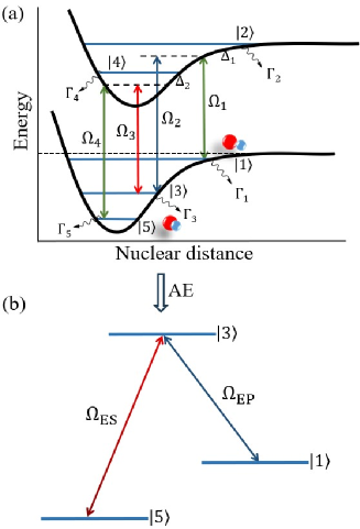
Figure 1: (a) Schematic diagram of the M-type molecular system with chainwise coupling. (b) Effective $\Lambda$-type system with resonant couplings $\Omega_{\rm{EP}}$ and $\Omega_{\rm{ES}}$ after the AE.

II generalization of the model

We start by considering the M-type molecular structure with chainwise coupling as illustrated in Fig. 1(a). Here, $|j\rangle(j=1,3,5)$ is the vibrational state of the ground electronic molecular state. To be more accurate, $|1\rangle$, $|3\rangle$ and $|5\rangle$ are the Feshbach state, an intermediate state and the deeply-bound ground state, respectively. $|j\rangle(j=2,4)$ is the vibrational state of an excited electronic molecular state. As a bridge of the transfer, the two excited states are assumed to have good Franck-Condon factors with the three ground states. The coupling between states is presented by the time-dependent Rabi frequency $\Omega_{j}(j=1,2,3,4)$ in this figure. Without loss of generality, all the states have decays $\Gamma_{j}(j=1,2,3,4,5)$ out of the molecular system due to spontaneous emissions and inelastic collisions. Nevertheless, we temporarily ignore them in the theoretical analysis in order to clarify the underlying physics.

The evolution of the molecular system is governed by the time-dependent Schrödinger equation

$$i\hbar\displaystyle\frac{\partial}{\partial t}|\Phi(t)\rangle=H(t)|\Phi(t)\rangle.$$ (1)

In this equation, $|\Phi(t)\rangle$ is the molecular wave function with the expanding form $|\Phi(t)\rangle=\sum_{j}a_{j}(t)|j\rangle(j=1,2,3,4,5)$, where $a_{j}(t)(j=1,2,3,4,5)$ represents the probability amplitude of the corresponding state. The two $\Lambda$-type substructures $|1\rangle\leftrightarrow|2\rangle\leftrightarrow|3\rangle$ and $|3\rangle\leftrightarrow|4\rangle\leftrightarrow|5\rangle$ in the molecular system are supposed to satisfy the two-photon resonance condition, as required by the C-STIRAP technique. Under the rotating wave approximation, Eq. (1) can be written as following

$$i\frac{d}{dt}\left(\begin{array}[]{ccccc}a_{1}\\ a_{2}\\ a_{3}\\ a_{4}\\ a_{5}\\ \end{array}\right)=\left(\begin{array}[]{ccccc}0&\Omega_{1}&0&0&0\\ \Omega_{1}&\Delta_{1}&\Omega_{2}&0&0\\ 0&\Omega_{2}&0&\Omega_{3}&0\\ 0&0&\Omega_{3}&\Delta_{2}&\Omega_{4}\\ 0&0&0&\Omega_{4}&0\\ \end{array}\right)\left(\begin{array}[]{ccccc}a_{1}\\ a_{2}\\ a_{3}\\ a_{4}\\ a_{5}\\ \end{array}\right).$$ (17)

in which $\Delta_{1}$ and $\Delta_{2}$ are the single-photon detunings of the corresponding transitions. We can clearly see from this equation that the Rabi frequency always connects one of the ground states with one of the excited states to form the chainwise coupling.

In order to apply the STA into the C-STIRAP, we are going to treat the above Hamiltonian in another way around, which is different from that in Ref. Vitanov (2020). We first consider the use of AE condition Mackie and Phou (2010) under the assumption that the two detunings $\Delta_{1}$ and $\Delta_{2}$ are large, which is

$$|\Delta_{1}|\gg\sqrt{\Omega_{1}^{2}+\Omega_{2}^{2}}$$ (18)

and

$$|\Delta_{2}|\gg\sqrt{\Omega_{3}^{2}+\Omega_{4}^{2}},$$ (19)

respectively. For simplicity, we assume that $\Delta_{1}=\Delta_{2}=\Delta$. After the AE, the population in the excited states is minimized and the decay out of the system can be greatly suppressed. By setting $\frac{d}{dt}a_{2}=\frac{d}{dt}a_{4}=0$, the molecular system can be reduced to an effective $\Lambda$-type structure which includes only ground states $|j\rangle(j=1,3,5)$ as shown in Fig. 1(b). The Schrödinger equation is simplified as

$$i\frac{d}{dt}\left(\begin{array}[]{ccc}a_{1}\\ a_{3}\\ a_{5}\\ \end{array}\right)=\left(\begin{array}[]{ccc}\beta_{1}&\Omega_{\rm{EP}}&0\\ \Omega_{\rm{EP}}&\beta_{3}&\Omega_{\rm{ES}}\\ 0&\Omega_{\rm{ES}}&\beta_{5}\\ \end{array}\right)\left(\begin{array}[]{ccc}a_{1}\\ a_{3}\\ a_{5}\\ \end{array}\right).$$ (29)

In this equation, the $3\times 3$ matrix is the effective Halmiltonian with the three diagonal elements being defined as $\beta_{1}=-\frac{\Omega_{1}^{2}}{\Delta}$, $\beta_{3}=-\frac{\Omega_{2}^{2}+\Omega_{3}^{2}}{\Delta}$ and $\beta_{5}=-\frac{\Omega_{4}^{2}}{\Delta}$, respectively. $\Omega_{\rm{EP}}$ and $\Omega_{\rm{ES}}$ can be considered as Rabi frequencies induced by an effective pump and Stokes pulse and they are expressed as $\Omega_{\rm{EP}}=-\frac{\Omega_{1}\Omega_{2}}{\Delta}$ and $\Omega_{\rm{ES}}=-\frac{\Omega_{3}\Omega_{4}}{\Delta}$. We can find that the direct couplings between the ground and excited states now disappear and there are only effective couplings between the ground states $|1\rangle\leftrightarrow|3\rangle$ and $|3\rangle\leftrightarrow|5\rangle$.

We can continue to simplify the analysis if the three diagonal elements are equal to each other, which is $\beta_{1}=\beta_{3}=\beta_{5}=\beta$. This requires that the four Rabi frequencies $\Omega_{j}(j=1,2,3,4)$ should satisfy the following relation

$$\Omega_{1}=\Omega_{4}=\sqrt{\Omega_{2}^{2}+\Omega_{3}^{2}}.$$ (30)

By further setting $a_{j}=c_{j}e^{-i\beta t}(j=1,3,5)$, Eq. (29) can be rewritten as

$$\begin{split}i\frac{d}{dt}\left(\begin{array}[]{ccc}c_{1}\\ c_{3}\\ c_{5}\\ \end{array}\right)=\left(\begin{array}[]{ccc}0&\Omega_{\rm{EP}}&0\\ \Omega_{\rm{EP}}&0&\Omega_{\rm{ES}}\\ 0&\Omega_{\rm{ES}}&0\\ \end{array}\right)\left(\begin{array}[]{ccc}c_{1}\\ c_{3}\\ c_{5}\\ \end{array}\right).\end{split}$$ (31)

The two parameters $\Omega_{\rm{EP}}$ and $\Omega_{\rm{ES}}$ are changed to be

$$\Omega_{\rm{EP}}=-\frac{\Omega_{2}\sqrt{\Omega_{2}^{2}+\Omega_{3}^{2}}}{\Delta}$$ (32)

and

$$\Omega_{\rm{ES}}=-\frac{\Omega_{3}\sqrt{\Omega_{2}^{2}+\Omega_{3}^{2}}}{\Delta}$$ (33)

respectively. Now the effective pump and Stokes pulse are resonant with the transitions $|1\rangle\leftrightarrow|3\rangle$ and $|3\rangle\leftrightarrow|5\rangle$.

Although we can reduce the M-type molecular system into the $\Lambda$-type system with the simplest resonant coupling as shown in Fig. 1(b), still we can not directly employ the standard STIRAP. Under the STIRAP, the $\Lambda$-type system is expected to evolve adiabatically along the dark state of the effective Hamiltonian in Eq. (31), which is

$$|\Phi_{0}\rangle=\cos\theta|1\rangle-\sin\theta|5\rangle$$ (34)

with the mixing angle being defined as $\tan\theta=\Omega_{\rm{EP}}/\Omega_{\rm{ES}}$. Nevertheless, we need to satisfy the adiabatic condition $\sqrt{\Omega_{\rm{EP}}^{2}+\Omega_{\rm{ES}}^{2}}\gg\dot{\theta}$ Král et al. (2007). The condition requires using strong laser pulses and it conflicts with the AE condition; see Eqs. (18) and (19). Therefore, the standard STIRAP is inappropriate for efficient creation of ultracold deeply-bound molecules here. It is of importance if the STA can be applied here to avoid the use of strong pulses.

III the C-STIRSAP

In this section, we are going to carry out the STA combined with the C-STIRAP in the M-type molecular system. We call the technique the chainwise stimulated Raman shortcut-to-adiabatic passage (C-STIRSAP). Based on the generalized three-state model in the above section, theoretically all kinds of methods in the frame of STA can be borrowed here. In the following, we will take the counter-diabatic driving, which is a widely used method, and the “chosen path” method as examples to illustrate the feasibility of the C-STIRSAP.

III.1 counter-diabatic driving

The basic idea of counter-diabatic driving in a three-state $\Lambda$-type system requires an auxiliary field to directly couple the two lower states as shown in Fig. 1(b) to eliminate the non-adiabatic couplings and make the adiabatic evolution possible. Following the steps introduced in Ref. Chen et al. (2010), we can obtain the expression of the auxiliary field

$$\Omega_{\rm{cd}}=\frac{\dot{\Omega}_{2}{\Omega}_{3}-\dot{\Omega}_{3}{\Omega}_{2}}{{\Omega}^{2}_{2}+{\Omega}^{2}_{3}},$$ (35)

in which the overdot means the time derivative of the parameter. Note that the auxiliary field now couples the Feshbach state $|1\rangle$ and the deeply-bound ground state $|5\rangle$. Assisted by the counter-diabatic field, the simplified $\Lambda$-type model governed by Eq. (31) now becomes

$$\begin{split}i\frac{d}{dt}\left(\begin{array}[]{ccc}c_{1}\\ c_{3}\\ c_{5}\\ \end{array}\right)=\left(\begin{array}[]{ccc}0&\Omega_{\rm{EP}}&i\Omega_{\rm{cd}}\\ \Omega_{\rm{EP}}&0&\Omega_{\rm{ES}}\\ -i\Omega_{\rm{cd}}&\Omega_{\rm{ES}}&0\\ \end{array}\right)\left(\begin{array}[]{ccc}c_{1}\\ c_{3}\\ c_{5}\\ \end{array}\right).\end{split}$$ (36)

Turning back to the real M-type molecular system as shown in Fig. 1(a), the description of Eq. (17) with the auxiliary field is now modified to be

$$i\frac{d}{dt}\left(\begin{array}[]{ccccc}a_{1}\\ a_{2}\\ a_{3}\\ a_{4}\\ a_{5}\\ \end{array}\right)=\left(\begin{array}[]{ccccc}0&\Omega_{1}&0&0&i\Omega_{\rm{cd}}\\ \Omega_{1}&\Delta&\Omega_{2}&0&0\\ 0&\Omega_{2}&0&\Omega_{3}&0\\ 0&0&\Omega_{3}&\Delta&\Omega_{4}\\ -i\Omega_{\rm{cd}}&0&0&\Omega_{4}&0\\ \end{array}\right)\left(\begin{array}[]{ccccc}a_{1}\\ a_{2}\\ a_{3}\\ a_{4}\\ a_{5}\\ \end{array}\right).$$ (52)

Note that $\Omega_{\rm{cd}}$ still couples the states $|1\rangle$ and $|5\rangle$. The above Schrödinger equation after the modification implies that we obtain a five-state counter-diabatic driving from that of the three-state system. The scheme is then supposed to achieve our goal that it can speed up the process and preserve the adiabaticity without fulfilling the adiabatic condition. In order to verify the C-STIRSAP using the counter-diabatic driving does work in the M-type molecular system, we are going to study the evolution of the M-type system by numerical calculations. Since the molecules suffer from unavoidable spontaneous emissions and collisions, the decays from states displayed in Fig. 1(a) should be taken into account. Therefore, we are going to employ the Liouville-von Neumann equation

$$\displaystyle\frac{d\rho}{dt}=-i[\tilde{H},\rho]-\Gamma\rho,$$ (53)

for the calculations. In this equation, the modified Hamiltonian $\tilde{H}$ is the $5\times 5$ matrix in Eq. (52). $\rho$ is the density matrix operator and $\Gamma\rho$ is the operator describing the decaying processes. It is also a $5\times 5$ matrix with its element defined as $(\Gamma\rho)_{mn}=\frac{\Gamma_{m}+\Gamma_{n}}{2}\rho_{mn}(m,n=1,2,3,4,5)$.

We take the parameters of molecule ⁸⁷Rb₂ in the calculations Kuznetsova et al. (2008). The population of the system is assumed to be initially in the Feshbach state. As for the decay rates, the two excited states $|2\rangle$ and $|4\rangle$ have the shortest lifetime and their decay rates are chosen as $\Gamma_{2}=\Gamma_{4}=30{\rm{MHz}}$. The decay rates of the Feshbach state $|1\rangle$ and the intermediate state $|3\rangle$ are set to be $\Gamma_{1}=0.01{\rm{MHz}}$ and $\Gamma_{3}=0.06{\rm{MHz}}$, respectively. The deeply-bound ground state $|5\rangle$ has quite a long lifetime compared with the evolution time of the system. Therefore, we can safely ignore the decay from this state, which is $\Gamma_{5}=0$.

The two pulses with Rabi frequencies $\Omega_{2}$ and $\Omega_{3}$ are partially overlapped and their envelopes are Gaussian shaped, which are

$$\Omega_{\rm{2}}=\Omega_{0}\exp[-\frac{(t-t_{\rm{f}}/2-\tau)^{2}}{\sigma^{2}}]$$ (54)

and

$$\Omega_{\rm{3}}=\Omega_{0}\exp[-\frac{(t-t_{\rm{f}}/2+\tau)^{2}}{\sigma^{2}}],$$ (55)

respectively. Here, $\Omega_{0}$ is the amplitude of the Rabi frequency. $\sigma$ is the pulse duration. $2\tau$ is the time delay between the two pulses and $t_{\rm{f}}$ is the evolution time (or operation time) of the system. These parameters are chosen as $\Omega_{0}=30\pi{\rm{MHz}}$, $t_{\rm{f}}=1000\rm{ns}$, $\sigma=t_{\rm{f}}/6$ and $\tau=t_{\rm{f}}/10$. For the other two Rabi frequencies $\Omega_{\rm{1}}$ and $\Omega_{\rm{4}}$ and the auxiliary field $\Omega_{\rm{cd}}$, they are chosen accordingly with respect to Eqs. (30) and (35). Note that the operation time is short and the adiabaticity is broken down in this case. The detuning in the calculations is set to be $\Delta=2\pi{\rm{GHz}}$, which is much larger than those Rabi frequencies to meet the requirement of AE.

We first present the evolution of the M-type molecular system under the C-STIRSAP with counter-diabatic driving. The time sequence of the four Rabi frequencies and the auxiliary field is shown in Fig. 2(a). The corresponding population transfer in the system is displayed in Fig. 2(b). As a comparison, we also present the population evolution of the system under the C-STIRAP, which can be seen in Fig. 2(c). The calculation of C-STIRAP is carried out by simply excluding the auxiliary field in the modified Hamiltonian in Eq. (52) while all the other parameters are kept unchanged.

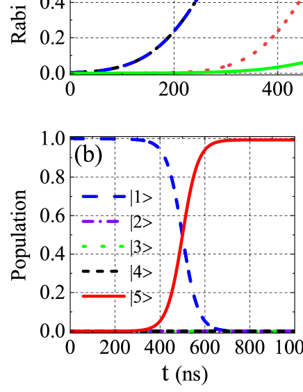
Figure 2: (a) Time sequence of the four Rabi frequencies $\Omega_{j}(j=1,2,3,4)$ together with the auxiliary field $\Omega_{\rm{cd}}$. (b) Population evolution under the C-STIRSAP by using the counter-diabatic driving while (c) is that under the C-STIRAP without considering the auxiliary field.

We can observe from Fig. 2(b) that we obtain nearly complete population transfer from the Feshbach state $|1\rangle$ to the ground state $|5\rangle$ without populating the intermediate state $|3\rangle$, indicating the creation of ultracold deeply-bound molecules with high efficiency. The population of the excited states, $|2\rangle$ and $|4\rangle$, is negligible in presence of the AE. On the contrary, the population transfer from the Feshbach state $|1\rangle$ to the ground state $|5\rangle$ hardly occurs in Fig. 2(c), although the intermediate state $|3\rangle$ is partly populated. The population in the excited states $|2\rangle$ and $|4\rangle$ is still negligible due to the AE. Clearly, the C-SRTRSAP with counter-diabatic driving can speed up the complete population transfer without using strong pulses.

Further calculations can show more properties of the C-STIRSAP with counter-diabatic driving. In Fig. 3(a), we study the transfer efficiency from the Feshbach state $|1\rangle$ to the ground state $|5\rangle$ as a function of the amplitude of Rabi frequency $\Omega_{0}$ under the C-STIRSAP and C-STIRAP, respectively. All the other parameters are kept the same as those in Fig. 2. We can roughly see from Fig. 3(a) that the transfer efficiency under the C-STIRSAP is always higher than that under the C-STIRAP. To be more precisely, nearly perfect transfer efficiency can always be obtained under the C-STIRSAP. The transfer efficiency slightly decreases with the increase of Rabi frequency $\Omega_{0}$. The reason is the AE condition is gradually destroyed while the detuning $\Delta$ is fixed unchanged, resulting in the population in other states. As for the transfer efficiency under the C-STIRAP, it behaves differently. Initially, it increases rapidly with the increase of Rabi frequency $\Omega_{0}$. The efficiency reaches its maximum which is about $94\%$ when the amplitude of the Rabi frequency is around $\Omega_{0}=125\pi{\rm{MHz}}$. This is because the adiabaticity of the C-STIRAP is approximately satisfied with the increase of the Rabi frequency and it starts to dominate the process. If we continue increasing the Rabi frequency, the efficiency starts to decrease, which is also due to the breakdown of the AE condition.

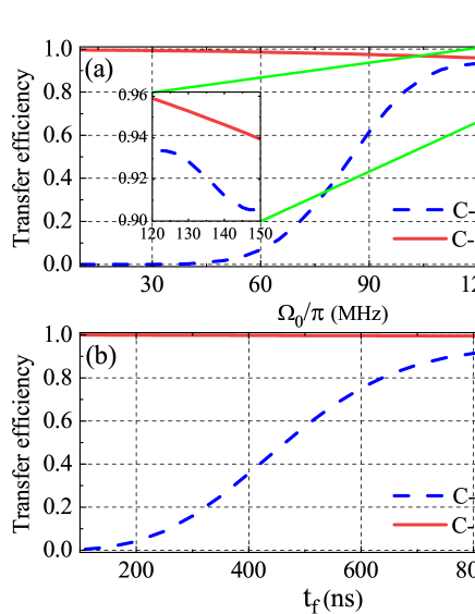
Figure 3: Transfer efficiency as functions of (a) the amplitude of Rabi frequency $\Omega_{0}$ and (b) the operation time $t_{\rm{f}}$ under the C-STIRSAP and C-STIRAP, respectively. Note that in (b) $\Omega_{0}$ is chosen as $30\pi{\rm{MHz}}$ for the C-STIRSAP while it is $125\pi{\rm{MHz}}$ for the C-STIRAP. All the other parameters are the same as those in Fig. 2.

In Fig. 3(b), we investigate the transfer efficiency as a function of the operation time $t_{\rm{f}}$ under the C-STIRSAP and C-STIRAP, respectively. Note the amplitude of Rabi frequency is chosen as $\Omega_{0}=30\pi{\rm{MHz}}$ for the C-STIRSAP, while we choose the optimal value of $\Omega_{0}=125\pi{\rm{MHz}}$ for the C-STIRAP, which corresponds to the maximum transfer efficiency in Fig. 3(a). The other parameters are kept unchanged as those in Fig. 2. We can see from Fig. 3(b) that perfect transfer efficiency can always be obtained regardless the choice of the operation time $t_{\rm{f}}$ under the C-STIRSAP. In contrast, the transfer efficiency increases slowly with the increase of the operation time $t_{\rm{f}}$ under the C-STIRAP, although the Rabi frequency $\Omega_{0}$ has been optimized. Clearly, the C-STIRAP is time-consuming in order to obtain high transfer efficiency.

The above calculations demonstrate that the C-STIRSAP with counter-diabatic driving works very well in efficiently creating ultracold deeply-bound molecules. Besides, the unique properties of STA are still preserved. The operation time is shortened while the process is robust against the fluctuations of parameters even if the adiabatic condition is not fulfilled. Nevertheless, we note that sometimes the direct coupling between states $|1\rangle$ and $|5\rangle$ by the auxiliary field is infeasible. There may be possibilities that the transition is difficult to achieve due to different spin characters or weak Franck-Condon factor between the states. Therefore, alternative methods other than the direct application of counter-diabatic pulse are necessary. In the following, we are going to take the “chosen path” method to give another solution to combine the STA with the C-STIRAP.

III.2 “chosen path” method

Unlike the counter-diabatic driving, the three-state “chosen path” method accelerates the adiabatic process by adding an extra pair of fields into the Rabi frequencies $\Omega_{\rm{EP}}$ and $\Omega_{\rm{ES}}$ Wu et al. (2019). This idea can also be found in other methods such as invariant-based inverse engineering Lewis and Riesenfeld (1969); Chen et al. (2011); Chen and Muga (2012); Ho and Tseng (2015); Lu et al. (2017), multiple Schrödinger dynamics Ibáñez et al. (2012); Song et al. (2016) and superadiabatic dressed states Baksic et al. (2016); Zhou et al. (2017). Although these methods have different mathematical treatments, they are strongly related since they possess similar underlying physics (see recent reviews Guéry-Odelin et al. (2019), Torrontegui et al. (2013) and Taras et al. (2021)). The two Rabi frequencies are then modified and the Schrödinger equation describing the reduced $\Lambda$-type model now has the form

$$\begin{split}i\frac{d}{dt}\left(\begin{array}[]{ccc}c_{1}\\ c_{3}\\ c_{5}\\ \end{array}\right)=\left(\begin{array}[]{ccc}0&\tilde{\Omega}_{\rm{EP}}&0\\ \tilde{\Omega}_{\rm{EP}}&0&\tilde{\Omega}_{\rm{ES}}\\ 0&\tilde{\Omega}_{\rm{ES}}&0\end{array}\right)\left(\begin{array}[]{ccc}c_{1}\\ c_{3}\\ c_{5}\\ \end{array}\right).\end{split}$$ (56)

The aim of “chosen path” method is that the simplified three-state system in Fig. 1(b) can evolve along one of its dressed states, which is

$$|\Phi^{\prime}_{0}\rangle= \cos\mu(t)\cos\theta(t)|1\rangle+i\sin\mu(t)|3\rangle$$ (57)

$$+\cos\mu(t)\sin\theta(t)|5\rangle.$$

Meanwhile, this dressed state $|\Phi^{\prime}_{0}\rangle$ is designed to be decoupled with the other two dressed statesWu et al. (2017). In order to transfer the population from the Feshbach state $|1\rangle$ to the deeply-bound ground state $|5\rangle$, the two time-dependent parameters $\mu(t)$ and $\theta(t)$ should satisfy the boundary condition, which is $\mu(0)=\mu(t_{\rm{f}})=0$ and $\theta(0)=0$ and $\theta(t_{\rm{f}})=\pi/2$. Following the steps in Ref. Wu et al. (2017), the two parameters can be defined as

$$\mu(t)=\frac{\gamma}{2}\left[1-\cos(\frac{2\pi t}{t_{\rm{f}}})\right]$$ (58)

and

$$\theta(t)=\frac{\pi t}{2t_{\rm{f}}}-\frac{1}{3}\sin(\frac{2\pi t}{t_{\rm{f}}})+\frac{1}{24}\sin(\frac{4\pi t}{t_{\rm{f}}}),$$ (59)

respectively. Then the corresponding two modified Rabi frequencies $\tilde{\Omega}_{\rm{EP}}$ and $\tilde{\Omega}_{\rm{ES}}$ with the following expressions

$$\tilde{\Omega}_{\rm{EP}}=-\dot{\theta}(t)\sin\theta(t)\cot\mu(t)-\dot{\mu}(t)\cos\theta(t)$$ (60)

and

$$\tilde{\Omega}_{\rm{ES}}=\dot{\theta}(t)\cos\theta(t)\cot\mu(t)-\dot{\mu}(t)\sin\theta(t)$$ (61)

can guarantee the evolution along the dressed state $|\Phi^{\prime}_{0}\rangle$. In Eq. (58), the parameter $\gamma$ should not be equal to zero. Otherwise, $\tilde{\Omega}_{\rm{EP}}$ and $\tilde{\Omega}_{\rm{ES}}$ will be infinitely large.

Now we go back to the M-type molecular system and try to design the modified Rabi frequencies $\tilde{\Omega}_{j}(j=1,2,3,4)$ by comparing the Hamiltonians in Eqs. (56) and (31). Similar to Eqs. (32) and (33), we can impose that

$$\tilde{\Omega}_{\rm{EP}}=-\frac{\tilde{\Omega}_{2}\sqrt{\tilde{\Omega}_{2}^{2}+\tilde{\Omega}_{3}^{2}}}{\tilde{\Delta}}$$ (62)

and

$$\tilde{\Omega}_{\rm{ES}}=-\frac{\tilde{\Omega}_{3}\sqrt{\tilde{\Omega}_{2}^{2}+\tilde{\Omega}_{3}^{2}}}{\tilde{\Delta}},$$ (63)

respectively. Therefore, we inversely derive the modified Rabi frequencies $\tilde{\Omega}_{2}$ and $\tilde{\Omega}_{3}$ as following

$$\tilde{\Omega}_{2}=\tilde{\Omega}_{\rm{EP}}\left(\frac{\tilde{\Delta}^{2}}{\tilde{\Omega}^{2}_{\rm{EP}}+\tilde{\Omega}^{2}_{\rm{ES}}}\right)^{\frac{\rm{1}}{\rm{4}}}$$ (64)

and

$$\tilde{\Omega}_{3}=\tilde{\Omega}_{\rm{ES}}\left(\frac{\tilde{\Delta}^{2}}{\tilde{\Omega}^{2}_{\rm{EP}}+\tilde{\Omega}^{2}_{\rm{ES}}}\right)^{\frac{1}{4}}.$$ (65)

We can also impose the modified Rabi frequencies $\tilde{\Omega}_{j}(j=1,2,3,4)$ satisfy the similar relation as that in Eq. (30), which is $\tilde{\Omega}_{1,4}=\sqrt{\tilde{\Omega}_{2}^{2}+\tilde{\Omega}_{3}^{2}}$. Then we obtain

$$\tilde{\Omega}_{1,4}=\left[\tilde{\Delta}^{2}(\tilde{\Omega}^{2}_{\rm{EP}}+\tilde{\Omega}^{2}_{\rm{ES}})\right]^{\frac{1}{4}}.$$ (66)

In order to make sure the reduced $\Lambda$-type system with modified effective pump and Stokes pulse can be transformed back to the M-type system with modified Rabi frequencies $\tilde{\Omega}_{j}(j=1,2,3,4)$, we should satisfy the AE condition or equivalently $\tilde{\Delta}\gg\tilde{\Omega}_{j}(j=1,2,3,4)$. Here it is reasonable to assume $\tilde{\Delta}=\Delta$ since the detuning $\Delta$ is on the order of $\rm{GHz}$ while the modified Rabi frequencies $\tilde{\Omega}_{j}(j=1,2,3,4)$ are on the order of $\rm{MHz}$ (see parameters in Fig. 5). Therefore, the evolution of the M-type molecular system after modifications will follow

$$i\frac{d}{dt}\left(\begin{array}[]{ccccc}a_{1}\\ a_{2}\\ a_{3}\\ a_{4}\\ a_{5}\\ \end{array}\right)=\left(\begin{array}[]{ccccc}0&\tilde{\Omega}_{1}&0&0&0\\ \tilde{\Omega}_{1}&\Delta&\tilde{\Omega}_{2}&0&0\\ 0&\tilde{\Omega}_{2}&0&\tilde{\Omega}_{3}&0\\ 0&0&\tilde{\Omega}_{3}&\Delta&\tilde{\Omega}_{4}\\ 0&0&0&\tilde{\Omega}_{4}&0\\ \end{array}\right)\left(\begin{array}[]{ccccc}a_{1}\\ a_{2}\\ a_{3}\\ a_{4}\\ a_{5}\\ \end{array}\right).$$ (82)

The above equation implies that we obtain a five-state “chosen path” method. We can continue to carry out numerical calculations by using the full Hamiltonian in Eq. (82) together with Eq. (53) to verify if this method also works well in speeding up the C-STIRAP without maintaining the adiabatic condition.

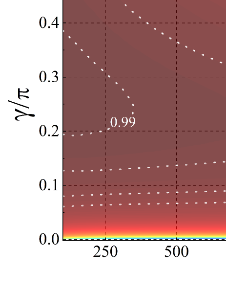
Figure 4: Transfer efficiency as functions of parameter $\gamma$ and operation time $t_{\rm{f}}$. Note the starting value of $\gamma$ is $0.001\pi$ since it can not be equal to zero.

The “chosen path” method in a real $\Lambda$-type system Wu et al. (2017) implies that if there is no decay from the excited state, perfect transfer efficiency can always be achieved regardless the choice of the parameter $\gamma$ and operation time $t_{\rm{f}}$. However, its efficiency can be very low if the strong decay in the excited state is considered. In Fig. 4, we also study the transfer efficiency as functions of the two parameters to see whether the robustness is still preserved in M-type system. In the calculations, the decay rates of molecule ⁸⁷Rb₂ are also taken into account. The detuning is fixed at $\Delta=2\pi{\rm{GHz}}$ and the parameter $\gamma$ starts at the value of $0.001\pi$ since it can not be equal to zero.

We can see from Fig. 4 that even in presence of strong decay from the intermediate states, nearly perfect transfer efficiency can be obtained in the M-type system within a wide range of the chosen parameters $\gamma$ and $t_{\rm{f}}$, which is quite opposite to the case when the “chosen path” method is applied in a real three-state system. The reason is the main population loss from the two excited states, $|2\rangle$ and $|4\rangle$, is firstly suppressed by the AE. Secondly, the excited state $|3\rangle$ in the generalized $\Lambda$-type system is actually a ground state with small decay rate. Therefore, the transient population in this state does not greatly influence the transfer efficiency.

In Fig. 4, we can also see that the property of the “chosen path” method is almost preserved in M-type system. The transfer efficiency is robust against the operation time $t_{\rm{f}}$ when the parameter $\gamma$ is fixed. Slight difference only lies in choosing the value of parameter $\gamma$ when the operation time $t_{\rm{f}}$ is fixed, which is $\gamma$ should not be too small in order for the perfect transfer efficiency. The reason is $\tilde{\Omega}_{\rm{EP}}$ and $\tilde{\Omega}_{\rm{ES}}$ tend to be very large at a small value of $\gamma$. Consequently, the AE condition is gradually broken down at the large value of $\tilde{\Omega}_{j}(j=1,2,3,4)$. The excited states $|2\rangle$ and $|4\rangle$ will be populated and the population will decay quickly out of the system, resulting in the decrease of the transfer efficiency.

Although Fig. 4 demonstrates that highly efficient creation of ultracold deeply-bound molecules under the C-STIRSAP with “chosen path” method can be completed in a very short time, it does not provide another information which we also concern very much. That is how strong the four modified Rabi frequencies $\tilde{\Omega}_{j}(j=1,2,3,4)$ will be under this protocol. Calculations reveal that the variations of the four Rabi frequencies $\tilde{\Omega}_{j}(j=1,2,3,4)$ under different choice of the operation time $t_{\rm{f}}$ are similar when the parameter $\gamma$ is fixed. Therefore, we can only investigate the amplitudes of $\tilde{\Omega}_{1}$ and $\tilde{\Omega}_{4}$ as a function of $t_{\rm{f}}$. This is because the amplitudes of $\tilde{\Omega}_{2}$ and $\tilde{\Omega}_{3}$ are always smaller than those of $\tilde{\Omega}_{1}$ and $\tilde{\Omega}_{4}$ (see the equation $\tilde{\Omega}_{1,4}=\sqrt{\tilde{\Omega}_{2}^{2}+\tilde{\Omega}_{3}^{2}}$). Here we set $\gamma=0.3\pi$ as an example and the result is shown by the red solid line in Fig. 5(a).

It is obvious from Fig. 5(a) that there is a trade-off between the pulse intensities and operation time. Shorter operation time of the C-STIRSAP requires stronger pulse intensities. On one hand, the pulse intensities can not be too strong in order to maintain the AE condition. On the other hand, the operation time can not be too long in order to avoid the population loss through the intermediate states. Hence, the two parameters should be chosen reasonably according to the actual situation. Besides, we point out that the pulse intensities can be further decreased by using a smaller detuning $\Delta$. This is because the four Rabi frequencies $\tilde{\Omega}_{j}(j=1,2,3,4)$ are proportional to the detuning, as can be found in Eqs. (64)-(66). The plots in Fig. 5(a) when the detuning is reduced to $\Delta=1.5\pi{\rm{GHz}}$ and $\Delta=1\pi{\rm{GHz}}$, respectively, verify our deduction. They clearly show the feasibility of the C-STIRSAP under the “chosen path” method that nearly perfect transfer efficiency can be obtained within a short operation time while the pulses do not have to be strong. For instance, we choose a point in this figure when $\Delta=1.5\pi{\rm{GHz}}$ and $t_{\rm{f}}=1000{\rm{ns}}$. The corresponding time sequence of the four Rabi frequencies in Fig. 5(b) and the population evolution of the M-type system in Fig. 5(c) demonstrate the high transfer efficiency while the amplitudes of $\tilde{\Omega}_{1}$ and $\tilde{\Omega}_{4}$ are just around $40\pi{\rm{MHz}}$.

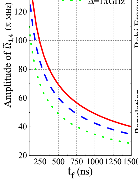
Figure 5: (a) Amplitudes of $\tilde{\Omega}_{1}$ and $\tilde{\Omega}_{4}$ as a function of the operation time $t_{\rm{f}}$ at different detuning. (b) and (c) present the time sequence of the four Rabi frequencies $\tilde{\Omega}_{j}(j=1,2,3,4)$ and the corresponding population transfer when the detuning and operation time are $\Delta=1.5\pi{\rm{GHz}}$ and $t_{\rm{f}}=1000{\rm{ns}}$, respectively. Note the parameter $\gamma$ is fixed at $0.3\pi$.

Finally, we discuss briefly the detection of ultracold deeply-bound molecules. High detection efficiency is important to test the created ultracold deeply-bound molecules, it is also critical for the preparation and characterization of novel many-body phases of dipolar molecules, such as crystalline bulk phases Büchler et al. (2007), exotic density order Schmidt et al. (2022), or spin order in optical lattices Gorshkov et al. (2011). Generally, we should first transfer the ultracold deeply-bound molecules back into the Feshbach molecules. Then we can detect them by using the standard absorption imaging. The back-transfer is usually realized by reversing the time sequence of the incident pulses for the creation process. Therefore, the detection efficiency critically depends on the creation efficiency of ultracold deeply-bound molecules. If the creation efficiency is $\chi$, then the detection efficiency will be $\chi^{2}$. Here, we directly give an example of the detection following the creation results in Figs. 5(b) and 5(c), which is presented in Fig. 6. In order to reverse the time sequence of the four Rabi frequencies $\tilde{\Omega}_{j}(j=1,2,3,4)$, the boundary condition of the parameter $\theta(t)$ is altered to be $\theta(0)=\pi/2$ and $\theta(t_{f})=\pi$. Therefore, $\theta(t)$ is redefined as

$$\theta(t)= \frac{\pi}{2}+\frac{\pi t}{2t_{f}}-\frac{1}{3}\sin(\frac{2\pi t}{t_{f}})+\frac{1}{24}\sin(\frac{4\pi t}{t_{f}}).$$ (83)

As a comparison, we also give the population evolution of the Feshbach state $|1\rangle$ in the ideal case of not considering the decay. We can clearly see in Fig. 6 that there is always a high detection efficiency under our C-STIRSAP protocol. The detection efficiency is about $95.16\%$, the result indicates a creation efficiency of about $97.55\%$. These results validate the potential of our approach for preserving the phase-space density of the ultracold mixture.

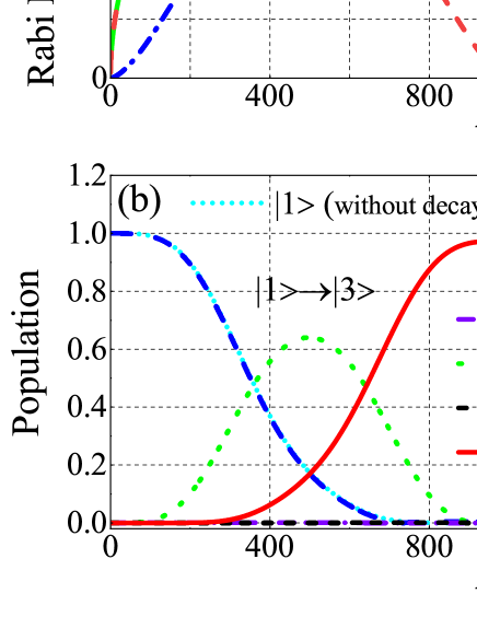
Figure 6: (a) Time sequence of the four Rabi frequencies $\tilde{\Omega}_{j}(j=1,2,3,4)$ for the creation and detection of ultracold deeply-bound molecules and (b) the corresponding population transfer. Population evolution of the Feshbach state $|1\rangle$ without considering the decay is also presented as a comparison. All parameters are the same as those in Fig. 5(b) and (c).

IV Conclusions

To conclude, we have proposed a scheme of C-STIRSAP in M-type system to create and detect ultracold deeply-bound molecules. The C-STIRSAP can speed up the population transfer without using strong pulses, resulting in the creation and detection with high efficiency. The key of our protocol is reducing the M-type structure into a generalized $\Lambda$-type system with the simplest resonant coupling, which principally allows us to employ all kinds of methods in the frame of STA to accelerate the adiabatic procedure. The simplification is realized under the assumption of AE together with a requirement of the relation among the four incident pulses. Examples of using the counter-diabatic driving and “chosen path” method verify the feasibility of the C-STIRSAP. Since the cost of STA is generally the precisely-controlled incident pulses, we note that the requirement of the relation among the four pulses in our C-STIRSAP protocol actually does not add extra complexity in experiments. In the end, we believe that our protocol is a good supplement to the arsenal of STA in multi-state quantum systems, which is of potential interest in applications where high-fidelity quantum control is essential (e.g., quantum information, atom optics and cavity QED).

References

- Blume (2012) D. Blume, Rep. Prog. Phys. 75, 046401 (2012).
- Hutson (2010) J. M. Hutson, Science 327, 788 (2010).
- Ulmanis et al. (2012) J. Ulmanis, J. Deiglmayr, M. Repp, R. Wester, and M. Weidemüller, Chem. Rev. 112, 4890 (2012).
- DeMille (2002) D. DeMille, Phys. Rev. Lett. 88, 067901 (2002).
- Carr et al. (2009) L. D. Carr, D. DeMille, R. V. Krems, and J. Ye, New J. Phys. 11, 055049 (2009).
- Mitra et al. (2022) D. Mitra, K. H. Leung, and T. Zelevinsky, Phys. Rev. A 105, 040101 (2022).
- Jones et al. (2006) K. M. Jones, E. Tiesinga, P. D. Lett, and P. S. Julienne, Rev. Mod. Phys. 78, 483 (2006).
- Král et al. (2007) P. Král, I. Thanopulos, and M. Shapiro, Rev. Mod. Phys. 79, 53 (2007).
- Winkler et al. (2007) K. Winkler, F. Lang, G. Thalhammer, P. v. d. Straten, R. Grimm, and J. H. Denschlag, Phys. Rev. Lett. 98, 043201 (2007).
- Thalhammer et al. (2006) G. Thalhammer, K. Winkler, F. Lang, S. Schmid, R. Grimm, and J. H. Denschlag, Phys. Rev. Lett. 96, 050402 (2006).
- Lang et al. (2008) F. Lang, K. Winkler, C. Strauss, R. Grimm, and J. Hecker Denschlag, Phys. Rev. Lett. 101, 133005 (2008).
- Danzl et al. (2008) J. G. Danzl, E. Haller, M. Gustavsson, M. J. Mark, R. Hart, N. Bouloufa, O. Dulieu, H. Ritsch, and H.-C. Nägerl, Science 321, 1062 (2008).
- Stellmer et al. (2012) S. Stellmer, B. Pasquiou, R. Grimm, and F. Schreck, Phys. Rev. Lett. 109, 115302 (2012).
- Polovy et al. (2020) G. Polovy, E. Frieling, D. Uhland, J. Schmidt, and K. W. Madison, Phys. Rev. A 102, 013310 (2020).
- Aikawa et al. (2010) K. Aikawa, D. Akamatsu, M. Hayashi, K. Oasa, J. Kobayashi, P. Naidon, T. Kishimoto, M. Ueda, and S. Inouye, Phys. Rev. Lett. 105, 203001 (2010).
- Ospelkaus et al. (2008) S. Ospelkaus, A. Pe’er, K.-K. Ni, J. J. Zirbel, B. Neyenhuis, S. Kotochigova, P. S. Julienne, J. Ye, and D. S. Jin, Nat. Phys. 4, 622 (2008).
- Ni et al. (2008) K.-K. Ni, S. Ospelkaus, M. H. G. de Miranda, A. Pe’er, B. Neyenhuis, J. J. Zirbel, S. Kotochigova, P. S. Julienne, D. S. Jin, and J. Ye, Science 322, 231 (2008).
- Molony et al. (2016) P. K. Molony, A. Kumar, P. D. Gregory, R. Kliese, T. Puppe, C. R. Le Sueur, J. Aldegunde, J. M. Hutson, and S. L. Cornish, Phys. Rev. A 94, 022507 (2016).
- Seeßelberg et al. (2018) F. Seeßelberg, N. Buchheim, Z.-K. Lu, T. Schneider, X.-Y. Luo, E. Tiemann, I. Bloch, and C. Gohle, Phys. Rev. A 97, 013405 (2018).
- Liu et al. (2019) L. Liu, D.-C. Zhang, H. Yang, Y.-X. Liu, J. Nan, J. Rui, B. Zhao, and J.-W. Pan, Phys. Rev. Lett. 122, 253201 (2019).
- Park et al. (2015) J. W. Park, S. A. Will, and M. W. Zwierlein, Phys. Rev. Lett. 114, 205302 (2015).
- Guo et al. (2016) M. Guo, B. Zhu, B. Lu, X. Ye, F. Wang, R. Vexiau, N. Bouloufa-Maafa, G. Quéméner, O. Dulieu, and D. Wang, Phys. Rev. Lett. 116, 205303 (2016).
- Rvachov et al. (2017) T. M. Rvachov, H. Son, A. T. Sommer, S. Ebadi, J. J. Park, M. W. Zwierlein, W. Ketterle, and A. O. Jamison, Phys. Rev. Lett. 119, 143001 (2017).
- Yang et al. (2020) A. Yang, S. Botsi, S. Kumar, S. B. Pal, M. M. Lam, I. Čepaitė, A. Laugharn, and K. Dieckmann, Phys. Rev. Lett. 124, 133203 (2020).
- Cairncross et al. (2021) W. B. Cairncross, J. T. Zhang, L. R. B. Picard, Y. Yu, K. Wang, and K.-K. Ni, Phys. Rev. Lett. 126, 123402 (2021).
- Stevenson et al. (2023) I. Stevenson, A. Z. Lam, N. Bigagli, C. Warner, W. Yuan, S. Zhang, and S. Will, Phys. Rev. Lett. 130, 113002 (2023).
- Lam et al. (2022) A. Z. Lam, N. Bigagli, C. Warner, W. Yuan, S. Zhang, E. Tiemann, I. Stevenson, and S. Will, Phys. Rev. Res. 4, L022019 (2022).
- Warner et al. (2023) C. Warner, N. Bigagli, A. Z. Lam, W. Yuan, S. Zhang, I. Stevenson, and S. Will, New J. Phys. 25, 053036 (2023).
- Voges et al. (2020) K. K. Voges, P. Gersema, M. Meyer zum Alten Borgloh, T. A. Schulze, T. Hartmann, A. Zenesini, and S. Ospelkaus, Phys. Rev. Lett. 125, 083401 (2020).
- Dou et al. (2012) F.-Q. Dou, S.-C. Li, H. Cao, and L.-B. Fu, Phys. Rev. A 85, 023629 (2012).
- Dou et al. (2013) F.-Q. Dou, L.-B. Fu, and J. Liu, Phys. Rev. A 87, 043631 (2013).
- Zhang and Dou (2021) J.-H. Zhang and F.-Q. Dou, New J. Phys. 23, 063001 (2021).
- Takekoshi et al. (2014) T. Takekoshi, L. Reichsöllner, A. Schindewolf, J. M. Hutson, C. R. Le Sueur, O. Dulieu, F. Ferlaino, R. Grimm, and H.-C. Nägerl, Phys. Rev. Lett. 113, 205301 (2014).
- Guéry-Odelin et al. (2019) D. Guéry-Odelin, A. Ruschhaupt, A. Kiely, E. Torrontegui, S. Martínez-Garaot, and J. G. Muga, Rev. Mod. Phys. 91, 045001 (2019).
- Demirplak and Rice (2003) M. Demirplak and S. A. Rice, J. Phys. Chem. A 107, 9937 (2003).
- Demirplak and Rice (2005) M. Demirplak and S. A. Rice, J. Phys. Chem. B 109, 6838 (2005).
- Demirplak and Rice (2008) M. Demirplak and S. A. Rice, J. Chem. Phys. 129, 154111 (2008).
- Berry (2009) M. V. Berry, J. Phys. A: Math. Theor. 42, 365303 (2009).
- Chen et al. (2010) X. Chen, I. Lizuain, A. Ruschhaupt, D. Guéry-Odelin, and J. G. Muga, Phys. Rev. Lett. 105, 123003 (2010).
- Masuda and Rice (2015) S. Masuda and S. A. Rice, J. Phys. Chem. A 119, 3479 (2015).
- Lewis and Riesenfeld (1969) H. R. Lewis and W. B. Riesenfeld, J. Math. Phys. 10, 1458 (1969).
- Chen et al. (2011) X. Chen, E. Torrontegui, and J. G. Muga, Phys. Rev. A 83, 062116 (2011).
- Chen and Muga (2012) X. Chen and J. G. Muga, Phys. Rev. A 86, 033405 (2012).
- Ho and Tseng (2015) C.-P. Ho and S.-Y. Tseng, Opt. Lett. 40, 4831 (2015).
- Lu et al. (2017) X.-J. Lu, M. Li, Z. Y. Zhao, C.-L. Zhang, H.-P. Han, Z.-B. Feng, and Y.-Q. Zhou, Phys. Rev. A 96, 023843 (2017).
- Ibáñez et al. (2012) S. Ibáñez, X. Chen, E. Torrontegui, J. G. Muga, and A. Ruschhaupt, Phys. Rev. Lett. 109, 100403 (2012).
- Song et al. (2016) X.-K. Song, Q. Ai, J. Qiu, and F.-G. Deng, Phys. Rev. A 93, 052324 (2016).
- Baksic et al. (2016) A. Baksic, H. Ribeiro, and A. A. Clerk, Phys. Rev. Lett. 116, 230503 (2016).
- Zhou et al. (2017) B. Zhou, A. Baksic, H. Ribeiro, C. Yale, F. Heremans, P. Jerger, A. Auer, G. Burkard, A. Clerk, and D. Awschalom, Nat. Phys. 13, 330 (2017).
- Wu et al. (2019) J.-L. Wu, Y. Wang, J. Song, Y. Xia, S.-L. Su, and Y.-Y. Jiang, Phys. Rev. A 100, 043413 (2019).
- Wu et al. (2017) J.-L. Wu, X. Ji, and S. Zhang, Opt. Express 25, 21084 (2017).
- Tang et al. (2022) S. Tang, J.-L. Wu, C. Lü, J. Song, and Y. Jiang, Phys. Rev. Appl. 18, 014038 (2022).
- Li and Chen (2016) Y.-C. Li and X. Chen, Phys. Rev. A 94, 063411 (2016).
- Du et al. (2016) Y.-X. Du, Z.-T. Liang, Y.-C. Li, X.-X. Yue, Q.-X. Lv, W. Huang, X. Chen, H. Yan, and S.-L. Zhu, Nat. Commun. 7, 12479 (2016).
- Stwalley (2004) W. C. Stwalley, Eur. Phys. J. D 31, 221 (2004).
- Danzl et al. (2010) J. G. Danzl, M. J. Mark, E. Haller, M. Gustavsson, R. Hart, J. Aldegunde, J. M. Hutson, and H.-C. Nägerl, Nat. Phys. 6, 265 (2010).
- Kuznetsova et al. (2008) E. Kuznetsova, P. Pellegrini, R. Côté, M. D. Lukin, and S. F. Yelin, Phys. Rev. A 78, 021402(R) (2008).
- Mackie and Phou (2010) M. Mackie and P. Phou, Phys. Rev. A 82, 011609(R) (2010).
- Malinovsky and Tannor (1997) V. S. Malinovsky and D. J. Tannor, Phys. Rev. A 56, 4929 (1997).
- Shore et al. (1991) B. W. Shore, K. Bergmann, J. Oreg, and S. Rosenwaks, Phys. Rev. A 44, 7442 (1991).
- Pillet et al. (1993) P. Pillet, C. Valentin, R.-L. Yuan, and J. Yu, Phys. Rev. A 48, 845 (1993).
- Oreg et al. (1985) J. Oreg, G. Hazak, and J. H. Eberly, Phys. Rev. A 32, 2776 (1985).
- Garraway and Suominen (1998) B. M. Garraway and K.-A. Suominen, Phys. Rev. Lett. 80, 932 (1998).
- Vitanov (2020) N. V. Vitanov, Phys. Rev. A 102, 023515 (2020).
- Torrontegui et al. (2013) E. Torrontegui, S. Ibáñez, S. Martínez-Garaot, M. Modugno, A. del Campo, D. Guéry-Odelin, A. Ruschhaupt, X. Chen, and J. G. Muga, Adv. At. Mol. Opt. Phys. 62, 117 (2013).
- Taras et al. (2021) A. K. Taras, A. Tuniz, M. A. Bajwa, V. Ng, J. M. Dawes, C. G. Poulton, and C. M. D. Sterke, Adv. Phys.: X 6, 1894978 (2021).
- Büchler et al. (2007) H. P. Büchler, E. Demler, M. Lukin, A. Micheli, N. Prokof’ev, G. Pupillo, and P. Zoller, Phys. Rev. Lett. 98, 060404 (2007).
- Schmidt et al. (2022) M. Schmidt, L. Lassablière, G. Quéméner, and T. Langen, Phys. Rev. Res. 4, 013235 (2022).
- Gorshkov et al. (2011) A. V. Gorshkov, S. R. Manmana, G. Chen, J. Ye, E. Demler, M. D. Lukin, and A. M. Rey, Phys. Rev. Lett. 107, 115301 (2011).