Locally Differentially Private Graph Embedding

Abstract

Graph embedding has been demonstrated to be a powerful tool for learning latent representations for nodes in a graph. However, despite its superior performance in various graph-based machine learning tasks, learning over graphs can raise significant privacy concerns when graph data involves sensitive information. To address this, in this paper, we investigate the problem of developing graph embedding algorithms that satisfy local differential privacy (LDP). We propose LDP-GE, a novel privacy-preserving graph embedding framework, to protect the privacy of node data. Specifically, we propose an LDP mechanism to obfuscate node data and adopt personalized PageRank as the proximity measure to learn node representations. Then, we theoretically analyze the privacy guarantees and utility of the LDP-GE framework. Extensive experiments conducted over several real-world graph datasets demonstrate that LDP-GE achieves favorable privacy-utility trade-offs and significantly outperforms existing approaches in both node classification and link prediction tasks.

I Introduction

Many types of real-world data can be naturally represented as graphs, such as social networks [1], financial networks [2], and transportation networks [3]. In the past few years, graph embedding has attracted much attention due to its superior performance in various machine learning tasks, such as node classification, link prediction, and graph reconstruction [4, 5, 6, 7]. Graph embedding is a representation learning problem that captures node features and structure information in a graph using vectors. However, most real-world graphs involve sensitive information about individuals and their activities, such as users’ profile information and comments in social networks. Releasing the embedding vectors of users gives malicious attackers a potential way to infer the attributes and social interactions, which could potentially be private to the user. The growing awareness of privacy and the establishment of regulations and laws indicate that it is important to develop privacy-preserving graph embedding algorithms.

Differential privacy (DP) [8] has recently become the dominant paradigm for safeguarding individual privacy in data analysis. A vast majority of differentially private graph learning algorithms are designed under the centralized model [9, 10, 11, 12, 13, 14], which assumes that a trusted data curator holds the personal data of all users and releases sanitized versions of statistics or machine learning models. However, this assumption is impractical in some applications due to security or logistical reasons. The centralized model carries the risk of users’ data being breached by the trusted data curator through illegal access or internal fraud [15, 16]. In addition, some social networks are inherently decentralized and distributed [17], where no centralized party holds the entire social graph. As a result, the centralized DP algorithms cannot be applied to these decentralized social networks.

In contrast to centralized DP, local differential privacy (LDP) [18] has emerged as a promising approach that ensures stronger privacy guarantees for users in scenarios involving data aggregation. LDP operates under a local model, where each user perturbs their data locally and transmits only the perturbed data to an untrusted data curator. This means that the original personal data remains confined to the users’ local devices, effectively eliminating the risk of data leakage that might occur in the centralized DP settings. As a result, LDP provides an enhanced level of privacy protection for individuals. The practicality and effectiveness of LDP have been recognized by major technology companies, including Google [19], Apple [20], and Microsoft [21], which have deployed LDP-based solutions to handle sensitive user data while preserving privacy. Moreover, the applicability of LDP extends beyond centralized settings, making it an appealing choice for decentralized applications.

In this paper, our focus is on exploring the design of graph embedding algorithms that satisfy LDP, where the node features are private and sensitive, and the global graph structure information is maintained by the data curator. This scenario arises in various domains, particularly in social network analysis and mobile computing. For instance, consider a social networking platform or a dating application that utilizes node representations to capture relationships between users. In this context, individuals’ attributes and preferences are treated as private node features. Integrating LDP in graph embedding for such applications can safeguard users’ sensitive data while empowering the platform to offer valuable services.

In the local setting for DP, each user sends only perturbed node features to the data collector. However, a key challenge arises when dealing with high-dimensional node features used for graph embedding, as the perturbation in such scenarios can result in significant information loss. To overcome this challenge, some researchers have proposed various approaches, including sampling techniques and tailored perturbation mechanisms, aimed at preserving utility in the high-dimensional space [22, 23, 24, 25, 26]. Nevertheless, these mechanisms also introduce excessive noise to the data, potentially compromising overall performance.

In this paper, we propose the Locally Differentially Private Graph Embedding framework (LDP-GE), a novel privacy-preserving graph embedding framework based on private node data. Our framework offers provable privacy guarantees, building on the principles of local differential privacy. Specifically, to protect the privacy of node features, we propose the HDS (an acronym for High-Dimensional Square wave) mechanism, an LDP perturbation technique tailored for high-dimensional data. Each user can adopt this perturbation mechanism to obfuscate their features before sending them to the data curator. The server leverages graph structure information and perturbed node features to learn graph representations. To avoid neighborhood explosion and over-smoothing issues, we decouple the feature transformation from the graph propagation. Furthermore, we adopt personalized PageRank as the proximity measure to learn node representations. Importantly, we conduct a comprehensive theoretical analysis of the utility of the LDP-GE framework. Our findings indicate that the proposed approach yields smaller error bounds than existing mechanisms, specifically, from $\mathcal{O}(\frac{d\log(d/\delta)}{\epsilon})$ down to $\mathcal{O}(\log(d/\delta)$), making it a more efficient solution. Finally, to assess the effectiveness of the LDP-GE framework, we conduct extensive experiments on various real-world datasets. The results demonstrate that our proposed method establishes state-of-the-art performance and achieves decent privacy-utility trade-offs in node classification and link prediction tasks. In summary, we highlight the main contributions as follows:

• We propose LDP-GE, an innovative framework designed to preserve privacy in graph embedding. Our approach can provide provable privacy guarantees while ensuring effective graph representation learning.

• To address the challenge dealing with high-dimensional node features, we propose the HDS mechanism to protect node feature privacy. This perturbation technique empowers users to obfuscate their features locally before reporting them to the data curator, thus enhancing privacy protection.

• We conduct a comprehensive theoretical analysis of the utility of the LDP-GE framework and alternative mechanisms. The results demonstrate that our algorithm offers smaller error bounds than existing mechanisms, reducing them from $\mathcal{O}(\frac{d\log(d/\delta)}{\epsilon})$ to $\mathcal{O}(\log(d/\delta)$).

• We conduct extensive experiments on various real-world datasets. The experimental results demonstrate that our proposed approach achieves better privacy-utility trade-offs than existing solutions. For instance, our proposed method achieves about 8% higher accuracy than the best competitor on the Pubmed dataset in node classification.

Organization. The rest of this paper is organized as follows. In Section II, we formally define the problem and provide the necessary background. Section III presents our locally differentially private graph embedding algorithm. The experimental results are shown in Section IV. Finally, we review the related literature and conclude this paper in Section V and Section VI, respectively.

II Preliminaries

In this section, we first introduce the problem definition and the concept of local differential privacy and then revisit some necessary background on graph embedding.

Problem Statement. We consider an undirected and unweighted graph $\mathcal{G}=(\mathcal{V},\mathcal{E})$, where $\mathcal{V}$ is the set of nodes (i.e., users) and $\mathcal{E}$ represents the set of edges. Let $|\mathcal{V}|$ be the number of nodes. Each user $v\in\mathcal{V}$ is characterized by a $d$-dimensional feature vector $\mathbf{x}_{v}$, and we use $\mathbf{X}\in\mathbb{R}^{|\mathcal{V}|\times d}$ to denote the feature matrix. Without loss of generality, we assume the node features are normalized into $[-1,1]$. Let $\mathbf{A}$ and $\mathbf{D}$ represent the adjacency matrix and the diagonal degree matrix, respectively. For each node $v\in\mathcal{V}$, $\mathcal{N}(v)$ is the set of neighbors of $v$, and the degree of $v$ is $|\mathcal{N}(v)|$.

Now we assume that the data curator is an untrusted party and that it has access to the set of nodes $\mathcal{V}$ and edges $\mathcal{E}$. However, the data curator cannot observe feature matrix $\mathbf{X}$, which is private to the users. Our ultimate target is to learn a node embedding matrix while protecting the privacy of node data.

Local Differential Privacy. Differential privacy (DP) [8] has emerged as the de facto standard for protecting user privacy from attackers with arbitrary background knowledge. DP can be categorized into centralized DP and LDP (Local DP) [18]. Centralized DP assumes a scenario where a trusted curator holds all users’ personal data and releases sanitized versions of the statistics. In contrast to centralized DP, LDP operates under the assumption of a local model, where the data curator is considered untrusted. Specifically, each user perturbs their data using a randomized perturbation algorithm and sends the obfuscated data to the untrusted data curator. The individual perturbed data lacks inherent meaning, but it acquires significance for data analytics when aggregated. The formal definition of LDP is as follows:

Definition 1 ($\epsilon$-Local Differential Privacy).

Given $\epsilon>0$, a randomized algorithm $\mathcal{A}$ satisfies $\epsilon$-local differential privacy if and only if for any two users’ private data $x$ and $x^{\prime}$, and for any possible output $y\in Range(\mathcal{A})$, we have

$$\operatorname{Pr}[\mathcal{A}(x)=y]\leq e^{\epsilon}\cdot\operatorname{Pr}[\mathcal{A}(x^{\prime})=y].$$ (1)

Here, the parameter $\epsilon$ is called the privacy budget, which controls the strength of privacy protection: a lower privacy budget indicates stronger privacy preservation but leads to lower utility. According to the above definition, LDP guarantees that an attacker observing the output of the randomized algorithm cannot infer with high confidence whether the data source is $x$ or $x^{\prime}$ (controlled by the parameter $\epsilon$), regardless of the background information available to the attacker. Furthermore, LDP satisfies some important properties that can help us design complex algorithms.

Proposition 1 (Sequential Composition[27]).

Given the sequence of computations $\mathcal{A}_{1},\mathcal{A}_{2},\dots,\mathcal{A}_{k}$, if each $\mathcal{A}_{i}$ satisfies $\epsilon_{i}$-LDP, then their sequential execution on the same dataset satisfies $\sum_{i}\epsilon_{i}$-LDP.

Proposition 2 (Post-processing[27]).

Given $\mathcal{A}(\cdot)$ that satisfies $\epsilon$-LDP, then for any algorithm $\mathcal{B}$, the composed algorithm $\mathcal{B}(\mathcal{A}(\cdot))$ satisfies $\epsilon$-LDP.

Graph Embedding. The task of graph embedding is to learn a latent representation for each node. Extensive research works have shown that the latent representations can capture the structure and inherent properties of the graph, which can facilitate widespread downstream inference tasks, such as node classification and link prediction [4, 5, 6].

An important class of graph embedding methods are those that utilize the message passing algorithms [28], which have garnered significant attention due to their flexibility and good performance. Specifically, the message passing framework consists of two phases: (i) messages are propagated along the neighbors, and (ii) the messages are aggregated to obtain the updated representations. Most Graph Neural Networks, such as Graph Convolutional Network (GCN) [29] and Graph Attention Network (GAT) [30], employ the message passing procedure to spread information throughout the graph. At each layer, feature transformation is coupled with aggregation/propagation among neighbors. By increasing the number of layers, the model can incorporate information from more distant neighbors, thus facilitating more comprehensive learning of node representations. However, this can result in over-smoothing and neighborhood explosion [31, 32].

To tackle these issues, some studies [33, 34, 32, 35, 36] decouple the feature transformation from the graph aggregation/propagation and exploit node proximity queries to incorporate multi-hop neighborhood information. Personalized PageRank [37] is a widely-used proximity measure that can characterize node distances and similarities. Consequently, we apply the personalized PageRank matrix to the feature matrix $\mathbf{X}$ to obtain representation matrix $\mathbf{Z}$. Specifically, we consider the following graph propagation equation:

$$\mathbf{Z}=\mathbf{\Pi}\cdot\mathbf{X}=\sum\limits_{\ell=0}^{\infty}\alpha(1-\alpha)^{\ell}\cdot(\mathbf{D}^{r-1}\mathbf{A}\mathbf{D}^{-r})^{\ell}\cdot\mathbf{X}\,,$$ (2)

where $\mathbf{\Pi}$ is the personalized PageRank matrix, $r\in[0,1]$ is the convolution coefficient and $\alpha\in(0,1)$ is the decay factor. The parameter $\alpha$ controls the amount of information we capture from the neighborhood. To be specific, for the values of $\alpha$ closer to $1$, we place more emphasis on the immediate neighborhood of the node, which can avoid over-smoothing. As the value of $\alpha$ decreases to $0$, we instead give more attention to the multi-hop neighborhood of the node.

Notational Conventions. Throughout the paper, we use bold letters and capital bold letters to represent vectors and matrices, respectively. For instance, $\mathbf{x}=[x_{1},x_{2},\dots,x_{d}]^{\top}$ is the feature vector, and $\mathbf{X}$ is the feature matrix. The notation associated with a tilde, such as $\tilde{\mathbf{x}}$, denotes the value after LDP perturbation. Table I summarizes the frequently used mathematical notations in this paper.

TABLE I: Notations

Symbol	Description
$|\mathcal{V}|$	the number of nodes
$\mathbf{A}$, $\mathbf{D}$	the adjacency matrix and degree matrix
$\mathcal{N}(v)$, $|\mathcal{N}(v)|$	the neighbor set and the degree of node $v$
$\mathbf{x}_{v}$, $\tilde{\mathbf{x}}_{v}$	the feature vector and perturbed feature vector of node $v$
$d$, $k$	the number of dimensions and sampled dimensions
$\mathbf{X}$, $\mathbf{Z}$	the feature matrix and embedding matrix
$\alpha$, $r$	the decay factor and the convolution coefficient
$\mathbf{\Pi}$	the personalized PageRank matrix
$\mathbf{R}$, $\mathbf{Q}$	the residue matrix and reserve matrix
$\epsilon$	the privacy budget
$\mathbb{E}[x]$, $\operatorname{Var}[x]$	the expected value and variance of the random variable $x$

III The Proposed Method

In this section, we describe our proposed framework for graph embedding. The framework comprises two components: a perturbation module and a propagation module. The perturbation module is utilized to obfuscate node features before sending them to the data curator. This component helps relieve users’ concerns about sharing their private information and keep it confidential during uploading. However, the node features to be collected are likely high-dimensional, whereas most LDP perturbation functions focus on one-dimensional data, such as the Laplace mechanism. Since each user is authorized a limited privacy budget, the allocated privacy budget in each dimension is diluted as the number of dimensions increases, which results in more noise injection. Even though some LDP mechanisms, such as One-bit mechanism [21] and Piecewise mechanism [23], have been extended to handle the high-dimensional data [24, 23], these mechanisms introduce a significant amount of noise to the data that can compromise the performance. Square wave mechanism [38] is another LDP mechanism designed to reconstruct the distribution of one-dimensional numerical attributes. And this mechanism provides more concentrated perturbation than both mechanisms mentioned above (i.e., One-bit mechanism and Piecewise mechanism). Therefore, to tackle this issue, we develop an LDP mechanism HDS by non-trivially extending the Square wave mechanism to high-dimensional data.

The propagation module is used to propagate node features through exchanging information among adjacent nodes, and each node is updated based on the aggregation of its neighbors’ features. Most graph embedding methods suffer from neighborhood explosion and over-smoothing issues, as explained in Section II. To address these problems, we decouple feature transformation and propagation and adopt personalized PageRank as the graph propagation formula to obtain the representation matrix. More importantly, we conduct a theoretical analysis of the utility of graph embedding based on private node data.

In the rest of this section, we first introduce the technical details of the perturbation module used for privacy assurances and some theoretical properties of our proposed mechanism. Next, we present the propagation process designed for graph embedding. Finally, we conduct a comprehensive utility analysis of the proposed framework.

III-A Perturbation Module

The target of the perturbation module is to gather node features from individuals under LDP. In specific, each user $v\in\mathcal{V}$ perturbs his/her private feature vector $\mathbf{x}_{v}$ using the perturbation mechanism and sends the perturbed data $\tilde{\mathbf{x}}_{v}$ to the data curator. The crucial aspect is to devise a randomization mechanism that provides plausible deniability. In this section, we first review three existing perturbation mechanisms and discuss their deficiencies. Then, we propose our mechanism for feature perturbation.

Existing Solutions. Laplace mechanism, introduced by Dwork et al. [8], is a well-established approach enforcing differential privacy. It can be applied to the LDP setting in the following manner. Assuming each user possesses a one-dimensional value $x$ in the range of $[-1,1]$, we define a randomized function that generates a perturbed value $\tilde{x}=x+Lap(2/\epsilon)$. Here, $Lap(\lambda)$ represents a random variable that follows a Laplace distribution with a scale parameter $\lambda$. The Laplace distribution is characterized by the probability density function $f(x)=\frac{1}{2\lambda}\exp(-\frac{|x|}{\lambda})$.

To extend this mechanism to high-dimensional values, a straightforward method is to collect the perturbed value separately using the Laplace mechanism in each dimension. In this approach, each dimension is assigned a privacy budget of $\epsilon/d$. Applying the composition property of LDP as described in Proposition 1, we can conclude that the entire collection of values satisfies $\epsilon$-LDP. In the high-dimensional space, since the injected Laplace noise in each dimension follows $Lap(2d/\epsilon)$, it is evident that the perturbed value $\tilde{x}$ is unbiased, and its variance is $\frac{8d^{2}}{\epsilon^{2}}$. Furthermore, the Laplace mechanism embodies a category of LDP mechanisms known as unbounded mechanisms [39], where the noise injected into the original value ranges from negative to positive infinity.

In the one-dimensional Piecewise mechanism [23], the input domain is $[-1,1]$, and the range of perturbed data is $[-s,s]$, where $s=\frac{e^{\epsilon/2}+1}{e^{\epsilon/2}-1}$. Given an original value $x\in[-1,1]$, the perturbed value $\tilde{x}$ is sampled from the following distribution:

$$\operatorname{Pr}[\tilde{x}=c|x]=\left\{\begin{array}[]{ l l }p,&\text{if}\ c\in[\ell(x),r(x)]\\ \frac{p}{e^{\epsilon}},&\text{if}\ c\in[-s,\ell(x))\cup(r(x),s]\end{array}\right.,$$ (3)

where

$$p=\frac{e^{\epsilon}-e^{\epsilon/2}}{2e^{\epsilon/2}+2},$$

$$\ell(x)=\frac{s+1}{2}\cdot x-\frac{s-1}{2},\text{ and}$$

$$r(x)=\ell(x)+s-1.$$

Wang et al. [23] also propose an extension of the Piecewise mechanism to process high-dimensional data. The extended mechanism adopts a sampling technique so that each user reports only $k$ out of $d$ dimensions of his/her perturbed data to the data curator. In that case, each reporting dimension is allocated $\epsilon/k$ privacy budget, and the reporting data $\hat{x}$ is calibrated to ensure that the final outcome $\tilde{x}$ is unbiased. Formally, $\tilde{x}$ is obtained as follows:

$$\tilde{x}=\frac{d}{k}\cdot\hat{x}.$$ (4)

Meanwhile, in the high-dimensional setting, the variance of ${x}$ induced by Piecewise mechanism is

$$\operatorname{Var}[\tilde{x}]=\frac{d(e^{\epsilon/(2k)}+3)}{3k(e^{\epsilon/(2k)}-1)^{2}}+[\frac{d\cdot e^{\epsilon/(2k)}}{k(e^{\epsilon/(2k)}-1)}-1]\cdot x^{2}.$$ (5)

Multi-bit mechanism [24] is another perturbation function used to handle high-dimensional data under LDP. In its one-dimensional form, the original data $x\in[-1,1]$ is perturbed into $-1$ or $1$, with the following probabilities:

$$\operatorname{Pr}[\tilde{x}=c|x]=\left\{\begin{array}[]{ l l }\frac{1}{e^{\epsilon}+1}+\frac{x+1}{2}\cdot\frac{e^{\epsilon}-1}{e^{\epsilon}+1},&\text{if}\ c=1\\ \frac{e^{\epsilon}}{e^{\epsilon}+1}-\frac{x+1}{2}\cdot\frac{e^{\epsilon}-1}{e^{\epsilon}+1},&\text{if}\ c=-1\end{array}\right..$$ (6)

Similar to the Piecewise mechanism, in the high-dimensional space, the algorithm first uniformly samples $k$ out of $d$ dimensions without replacement and then performs $\frac{\epsilon}{k}$-LDP perturbation for each sampled dimension. In the end, the data curator transforms the reporting data $\hat{x}$ to its unbiased estimate

$$\tilde{x}=\frac{d}{k}\cdot\frac{e^{\epsilon/k}+1}{e^{\epsilon/k}-1}\cdot\hat{x}.$$ (7)

The variance of $\tilde{x}$ induced by Multi-bit mechanism is

$$\operatorname{Var}[\tilde{x}]=\frac{d}{k}\cdot(\frac{e^{\epsilon/k}+1}{e^{\epsilon/k}-1})^{2}-x^{2}.$$ (8)

In contrast to the Laplace mechanism, the Piecewise and Multi-bit mechanisms perturb the original value into a bounded domain. Consequently, these mechanisms are referred to as bounded mechanisms.

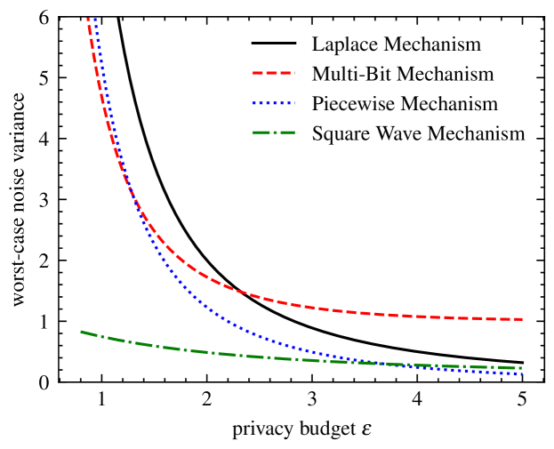
Figure 1: The worst-case noise variance vs. privacy budget for one-dimensional data.

Deficiencies of Existing Solutions. Even though these mechanisms can handle high-dimensional data, they introduce a significant amount of noise to the private data, leading to a decline in performance. To be specific, in the one-dimensional scenario, we visualize the worst-case noise variance of different mechanisms under varying privacy budgets, as illustrated in Figure 1. Note that in Figure 1, we also add the Square wave mechanism [38] for comparison. The Square wave mechanism was originally proposed in [38], which can achieve LDP when handling one-dimensional data. We can observe that the Square wave mechanism [38] provides a considerably smaller noise variance than the Piecewise mechanism for $\epsilon\leq 3.5$, and only slightly larger than the latter for $\epsilon>3.5$. Moreover, the worst-case noise variance provided by the Square wave mechanism is consistently smaller than that of the Laplace mechanism and the Multi-bit mechanism when $\epsilon\leq 5.0$. In consequence, the Square wave mechanism provides more concentrated perturbation. In high-dimensional settings, unbiased calibration is not conducive to graph embedding and can result in injecting excessive noise. The Square wave mechanism is designed to estimate the distribution of one-dimensional numerical data. Hence, inspired by the ideas of [23] and [24], we generalize the Square wave mechanism to feature collection in high-dimensional space.

HDS Mechanism. Our HDS mechanism is built upon the Square wave mechanism [38], which can handle only one-dimensional data. The Square wave mechanism is based on the following intuition. Given a single feature $x$, the perturbation module should report a value close to $x$ with a higher probability than a value far away from $x$. To some extent, the value close to $x$ also carries useful information about the input. The Square wave mechanism is initially designed for an input domain of $[0,1]$. However, in our scenario, the node features are normalized to the range of $[-1,1]$. Consequently, we extend this mechanism to enhance its capability in handling a broader range of node features, specifically $[-1,1]$. Algorithm 1 outlines the perturbation process for one-dimensional data. The algorithm takes a single feature $x\in[-1,1]$ as input and produces a perturbed feature $\tilde{x}\in[-b-1,1+b]$, where $b=\frac{\epsilon e^{\epsilon}-e^{\epsilon}+1}{e^{\epsilon}(e^{\epsilon}-\epsilon-1)}.$ The noisy output $\tilde{x}$ follows the distribution as below:

$$\operatorname{Pr}[\tilde{x}=c|x]=\left\{\begin{array}[]{ l l }p,&\text{if}\ c\in[x-b,x+b]\\ q,&\text{if}\ c\in[-b-1,x-b)\cup(x+b,1+b]\end{array}\right.,$$ (9)

where

$$p=\frac{e^{\epsilon}}{2be^{\epsilon}+2}\,,\quad q=\frac{1}{2be^{\epsilon}+2}\,.$$

Input: single feature $x\in[-1,1]$, privacy budget $\epsilon>0$

Output: perturbed feature $\tilde{x}\in[-b-1,1+b]$

1 Let $b=\frac{\epsilon e^{\epsilon}-e^{\epsilon}+1}{e^{\epsilon}(e^{\epsilon}-\epsilon-1)}$;

2 Let $\eta$ be sampled uniformly from $[0,1]$;

3 if $\eta<\frac{be^{\epsilon}}{be^{\epsilon}+1}$ then

4       Sample a random value $\tilde{x}$ uniformly from $[x-b,x+b]$;

5      

6else

7       Sample a random value $\tilde{x}$ uniformly from $[-b-1,x-b)\cup(x+b,1+b]$;

8      

return $\tilde{x}$

Algorithm 1 Extended Square Wave Mechanism

Algorithm 2 presents the pseudo-code of our HDS mechanism for high-dimensional feature collection. The algorithm requires that each user perturbs only $k$ dimensions of their features vector rather than $d$. This is because, according to the composition property of LDP described in Proposition 1, it increases the privacy budget for each dimension from $\epsilon/d$ to $\epsilon/k$, reducing the noise variance. Given a feature vector $\mathbf{x}$, the algorithm first uniformly samples $k$ values from $\{1,2,\dots,d\}$ without replacement, where $k$ is a parameter that controls the number of dimensions to be perturbed. Then for each sampled value $j$, the perturbed feature $\tilde{x}_{j}$ is generated by Algorithm 1, taking $x_{j}$ and $\frac{\epsilon}{k}$ as input. Correspondingly, the rest of the $d-k$ features are encoded into $0$ to prevent privacy leakage. Given that the output domain of the HDS mechanism is bounded, our proposed mechanism can be categorized as a bounded mechanism.

Theoretical Properties. The HDS mechanism provides the following assurances.

Firstly, the ensuing theorem establishes the privacy guarantee of our proposed mechanism.

Theorem 1.

The HDS mechanism presented in Algorithm 2 satisfies $\epsilon$-local differential privacy for each node.

Proof.

First, we prove that the Algorithm 1 provides $\epsilon$-LDP. Let $\mathcal{A}(x)$ be the Algorithm 1 that takes as input the single feature $x$, and $\tilde{x}=\mathcal{A}(x)$ is the obfuscated feature corresponding to $x$. Suppose $x_{1}$ and $x_{2}$ are private features of any two users. According to Equation (9), for any output $\tilde{x}\in[-b-1,1+b]$, we have

$$\frac{\operatorname{Pr}[\mathcal{A}(x_{1})=\tilde{x}]}{\operatorname{Pr}[\mathcal{A}(x_{2})=\tilde{x}]}\leq\frac{\frac{e^{\epsilon}}{2be^{\epsilon}+2}}{\frac{1}{2be^{\epsilon}+2}}=e^{\epsilon}.$$

Thus, the Algorithm 1 satisfies $\epsilon$-LDP. Since Algorithm 2 executes $\frac{\epsilon}{k}$-LDP operations (Algorithm 1) $k$ times on the same input data, then according to the composition property, Algorithm 2 satisfies $\epsilon$-local differential privacy. ∎

Input: feature vector $\mathbf{x}\in[-1,1]^{d}$, privacy budget $\epsilon>0$, sampling parameter $k\in\{1,2,...,d\}$

Output: perturbed feature vector $\tilde{\mathbf{x}}\in[-b-1,1+b]^{d}$

1 Let $\mathcal{S}$ be a set of $k$ values sampled uniformly without replacement from $\{1,2,\dots,d\}$;

2 for $j\in\{1,2,\dots,d\}$ do

3       if $j\in\mathcal{S}$ then

4             $\tilde{x}_{j}\leftarrow$ Feed $x_{j}$ and $\frac{\epsilon}{k}$ as input to Algorithm 1;

5            

6      else

7             $\tilde{x}_{j}\leftarrow 0$;

8      

return $\tilde{\mathbf{x}}=[\tilde{x}_{1},\tilde{x}_{2},\dots,\tilde{x}_{d}]^{\top}$

Algorithm 2 HDS Mechanism

In the following analysis, we examine the bias and variance of the HDS mechanism.

Lemma 1.

Let $\tilde{\mathbf{x}}_{v}$ denote the output of the Algorithm 2 on the input vector $\mathbf{x}_{v}$. For any dimension $j\in\{1,2,\dots,d\}$, we have

$$\mathbb{E}[\tilde{x}_{v,j}]=C\cdot x_{v,j}$$ (10)

and

$$\operatorname{Var}[\tilde{x}_{v,j}]=\frac{k}{d}\cdot\frac{b^{3}e^{\epsilon/k}+3b^{2}+3b+1}{3(be^{\epsilon/k}+1)}+(C-C^{2})\cdot x_{v,j}^{2}\,,$$ (11)

where $C=\frac{k}{d}\cdot\frac{b(e^{\epsilon/k}-1)}{be^{\epsilon/k}+1}$.

Proof.

For the expectation, we have

$$\mathbb{E}[\tilde{x}_{v,j}] =\mathbb{E}[\tilde{x}_{v,j}|j\in\mathcal{S}]\operatorname{Pr}[j\in\mathcal{S}]+\mathbb{E}[\tilde{x}_{v,j}|j\notin\mathcal{S}]\operatorname{Pr}[j\notin\mathcal{S}]$$

$$=\frac{k}{d}\cdot\mathbb{E}[\tilde{x}_{v,j}|j\in\mathcal{S}].$$ (12)

According to Equation (9), we have

$$\mathbb{E}[\tilde{x}_{v,j}|j\in\mathcal{S}]= \ \frac{1}{2be^{\epsilon/k}+2}\cdot(\int_{-1-b}^{x_{v,j}-b}t\,dt$$

$$+\int_{x_{v,j}-b}^{x_{v,j}+b}te^{\epsilon/k}\,dt+\int_{x_{v,j}+b}^{1+b}t\,dt)$$

$$= \ \frac{b(e^{\epsilon/k}-1)}{be^{\epsilon/k}+1}\cdot x_{v,j}.$$ (13)

Combining (III-A) and (III-A) we conclude

$$\mathbb{E}[\tilde{x}_{v,j}]=\frac{k}{d}\cdot\frac{b(e^{\epsilon/k}-1)}{be^{\epsilon/k}+1}\cdot x_{v,j}=C\cdot x_{v,j}.$$ (14)

For the variance, we have

$$\operatorname{Var}[\tilde{x}_{v,j}]= \ \mathbb{E}[\tilde{x}_{v,j}^{2}]-(\mathbb{E}[\tilde{x}_{v,j}])^{2}$$

$$= \ \mathbb{E}[\tilde{x}_{v,j}^{2}|j\in\mathcal{S}]\operatorname{Pr}[j\in\mathcal{S}]$$

$$\,+\mathbb{E}[\tilde{x}_{v,j}^{2}|j\notin\mathcal{S}]\operatorname{Pr}[j\notin\mathcal{S}]-(\mathbb{E}[\tilde{x}_{v,j}])^{2}$$

$$= \ \frac{k}{d}\cdot\mathbb{E}[\tilde{x}_{v,j}^{2}|j\in\mathcal{S}]-(\mathbb{E}[\tilde{x}_{v,j}])^{2}.$$ (15)

According to Equation (9), we have

$$\mathbb{E}[\tilde{x}_{v,j}^{2}|j\in\mathcal{S}]=\frac{1}{2be^{\epsilon/k}+2}\cdot(\int_{-1-b}^{x_{v,j}-b}t^{2}\,dt$$

$$\ +\int_{x_{v,j}-b}^{x_{v,j}+b}t^{2}e^{\epsilon/k}\,dt+\int_{x_{v,j}+b}^{1+b}t^{2}\,dt)$$

$$= \ \frac{b^{3}e^{\epsilon/k}+3b^{2}+3b+1}{3(be^{\epsilon/k}+1)}+\frac{b(e^{\epsilon/k}-1)}{be^{\epsilon/k}+1}\cdot x_{v,j}^{2}.$$ (16)

Combining (14), (III-A) and (III-A) yields

$$\operatorname{Var}[\tilde{x}_{v,j}]=\ \frac{k(b^{3}e^{\epsilon/k}+3b^{2}+3b+1)}{3d(be^{\epsilon/k}+1)}+(C-C^{2})x_{v,j}^{2}.$$

∎

III-B Propagation Module

Input: graph $\mathcal{G}=(\mathcal{V},\mathcal{E})$, perturbed feature matrix $\tilde{\mathbf{X}}$, decay factor $\alpha$, convolutional coefficient $r$, threshold $r_{max}$

Output: embedding matrix $\tilde{\mathbf{Z}}$

1 Initialize reserve matrix $\mathbf{Q}\leftarrow\mathbf{0}$ and residue matrix $\mathbf{R}\leftarrow\mathbf{D}^{-r}\tilde{\mathbf{X}}$;

2 while $\exists v$ and $\exists j\in\{0,\dots,d-1\}$ s.t. $|\mathbf{R}(v,j)|>r_{max}$ do

3       for $u\in\mathcal{N}(v)$ do

4             $\mathbf{R}(u,j)\leftarrow\mathbf{R}(u,j)+(1-\alpha)\cdot\frac{\mathbf{R}(v,j)}{|\mathcal{N}(u)|}$;

5            

6      $\mathbf{Q}(v,j)\leftarrow\mathbf{Q}(v,j)+\alpha\cdot\mathbf{R}(v,j)$ ;

7       $\mathbf{R}(v,j)\leftarrow 0$ ;

8      

9$\tilde{\mathbf{Z}}\leftarrow\mathbf{D}^{r}\cdot\mathbf{Q}$;

return $\tilde{\mathbf{Z}}$

Algorithm 3 Backward Push Propagation

The propagation module takes as input the perturbed feature matrix $\tilde{\mathbf{X}}$, which comprises obfuscated feature vectors $\tilde{\mathbf{x}}_{v}$ for each user $v\in\mathcal{V}$, and outputs the embedding matrix $\tilde{\mathbf{Z}}$. To incorporate neighborhood information, we exploit personalized PageRank as the proximity measure for graph propagation. Formally, the process of graph propagation can be formulated as follows:

$$\tilde{\mathbf{Z}}=\mathbf{\Pi}\cdot\tilde{\mathbf{X}}=\sum\limits_{\ell=0}^{\infty}\alpha(1-\alpha)^{\ell}\cdot(\mathbf{D}^{r-1}\mathbf{A}\mathbf{D}^{-r})^{\ell}\cdot\tilde{\mathbf{X}}\,.$$ (17)

We utilize the well-established backward push algorithm [4] as a standard technique to calculate personalized PageRank. In our work, we extend this algorithm to enable efficient graph propagation.

Algorithm 3 illustrates the pseudo-code of the backward push propagation algorithm. Intuitively, the algorithm starts by setting the residue matrix $\mathbf{R}=\mathbf{D}^{-r}\mathbf{A}$ and the reserve matrix $\mathbf{Q}=\mathbf{0}$ (Line 1). Subsequently, a push procedure (Line 2-6) is executed for each node $v$ if the absolute value of the residue entry $\mathbf{R}(v,j)$ exceeds a threshold $r_{max}$ until no such $v$ exists. Specifically, if there is a node $v$ meeting $|\mathbf{R}(v,j)|>r_{max}$, the algorithm increases the residue of each neighbor $u$ by $(1-\alpha)\cdot\frac{\mathbf{R}(v,j)}{|\mathcal{N}(u)|}$ and increases the reserve of node $v$ by $\alpha\times\mathbf{R}(v,j)$. After that, it reset the residue $\mathbf{R}(v,j)$ to $0$. Finally, the embedding matrix is $\tilde{\mathbf{Z}}=\mathbf{D}^{r}\cdot\mathbf{Q}$. The propagation process can be seen as post-processing and thus does not consume additional privacy budget. The overall protocol of LDP-GE is presented in Algorithm 4.

Input: privacy budget $\epsilon$, sampling parameter $k$, decay factor $\alpha$, convolutional coefficient $r$, threshold $r_{max}$

Output: graph embedding matrix $\tilde{\mathbf{Z}}$ under $\epsilon$-LDP

/* Collector side */

// Note that collector possesses the node IDs

1 Send $\epsilon$ and $k$ to every node $v\in\mathcal{V}$;

/* Node side */

2 for each node $v\in\mathcal{V}$ do

3       Apply the HDS mechanism (Algorithm 2) to obtain a private feature $\tilde{\mathbf{x}}_{v}$;

4       Send $\tilde{\mathbf{x}}_{v}$ and neighbors $\mathcal{N}(v)$ to the collector;

5      

/* Collector side */

6 Construct $\mathcal{G}=(\mathcal{V},\mathcal{E})$ and perturbed feature matrix $\tilde{\mathbf{X}}$;

7 Obtain an embedding matrix $\tilde{\mathbf{Z}}$ by Algorithm 3;

return $\tilde{\mathbf{Z}}$

Algorithm 4 Overall protocol of LDP-GE Framework

III-C Utility Analysis

In this section, we conduct an in-depth theoretical analysis regarding the utility of the LDP-GE framework. Additionally, for comparison, we also present a set of theorems that characterize the utility of alternative mechanisms, including the Laplace, Piecewise and Multi-bit mechanisms.

For each node $v\in\mathcal{V}$, we use $\mathbf{z}_{v}$ and $\tilde{\mathbf{z}}_{v}$ to represent the true node embedding vector and the perturbed node embedding vector, respectively. In addition, we define the $\ell_{2}$ norm of $\mathbf{\Pi}_{v}$ as $\|\mathbf{\Pi}_{v}\|_{2}=(\sum_{u\in\mathcal{V}}(\mathbf{\Pi}(v,u))^{2})^{1/2}$ and the $\ell_{\infty}$ norm as $\|\mathbf{\Pi}_{v}\|_{\infty}=\max_{u\in\mathcal{V}}|\mathbf{\Pi}(v,u)|$. For any dimension $j\in\{1,\dots,d\}$, according to Equations (2) and (17), we have $z_{v,j}=\sum_{u\in\mathcal{V}}\mathbf{\Pi}(v,u)\cdot x_{u,j}$ and $\tilde{z}_{v,j}=\sum_{u\in\mathcal{V}}\mathbf{\Pi}(v,u)\cdot\tilde{x}_{u,j}$. The following theorem establishes the estimation error of the LDP-GE framework.

Theorem 2.

Given $\delta>0$, for any node $v$, with probability at least $1-\delta$, we have

$$\max_{j\in\{1,\dots,d\}}|\tilde{z}_{v,j}-z_{v,j}|=\mathcal{O}(\log(d/\delta)).$$ (18)

Proof.

The variable $\tilde{z}_{v,j}=\sum_{u\in\mathcal{V}}t_{u}$ is the sum of $|\mathcal{V}|$ independent random variables, where $t_{u}=\mathbf{\Pi}(v,u)\cdot\tilde{x}_{u,j}$. According to the Algorithm 2, we have $t_{u}\in[a_{u},b_{u}]$, where $a_{u}=\mathbf{\Pi}(v,u)\cdot(-b-1)$ and $b_{u}=\mathbf{\Pi}(v,u)\cdot(b+1)$. Observe that $b_{u}-a_{u}\leq 2(b+1)$ for any node $u$. Then by Bernstein’s inequality, we have

$$\operatorname{Pr}[|\tilde{z}_{v,j}-\sum\nolimits_{u\in\mathcal{V}}\mathbb{E}[t_{u}]|>\tau]$$

$$<2\cdot\exp(-\frac{\tau^{2}}{2\sum_{u\in\mathcal{V}}\operatorname{Var}[t_{u}]+\frac{4}{3}\tau(b+1)}),$$ (19)

where

$$\mathbb{E}[t_{u}]=\mathbf{\Pi}(v,u)\cdot\mathbb{E}[\tilde{x}_{u,j}]$$

and

$$\operatorname{Var}[t_{u}]=(\mathbf{\Pi}(v,u))^{2}\cdot\operatorname{Var}[\tilde{x}_{u,j}].$$

The asymptotic expressions involving $\epsilon$ are evaluated in $\epsilon\rightarrow 0$, which yields

$$b=\frac{\epsilon/k\cdot e^{\epsilon/k}-e^{\epsilon/k}+1}{e^{\epsilon/k}(e^{\epsilon/k}-\epsilon/k-1)}=\mathcal{O}(1),$$ (20)

and as per Equation (III-A), we have

$$\operatorname{Var}[\tilde{x}_{u,j}]=\mathcal{O}(\frac{k}{d}).$$ (21)

Substituting (20) and (21) in (III-C), we have

$$\operatorname{Pr}[|\tilde{z}_{v,j}-\sum\nolimits_{u\in\mathcal{V}}\mathbb{E}[t_{u}]|>\tau]$$

$$<2\cdot\exp(-\frac{\tau^{2}}{\mathcal{O}(k/d)\cdot\sum_{u\in\mathcal{V}}(\mathbf{\Pi}(v,u))^{2}+\tau\cdot\mathcal{O}(1)}).$$

There exists $\tau=\mathcal{O}(\log(d/\delta))$ such that the following inequality holds with at least $1-\delta/d$ probability:

$$|\tilde{z}_{v,j}-\sum\nolimits_{u\in\mathcal{V}}\mathbb{E}[t_{u}]|\leq\tau.$$ (22)

Observe that

$$|\tilde{z}_{v,j}-\sum\nolimits_{u\in\mathcal{V}}\mathbb{E}[t_{u}]|$$

$$=\ |\tilde{z}_{v,j}-z_{v,j}+z_{v,j}-\frac{k}{d}\cdot\frac{b(e^{\epsilon/k}-1)}{be^{\epsilon/k}+1}\cdot z_{v,j}|$$

$$\geq|\tilde{z}_{v,j}-z_{v,j}|-|z_{v,j}-\frac{k}{d}\cdot\frac{b(e^{\epsilon/k}-1)}{be^{\epsilon/k}+1}\cdot z_{v,j}|.$$ (23)

Since $x_{u,j}\in[-1,1]$ and $\sum_{u\in\mathcal{V}}\mathbf{\Pi}(v,u)=1$, combining (III-C) in (22), we have

$$|\tilde{z}_{v,j}-z_{v,j}|\leq \ \tau+|z_{v,j}-\frac{k}{d}\cdot\frac{b(e^{\epsilon/k}-1)}{be^{\epsilon/k}+1}\cdot z_{v,j}|$$

$$= \ \mathcal{O}(\log(d/\delta)).$$

By the union bound, $\max_{j\in\{1,\dots,d\}}|\tilde{z}_{v,j}-z_{v,j}|\leq\mathcal{O}(\log(d/\delta))$ holds with at least $1-\delta$ probability. ∎

Next, we present a series of theorems that delineate the utility of alternative mechanisms, such as Laplace mechanism, Piecewise mechanism and Multi-bit mechanism.

Theorem 3.

Assume that the perturbation function is the Laplace mechanism. Given $\delta>0$, for any node $v\in\mathcal{V}$ with probability as least $1-\delta$, we have

$$\max_{j\in\{1,\dots,d\}}|\tilde{z}_{v,j}-z_{v,j}|=\left\{\begin{array}[]{ll}\mathcal{O}(\frac{dlog(d/\delta)}{\epsilon}),&\delta<2de^{-\frac{\|\mathbf{\Pi}_{v}\|_{2}^{2}}{2\|\mathbf{\Pi}_{v}\|_{\infty}^{2}}}\\ \mathcal{O}(\frac{d\sqrt{log(d/\delta)}}{\epsilon}),&\delta\geq 2de^{-\frac{\|\mathbf{\Pi}_{v}\|_{2}^{2}}{2\|\mathbf{\Pi}_{v}\|_{\infty}^{2}}}\end{array}\right..$$ (24)

To prove Theorem 3, our initial step entails demonstrating the sub-exponential nature of the Laplace random variable. Therefore, we first present the definition of the class of sub-exponential random variables as follows.

Definition 2 (Sub-exponential distirbutions).

A random variable $\eta$ is said to be sub-exponential with parameter $\nu$ (denoted $\eta\sim subE(\nu)$) if $\mathbb{E}[\eta]=0$, and its moment generating function (MGF) satisfies

$$\mathbb{E}[e^{s\eta}]\leq e^{s^{2}\nu^{2}/2},\forall|s|\leq 1/\nu.$$ (25)

Then, the following lemma confirms that the Laplace distribution is sub-exponential.

Lemma 2.

If a random variable $\eta$ obeys the Laplace distribution with parameter $\lambda$, then $\eta$ is sub-exponential: $\eta\sim subE(2\lambda)$.

Proof.

Without loss of generality, we consider a centered random variable $\eta\sim Lap(1)$. Its moment generating function (MGF) is given by $\mathbb{E}[e^{s\eta}]=\frac{1}{1-s^{2}}$ for $|s|<1$. Notably, one of the upper bounds on the MGF is $\mathbb{E}[e^{s\eta}]\leq e^{2s^{2}}$ for $|s|<\frac{1}{2}$. This indicates that $\eta\sim subE(2)$.

Next, we extend the result to the Laplace distribution with parameter $\lambda$. Note that if $\eta\sim Lap(1)$, then $\lambda\eta\sim Lap(\lambda)$. As a result, the upper bound on the MGF becomes $\mathbb{E}[e^{s\lambda\eta}]\leq e^{2\lambda^{2}s^{2}}$ for $|s|<\frac{1}{2\lambda}$, from which we conclude that the distribution $Lap(\lambda)$ is sub-exponential with parameter $\nu=2\lambda$. ∎

Now, we prove Theorem 3.

Proof.

If the perturbation function is the Laplace mechanism, we have $\tilde{z}_{v,j}-z_{v,j}=\sum_{u\in\mathcal{V}}\mathbf{\Pi}(v,u)\cdot\eta_{u}$, where $\eta_{u}\sim Lap(2d/\epsilon)$. Since the random variable $\eta_{u}\sim subE(4d/\epsilon)$, according to the Bernstein’s inequality we have

$$\operatorname{Pr}[|\tilde{z}_{v,j}-z_{v,j}|>\tau]=\operatorname{Pr}[|\sum\nolimits_{u\in\mathcal{V}}\mathbf{\Pi}(v,u)\cdot\eta_{u}|>\tau]$$

$$<\left\{\begin{array}[]{ l l }2e^{-\tau^{2}\epsilon^{2}/32d^{2}\|\mathbf{\Pi}_{v}\|_{2}^{2}},&\text{if}\ 0\leq\tau\leq\frac{4d\|\mathbf{\Pi}_{v}\|_{2}^{2}}{\epsilon\|\mathbf{\Pi}_{v}\|_{\infty}}\\ 2e^{-\tau\epsilon/8d\|\mathbf{\Pi}_{v}\|_{\infty}},&\text{if}\ \tau>\frac{4d\|\mathbf{\Pi}_{v}\|_{2}^{2}}{\epsilon\|\mathbf{\Pi}_{v}\|_{\infty}}\end{array}\right..$$ (28)

First, consider the case where $0\leq\tau\leq\frac{4d\|\mathbf{\Pi}_{v}\|_{2}^{2}}{\epsilon\|\mathbf{\Pi}_{v}\|_{\infty}}$. Let $\delta/d=2e^{-\tau^{2}\epsilon^{2}/32d^{2}\|\mathbf{\Pi}_{v}\|_{2}^{2}}$. Solving for $\tau$, we obtain

$$\tau=\frac{4d}{\epsilon}\cdot\sqrt{2log(2d/\delta)}\cdot\|\mathbf{\Pi}_{v}\|_{2}.$$ (29)

In this scenario, $\delta$ must satisfy the condition $\delta\geq 2de^{-\frac{\|\mathbf{\Pi}_{v}\|_{2}^{2}}{2\|\mathbf{\Pi}_{v}\|_{\infty}^{2}}}$. Utilizing the union bound and evaluating the asymptotic expressions for small $\epsilon$ (i.e., $\epsilon\rightarrow 0$), we can deduce that when $\delta\geq 2de^{-\frac{\|\mathbf{\Pi}_{v}\|_{2}^{2}}{2\|\mathbf{\Pi}_{v}\|_{\infty}^{2}}}$, there exists $\tau=\mathcal{O}(d\sqrt{log(d/\delta)}/\epsilon)$ such that the inequality $\max_{j\in\{1,\dots,d\}}|\tilde{z}_{v,j}-z_{v,j}|\leq\tau$ holds with at least $1-\delta$ probability.

Second, suppose $\tau\geq\frac{4d\|\mathbf{\Pi}_{v}\|_{2}^{2}}{\epsilon\|\mathbf{\Pi}_{v}\|_{\infty}}$. Similar to the first case, let $\delta/d=2e^{-\tau\epsilon/8d\|\mathbf{\Pi}_{v}\|_{\infty}}$. Solving the above for $\tau$, we have

$$\tau=\frac{8d}{\epsilon}\cdot log(2d/\delta)\cdot\|\mathbf{\Pi}_{v}\|_{\infty}.$$ (30)

For this case to be valid, $\delta$ must satisfy $\delta<2de^{-\frac{\|\mathbf{\Pi}_{v}\|_{2}^{2}}{2\|\mathbf{\Pi}_{v}\|_{\infty}^{2}}}$. Similarly, according to the union bound, when $\delta<2de^{-\frac{\|\mathbf{\Pi}_{v}\|_{2}^{2}}{2\|\mathbf{\Pi}_{v}\|_{\infty}^{2}}}$, there exists $\tau=\mathcal{O}(dlog(d/\delta)/\epsilon)$ such that the inequality $\max_{j\in\{1,\dots,d\}}|\tilde{z}_{v,j}-z_{v,j}|\leq\tau$ holds with at least $1-\delta$ probability. ∎

Theorem 4.

Assume that the perturbation function is the Piecewise mechanism or the Multi-bit mechanism. Given $\delta>0$, for any node $v$, with probability at least $1-\delta$, we have

$$\max_{j\in\{1,\dots,d\}}|\tilde{z}_{v,j}-z_{v,j}|=\mathcal{O}(\frac{d\log(d/\delta)}{\epsilon}).$$ (31)

Proof.

If the perturbation function is the Piecewise mechanism, for any node $u\in\mathcal{V}$, $\mathbf{\Pi}(v,u)\cdot(\tilde{x}_{u,j}-x_{u,j})$ is a zero-mean random variable and its variance is $(\mathbf{\Pi}(v,u))^{2}\operatorname{Var}[\tilde{x}_{u,j}]$. Besides, the inequality $|\mathbf{\Pi}(v,u)\cdot(\tilde{x}_{u,j}-x_{u,j})|\leq\frac{2de^{\epsilon/2k}}{k(e^{\epsilon/2k}-1)}$ always holds. Then by Bernstein’s inequality, we find that

$$\operatorname{Pr}[|\tilde{z}_{v,j}-z_{v,j}|>\tau]$$

$$=\operatorname{Pr}[|\sum\nolimits_{u\in\mathcal{V}}\mathbf{\Pi}(v,u)\cdot(\tilde{x}_{u,j}-x_{u,j})|>\tau]$$

$$<2\exp(\frac{-\tau^{2}}{2\sum_{u\in\mathcal{V}}(\mathbf{\Pi}(v,u))^{2}\operatorname{Var}[\tilde{x}_{u,j}]+\frac{\tau\cdot 4de^{\epsilon/2k}}{3k(e^{\epsilon/2k}-1)}}).$$ (32)

Note that asymptotic expressions involving $\epsilon$ are in the sense of $\epsilon\leftarrow 0$. From Equation 5, we deduce that

$$\operatorname{Var}[\tilde{x}_{u,j}]=\mathcal{O}(\frac{kd}{\epsilon^{2}})$$ (33)

and

$$\frac{2de^{\epsilon/2k}}{k(e^{\epsilon/2k}-1)}=\mathcal{O}(\frac{d}{\epsilon}).$$ (34)

Since $\mathbf{\Pi}(v,u)\in[0,1]$ and $\sum_{u\in\mathcal{V}}\mathbf{\Pi}(v,u)=1$, we can substitute (33) and (34) into (III-C), yielding

$$\operatorname{Pr}[|\tilde{z}_{v,j}-z_{v,j}|>\tau]$$

$$<2\cdot\exp(\frac{-\tau^{2}}{\mathcal{O}(\frac{kd}{\epsilon^{2}})+\tau\cdot\mathcal{O}(\frac{d}{\epsilon})}).$$ (35)

By applying the union bound, we can ensure that $\max_{j\in\{1,\dots,d\}}|\tilde{z}_{v,j}-z_{v,j}|\leq\tau$ holds with at least $1-\delta$ probability by setting:

$$\delta/d=2\cdot\exp(\frac{-\tau^{2}}{\mathcal{O}(\frac{kd}{\epsilon^{2}})+\tau\cdot\mathcal{O}(\frac{d}{\epsilon})})$$ (36)

Solving the above for $\tau$, we can obtain $\tau=\mathcal{O}(\frac{d\log(d/\delta)}{\epsilon})$.

Given that the Multi-bit mechanism belongs to the same category as the Piecewise mechanism (both being bounded mechanisms) and the perturbed value is also unbiased, the analysis process of the Multi-bit mechanism closely resembles that of the Piecewise mechanism. Due to space constraints, we omit the proof of the Multi-bit mechanism. ∎

Since asymptotic expressions involving $\epsilon$ consider $\epsilon\rightarrow 0$, based on the aforementioned theoretical analysis presented in Theorem 2 and Theorem 3, we observe that the HDS mechanism can yield a higher utility than the Laplace mechanism. Furthermore, as indicated by Theorem 2 and Theorem 4, the proposed HDS mechanism offers superior error bounds compared to the Piecewise and Multi-bit mechanisms, reducing them from $\mathcal{O}(\frac{d\log(d/\delta)}{\epsilon})$ to $\mathcal{O}(\log(d/\delta)$).

IV Experiments

In this section, we conduct experiments to evaluate the performance of the proposed method in two concrete applications: node classification and link prediction.

IV-A Datasets

TABLE II: Dataset Statistics

Dataset	Nodes	Edges	Features	Classes	Avg. Deg.
Cora	2,708	5,278	1,433	7	3.90
Citeseer	3,327	4,552	3,703	6	2.74
Pubmed	19,717	44,324	500	3	4.50
Lastfm	7,083	25,814	7,842	10	7.29
Facebook	22,470	170,912	4,714	4	15.21
Wikipedia	11,631	170,845	13,183	2	29.38

Our experiments employ six real-world datasets, including three benchmark citation networks (i.e., Cora, Citeseer and Pubmed [29]), one social networks (i.e., LastFM [40]) and two web graphs (i.e., Facebook and Wikipedia [41]). Table II summarizes the statistics of the dataset used for evaluation. Here are some descriptions of the six datasets:

• Cora, Citeseer and Pubmed: These citation datasets represent documents as nodes and citation links as edges. Each document is characterized by a bag-of-words feature vector and is assigned to one of the academic topics.

• LastFM: This dataset consists of nodes representing LastFM users from Asian countries and edges representing reciprocal follower relationships. The node features are extracted based on the artists liked by the users.

• Facebook: This dataset is a page-page graph of verified Facebook sites, with nodes corresponding to official Facebook pages and links reflecting mutual likes between them. The node features are extracted from the page descriptions.

• Wikipedia: This dataset is also a page-page networks collected from English Wikipedia. In this graph, nodes represent articles and edges are mutual links between them. The node features describe the presence of nouns in the article.

Following previous works [24, 26], we randomly split each dataset into three portions for node classification: 50% for training, 25% for validation, and 25% for testing. Since the labels of nodes in the LastFM dataset are highly imbalanced, we restrict the classes to the top 10 with the most samples. For link prediction, the edges are divided into 85% for training, 10% for testing, and 5% for validation. And we sample the same number of non-existing links in each group as negative links. It is worth noting that the LDP mechanisms perturb the node features across all training, validation, and test sets.

IV-B Experimental Setup

Model Implementation Details. For node classification, we first obtain the node embedding matrix $\tilde{\mathbf{Z}}$ using the LDP-GE framework. This matrix $\tilde{\mathbf{Z}}$ is then fed into a model composed of a multi-layer perceptron (MLP) followed by a softmax function for prediction:

$$\hat{\mathbf{Y}}=\text{softmax}(\text{MLP}(\tilde{\mathbf{Z}};\mathbf{\Theta})),$$ (37)

where $\hat{\mathbf{Y}}$ represents the posterior class probabilities and $\mathbf{\Theta}$ is the learnable model parameters. Moreover, we adopt the cross-entropy loss as the optimization function to train the classification module.

To perform link prediction, we first extract edge features based on node representations. Specifically, given a node pair $(u,v)\in\mathcal{E}$, we combine the node vectors $\tilde{\mathbf{z}}_{u}$ and $\tilde{\mathbf{z}}_{v}$ using the Hadamard product to compose the edge vector. Then, we employ the constructed edge feature vectors as inputs to train a logistic regression classifier to predict the presence or absence of an edge. Following existing works [42, 43], we optimize the model using the pairwise objective loss function.

For each task, we train our framework on the training set and tune the hyperparameters based on the model’s performance in the validation set. First, we define the search space of hyperparameters. Then, we fix the privacy budget $\epsilon=1.0$ and leverage NNI [44], an automatic hyperparameter optimization tool, to determine the optimal choices. We use the Adam optimizer [45] to train the models and select the best model to evaluate the testing set.

Competitors and Evaluation Metric. In our experiments, we compare the performance of the HDS mechanism with the Laplace mechanism (LP) [8], the Piecewise mechanism (PM) [23] and the Multi-bit mechanism (MB) [24]. Following existing works [29, 24], we use accuracy to evaluate the node classification performance and AUC to evaluate the effectiveness of our proposed algorithm for link prediction. Unless otherwise stated, we run each algorithm ten times for both tasks and report the mean and standard deviation values.

Software and Hardware. We implement our algorithm in PyTorch and C++. All the experiments are conducted on a machine with an NVIDIA GeForce RTX 3080Ti, an AMD Ryzen Threadripper PRO 3995WX CPU, and 256GB RAM. All codes will be publicly available on GitHub.

IV-C Experimental Results.

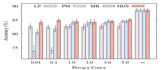
(a) Cora

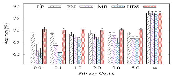
(b) Citeseer

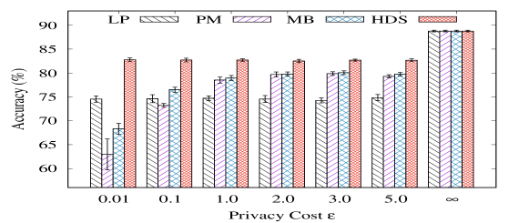
(c) Pubmed

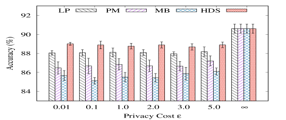
(d) LastFM

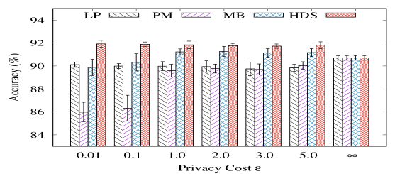
(e) Facebook

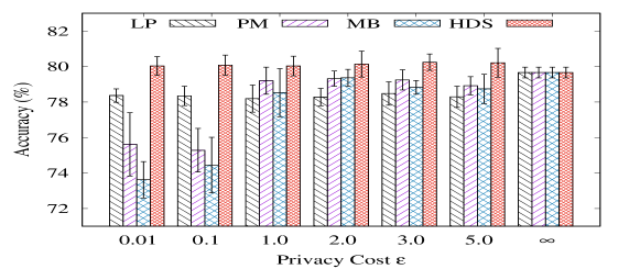
(f) Wikipedia

Figure 2: Trade-offs between privacy and accuracy under different LDP mechanisms in node classification. Note that the error bars represent the standard deviation and the results for $\infty$ denote the accuracy of the non-private baselines.

Node Classification. In the first set of experiments, we assess the accuracy performance of various perturbed mechanisms under different privacy budgets for node classification. The privacy budget is varied within $\{0.01,0.1,1.0,2.0,3.0,5.0,\infty\}$ and we report the accuracy of each method under each privacy budget, as depicted in Figure 2. Note that the error bars in the Figure 2 represent the standard deviation. In addition, the case where $\epsilon=\infty$ is provided for comparison with non-private baselines, where node features are directly employed without any perturbation.

According to the experimental results, we make the following observations. First, our proposed method demonstrates robustness to the perturbations and achieves comparable performance to the non-private baseline across all datasets. For instance, on the LastFM dataset, the HDS mechanism achieves an accuracy of about 89.0% at $\epsilon=0.01$, with only a 1.6% decrease compared to the non-private method ($\epsilon=\infty$). On the Cora dataset, the HDS mechanism’s accuracy at $\epsilon=0.01$ is approximately 84.2%, just 4.3% lower than the non-private method. Similarly, our approach incurs less than 7.0% accuracy loss compared to the non-private baseline when $\epsilon=0.01$ on both the Citeseer and Pubmed datasets. Interestingly, on the Facebook and Wikipedia datasets, our perturbation algorithm’s accuracy is roughly 1.2 and 0.4 percentage points higher than the non-private setting, respectively. We conjecture that the observed experimental results are mainly due to the injecting noise providing the model with strong generalization ability. Furthermore, our algorithm’s performance remains stable under each privacy budget setting, with only minimal standard deviation values. It consistently exhibits similar accuracy across highly distinct privacy budget values, ranging from $0.01$ to $1.0$, which serves as compelling evidence of its robustness to perturbations.

Second, our HDS mechanism consistently outperforms the other methods in almost all cases, particularly under smaller privacy budgets, which aligns with the theoretical analysis in Theorem 2. For instance, at $\epsilon=0.01$, HDS achieves approximately 8.2% higher accuracy than the best competitor, the Laplace mechanism, on the Pubmed dataset. Similarly, at $\epsilon=0.01$, our approach outperforms LP, PM, and MB by 2.0%, 8.5% and 9.8%, respectively, on the Citeseer dataset. This significant performance advantage can be attributed to the fact that our proposed perturbation mechanism can provide more concentrated perturbations compared to the Laplace, Piecewise, and Multi-bit mechanisms. Additionally, we can observe that even the most straightforward method, the Laplace mechanism, can sometimes outperform the Piecewise and Multi-bit mechanisms in the node classification task, especially when a smaller privacy budget is assigned.

TABLE III: Trade-offs between privacy and AUC under different LDP mechanisms in link prediction. Note that the results for $\infty$ denote the AUC of the non-private baselines.

Dataset	Mech.	$\epsilon=1.0$	$\epsilon=2.0$	$\epsilon=3.0$	$\epsilon=5.0$	$\epsilon=\infty$
Cora	LP	$75.22\pm 3.12$	$76.00\pm 3.48$	$74.95\pm 3.71$	$75.20\pm 3.63$	$93.07\pm 0.25$
	PM	$73.20\pm 3.16$	$78.17\pm 1.08$	$77.78\pm 1.67$	$75.20\pm 2.12$	$93.07\pm 0.25$
	MB	$75.92\pm 1.78$	$78.46\pm 1.41$	$78.52\pm 1.09$	$76.61\pm 0.86$	$93.07\pm 0.25$
	HDS	$\bm{82.43}\pm\bm{1.47}$	$\bm{82.66}\pm\bm{0.83}$	$\bm{82.50}\pm\bm{0.94}$	$\bm{82.25}\pm\bm{0.77}$	$93.07\pm 0.25$
Citeseer	LP	$71.59\pm 3.31$	$70.19\pm 3.32$	$70.82\pm 2.23$	$68.27\pm 3.77$	$94.95\pm 0.48$
	PM	$76.51\pm 1.10$	$76.28\pm 0.65$	$76.13\pm 0.57$	$74.48\pm 1.29$	$94.95\pm 0.48$
	MB	$75.27\pm 1.29$	$73.86\pm 1.65$	$74.72\pm 1.40$	$75.22\pm 0.79$	$94.95\pm 0.48$
	HDS	$\bm{77.65}\pm\bm{0.38}$	$\bm{77.64}\pm\bm{0.46}$	$\bm{77.28}\pm\bm{0.46}$	$\bm{77.71}\pm\bm{0.24}$	$94.95\pm 0.48$
Pubmed	LP	$62.84\pm 0.61$	$63.24\pm 1.15$	$64.34\pm 0.78$	$64.42\pm 0.53$	$97.46\pm 0.02$
	PM	$79.04\pm 1.03$	$77.03\pm 1.24$	$76.74\pm 1.49$	$74.93\pm 0.46$	$97.46\pm 0.02$
	MB	$79.35\pm 0.80$	$77.85\pm 1.04$	$78.39\pm 0.69$	$77.24\pm 0.66$	$97.46\pm 0.02$
	HDS	$\bm{79.50}\pm\bm{1.50}$	$\bm{79.64}\pm\bm{1.61}$	$\bm{80.11}\pm\bm{0.23}$	$\bm{79.60}\pm\bm{1.46}$	$97.46\pm 0.02$
Lastfm	LP	$74.41\pm 6.32$	$75.41\pm 5.95$	$77.01\pm 4.84$	$73.77\pm 3.45$	$95.93\pm 0.09$
	PM	$67.90\pm 0.91$	$71.70\pm 6.22$	$71.96\pm 3.92$	$80.07\pm 1.42$	$95.93\pm 0.09$
	MB	$75.69\pm 3.09$	$78.18\pm 3.25$	$78.89\pm 4.60$	$77.96\pm 3.27$	$95.93\pm 0.09$
	HDS	$\bm{91.73}\pm\bm{1.30}$	$\bm{92.03}\pm\bm{0.08}$	$\bm{92.01}\pm\bm{0.08}$	$\bm{91.98}\pm\bm{0.11}$	$95.93\pm 0.09$
Facebook	LP	$81.92\pm 3.20$	$84.66\pm 2.67$	$85.63\pm 1.05$	$86.00\pm 1.17$	$95.60\pm 0.07$
	PM	$92.05\pm 0.52$	$93.20\pm 0.54$	$93.25\pm 0.33$	$89.86\pm 0.30$	$95.60\pm 0.07$
	MB	$92.62\pm 3.75$	$92.80\pm 2.29$	$93.10\pm 2.22$	$87.70\pm 0.94$	$95.60\pm 0.07$
	HDS	$\bm{96.70}\pm\bm{0.05}$	$\bm{96.65}\pm\bm{0.05}$	$\bm{96.64}\pm\bm{0.06}$	$\bm{96.58}\pm\bm{0.04}$	$95.60\pm 0.07$
Wikipedia	LP	$72.16\pm 2.83$	$74.78\pm 4.71$	$76.11\pm 2.46$	$75.69\pm 3.50$	$98.49\pm 0.04$
	PM	$76.94\pm 5.25$	$76.55\pm 4.57$	$76.77\pm 3.54$	$77.86\pm 1.72$	$98.49\pm 0.04$
	MB	$76.62\pm 3.61$	$77.20\pm 1.40$	$78.20\pm 1.25$	$78.37\pm 1.14$	$98.49\pm 0.04$
	HDS	$\bm{99.12}\pm\bm{0.04}$	$\bm{99.14}\pm\bm{0.05}$	$\bm{99.09}\pm\bm{0.06}$	$\bm{99.11}\pm\bm{0.05}$	$98.49\pm 0.04$

Link Prediction. In the second set of experiments, we shift our focus to another interesting task: link prediction, which aims to predict unobserved links in the graph based on the perturbed features. To investigate how LDP-GE performs under varying privacy budgets, we change $\epsilon$ from $1.0$ to $5.0$. The performance of our approach is compared with other competitors on the six datasets, and the results are summarized in Table III.

Similar to the node classification task, our HDS algorithm outperforms the other three methods in terms of the AUC score. At $\epsilon=1.0$, our proposed algorithm’s AUC score is roughly 6.5, 16.0, and 4.0 points higher than the best competitor over Cora, LastFM, and Facebook, respectively. In addition, the experimental results demonstrate that even when considering strong privacy guarantees, such as $\epsilon=1.0$, the technique still achieves acceptable AUC scores on all six datasets, especially on the LastFM, Facebook and Wikipedia datasets, where the AUC scores are above $90\%$. These outcomes underline the effectiveness of the proposed method for the link prediction task. Similar to the node classification task, our perturbation mechanism yields higher AUC scores than the non-private baseline on both Facebook and Wikipedia datasets, further confirming the high effectiveness of the proposed solution. Unlike the observations obtained from the node classification, in the link prediction task, we notice that the Laplace mechanism underperforms the Piecewise and Multi-bit mechanisms in most cases. In addition, due to the significant amount of injected noise, the performance of the three competitors becomes highly unstable, resulting in large standard deviations. Consequently, in some cases, a smaller privacy budget outperforms a larger one. In summary, the experimental results highlight the effectiveness of our approach in preserving privacy while achieving competitive performance.

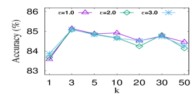
(a) Cora

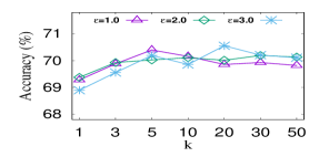
(b) Citeseer

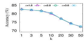
(c) Pubmed

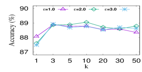
(d) LastFM

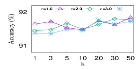
(e) Facebook

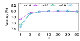
(f) Wikipedia

Figure 3: Effect of the sampling parameter $k$ on the performance of LDP-GE for node classification.

Parameter Analysis. In this experiment, we investigate the impact of the sampling parameter $k$ on our proposed method’s performance. The parameter $k$ is a hyperparameter that controls the size of the subset of dimensions that are randomly perturbed in the HDS mechanism. We change $k$ within the range $\{1,3,5,10,20,30,50\}$, and evaluate the results under different privacy budgets $\epsilon\in\{1.0,2.0,3.0\}$ for both node classification and link prediction tasks.

Regarding node classification, the experiment results are illustrated in Figure 3. We observe that the performance of our algorithm remains relatively stable across all values of $k$ in this range on Cora, Citeseer, LastFM, and Facebook datasets, varying up and down by no more than 2.0%. However, on the Pubmed dataset, the approach performs better when the value of $k$ is smaller, specifically when $k\leq 5$. Conversely, on the Wikipedia dataset, our algorithm’s performance improves with larger sampling, particularly when $k\geq 10$. This suggests that the algorithm’s performance is sensitive to the value of $k$ on the Pubmed and Wikipedia datasets, whereas it is relatively insensitive to $k$ on the other four datasets.

As for link prediction, the experiment results are illustrated in Figure 4. Our framework performs better for small values of $k$ on Cora, Citeseer, LastFM, and Facebook datasets, while it achieves better results for large $k$ values on the Pubmed dataset. On the Wikipedia dataset, our method is stable across all values of $k$ in this range. Generally, the optimal value of $k$ depends on the specific dataset and task.

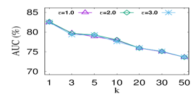
(a) Cora

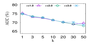
(b) Citeseer

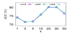
(c) Pubmed

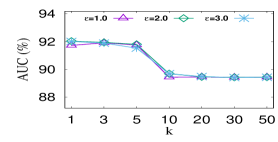
(d) LastFM

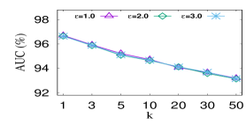
(e) Facebook

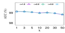
(f) Wikipedia

Figure 4: Effect of the sampling parameter $k$ on the performance of LDP-GE for link prediction.

V Related work

In this section, we review the related literature from two perspectives: graph analysis and graph learning under DP requirements.

DP on Graph Analysis. DP has emerged as the de facto standard for privacy guarantees in various data analysis tasks [18, 46]. In the centralized DP setting, most research works in graph analysis revolves around computing diverse statistics, such as degree distributions, subgraph counting, and the cost of the minimum spanning tree [47, 48, 49, 50, 51, 52]. Moreover, researchers have proposed algorithms for addressing other graph-related problems under DP constraints. For instance, some papers explore releasing subsets of nodes in the input graph while preserving DP, tackling problems like the vertex cover [53] and the densest subgraph [54, 55]. Another direction of work is to generate synthetic graphs under differential privacy [56, 57]. However, all these centralized DP algorithms require that the data collector has the personal data of all users (i.e., the entire graph), which suffer from the data breach issue.

In contrast, LDP [18] assumes an untrusted data collector. Under LDP, each user obfuscates their personal data locally and sends the obfuscated data to a (possibly malicious) data collector. Recently, LDP has gained significant attention in graph analysis. In this setting, Ye et al. [58] propose an algorithm for estimating graph metrics, including the clustering coefficient and modularity. Qin et al. [59] develop a multi-phase approach to generate synthetic decentralized social graphs under the notion of LDP.

In addition, a line of research has emerged for subgraph counting under local differential privacy [60, 15, 16]. More specifically, Sun et al. [60] design a multi-phase framework under decentralized differential privacy, which assumes that each user allows her friends to see all her connections. For triangle counts, Imola et al. [15] introduce an additional round of interaction between users and the data collector to reduce the estimation error, and [16] employs edge sampling to improve the communication efficiency. These studies demonstrate the growing interest in leveraging local differential privacy for privacy-preserving graph analysis.

DP on Graph Learning. Graph learning has become a focal point of research due to its wide applications in the real world [61]. However, applying graph learning techniques to sensitive data raises serious privacy concerns. To address these issues, one important direction is to leverage DP to protect privacy.

Several efforts have been made to incorporate DP into graph learning algorithms. Xu et al. [9] propose a DP algorithm for graph embedding, utilizing the objective perturbation mechanism [62] on the loss function of matrix factorization. Zhang et al. [10] design a perturbed gradient descent method based on the Lipschitz condition [63] for graph embedding under centralized DP. Epasto et al. [11] develop an approximate method for computing personalized PageRank vectors with differential privacy and extend this algorithm to graph embedding. Some graph learning methods, such as Graph Convolutional Network [29] and GraphSAGE [64], are based on or generalized from deep learning techniques. In recent years, DP has also been used to provide formal privacy assurances for Graph Neural Networks [12, 13, 14]. All these graph learning methods assume that there is a trusted data curator, making them susceptible to data leakage issues and unsuitable for decentralized graph analysis applications [17].

To tackle these issues, some studies have focused on leveraging LDP to train Graph Neural Networks [24, 65, 26, 25, 66]. To be specific, Zhang et al. [65] propose an algorithm for recommendation systems, which utilizes LDP to prevent users from attribute inference attacks. Nevertheless, their approach assumes a bipartite graph structure and cannot handle homogeneous graphs. LPGNN [24] assumes that node features are private and the data curator has access to the graph structure (i.e., edges in the graph), where the scenario is similar to ours. In this setting, each user perturbs their features through the Multi-bit mechanism. However, this mechanism introduces much noise to the data that can degrade the performance. Analogously, [26, 25] also utilize the Multi-bit mechanism to preserve the privacy of node features. Unlike these works, we propose an improved mechanism to achieve LDP for graph embedding and provide a detailed utility analysis for our method.

VI Conclusion

In this paper, we propose the LDP-GE framework, a privacy-preserving graph embedding framework with provable privacy guarantees based on local differential privacy. To this end, we propose an LDP mechanism, named the HDS mechanism, to protect the privacy of node features. Then, to avoid neighborhood explosion and over-smoothing issues, we decouple the feature transformation from the graph propagation and adopt personalized PageRank as the proximity measure to learn node representations. Importantly, we perform a novel theoretical analysis of the privacy and utility of the LDP-GE framework. Extensive experiments conducted over real-world datasets demonstrate that our proposed method establishes state-of-the-art performance and achieves decent privacy-utility trade-offs on both node classification and link prediction tasks. For future work, we plan to extend our work to protect the privacy of graph structure as well. Another promising future direction is to develop a graph embedding algorithm to preserve the edge privacy of non-attributed graphs that contain only node IDs and edges.

References

- [1] J. Qiu, J. Tang, H. Ma, Y. Dong, K. Wang, and J. Tang, “Deepinf: Social influence prediction with deep learning,” in Proceedings of the 24th ACM SIGKDD international conference on knowledge discovery and data mining, 2018, pp. 2110–2119.
- [2] J. Wang, S. Zhang, Y. Xiao, and R. Song, “A review on graph neural network methods in financial applications,” arXiv preprint arXiv:2111.15367, 2021.
- [3] Z. Diao, X. Wang, D. Zhang, Y. Liu, K. Xie, and S. He, “Dynamic spatial-temporal graph convolutional neural networks for traffic forecasting,” in Proceedings of the 33rd AAAI conference on artificial intelligence, 2019, pp. 890–897.
- [4] Y. Yin and Z. Wei, “Scalable graph embeddings via sparse transpose proximities,” in Proceedings of the 25th ACM SIGKDD International Conference on Knowledge Discovery and Data Mining, 2019, pp. 1429–1437.
- [5] J. Qiu, Y. Dong, H. Ma, J. Li, C. Wang, K. Wang, and J. Tang, “Netsmf: Large-scale network embedding as sparse matrix factorization,” in The World Wide Web Conference, 2019, pp. 1509–1520.
- [6] X. Zhang, K. Xie, S. Wang, and Z. Huang, “Learning based proximity matrix factorization for node embedding,” in Proceedings of the 27th ACM SIGKDD Conference on Knowledge Discovery and Data Mining, 2021, pp. 2243–2253.
- [7] H. Wang, M. He, Z. Wei, S. Wang, Y. Yuan, X. Du, and J.-R. Wen, “Approximate graph propagation,” in Proceedings of the 27th ACM SIGKDD Conference on Knowledge Discovery and Data Mining, 2021, pp. 1686–1696.
- [8] C. Dwork, F. McSherry, K. Nissim, and A. Smith, “Calibrating noise to sensitivity in private data analysis,” in Theory of cryptography conference, 2006, pp. 265–284.
- [9] D. Xu, S. Yuan, X. Wu, and H. Phan, “Dpne: Differentially private network embedding,” in Pacific-Asia Conference on Knowledge Discovery and Data Mining, 2018, pp. 235–246.
- [10] S. Zhang and W. Ni, “Graph embedding matrix sharing with differential privacy,” IEEE Access, vol. 7, pp. 89 390–89 399, 2019.
- [11] A. Epasto, V. Mirrokni, B. Perozzi, A. Tsitsulin, and P. Zhong, “Differentially private graph learning via sensitivity-bounded personalized pagerank,” arXiv preprint arXiv:2207.06944, 2022.
- [12] A. Daigavane, G. Madan, A. Sinha, A. G. Thakurta, G. Aggarwal, and P. Jain, “Node-level differentially private graph neural networks,” arXiv preprint arXiv:2111.15521, 2021.
- [13] A. Kolluri, T. Baluta, B. Hooi, and P. Saxena, “Lpgnet: Link private graph networks for node classification,” in Proceedings of the 2022 ACM SIGSAC Conference on Computer and Communications Security, 2022, pp. 1813–1827.
- [14] S. Sajadmanesh, A. S. Shamsabadi, A. Bellet, and D. Gatica-Perez, “Gap: Differentially private graph neural networks with aggregation perturbation,” arXiv preprint arXiv:2203.00949, 2022.
- [15] J. Imola, T. Murakami, and K. Chaudhuri, “Locally differentially private analysis of graph statistics,” in 30th USENIX Security Symposium, 2021, pp. 983–1000.
- [16] J. Imola, T. Murakami, and K. Chaudhuri, “Communication-efficient triangle counting under local differential privacy,” in 31st USENIX Security Symposium, 2022, pp. 537–554.
- [17] T. Paul, A. Famulari, and T. Strufe, “A survey on decentralized online social networks,” Computer Networks, vol. 75, pp. 437–452, 2014.
- [18] S. P. Kasiviswanathan, H. K. Lee, K. Nissim, S. Raskhodnikova, and A. Smith, “What can we learn privately?” SIAM Journal on Computing, vol. 40, no. 3, pp. 793–826, 2011.
- [19] Ú. Erlingsson, V. Pihur, and A. Korolova, “Rappor: Randomized aggregatable privacy-preserving ordinal response,” in Proceedings of the 2014 ACM SIGSAC conference on computer and communications security, 2014, pp. 1054–1067.
- [20] J. Tang, A. Korolova, X. Bai, X. Wang, and X. Wang, “Privacy loss in apple’s implementation of differential privacy on macos 10.12,” arXiv preprint arXiv:1709.02753, 2017.
- [21] B. Ding, J. Kulkarni, and S. Yekhanin, “Collecting telemetry data privately,” in Advances in Neural Information Processing Systems 30, 2017, pp. 3571–3580.
- [22] J. C. Duchi, M. I. Jordan, and M. J. Wainwright, “Minimax optimal procedures for locally private estimation,” Journal of the American Statistical Association, vol. 113, no. 521, pp. 182–201, 2018.
- [23] N. Wang, X. Xiao, Y. Yang, J. Zhao, S. C. Hui, H. Shin, J. Shin, and G. Yu, “Collecting and analyzing multidimensional data with local differential privacy,” in 2019 IEEE 35th International Conference on Data Engineering (ICDE), 2019, pp. 638–649.
- [24] S. Sajadmanesh and D. Gatica-Perez, “Locally private graph neural networks,” in Proceedings of the 2021 ACM SIGSAC Conference on Computer and Communications Security, 2021, pp. 2130–2145.
- [25] H. Jin and X. Chen, “Gromov-wasserstein discrepancy with local differential privacy for distributed structural graphs,” in Proceedings of the 31st International Joint Conference on Artificial Intelligence, 2022, pp. 2115–2121.
- [26] W. Lin, B. Li, and C. Wang, “Towards private learning on decentralized graphs with local differential privacy,” IEEE Transactions on Information Forensics and Security, vol. 17, pp. 2936–2946, 2022.
- [27] C. Dwork, “Differential privacy: A survey of results,” in International conference on theory and applications of models of computation, 2008, pp. 1–19.
- [28] J. Gilmer, S. S. Schoenholz, P. F. Riley, O. Vinyals, and G. E. Dahl, “Neural message passing for quantum chemistry,” in Proceedings of the 34th International Conference on Machine Learning, 2017, pp. 1263–1272.
- [29] T. N. Kipf and M. Welling, “Semi-supervised classification with graph convolutional networks,” in Proceedings of the 5th International Conference on Learning Representations, 2017.
- [30] P. Veličković, G. Cucurull, A. Casanova, A. Romero, P. Lio, and Y. Bengio, “Graph attention networks,” arXiv preprint arXiv:1710.10903, 2017.
- [31] M. Liu, H. Gao, and S. Ji, “Towards deeper graph neural networks,” in Proceedings of the 26th ACM SIGKDD international conference on knowledge discovery and data mining, 2020, pp. 338–348.
- [32] A. Bojchevski, J. Klicpera, B. Perozzi, A. Kapoor, M. Blais, B. Rózemberczki, M. Lukasik, and S. Günnemann, “Scaling graph neural networks with approximate pagerank,” in Proceedings of the 26th ACM SIGKDD International Conference on Knowledge Discovery and Data Mining, 2020, pp. 2464–2473.
- [33] J. Klicpera, A. Bojchevski, and S. Günnemann, “Predict then propagate: Graph neural networks meet personalized pagerank,” in Proceedings of the 7th International Conference on Learning Representations, 2019.
- [34] J. Klicpera, S. Weißenberger, and S. Günnemann, “Diffusion improves graph learning,” in Advances in Neural Information Processing Systems 32, 2019, pp. 13 333–13 345.
- [35] F. Wu, A. Souza, T. Zhang, C. Fifty, T. Yu, and K. Weinberger, “Simplifying graph convolutional networks,” in Proceedings of the 36th International Conference on Machine Learning, 2019, pp. 6861–6871.
- [36] M. Chen, Z. Wei, B. Ding, Y. Li, Y. Yuan, X. Du, and J.-R. Wen, “Scalable graph neural networks via bidirectional propagation,” in Advances in Neural Information Processing Systems 33, 2020, pp. 14 556–14 566.
- [37] L. Page, S. Brin, R. Motwani, and T. Winograd, “The pagerank citation ranking: bringing order to the web,” Stanford InfoLab, Tech. Rep., 1999.
- [38] Z. Li, T. Wang, M. Lopuhaä-Zwakenberg, N. Li, and B. Škoric, “Estimating numerical distributions under local differential privacy,” in Proceedings of the 2020 ACM SIGMOD International Conference on Management of Data, 2020, pp. 621–635.
- [39] J. Duan, Q. Ye, and H. Hu, “Utility analysis and enhancement of ldp mechanisms in high-dimensional space,” in 2022 IEEE 38th International Conference on Data Engineering (ICDE), 2022, pp. 407–419.
- [40] B. Rozemberczki and R. Sarkar, “Characteristic functions on graphs: Birds of a feather, from statistical descriptors to parametric models,” in Proceedings of the 29th ACM international conference on information and knowledge management, 2020, pp. 1325–1334.
- [41] B. Rozemberczki, C. Allen, and R. Sarkar, “Multi-scale attributed node embedding,” Journal of Complex Networks, vol. 9, no. 2, p. cnab014, 2021.
- [42] Z. Wang, Y. Zhou, L. Hong, Y. Zou, and H. Su, “Pairwise learning for neural link prediction,” arXiv preprint arXiv:2112.02936, 2021.
- [43] J. Lv, Z. Li, H. Chen, Y. Qi, and C. Wu, “Path-aware siamese graph neural network for link prediction,” arXiv preprint arXiv:2208.05781, 2022.
- [44] Microsoft, “Neural Network Intelligence,” 1 2021. [Online]. Available: https://github.com/microsoft/nni
- [45] D. P. Kingma and J. Ba, “Adam: A method for stochastic optimization,” in Proceedings of the 3rd International Conference on Learning Representations, 2015.
- [46] J. C. Duchi, M. I. Jordan, and M. J. Wainwright, “Local privacy and statistical minimax rates,” in 2013 IEEE 54th Annual Symposium on Foundations of Computer Science, 2013, pp. 429–438.
- [47] K. Nissim, S. Raskhodnikova, and A. Smith, “Smooth sensitivity and sampling in private data analysis,” in Proceedings of the 39th Annual ACM symposium on Theory of computing, 2007, pp. 75–84.
- [48] V. Karwa, S. Raskhodnikova, A. Smith, and G. Yaroslavtsev, “Private analysis of graph structure,” Proceedings of the VLDB Endowment, vol. 4, no. 11, pp. 1146–1157, 2011.
- [49] S. P. Kasiviswanathan, K. Nissim, S. Raskhodnikova, and A. Smith, “Analyzing graphs with node differential privacy,” in Theory of Cryptography Conference, 2013, pp. 457–476.
- [50] J. Zhang, G. Cormode, C. M. Procopiuc, D. Srivastava, and X. Xiao, “Private release of graph statistics using ladder functions,” in Proceedings of the 2015 ACM SIGMOD international conference on management of data, 2015, pp. 731–745.
- [51] W.-Y. Day, N. Li, and M. Lyu, “Publishing graph degree distribution with node differential privacy,” in Proceedings of the 2016 International Conference on Management of Data, 2016, pp. 123–138.
- [52] X. Ding, S. Sheng, H. Zhou, X. Zhang, Z. Bao, P. Zhou, and H. Jin, “Differentially private triangle counting in large graphs,” IEEE Transactions on Knowledge and Data Engineering, 2021.
- [53] A. Gupta, K. Ligett, F. McSherry, A. Roth, and K. Talwar, “Differentially private combinatorial optimization,” in Proceedings of the 21st Annual ACM-SIAM Symposium on Discrete Algorithms, 2010, pp. 1106–1125.
- [54] D. Nguyen and A. Vullikanti, “Differentially private densest subgraph detection,” in Proceedings of the 38th International Conference on Machine Learning, 2021, pp. 8140–8151.
- [55] L. Dhulipala, Q. C. Liu, S. Raskhodnikova, J. Shi, J. Shun, and S. Yu, “Differential privacy from locally adjustable graph algorithms: k-core decomposition, low out-degree ordering, and densest subgraphs,” in 2022 IEEE 63rd Annual Symposium on Foundations of Computer Science (FOCS), 2022, pp. 754–765.
- [56] Q. Xiao, R. Chen, and K.-L. Tan, “Differentially private network data release via structural inference,” in Proceedings of the 20th ACM SIGKDD international conference on Knowledge discovery and data mining, 2014, pp. 911–920.
- [57] Z. Jorgensen, T. Yu, and G. Cormode, “Publishing attributed social graphs with formal privacy guarantees,” in Proceedings of the 2016 international conference on management of data, 2016, pp. 107–122.
- [58] Q. Ye, H. Hu, M. H. Au, X. Meng, and X. Xiao, “Towards locally differentially private generic graph metric estimation,” in 2020 IEEE 36th International Conference on Data Engineering (ICDE), 2020, pp. 1922–1925.
- [59] Z. Qin, T. Yu, Y. Yang, I. Khalil, X. Xiao, and K. Ren, “Generating synthetic decentralized social graphs with local differential privacy,” in Proceedings of the 2017 ACM SIGSAC Conference on Computer and Communications Security, 2017, pp. 425–438.
- [60] H. Sun, X. Xiao, I. Khalil, Y. Yang, Z. Qin, H. Wang, and T. Yu, “Analyzing subgraph statistics from extended local views with decentralized differential privacy,” in Proceedings of the 2019 ACM SIGSAC Conference on Computer and Communications Security, 2019, pp. 703–717.
- [61] F. Xia, K. Sun, S. Yu, A. Aziz, L. Wan, S. Pan, and H. Liu, “Graph learning: A survey,” IEEE Transactions on Artificial Intelligence, vol. 2, no. 2, pp. 109–127, 2021.
- [62] K. Chaudhuri, C. Monteleoni, and A. D. Sarwate, “Differentially private empirical risk minimization,” Journal of Machine Learning Research, vol. 12, no. 3, 2011.
- [63] M. Jha and S. Raskhodnikova, “Testing and reconstruction of lipschitz functions with applications to data privacy,” SIAM Journal on Computing, vol. 42, no. 2, pp. 700–731, 2013.
- [64] W. Hamilton, Z. Ying, and J. Leskovec, “Inductive representation learning on large graphs,” in Advances in Neural Information Processing Systems 30, 2017, pp. 1024–1034.
- [65] S. Zhang, H. Yin, T. Chen, Z. Huang, L. Cui, and X. Zhang, “Graph embedding for recommendation against attribute inference attacks,” in Proceedings of the Web Conference 2021, 2021, pp. 3002–3014.
- [66] S. Hidano and T. Murakami, “Degree-preserving randomized response for graph neural networks under local differential privacy,” arXiv preprint arXiv:2202.10209, 2022.