Robust Trading in a Generalized Lattice Market

Abstract

This paper introduces a novel robust trading paradigm, called multi-double linear policies, situated within a generalized lattice market. Distinctively, our framework departs from most existing robust trading strategies, which are predominantly limited to single or paired assets and typically embed asset correlation within the trading strategy itself, rather than as an inherent characteristic of the market. Our generalized lattice market model incorporates both serially correlated returns and asset correlation through a conditional probabilistic model. In the nominal case, where the parameters of the model are known, we demonstrate that the proposed policies ensure survivability and probabilistic positivity. We then derive an analytic expression for the worst-case expected gain-loss and prove sufficient conditions that the proposed policies can maintain a positive expected profits, even within a seemingly nonprofitable symmetric lattice market. When the parameters are unknown and require estimation, we show that the parameter space of the lattice model forms a convex polyhedron, and we present an efficient estimation method using a constrained least-squares method. These theoretical findings are strengthened by extensive empirical studies using data from the top 30 companies within the S&P 500 index, substantiating the efficacy of the generalized model and the robustness of the proposed policies in sustaining the positive expected profit and providing downside risk protection.

1 Introduction

The robustness of algorithmic trading systems has been a focal point of numerous studies such as dokuchaev1998asymptotic, dokuchaev2002dynamic, korajczyk2004momentum, barmish2008trading. Among the various aspects of robustness, the Robust Positive Expectation (RPE), a trading policy capable of generating a positive expected profit across various market conditions, is particularly sought after. Notably, among the strategies targeting RPE, the so-called Simultaneous Long-Short (SLS) strategy, proposed by barmish2011arbitrage, barmish2015new, has proven to be a significant advancement. This strategy involves investors holding both long and short positions simultaneously, with equal weights, that leverages market movements in either direction.

Subsequently, several extensions have been proposed to the SLS strategy, including generalization for Merton’s diffusion model in baumann2016stock, geometric Brownian motion (GBM) model with time-varying parameters in primbs2017robustness, and any linear stochastic differential equation (SDE) in baumann2019positive. Additionally, the SLS strategy has also been extended to the proportional-integral (PI) controller in malekpour2018generalization, to latency trading in malekpour2016stock, and coupled SLS strategy on pair trading for two correlated assets was studied in deshpande2018generalization, deshpande2020simultaneous. Recent contributions to the SLS theory include the work by baumann2023theoretical.

Other innovative approaches have focused on robust stock trading. For example, maroni2019robust proposed a robust design strategy for stock trading via feedback control. primbs2018pairs, tie2018optimal studied the stochastic control-theoretic approach in a pair trading framework, vitale2018robust investigated robust trading for ambiguity-averse insider, o2020generalized proposed a generalized SLS with different weight settings on long and short positions. Recently, hsieh2022robust introduced a new variant of the SLS strategy, termed the double linear policy, which assigns equal weights to long and short positions in a discrete-time setting, creating a mean-variance criterion to determine optimal weights. This work was later extended by wang2023robustness to involve time-varying weights, under the assumption of serially independent returns.

Despite numerous contributions to the robust trading systems, a crucial gap persists in the existing literature. Most existing strategies, including SLS or double linear policy, are limited to single or paired assets, and often model asset correlation within the trading strategy, rather than considering it as a characteristic of the market. More importantly, they often overlook serial dependence in asset returns, a notable empirical phenomenon fielitz1971stationarity, officer1972distribution, campbell1993trading, christoffersen2006financial. While the work by balvers1997autocorrelated investigated autocorrelated returns and optimal intertemporal portfolio choice, it primarily focuses on short-term memory, and more importantly, it does not address the robustness of the strategy in various market conditions. These omissions pose a significant challenge in robust trading strategies, as emphasized by recent work that highlights the impact of tick-size reductions on various stocks and the influence of competing crossing networks werner2023tick.

In response to these gaps, this paper introduces an extension to the double linear policy, termed multi-double linear policies. We rigorously investigate its stochastic robustness in a generalized lattice market that involves both serial and asset correlations, as detailed in Section 2. Then we demonstrate that the proposed policies ensure survivability and probabilistic positivity. Following this, we establish a detailed gain-loss analysis and derive an analytic expression of the worst-case expected gain-loss function. We then prove that the proposed policies offer a form of downside risk protection in comparison to the pure long-only and pure short-only strategies. We demonstrate an “approximate” RPE in Section 3 and establish sufficient conditions under which the positive expected profit is upheld, even within a symmetric lattice market, thereby underscoring the theoretical foundations of our approach. We further show that the parameters used in the proposed generalized lattice model form a convex polyhedron, which facilitates efficient estimation through a constrained least-squares approach; see Section 4. These theoretical findings are substantiated by extensive empirical studies, lending practical relevance to the developed framework; see Section 5.

2 Preliminaries and Notations

This section provides an overview of the formulation, including the generalized lattice market with binomial serially correlated returns and asset correlation, the multi-double linear policies, and the robust positive expectation property.

2.1 Generalized Lattice Market with Serial and Asset Correlations

Consider a lattice market consisting of $n\geq 1$ distinct assets. For each asset, say Asset $i$ with $i\in\{1,2,\dots,n\}$, the per-period returns are represented by the sequence $\{X_{i}(k):k\geq 0\}$. These returns exhibit two possible outcomes, with $X_{i}(k)\in\{u_{i},d_{i}\}$, where $u_{i}\in(0,1)$ represents the upward movement factor and $d_{i}\in(-1,0)$ represents the downward movement factor. In combination, this holds for all stages $k$ satisfying $-1<d_{i}<0<u_{i}<1$ for $i=1,2,\dots,n$. The generalization of the model stems from the assumption that there are asset correlations and serial correlations in the probability of returns, signifying that a positive return at each stage depends on the previous stages and other assets.

In particular, we assume that the return process $\{X_{i}(k):k\geq 0\}$ with $X_{i}(k)\in\{u_{i},d_{i}\}$, exhibits Markov memory with serial autocorrelation and asset correlation. Specifically, take the vector of returns at stage $k$ as $X(k):=[X_{1}(k)\;X_{2}(k)\cdots X_{n}(k)]^{\top}$, the vector of upward movement factors as $U:=[u_{1}\;u_{2}\;\cdots\;u_{n}]^{\top}$, and the vector of downward movement factors as $D:=[d_{1}\;d_{2}\;\cdots d_{n}]^{\top}$. Henceforth, we use the shorthand $X(k-1:k-m):=(X(k-1),X(k-2),\dots,X(k-m))$. Denote the matrix of autocorrelation coefficients as $\Phi:=[\Phi_{i,j}]\in\mathbb{R}^{n\times m+1}$ where $i=1,2,\dots,n$ and $j=0,1,2,\dots,m$ and the matrix of asset correlation coefficients as $\Gamma:=[\Gamma_{i,\ell}]\in\mathbb{R}^{n\times n}$ where $i,\ell=1,2,\dots,n$. Let $\textbf{P}^{U}(k;X(k-1:k-m))$ be the vector of conditional probabilities of positive returns at stage $k$, affected by the previous $m$ stages and asset correlations. The $i$th component of this vector is given by $[\textbf{P}^{U}(k;X(k-1:k-m))]_{i}:=\mathbb{P}\left(X_{i}(k)=u_{i}\mid X(k-1:k-m)\right)\in[0,1]$. Hence,

$$\textbf{P}^{U}(k;X(k-1:k-m)) =\Phi_{0}+\begin{bmatrix}\sum_{j=1}^{m}\Phi_{1,j}X_{1}(k-j)\\ \vdots\\ \sum_{j=1}^{m}\Phi_{n,j}X_{n}(k-j)\end{bmatrix}+\Gamma X(k-1).$$ (1)

where $\Phi_{0}$ is the first column of the matrix $\Phi=[\Phi_{0},\Phi_{1},\dots,\Phi_{m}]$. Therefore, for Asset $i$, the conditional probability

$$\mathbb{P}\left(X_{i}(k)=u_{i}\mid X(k-1:k-m)\right) =\Phi_{i,0}+\sum_{j=1}^{m}\Phi_{i,j}X_{i}(k-j)+\sum_{\ell=1}^{n}\Gamma_{i,\ell}X_{\ell}(k-1)\in[0,1],$$ (2)

where $\Phi_{i,0},\Phi_{i,1},\dots,\Phi_{i,m}$ are the elements of the $i$th row of the matrix $\Phi$ and $\Gamma_{i,\ell}$ represents the $i$th row and $\ell$th column of the matrix $\Gamma$ and the conditional probabilities include initial conditions $X_{i}(-j)=x_{i}(-j)\in\{u_{i},d_{i}\}$ for $j=1,2,\dots,m$. Figure 1 illustrates the idea of the generalized lattice model with Markov memory, specifically for $m=1$ (indicating one memory length) and $n=2$ (representing two distinct assets). The figure includes the initial realized return $(x_{1}(-1),x_{2}(-1))$ for the two assets, demonstrating the probability for Asset 1 at each stage is dependent on the realized returns from the preceding stage.

Our analysis assumes that the trades incur zero transaction costs and that the underlying asset has perfect liquidity. Fractional shares are allowed. This setting serves as an appropriate starting point for building the model and aligns closely to the standard frictionless market framework in finance; see cvitanic2004introduction, luenberger2013investment. While not analyzed in theory, later in Section 5, some of the assumptions such as transaction costs are relaxed in empirical studies.

Remark 2.1.

$(i)$ Returns often exhibit serial correlation, see fielitz1971stationarity, campbell1993trading, christoffersen2006financial, with past returns over several periods. This can be due to factors like momentum, mean reversion, or other market dynamics, allowing the model to capture long-term dependencies in the return process. $(ii)$ The correlation matrix $\Gamma$ can be extended to time-dependent correlations $\Gamma(k)=f(X(k-1:k-m))$ where $f$ is a function that captures the dependence of the correlation on past returns.

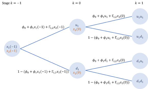
Figure 1: An Illustration of Generalized Lattice Model.

2.2 Multi-Double Linear Policies

Building upon hsieh2022robust, hsieh2022robustness, we generalize the single double linear policy, initially constructed for the single asset case, to multi-double linear policies for multi-asset portfolio case. This generalization allows for trading a portfolio consisting of $n\geq 1$ distinct assets. Beginning with an initial account value of an investor, $V(0):=V_{0}>0$, which is to be allocated across the $n$ assets using the fractions $v_{i}\in[0,1]$ for $i=1,2,\dots,n$ satisfying $\sum_{i=1}^{n}v_{i}=1$. That is, the initial account value for Asset $i$ is given by $V_{i,0}:=v_{i}V_{0}$ and the initial account $V(0)$ is a convex combination of $V_{i,0}$.

Thereafter, we strategically divide it into two parts for each asset, representing long and short positions. Superficially, take a fraction $\alpha\in[0,1]$, such that the initial account value for the long position of Asset $i$ is $V_{i,L}(0):=\alpha V_{i,0}$, and the value for the short position is $V_{i,S}(0):=(1-\alpha)V_{i,0}$. The trading policy for Asset $i$, denoted by $\pi_{i}(\cdot)$, is constructed as the sum of the policies for long and short positions, i.e., $\pi_{i}(k):=\pi_{i,L}(k)+\pi_{i,S}(k),$ where $\pi_{i,L}$ and $\pi_{i,S}$ are in double linear forms: $\pi_{i,L}(k)=w_{i}V_{i,L}(k)$ and $\pi_{i,S}(k)=-w_{i}V_{i,S}(k),$ where $w_{i}\in\mathcal{W}:=[0,1]$ is the weight for Asset $i$. Here, $V_{i,L}(k)$ and $V_{i,S}(k)$ represent the account value for the long and short positions of Asset $i$ at stage $k$, respectively. The long-short account value dynamics for Asset $i$ are given by

$$\begin{cases}V_{i,L}(k+1)=V_{i,L}(k)+\pi_{i,L}(k)X_{i}(k)+(V_{i,L}(k)-\pi_{i,L}(k))r_{f};\\ V_{i,S}(k+1)=V_{i,S}(k)+\pi_{i,S}(k)X_{i}(k),\end{cases}$$

where $r_{f}\geq 0$ is the risk-free rate. The overall account value at stage $k$ is given

$$V(k) =\sum_{i=1}^{n}(V_{i,L}(k)+V_{i,S}(k))$$

$$=\sum_{i=1}^{n}V_{i,0}\left(\alpha R_{i+}(k)+(1-\alpha)R_{i-}(k)\right),$$

where $V_{i,0}=v_{i}V_{0}$, $V_{i,L}(k)=\alpha V_{i,0}R_{i+}(k)$, and $V_{i,S}(k)=(1-\alpha)V_{i,0}R_{i-}(k)$ with $R_{i+}(k):=\prod_{j=0}^{k-1}\left((1+r_{f})+w_{i}(X_{i}(j)-r_{f})\right)$ and $R_{i-}(k):=\prod_{j=0}^{k-1}\left(1-w_{i}X_{i}(j)\right)$. Note that if $\alpha=1$, the policies correspond to a pure long-only position, while $\alpha=0$ corresponds to a pure short position. Therefore, one immediately sees that the proposed policies greatly generalize the common trading strategies.

Remark 2.2.

It should be noted that the notations $V(k)$ or $V_{i,L}(k)$ or $V_{i,S}(k)$, which implicitly depend on various parameters and variables, are suppressed for the sake of simplicity. In particular, the overall account value at stage $k$ can be expressed as $V(k)=V\left(k;(\alpha,w,v),r_{f},\{X(j)\}_{j=0}^{k-1},V_{0}\right)$ where $(\alpha,w,v)\in[0,1]\times[0,1]^{n}\times\mathcal{V}$ is the triple for the proposed polices with $\mathcal{V}:=\{v\in\mathbb{R}^{n}:v_{i}\in[0,1],\;\sum_{i=1}^{n}v_{i}=1\}$, $r_{f}\geq 0$ is the risk-free rate, and $\{X(j)\}_{j=0}^{k-1}$ denote the sequence of asset returns vectors up to stage $k-1$.

2.3 Robust Positive Expected Profits

For $k>0$, let $\mathcal{G}(k):=V(k)-V_{0}$ be the cumulative gain-loss function up to stage $k$ where $V(k)$ is the account value at stage $k$. Note that, for the sake of simplicity, we express $\mathcal{G}(k)=\mathcal{G}\left(k;(\alpha,w,v),r_{f},\{X(j)\}_{j=0}^{k-1},V_{0}\right)$. Then the expected cumulative gain-loss function is denoted by $\overline{\mathcal{G}}(k):=\mathbb{E}[\mathcal{G}(k)]$. The primary stochastic robustness to be studied in this paper is the so-called robust positive expectation (RPE) property, see the definition below.

Definition 2.1 (Robust Positive Expectation).

For stage $k=0,1,\dots$, let $V_{0}>0$ be the initial account value, and $V(k)$ be the account value at stage $k$. Define the expected cumulative gain-loss function up to stage $k$ as $\overline{\mathcal{G}}(k):=\mathbb{E}[V(k)]-V_{0}.$ A trading policy is said to have a robust positive expectation (RPE) property if it ensures that $\overline{\mathcal{G}}(k)>0$ for all $k>1$, with nonzero trend and finite variance.

2.4 Notation

We denote by $\mathbb{R}_{+}$ the nonnegative reals and $\mathbb{R}_{++}$ the strictly positive reals. For a set $A\in\mathbb{R}$, the indicator $\mathbb{1}_{A}$ is defined as $\mathbb{1}_{A}(x)=1$ if $x\in A$; otherwise $\mathbb{1}_{A}(x)=0$. For $a,b\in\mathbb{R}$ and $a<b$ and $n$ a positive integer, a set $(a,b)^{n}$ or $[a,b]^{n}$ with refers to the Cartesian product of the interval $(a,b)$ or $[a,b]$ with itself $n$-times.

3 Stochastic Robustness of the Policies

In this section, we analyze the stochastic robustness of the multi-double linear policies within the generalized lattice market with both serial and asset correlations. To facilitate our analysis, we use the vector notations $v:=[v_{1}\;v_{2}\;\cdots\;v_{n}]^{\top}\in\mathcal{V}$ where the set $\mathcal{V}:=\{v\in\mathbb{R}^{n}:v_{i}\in[0,1],\;\sum_{i=1}^{n}v_{i}=1\}$, and $w:=[w_{1}\;w_{2}\;\cdots\;w_{n}]^{\top}\in[0,1]^{n}$. With these notations, the multi-double linear policies, as described in Section 2, are characterized by the triple $(\alpha,w,v)\in[0,1]\times[0,1]^{n}\times\mathcal{V}.$ It is important to note that our analysis in this section assumes a nominal case in the sense that the generalized lattice model’s parameters $u_{i},d_{i},\Phi_{i,j},$ and $\Gamma_{i,\ell}$ are known. Subsequently, in Section 4, we provide an efficient least-square-based approach to estimate these parameters in a practical context.

3.1 Survivability and Probabilistic Positivity

The first result indicates that, for each Asset $i$, the multi-double linear policies assure survival trades; i.e., bankruptcy is avoided.

[Survivability] For multi-double linear policies with triple $(\alpha,w,v)\in[0,1]\times[0,1]^{n}\times\mathcal{V}$ for $i=1,\dots,n$, we have $V_{i,L}(k)\geq 0$, $V_{i,S}(k)\geq 0$ for all $i$ and all $k$ with probability one, and hence the overall account $V(k)\geq 0$ for all $k$ with probability one. Moreover, if $v_{i}>0$ for some $i$, $w_{i}\in(0,1)$, and $\alpha\in(0,1)$, then $V_{i,L}(k)>0$ and $V_{i,S}(k)>0$ and $V(k)>0$ for all $k$ with probability one.

Proof. See Appendix A.

With the aid of Lemma 3.1, we can prove a general result akin to the Paley-Zygmund inequality, regarding probabilistic positivity.

Lemma 3.1 (Probabilistic Positivity).

Fix $k>1$. For multi-double linear policies with triple $(\alpha,w,v)\in(0,1)\times(0,1)^{n}\times\mathcal{V}$, it follows that

$$\mathbb{P}(V(k)>\theta\mathbb{E}[V(k)])\geq\frac{(1-\theta)^{2}\mathbb{E}[V(k)]^{2}}{{\rm var}(V(k))+(1-\theta)^{2}\mathbb{E}[V(k)]^{2}},$$ (3)

for all $\theta\in[0,1]$.

Proof. See Appendix A.

3.2 Gain-Loss Analysis

For $k=0,1,\dots$, let $V(k)$ be the account value at stage $k$. Then the corresponding cumulative gain-loss function, as defined in Section 2, is given by $\mathcal{G}(k)=\sum_{i=1}^{n}V_{i,0}\left(\alpha R_{i+}(k)+(1-\alpha)R_{i-}(k)-1\right),$ and the expected cumulative gain-loss function as $\overline{\mathcal{G}}(k):=\mathbb{E}[\mathcal{G}(k)]$. Note that with this notation, we can rewrite Inequality (3) in terms of the cumulative gain-loss function. Indeed, observe that

$$\mathbb{P}(V(k)>\theta\mathbb{E}[V(k)]) =\mathbb{P}(\mathcal{G}(k)>\theta\mathbb{E}[V(k)]-V_{0})$$

$$=\mathbb{P}(\mathcal{G}(k)>\theta\mathbb{E}[V(k)]-\theta V_{0}+\theta V_{0}-V_{0})$$

$$=\mathbb{P}(\mathcal{G}(k)>\theta\overline{\mathcal{G}}(k)-(1-\theta)V_{0}).$$

Moreover, noting that $\mathbb{E}[V(k)]=\overline{\mathcal{G}}(k)+V_{0}$ and ${\rm var}(V(k))={\rm var}(\mathcal{G}(k))$, Lemma 3.1 becomes

$$\mathbb{P}(\mathcal{G}(k)>\theta\overline{\mathcal{G}}(k)-(1-\theta)V_{0})\geq\frac{(1-\theta)^{2}(\overline{\mathcal{G}}(k)+V_{0})^{2}}{{\rm var}(\mathcal{G}(k))+(1-\theta)^{2}(\overline{\mathcal{G}}(k)+V_{0})^{2}},$$

which characterizes the probability of cumulative gain-loss larger than the weighted sum of $\overline{\mathcal{G}}(\cdot)$ and $V_{0}$. Note that the variance of the cumulative gain-loss function, ${\rm var}(\mathcal{G}(k))$, is given by ${\rm var}(\mathcal{G}(k))={\rm var}\left(\sum_{i=1}^{n}V_{i,0}\left(\alpha R_{i+}(k)+(1-\alpha)R_{i-}(k)-1\right)\right).$ Although the analytic expression for this variance may be intractable within the generalized lattice market framework, it can be computed numerically; e.g., see later in Section 5. The next lemma indicates gain-loss under zero weight.

[Zero Weight Gain-Loss] Consider the multi-double linear policies with triple $(\alpha,w,v)\in[0,1]\times[0,1]^{n}\times\mathcal{V}$. If $w_{i}=0$ for all $i=1,\dots,n$, we have ${\mathcal{G}}(k)=\alpha((1+r_{f})^{k}-1)V_{0}\geq 0$ for all $k$ with probability one. Moreover, if the risk-free rate is zero, i.e., $r_{f}=0$, then the gain-loss function simplifies to $\mathcal{G}(k)=0$ for all $k$.

Proof. See Appendix A.

To prove our first main result, Theorem 3.1, the following two auxiliary lemmas are useful. The first one states that the probability of receiving a positive return can be characterized by a recursion formula, and the second one expresses a sum of expected logarithmic functions using the probability recursion.

[A Recursion Formula of Probability] For $i=1,2,\dots,n$, assume that $X_{i}(\cdot)\in\{u_{i},d_{i}\}$ are returns characterized by the generalized lattice model as described in Section 2.1. For $k\geq 1$, let $p_{i}(k):=\mathbb{P}(X_{i}(k)=u_{i})$ be the probability of receiving a positive return of Asset $i$ at stage $k$ with initial conditions $p_{i}(-j)=\frac{x_{i}(-j)-d_{i}}{u_{i}-d_{i}}$ for $j=1,2,\dots,m$ with $x_{i}(-j)\in\{u_{i},d_{i}\}$. Then $p_{i}(k)$ satisfies the following recursion

$$p_{i}(k) =\Phi_{i,0}+\sum_{j=1}^{m}\Phi_{i,j}[(u_{i}-d_{i})\cdot p_{i}({k-j})+d_{i}]+\sum_{\ell=1}^{n}\Gamma_{i,\ell}[(u_{\ell}-d_{\ell})\cdot p_{\ell}({k-1})+d_{\ell}].$$ (4)

Proof. See Appendix A.

Remark 3.1.

Note that the returns $X_{i}(\cdot)\in\{u_{i},d_{i}\}$ characterized by the generalized lattice model, follows a Bernoulli distribution with time-varying probability $p_{i}(\cdot)$, i.e., $X_{i}(\cdot)\sim Bernoulli(p_{i}(\cdot))$. Later in Section 5, the recursion formula (4) is useful to estimate the binomial probability for each stage.

Let $k\geq 1$ and consider assets $i=1,\dots,n$, each associated with a weight $w_{i}\in[0,1]$. Assume that $X_{i}(\cdot)\in\{u_{i},d_{i}\}$ are returns characterized by a generalized lattice model as described in Section 2.1. Then the following equality holds:

$$\sum_{j=0}^{k-1}\mathbb{E}[\log(1\pm w_{i}X_{i}(j))] =\mathbb{E}[H_{i}(k)]\log(1\pm w_{i}u_{i})+(k-\mathbb{E}[H_{i}(k)])\log(1\pm w_{i}d_{i}),$$ (5)

where $\mathbb{E}[H_{i}(k)]:=\sum_{j=0}^{k-1}p_{i}(j)\leq k$ is the expected number of receiving positive returns up to stage $k-1$, and $p_{i}(j)$ is stated in Lemma 3.2.

Proof. See Appendix A.

Theorem 3.1 (The Worst Expected Gain-Loss).

For $k>1$, consider the multi-double linear policies with triple $(\alpha,w,v)\in(0,1)\times(0,1)^{n}\times\mathcal{V}$, and assume that the return follows the lattice model described in Lemma 3.2. Then the expected gain-loss function $\overline{\mathcal{G}}(k)$ satisfies the following inequality:

$$\overline{\mathcal{G}}(k) >\sum_{i=1}^{n}V_{i,0}\left(\alpha(\beta_{i}(k)-1)+(1-\alpha)(\gamma_{i}(k)-1)\right),$$

where $\beta_{i}(k):=((1+r_{f})+w_{i}(u_{i}-r_{f}))^{\mathbb{E}[H_{i}(k)]}((1+r_{f})+w_{i}(d_{i}-r_{f}))^{\left(k-\mathbb{E}[H_{i}(k)]\right)}>0$ and $\gamma_{i}(k):=(1-w_{i}u_{i})^{\mathbb{E}[H_{i}(k)]}(1-w_{i}d_{i})^{\left(k-\mathbb{E}[H_{i}(k)]\right)}>0$ and $\mathbb{E}[H_{i}(k)]=\sum_{j=0}^{k-1}p_{i}(j)$ with $p_{i}(j)$ as stated in Lemma 3.2.

Proof.

For $i=1,\dots,n$, fix $w_{i}\in(0,1).$ The expected cumulative gain-loss function is given by

$$\overline{\mathcal{G}}(k) =\mathbb{E}\left[\sum_{i=1}^{n}V_{i,0}\left(\alpha R_{i+}(k)+(1-\alpha)R_{i-}(k)-1\right)\right]$$

$$=\sum_{i=1}^{n}V_{i,0}\mathbb{E}\left[\left(\alpha R_{i+}(k)+(1-\alpha)R_{i-}(k)-1\right)\right].$$

Note that the expectation term can be written as

$$\mathbb{E}\left[\alpha R_{i+}(k)+(1-\alpha)R_{i-}(k)-1\right]$$

$$\quad=\alpha\mathbb{E}\left[\prod_{j=0}^{k-1}\left((1+r_{f})+w_{i}(X_{i}(j)-r_{f})\right)\right]+(1-\alpha)\mathbb{E}\left[\prod_{j=0}^{k-1}\left(1-w_{i}X_{i}(j)\right)\right]-1$$

$$\quad=\alpha\mathbb{E}\left[e^{\log\prod_{j=0}^{k-1}\left((1+r_{f})+w_{i}(X_{i}(j)-r_{f})\right)}\right]+(1-\alpha)\mathbb{E}\left[e^{\log\prod_{j=0}^{k-1}\left(1-w_{i}X_{i}(j)\right)}\right]-1$$

$$\quad>\alpha e^{\sum_{j=0}^{k-1}\mathbb{E}\left[\log\left((1+r_{f})+w_{i}(X_{i}(j)-r_{f})\right)\right]}+(1-\alpha)e^{\sum_{j=0}^{k-1}\mathbb{E}\left[\log\left(1-w_{i}X_{i}(j)\right)\right]}-1,$$

where the last inequality holds by Jensen’s inequality on strictly convex function $\exp(\cdot)$, i.e., $\mathbb{E}[e^{Z}]>e^{\mathbb{E}[Z]}$ for some random variable $Z$. Subsequently, applying Lemma 3.2, we have

$$\overline{\mathcal{G}}(k) >\sum_{i=1}^{n}V_{i,0}\Big{(}\alpha e^{\mathbb{E}[H_{i}(k)]\log((1+r_{f})+w_{i}(u_{i}-r_{f}))+\left(k-\mathbb{E}[H_{i}(k)]\right)\log((1+r_{f})+w_{i}(d_{i}-r_{f}))}$$

$$\qquad\qquad\quad+(1-\alpha)e^{\mathbb{E}[H_{i}(k)]\log(1-w_{i}u_{i})+\left(k-\mathbb{E}[H_{i}(k)]\right)\log(1-w_{i}d_{i})}-1\Big{)}$$

$$=\sum_{i=1}^{n}V_{i,0}\Big{(}\alpha((1+r_{f})+w_{i}(u_{i}-r_{f}))^{\mathbb{E}[H_{i}(k)]}((1+r_{f})+w_{i}(d_{i}-r_{f}))^{\left(k-\mathbb{E}[H_{i}(k)]\right)}$$

$$\qquad\qquad\quad+(1-\alpha)(1-w_{i}u_{i})^{\mathbb{E}[H_{i}(k)]}(1-w_{i}d_{i})^{\left(k-\mathbb{E}[H_{i}(k)]\right)}-1\Big{)}$$

$$=\sum_{i=1}^{n}V_{i,0}\left(\alpha(\beta_{i}(k)-1)+(1-\alpha)(\gamma_{i}(k)-1)\right),$$

where $\beta_{i}(k):=((1+r_{f})+w_{i}(u_{i}-r_{f}))^{\mathbb{E}[H_{i}(k)]}((1+r_{f})+w_{i}(d_{i}-r_{f}))^{\left(k-\mathbb{E}[H_{i}(k)]\right)}>0$ and $\gamma_{i}(k):=(1-w_{i}u_{i})^{\mathbb{E}[H_{i}(k)]}(1-w_{i}d_{i})^{\left(k-\mathbb{E}[H_{i}(k)]\right)}>0.$ The positivity holds since $r_{f}\geq 0$, $-1<d_{i}<0<u_{i}<1$, and $w_{i}\in(0,1)$ for all $i$. ∎

[Some Special Cases] Consider the multi-double linear policies with triple $(\alpha,w,v)\in\{1/2\}\times(0,1)^{n}\times\mathcal{V}$. We have the following conclusions:

1. If $\mathbb{E}[H_{i}(k)]\in\{0,k\}$, then $\overline{\mathcal{G}}(k)>0$ for all $k>1$.

2. If $\mathbb{E}[H_{i}(k)]\in(0,k)$ and $(1+w_{i}u_{i})^{\mathbb{E}[H_{i}(k)]}(1+w_{i}d_{i})^{k-\mathbb{E}[H_{i}(k)]}+(1-w_{i}u_{i})^{\mathbb{E}[H_{i}(k)]}(1-w_{i}d_{i})^{k-\mathbb{E}[H_{i}(k)]}>2$ for all $i=1,\dots,n$, then $\overline{\mathcal{G}}(k)>0$ for all $k>1$.

Proof. See Appendix A.

Remark 3.2 (Approximate RPE).

$(i)$ Consider the special case where the risk-free rate $r_{f}=0$, and let both $w_{i}u_{i}\approx 0$ and $w_{i}d_{i}\approx 0$. Then, for each Asset $i$ and fixed $k$, we have $\beta_{i}(k)\approx 1$ and $\gamma_{i}(k)\approx 1$, which implies that the lower bound in Theorem 3.1 is given by $\sum_{i=1}^{n}V_{i,0}\left(\alpha(\beta_{i}(k)-1)+(1-\alpha)(\gamma_{i}(k)-1)\right)\approx 0$ for $k$. This leads to the inequality $\mathcal{G}(k)\gtrapprox 0$ for all $k$, provided that $w_{i}u_{i}$ and $w_{i}d_{i}$ are sufficiently small. Said another way, we observe an “approximate” RPE property. $(ii)$ As seen later in the next section, the multi-double linear policies proposed in this paper can result in a positive expected profit. This holds true even in markets with a seemingly unprofitable symmetric lattice market. See also Section 5 for analysis of positive expected profits in practice.

3.3 Positive Expected Profits When Market has Clear Trends

The main result of this section indicates that if the assets in the market have clear trends; i.e., $u_{i}>-d_{i}$ and $\mathbb{E}[H_{i}(k)]>k/2$ (or $u_{i}<-d_{i}$ and $\mathbb{E}[H_{i}(k)]<k/2$), then it is possible to establish sufficient conditions for the multi-double linear policies to ensure the positive expected profits. To prove such a result, the following lemma is useful.

Lemma 3.2 (A Strict Convex Auxiliary Function).

Consider a function $\theta:\mathbb{R}_{++}\to\mathbb{R}$ with $\theta(\varepsilon):=a^{\varepsilon}+b^{\varepsilon}$ where $a,b>0$ with $a,b\neq 1$. Then $\theta(\varepsilon)$ is strictly convex in $\varepsilon$. Moreover, if either $a>1$ and $b<1$ or $a<1$ and $b>1$, then $\phi(\varepsilon)$ has a unique minimum at some $\varepsilon=\varepsilon^{*}>0$ satisfying $a^{\varepsilon^{*}}\log a+b^{\varepsilon^{*}}\log b=0$.

Proof. See Appendix A.

Theorem 3.2 (Positive Expected Profits).

Consider multi-double linear policies with triple $(\alpha,w,v)\in\{1/2\}\times(0,1)^{n}\times\mathcal{V}$ within the generalized lattice market. Then the following two statements hold true.

$(i)$ Suppose $u_{i}>-d_{i}$ for all $i$ and $\mathbb{E}[H_{i}(k)]=k/2+\varepsilon_{i}$ for $\varepsilon_{i}>\theta^{-1}\left(\frac{2}{(1-w_{i}^{2}d_{i}^{2}-w_{i}\delta_{i}+w_{i}^{2}\delta_{i}d_{i})^{k/2}}\right)>\varepsilon_{i}^{*}$ with $\theta(\varepsilon_{i})=\left(\frac{1-w_{i}d_{i}+w_{i}\delta_{i}}{1+w_{i}d_{i}}\right)^{\varepsilon_{i}}+\left(\frac{1+w_{i}d_{i}-w_{i}\delta_{i}}{1-w_{i}d_{i}}\right)^{\varepsilon_{i}}$ and $\varepsilon_{i}^{*}$ satisfying

$$\left(\frac{1-w_{i}d_{i}+\delta_{i}w_{i}}{1+w_{i}d_{i}}\right)^{\varepsilon_{i}^{*}}\log\left(\frac{1-w_{i}d_{i}+\delta_{i}w_{i}}{1+w_{i}d_{i}}\right)+\left(\frac{1+w_{i}d_{i}-\delta_{i}w_{i}}{1-w_{i}d_{i}}\right)^{\varepsilon_{i}^{*}}\log\left(\frac{1+w_{i}d_{i}-\delta_{i}w_{i}}{1-w_{i}d_{i}}\right)=0,$$

then $\overline{\mathcal{G}}(k)>0$.

$(ii)$ Suppose $u_{i}<-d_{i}$ for all $i$ and $\mathbb{E}[H_{i}(k)]=k/2-\varepsilon_{i}$ for $\varepsilon_{i}>\vartheta^{-1}\left(\frac{2}{(1-w_{i}^{2}d_{i}^{2}-w_{i}\delta_{i}-w_{i}^{2}\delta_{i}d_{i})^{k/2}}\right)>\varepsilon_{i}^{*}$ with $\vartheta(\varepsilon_{i}):=\left(\frac{1+w_{i}d_{i}}{1-w_{i}d_{i}-w_{i}\delta_{i}}\right)^{\varepsilon_{i}}+\left(\frac{1-w_{i}d_{i}}{1+w_{i}d_{i}+w_{i}\delta_{i}}\right)^{\varepsilon_{i}}$ and $\varepsilon_{i}^{*}$ satisfying

$$\left(\frac{1+w_{i}d_{i}}{1-w_{i}d_{i}-w_{i}\delta_{i}}\right)^{\varepsilon_{i}^{*}}\log\left(\frac{1+w_{i}d_{i}}{1-w_{i}d_{i}-w_{i}\delta_{i}}\right)+\left(\frac{1-w_{i}d_{i}}{1+w_{i}d_{i}+w_{i}\delta_{i}}\right)^{\varepsilon_{i}^{*}}\log\left(\frac{1-w_{i}d_{i}}{1+w_{i}d_{i}+w_{i}\delta_{i}}\right)=0,$$

then $\overline{\mathcal{G}}(k)>0$.

Proof.

We shall only give proof for part $(i)$ since an almost identical argument would work for part $(ii)$. To prove part $(i)$, let $u_{i}>-d_{i}$. Then there exists $0<\delta_{i}<1+d_{i}$ such that $u_{i}=-d_{i}+\delta_{i}$. With the triple $(\alpha,w,v)\in\{1/2\}\times(0,1)^{n}\times\mathcal{V}$, Theorem 3.1 indicates that the expected gain-loss function satisfies $\overline{\mathcal{G}}(k)>\sum_{i=1}^{n}\frac{V_{i,0}}{2}\left(\beta_{i}(k)+\gamma_{i}(k)-2\right),$ where

$$\beta_{i}(k) =(1+w_{i}(-d_{i}+\delta_{i}))^{k/2+\varepsilon_{i}}(1+w_{i}d_{i})^{k/2-\varepsilon_{i}}$$

$$=(1-w_{i}d_{i}+w_{i}\delta_{i})^{k/2}(1-w_{i}d_{i}+w_{i}\delta_{i})^{\varepsilon_{i}}(1+w_{i}d_{i})^{k/2}(1+w_{i}d_{i})^{-\varepsilon_{i}}$$

$$=(1-w_{i}^{2}d_{i}^{2}+w_{i}\delta_{i}+w_{i}^{2}\delta_{i}d_{i})^{k/2}\left(\frac{1-w_{i}d_{i}+w_{i}\delta_{i}}{1+w_{i}d_{i}}\right)^{\varepsilon_{i}},$$

and

$$\gamma_{i}(k) =(1-w_{i}(-d_{i}+\delta_{i}))^{k/2+\varepsilon_{i}}(1-w_{i}d_{i})^{k/2-\varepsilon_{i}}$$

$$=(1+w_{i}d_{i}-w_{i}\delta_{i})^{k/2}(1+w_{i}d_{i}-w_{i}\delta_{i})^{\varepsilon_{i}}(1-w_{i}d_{i})^{k/2}(1-w_{i}d_{i})^{-\varepsilon_{i}}$$

$$=(1-w_{i}^{2}d_{i}^{2}-w_{i}\delta_{i}+w_{i}^{2}\delta_{i}d_{i})^{k/2}\left(\frac{1+w_{i}d_{i}-w_{i}\delta_{i}}{1-w_{i}d_{i}}\right)^{\varepsilon_{i}}.$$

Therefore, we have

$$\overline{\mathcal{G}}(k) >\sum_{i=1}^{n}\frac{V_{i,0}}{2}\bigg{(}(1-w_{i}^{2}d_{i}^{2}+w_{i}\delta_{i}+w_{i}^{2}\delta_{i}d_{i})^{k/2}\left(\frac{1-w_{i}d_{i}+w_{i}\delta_{i}}{1+w_{i}d_{i}}\right)^{\varepsilon_{i}}$$

$$\qquad\qquad\qquad+(1-w_{i}^{2}d_{i}^{2}-w_{i}\delta_{i}+w_{i}^{2}\delta_{i}d_{i})^{k/2}\left(\frac{1+w_{i}d_{i}-w_{i}\delta_{i}}{1-w_{i}d_{i}}\right)^{\varepsilon_{i}}-2\bigg{)}$$

$$>\sum_{i=1}^{n}\frac{V_{i,0}}{2}\bigg{(}(1-w_{i}^{2}d_{i}^{2}-w_{i}\delta_{i}+w_{i}^{2}\delta_{i}d_{i})^{k/2}\left[\left(\frac{1-w_{i}d_{i}+w_{i}\delta_{i}}{1+w_{i}d_{i}}\right)^{\varepsilon_{i}}+\left(\frac{1+w_{i}d_{i}-w_{i}\delta_{i}}{1-w_{i}d_{i}}\right)^{\varepsilon_{i}}\right]-2\bigg{)}$$

$$=\sum_{i=1}^{n}\frac{V_{i,0}}{2}\bigg{(}(1-w_{i}^{2}d_{i}^{2}-w_{i}\delta_{i}+w_{i}^{2}\delta_{i}d_{i})^{k/2}\cdot\theta(\varepsilon_{i})-2\bigg{)},$$

where $\theta(\varepsilon_{i}):=a_{i}^{\varepsilon_{i}}+b_{i}^{\varepsilon_{i}}$ is an auxiliary function with $a_{i}:=\frac{1-w_{i}d_{i}+w_{i}\delta_{i}}{1+w_{i}d_{i}}$ and $b_{i}:=\frac{1+w_{i}d_{i}-w_{i}\delta_{i}}{1-w_{i}d_{i}}$. Since $w_{i}\in(0,1)$ and $d_{i}\in(-1,0)$, it follows that $a_{i},b_{i}>0$ and $a_{i}>1$ and $b_{i}\in(0,1)$. Therefore, by Lemma 3.2, the auxiliary function $\theta(\varepsilon_{i})$ is strictly convex in $\varepsilon_{i}$ and has unique minimum at $\varepsilon_{i}=\varepsilon_{i}^{*}>0$ satisfying

$$\left(\frac{1-w_{i}d_{i}+w_{i}\delta_{i}}{1+w_{i}d_{i}}\right)^{\varepsilon_{i}^{*}}\log\left(\frac{1-w_{i}d_{i}+w_{i}\delta_{i}}{1+w_{i}d_{i}}\right)+\left(\frac{1+w_{i}d_{i}-w_{i}\delta_{i}}{1-w_{i}d_{i}}\right)^{\varepsilon_{i}^{*}}\log\left(\frac{1+w_{i}d_{i}-w_{i}\delta_{i}}{1-w_{i}d_{i}}\right)=0.$$

Moreover, the strict convexity implies that for any $\varepsilon_{i}>\varepsilon_{i}^{*}$, the function is strictly increasing; therefore, inverse $\theta^{-1}$ exists and is still strictly increasing for $\varepsilon_{i}>\varepsilon_{i}^{*}$. Using the assumed hypothesis,

$$\varepsilon_{i}>\theta^{-1}\left(\frac{2}{(1-w_{i}^{2}d_{i}^{2}-w_{i}\delta_{i}+w_{i}^{2}\delta_{i}d_{i})^{k/2}}\right),$$

it follows that $\overline{\mathcal{G}}(k)>0.$ To complete the proof, we must show that $\theta^{-1}\left(\frac{2}{(1-w_{i}^{2}d_{i}^{2}-w_{i}\delta_{i}+w_{i}^{2}\delta_{i}d_{i})^{k/2}}\right)>\varepsilon_{i}^{*}$. Indeed, proceeds a proof by contradiction by assuming that $\theta^{-1}\left(\frac{2}{(1-w_{i}^{2}d_{i}^{2}-w_{i}\delta_{i}+w_{i}^{2}\delta_{i}d_{i})^{k/2}}\right)\leq\varepsilon_{i}^{*}$. Within this range, $\theta$ is strictly decreasing, therefore, it follows that

$$\frac{2}{(1-w_{i}^{2}d_{i}^{2}-w_{i}\delta_{i}+w_{i}^{2}\delta_{i}d_{i})^{k/2}}\geq\theta(\varepsilon_{i}^{*}).$$ (6)

However, note that $\theta(\varepsilon_{i}^{*})=\inf_{\varepsilon_{i}}\theta(\varepsilon_{i})\leq\theta(0)=2.$ Hence, it follows that

$$(1-w_{i}^{2}d_{i}^{2}-w_{i}\delta_{i}+w_{i}^{2}\delta_{i}d_{i})^{k/2}\theta(\varepsilon_{i}^{*})-2\leq 2((1-w_{i}^{2}d_{i}^{2}-w_{i}\delta_{i}+w_{i}^{2}\delta_{i}d_{i})^{k/2}-1)<0.$$

This implies that $\theta(\varepsilon_{i}^{*})<\frac{2}{(1-w_{i}^{2}d_{i}^{2}-w_{i}\delta_{i}+w_{i}^{2}\delta_{i}d_{i})^{k/2}}$ which contradicts to Inequality (6). Therefore, we must have $\theta^{-1}\left(\frac{2}{(1-w_{i}^{2}d_{i}^{2}-w_{i}\delta_{i}+w_{i}^{2}\delta_{i}d_{i})^{k/2}}\right)>\varepsilon_{i}^{*}$ and the proof is complete. ∎

3.4 Gain-Loss Analysis in Symmetric Lattice Market

An important subclass of the lattice market framework is the symmetric market. In this type of market, the factors governing upward and downward movement have the same magnitude, creating a unique structure. It should be noted that since the multi-double linear policies earn positive profits when either an upward or downward trend is clear, it is arguable that the robustness of the symmetric lattice market needs to be further scrutinized. Below, we first provide a corollary for the lower bound of the expected gain-loss of the proposed policies in the symmetric market. Then we prove the conditions under which the RPE may hold for such a symmetric lattice market.

[Limitation of the Polices in Symmetric Lattice Market] For $k>1$, consider the multi-double linear policies with triple $(\alpha,w,v)\in\{1/2\}\times(0,1)^{n}\times\mathcal{V}$ in a lattice market with $r_{f}=0$ and $u_{i}=-d_{i}$ for all $i\in\{1,2\dots,n\}$.

1. If $\mathbb{E}[H_{i}(k)]\neq k/2$ for all $i\in\{1,2\dots,n\}$, then

   $$\overline{\mathcal{G}}(k) >\sum_{i=1}^{n}\frac{V_{i,0}}{2}\left((1-w_{i}^{2}d_{i}^{2})^{k/2}\left[\left(\frac{1-w_{i}d_{i}}{1+w_{i}d_{i}}\right)^{\varepsilon_{i}}+\left(\frac{1-w_{i}d_{i}}{1+w_{i}d_{i}}\right)^{-\varepsilon_{i}}\right]-2\right),$$

   for some $\varepsilon_{i}\in(0,k/2).$

2. If $\mathbb{E}[H_{i}(k)]=k/2$ for all $i\in\{1,2\dots,n\}$, then $\overline{\mathcal{G}}(k)>\sum_{i=1}^{n}{V_{i,0}}\left([1-w_{i}^{2}d_{i}^{2}]^{k/2}-1\right).$

Proof. See Appendix A.

Remark 3.3.

Note that in Part $(ii)$, if the trade happens within an “exact” symmetric lattice market, i.e., $u_{i}=-d_{i}$ and $\mathbb{E}[H_{i}(k)]=k/2$, then the lower bound $\sum_{i=1}^{n}{V_{i,0}}\left([1-w_{i}^{2}d_{i}^{2}]^{k/2}-1\right)<0,$ which indicates that RPE may not hold. However, if $\mathbb{E}[H_{i}(k)]\neq k/2$, then, with the aid of the following Lemma 3.3, it is possible to establish the positive expected profits, see Theorem 3.3.

[An Strictly Increasing Auxiliary Function] Fix $z>0$ with $z\neq 1$. Define a function $\phi:\mathbb{R}_{++}\to\mathbb{R}$ with $\phi(\varepsilon):=z^{\varepsilon}+z^{-\varepsilon}$. Then $\phi(\varepsilon)$ is a strictly increasing and $\inf\phi(\varepsilon)=2$.

Proof. See Appendix A.

Theorem 3.3 (RPE in Symmetric Lattice Market).

For $k>1$, consider the multi-double linear policies with triple $(\alpha,w,v)\in\{1/2\}\times(0,1)^{n}\times\mathcal{V}$ in a generalized lattice market with $r_{f}=0$ and $u_{i}=-d_{i}$ for all $i=1,2\dots,n$. If either $\mathbb{E}[H_{i}(k)]=k/2+\varepsilon_{i}$ or $\mathbb{E}[H_{i}(k)]=k/2-\varepsilon_{i}$ for all $i=1,2,\dots,n$ satisfying $\varepsilon_{i}\in\left(\phi^{-1}\left(\frac{2}{(1-w_{i}^{2}d_{i}^{2})^{k/2}}\right),\;\frac{k}{2}\right)$ where $\phi(\varepsilon_{i}):=\left(\frac{1-w_{i}d_{i}}{1+w_{i}d_{i}}\right)^{\varepsilon_{i}}+\left(\frac{1-w_{i}d_{i}}{1+w_{i}d_{i}}\right)^{-\varepsilon_{i}}$, then $\overline{\mathcal{G}}(k)>0.$

Proof.

Suppose either $\mathbb{E}[H_{i}(k)]=k/2+\varepsilon_{i}$ or $\mathbb{E}[H_{i}(k)]=k/2-\varepsilon_{i}$ for all $i=1,2,\dots,n$ and for some $\varepsilon_{i}\in(0,k/2)$. Recalling part $(i)$ of Corollary 3.4, we have

$$\overline{\mathcal{G}}(k)>\sum_{i=1}^{n}\frac{V_{i,0}}{2}\left((1-w_{i}^{2}d_{i}^{2})^{k/2}\cdot\phi(\varepsilon_{i})-2\right),$$ (7)

where $\phi(\varepsilon_{i}):=\left(\frac{1-w_{i}d_{i}}{1+w_{i}d_{i}}\right)^{\varepsilon_{i}}+\left(\frac{1-w_{i}d_{i}}{1+w_{i}d_{i}}\right)^{-\varepsilon_{i}}$ . Note that the ratio $\frac{1-w_{i}d_{i}}{1+w_{i}d_{i}}\neq 1$ and $\varepsilon_{i}>0$. Lemma 3.3 implies that $\phi(\varepsilon_{i})$ is strictly increasing; hence, the inverse $\phi^{-1}$ exists. By the hypothesis, we have $\varepsilon_{i}\in\left(\phi^{-1}\left(\frac{2}{(1-w_{i}^{2}d_{i}^{2})^{k/2}}\right),\;\frac{k}{2}\right)$ which implies $\phi(\varepsilon_{i})>\frac{2}{(1-w_{i}^{2}d_{i}^{2})^{k/2}}$. Applying this inequality on the right-hand side of Inequality (7), a simple algebraic manipulation leads to the desired $\overline{\mathcal{G}}(k)>~{}0$ immediately. To complete the proof, we must show that $\phi^{-1}\left(\frac{2}{(1-w_{i}^{2}d_{i}^{2})^{k/2}}\right)\in(0,k/2).$ In particular, for seeing that $\phi^{-1}\left(\frac{2}{(1-w_{i}^{2}d_{i}^{2})^{k/2}}\right)>0,$ we proceed a proof by contradiction by supposing that $\phi^{-1}\left(\frac{2}{(1-w_{i}^{2}d_{i}^{2})^{k/2}}\right)\leq 0.$ Taking $\phi(\cdot)$ on both sides and applying the strict increasingness of $\phi$, it leads to $\frac{2}{(1-w_{i}^{2}d_{i}^{2})^{k/2}}\leq 2$, which implies that

$$1\leq(1-w_{i}^{2}d_{i}^{2})^{k/2}.$$ (8)

However, since $w_{i}\in(0,1)$ and $d_{i}\in(-1,0)$, it follows that $(1-w_{i}^{2}d_{i}^{2})\leq 1$. Raising both sides to the $k/2$ power leads to $(1-w_{i}^{2}d_{i}^{2})^{k/2}<1$, which contradicts to the fact (8). Therefore, we must have $\phi^{-1}\left(\frac{2}{(1-w_{i}^{2}d_{i}^{2})^{k/2}}\right)>0.$ Lastly, for seeing that $\phi^{-1}\left(\frac{2}{(1-w_{i}^{2}d_{i}^{2})^{k/2}}\right)<k/2$, we must show that

$$\frac{2}{(1-w_{i}^{2}d_{i}^{2})^{k/2}}<\phi(k/2)=\left(\frac{1-w_{i}d_{i}}{1+w_{i}d_{i}}\right)^{k/2}+\left(\frac{1-w_{i}d_{i}}{1+w_{i}d_{i}}\right)^{-k/2}.$$

It is equivalent to show that $(1-w_{i}^{2}d_{i}^{2})^{k/2}\left(\frac{1-w_{i}d_{i}}{1+w_{i}d_{i}}\right)^{k/2}+(1-w_{i}^{2}d_{i}^{2})^{k/2}\left(\frac{1-w_{i}d_{i}}{1+w_{i}d_{i}}\right)^{-k/2}>2.$ Simplifying the expression, we obtain $(1-w_{i}d_{i})^{k}+(1+w_{i}d_{i})^{k}>2$ which holds true for any $w_{i}d_{i}\neq 0$ for all $i$ and all $k>0.$ ∎

Remark 3.4.

It is essential to note that the condition on $\varepsilon>\phi^{-1}(\cdot)$ in Theorem 3.3 is not an overly restrictive condition, and it can be easily satisfied. For illustration, within a daily basis scale, $|d_{i}|\ll 1$, with one common value being $d_{i}\approx-0.02$, as can be seen in Section 5. If we consider using multi-double linear policies and trading with one year comprising $k=252$ days, then the ratio $2/(1-w_{i}^{2}d_{i}^{2})^{k/2}\geq 2$ for all $w_{i}\in(0,1)$. Then the RPE holds if the condition $\phi(\varepsilon_{i})\geq\frac{2}{(1-w_{i}^{2}d_{i}^{2})^{k/2}}$ in Theorem 3.3 is met for some $\varepsilon_{i}\geq 8$. More details about these findings will be presented in Section 5 using historical data.

4 Parameters Estimation

In practice, the parameters of the generalized lattice model, as developed in previous sections, are typically unknown to the trader and must be estimated. This constitutes the primary goal of this section. Specifically, for each Asset $i$ with $i=1,2,\dots,n$, we shall discuss how to estimate the required parameters, e.g., $u_{i},d_{i},\Phi_{i,j}$, and $\Gamma_{i,\ell}$ for $j=0,1\dots,m$ and $\ell=1,2,\dots,n$.

4.1 Estimating the Upward and Downward Factors

To estimate the upward and downward movement factors $u_{i},d_{i}$ of returns, we work with a data-driven geometric mean described as follows: Let $X_{i}(j)$ be the per-period returns obtained from the data. Then, for each asset, we partition the return data into two separate series, positive and negative series, denoted by $\{x_{i}^{+}(j)\}$ and $\{x_{i}^{-}(j)\}$ consisting of $k^{+}$ positive values and $k^{-}$ negative values in the series, respectively. Now we solve $\prod_{j=1}^{k^{+}}(1+x_{i}^{+}(j))=(1+u_{i})^{k^{+}}$ to find the upward movement estimate for Asset $i$, denoted by $u_{i}=\widehat{u}_{i}$. Likewise, by solving $\prod_{j=1}^{k^{-}}(1+x_{i}^{-}(j))=(1+d_{i})^{k^{-}}$, we get the downward movement estimate, denoted by $d_{i}=\widehat{d}_{i}$, for Asset $i$.

4.2 Estimating the Correlation Matrix

We estimate the correlation matrix, denoted by $\Gamma=\widehat{\Gamma}$, among the assets by determining the correlation coefficients of their realized asset returns. To achieve this, we collect $l$ historical returns data points for each Asset $i$ at stage $k=0$, denoted by $x_{i}^{*}(-1:-l):=\{x_{i}^{*}({-1}),\dots,x_{i}^{*}({-l})\}$. Specifically, for two distinct Assets $i$ and $j$ where $i,j\in\{1,\dots,n\}$ and for $i\neq j$, the correlation is represented by $\widehat{\Gamma}_{i,j}={\rm corr}(x_{i}^{*}(-1:-l),x_{j}^{*}(-1:-l)).$

Notably, in contrast to the conventional setting where the diagonal elements of the correlation matrix are equal to one, we define $\Gamma_{i,i}:=0$ for $i\in\{1,\dots,n\}.$ The departure from tradition is motivated by the fact that the correlation of the previous stage is characterized by the Markov coefficient $\Phi_{i,1}$, which will be estimated in Section 4.3. Hence, the estimated matrix $\widehat{\Gamma}$ can be written as

$$\widehat{\Gamma}:=\begin{bmatrix}0&\widehat{\Gamma}_{1,2}&\cdots&\widehat{\Gamma}_{1,n}\\ \widehat{\Gamma}_{2,1}&0&\cdots&\widehat{\Gamma}_{2,n}\\ \vdots&\vdots&\ddots&\vdots\\ \widehat{\Gamma}_{n,1}&\widehat{\Gamma}_{n,2}&\cdots&0\end{bmatrix}.$$

4.3 Estimating the Markov Coefficients

Having obtained the estimates of $(u_{i},d_{i})$ for $i=1,\dots,n$, we then estimate the Markov coefficients $\Phi_{i,j}$ for the probability model described in Section 2. Indeed, for Asset $i$, we define the response variable $Y_{i}(k):=\frac{X_{i}(k)-d_{i}}{u_{i}-d_{i}}.$ Then, it follows that

$$\mathbb{E}\left[Y_{i}(k)\mid X({k-1}:{k-m})\right] =\frac{1}{u_{i}-d_{i}}\left(\mathbb{E}[X_{i}(k)\mid X({k-1}:k-m)]-d_{i}\right)$$

$$=\frac{u_{i}\left(\Phi_{i,0}+\sum_{j=1}^{m}\Phi_{i,j}X_{i}(k-j)+\sum_{\ell=1}^{n}\Gamma_{i,\ell}X_{\ell}(k-1)\right)}{u_{i}-d_{i}}$$

$$\qquad+\frac{d_{i}\left(1-\Phi_{i,0}-\sum_{j=1}^{m}\Phi_{i,j}X_{i}(k-j)-\sum_{\ell=1}^{n}\Gamma_{i,\ell}X_{\ell}(k-1)\right)-d_{i}}{u_{i}-d_{i}}$$

$$=\Phi_{i,0}+\sum_{j=1}^{m}\Phi_{i,j}X_{i}(k-j)+\sum_{\ell=1}^{n}\Gamma_{i,\ell}X_{\ell}(k-1),$$

where the second last equality holds by using Equality (2).

To estimate the parameters $\Phi_{i,j}$ for Asset $i$, we collect $l$ historical returns data points, $x_{i}^{*}(-1:-l)=\{x_{i}^{*}(-1),\dots,x_{i}^{*}(-l)\}$, at stage $k=0$ satisfying $l>m$ , and transform it into binomial values $\{x_{i}({-1}),\dots,x_{i}({-l})\}$ based on the sign of per-period returns of each stage, which satisfy $x_{i}(j):=u_{i}\cdot\mathbb{1}_{\{x_{i}^{*}(j)\geq 0\}}+d_{i}\cdot\mathbb{1}_{\{x_{i}^{*}(j)<0\}}$ where $\mathbb{1}_{A}$ is the indicator function of event $A$. Subsequently, we compute the response values $y_{i}(k)=\frac{1}{u_{i}-d_{i}}(x_{i}(k)-d_{i})$ and minimize the residual sum of squares (RSS) as

$${\rm RSS}(\Phi_{i,0},\Phi_{i,1},\dots,\Phi_{i,m}):=\sum_{k=-l+m}^{-1}\left(y_{i}(k)-\Phi_{i,0}-\sum_{j=1}^{m}\Phi_{i,j}x_{i}({k-j})-\sum_{\ell=1}^{n}\Gamma_{i,\ell}x_{\ell}(k-1)\right)^{2}.$$

Next lemma shows that the parameter space of Markov coefficients forms a convex polyhedron, which facilitates the optimization.

[Convex Constraint Set on Markov Coefficients] Let $m,n\geq 1$. For $i=1,\dots,n$, the inequalities $0\leq\Phi_{i,0}+\sum_{j=1}^{m}\Phi_{i,j}x_{i}(k-j)+\sum_{\ell=1}^{n}\Gamma_{i,\ell}x_{\ell}(k-1)\leq 1$ where $x_{i}(\cdot)\in\{u_{i},d_{i}\}$ are equivalent to

$$\left|\Phi_{i,0}-\frac{1}{2}+\frac{u_{i}+d_{i}}{2}\sum_{j=1}^{m}\Phi_{i,j}+\sum_{\ell=1}^{n}\frac{u_{\ell}+d_{\ell}}{2}\Gamma_{i,\ell}\right|+\frac{u_{i}-d_{i}}{2}\sum_{j=1}^{m}\left|\Phi_{i,j}\right|+\sum_{\ell=1}^{n}\frac{u_{\ell}-d_{\ell}}{2}\left|\Gamma_{i,\ell}\right|\leq\frac{1}{2},$$ (9)

which forms a convex polyhedron.

Proof. See Appendix A.

For each Asset $i$, with the aid of Lemma 4.3, the optimal estimators, call it $\widehat{\Phi}_{i,0},\widehat{\Phi}_{i,1},\dots,\widehat{\Phi}_{i,m}$, can be solved by the following constrained least squares optimization problem:

$$\min_{\Phi_{i,0},\Phi_{i,1},\dots,\Phi_{i,m}}\quad{\rm RSS}(\Phi_{i,0},\Phi_{i,1},\dots,\Phi_{i,m})$$

$${\rm s.t.}\;\left|\Phi_{i,0}-\frac{1}{2}+\frac{u_{i}+d_{i}}{2}\sum_{j=1}^{m}\Phi_{i,j}+\sum_{\ell=1}^{n}\frac{u_{\ell}+d_{\ell}}{2}\Gamma_{i,\ell}\right|+\frac{u_{i}-d_{i}}{2}\sum_{j=1}^{m}\left|\Phi_{i,j}\right|+\sum_{\ell=1}^{n}\frac{u_{\ell}-d_{\ell}}{2}\left|\Gamma_{i,\ell}\right|\leq\frac{1}{2},$$

Note that the optimization problem above is a linear constraint quadratic convex program; see boyd2004convex, which facilitates an efficient computation.

4.4 Estimating the Time-Varying Probabilities

Recalling that in Lemma 3.2, the probability of receiving a positive return for Asset $i$ at stage $k$, i.e., $p_{i}(k)=\mathbb{P}(X_{i}(k)=u_{i})$ can be computed by the following recursive equation

$$p_{i}(k) =\Phi_{i,0}+\sum_{j=1}^{m}\Phi_{i,j}[(u_{i}-d_{i})\cdot p_{i}({k-j})+d_{i}]+\sum_{\ell=1}^{n}\Gamma_{i,\ell}[(u_{\ell}-d_{\ell})\cdot p_{\ell}({k-1})+d_{\ell}].$$ (10)

Later in Section 5, this recursion formula (4) is useful to estimate the binomial probability for each stage.

5 Empirical Studies

In this section, we conduct extensive empirical studies using historical price data from the top 30 holdings of the S&P 500, sorted by market capitalization. In the sequel, we shall refer to these $30$ assets as “S&P 30.” Our focus is twofold: The first is to demonstrate the efficacy of the generalized lattice market; the second is to illustrate the robust positive expected profits of the multi-double linear policies. Additionally, we include a comprehensive sensitivity analysis to further enhance our contributions. Toward the end of this section, a method for identifying optimal weights is discussed, accompanied by several studies of the out-of-sample trading performance of the policies.

5.1 Validation of the RPE Property

We validate the RPE property through two examples: The first example confirms the RPE versus weights; the second investigates the property via sensitivity analysis; i.e., we explore the effects of various parameters such as weights, memory length, and initial allocation constants.

Example 5.1 (RPE of S&P 30 Portfolio).

To validate our theoretical results, we consider the S&P 30 portfolio consisting of top $n=30$ stocks listed on the S&P 500 index. For each stock, we collect the historical daily adjusted closing prices over a one-year period from January 2022 to December 2022. Our analysis begins with the estimation of essential parameters of each asset, using the methods detailed in Section 4. Specifically, we estimate the upward and downward movement factors $\widehat{u}_{i}$, $\widehat{d}_{i}$, Markov coefficients $\widehat{\Phi}_{i,j}$, correlation coefficients $\widehat{\Gamma}_{i,\ell}$, and the probability $p_{i}(j)$ for each asset. The detailed values of these estimates can be found in Appendix B.

Efficacy of Generalized Lattice Market Model. With these estimations in hand, we proceeded to simulate the stock prices using the recursion $S_{i}(k+1)=S_{i}(k)(1+X_{i}(k))$ for $i\in\{1,2,\dots,30\}$ over a time horizon of $252$ days, covering the period from January 2023 to July 2023, with $10,000$ sample paths. Figure 2 reveals both the actual historical stock prices (in solid black lines) for 2022 and the simulated 500 paths for the first seven months of 2023. The paths were generated using the aforementioned parameter estimates. Remarkably, an examination of the figure illustrates that the simulated paths approximately encompass the real stock prices for the corresponding period in 2023, even under varying market conditions. This figure indicates the potential of our generalized lattice model to offer insights into market behavior, demonstrating that the training data might represent a bear market, while the testing data may indicate a bull market.

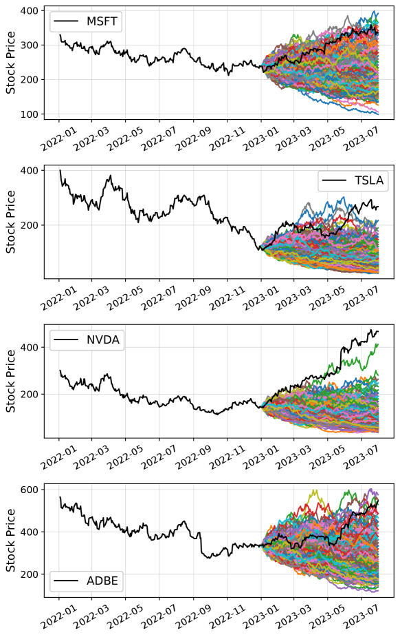
Figure 2: Example of Real Stock Prices in S&P 30 Versus Monte Carlo Simulated Sample Paths Using Generalized Lattice Model with Memory Length $m=5$.

Initializing the Multi-Double Linear Policies. As mentioned in previous sections, to implement the multi-double linear policies, one must specify the triple $(\alpha,w,v)$ and initial account value $V_{0}>0$. Here, we first take $\alpha=1/2$, an initial account value of $V_{0}=\$1$, and equal asset weights $w_{i}=\omega\in[0,1]$ for all $i=1,2,\dots,30$ for S&P 30, using a generalized lattice model with varying memory lengths $m\in\{1,2,5,10\}$ and a zero risk-free rate of $r_{f}=0$. For the specification of the initial allocation vector $v$, we consider three distinct strategies: The first one is equal-weighted allocation, denoted as $v_{EW}=[1/30\;\cdots\;1/30]^{\top}$. The second one is capital-weighted allocation, computed by the normalized weight of the S&P 30 index, denoted as $v_{{\rm CW}}$. The third one is gain-loss-weighted allocation, calculated using the gain-loss of training data as a criterion for capital allocation. It is denoted as $v_{GL,i}:=|S_{i}(k)/S_{i}(0)-1|/\sum_{i=1}^{n}|S_{i}(k)/S_{i}(0)-1|$, forming the vector $v_{\rm GL}$. Table 1 summarizes the choice of the relevant parameters.

Table 1: Summary of Parameters Sets.

	$(i)$	$(ii)$	$(iii)$
$V_{0}~{}(\$)$	1	1	1
$r_{f}~{}(\%)$	0	0	{0.92, 1.51, 3.88}
$m$	{1, 2, 5, 10}	1	1
$\alpha$	0.5	{0.1, 0.3, 0.5, 0.7, 0.9}	0.5
$w$	$\omega\in[0,1]$	$\omega\in[0,1]$	$\omega\in[0,1]$
$v$	$\{v_{\rm EW},v_{\rm CW},v_{\rm GL}\}$	$v_{\rm EW}$	$v_{\rm EW}$

Gain-Loss Analysis. With the various settings of the triple $(\alpha,w,v)$ as seen in Table 1, we implement the multi-double linear policies across the $30$ assets within the portfolio. The trading performance, as illustrated in Figure 3, depicts the average cumulative gain-loss against various weights for the parameter set $(i)$ in Table 1. We see that there exists a positive expected gain-loss $\overline{\mathcal{G}}(k)\geq 0$ for the given portfolio and for all parameter set combinations. Remarkably, this positivity is found to be robust across diverse choices of $v,w,m$ at $\alpha=1/2$.

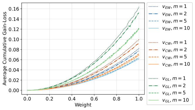
Figure 3: Average Cumulative Gain-Loss $\overline{\mathcal{G}}(k)$ Against Weights $\omega\in[0,1]$ for Parameter Set $(i)$ Described in Table 1.

Moreover, we present the associated standard deviation of the cumulative gain-loss for the parameter set $(i)$, depicted in Figure 4. Notably, both the average cumulative gain-loss and the corresponding standard deviation exhibit increasing monotonicity with respect to the weights, as shown in Figures 3 and 4. The results presented here form a foundation for practitioners aiming to explore novel trading paradigms; see Section 5.2 to follow.

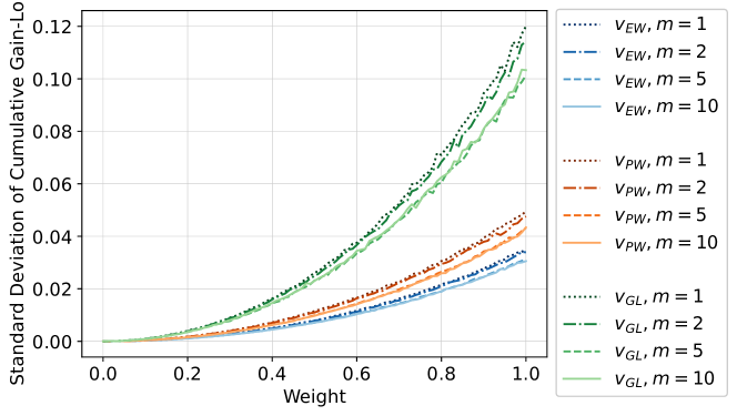
Figure 4: Standard Deviation of Cumulative Gain-Loss ${\rm std}(\mathcal{G}(k))$ Against Weights $\omega\in[0,1]$ for Parameter Set $(i)$ Specified in Table 1.

Example 5.2 (Sensitivity Analysis).

Continuing with the dataset and estimations provided in Example 5.1, we proceed further to analyze the gain-loss trading performance under different $\alpha\in\{0.1,0.3,0.5,0.7,0.9\}$, in combination with various weights $\omega$, as the parameter set $(ii)$ listed in Table 1. The corresponding results are shown in Figure 5. We see that the average gain-loss is positive for $\alpha\in\{0.1,0.3,0.5\}$, implying that there is a preference for initially allocating more capital to the short positions. In contrast, a negative average gain-loss is recorded for $\alpha\in\{0.7,0.9\}$. This phenomenon might be attributable to a decreasing trend for the S&P 30 over the examined period.

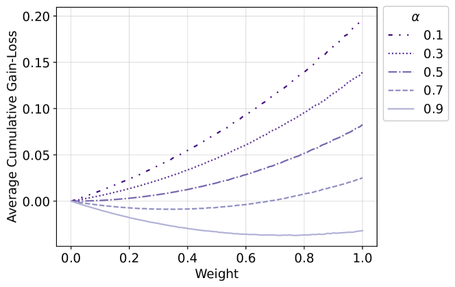
Figure 5: Sensitivity of $\alpha$: Average Cumulative Gain-Loss Versus Weights Under Different $\alpha$ Values.

Besides, we extend our analysis to implement multi-double linear policies that incorporate a non-zero risk-free rate, $r_{f}\in\{0.92\%,1.51\%,3.88\%$}, as outlined in the parameter set $(iii)$ in Table 1. By comparing the performances under parameter set $(i)$ with $v_{EW}$, $m=1$ versus $(iii)$, represented respectively in Figure 6, we observe that incorporating a risk-free rate for long positions leads to a higher cumulative gain-loss, which is consistent with the intuition that the risk-free rate would contribute additional capital due to under-investment in each period.

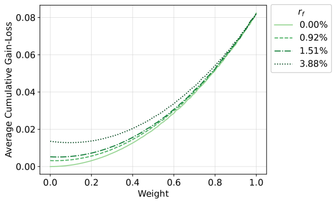
Figure 6: Sensitivity of $r_{f}$: Average Cumulative Gain-Loss Versus Weight Under Different Risk-Free Rates.

5.2 Out-of-Sample Trading Performance with Costs

This section studies out-of-sample trading performance using the multi-double linear policies with triple $(\alpha,w,v)\in\{1/2\}\times[0,1]^{n}\times\mathcal{V}$. In the following analysis, we also consider the impact of transaction costs.

5.2.1 Identifying Optimal Weights via Mean-Variance Efficient Frontier

When the weight $w_{i}=\omega$ for all $i=1,\dots,n$, Figure 3 reveals that the expected cumulative gain-loss increases as the weight $\omega$ increases. This is also evident in the standard deviation of the cumulative gain-loss across different weights; see Figure 4. Therefore, we then depict the mean-variance efficient frontiers using the expected cumulative gain-loss $\overline{\mathcal{G}}(k)$ against the standard deviation ${\rm std}(\mathcal{G}(k))$, as shown in Figure 7. Based on the monotonic increasing property, one can determine an optimal weight, call it $w^{*}$, using the mean-variance approach outlined in hsieh2022robust.

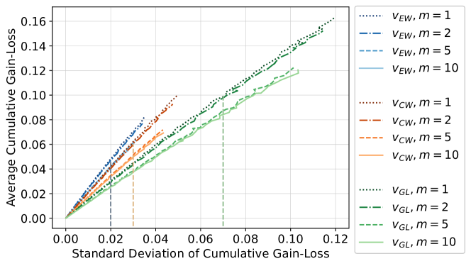
Figure 7: Mean-Standard Deviation Efficient Frontiers: Expected Cumulative Gain-Loss $\overline{\mathcal{G}}(k)$ Against Standard Deviation ${\rm std}(\mathcal{G}(k))$ for Parameter Set $(i)$.

In particular, the procedure is as follows: We begin by specifying a target standard deviation, then identify the corresponding maximum expected gain-loss under the chosen target. Once this maximum expected gain-loss is decided, it can be traced back to the optimal weight due to the strictly increasing relationship between expected gain-loss and weight. Below we consider three different approaches to identifying optimal weights.

Constant Optimal Weight for S&P 30. Consider the same S&P 30 dataset from Example 5.1. Suppose we set the target standard deviation ${\rm std}(\mathcal{G}_{\rm EW}(k)):=0.02$, ${\rm std}(\mathcal{G}_{\rm CW}(k)):=0.03$, and ${\rm std}(\mathcal{G}_{\rm GL}(k)):=0.07$ for $v_{\rm EW}$, $v_{\rm CW}$, and $v_{\rm GL}$, respectively, represented by the dashed line in Figure 7, for the parameter set $(i)$ with memory length $m=1$. The maximum expected gain-loss are determined as $\overline{\mathcal{G}}_{\rm EW}(k)\approx 0.0479$, $\overline{\mathcal{G}}_{\rm CW}(k)\approx 0.0614$, and $\overline{\mathcal{G}}_{\rm GL}(k)\approx 0.0963$. Due to the strictly monotonic increasing relationship between expected gain-loss and weight $\omega$, as seen in Figure 3, we can readily trace back the optimal weight: $w^{*}_{c,\rm EW}\approx 0.77$, $w^{*}_{c,\rm CW}\approx 0.79$, and $w^{*}_{c,\rm GL}\approx 0.78$, collectively denoted as $w_{c}^{*}:=\{w^{*}_{c,\rm EW},w^{*}_{c,\rm CW},w^{*}_{c,\rm GL}\}$.

Optimal Weight Determined by Top 10 Companies of S&P 30. Except for assigning the same constant weight $w_{c}^{*}$ for all assets, an alternative approach focuses solely on investing assets that exhibit the most promising performance. Here, we consider allocating the optimal constant weights to the top 10 assets of S&P 30 that exhibit the highest gain-loss, as determined by the training data. For the remaining assets that are not selected, we assign weights of zero. The corresponding weight is denoted as $w_{\rm top}^{*}$.

Optimal Weight Determined by Each Company. Lastly, we explore determining optimal weights for individual assets, denoted by $w_{i}^{*}$ for $i=1,\dots,n$, using the monotonic increasing property between gain-loss function and weight. For instance, by setting a uniform target standard deviation ${\rm std}(\mathcal{G}(k)):=0.01$ for all assets, represented by the dashed line shown in Figure 8, we can determine the associated maximum average cumulative gain-loss for each asset, leading to a set of optimal weights called $w_{\rm vary}^{*}:=\{w_{i}^{*}\}$ via a similar method mentioned previously.

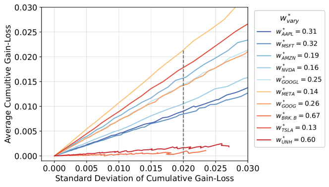
Figure 8: Mean-Variance Efficient Frontiers: Average Cumulative Gain-Loss $\overline{\mathcal{G}}_{i}(k)$ Against Standard Deviation ${\rm std}(\mathcal{G}_{i}(k))$ for top 10 Asset in S&P 30 Portfolio.

5.2.2 Out-of-Sample Trading Performance via Backtesting

With the selected optimal weights obtained in the preceding sections, we conducted backtesting over an out-of-sample period from January 2023 to July 2023. To analyze the trading performance across distinct sets of triple parameters $(\alpha,w,v)$, we carry out three initial allocations $v\in\{v_{\rm EW},v_{\rm CW},v_{\rm GL}\}$ and three types of optimal weights $w\in\{w_{c}^{*},w_{\rm top}^{*},w_{\rm vary}^{*}\}$, the constant optimal weight, the top 10 constant optimal weight, and the optimal weight varying among assets, respectively at $\alpha=1/2$. The corresponding trading trajectories and performance are shown in Figure 9 and quantitatively summarized in Table 2. For these scenarios, we incorporate a non-zero risk-free rate $r_{f}=3.88\%$ and a transaction cost $c=0.01\%$, corresponding to 1 basis point, for multi-double linear policies.

Due to the explicit trend for the year 2023 for some assets listed in S&P 30, the multi-double linear policies assure positive gain-loss for several parameter sets even in the consideration of transaction costs. Additionally, the triple $(\alpha,w,v)=(1/2,w_{\rm top}^{*},v_{\rm GL})$ has maximium out-of-sample gain-loss, $(1/2,w_{\rm top}^{*},v_{\rm EW})$ has minimum standard deviation, and $(1/2,w_{\rm vary}^{*},v_{\rm GL})$ has minimum maximum percentage drawdown.

Additionally, Figure 9 also presents Monte-Carlo-based 95% prediction intervals for each trading scenario in the figure. These intervals were generated via 10,000 simulated prices within the framework of the generalized lattice market model. For each path, we compute the average gain-loss and standard deviation for each day. In the figure, three distinct prediction intervals are highlighted. The dark-gray, gray, and light-gray regions correspond to the parameter triples $(1/2,w_{\rm top}^{*},\cdot)$, $(1/2,w_{\rm c}^{*},\cdot)$, and $(1/2,w_{\rm vary}^{*},\cdot)$, respectively. These intervals exhibit significant positive gain-loss regions, which is consistent with our theory.

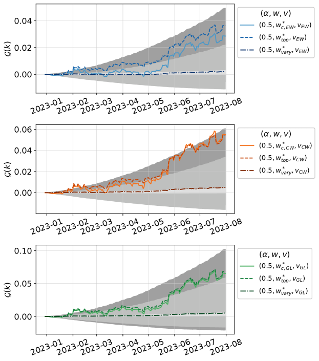
Figure 9: Gain-Loss Trajectories under Multi-Double Linear Policies: The figure depicts the impact of various triple set parameters and transaction costs on the trajectories. Three distinct Monte-Carlo-based 95% prediction intervals are highlighted: the dark-gray region corresponds to the triple $(1/2,w_{\rm top}^{*},\cdot)$, the gray region to the triple $(1/2,w_{\rm c}^{*},\cdot)$, and the light-gray region to the triple $(1/2,w_{\rm vary}^{*},\cdot)$.

Table 2: Out-of-Sample Trading Performance of Multi-Double Linear Policies with Various Triples (Best Performance in Each Column Denoted in Bold.

$(\alpha,w,v)$	Gain-Loss	Standard Deviation	Maximum Drawdown (%)
$(1/2,w_{c,\rm EW}^{*},v_{\rm EW})$	0.0286	0.0099	0.6675
$(1/2,w_{\rm top}^{*},v_{\rm EW})$	0.0364	0.0114	0.5964
$(1/2,w_{\rm vary}^{*},v_{\rm EW})$	0.0021	0.0007	0.0721
$(1/2,w_{c,\rm CW}^{*},v_{\rm CW})$	0.0549	0.0186	1.0352
$(1/2,w_{\rm top}^{*},v_{\rm CW})$	0.0540	0.0171	0.8278
$(1/2,w_{\rm vary}^{*},v_{\rm CW})$	0.0050	0.0016	0.0737
$(1/2,w_{c,\rm GL}^{*},v_{\rm GL})$	0.0654	0.0216	1.3483
$(1/2,w_{\rm top}^{*},v_{\rm GL})$	0.0683	0.0219	1.2969
$(1/2,w_{\rm vary}^{*},v_{\rm GL})$	0.0051	0.0016	0.0592

It is worth noting that the initial allocation for long and short positions, $\alpha$, influences the gain-loss performance; see Figure 5. As a result, we conduct the backtesting with varying $\alpha\in\{0.1,0.3,0.5,0.7,0.9\}$ as demonstrated in Figure 10. Our analysis reveals that a positive gain-loss is attained for $\alpha\in\{0.5,0.7,0.9\}$, while negative gain-loss is observed for $\alpha\in\{0.1,0.3\}$, considering a transaction cost of $0.01\%$ per trade and an annual risk-free rate of $r_{f}=3.88\%$. This phenomenon in gain-loss can be attributed to the bullish market trends present in the testing data for the year 2023.

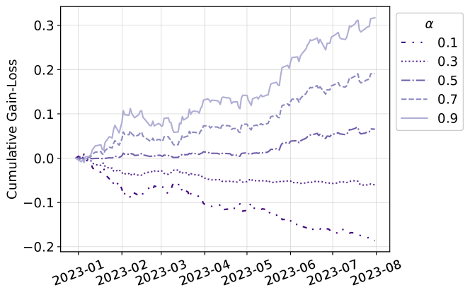
Figure 10: Cumulative Gain-Loss Trajectories with Varying $\alpha$.

6 Concluding Remark

In this paper, we investigated the stochastic robustness of a novel trading scheme called the multi-double linear policy within a generalized lattice market that accounts for both serially correlated returns and asset correlation. We proved that our policies assure survivability and probabilistic positivity. We derived a detailed gain-loss performance analysis, leading to the derivation of an analytic expression for the worst-case expected gain-loss and evidence that the proposed policies might sustain an “approximate” robust positive expected profit. Additionally, we proved sufficient conditions that multi-double linear policies can lead to positive expected profits if the market has a clear trend. This remarkable result holds true even within a symmetric lattice market. Through a conditional probabilistic model, we uncovered that the parameter space of our mode forms a convex polyhedron, estimated efficiently via a constrained least-squares method. Validated by extensive empirical studies with S&P 30 assets, we substantiate robust support for the theoretical findings.

As for future research, extending our analysis to the current findings to involve time-varying weights $w_{i}(k)$ with time-varying movement factors $u_{i}(k)$ and $d_{i}(k)$ or even a return model that takes multiple outcomes, e.g., state prices duffie2010dynamic, luenberger2013investment. We envision this extension may necessitate the development of innovative mathematical tools to navigate the highly nonlinear, stochastic, and correlated nature of such models. Additionally, the impact of transaction costs could be considered to embed into the model to enhance the practicality of the proposed trading policy; see hsieh2022robustness for an initial result along this line of research. Lastly, as the generalized lattice model fits well in a daily basis time scale, it is interesting to see if the model works well in high-frequency settings, such as tick-by-tick basis; see goldstein2022high.

Appendix A Technical Proofs of Sections 3 and 4

Proof of Lemma 3.1.

For $i=1,2,\dots,n$, Asset $i$ has per-period returns $X_{i}(j)\in\{u_{i},d_{i}\}$ with $-1<d_{i}<0<u_{i}<1$. Hence, the account value of the long position for the $i$th asset is given by

$$V_{i,L}(k)=\alpha V_{i,0}R_{i+}(k) =\alpha V_{i,0}\prod_{j=0}^{k-1}\left((1+r_{f})+w_{i}(X_{i}(j)-r_{f})\right)$$

$$\geq\alpha V_{i,0}\left((1+r_{f})+w_{i}(d_{i}-r_{f})\right)^{k}$$

$$\geq\alpha V_{i,0}\left((1+r_{f})-w_{i}(1+r_{f})\right)^{k}$$

$$=\alpha V_{i,0}\left((1+r_{f})(1-w_{i})\right)^{k}\geq 0,$$

where the last inequality hold since $w_{i}\in[0,1]$ and $V_{i,0}\geq 0$ and $r_{f}\geq 0.$ Similarly,

$$V_{i,S}(k) =(1-\alpha)V_{i,0}R_{i-}(k)\geq(1-\alpha)V_{i,0}\left(1-w_{i}\right)^{k}\geq 0.$$

Hence, it follows that $V(k)=\sum_{i=1}^{n}(V_{i,L}(k)+V_{i,S}(k))\geq 0$ for all $k$ with probability one. To complete the proof, we note that if $v_{i}>0$ for some $i$ and $w_{i}\in(0,1)$ and $\alpha\in(0,1)$, then  $V_{i,L}(k)$ and $V_{i,S}(k)$ are strictly positive. Hence, $V(k)>0$ for all $k$ with probability one. ∎

Proof of Lemma 3.1.

Fix $\theta\in[0,1]$. Note that, by Lemma 3.1, $V(k)>0$ for all $k$ with probability one. Observe that

$$\mathbb{E}\left[V(k)-\theta\mathbb{E}[V(k)]\right] \leq\mathbb{E}\left[(V(k)-\theta\mathbb{E}[V(k)])\cdot\mathbb{1}_{\{V(k)>\theta\mathbb{E}[V(k)]\}}\right]$$

$$\leq\mathbb{E}[(V(k)-\theta\mathbb{E}[V(k)])^{2}]^{1/2}\cdot\mathbb{P}(V(k)>\theta\mathbb{E}[V(k)])^{1/2}$$

where the last inequality holds by the Cauchy-Schwarz inequality. Hence, it follows that

$$\mathbb{P}(V(k)>\theta\mathbb{E}[V(k)]) \geq\frac{(\mathbb{E}\left[V(k)-\theta\mathbb{E}[V(k)]\right])^{2}}{\mathbb{E}[(V(k)-\theta\mathbb{E}[V(k)])^{2}]}$$

$$=\frac{(1-\theta)^{2}(\mathbb{E}\left[V(k)\right])^{2}}{\mathbb{E}[(V(k)-\theta\mathbb{E}[V(k)])^{2}]}.$$

Note that the denominator is

$$\mathbb{E}[(V(k)-\theta\mathbb{E}[V(k)])^{2}] =\mathbb{E}[(V(k)-\mathbb{E}[V(k)]+\mathbb{E}[V(k)]-\theta\mathbb{E}[V(k)])^{2}]$$

$$={\rm var}(V(k))+(1-\theta)^{2}(\mathbb{E}[V(k)])^{2}.$$

Therefore, we have

$$\mathbb{P}(V(k)>\theta\mathbb{E}[V(k)]) \geq\frac{(1-\theta)^{2}(\mathbb{E}\left[V(k)\right])^{2}}{{\rm var}(V(k))+(1-\theta)^{2}(\mathbb{E}[V(k)])^{2}},$$

and the proof is complete. ∎

Proof of Lemma 3.2.

The proof is elementary. Fix $w_{i}=0$ for all $i=1,2,\dots,n$. Note that $V(k)=\sum_{i=1}^{n}V_{i,0}\left(\alpha R_{i+}(k)+(1-\alpha)R_{i-}(k)\right)$ with $R_{i+}(k)=(1+r_{f})^{k}$ and $R_{i-}(k)=1$. Using the fact that $\sum_{i=1}^{n}v_{i}=1$, it follows that $V(k)=\sum_{i=1}^{n}V_{i,0}\left(\alpha(1+r_{f})^{k}+(1-\alpha)\right)=(\alpha(1+r_{f})^{k}+(1-\alpha))V_{0}.$ Hence, the cumulative trading gain-loss function becomes $\mathcal{G}(k)=V(k)-V_{0}=\alpha((1+r_{f})^{k}-1)V_{0}\geq 0$ for all $k$ where the last inequality hold since $\alpha\in[0,1]$ and $r_{f}\geq 0.$ ∎

Proof of Lemma 3.2.

By the law of total expectation, it can be computed by

$$p_{i}(k) =\mathbb{E}\left[\mathbb{1}_{\{X_{i}(k)=u_{i}\}}\right]$$

$$=\mathbb{E}\left[\mathbb{E}[\mathbb{1}_{\{X_{i}(k)=u_{i}\}}\mid X(k-1:k-m)]\right]$$

$$=\mathbb{E}\left[\mathbb{P}\left(X_{i}(k)=u_{i}\mid X(k-1:k-m)\right)\right]$$

$$=\mathbb{E}\left[\Phi_{i,0}+\sum_{j=1}^{m}\Phi_{i,j}X_{i}(k-j)+\sum_{\ell=1}^{n}\Gamma_{i,\ell}X_{\ell}(k-1)\right]$$

$$=\Phi_{i,0}+\sum_{j=1}^{m}\Phi_{i,j}\mathbb{E}\left[X_{i}(k-j)\right]+\sum_{\ell=1}^{n}\Gamma_{i,\ell}\mathbb{E}\left[X_{\ell}(k-1)\right],$$

for stage $k=0,1,\dots$. Using the fact that $\mathbb{E}[X_{i}(k-j)]=(u_{i}-d_{i})\cdot p_{i}(k-j)+d_{i}$ and the initial conditions $p_{i}(-j)=\frac{x_{i}(-j)-d_{i}}{u_{i}-d_{i}},$ for $j=1,2,\dots,m$, we then have the recursion for probability at stage $k=0,1,\dots$,

$$p_{i}(k) =\Phi_{i,0}+\sum_{j=1}^{m}\Phi_{i,j}[(u_{i}-d_{i})\cdot p_{i}({k-j})+d_{i}]+\sum_{\ell=1}^{n}\Gamma_{i,\ell}[(u_{\ell}-d_{\ell})\cdot p_{\ell}(k-1)+d_{\ell}],$$

which completes the proof. ∎

Proof of Lemma 3.2.

By Lemma 3.2, the per-period returns of Asset $i$ have Bernoulli distribution with time-varying probability $p_{i}(\cdot)$. Hence, the expectation of $\log(1+w_{i}X_{i}(j))$ for a single stage is given by $\mathbb{E}[\log(1+w_{i}X_{i}(j))]=\log(1+w_{i}u_{i})p_{i}(j)+\log(1+w_{i}d_{i})(1-p_{i}(j)).$ Hence, summing up $k$ stages yields

$$\sum_{j=0}^{k-1}\mathbb{E}[\log(1+w_{i}X_{i}(j))] =\sum_{j=0}^{k-1}\log(1+w_{i}u_{i})p_{i}(j)+\log(1+w_{i}d_{i})(1-p_{i}(j))$$

$$=\log(1+w_{i}u_{i})\sum_{j=0}^{k-1}p_{i}(j)+\log(1+w_{i}d_{i})\sum_{j=0}^{k-1}(1-p_{i}(j))$$

$$=\mathbb{E}[H_{i}(k)]\log(1+w_{i}u_{i})+(k-\mathbb{E}[H_{i}(k)])\log(1+w_{i}d_{i}),$$

where $\mathbb{E}[H_{i}(k)]:=\sum_{j=0}^{k-1}p_{i}(j)$ is the expected number of the return process of Asset $i$ that receives positive returns up to stage $k-1$. An almost identical proof would work for the short side, i.e.,

$$\sum_{j=0}^{k-1}\mathbb{E}[\log(1-w_{i}X_{i}(j))]=\mathbb{E}[H_{i}(k)]\log(1-w_{i}u_{i})+(k-\mathbb{E}[H_{i}(k)])\log(1-w_{i}d_{i}),$$

which completes the proof. ∎

Proof of Corollary 3.1.

To prove part $(i)$, we fix $k>1$. Noting that if $r_{f}>0$, it would increase the $\overline{\mathcal{G}}(k)$; hence, without loss of generality, we may restrict our attention to the case $r_{f}=0$ in the proof that follows. Begin by considering the case $\mathbb{E}[H_{i}(k)]=0$. We first compute the functions $\beta_{i}(\cdot)$ and $\gamma_{i}(\cdot)$ in Theorem 3.1; i.e., $\beta_{i}(k)=(1+w_{i}d_{i})^{k}$ and $\gamma_{i}(k)=(1-w_{i}d_{i})^{k}$ Substituting these two quantities to the lower bound for $\overline{\mathcal{G}}(k)$ in Theorem 3.1, we obtain $\overline{\mathcal{G}}(k)>\sum_{i=1}^{n}\frac{V_{i,0}}{2}\left((1+w_{i}d_{i})^{k}+(1-w_{i}d_{i})^{k}-2\right)>0$ where the last inequality holds by the facts that $V_{i,0}>0$ and $(1+z)^{k}+(1-z)^{k}>2$ for all $z\neq 0$ and all $k>1$. An almost identical proof would work for the case of $\mathbb{E}[H_{i}(k)]=k$. Indeed, in this case, it is readily verified that $\overline{\mathcal{G}}(k)>\sum_{i=1}^{n}\frac{V_{i,0}}{2}\left((1+w_{i}u_{i})^{k}+(1-w_{i}u_{i})^{k}-2\right)>0.$ To prove part $(ii)$, we note that for $\mathbb{E}[H_{i}(k)]\in(0,k)$ and take $(1+w_{i}u_{i})^{\mathbb{E}[H_{i}(k)]}(1+w_{i}d_{i})^{k-\mathbb{E}[H_{i}(k)]}+(1-w_{i}u_{i})^{\mathbb{E}[H_{i}(k)]}(1-w_{i}d_{i})^{k-\mathbb{E}[H_{i}(k)]}>2$ for all $i$. Applying Theorem 3.1, it is readily verified that $\overline{\mathcal{G}}(k)>0$ for all $k$ immediately. ∎

Proof of Lemma 3.2.

The strict convexity is established by invoking the second-order derivative test. That is, for any $\varepsilon>0$, $\frac{\partial^{2}}{\partial\varepsilon^{2}}\theta(\varepsilon)=a^{\varepsilon}(\log a)^{2}+b^{\varepsilon}(\log b)^{2}>0$ where the last inequality holds since $a,b>0$ with $a,b\neq 1$ and $(\log a)^{2}$ and $(\log b)^{2}>0.$ To complete the proof, we must find the minimum, call it $\varepsilon^{*}$. Indeed, the first-order condition leads to $\frac{\partial}{\partial\varepsilon}\theta(\varepsilon)=a^{\varepsilon}\log a+b^{\varepsilon}\log b\equiv 0.$ That is, $\varepsilon=\varepsilon^{*}$ is the minimum of $\phi(\varepsilon)$ if and only if $a^{\varepsilon^{*}}\log a+b^{\varepsilon^{*}}\log b=0$. Moreover, note that if $a>1$ and $b\in(0,1)$, then $a^{\varepsilon}$ is increasing and $b^{\varepsilon}$ is decreasing. This implies that the sum $\phi(\varepsilon)=a^{\varepsilon}+b^{\varepsilon}$ has a unique minimum $\varepsilon^{*}>0$. Likewise, if $a\in(0,1)$ and $b>1$, then $a^{\varepsilon}$ is decreasing and $b^{\varepsilon}$ is increasing, hence $\phi(\varepsilon)$ again has a unique minimum $\varepsilon^{*}>0.$ ∎

Proof of Corollary 3.4.

Fix $k>1$. Without loss of generality, we shall give proof for the case $\mathbb{E}[H_{i}(k)]>k/2$ as the methodology for proving another side follows an almost identical argument. Indeed, for $i\in\{1,2,\dots,n\}$, $\mathbb{E}[H_{i}(k)]>k/2$ implies that there exists a constant $\varepsilon_{i}\in(0,k/2)$ such that $\mathbb{E}[H_{i}(k)]=k/2+\varepsilon_{i}$. Now, take $\alpha=1/2$. Theorem 3.1 implies that the expected gain-loss function satisfies

$$\overline{\mathcal{G}}(k) >\sum_{i=1}^{n}\frac{V_{i,0}}{2}\left(\beta_{i}(k)+\gamma_{i}(k)-2\right),$$ (11)

where the two quantities $\beta_{i}(k)$ and $\gamma_{i}(k)$ satisfy

$$\beta_{i}(k) =(1+w_{i}u_{i})^{\mathbb{E}[H_{i}(k)]}(1+w_{i}d_{i})^{k-\mathbb{E}[H_{i}(k)]}$$

$$=(1+w_{i}u_{i})^{k/2+\varepsilon_{i}}(1+w_{i}d_{i})^{k-(k/2+\varepsilon_{i})}$$

$$=[(1+w_{i}u_{i})(1+w_{i}d_{i})]^{k/2}\left(\frac{1+w_{i}u_{i}}{1+w_{i}d_{i}}\right)^{\varepsilon_{i}}$$

and

$$\gamma_{i}(k) =(1-w_{i}u_{i})^{\mathbb{E}[H_{i}(k)]}(1-w_{i}d_{i})^{k-\mathbb{E}[H_{i}(k)]}$$

$$=(1-w_{i}u_{i})^{k/2+\varepsilon_{i}}(1-w_{i}d_{i})^{k-(k/2+\varepsilon_{i})}$$

$$=[(1-w_{i}u_{i})(1-w_{i}d_{i})]^{k/2}\left(\frac{1-w_{i}u_{i}}{1-w_{i}d_{i}}\right)^{\varepsilon_{i}}.$$

Since $u_{i}=-d_{i}$ for all $i$, it is readily verified that $\beta_{i}(k)=(1-w_{i}^{2}d_{i}^{2})^{k/2}\left(\frac{1-w_{i}d_{i}}{1+w_{i}d_{i}}\right)^{\varepsilon_{i}}$ and $\gamma_{i}(k)=(1-w_{i}^{2}d_{i}^{2})^{k/2}(\frac{1+w_{i}d_{i}}{1-w_{i}d_{i}})^{\varepsilon_{i}}.$ Substituting these into Inequality (11) yields

$$\overline{\mathcal{G}}(k) >\sum_{i=1}^{n}\frac{V_{i,0}}{2}\left([1-w_{i}^{2}d_{i}^{2}]^{k/2}\left[\left(\frac{1-w_{i}d_{i}}{1+w_{i}d_{i}}\right)^{\varepsilon_{i}}+\left(\frac{1-w_{i}d_{i}}{1+w_{i}d_{i}}\right)^{-\varepsilon_{i}}\right]-2\right)$$

which is desired.

Similarly, for the case $\mathbb{E}[H_{i}(k)]<k/2$ implies that there exists a constant $\varepsilon_{i}\in(0,k/2)$ such that $\mathbb{E}[H_{i}(k)]=k/2-\varepsilon_{i}$. Following the similar method, take $\alpha=1/2$ and $u_{i}=-d_{i}$, by Theorem 3.1, we have

$$\overline{\mathcal{G}}(k)\geq\sum_{i=1}^{n}\frac{V_{i,0}}{2}(\beta_{i}(k)+\gamma_{i}(k)-2),$$

where $\beta_{i}(k)=(1-w_{i}^{2}d_{i}^{2})^{k/2}\left(\frac{1-w_{i}d_{i}}{1+w_{i}d_{i}}\right)^{-\varepsilon_{i}}$ and $\gamma_{i}(k)=(1-w_{i}d_{i})^{k/2}\left(\frac{1+w_{i}d_{i}}{1-w_{i}d_{i}}\right)^{-\varepsilon_{i}}$. It follows that

$$\overline{\mathcal{G}}(k)>\sum_{i=1}^{n}\frac{V_{i,0}}{2}\left([1-w_{i}^{2}d_{i}^{2}]^{k/2}\left[\left(\frac{1-w_{i}d_{i}}{1+w_{i}d_{i}}\right)^{\varepsilon_{i}}+\left(\frac{1-w_{i}d_{i}}{1+w_{i}d_{i}}\right)^{-\varepsilon_{i}}\right]-2\right).$$

To prove part $(ii)$, take $\varepsilon_{i}=0$ in the proof above, then one immediately obtains $\overline{\mathcal{G}}(k)>\sum_{i=1}^{n}{V_{i,0}}\left([1-w_{i}^{2}d_{i}^{2}]^{k/2}-1\right)$ and the proof is complete. ∎

Proof of Lemma 3.3.

Fix $z>0$ with $z\neq 1$. An elementary calculus proof would work for verifying the strict increasingness of the function $\phi(\varepsilon)$. That is, $\phi^{\prime}(\varepsilon)=z^{\varepsilon}\log z-z^{-\varepsilon}\log z$. Proceeds with a proof by contradiction by assuming that the function was not strictly increasing. Then we have $z^{\varepsilon}\log z\leq z^{-\varepsilon}\log z.$ Equivalently

$$z^{2\varepsilon}\log z\leq\log z.$$ (12)

If $z>1$, then $\log z>0$. Hence Inequality (12) implies that $z^{2\varepsilon}\leq 1$ for $\varepsilon>0$, which is absurd since it contradicts $z>1$. On the other hand, if $z\in(0,1)$, then $\log z<0$. In this case, Inequality (12) becomes $z^{2\varepsilon}\geq 1$ for $\varepsilon>0$, which is again absurd. Therefore, $\phi^{\prime}(\varepsilon)>0$ for $\varepsilon>0$ and the function $\phi(\varepsilon)$ is a strictly increasing function. To complete the proof, invoking a usual limiting argument leads to $\inf\phi(\varepsilon)=2.$ ∎

Proof of Lemma 4.3.

For $i,\ell=1,\dots,n$ and $j=1,\dots,m$, we begin by re-expressing the products $\Phi_{i,j}u_{i}$, $\Phi_{i,j}d_{i}$, $\Gamma_{i,\ell}u_{\ell}$, and $\Gamma_{i,\ell}d_{\ell}$ as

$$\Phi_{i,j}u_{i} =\frac{u_{i}+d_{i}}{2}\Phi_{i,j}+\frac{u_{i}-d_{i}}{2}\Phi_{i,j};$$

$$\Phi_{i,j}d_{i} =\frac{u_{i}+d_{i}}{2}\Phi_{i,j}-\frac{u_{i}-d_{i}}{2}\Phi_{i,j};$$

$$\Gamma_{i,\ell}u_{\ell} =\frac{u_{\ell}+d_{\ell}}{2}\Gamma_{i,\ell}+\frac{u_{\ell}-d_{\ell}}{2}\Gamma_{i,\ell};$$

$$\Gamma_{i,\ell}d_{\ell} =\frac{u_{\ell}+d_{\ell}}{2}\Gamma_{i,\ell}-\frac{u_{\ell}-d_{\ell}}{2}\Gamma_{i,\ell}.$$

Hence, the conditions $0\leq\Phi_{i,0}+\sum_{j=1}^{m}\Phi_{i,j}x_{i}(k-j)+\sum_{\ell=1}^{n}\Gamma_{i,\ell}x_{\ell}(k-1)\leq 1$ with $x_{i}(k-j)\in\{u_{i},d_{i}\}$ holds if and only if

$$0\leq \Phi_{i,0}+\left(\frac{u_{i}+d_{i}}{2}\sum_{j=1}^{m}\Phi_{i,j}\right)\pm\frac{u_{i}-d_{i}}{2}\Phi_{i,1}\pm\frac{u_{i}-d_{i}}{2}\Phi_{i,2}\pm\dots\pm\frac{u_{i}-d_{i}}{2}\Phi_{i,m}$$

$$+\left(\sum_{\ell=1}^{n}\frac{u_{\ell}+d_{\ell}}{2}\Gamma_{i,\ell}\right)\pm\frac{u_{1}-d_{1}}{2}\Gamma_{i,1}\pm\frac{u_{2}-d_{2}}{2}\Gamma_{i,2}\pm\dots\pm\frac{u_{n}-d_{n}}{2}\Gamma_{i,n}\leq 1.$$

Therefore, it suffices to ensure that the following inequalities hold

$$0\leq\Phi_{i,0}+\frac{u_{i}+d_{i}}{2}\sum_{j=1}^{m}\Phi_{i,j}+\sum_{\ell=1}^{n}\frac{u_{\ell}+d_{\ell}}{2}\Gamma_{i,\ell}+\frac{u_{i}-d_{i}}{2}\sum_{j=1}^{m}\left|\Phi_{i,j}\right|+\sum_{\ell=1}^{n}\frac{u_{\ell}-d_{\ell}}{2}\left|\Gamma_{i,\ell}\right|\leq 1;$$

$$0\leq\Phi_{i,0}+\frac{u_{i}+d_{i}}{2}\sum_{j=1}^{m}\Phi_{i,j}+\sum_{\ell=1}^{n}\frac{u_{\ell}+d_{\ell}}{2}\Gamma_{i,\ell}-\frac{u_{i}-d_{i}}{2}\sum_{j=1}^{m}\left|\Phi_{i,j}\right|-\sum_{\ell=1}^{n}\frac{u_{\ell}-d_{\ell}}{2}\left|\Gamma_{i,\ell}\right|\leq 1.$$

Via a straightforward calculation, it follows that $\frac{u_{i}-d_{i}}{2}\sum_{j=1}^{m}\left|\Phi_{i,j}\right|+\sum_{\ell=1}^{n}\frac{u_{\ell}-d_{\ell}}{2}\left|\Gamma_{i,\ell}\right|\leq\frac{1}{2}$ and

$$-\frac{1}{2}+\frac{u_{i}-d_{i}}{2}\sum_{j=1}^{m}\left|\Phi_{i,j}\right|+\sum_{\ell=1}^{n}\frac{u_{\ell}-d_{\ell}}{2}\left|\Gamma_{i,\ell}\right| \leq\Phi_{i,0}-\frac{1}{2}+\frac{u_{i}+d_{i}}{2}\sum_{j=1}^{m}\Phi_{i,j}+\sum_{\ell=1}^{n}\frac{u_{\ell}+d_{\ell}}{2}\Gamma_{i,\ell}$$

$$\leq\frac{1}{2}-\frac{u_{i}-d_{i}}{2}\sum_{j=1}^{m}\left|\Phi_{i,j}\right|-\sum_{\ell=1}^{n}\frac{u_{\ell}-d_{\ell}}{2}\left|\Gamma_{i,\ell}\right|.$$

These conditions can be written as

$$\left|\Phi_{i,0}-\frac{1}{2}+\frac{u_{i}+d_{i}}{2}\sum_{j=1}^{m}\Phi_{i,j}+\sum_{\ell=1}^{n}\frac{u_{\ell}+d_{\ell}}{2}\Gamma_{i,\ell}\right|+\frac{u_{i}-d_{i}}{2}\sum_{j=1}^{m}\left|\Phi_{i,j}\right|+\sum_{\ell=1}^{n}\frac{u_{\ell}-d_{\ell}}{2}\left|\Gamma_{i,\ell}\right|\leq\frac{1}{2}.$$

To complete the proof, we note that the inequalities are linear in $\Phi_{i,j}$ and $\Gamma_{i,\ell}$, which forms a convex polyhedron. ∎

Appendix B Estimated Parameters of the S&P 30 Stocks

This appendix summarizes the estimated parameters for the S&P 30 stocks used in Section 5. Table 3 include the estimated movement factors $\widehat{U}$ and $\widehat{D}$, Tables 4 to 7 summarize the estimated serial correlation coefficients $\Phi_{i,j}$ with various memory length $m\in\{1,2,5,10\}$, and Table 8 record the asset correlation coefficient matrix $\Gamma$. In the following tables, the symbol “mean” refers to the average of the data and“std” refers to the standard deviation of the data.

Table 3: Estimated $\widehat{U}$ and $\widehat{D}$.

	$\widehat{U}$	$\widehat{D}$
AAPL	0.0173	-0.0175
ABBV	0.0101	-0.0109
ADBE	0.0207	-0.0212
AMZN	0.0229	-0.0242
AVGO	0.0187	-0.0182
BAC	0.0165	-0.0146
BRK.B	0.0112	-0.0108
COST	0.0138	-0.0143
CSCO	0.0136	-0.0129
CVX	0.0158	-0.0163
GOOG	0.0183	-0.0190
GOOGL	0.0188	-0.0188
HD	0.0146	-0.0153
JNJ	0.0088	-0.0080
JPM	0.0149	-0.0142
KO	0.0086	-0.0099
LLY	0.0141	-0.0127
MA	0.0156	-0.0152
MCD	0.0099	-0.0089
META	0.0249	-0.0299
MRK	0.0099	-0.0089
MSFT	0.0173	-0.0170
NVDA	0.0305	-0.0333
PEP	0.0088	-0.0092
PG	0.0101	-0.0107
TSLA	0.0291	-0.0349
UNH	0.0108	-0.0130
V	0.0144	-0.0143
WMT	0.0106	-0.0120
XOM	0.0174	-0.0175
mean	0.0156	-0.0161
std	0.0057	0.0069
min	0.0086	-0.0349
max	0.0305	-0.0080

Table 4: Estimated $\widehat{\Phi}_{i,j}$ for Memory Length $m=1$.

	$\widehat{\Phi}_{i,0}$	$\widehat{\Phi}_{i,1}$
AAPL	0.4743	-7.0577
ABBV	0.5648	-3.3926
ADBE	0.4675	-4.5233
AMZN	0.4637	-3.1458
AVGO	0.4934	-7.1075
BAC	0.4425	-1.7751
BRK.B	0.5066	-8.0508
COST	0.4891	-5.7026
CSCO	0.4554	-6.9281
CVX	0.5713	-0.4806
GOOG	0.4617	-6.5382
GOOGL	0.4505	-7.0812
HD	0.4898	-4.4559
JNJ	0.4915	-4.9624
JPM	0.4778	-4.6107
KO	0.5666	-6.6020
LLY	0.5287	-0.5153
MA	0.5037	-7.0355
MCD	0.4806	-10.0977
META	0.4717	-3.4837
MRK	0.5634	-2.5778
MSFT	0.4679	-8.2390
NVDA	0.4914	-2.0229
PEP	0.5407	-9.1421
PG	0.5140	-5.9338
TSLA	0.4901	-1.3042
UNH	0.5670	-9.1984
V	0.5042	-5.5996
WMT	0.5403	-2.6996
XOM	0.5775	0.2417
mean	0.5036	-5.0007
std	0.0406	2.8112
min	0.4425	-10.0977
max	0.5775	0.2417

Table 5: Estimated $\widehat{\Phi}_{i,j}$ for Memory Length $m=2$.

	$\widehat{\Phi}_{i,0}$	$\widehat{\Phi}_{i,1}$	$\widehat{\Phi}_{i,2}$
AAPL	0.4724	-6.8957	-3.2137
ABBV	0.5710	-3.2523	-4.3757
ADBE	0.4676	-4.5708	-1.2987
AMZN	0.4637	-2.9836	-0.9418
AVGO	0.4922	-7.0590	-0.2977
BAC	0.4406	-1.9511	0.2551
BRK.B	0.5054	-8.0853	-3.9996
COST	0.4909	-5.8565	-0.9620
CSCO	0.4562	-7.0756	-1.4489
CVX	0.5732	-0.4694	-1.8346
GOOG	0.4608	-6.3603	-1.6429
GOOGL	0.4480	-6.9173	-2.4574
HD	0.4849	-4.1834	-4.1064
JNJ	0.4939	-4.7201	-1.8473
JPM	0.4776	-4.8785	3.6627
KO	0.5656	-6.7373	-1.6632
LLY	0.5304	-0.7643	0.8080
MA	0.5017	-7.1727	0.0707
MCD	0.4822	-9.7406	2.5554
META	0.4649	-3.4820	-2.1993
MRK	0.5651	-2.7137	-1.9016
MSFT	0.4675	-8.3801	-2.6249
NVDA	0.4920	-1.8762	-0.6963
PEP	0.5398	-9.0190	-1.0837
PG	0.5130	-5.7470	2.9805
TSLA	0.4904	-1.2043	-0.5430
UNH	0.5691	-9.0458	-0.0528
V	0.5021	-5.6236	-1.9024
WMT	0.5427	-2.9355	0.0720
XOM	0.5773	0.1968	-0.4443
mean	0.5034	-4.9835	-1.0378
std	0.0417	2.7656	1.8998
min	0.4406	-9.7406	-4.3757
max	0.5773	0.1968	3.6627

Table 6: Estimated $\widehat{\Phi}_{i,j}$ for Memory Length $m=5$.

	$\widehat{\Phi}_{i,0}$	$\widehat{\Phi}_{i,1}$	$\widehat{\Phi}_{i,2}$	$\widehat{\Phi}_{i,3}$	$\widehat{\Phi}_{i,4}$	$\widehat{\Phi}_{i,5}$
AAPL	0.4903	-6.0457	-2.5566	1.3849	-0.5490	1.6469
ABBV	0.5774	-3.4784	-4.6048	-3.4273	-0.1246	-0.1277
ADBE	0.4706	-4.7356	-1.6543	1.4729	-1.5489	-1.0536
AMZN	0.4670	-3.0835	-0.9198	-0.2644	-2.0204	1.5314
AVGO	0.4960	-7.2420	-0.4197	-0.1947	-0.0650	-1.7599
BAC	0.4369	-1.8106	0.3323	-0.0738	-1.6913	1.8038
BRK.B	0.4974	-8.8585	-4.9791	0.6956	-1.9145	-2.2998
COST	0.4967	-6.3076	-1.1686	-1.8999	-2.6737	4.0319
CSCO	0.4513	-7.2763	-1.2937	2.1238	-1.5100	-1.8733
CVX	0.5620	-0.8948	-2.0258	-0.1786	1.8117	1.7782
GOOG	0.4666	-6.5287	-1.5938	-0.3628	-2.0394	0.5425
GOOGL	0.4657	-6.4507	-1.9203	0.0000	-2.2459	0.0000
HD	0.4913	-4.2705	-4.1762	0.3816	0.6885	0.5236
JNJ	0.4866	-4.9292	-2.8317	3.0761	3.2063	10.3256
JPM	0.4720	-4.8995	4.0073	0.3229	-1.6667	-1.8565
KO	0.5686	-7.1570	-1.5807	-0.7660	-1.9007	-0.2845
LLY	0.5337	-0.8408	0.9450	-0.6955	-3.2962	2.9291
MA	0.5069	-7.3545	0.1202	0.5930	0.2353	0.3416
MCD	0.4828	-9.5574	2.9993	-3.3113	2.2448	6.0217
META	0.4621	-3.4509	-2.1904	-0.3271	-0.8298	0.0918
MRK	0.5669	-2.1407	-2.0788	-2.3531	3.5751	-3.9520
MSFT	0.4835	-7.6361	-1.9472	-0.6301	0.0000	-1.7776
NVDA	0.4882	-1.9375	-0.4615	-1.1027	-1.0826	0.1271
PEP	0.5364	-10.4331	-1.7617	-2.7711	-5.2843	-3.3639
PG	0.5139	-5.5992	3.3013	-2.0523	2.6299	-2.4837
TSLA	0.4904	-1.3581	-0.5920	-0.4209	0.4666	-1.3029
UNH	0.5779	-9.8296	-0.6249	-1.8474	-0.2913	-0.2166
V	0.5070	-5.8935	-1.8933	-0.5778	-1.7258	0.2817
WMT	0.5407	-2.3627	-0.1161	0.7031	-2.0813	0.8319
XOM	0.5644	-0.1731	-0.7313	0.3908	2.1484	1.0343
mean	0.5050	-5.0845	-1.0806	-0.4037	-0.5845	0.3830
std	0.0402	2.8674	2.0398	1.5045	2.0326	2.8278
min	0.4369	-10.4331	-4.9791	-3.4273	-5.2843	-3.9520
max	0.5779	-0.1731	4.0073	3.0761	3.5751	10.3256

Table 7: Estimated $\widehat{\Phi}_{i,j}$ for Memory Length $m=10$.

	$\widehat{\Phi}_{i,0}$	$\widehat{\Phi}_{i,1}$	$\widehat{\Phi}_{i,2}$	$\widehat{\Phi}_{i,3}$	$\widehat{\Phi}_{i,4}$	$\widehat{\Phi}_{i,5}$	$\widehat{\Phi}_{i,6}$	$\widehat{\Phi}_{i,7}$	$\widehat{\Phi}_{i,8}$	$\widehat{\Phi}_{i,9}$	$\widehat{\Phi}_{i,10}$
AAPL	0.4867	-6.0468	-2.3184	1.0992	0.0000	1.1757	0.0000	0.0000	0.0000	0.0000	-1.3424
ABBV	0.5722	-3.0746	-4.3332	-3.2077	-0.2310	-0.0760	-0.0477	0.2086	1.7399	0.6545	-2.9690
ADBE	0.4714	-4.3141	-1.1528	1.1536	-1.1368	-0.3080	0.0000	0.0000	-1.6589	-0.8618	-0.6552
AMZN	0.4787	-2.8012	-0.4456	-0.3153	-1.9531	1.3428	0.0000	-0.7664	-0.8991	0.7221	1.0201
AVGO	0.5082	-6.5873	0.0000	0.0000	0.0000	-1.1906	-3.3023	0.0000	-0.8407	-0.6345	-0.6275
BAC	0.4393	-1.3490	-0.0889	-0.0362	-1.2976	2.2879	-2.7961	0.6335	-2.9673	1.7658	0.1447
BRK.B	0.4964	-8.6050	-4.4898	0.0000	-1.2611	-2.0547	-0.0023	1.7707	-0.7803	1.3104	1.4179
COST	0.5027	-6.3884	-0.6677	-1.7687	-2.6611	3.6459	1.0455	-0.5666	1.2112	0.5117	1.1456
CSCO	0.4658	-7.1298	-1.0377	2.5167	-0.0741	-0.5531	-1.2505	2.3559	-0.0075	2.6266	-0.4315
CVX	0.5627	-0.4194	-2.1235	-0.1231	1.8365	1.8130	-2.0245	2.6408	-2.5675	1.7544	-0.6850
GOOG	0.4672	-6.1960	-1.3498	0.0000	-1.7443	0.5515	-0.0591	0.0000	-0.0387	0.1627	0.9563
GOOGL	0.4602	-6.3070	-1.8457	0.0000	-2.1501	0.0000	0.0000	0.0000	0.0000	0.0000	0.0190
HD	0.5025	-4.7400	-4.6531	-0.3289	0.2936	0.4028	-0.5937	1.3441	1.0331	2.0433	2.1760
JNJ	0.5006	-5.7181	-3.9292	3.4345	2.8180	11.8124	0.1560	-0.5695	-2.5858	0.3663	-5.4969
JPM	0.4785	-4.5622	3.2834	0.2067	-0.6562	-1.5361	-0.1417	0.5352	0.7523	3.2933	-2.8566
KO	0.5604	-7.5233	-1.6110	-1.0146	-2.1853	0.0297	-6.1188	2.9035	0.9533	0.0414	-0.2377
LLY	0.5350	-0.8946	1.2286	0.2687	-3.6011	3.1966	0.0389	-1.2349	-3.2674	4.8204	-0.4896
MA	0.5014	-8.0033	-0.1182	0.5164	0.9363	0.7731	0.0000	-1.4314	-2.9440	-0.7316	0.3741
MCD	0.4984	-9.4845	1.8615	-2.3841	1.0978	3.7620	3.7078	2.8442	-3.3899	0.6593	3.6118
META	0.4688	-3.3157	-1.8679	-0.5192	-0.7732	0.3499	-1.1460	1.1556	0.6323	0.0000	-0.8245
MRK	0.5501	-2.8590	-1.1644	-2.1002	2.6720	-3.5841	0.2096	0.0355	6.0822	2.8016	1.7149
MSFT	0.4826	-7.4980	-1.6388	-0.1095	0.0000	-1.1698	-1.2919	0.0000	0.0000	0.2375	0.0000
NVDA	0.4831	-1.7214	-0.4927	-1.0516	-1.1298	0.2661	-0.4853	0.8280	-0.8354	-0.3877	0.3978
PEP	0.5298	-10.4575	-0.7566	-1.9033	-5.1067	-2.7873	-3.3101	2.0992	-0.1821	0.4434	-2.7524
PG	0.5165	-5.5333	2.5618	-1.9286	3.3486	-2.7486	-0.2179	-0.9519	-1.0760	0.8461	-0.0148
TSLA	0.4973	-0.8211	-0.5040	-0.2528	0.6465	-1.2883	0.3078	2.3891	-1.4361	1.4047	-0.8947
UNH	0.5718	-8.7663	-0.0536	-0.7555	0.0000	0.0000	-1.1147	0.1035	0.0000	1.7695	-6.8970
V	0.5082	-6.2467	-1.6439	-0.7032	-1.6754	0.0739	-1.0217	-1.6165	-0.7638	-2.4145	-1.9267
WMT	0.5482	-2.2058	-0.5936	0.9173	-2.7262	0.9771	-0.7612	0.1939	1.1571	-1.2646	3.2698
XOM	0.5674	0.5619	-0.4573	0.3952	2.2481	1.3658	-2.9903	2.7908	0.6023	1.5257	-2.6165
mean	0.5071	-4.9669	-1.0134	-0.2665	-0.4822	0.5510	-0.7737	0.5898	-0.4026	0.7822	-0.5157
std	0.0368	2.9305	1.8586	1.3714	1.9466	2.7760	1.7149	1.3465	1.8901	1.4626	2.2513
min	0.4393	-10.4575	-4.6531	-3.2077	-5.1067	-3.5841	-6.1188	-1.6165	-3.3899	-2.4145	-6.8970
max	0.5722	0.5619	3.2834	3.4345	3.3486	11.8124	3.7078	2.9035	6.0822	4.8204	3.6118

Table 8: Estimated Correlation Matrix $\widehat{\Gamma}$.

	AAPL	ABBV	ADBE	AMZN	AVGO	BAC	BRK.B	COST	CSCO	CVX	GOOG	GOOGL	HD	JNJ	JPM	KO	LLY	MA	MCD	META	MRK	MSFT	NVDA	PEP	PG	TSLA	UNH	V	WMT	XOM
AAPL	0	.24	.71	.70	.76	.57	.69	.63	.64	.29	.79	.80	.60	.37	.55	.52	.36	.75	.51	.59	.28	.82	.76	.55	.46	.64	.49	.70	.34	.28
ABBV	-	0	.18	.21	.26	.30	.41	.30	.31	.16	.22	.22	.28	.51	.35	.42	.51	.28	.32	.10	.49	.28	.19	.43	.44	.06	.51	.30	.25	.18
ADBE	-	-	0	.65	.71	.42	.52	.54	.54	.22	.72	.73	.61	.20	.43	.35	.30	.66	.37	.60	.15	.77	.72	.39	.33	.50	.29	.62	.27	.20
AMZN	-	-	-	0	.66	.55	.57	.56	.48	.31	.72	.72	.57	.23	.50	.36	.27	.60	.34	.61	.16	.74	.71	.36	.24	.59	.32	.55	.30	.25
AVGO	-	-	-	-	0	.56	.62	.57	.66	.30	.73	.74	.59	.25	.56	.42	.32	.67	.44	.56	.18	.76	.83	.43	.39	.59	.41	.61	.22	.27
BAC	-	-	-	-	-	0	.71	.41	.50	.36	.54	.54	.43	.31	.90	.44	.25	.60	.47	.42	.26	.56	.55	.40	.36	.41	.42	.59	.23	.31
BRK.B	-	-	-	-	-	-	0	.55	.60	.47	.62	.63	.57	.48	.71	.62	.43	.65	.50	.43	.37	.64	.58	.55	.46	.41	.49	.62	.36	.43
COST	-	-	-	-	-	-	-	0	.54	.23	.57	.57	.65	.41	.42	.56	.36	.49	.49	.37	.21	.61	.56	.58	.54	.46	.50	.48	.59	.20
CSCO	-	-	-	-	-	-	-	-	0	.25	.57	.57	.52	.41	.53	.55	.43	.54	.50	.42	.33	.59	.55	.55	.51	.36	.44	.51	.36	.21
CVX	-	-	-	-	-	-	-	-	-	0	.26	.26	.17	.12	.30	.19	.20	.24	.13	.19	.20	.26	.28	.15	0	.17	.25	.21	.20	.88
GOOG	-	-	-	-	-	-	-	-	-	-	0	1	.56	.27	.51	.37	.32	.66	.40	.68	.23	.85	.77	.41	.34	.55	.39	.59	.31	.21
GOOGL	-	-	-	-	-	-	-	-	-	-	-	0	.56	.27	.51	.38	.32	.66	.41	.68	.23	.85	.77	.42	.35	.55	.40	.60	.31	.22
HD	-	-	-	-	-	-	-	-	-	-	-	-	0	.38	.48	.51	.38	.57	.43	.48	.25	.62	.57	.52	.47	.35	.39	.54	.41	.14
JNJ	-	-	-	-	-	-	-	-	-	-	-	-	-	0	.35	.57	.60	.30	.48	.16	.64	.32	.18	.59	.59	.10	.55	.31	.33	.09
JPM	-	-	-	-	-	-	-	-	-	-	-	-	-	-	0	.46	.31	.60	.52	.39	.29	.53	.53	.43	.39	.37	.44	.58	.23	.28
KO	-	-	-	-	-	-	-	-	-	-	-	-	-	-	-	0	.43	.50	.63	.22	.42	.46	.34	.84	.75	.23	.54	.50	.43	.18
LLY	-	-	-	-	-	-	-	-	-	-	-	-	-	-	-	-	0	.38	.45	.29	.59	.38	.28	.47	.37	.19	.56	.41	.24	.18
MA	-	-	-	-	-	-	-	-	-	-	-	-	-	-	-	-	-	0	.55	.53	.29	.73	.68	.49	.44	.47	.42	.93	.26	.27
MCD	-	-	-	-	-	-	-	-	-	-	-	-	-	-	-	-	-	-	0	.23	.43	.47	.41	.68	.57	.25	.50	.53	.34	.13
META	-	-	-	-	-	-	-	-	-	-	-	-	-	-	-	-	-	-	-	0	.22	.63	.61	.28	.24	.39	.18	.46	.18	.14
MRK	-	-	-	-	-	-	-	-	-	-	-	-	-	-	-	-	-	-	-	-	0	.25	.10	.45	.45	.02	.50	.30	.23	.19
MSFT	-	-	-	-	-	-	-	-	-	-	-	-	-	-	-	-	-	-	-	-	-	0	.79	.49	.44	.55	.46	.66	.32	.22
NVDA	-	-	-	-	-	-	-	-	-	-	-	-	-	-	-	-	-	-	-	-	-	-	0	.35	.29	.67	.35	.62	.23	.23
PEP	-	-	-	-	-	-	-	-	-	-	-	-	-	-	-	-	-	-	-	-	-	-	-	0	.74	.22	.56	.48	.47	.16
PG	-	-	-	-	-	-	-	-	-	-	-	-	-	-	-	-	-	-	-	-	-	-	-	-	0	.15	.54	.43	.42	.03
TSLA	-	-	-	-	-	-	-	-	-	-	-	-	-	-	-	-	-	-	-	-	-	-	-	-	-	0	.28	.44	.17	.16
UNH	-	-	-	-	-	-	-	-	-	-	-	-	-	-	-	-	-	-	-	-	-	-	-	-	-	-	0	.41	.33	.22
V	-	-	-	-	-	-	-	-	-	-	-	-	-	-	-	-	-	-	-	-	-	-	-	-	-	-	-	0	.22	.24
WMT	-	-	-	-	-	-	-	-	-	-	-	-	-	-	-	-	-	-	-	-	-	-	-	-	-	-	-	-	0	.17
XOM	-	-	-	-	-	-	-	-	-	-	-	-	-	-	-	-	-	-	-	-	-	-	-	-	-	-	-	-	-	0

References

- Balvers and Mitchell (1997) Balvers RJ, Mitchell DW (1997) Autocorrelated Returns and Optimal Intertemporal Portfolio Choice. Management Science 43(11):1537–1551, URL http://dx.doi.org/10.1287/mnsc.43.11.1537.
- Barmish (2008) Barmish BR (2008) On Trading of Equities: A Robust Control Paradigm. IFAC Proceedings Volumes 41(2):1621–1626, URL http://dx.doi.org/10.3182/20080706-5-KR-1001.00276.
- Barmish and Primbs (2011) Barmish BR, Primbs JA (2011) On Arbitrage Possibilities via Linear Feedback in an Idealized Brownian Motion Stock Market. Proceedings of the IEEE Conference on Decision and Control (CDC) and European Control Conference (ECC), 2889–2894, URL http://dx.doi.org/10.1109/CDC.2011.6160731.
- Barmish and Primbs (2015) Barmish BR, Primbs JA (2015) On a New Paradigm for Stock Trading via a Model-Free Feedback Controller. IEEE Transactions on Automatic Control 61(3):662–676, URL http://dx.doi.org/10.1109/TAC.2015.2444078.
- Baumann (2016) Baumann MH (2016) On Stock Trading via Feedback Control when Underlying Stock Returns Are Discontinuous. IEEE Transactions on Automatic Control 62(6):2987–2992, URL http://dx.doi.org/10.1109/TAC.2016.2605743.
- Baumann (2023) Baumann MH (2023) On Theoretical Foundations of Mostly Model-Free Cross-Coupled Simultaneously Long-Short Stock Trading Controllers. European Journal of Control 100851, URL http://dx.doi.org/10.1016/j.ejcon.2023.100851.
- Baumann and Grüne (2019) Baumann MH, Grüne L (2019) Positive Expected Feedback Trading Gain for All Essentially Linearly Representable Prices. Proceedings of the Asian Control Conference (ASCC), 150–155.
- Boyd and Vandenberghe (2004) Boyd SP, Vandenberghe L (2004) Convex Optimization (Cambridge University Press).
- Campbell et al. (1993) Campbell JY, Grossman SJ, Wang J (1993) Trading Volume and Serial Correlation in Stock Returns. The Quarterly Journal of Economics 108(4):905–939.
- Casella and Berger (2001) Casella G, Berger RL (2001) Statistical Inference (Cengage Learning).
- Christoffersen and Diebold (2006) Christoffersen PF, Diebold FX (2006) Financial Asset Returns, Direction-of-Change Forecasting, and Volatility Dynamics. Management Science 52(8):1273–1287, URL http://www.jstor.org/stable/20110599.
- Cox et al. (1979) Cox JC, Ross SA, Rubinstein M (1979) Option Pricing: A Simplified Approach. Journal of Financial Economics 7(3):229–263, URL http://dx.doi.org/10.1016/0304-405X(79)90015-1.
- Cvitanic and Zapatero (2004) Cvitanic J, Zapatero F (2004) Introduction to the Economics and Mathematics of Financial Markets (MIT Press).
- Deshpande and Barmish (2018) Deshpande A, Barmish BR (2018) A Generalization of the Robust Positive Expectation Theorem for Stock Trading via Feedback Control. Proceedings of the European Control Conference (ECC), 514–520, URL http://dx.doi.org/10.1016/j.ifacol.2020.12.1249.
- Deshpande et al. (2020) Deshpande A, Gubner JA, Barmish BR (2020) On Simultaneous Long-Short Stock Trading Controllers with Cross-Coupling. IFAC-PapersOnLine 53(2):16989–16995, URL http://dx.doi.org/10.1016/j.ifacol.2020.12.1249.
- Dokuchaev (2002) Dokuchaev N (2002) Dynamic Portfolio Strategies: Quantitative Methods and Empirical Rules for Incomplete Information, volume 47 (Springer Science & Business Media).
- Dokuchaev and Savkin (1998) Dokuchaev N, Savkin A (1998) Asymptotic Arbitrage in a Stochastic Financial Market Model. Asymptotic Arbitrage in a Stochastic Financial Market Model, 100–104 (CESA’98 Conference Secretariat).
- Duffie (2010) Duffie D (2010) Dynamic Asset Pricing Theory (Princeton University Press).
- Fielitz (1971) Fielitz BD (1971) Stationarity of Random Data: Some Implications for the Distribution of Stock Price Changes. Journal of Financial and Quantitative Analysis 6(3):1025–1034, URL http://dx.doi.org/10.2307/2329918.
- Goldstein et al. (2022) Goldstein M, Kwan A, Philip R (2022) High-Frequency Trading Strategies. Management Science URL http://dx.doi.org/10.1287/mnsc.2022.4539.
- Granger and Hyung (2004) Granger CW, Hyung N (2004) Occasional Structural Breaks and Long Memory with an Application to the S&P 500 Absolute Stock Returns. Journal of Empirical Finance 11(3):399–421, URL http://dx.doi.org/10.1016/j.jempfin.2003.03.001.
- Hsieh (2022a) Hsieh CH (2022a) On Robust Optimal Linear Feedback Stock Trading. arXiv: 2202.02300 .
- Hsieh (2022b) Hsieh CH (2022b) On Robustness of Double Linear Trading with Transaction Costs. IEEE Control Systems Letters 7:679–684, URL http://dx.doi.org/10.1109/LCSYS.2022.3218541.
- Korajczyk and Sadka (2004) Korajczyk RA, Sadka R (2004) Are Momentum Profits Robust to Trading Costs? The Journal of Finance 59(3):1039–1082, URL https://www.jstor.org/stable/3694730.
- Luenberger (2013) Luenberger DG (2013) Investment Science (Oxford university press).
- Malekpour and Barmish (2016) Malekpour S, Barmish BR (2016) On Stock Trading Using a Controller with Delay: The Robust Positive Expectation Property. Proceedings of the IEEE Conference on Decision and Control (CDC), 2881–2887.
- Malekpour et al. (2018) Malekpour S, Primbs JA, Barmish BR (2018) A Generalization of Simultaneous Long–Short Stock Trading to PI Controllers. IEEE Transactions on Automatic Control 63(10):3531–3536, URL http://dx.doi.org/10.1109/TAC.2018.2799484.
- Maroni et al. (2019) Maroni G, Formentin S, Previdi F (2019) A Robust Design Strategy for Stock Trading via Feedback Control. Proceedings of the European Control Conference (ECC), 447–452.
- Officer (1972) Officer RR (1972) The Distribution of Stock Returns. Journal of the American Statistical Association 67(340):807–812, URL http://dx.doi.org/10.2307/2284641.
- O’Brien et al. (2020) O’Brien JD, Burke ME, Burke K (2020) A Generalized Framework for Simultaneous Long-Short Feedback Trading. IEEE Transactions on Automatic Control 66(6):2652–2663, URL http://dx.doi.org/10.1109/TAC.2020.3011914.
- Primbs and Barmish (2017) Primbs JA, Barmish BR (2017) On Robustness of Simultaneous Long-Short Stock Trading Control with Time-Varying Price Dynamics. IFAC-PapersOnLine 50(1):12267–12272, URL http://dx.doi.org/10.1016/j.ifacol.2017.08.2045.
- Primbs and Yamada (2018) Primbs JA, Yamada Y (2018) Pairs Trading under Transaction Costs using Model Predictive Control. Quantitative Finance 18(6):885–895, URL http://dx.doi.org/10.1080/14697688.2017.1374549.
- Tie et al. (2018) Tie J, Zhang H, Zhang Q (2018) An Optimal Strategy for Pairs Trading under Geometric Brownian Motions. Journal of Optimization Theory and Applications 179:654–675, URL http://dx.doi.org/10.1007/s10957-017-1065-8.
- Vitale (2018) Vitale P (2018) Robust Trading for Ambiguity-Averse Insiders. Journal of Banking & Finance 90:113–130, URL http://dx.doi.org/10.1016/j.jbankfin.2018.03.007.
- Wang and Hsieh (2023) Wang XY, Hsieh CH (2023) On Robustness of Double Linear Policy with Time-Varying Weights. Proceedings of the IEEE Conference on Decision and Control, forthcoming.
- Werner et al. (2023) Werner IM, Rindi B, Buti S, Wen Y (2023) Tick Size, Trading Strategies, and Market Quality. Management Science 69(7):3818–3837, URL http://dx.doi.org/doi.org/10.1287/mnsc.2022.4502.