Numerical simulation of time fractional Kudryashov-Sinelshchikov equation describing the pressure waves in a mixture of liquid and gas bubbles

Abstract

This article is concerned with an approximate analytical solution for the time-fractional Kudryashov-Sinelshchikov equation by using the reproducing kernel Hilbert space method. The main tools of this method are reproducing kernel theory, some important Hilbert spaces, the normal basis, orthogonalisation process, and homogenization. The effectiveness of reproducing kernel Hilbert space method is presented through the tables and graphs. These computational results indicate that this method is highly accurate and efficient for the time-fractional Kudryashov-Sinelshchikov equation. Also, it is demonstrated that the approximate solution uniformly converges to exact solution by using reproducing kernel Hilbert space method.

Keywords: Kudryashov-Sinelshchikov equation; RKHSM; Series solution.

Mathematics Subject Classification: 26A33, 35C10, 46E22, 46E40
PACS Numbers: 02.30.Jr

1 Introduction

In 2010, Kudryashov and Sinelshchikov noted a common non-linear partial differential equation for describing the pressure waves within a mixture of liquid and gas bubbles by considering the viscosity of liquid and heat transfer[1, 2] which is named as Kudryashov-Sinelshchikov equation (KSE). The time-fractional KSE of order $\alpha$ is considered as[3]

$$^{C}D^{\alpha}_{\tau}w(\zeta,\tau)+\gamma w(\zeta,\tau)w(\zeta,\tau)_{\zeta}+w(\zeta,\tau)_{\zeta\zeta\zeta}-(1+\beta)w(\zeta,\tau)_{\zeta}w(\zeta,\tau)_{\zeta\zeta}$$ (1.1)

$$-w(\zeta,\tau)w(\zeta,\tau)_{\zeta\zeta}-\nu w(\zeta,\tau)_{\zeta\zeta}-\mu w(\zeta,\tau)w(\zeta,\tau)_{\zeta\zeta}-\mu w(\zeta,\tau)^{2}=0,$$

$$(\zeta,\tau)\in\mathcal{D}=[a,b]\times[0,T],\ \ \alpha\in(0,1],$$

$$\begin{cases}w(\zeta,0)=f(\zeta),\\ w(a,\tau)=g_{1}(\tau),\\ w(b,\tau)=g_{2}(\tau),\end{cases}$$ (1.2)

where ${{}^{C}}{{D^{\alpha}}_{\tau}}$ denotes the Caputo derivative of order $\alpha$[4, 5, 6]. In the mentioned time-fractional KSE, $w$ is known to be density and $\beta,\gamma,\mu,\nu$ are real parameters. This equation is the generalization of the Burgers–Korteweg-de Vries (BKdV) equation and Korteweg-de Vries (KdV) equation. Many numerical and analytical methods are implemented for the study of KSE. Different methods such as Jacobi elliptic function method[7], Lie symmetry method[8], Improved $F$-expansion method[9], and multiple-expansion method[10] are used to find the exact solution of KSE.

The aim of this literature is to construct an approximate analytical solution for time-fractional KSE by using reproducing kernel Hilbert space method (RKHSM). Recently the theory of reproducing kernel emerged as a powerful framework in differential and integral equations, numerical analysis, and probability and statistics. RKHSM has many advantages, like (i) It does not need any discretization, i.e., this method is mesh-free. (ii) It provides a highly accurate approximate solution that converges to an exact solution[11, 12].

Different kinds of differential and integral equations, such as fractional Batru-type equations[13], fractional Baley-Trovik equation[14], Forced Duffing equation[15] with nonlocal boundary conditions, etc are studied under RKHSM to find accurate solutions of these equations.

To the best of the author’s knowledge, there are little literature that has obtained numerical solutions of the time-fractional KSE, and there is no research work for finding approximate analytical solution of the time-fractional KSE by using RKHSM. Hence in this literature, RKHSM is first time implemented on the time-fractional KSE where the fractional derivative is considered under Caputo sense.

This manuscript is organized as follows: Section 2 includes the mathematical preliminaries of RKHSM and reproducing kernel functions. In Section 3, RKHSM is applied to the time-fractional KSE equation. Convergence analysis and behavior of error is given in Section 4. In Section 5 and Section 6, numerical results and physical representation of results are shown, respectively. Finally, Section 7 ended with concluding remarks.

2 Preliminaries

This section contains some basic properties and definitions of reproducing kernel spaces.

Definition 1 Let $S$ is a non empty set and $\mathbb{C}$ be the set of complex numbers. A function $F\colon S\times S\to\mathbb{C}$ is a reproducing kernel of the Hilbert space $H$, if
1. $F(.,\tau)\in H$ for all $\tau\in S$
2. $\forall\tau\in S$ and $\phi\in H,\langle\phi(.),F(.,\tau)\rangle=\phi(\tau).$
Since the function $\phi$ at the point $\tau$ is reproducing by the inner product of $\phi$ with $F(.,\tau),$ the property is called reproducing property. A Hilbert space which possess a reproducing kernel (RK) is called a reproducing kernel Hilbert space (RKHS)[11].

2.1 Reproducing Kernel Hilbert Spaces

Let r be a positive integer. The space $\mathcal{W}_{2}^{\textit{r}}[a,b]$  is coined as,
$\mathcal{W}_{2}^{\textit{r}}[a,b]=\{h(x)\mid h^{\textit{r}-1}\text{is absolutely continuous (AC) on}\ [a,b],\text{and}\ h^{\textit{r}}\in L^{2}[a,b]\}.$
The inner product and norm in $\mathcal{W}_{2}^{\textit{r}}[a,b]$ are

$$\langle f,h\rangle_{{W}_{2}^{\textit{r}}[a,b]}=\sum_{i=0}^{\textit{r}-1}f^{i}(a)h^{i}(a)+\int_{a}^{b}f^{\textit{r}}(x)h^{\textit{r}}(x)dx,$$ (2.1)

$$||h||_{{W}_{2}^{\textit{r}}[a,b]}=\sqrt{\langle h,h\rangle}_{{W}_{2}^{\textit{r}}[a,b]},\ \ h,f\in\mathcal{W}_{2}^{\textit{r}}[a,b].$$ (2.2)

Lemma 1

If r be a positive integer, then $\mathcal{W}_{2}^{r}[a,b]$ is a RKHS[16].

In particulars $\mathcal{W}_{2}^{4}[0,1]$ is a RKHS[17].
The RK of $\mathcal{W}_{2}^{4}[0,1]$ is

$$R_{y}^{4}(s)=\begin{cases}-\frac{343s^{18}y^{2}}{133589564928000}+\frac{s^{2}(-1+y)y^{2}(-160+y(-20+y(15+(-6+y)y)))}{5680}\\ -\frac{s^{5}(-1+y)y^{2}(1260+y(-20+y(15+(-6+y)y)))}{340800}\\ +\frac{s^{2}(-1+y)y^{2}(1260+y(-20+y(15+(-6+y)y)))}{51120}\\ +\frac{s^{4}(-1+y)y^{2}(1260+y(-20+y(15+(-6+y)y)))}{204480}\\ +\frac{s^{6}y(1420+y(-1260+y(-1260+y^{2}(-35+y(21+(-7+y)y))))}{1022400}\\ -\frac{s^{7}(1420+y^{2}(-1260+y(-140+y(-35+y(21+y(-7+y)y)))))}{7156800},\ s\leq y,\\ \\ -\frac{343y^{18}s^{2}}{133589564928000}+\frac{y^{2}(-1+s)s^{2}(-160+s(-20+s(15+(-6+s)s)))}{5680}\\ -\frac{y^{5}(-1+s)s^{2}(1260+s(-20+s(15+(-6+s)s)))}{340800}\\ +\frac{y^{2}(-1+s)s^{2}(1260+s(-20+s(15+(-6+s)s)))}{51120}\\ +\frac{y^{4}(-1+s)s^{2}(1260+s(-20+s(15+(-6+s)s)))}{204480}\\ +\frac{y^{6}s(1420+s(-1260+s(-1260+s^{2}(-35+s(21+(-7+s)s))))}{1022400}\\ -\frac{y^{7}(1420+s^{2}(-1260+s(-140+s(-35+s(21+s(-7+s)s)))))}{7156800},\ s>y.\end{cases}$$ (2.3)

$\mathcal{W}_{2}^{2}[0,1]$ is a RKHS[17].
RK of this space is

$$R_{v}^{2}(\zeta)=\begin{cases}v\zeta+\frac{v\zeta^{2}}{2}-\frac{\zeta^{3}}{6},\ \ \zeta\leq v,\\ \frac{-v^{3}}{6}+\frac{\zeta v^{2}}{2}+\zeta v,\ \ \zeta>v.\end{cases}$$ (2.4)

$\mathcal{W}_{2}^{1}[0,1]$ is a RKHS[17].
RK of this space is

$$R_{\eta}^{1}(s)=\begin{cases}1+s,\ \ s\leq\eta,\\ 1+\eta,\ \ s>\eta.\end{cases}$$ (2.5)

Let $\mathcal{D}=[0,1]\times[0,1],$ $\mathcal{W}_{2}^{(4,2)}(\mathcal{D})=\{v({\zeta},t)|\frac{{\partial}^{3}v}{{\partial}{\zeta}^{2}\partial t}\ \text{is AC on}\ \mathcal{D},\ \frac{{\partial}^{6}v}{{\partial}{\zeta}^{4}{\partial}t^{2}}\in L^{2}(\mathcal{D}),\ v(0,t)=v(1,t)=v({\zeta},0)=v^{{}^{\prime}}(0,t)=0\}.$
The functional structures of this space are

$$\langle z(\zeta,t),w(\zeta,t)\rangle_{\mathcal{W}_{2}^{(4,2)}(\mathcal{D})} = \sum_{i=0}^{3}\int_{0}^{1}[\frac{{\partial}^{2}}{{\partial}t^{2}}\frac{{\partial}^{i}}{{\partial}{\zeta}^{i}}z(0,t)\frac{{\partial}^{2}}{{\partial}t^{2}}\frac{{\partial}^{i}}{{\partial}{\zeta}^{i}}w(0,t)]dt$$ (2.6)

$$+ \sum_{j=0}^{1}\langle\frac{\partial^{j}}{\partial t^{j}}v(\zeta,0),\frac{\partial^{j}}{\partial t^{j}}g(\zeta,0)\rangle_{W_{2}^{4}}$$

$$+ \int_{0}^{1}\int_{0}^{1}[\frac{{\partial}^{4}}{\partial{\zeta}^{4}}\frac{{\partial}^{2}}{{\partial}t^{2}}z(\zeta,t)\frac{{\partial}^{4}}{\partial{\zeta}^{4}}\frac{{\partial}^{2}}{{\partial}t^{2}}w(\zeta,t)]d\zeta dt,$$ (2.7)

$$||w||_{\mathcal{W}_{2}^{(4,2)}(\mathcal{D})}=\sqrt{\langle w,w\rangle}_{\mathcal{W}_{2}^{(4,2)}(\mathcal{D})}.$$ (2.8)

$\mathcal{W}_{2}^{(4,2)}(\mathcal{D})$ is RKHS[12] and the RK of this space is

$$K_{(z,u)}^{(4,2)}(\zeta,\tau)=R_{z}^{4}(\zeta)R_{u}^{2}(\tau),$$ (2.9)

where $R_{z}^{4}(\zeta)$ and $R_{w}^{2}(t)$ are RK functions of  $W_{2}^{4}[0,1]$ and $W_{2}^{2}[0,1]$ respectively.

$\mathcal{W}_{2}^{(1,1)}(\mathcal{D})$ is coined as, $\mathcal{W}_{2}^{(1,1)}(\mathcal{D})=\{v(\zeta,t)\mid v\text{ is AC in}\ \mathcal{D},\ \frac{\partial^{2}v}{\partial\zeta\partial t}\in L^{2}(\mathcal{D})\}.$
The inner product in $\mathcal{W}_{2}^{(1,1)}(\mathcal{D})$ is coined as

$$\langle v(\zeta,t),w(\zeta,t)\rangle_{\mathcal{W}_{2}^{(1,1)}} = \langle v(\zeta,0),w(\zeta,0)\rangle_{W_{2}^{1}}+\int_{0}^{1}[\frac{\partial}{\partial t}z(0,t)\frac{\partial}{\partial t}w(0,t)]dt$$

$$+ \int_{0}^{1}\int_{0}^{1}[\frac{\partial}{\partial\zeta}\frac{\partial}{\partial t}z(\eta,t)\frac{\partial}{\partial t}\frac{\partial}{\partial t}w(\zeta,t)]d\zeta dt$$

and

$$||v||_{\mathcal{W}_{2}^{(1,1)}}^{2}=\langle v,v\rangle_{\mathcal{W}_{2}^{(1,1)}},$$

where  $\mathcal{W}_{2}^{(1,1)}(\mathcal{D})$  is RKHS[12].
The RK function of this space is

$$S_{(z,w)}^{(1,1)}(\zeta,t)=R_{z}^{1}(\zeta)R_{w}^{1}(t),$$ (2.11)

here $R_{z}^{1}(\zeta)$ and $R_{w}^{1}(t)$ are both RK function of $\mathcal{W}_{2}^{1}[0,1].$

3 Application of RKHSM for solving time-fractional Kudryashov-Sinelshchikov

In this section, the solution of Eq.(1.1) is given in the RK space $\mathcal{W}_{2}^{(4,2)}(\mathcal{D})$. To apply reproducing kernel Hilbert space method on time-fractional KSE, first of all homogenize the constraint conditions using suitable transformation $w=v+f$, where $f=-\Big{(}\frac{-4+\gamma-\mu\nu}{-4+\gamma+\mu^{2}}-\frac{2(\mu+\nu)\operatorname{tanh}(\zeta)}{-4+\gamma+\mu^{2}}\Big{)}\\ +(\frac{b-x}{b-a})^{2}\Big{(}-\frac{-4+\gamma-\mu\nu}{-4+\gamma+\ \mu^{2}}-\frac{2(\mu+\nu)\operatorname{tanh}[a-\frac{(-4+\gamma+\gamma^{2}-\gamma\mu\nu)}{-4+\gamma+\mu^{2}}](\frac{t^{\alpha}}{\Gamma[\alpha+1]})}{-4+\gamma+\mu^{2}}\Big{)}+\Big{(}\frac{-4+\gamma-\mu\nu}{-4+\gamma+\mu^{2}}-\frac{2(\mu+\nu)\operatorname{tanh}[a]}{-4+\gamma+\mu^{2}}\Big{)}\\ -(\frac{x-a}{b-a})^{2}\Big{(}-\frac{-4+\gamma-\mu\nu}{-4+\gamma+\ \mu^{2}}-\frac{2(\mu+\nu)\operatorname{tanh}[b-\frac{-4+\gamma+\gamma^{2}-\gamma\mu\nu}{-4+\gamma+\mu^{2}}](\frac{t^{\alpha}}{\Gamma[\alpha+1]})}{-4+\gamma+\mu^{2}}\Big{)}+\Big{(}\frac{-4+\gamma-\mu\nu}{-4+\gamma+\mu^{2}}-\frac{2(\mu+\nu)\operatorname{tanh}[b]}{-4+\gamma+\mu^{2}}\Big{)}+\\ (x-a)(\frac{b-x}{b-a})\Big{(}\frac{2(\mu+\nu)\operatorname{Sech[a]^{2}}}{-4+\gamma+\mu^{2}}-\frac{2(\mu+\nu)\operatorname{Sech[a-\frac{-4\gamma+\gamma^{2}-\gamma\mu\nu}{-4+\gamma+\mu^{2}}]^{2}}(\frac{t^{\alpha}}{\Gamma[1+\alpha]})}{-4+\gamma+\mu^{2}}-\frac{2(-\frac{2(\mu+\nu)\operatorname{Tanh[a]}}{-4+\gamma+\mu^{2}}+\frac{2(\mu+\nu)\operatorname{tanh[a-\frac{-4\gamma+\gamma^{2}-\gamma\mu\nu}{-4+\gamma+\mu^{2}}]}(\frac{t^{\alpha}}{\Gamma[1+\alpha]})}{-4+\gamma+\mu^{2}})}{-a+b}\Big{)}.$
Now define an operator, which is bounded and linear[17], such that

$$\mathcal{L}:\mathcal{W}_{2}^{(4,2)}(\mathcal{D})\to\mathcal{W}_{2}^{(1,1)}(\mathcal{D})$$

by

$$\mathcal{L}v(\zeta,\tau)=\mathcal{M}(\zeta,\tau,v(\zeta,\tau),v_{\zeta}(\zeta,\tau),v_{\zeta\zeta}(\zeta,\tau),v_{\zeta\zeta\zeta}(\zeta,\tau))$$ (3.1)

with

$$v(\zeta,0)=v(a,t)=v(b,t)=0,$$

where $\mathcal{L}=^{c}D^{\alpha}_{\tau}v(\zeta,\tau)-v(\zeta,\tau)\gamma f_{\zeta}(\zeta,\tau)-\gamma f(\zeta,\tau)v_{\zeta}(\zeta,+v_{\zeta\zeta\zeta}+(1+\beta)v_{\zeta}(\zeta,\tau)f_{\zeta\zeta}(\zeta,\tau)\\ +(1+\beta)f_{\zeta}(\zeta,\tau)v_{\zeta\zeta}(\zeta,\tau)+v(\zeta,\tau)f_{\zeta\zeta\zeta}(\zeta,\tau)+f(\zeta,\tau)v_{\zeta\zeta\zeta}(\zeta,\tau)-\nu v_{\zeta\zeta}(\zeta,\tau)+\mu v(\zeta,\tau)f_{\zeta\zeta}(\zeta,\tau)\\ +\mu f(\zeta,\tau)v_{\zeta\zeta}(\zeta,\tau)+2\mu v_{\zeta}(\zeta,\tau)f_{\zeta}(\zeta,\tau),$

$\mathcal{M}(\zeta,\tau,v(\zeta,\tau),v_{\zeta}(\zeta,\tau),v_{\zeta\zeta}(\zeta,\tau),v_{\zeta\zeta\zeta}(\zeta,\tau))=^{c}D^{\alpha}_{\tau}f(\zeta,\tau)-\gamma v(\zeta,\tau)v_{\zeta}(\zeta,\tau)-\gamma f(\zeta,\tau)f_{\zeta}(\zeta,\tau)\\ +f_{\zeta\zeta\zeta}+(1+\beta)v_{\zeta}(\zeta,\tau)v_{\zeta\zeta}(\zeta,\tau)+(1+\beta)f_{\zeta}(\zeta,\tau)f_{\zeta\zeta}(\zeta,\tau)+v(\zeta,\tau)v_{\zeta\zeta\zeta}(\zeta,\tau)+f(\zeta,\tau)f_{\zeta\zeta\zeta}(\zeta,\tau)+\mu v(\zeta,\tau)v_{\zeta\zeta}(\zeta,\tau)+\mu f(\zeta,\tau)f_{\zeta\zeta}(\zeta,\tau)+\mu v_{\zeta}(\zeta,\tau)^{2}+\mu f_{\zeta}(\zeta,\tau)^{2}-\nu f_{\zeta\zeta}(\zeta,\tau),$

$$\zeta,\tau\in[a,b]\times[0,T],$$

for convenience again $w$ will consider in place of $v$.

Theorem 1

[18] Suppose that ${(\zeta_{i},\tau_{i})}_{i=1}^{\infty}$ is dense in $\mathcal{D},$ Then $\{\psi_{i}(\zeta,\tau)\}_{i=1}^{\infty}$ is complete system in ${\mathcal{W}_{2}^{(4,2)}(\mathcal{D})}$ and $\psi_{i}(\zeta,\tau)=L_{(z,u)}K_{(z,u)}(\zeta,\tau)|_{(z,u)=(\zeta_{i},\tau_{i})},$ where $K_{(z,u)}(\zeta,\tau)$ is the RK function of the space $W_{2}^{(4,2)}(D)$.

The orthonormal system $\{\Psi_{i}(\zeta,\tau)\}_{i=1}^{\infty}$ of $\mathcal{W}_{2}^{(4,2)}(\mathcal{D})$ can be derived from the Gram-Schimdth orthogonalisation of $\{\psi_{i}(\zeta,\tau)\}_{i=1}^{\infty}$ as follows

$$\Psi_{i}(\zeta,\tau)=\sum_{k=1}^{i}\xi_{ik}\psi_{k}(\zeta,\tau),$$

where $\xi_{ik}$ are orthogonalisation coefficients of $\psi_{k}(\zeta,\tau)$ and are given as

$$\xi_{ij}=\begin{cases}\frac{1}{||\psi_{1}||},\ i=j=1\\ \\ \frac{1}{d_{ik}},\ i=j\mathrel{\vphantom{|}\mathchoice{\ooalign{$\displaystyle|$\cr$\displaystyle=$\cr}}{\ooalign{$\textstyle|$\cr$\textstyle=$\cr}}{\ooalign{$\scriptstyle|$\cr$\scriptstyle=$\cr}}{\ooalign{$\scriptscriptstyle|$\cr$\scriptscriptstyle=$\cr}}}1\\ \\ -\frac{1}{d_{ik}}\sum_{k=j}^{i-1}c_{ik}\xi_{kj},\ i>j\end{cases}$$

in which $d_{ik}=\sqrt{||\psi_{i}||^{2}-\sum_{k=1}^{i-1}c_{ik}^{2}},$ where $c_{ik}=\langle\psi_{i},\Psi_{k}\rangle_{\mathcal{W}_{2}^{(4,2)}(\mathcal{D})}.$

Theorem 2

[18] If $\{({\zeta}_{i},\tau_{i})\}_{i=1}^{\infty}$ is dense in $\mathcal{D}$, then the solution of Eq.$\eqref{e1}$ is

$$w(\zeta,\tau)=\sum_{i=1}^{\infty}\sum_{k=1}^{i}\xi_{ik}\mathcal{M}\Big{(}\zeta_{k},\tau_{k},w(\zeta_{k},\tau_{k}),w_{\zeta}(\zeta_{k},\tau_{k}),w_{\zeta\zeta}(\zeta_{k},\tau_{k}),w_{\zeta\zeta\zeta}(\zeta_{k},\tau_{k})\Big{)}\Psi_{i}(\zeta,\tau).$$ (3.2)

Corollary: An approximate solution $w_{n}(\zeta,\tau)$ is obtained by

$$w_{n}(\zeta,\tau)=\sum_{i=1}^{n}\sum_{k=1}^{i}\xi_{ik}\mathcal{M}\Big{(}\zeta_{k},\tau_{k},w(\zeta_{k},\tau_{k}),w_{\zeta}(\zeta_{k},\tau_{k}),w_{\zeta\zeta}(\zeta_{k},\tau_{k}),w_{\zeta\zeta\zeta}(\zeta_{k},\tau_{k})\Big{)}\Psi_{i}(\zeta,\tau),$$ (3.3)

and it is clear that

$$||w(\zeta,\tau)-w_{n}(\zeta,\tau)||\to 0\ \text{as}\ n\to\infty.$$

4 Convergence analysis and behavior of error

In this section, it has been shown that the iterative solution converges to the exact solution and the error approaches zero as $n\to\infty.$
If

$$\tilde{A_{i}}=\sum_{k=1}^{i}\xi_{ik}\mathcal{M}\Big{(}\zeta_{k},\tau_{k},w(\zeta_{k},\tau_{k}),w_{\zeta}(\zeta_{k},\tau_{k}),w_{\zeta\zeta}(\zeta_{k},\tau_{k}),w_{\zeta\zeta\zeta}(\zeta_{k},\tau_{k})\Big{)},$$ (4.1)

using (3.2),

$$w(\zeta,\tau)=\sum_{i=1}^{\infty}\sum_{k=1}^{i}\tilde{A_{i}}\Psi_{i}(\zeta,\tau).$$ (4.2)

Then take $(\zeta_{1},\tau_{1})=0$ and using initial and boundary conditions of Eq.$\eqref{e1},$ $w_{0}(\zeta_{1},\tau_{1})=w(\zeta_{1},\tau_{1})$ and taking $n$ terms of $w(\zeta,\tau),$

$$w_{n}(\zeta,\tau)=\sum_{i=1}^{n}\tilde{B_{i}}\Psi_{i}(\zeta,\tau),$$ (4.3)

where

$$\tilde{B_{i}}=\xi_{ik}\mathcal{M}\Big{(}\zeta_{k},\tau_{k},w_{k-1}(\zeta_{k},\tau_{k}),\partial_{\zeta}w_{k-1}(\zeta_{k},\tau_{k}),\partial_{\zeta\zeta}w_{k-1}(\zeta_{k},\tau_{k}),\partial_{\zeta\zeta\zeta}w_{k-1}(\zeta_{k},\tau_{k})\Big{)}.$$

Lemma 2

If  $\mathcal{M}(\zeta,\tau,w(\zeta,\tau))$ is continuous and  $w_{n-1}(\zeta,\tau)\to\tilde{w}(\zeta,\tau)\ \text{for}\ (\zeta_{n},\tau_{n})\to(z,u)\text{as}\ n\to\infty$, then $||w_{n}||$ is bounded and $\mathcal{M}\Big{(}\zeta_{n},\tau_{n},w_{n-1}(\zeta_{n},\tau_{n}),\partial_{\zeta}w_{n-1}(\zeta_{n},\tau_{n}),\partial_{\zeta\zeta}w_{n-1}(\zeta_{n},\tau_{n}),\\ \partial_{\zeta\zeta\zeta}w_{n-1}(\zeta_{n},\tau_{n})\Big{)}\to\mathcal{M}\Big{(}z,u,w(z,u),\partial_{\zeta}w(z,u),\partial_{\zeta\zeta}w(z,u),\partial_{\zeta\zeta\zeta}w(z,u)\Big{)}.$

Proof Since

$$|w_{n-1}(\zeta_{n},\tau_{n})-\tilde{w}(z,u)| = |w_{n-1}(\zeta_{n},\tau_{n})-w_{n-1}(z,u)+w_{n-1}(z,u)-\tilde{w}(z,u)|$$

$$\leq |w_{n-1}(\zeta_{n},\tau_{n})-w_{n-1}(z,u)|+|w_{n-1}(z,u)-\tilde{w}(z,u)|$$

From the reproducing kernel,

$$w_{n-1}(\zeta_{n},\tau_{n})=\langle w_{n-1}(\zeta,\tau),k_{(\zeta_{n},\tau_{n})}(\zeta,\tau)\rangle_{\mathcal{W}_{2}^{(4,2)}}$$

$$w_{n-1}(z,u)=\langle w_{n-1}(z,u),k_{(z,u)}(\zeta,\tau)\rangle_{\mathcal{W}_{2}^{(4,2)}}$$

It follows that

$$|w_{n-1}(\zeta_{n},\tau_{n})-w_{n-1}(z,u)|=|\langle w_{n-1}(\zeta,\tau),k_{(}\zeta_{n},\tau_{n})(\zeta,\tau)-k_{(z,u)}(\zeta,\tau)\rangle|.$$

From the convergent of $w_{n-1}(\zeta,\tau),$ there exist a constant M, such that

$$||w_{n-1}(\zeta,\tau)||_{\mathcal{W}_{2}^{(4,2)}}\leq M||\tilde{w}(\zeta,\tau)||_{\mathcal{W}_{2}^{(4,2)}},~{}~{}~{}n\geq M.$$

In the same way, it can prove

$$||k_{(\zeta_{n},\tau_{n})}(\zeta,\tau)-k_{(z,u)}(\zeta,\tau)||_{\mathcal{W}_{2}^{(4,2)}}\to 0,~{}as~{}n~{}\to~{}\infty.$$

So

$$w_{n-1}(\zeta,\tau)\to\tilde{w}(\zeta,\tau),~{}~{}as~{}~{}(\zeta_{n},\tau_{n})\to(z,u).$$

Similarly

$$\partial_{\zeta}w_{n-1}(\zeta,\tau)\to\partial_{\zeta}\tilde{w}(z,u),$$

$$\partial_{\zeta\zeta}w_{n-1}(\zeta,\tau)\to\partial_{\zeta\zeta}\tilde{w}(z,u),$$

$$\partial_{\zeta\zeta\zeta}w_{n-1}(\zeta,\tau)\to\partial_{\zeta\zeta\zeta}\tilde{w}(z,u),~{}~{}as~{}~{}(\zeta_{n},\tau_{n})\to(z,u).$$

Hence,

$$\mathcal{M}\Big{(}\zeta_{n},\tau_{n},w_{n-1}(\zeta_{n},\tau_{n}),\partial_{\zeta}w_{n-1}(\zeta_{n},\tau_{n}),\partial_{\zeta\zeta}w_{n-1}(\zeta_{n},\tau_{n}),\partial_{\zeta\zeta\zeta}w_{n-1}(\zeta_{n},\tau_{n})\Big{)}$$

converges to

$$\mathcal{M}\Big{(}z,u,\tilde{w}(z,u),\partial_{\zeta}\tilde{w}(z,u),\partial_{\zeta\zeta}\tilde{w}(z,u),\partial_{\zeta\zeta\zeta}\tilde{w}(z,u)\Big{)}.$$

Theorem 3

[18] Suppose $||w_{n}||$ is bounded in Eq.(3.1), ${\{({\zeta}_{i},\tau_{i})}\}_{i=1}^{\infty}$ are dense in $\mathcal{D}$ and Eq.$\eqref{e1}$ has a unique solution Then $w_{n}({\zeta},\tau)$ converges to $w({\zeta},\tau)$ and

$$w({\zeta},\tau)=\sum_{i=1}^{\infty}\tilde{B_{i}}\Psi_{i}(\zeta,\tau).$$

To check the behavior of error, if

$$\epsilon_{n}(\zeta,\tau)=w(\zeta,\tau)-w_{n}(\zeta,\tau),$$

then by using Eq.(4.2) and Eq.(4.3),
one can write,

$$||\epsilon_{n}(\zeta,\tau)||_{\mathcal{W}_{2}^{(4,2)}}^{2}=\Big{(}\sum_{i=n+1}^{\infty}\sum_{k=1}^{i}\xi_{ik}\mathcal{M}(\zeta_{k},\tau_{k},w(\zeta_{k},\tau_{k}),\partial_{\zeta}w(\zeta_{k},\tau_{k}),\partial_{\zeta\zeta}w(\zeta_{k},\tau_{k}),\partial_{\zeta\zeta\zeta}w(\zeta_{k},\tau_{k})\Big{)}^{2},$$

and

$$||\epsilon_{n+1}(\zeta,\tau)||_{\mathcal{W}_{2}^{(4,2)}}^{2}=\Big{(}\sum_{i=n+2}^{\infty}\sum_{k=1}^{i}\xi_{ik}\mathcal{M}\Big{(}\zeta_{k},\tau_{k},w(\zeta_{k},\tau_{k}),\partial_{\zeta}w(\zeta_{k},\tau_{k}),\partial_{\zeta\zeta}w(\zeta_{k},\tau_{k}),\partial_{\zeta\zeta\zeta}w(\zeta_{k},\tau_{k})\Big{)}^{2}.$$

Clearly $\epsilon_{n+1}\geq\epsilon_{n}$ and consequently $\{\epsilon_{n}\}_{n=1}^{\infty}$ is a decreasing sequence, because

$$\sum_{i=1}^{\infty}\sum_{k=1}^{i}\xi_{ik}\mathcal{M}\Big{(}\zeta_{k},\tau_{k},w(\zeta_{k},\tau_{k}),\partial_{\zeta}w(\zeta_{k},\tau_{k}),\partial_{\zeta\zeta}w(\zeta_{k},\tau_{k}),\partial_{\zeta\zeta\zeta}w(\zeta_{k},\tau_{k})\Big{)}\Psi_{i}(\zeta,\tau)$$

is a convergent series in  $\mathcal{W}_{2}^{(4,2)}(\mathcal{D}).$ Hence  $||\epsilon_{n}||\to 0\ as\ n\to\infty.$

5 Numerical results and discussion

This section carried out the numerical simulations to justify of the theoretical results. The accuracy of this method has been reflected by calculating $L_{2}$ and $L_{\infty}$ errors.

Example RKHSM is implemented for time-fractional KSE assuming $\beta=-4,~{}\gamma=0.1,~{}\nu=0.75,~{}\mu=\frac{-16}{3}$ for time-fractional KSE, whose exact solution is given in[2].

The approximate and exact solutions with errors are given in below tables and graphs. The comparison of the exact solutions with the approximate solutions for various values of time variable $\tau$, $\alpha$, and $n=12$ are given in Tables 1-6. Also, absolute error values are presented in these Tables. The $L_{2}$ and $L_{\infty}$ errors for different values of $\alpha$ and $n$ are shown in Table 5 and Table 6. Form these Tables it is observed that RKHSM produces high accuracy and significant solutions of the time-fractional KSE.
The $L_{2}$ and $L_{\infty}$ error norms are defined as

$$L_{2}=\|w_{exact}-w_{approximate}\|_{2}=\sqrt{\sum_{i=1}^{N}(w_{exact}(\zeta_{i},\tau)-w_{approximate}(\zeta_{i},\tau))^{2}},$$

$$L_{\infty}=\|w_{exact}-w_{approximate}\|_{\infty}=\max_{i}|w_{exact}(\zeta_{i},\tau)-w_{approximate}(\zeta_{i},\tau)|.$$

Table 1: The absolute errors for time-fractional KSE for various points of $\zeta$ with $\tau=0.5$ and $\alpha=0.5$ and n=12 .

$\zeta$	Exact value $(w_{exact})$	Approximate value$(w_{approx})$	Absolute error
0.083333	0.0350045	0.0350047	1.77048e-7
0.16667	0.0656315	0.0656321	5.98151e-7
0.25	0.0954304	0.0954315	1.12184e-6
0.33333	0.124041	0.124043	1.6164e-6
0.41667	0.151164	0.151166	1.9577e-6
0.5	0.176567	0.176569	2.04993e-6
0.58333	0.200091	0.200092	1.88674e-6
0.6667	0.221647	0.221649	1.61128e-6
0.75	0.241212	0.241214	1.48593e-6
0.83333	0.258815	0.258817	1.76799e-6
0.916667	0.274529	0.274531	2.61582e-6

Table 2: The absolute errors for time-fractional KSE for various points of $\zeta$ with $\tau=0.5$, $\alpha=0.75$ and n=12.

$\zeta$	Exact value $(w_{exact})$	Approximate value$(w_{approx})$	Absolute error
0.08333	0.0350273	0.0350275	1.92788e-7
0.16667	0.0656538	0.656545	6.41043e-7
0.25	0.095452	0.095432	1.19187e-6
0.33333	0.124062	0.124064	1.72786e-6
0.416667	0.151183	0.151186	2.13911e-6
0.5	0.176585	0.176587	2.32974e-6
0.58333	0.200107	0.200109	2.26918e-6
0.6667	0.221662	0.221664	2.0487e-6
0.75	0.241226	0.241228	1.86004e-6
0.83333	0.258827	0.258829	1.89535e-6
0.91667	0.27454	0.274542	2.2759e-6

Table 3: The absolute errors for time-fractional KSE for various points of $\zeta$ with $\tau=0.5$ $\alpha=0.85$ and n=12.

$\zeta$	Exact value $(w_{exact})$	Approximate value$(w_{approx})$	Absolute error
0.083333	0.0350364	0.0350367	2.70437e-7
0.16667	0.0656627	0.0656636	8.93641e-7
0.25	0.0954606	0.0954623	1.65224e-6
0.3333	0.12407	0.124073	2.39795e-6
0.41667	0.151191	0.151194	3.00422e-6
0.5	0.176592	0.176595	3.6584e-6
0.583333	0.200114	0.200117	3.44259e-7
0.66667	0.221668	0.221672	3.30426e-6
0.75	0.241231	0.241235	3.10394e-6
0.83333	0.258832	0.258835	2.98859e-6
0.91667	0.274544	0.274547	5.95675e-6

Table 4: The absolute errors for time-fractional KSE for various points of $\zeta$ with $\tau=0.5$ and $\alpha=0.95$ and n=12.

$\zeta$	Exact value $(w_{exact})$	Approximate value$(w_{approx})$	Absolute error
0.083333	0.0350453	0.0350475	4.12435e-7
0.16667	0.0656714	0.0656728	1.35788e-6
0.25	0.095469	0.0954715	2.50068e-6
0.3333	0.124078	0.124082	3.62977e-6
0.41667	0.151199	0.151203	4.58222e-6
0.5	0.176599	0.176604	5.23462e-6
0.58333	0.20012	0.200126	5.55588e-6
0.66667	0.221674	0.22168	5.5321e-6
0.75	0.241237	0.241242	5.32779e-6
0.83333	0.258837	0.258842	5.00841e-6
0.91667	0.274548	0.274553	4.603258e-6

Table 5: The $L_{2}$ and $L_{\infty}$ errors for $\alpha=0.5$, $\alpha=0.75$, $\alpha=0.95$ and n=6.

$t$	$\alpha=0.25$		$\alpha=0.5$		$\alpha=0.95$
	$L_{2}$	$L_{\infty}$	$L_{2}$	$L_{\infty}$	$L_{2}$	$L_{\infty}$
0.166667	5.38212e-6	3.18642e-6	3.97647e-6	2.26999e-6	3.791146e-6	1.95573e-6
0.33333	6.16488e-6	5.76825e-6	4.56579e-6	4.52318e-6	7.92422e-6	4.04232e-6
0.5	1.20877e-5	9.04743e-6	7.97466e-6	7.09543e-6	1.114266e-5	6.32652e-6
0.66667	1.81513e-5	1.25414e-5	1.18094e-5	9.85789e-6	1.44273e-5	8.75735e-6
0.83333	2.40263e-5	1.61596e-5	1.156198e-5	1.2738e-5	1.71967e-5	1.112766e-5

Table 6: The $L_{2}$ and $L_{\infty}$ errors for different values of $\tau$ when $\alpha=0.5$, $\alpha=0.75$, $\alpha=0.95$ and n=12.

$t$	$\alpha=0.5$		$\alpha=0.75$		$\alpha=0.9$
	$L_{2}$	$L_{\infty}$	$L_{2}$	$L_{\infty}$	$L_{2}$	$L_{\infty}$
0.08333	6.42181e-6	2.89788e-6	2.50329e-6	1.09611e-6	4.0976e-6	1.63192e-6
0.16667	5.39543e-6	2.37131e-6	2.1527e-6	1.86809e-6	6.97894e-6	2.71279e-6
0.25	4.26852e-6	3.32437e-6	3.03406e-6	2.82876e-6	9.51673e-6	3.61938e-6
0.3333	6.61933e-6	5.78421e-6	4.76202e-6	3.84541e-6	1.18087e-5	4.39462e-6
0.41667	9.00293e-6	7.10108e-6	6.67158e-6	4.91403e-6	1.138429e-5	5.07791e-6
0.5	1.14483e-5	8.46596e-6	8.53184e-6	6.02963e-6	1.56334e-5	6.21723e-6
0.58333	1.38509e-5	9.86963e-6	1.02835e-5	7.18599e-6	1.72231e-5	7.39029e-6
0.66667	1.62076e-5	1.113022e-5	1.119348e-5	8.37563e-6	1.186693e-5	8.59004e-5
0.75	1.85432e-5	1.27542e-5	1.35187e-5	9.59041e-6	2.00288e-5	9.80939e-6
0.8333	2.08843e-5	1.42175e-5	1.50701e-5	1.08223e-5	2.13475e-5	1.110418e-5
0.916667	2.08843e-5	1.42175e-5	1.66168e-5	1.20644e-5	2.226578e-5	1.122818e-5

6 Physical representation of results

Several interesting 2-D and 3-D graphs are shown in below graphs to glorify the beauty of this research. From the obtained results in Figure 1-8, the high accuracy of RKHSM to solve time-fractional KSE is observed very magnificently. The 3-D surface solutions are given in Figures 1-4, and 2-D solution graphs of the time-fractional KSE are given in Figures 4-8. The 3-D graphics shows the comparison of approximate and exact solutions of the time-fractional KSE for different values of $\alpha$, and the 2-D comparison of approximate and exact solutions is also presented in the below Figures for different values of $\alpha$.

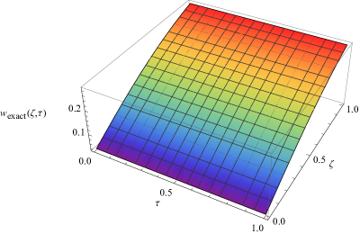
Fig. 1: The 3-D surface solution of (a) $w_{exact}(\zeta,\tau);$ (b) $w_{RKHSM}(\zeta,\tau)$ obtained for the considered example when $\textit{n}=12,\ \alpha=0.5.$

Fig. 2: The 3-D surface solution of (a) $w_{exact}(\zeta,\tau);$ (b) $w_{RKHSM}(\zeta,\tau)$ obtained for the considered example when $\textit{n}=12,~{}\alpha=0.75.$

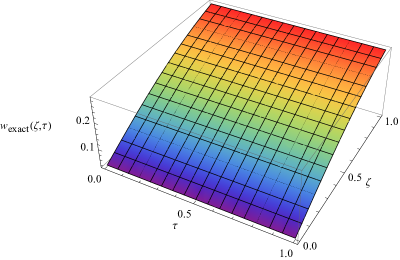
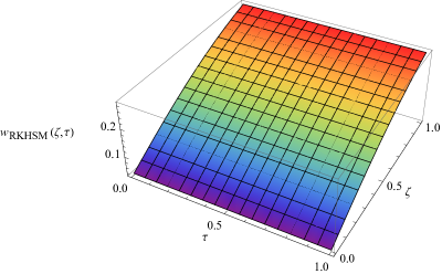
Fig. 3: The 3-D surface solution of (a) $w_{exact}(\zeta,\tau);$ (b) $w_{RKHSM}(\zeta,\tau)$ obtained for the considered example when $\textit{n}=12,~{}\alpha=0.85.$

Fig. 4: The 3-D surface solution of (a) $w_{exact}(\zeta,\tau);$ (b) $w_{RKHSM}(\zeta,\tau)$ obtained for the considered example when $\textit{n}=12,~{}\alpha=0.95.$

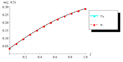
Fig. 5: The 2-D comparison between $w_{exact}(\zeta,\tau)$ and $w_{RKHSM}(\zeta,\tau)$ when $\textit{n}=12,~{}\alpha=0.5.$

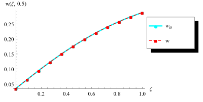
Fig. 6: The 2-D comparison between $w_{exact}(\zeta,\tau)$ and $w_{RKHSM}(\zeta,\tau)$ when $\textit{n}=12,~{}\alpha=0.75.$

Fig. 7: The 2-D comparison between $w_{exact}(\zeta,\tau)$ and $w_{RKHSM}(\zeta,\tau)$ when $\textit{n}=12,~{}\alpha=0.85.$

Fig. 8: The 2-D comparison between $w_{exact}(\zeta,\tau)$ and $w_{RKHSM}(\zeta,\tau)$ when $\textit{n}=12,~{}\alpha=0.95.$

7 Conclusion

The present study implements the RKHSM to solve the time-fractional KSE by introducing some special Hilbert spaces with inner products and the kernel functions. The obtained results are in the form of uniformly convergent series, and the used operator is a bounded linear operator. Error estimation of the approximate solution and convergence analysis are verified with lemma and theorems. The physical interpretation of this method is presented through two-dimensional and three-dimensional graphs. The numerical outputs show that the RKHSM is highly accurate and useful for providing exact and approximate solutions. This present method can be used to study many other high-dimensional FPDEs that abundantly contribute to engineering, applied science, and other fields of science.

8 Acknowledgements

The first author would like to express her gratitude to the “University Grants Commision (UGC),” NTA Ref. No.:191620213691, for providing funding for this work.

References

• [1] Kudryashov, N.A. and Sinelshchikov, D.I., 2010, โ€œNonlinear waves in bubbly liquids with consideration for viscosity and heat transfer,โ€ Physics Letters A, 374(19-20), pp.2011-2016.
• [2] Saha Ray, S. and Singh, S., 2017, โ€œNew exact solutions for the Wick-type stochastic Kudryashovโ€“Sinelshchikov equation,โ€ Communications in Theoretical Physics, 67(2), p.197.
• [3] Gupta, A.K. and Saha Ray, S., 2017, โ€œOn the solitary wave solution of fractional Kudryashovโ€“Sinelshchikov equation describing nonlinear wave processes in a liquid containing gas bubbles,โ€ Applied Mathematics and Computation, 298, pp.1-12.
• [4] Saha Ray, S. and Sahoo, S., 2018, Generalized fractional order differential equations arising in physical models, CRC press.
• [5] Saha Ray, S., 2021, โ€œA new approach by twoโ€dimensional wavelets operational matrix method for solving variableโ€order fractional partial integroโ€differential equations,โ€ Numerical Methods for Partial Differential Equations, 37(1), pp.341-359.
• [6] Saha Ray, S., and Sahoo, S., 2016, โ€œTwo Reliable Efficient Methods for Solving Time Fractional Coupled Klein-Gordon-Schrodinger Equations,โ€ Applied Mathematics and Information Sciences, 10(5), pp.1799-1810.
• [7] Feng, Y.L., Shan, W.R., Sun, W.R., Zhong, H. and Tian, B., 2014, โ€œBifurcation analysis and solutions of a three-dimensional Kudryashovโ€“Sinelshchikov equation in the bubbly liquid,โ€ Communications in Nonlinear Science and Numerical Simulation, 19(4), pp.880-886.
• [8] Yang, H., Liu, W., Yang, B. and He, B., 2015, โ€œLie symmetry analysis and exact explicit solutions of three-dimensional Kudryashovโ€“Sinelshchikov equation,โ€ Communications in Nonlinear Science and Numerical Simulation, 27(1-3), pp.271-280.
• [9] He, Y., Li, S. and Long, Y., 2014, โ€œA improved Fโ€expansion method and its application to Kudryashovโ€“Sinelshchikov equation,โ€ Mathematical Methods in the Applied Sciences, 37(12), pp.1717-1722.
• [10] He, Y., Li, S. and Long, Y., 2013, โ€œExact Solutions of the Kudryashov-Sinelshchikov Equation Using the Multiple-Expansion Method,โ€ Mathematical Problems in Engineering, 2013.
• [11] Inc, M., Akgรผl, A. and Kiliรงman, A., 2012, โ€œExplicit solution of telegraph equation based on reproducing kernel method,โ€ Journal of Function Spaces and Applications, 2012.
• [12] Boutarfa, B., Akgรผl, A. and Inc, M., 2017, โ€œNew approach for the Fornbergโ€“Whitham type equations,โ€ Journal of Computational and Applied Mathematics, 312, pp.13-26.
• [13] Babolian E, Javadi S, Moradi E., โ€œRKM for solving Bratu-type differential equations of fractional order,โ€ Mathematical Methods in the Applied Sciences, 39(6), pp.1548-1557.
• [14] Sakar, M.G., Saldฤฑr, O. and Akgรผl, A., 2019, โ€œA novel technique for fractional Bagleyโ€“Torvik equation,โ€ Proceedings of the National Academy of Sciences, India Section A: Physical Sciences, 89, pp.539-545.
• [15] Geng, F. and Cui, M., 2009. โ€œNew method based on the HPM and RKHSM for solving forced Duffing equations with integral boundary conditions,โ€ Journal of Computational and Applied Mathematics, 233(2), pp.165-172.
• [16] Bushnaq, S., Momani, S. and Zhou, Y., 2013, โ€œA reproducing kernel Hilbert space method for solving integro-differential equations of fractional order,โ€ Journal of Optimization Theory and Applications, 156, pp.96-105.
• [17] Inc, M., Akgรผl, A. and Kฤฑlฤฑรงman, A., 2013, โ€œA new application of the reproducing kernel Hilbert space method to solve MHD Jeffery-Hamel flows problem in nonparallel walls,โ€ In Abstract and Applied Analysis, 2013.
• [18] Sakar, M.G., Saldฤฑr, O. and Erdogan, F., 2018, โ€œAn iterative approximation for time-fractional Cahnโ€“Allen equation with reproducing kernel method,โ€ Computational and Applied Mathematics, 37, pp.5951-5964.