Correcting heading errors in optically pumped magnetometers through microwave interrogation

Abstract

We demonstrate how to measure in-situ for heading errors of optically pumped magnetometers in geomagnetic fields. For this, we implement microwave-driven Rabi oscillations and Ramsey interferometry on hyperfine transitions as two independent methods to detect scalar systematics of free induction decay (FID) signals. We showcase the wide applicability of this technique by operating in the challenging parameter regime of compact vapor cells with imperfect pumping and high buffer gas pressure. In this system, we achieve suppression of large inaccuracies arising from nonlinear Zeeman (NLZ) shifts by up to a factor of 10 to levels below 0.6 nT. In the Ramsey method we accomplish this, even in arbitrary magnetic field directions, by employing a hyper-Ramsey protocol and optical pumping with adiabatic power ramps. For the Rabi technique, this level of accuracy is reached, despite associated drive-dependent shifts, by referencing Rabi frequency measurements to a complete atom-microwave coupling model that incorporates the microwave polarization structure.

Optically pumped magnetometers (OPMs) are state-of-the-art sensors that can reach sensitivities below 1 fT $/\sqrt{\text{Hz}}$ kominis2003subfemtotesla ; budker2007optical ; dang2010ultrahigh ; sheng2013subfemtotesla , enable precise detection of biomagnetic signals bison2003laser ; xia2006magnetoencephalography ; broser2018optically , and push the boundaries for scientific exploration by aiding in searches for permanent electron dipole moments pendlebury1984search ; ayres2021design and dark matter pospelov2013detecting ; afach2021search . Practical use of OPMs in geomagnetic fields such as navigation psiaki1993ground ; canciani2016absolute , geophysics friis2006swarm ; stolle2021special , space dougherty2004cassini ; korth2016miniature ; bennett2021precision , and unexploded ordinance detection billings2004discrimination ; prouty2016real requires addressing systematic errors that depend on the orientation of the sensor with respect to the magnetic field known as heading errors. For the most common OPMs made of alkali atoms the dominant heading error at geomagnetic fields is on the order of 10 nT. This systematic error manifests from unknown strengths of unresolved frequency components in the magnetometer signal arising from nonlinear Zeeman (NLZ) shifts from each of the ground state hyperfine manifolds alexandrov2003recent ; lee2021heading .

Only in regimes of narrow magnetic resonances acosta2006nonlinear and high spin polarization can this heading error be accurately modeled to 0.1 nT lee2021heading . In MEMS vapor cells, these regimes often become unfeasible due to line broadening from atomic collisions and the challenges associated with implementing fast, high-fidelity optical pumping using modest pump powers. Various other approaches have been developed to mitigate heading error including spin locking bao2018suppression ; bao2022all , light polarization modulation oelsner2019sources , double-pass configurations rosenzweig2023heading , double-modulated synchronous pumping seltzer2007synchronous , and leverage of tensor lightshifts jensen2009cancellation , but all these approaches neglect frequency shifts arising from the different Zeeman resonances between the $F=I\pm 1/2$ manifolds and have their own practical challenges. Furthermore, methods that utilize higher-order polarization moments zhang2023heading ; acosta2008production ; yashchuk2003selective are not feasible in compact OPM packages with high buffer gas pressures rushton2023alignment . CPT magnetometry pollinger2018coupled ; liang2014simultaneously holds promise for high scalar accuracy by detecting multiple hyperfine resonances to address NLZ systematics, though sub-nT accuracy in microfabricated cells remains elusive to date.

Sensitive hyperfine spectroscopy in microfabricated cells has been demonstrated with pulsed batori2022mupop and continuous horsley2013imaging ; kiehl2023coherence microwave interrogation. Although both of these domains show promise for accurate magnetic sensing, managing systematic shifts in arbitrary field directions remains an issue. Rabi oscillations, for example, that utilize uninterrupted microwave interrogation, enable self-calibrated vector operation thiele2018self , but are highly sensitive to systematic shifts from off-resonant driving. Conversely, Ramsey interferometry protocols employed for spectroscopy of hyperfine transitions, as implemented in vapor cell atomic clocks batori2022mupop ; affolderbach2018study ; cutler1991frequency , utilize short periods of microwave interrogation to mitigate off-resonant driving, but require linearly polarized microwave sources along a well-defined magnetic field. In this Letter, we solve these microwave interrogation challenges and directly measure the heading error of a microfabricated OPM based on free induction decay (FID) with sub-nT accuracy.

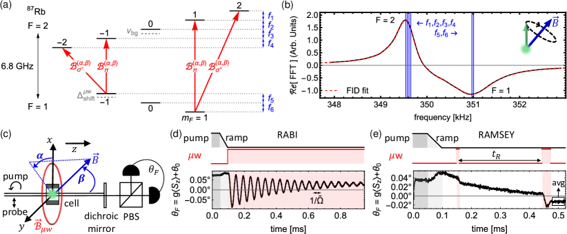
Figure 1: (a) Energy-level diagram showing the four hyperfine transitions used in Rabi and Ramsey frequency spectroscopy to correct FID heading error. Nonlinear Zeeman splittings $f_{i}$ (blue) contribute to the Larmor FID signal. Buffer gas pressure shift $\nu_{\text{bg}}\approx 88$ kHz further shifts the hyperfine manifolds. (b) FID signal measured at $\beta=106\degree$ in the regime of low-polarization pumping that contains both $F=1$ and $F=2$ precession frequencies. Heading errors arise due to the uncertainty in the amplitudes and relative phases of the nonlinear Zeeman frequencies (blue lines). (c) Magnetometer apparatus to measure magnetic fields with direction specified by azimuthal ($\alpha$) and polar ($\beta$) angles. (d,e) Rabi and Ramsey pulse sequences evaluated at $\beta=35\degree$ and plotted with a moving average of 10 data points, respectively.

Specifically, we use Rabi and Ramsey frequency spectroscopy that respectively use continuous and pulsed microwave interrogation to detect Zeeman shifts between four hyperfine transitions of ⁸⁷Rb shown in Fig. 1a. Both techniques can be applied at the same set of vapor cell parameters used for sensitive FID measurements. In Rabi frequency spectroscopy, an atom-microwave Hamiltonian that utilizes calibrated microwave polarization ellipse (MPE) parameters thiele2018self accurately models Rabi oscillation frequencies despite frequency shifts due to off-resonant driving. In contrast, Ramsey frequency spectroscopy does not directly model atom-microwave coupling, but instead mitigates systematics by varying both the Ramsey time $t_{R}$ and microwave detuning within a $\pi/2-t_{R}-3\pi/2$ hyper-Ramsey sequence yudin2010hyper . To prevent signal degradation in arbitrary magnetic field directions, both techniques employ adiabatic power ramps during optical pumping to suppress Larmor precession. We compare these two methods to FID measurements over a range of DC magnetic field directions at 50 $\mu$T. We find the Rabi and Ramsey techniques, despite their distinct concepts, both measure the FID heading error with agreement to within 0.6 nT. From theoretical simulations, we find that the fundamental accuracy of both approaches is within 0.4 nT due to spin-exchange frequency shifts micalizio2006spin ; appelt1998theory .

The magnetometer apparatus [Fig. 1c] consists of a $3\times 3\times 2$ mm³ microfabricated vapor cell with a single optical axis, heated to near 100$\degree$C, and filled with 180 Torr of N₂ buffer gas. At this buffer gas pressure, Rb-N₂ collisions broaden the optical D1 and D2 transitions to 5.6 GHz. The vapor cell is contained within a rectangular microwave cavity that is the source for driving hyperfine transitions and is detailed in kiehl2023coherence . A 3D coil system defines an orthogonal reference frame $(x,y,z)$, where a calibration corrects for non-orthogonal misalignments between the coil pairs (Supplementary Material suppMat ). This coil system generates a programmable 50 $\mu$T magnetic field $\vec{B}$, defined by azimuthal and polar angles $\alpha$ and $\beta$. Along the single optical axis propagates a 795 nm elliptically polarized pump beam, tuned within a few GHz of the D₁ line, and a 1 mW probe beam blue-detuned by 170 GHz from the 780 nm $D_{2}$ line. A polarimeter detects the Faraday rotation $\theta_{F}=g\langle S_{z}\rangle+\theta_{0}$ of the probe beam expressed in terms of the macroscopic z-component of the electron spin, a coupling coefficient $g$, and an offset $\theta_{0}$ seltzer2008developments .

For comparative demonstration, we study FID spin-precession signals with low atomic spin polarization where no accurate physical models for heading errors exist. To initiate FID measurements in this low polarization regime, a 100 $\mu$s pulse of pump light at 400 mW polarizes atomic spins along the pump beam. In this low spin polarization regime, the FID spectrum [Fig. 1b] consists of both, $F=1$ and $F=2$ Zeeman resonances that are separated at 50 $\mu$T by 1.4 kHz. The NLZ effect splits these resonances into frequency components $\{f_{1},...,f_{6}\}$ separated by 36 Hz. We model the FID spectrum as two resonances $f_{L,\pm}(B)\approx\mu_{B}(g_{s}-g_{i}\pm 4g_{i})B/4h$ that are the mean Zeeman splitting across the magnetic sublevels for the $F=I\pm 1/2$ manifolds, where $I=3/2$ is the nuclear spin, $g_{s}$ and $g_{i}$ are the electronic and nuclear Landé g-factors, $h$ is Planck’s constant, $\mu_{B}$ is the Bohr magneton, and $B$ is the magnetic field strength. The real component of the FID signal’s Fourier transform in this model is given by

$$\mathcal{R}e[\text{FFT}]=\sum_{j=\pm}a_{j}\frac{\text{cos}[\phi_{j}]-\text{sin}[\phi_{j}](f-f_{L,j})}{(f-f_{L,j})^{2}+w_{j}^{2}/4}$$ (1)

where $\phi_{\pm}=2\pi f_{L,\pm}t_{0}\pm\phi/2$ are phase shifts due to a starting time offset $t_{0}$ with $\phi$ being a relative phase between the $I\pm 1/2$ resonances respectively. Here the strength and broadening of this signal is given by amplitudes $a_{\pm}$ and linewidths $w_{\pm}\approx 1$ kHz. Based on the initial atomic state and the direction of $\vec{B}$, heading error arises in this model from the unresolved NLZ frequency components that bias the observed resonances from $f_{L,\pm}$.

Rabi and Ramsey frequency spectroscopy avoid these heading errors by detecting Zeeman shifts between resolved hyperfine transitions highlighted in Fig. 1a. To make these measurements in arbitrary magnetic field directions, we first optically pump the atomic ensemble for 50 $\mu$s at 100 mW and then linearly ramp off the pump power over the next 50 $\mu$s [Fig. 1(d,e)]. This linear ramp suppresses Larmor precession by adiabatically orienting the atomic spins along the magnetic field $\vec{B}$ suppMat .

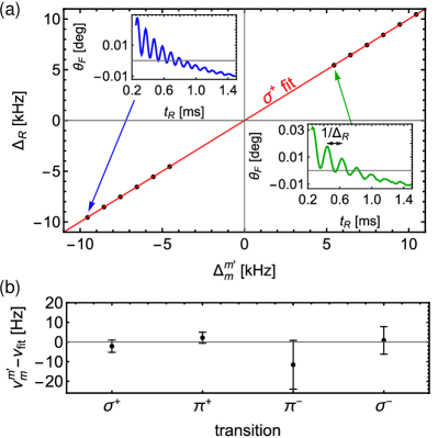
Figure 2: Ramsey frequency spectroscopy at $\beta=35\degree$. (a) Ramsey frequency vs microwave detuning for the $\sigma^{+}$ transition. Insets show measured Ramsey fringes as a function of the Ramsey time $t_{R}$. A linear fit (red) extracts the microwave resonance. (b) Residuals of fitting Eq. (2) to the measured hyperfine resonances. Error bars show 68% confidence interval.

Ramsey frequency spectroscopy utilizes pulsed microwave interrogation to accurately measure any hyperfine resonance $\nu_{m}^{m^{\prime}}\approx 6.8$ GHz between sublevels $\ket{1,m}$ and $\ket{2,m^{\prime}}$ without exact knowledge of off-resonant driving. This is achieved through a $\pi/2-t_{R}-3\pi/2$ hyper-Ramsey pulse sequence yudin2010hyper with $t_{\pi/2}=4/\tilde{\Omega}_{m}^{m^{\prime}}\approx 10$ $\mu$s [Fig. 1e]. Satisfying this particular $t_{\pi/2}$ required manual adjustments to the microwave power at each magnetic field direction and hyperfine transition such that the generalized Rabi frequency satisfied $\tilde{\Omega}_{m}^{m^{\prime}}\approx 25$ kHz. Importantly after each pulse sequence, we average the resulting Faraday signal for $50$ $\mu$s to filter out residual 350 kHz Larmor precession [Fig. 1e].

By varying the Ramsey free evolution time $t_{R}$ between 0.2 ms and 1.43 ms at 10 $\mu$s spacing, we measure Ramsey fringes at each microwave detuning as shown in the insets of Fig. 2a. We fit these Ramsey fringes in the time-domain using an exponentially decaying sinusoid suppMat and force the fringe frequencies $\Delta_{R}$ to be either positive or negative according to the sign of the microwave detuning $\Delta_{m}^{m^{\prime}}=\nu_{\mu\text{w}}-\nu_{m}^{m^{\prime}}$. Without influence from systematic shifts, $\Delta_{R}=\Delta_{m}^{m^{\prime}}$. We choose 6 microwave detunings $\Delta_{m}^{m^{\prime}}\in[5,10]$ kHz below and above each transition resonance as shown for the $\sigma^{+}$ transition in Fig. 2a. All of these measurements are taken in random order to mitigate systematics from time-dependent drifts in the microwave field. By linear fitting $\Delta_{R}$ as a function of the microwave frequency $\nu_{\mu\text{w}}$, the x-intercept measures $\nu_{m}^{m^{\prime}}$. The magnetic field $B$ and the pressure shift arising from N₂ buffer gas collisions $\nu_{\text{bg}}\approx 88$ kHz are obtained by fitting [Fig. 2b] $\nu_{m}^{m^{\prime}}$ measurements to

$$\frac{h\nu_{m}^{m^{\prime}}}{\Delta E}=\frac{m^{\prime}-m}{g_{s}/g_{i}-1}x+\frac{1}{2}\sum_{M=m,m^{\prime}}\sqrt{1+\frac{4Mx}{2I+1}+x^{2}}$$ (2)

where $x=(g_{s}-g_{i})\mu_{B}B/\Delta E$ and $\Delta E=(A+h\nu_{\text{bg}}/2)(I+1/2)$ is the hyperfine splitting expressed in terms of the magnetic dipole hyperfine constant $A$.

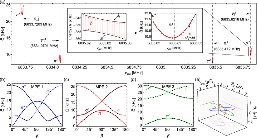
Figure 3: Rabi frequency spectroscopy and microwave polarization ellipse calibration (a) Generalized Rabi frequency measurements at $\beta=35\degree$, driven by MPE 2, with a center microwave frequencies $\overline{\nu}_{m}^{m^{\prime}}$ (dashed lines). The inset shows a fit of the $\sigma^{+}$ transition using the eigenstates of $H$ defined in Eq. (3). (b-d) Polar angle dependence of Rabi-frequency measurements for the $\sigma^{+},\pi^{+}$, and $\sigma^{-}$ hyperfine transitions. Solid lines show fits to calibrate the polarization ellipses. (e) Fitted polarization ellipses.

Alternatively, Rabi frequency spectroscopy [Fig. 3a] measures these hyperfine resonances from the detuning $\Delta_{m}^{m^{\prime}}$ dependence of generalized Rabi frequencies $(\tilde{\Omega}_{m}^{m^{\prime}})^{2}\approx(\Delta_{m}^{m^{\prime}})^{2}+|\Omega_{m}^{m^{\prime}}|^{2}$ that are fitted from Rabi oscillations using an exponentially decaying sinusoid suppMat . Unlike Ramsey frequency spectroscopy, this approach demands precise modeling of atom-microwave coupling to accommodate for frequency shifts from off-resonant driving. At a microwave frequency $\nu_{\mu\text{w}}$, the atom-microwave coupling is quantified by the following Hamiltonian

$$\begin{split}H=&\mathcal{M}\big{[}(A+h\frac{\nu_{\text{bg}}}{2})\mathbf{S}\cdot\mathbf{I}+\mu_{B}(g_{s}S_{z}+g_{i}I_{z})B\big{]}\mathcal{M}^{\dagger}-\\ &I_{2}h\nu_{\mu\text{w}}+\sum_{|m-m^{\prime}|\leq 1}\frac{h}{2}\Big{[}\ket{\overline{2,m^{\prime}}}\Omega_{m}^{m^{\prime}}\bra{\overline{1,m}}+\text{h.c.}\Big{]}\end{split}$$ (3)

where $I_{2}$ is the $F=2$ identity operator. In order to preserve NLZ effects during the rotating-wave approximation (RWA), we work in a modified hyperfine basis $\ket{\overline{F,m}}=\mathcal{M}\ket{F,m}$ with $\mathcal{M}$ being defined as the operator that diagonalizes the hyperfine and Zeeman terms in the first line of Eq. (3). An analytical expression for $\mathcal{M}$ is shown in the Supplementary Material suppMat . The Rabi frequency is given by

$$\Omega_{m}^{m^{\prime}}=\mu_{m}^{m^{\prime}}\mathcal{B}^{(\alpha,\beta)}_{k}/h$$ (4)

where $\mu_{m}^{m^{\prime}}$ denotes the corresponding magnetic transition dipole moment suppMat and $k=\pm,\pi$ denotes the polarization of the hyperfine transition. The spherical microwave components [Fig. 1a]

$$\mathcal{B}^{(\alpha,\beta)}_{k}=R_{z}(\alpha)R_{y}(\beta)\{\mathcal{B}_{x}e^{-i\phi_{x}},\mathcal{B}_{y}e^{-i\phi_{y}},\mathcal{B}_{z}\}\cdot\hat{\epsilon}_{k}$$ (5)

are defined in terms of an MPE phasor that is projected onto the spherical basis $\epsilon_{\pm}=\{\frac{1}{\sqrt{2}},\mp\frac{i}{\sqrt{2}},0\}$ and $\epsilon_{\pi}=\{0,0,1\}$. This MPE phasor contains the three microwave amplitudes ($\mathcal{B}_{x},\mathcal{B}_{y},\mathcal{B}_{z}$) and two relative phases ($\phi_{x},\phi_{y}$) that fully define any MPE thiele2018self . To account for different magnetic field directions $(\alpha,\beta)$ in the lab frame, we assume, without loss of generality, that the magnetic field $\vec{B}$ points along $z$ and rotate the MPE phasor using 3D rotation operators $R_{y,z}$.

The atom-microwave Hamiltonian defined in Eq. (3) accounts for systematic shifts in the Rabi oscillations from off-resonant driving through the expression $h\tilde{\Omega}_{m}^{m^{\prime}}=\lambda_{j}-\lambda_{i}$, where eigenvalues $\lambda_{j}$ and $\lambda_{i}$ of $H$ correspond to the pair of dressed states coupled by the microwave field. With this model, the magnetic field strength $B$ and the pressure shift $\nu_{\text{bg}}$ are fitted from generalized Rabi frequencies $\tilde{\Omega}_{m}^{m^{\prime}}$, driven at 25 microwave detunings $\Delta_{m}^{m^{\prime}}$ spaced by 800 Hz, with center frequency $\overline{\nu}_{m}^{m^{\prime}}$ that is near-resonant with the hyperfine transitions $\nu_{m}^{m^{\prime}}$ [Fig. 2a]. For weak coupling ($\Omega_{m}^{m^{\prime}}\ll f_{L,\pm}$), where it’s valid to approximate $\Omega_{m}^{m^{\prime}}=|\Omega_{m}^{m^{\prime}}|$ in $H$, and when the MPE shows no dependence on $\nu_{\mu\text{w}}$, all Rabi rates in $H$ are accurately known from these measurements using the dipole moments $\mu_{m}^{m^{\prime}}$. This work operates close to the weak atom-microwave coupling limit, but due to the lineshape of the microwave cavity modes, there is a different MPE at each hyperfine transition frequency. We account for this by performing four separate MPE calibrations at each microwave frequency $\overline{\nu}_{m}^{m^{\prime}}$. While the Rabi rates $|\Omega_{m}^{m^{\prime}}|$ evaluated about $\overline{\nu}_{m}^{m^{\prime}}$, the pressure shift $\nu_{\text{bg}}$, and the magnetic field strength $B$ are fitting parameters, the corresponding arguments Arg($\Omega_{m}^{m^{\prime}}$) and all other complex Rabi rates in Eq. (3) at each $\nu_{\mu\text{w}}$ are calculated from these MPE calibrations using Eq. (4) with the field direction $(\alpha,\beta)$ known from the coil system. Possible systematic errors arising from additional MPE $\nu_{\mu\text{w}}$-dependence about each $\overline{\nu}_{m}^{m^{\prime}}$ are estimated in the Supplementary Material suppMat .

We perform MPE calibrations by measuring generalized Rabi frequencies $\tilde{\Omega}_{m}^{m^{\prime}}$ at each $\overline{\nu}_{m}^{m^{\prime}}$ and at 14 different magnetic field directions by varying $\beta$ and setting $\alpha=0$. From these 14 measurements, we fit the 5 MPE parameters ($\mathcal{B}_{x},\mathcal{B}_{y},\mathcal{B}_{z},\phi_{x},\phi_{y}$) for each $\overline{\nu}_{m}^{m^{\prime}}$ using the eigenvalues of $H$ [Fig. 2(b-d)]. During these calibrations we leave $\nu_{\text{bg}}$ as a fitting parameter and use FID measurements to estimate $B$. FID systematic errors are not a concern for these calibrations since $\tilde{\Omega}_{m}^{m^{\prime}}$ depends on $\Delta_{m}^{m^{\prime}}$ in second-order near the transition resonance.

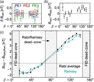
Figure 4: Comparing FID, Rabi, and Ramsey scalar measurements over different magnetic field directions. Error bars show 68% confidence intervals. (a) Differences between Rabi scalar measurements for each MPE with respect to the average scalar across all MPEs. (b) Differences between Ramsey and Rabi scalar. (c) Differences between FID measurements with Ramsey (cyan) and Rabi (black) scalar measurements.

The FID measurements differ from the Rabi and Ramsey scalar measurements by up to 5 nT over the 14 $\vec{B}$ directions [Fig. 4c]. Heading errors qualitatively similar to Fig. 4c are predicted from simulations in the Supplementary Material suppMat using experimental parameters. Despite different systematic errors from off-resonant driving, the Rabi scalar measurements across different MPEs are consistent to within $0.5$ nT [Fig. 4a]. For these Rabi measurements in Fig. 4, we only use $\sigma^{\pm}$ transitions since we found that the $\pi^{\pm}$ transitions are more sensitive to systematic shifts causing nT-scale discrepancies between different MPE evaluations. This observation is consistent with theoretical simulations that account for MPE $\nu_{\mu\text{w}}$-dependence, spin-exchange frequency shifts micalizio2006spin ; appelt1998theory , as well as lineshape distortions from atomic collisions that are detailed in the Supplementary Material suppMat . From these theoretical simulations we estimate scalar errors to be contained within 0.6 nT for the Rabi and Ramsey methods. These simulations show that a large portion of errors ($<0.4$ nT) arise due to frequency shifts from spin-exchange collisions. These estimates, along with drifts of the optical-pumping parameters, are consistent with the measured differences, bounded by 0.6 nT, between the Ramsey and Rabi measurements [Fig. 4b].

These results demonstrate how tailored atom-microwave interrogation through Rabi and Ramsey spectroscopy reduces OPM heading error to the sub-nT regime at geomagnetic fields and other challenging domains such as the high buffer gas pressure environments utilized in microfabricated vapor cells and regimes of weak optical pumping. Demonstration of the Rabi technique as an accurate measure via the scalar comparison establishes a solid foundation to use Rabi for accurate vector magnetometry kiehlVector .

- (1) I. K. Kominis, T. W. Kornack, J. C. Allred, and M. V. Romalis, Nature, 422, 596-599 (2003).
- (2) D. Budker and M. Romalis, Nat. Phys. 3, 227 (2007)
- (3) H. B. Dang, A. C. Maloof, M. V. Romalis, Appl. Phys. Lett. 97, 151110 (2010).
- (4) D. Sheng, S. Li, N. Dural, and M. V. Romalis, Phys. Rev. Lett., 110, 160802 (2013).
- (5) G. Bison, R. Wynands, and A. Weis, Appl. Phys. B 76, 325–328 (2003)
- (6) H. Xia, A. B.-A. Baranga, D. Hoffman, M. V. Romalis, Appl. Phys. Lett. 97, 151110 (2010).
- (7) P. J. Broser, S. Knappe, D.-S. Kajal, N. Noury, O. Alem, V. Shah, and C. Braun, IEEE Trans. Neural Syst. Rehabil. Eng., 26, 2226–2230 (2018).
- (8) J. M. Pendlebury et al., Phys. Lett. 13, 327-330 (1984)
- (9) N. J. Ayres et al., Eur. Phys. J. C, 81, 512 (2021).
- (10) M. Pospelov, S. Pustelny, M. P. Ledbetter, D. F. Jackson Kimball, W. Gawlik, and D. Budker, Phys. Rev. Lett., 110, 021803 (2013).
- (11) S. Afach et al., Nat. Phys., 17, 1396–1401 (2021).
- (12) M. L. Psiaki, L. Huang, and S. M. Fox, J. Guid. Control Dyn., 16, 206-214 (1993).
- (13) A. Canciani and J. Raquet, Navig. J. Inst. Navig., 63, 111-126 (2016).
- (14) E. Friis-Christensen and H. Lühr, G. Hulot, EPS, 58, 351–358 (2006).
- (15) C. Stolle, N. Olsen, B. Anderson, E. Doornbos, and A. Kuvshinov, EPS, 73, 83 (2021).
- (16) M. K. Dougherty et al., Space Sci. Rev., 114, 331–383 (2004).
- (17) H. Korth, K. Strohbehn, F. Tejada, A. G. Andreou, J. Kitching, S. Knappe, S. J. Lehtonen, S. M. London, and M. Kafel, J. Geophys. Res.: Space Phys., 121, 7870-7880 (2016).
- (18) J. S. Bennett, B. E. Vyhnalek, H. Greenall, E. M. Bridge, F. Gotardo, S. Forstner, G. I. Harris, F. A. Miranda, and W. P. Bowen, Sensors, 21, 5568 (2021).
- (19) S. D. Billins, IEEE Trans. Geosci. Remote Sens., 42, 1241–1251 (2004).
- (20) M. Prouty, Real-Time Hand-Held Magnetometer Array, Geometrics, Inc., (2016).
- (21) E. B. Alexandrov, Recent progress in optically pumped magnetometers, Phys. Scr., 2003(T105), 27 (2003).
- (22) W. Lee, V. G. Lucivero, M. V. Romalis, M. E. Limes, E. L. Foley, and T. W. Kornack, Phys. Rev. A, 103, 063103 (2021).
- (23) V. Acosta, M. P. Ledbetter, S. M. Rochester, D. Budker, D. F. Jackson Kimball, D. C. Hovde, W. Gawlik, S. Pustelny, J. Zachorowski, and V. V. Yashchuk, Phys. Rev. A, 73, 053404 (2006).
- (24) G. Bao, A. Wickenbrock, S. Rochester, W. Zhang, and D. Budker, Phys. Rev. Lett., 120, 033202 (2018).
- (25) G. Bao, D. Kanta, D. Antypas, S. Rochester, K. Jensen, W. Zhang, A. Wickenbrock, and D. Budker, Phys. Rev. A, 105, 043109 (2022).
- (26) G. Oelsner, V. Schultze, R. IJsselsteijn, F. Wittkämper, and R. Stolz, Phys. Rev. A, 99, 013420 (2019).
- (27) Y. Rosenzweig, D. Tokar, I. Shcerback, M. Givon, and R. Folman, arXiv:2307.13982.
- (28) S. J. Seltzer, P. J. Meares, and M. V. Romalis, Phys. Rev. A, 75, 051407(R) (2007).
- (29) K. Jensen, V. M. Acosta, J. M. Higbie, M. P. Ledbetter, S. M. Rochester, and D. Budker, Phys. Rev. A, 79, 023406 (2009).
- (30) Rui Zhang, Dimitra Kanta, Arne Wickenbrock, Hong Guo, and Dmitry Budker, Phys. Rev. Lett., 130, 153601 (2023).
- (31) V. M. Acosta et al., Opt. Express, 16, 11423–11430 (2008).
- (32) V. V. Yashchuk, D. Budker, W. Gawlik, D. F. Kimball, Yu. P. Malakyan, and S. M. Rochester, Phys. Rev. Lett., 90, 253001 (2003).
- (33) L.M. Rushton, L. Elson, A. Meraki, and K. Jensen, Phys. Rev. Appl., 19, 064047 (2023).
- (34) A. Pollinger et al. 2018 Meas. Sci. Technol. 29 095103
- (35) S.-Q. Liang, G.-Q. Yang, Y.-F. Xu, Q. Lin, Z.-H. Liu, and Z.-X. Chen, Opt. Express, 22, 6837-6843 (2014).
- (36) E. Batori, C. Affolderbach, M. Pellaton, F. Gruet, M. Violetti, Y. Su, A. K. Skrivervik, and G. Mileti, Phys. Rev. Appl., 18, 054039 (2022).
- (37) C. Kiehl, D. Wagner, T.-W. Hsu, S. Knappe, C. A. Regal, and T. Thiele, Phys. Rev. Research, 5, L012002 (2023).
- (38) A. Horsley, G.-X. Du, M. Pellaton, C. Affolderbach, G. Mileti, and P. Treutlein, Phys. Rev. A, 88, 063407 (2013).
- (39) T. Thiele, Y. Lin, M. O. Brown, and C. A. Regal, Phys. Rev. Lett., 121, 153202 (2018).
- (40) C. Affolderbach, W. Moreno, A. E. Ivanov, T. Debogovic, M. Pellaton, A. K. Skrivervik, E. de Rijk, and G. Mileti, Appl. Phys. Lett., 112, 113502 (2018).
- (41) L. S. Cutler, C. A. Flory, R. P. Giffard, A. De Marchi, J. Appl. Phys., 69, 2780–2792 (1991).
- (42) V. I. Yudin, A. V. Taichenachev, C. W. Oates, Z. W. Barber, N. D. Lemke, A. D. Ludlow, U. Sterr, Ch. Lisdat, and F. Riehle, Phys. Rev. A, 82, 011804(R) (2010).
- (43) S. Micalizio, A. Godone, F. Levi, and J. Vanier, Phys. Rev. A 73, 033414 (2006).
- (44) S. Appelt, A. B. Baranga, C. J. Erickson, M. V. Romalis, A. R. Young, and W. Happer, Phys. Rev. A 58, 1412 (1998).
- (45) See Supplemental Material for additional information on the coil system calibration, data collection, Rabi frequency spectroscopy analysis, and simulations of adiabatic optical pumping, FID heading error, and systematic errors in Ramsey and Rabi frequency spectroscopy, which includes Refs. [46-55].
- (46) S. J. Seltzer, PhD, Princeton University, (2008).
- (47) Y. Horowicz, O. Katz, O. Raz, and O. Firstenberg, Proc. Natl. Acad. Sci. U.S.A 118 (2021)
- (48) W. Happer, Y. Y. Jau, T. Walker, Optically Pumped Atoms (John Wiley & Sons, 2010)
- (49) D. A. Steck, Rubidium 87 D Line Data, available online at http://steck.us/alkalidata (revision 2.2.2, 9 July 2021)
- (50) A. Pouliot, G. Carlse, H. C. Beica, T. Vacheresse, A. Kumarakrishnan, U. Shim, S. B. Cahn, A. Turlapov, and T. Sleator, Phys. Rev. A. 103, 023112 (2021).
- (51) E. S. Thiele Hrycyshyn and L. Krause, Can. J. Phys., 48 (1970).
- (52) M. E. Wagshul and T. E. Chupp, Phys. Rev. A 40, 4447 (1989).
- (53) D. K. Walter, W. M. Griffith, and W. Happer, Phys. Rev. Lett. 88, 093004 (2002).
- (54) O. Katz, and O. Firstenberg, Commun. Phys. 2, 58 (2019).
- (55) J. Vanier and C. Audoin, The quantum physics of atomic frequency standards, Vol 1 (Bristol: A. Hilger, 1989).
- (56) C. Kiehl, T. S. Menon, S. Knappe, T. Thiele, and C. A. Regal (unpublished).