Abstract

We study the federated pure exploration problem of multi-armed bandits and linear bandits, where $M$ agents cooperatively identify the best arm via communicating with the central server. To enhance the robustness against latency and unavailability of agents that are common in practice, we propose the first federated asynchronous multi-armed bandit and linear bandit algorithms for pure exploration with fixed confidence. Our theoretical analysis shows the proposed algorithms achieve near-optimal sample complexities and efficient communication costs in a fully asynchronous environment. Moreover, experimental results based on synthetic and real-world data empirically elucidate the effectiveness and communication cost-efficiency of the proposed algorithms.

1 INTRODUCTION

Multi-Armed Bandits (MAB) [Auer et al., 2002, Lattimore and Szepesvári, 2020] is a classic sequential decision-making model that is characterized by the exploration-exploitation tradeoff. Pure exploration [Even-Dar et al., 2006, Soare et al., 2014, Bubeck et al., 2009], also known as best arm identification, is an important variant of the MAB problems where the objective is to identify the arm with the maximum expected reward. While most existing bandit solutions are designed under a centralized setting (i.e., data is readily available at a central server), there is increasing interest in federated bandits in terms of regret minimization [Wang et al., 2019, Li et al., 2022, He et al., 2022] and pure exploration [Hillel et al., 2013, Tao et al., 2019, Du et al., 2021] due to the increasing application scale and public concerns about privacy. Specifically, pure exploration for federated bandits considers $M$ agents identifying the best arm collaboratively with limited communication bandwidth, while keeping each agent’s raw data local. In federated bandits, the major challenge is the conflict between the need for timely data/model aggregation for low sample complexity and the need for communication efficiency with decentralized agents. Balancing model updates and communication is vital to efficiently solve the problem.

Prior works on distributed/federated pure exploration [Hillel et al., 2013, Tao et al., 2019, R’eda et al., 2022, Du et al., 2021] all focused on synchronous communication protocols, where all agents simultaneously participate in each communication round to exchange their latest observations with a central server (federated setting) or other agents (distributed setting). However, the synchronous setting cannot enjoy efficient communication in real-world applications due to 1) some agents may not interact with the environment in certain rounds and 2) the communication in a global synchronous setting needs to wait until the slowest agent responds to the server, which incurs a significant latency especially when the number of the agents is large and the communication is unstable.

To address the aforementioned challenges of model updates and communication, we study the asynchronous communication for federated pure exploration problem in this paper. We consider both stochastic multi-armed bandit and linear bandit settings. To reduce communication costs, we propose novel asynchronous event-triggered communication protocols where each agent sends local updates to and receives aggregated updates from the server independently from other agents, i.e., global synchronization is no longer needed. This improves the robustness against possible delays and unavailability of agents. Event-triggered communication only happens when the agent has a significant amount of new observations, which reduces communication costs while maintaining low sample complexity.

With the new communication protocols, we proposed two asynchronous federated pure exploration algorithms, Federated Asynchronous MAB Pure Exploration (FAMABPE) and Federated Asynchronous Linear Pure Exploration (FALinPE) for MAB and linear bandits, respectively. We theoretically analyzed that these algorithms can return $(\epsilon,\delta)$-best arm with an efficient communication cost, efficient switching cost and near-optimal sample complexity, where the returned arm is $\epsilon$ close to the best arm with probability at least $1-\delta$, known as fixed confidence setting [Gabillon et al., 2012, Soare et al., 2014, Xu et al., 2017]. We also provide the first $\Omega(M)$ communication cost lower bound for the asynchronous MAB pure exploration problem. Together with the communication cost upper bound $\tilde{O}(M^{3/2}K)$ of FAMABPE and the communication cost lower bound $\Omega(M)$, it suggests there is only a $M^{1/2}K$ gap between the upper bound and lower bound. Moreover, we empirically validated the theoretical results based on synthetic data and real-world data. Experimental results showed that our event-triggered communication strategy can achieve efficient communication cost, and would only moderately affect the sample complexity compared with the synchronous baselines.

2 RELATED WORK

Pure exploration.

The pure exploration problem in the single agent setting was first investigated by Mannor and Tsitsiklis [2004], Even-Dar et al. [2006], Bubeck et al. [2009], Gabillon et al. [2011, 2012], Jamieson et al. [2013], Garivier and Kaufmann [2016], Chen et al. [2016], which focused on the MAB. Then, Soare et al. [2014], Xu et al. [2017], Tao et al. [2018], Kazerouni and Wein [2019], Fiez et al. [2019], Degenne et al. [2020], Jedra and Proutière [2020] extended their results to the linear bandits. Moreover, Scarlett et al. [2017], Vakili et al. [2021], Zhu et al. [2021a], Camilleri et al. [2021] further extended the previous results to the kernelized bandits. However, these algorithms suffer from long learning process and would lose their effectiveness when the sample budget of the single agent is limited. Therefore, in this paper, we consider the setting in which agents collaboratively solve the pure exploration problem.

Distributed/federated pure exploration.

The pure exploration problem in distributed/federated bandits has received much interest in recent studies. For instance, Hillel et al. [2013], Tao et al. [2019], Karpov et al. [2020], Mitra et al. [2021], R’eda et al. [2022], Chen et al. [2022], Reddy et al. [2022] studied the MAB in a synchronous environment. Besides, Du et al. [2021] studied the kernelized bandits in a synchronous environment. These works focused on the synchronous setting and many of them utilized experimental design to derive the exploration sequence. However, this category of algorithms can hardly work in an asynchronous environment due to they require 1. the global synchronous communication round, 2. the active agent in every round should be known to the server in advance and 3. the time index $t$ should be known to the server and agents. In this paper, we alleviate these requirements and propose the first truly asynchronous algorithms for federated pure exploration with fixed confidence.

Distributed/federated regret minimization.

Parallel to the pure exploration, the regret minimization problem was first studied by Auer et al. [2002], Abbasi-Yadkori et al. [2011], Filippi et al. [2010], Agrawal and Goyal [2012], Chowdhury and Gopalan [2017] in the single agent setting. Recently, this problem has extended to the area of distributed/federated bandits. Here is some literature, Szörényi et al. [2013], Korda et al. [2016], Wang et al. [2019], Shi and Shen [2021], Shi et al. [2021], Zhu et al. [2021b], Yang et al. [2021, 2022, 2023] focused on the MAB, Wu et al. [2016], Wang et al. [2019], Dubey and Pentland [2020], Huang et al. [2021], Li and Wang [2022b], Amani et al. [2022], Huang et al. [2023], Zhou and Chowdhury [2023] focused on the linear bandits, Li et al. [2022] focused on the kernelized bandits and Dai et al. [2022] focused on the neural bandits; all of these works can only work in the synchronous setting. Similar to our setting, Chen et al. [2023], Li and Wang [2022a], He et al. [2022], Li et al. [2023] focused on regret minimization in an asynchronous environment. However, the main focuses of the regret minimization problem are entirely different from the pure exploration problem, and none of the aforementioned works can be directly employed to settle down our problem.

3 PRELIMINARIES

Notations

In this paper, we let $[t]=\{1,...,t\}$, $\|\mathbb{x}\|$ denotes the Euclidean norm, $\|\mathbb{x}\|_{\mathbb{V}}=\sqrt{\mathbb{x}^{\top}\mathbb{V}\mathbb{x}}$ denotes the matrix norm, $\log$ denotes the natural logarithm, $\log_{2}$ denotes the binary logarithm, $\mathbb{I}\in\mathcal{R}^{d\times d}$ denotes the identity matrix, $\mathbb{0}$ denotes the $d$-dimension zero vector or $d\times d$-dimension zero matrix, $\text{det}(\mathbb{V})$ denotes the determinant of the matrix $\mathbb{V}\in\mathcal{R}^{d\times d}$ and $\mathbb{V}^{\top}$ denotes the transpose of $\mathbb{V}$. Besides, we utilize $x=\Omega(y)$ to denote that there exists some constant $C>0$ such that $Cy\leq x$, $x=O(y)$ to denote that there exists some constant $C^{\prime}$ such that $C^{\prime}y\geq x$, and $\tilde{O}$ to further hide poly-logarithmic terms.

3.1 Federated Bandits

MAB

We consider the federated asynchronous MAB (similar to Li and Wang [2022a], He et al. [2022]) as follows. There exists a set $\mathcal{M}=\{m\}_{m=1}^{M}$ of $M$ agents ($M\geq 2$), a central server and a environment $\mathcal{A}=\{k\}_{k=1}^{K}$ with $K$ arms. In each round $t$, an arbitrary agent $m_{t}\in\mathcal{M}$ becomes active, pulls an arm $k_{m_{t},t}\in\mathcal{A}$, and receives reward $r_{m_{t},t}$. The reward of each arm $k\in\mathcal{A}$ follows a $\sigma$-sub-Gaussian distribution with mean $\mu(k)$. Similar to the other papers that studied the pure exploration [Gabillon et al., 2012, Du et al., 2021], we suppose the best arm $k^{*}=\arg\max_{k\in\mathcal{A}}\mu(k)$ to be unique.

Linear bandits

Different from the MAB, in the federated asynchronous linear bandits [Li and Wang, 2022a, He et al., 2022], every arm $k$ is associated with a context $\mathbb{x}_{k}\in\mathcal{R}^{d}$. In round $t$, if the active agent $m_{t}\in\mathcal{M}$ pulls an arm $k_{m_{t},t}\in\mathcal{A}$, it would receive reward $r_{m_{t},t}=\mathbb{x}_{m_{t},t}^{\top}\boldsymbol{\theta}^{*}+\eta_{m_{t},t}$, where $\boldsymbol{\theta}^{*}\in\mathcal{R}^{d}$ is the unknown model parameter and $\eta_{m_{t},t}\in\mathcal{R}$ denotes the conditionally $\sigma$-sub-Gaussian noise (more details are provided in Lemma 13 in the appendix). Without loss of generality, we suppose $\|\mathbb{x}_{k}\|\leq 1$, $\forall k\in\mathcal{A}$, $\|\boldsymbol{\theta}^{*}\|\leq 1$ and the best arm $k^{*}=\arg\max_{k\in\mathcal{A}}\mathbb{x}_{k}^{\top}\boldsymbol{\theta}^{*}$ to be unique.

3.2 Learning Objective

This paper focuses on the fixed confidence $(\epsilon,\delta)$-pure exploration problem. The goal of the bandit algorithm is to find an estimated best arm $\hat{k}^{*}\in\mathcal{A}$ which satisfies

$$\mathcal{P}(\Delta(k^{*},\hat{k}^{*})\leq\epsilon)\geq 1-\delta$$ (1)

with minimum sample complexity. The reward gap parameter satisfies $0\leq\epsilon<1$ and the probability parameter satisfies $0<\delta<1$. The expected reward gap between arm $i$ and $j$ in the MAB and linear bandits are denoted as $\Delta(i,j)=\mu(i)-\mu(j)$ and $\Delta(i,j)=\mathbb{y}(i,j)^{\top}\boldsymbol{\theta}^{*}$, respectively, where $\mathbb{y}(i,j)=\mathbb{x}_{i}-\mathbb{x}_{j}$ denotes the difference between contexts. The sample complexity is the total number of agents interacting with the environment, denotes as $\tau$.

3.3 Communication Model and Asynchronous Environment

Communication model

In this paper, we consider a star-shaped communication network [Wang et al., 2019, Li and Wang, 2022a, He et al., 2022], where every agent can only communicate with the server and can not directly communicate with other agents. We define the communication cost $\mathcal{C}(\tau)$ as the total number of times that agents upload data to the server and download data from the server in total $\tau$ rounds [Dubey and Pentland, 2020, Li and Wang, 2022a, He et al., 2022], i.e.,

$$\begin{split}\mathcal{C}(\tau)=&\sum_{t=1}^{\tau}\mathds{1}\{m_{t}\ \text{uploads data to the server}\}\\ &+\mathds{1}\{m_{t}\ \text{downloads data from the server}\}.\end{split}$$ (2)

Asynchronous environment

Similar to He et al. [2022], Li et al. [2023], in the asynchronous environment, there is only one active agent $m_{t}$ (can be an arbitrary agent in $\mathcal{M}$) that interacts with the environment in each round $t$. Besides, except for the initialization steps, only the active agent is allowed to communicate with the server, i.e., independent from other offline agents.

4 ASYNCHRONOUS ALGORITHMS FOR FEDERATED MAB

In this section, we propose the first asynchronous algorithm for the pure exploration problem of federated MAB. As mentioned in Section 1, a key challenge in conducting pure exploration via asynchronous communication is the absence of dedicated synchronous communication rounds where the server can assign arms to explore each agent based on their latest observations. Moreover, there is no guarantee on when or whether an agent would become active again to execute the exploration and report its observations back. This severely hinders the applicability of all existing distributed/federated pure exploration algorithms, whose exploration strategies are based on experimental design [Hillel et al., 2013, Du et al., 2021, R’eda et al., 2022]. In order to address this challenge, we adopt a fully adaptive exploration strategy, such that each agent separately and asynchronously decides which arm to pull, based on the statistics received from the server in its latest communication. We name the resulting algorithm Federated Asynchronous MAB Pure Exploration (FAMABPE), and its description is given in Algorithm 1.

FAMABPE

As illustrated in lines 2-7, Algorithm 1 begins with an initialization step for $K$ rounds, where the $K$ arms are pulled sequentially. Then the agents and the server update their local statistics accordingly. For round $t\geq K+1$, an agent $m_{t}$ becomes active and computes its empirical best arm $i_{m_{t},t}$ and the most ambiguous arm $j_{m_{t},t}$, where

$$\begin{split}i_{m_{t},t}=&\arg\max_{k\in\mathcal{A}}\hat{\mu}_{m_{t},t}(k),\\ j_{m_{t},t}=&\arg\max_{k\in\mathcal{A}/\{i_{m_{t},t}\}}\hat{\Delta}_{m_{t},t}(k,i_{m_{t},t})\\ &+\beta_{m_{t},t}(i_{m_{t},t},k),\end{split}$$ (3)

based on which, it selects the most informative arm $k_{m_{t},t}=\arg\max_{k\in\{i_{m_{t},t},j_{m_{t},t}\}}\beta_{m_{t},t}(k)$ to pull in round $t$. We define the arm $k$’s reward estimator of the agent as $\hat{\mu}_{m_{t},t}(k)$, the estimated reward gap between arm $i$ and $j$ of the agent as $\hat{\Delta}_{m_{t},t}(i,j)=\hat{\mu}_{m_{t},t}(i)-\hat{\mu}_{m_{t},t}(j)$ and the pair $(i,j)$’s exploration bonus of the agents as $\beta_{m_{t},t}(i,j)=\beta_{m_{t},t}(i)+\beta_{m_{t},t}(j)$ (the definition of $\beta_{m_{t},t}(k)$ would be provided in Theorem 1). Intuitively, pulling $k_{m_{t},t}$ can most decrease $\beta_{m_{t},t}(i_{m_{t},t},j_{m_{t},t})$ and thus help reduce sample complexity. After observing reward $r_{m_{t},t}$ corresponding to $k_{m_{t},t}$, $m_{t}$ checks the communication event in line 11. If the event is true, agent $m_{t}$ would upload its local reward sum $S^{loc}_{m_{t},t}(k)$ and local observation number $T^{loc}_{m_{t},t}(k)$, $\forall k\in\mathcal{A}$ to the server. The server then updates its data and estimation

$$\begin{split}&\hat{\mu}^{ser}_{t}(k)=\frac{\hat{\mu}^{ser}_{t-1}(k)T_{t-1}^{ser}(k)+S_{m_{t},t}^{loc}(k)}{T_{t-1}^{ser}(k)+T^{loc}_{m_{t},t}(k)},\\ &T_{t}^{ser}(k)=T_{t-1}^{ser}(k)+T_{m_{t},t}^{loc}(k),\ \forall k\in\mathcal{A}\end{split}$$ (4)

and

$$\begin{split}&i^{ser}_{t}=\arg\max_{k\in\mathcal{A}}\hat{\mu}^{ser}_{t}(k),\\ &j^{ser}_{t}=\arg\max_{k\in\mathcal{A}/\{i^{ser}_{t}\}}\hat{\Delta}^{ser}_{t}(k,i^{ser}_{t})+\beta^{ser}_{t}(i^{ser}_{t},k),\\ &B(t)=\hat{\Delta}^{ser}_{t}(j^{ser}_{t},i^{ser}_{t})+\beta^{ser}_{t}(i^{ser}_{t},j^{ser}_{t}),\end{split}$$ (5)

where $\hat{\mu}^{ser}_{t}$ denotes the arm $k$’s reward estimator of the server, $T^{ser}_{t}(k)$ denotes the arm $k$’s observation number of the server, $\hat{\Delta}^{ser}_{t}(i,j)=\hat{\mu}^{ser}_{t}(i)-\hat{\mu}^{ser}_{t}(j)$ denotes the estimated reward gap of the server, and $\beta^{ser}_{t}(i,j)=\beta^{ser}_{t}(i)+\beta^{ser}_{t}(j)$ (the setup of $\beta_{m_{t},t}(k)$ is shown in Theorem 1) denotes the pair $(i,j)$’s exploration bonus of the server. If the breaking index $B(t)\leq\epsilon$, the server would set its estimated best arm $\hat{k}^{*}=i_{t}^{ser}$ and terminate the algorithm (which implies $\tau=t$). Otherwise, agent $m_{t}$ would download $\hat{\mu}^{ser}_{t}(k)$ and $T^{ser}_{t}(k)$, $\forall k\in\mathcal{A}$ from the server and update its local data as shown in lines 18-19. More details are shown in the pseudo-code.

Algorithm 1 Federated Asynchronous MAB Pure Exploration (FAMABPE)

1:  Inputs: Arm set $\mathcal{A}$, agent set $\mathcal{M}$, triggered parameter $\gamma$ and $(\delta,\epsilon)$

2:  Initialization:

3:  From round $1$ to $K$ sequentially pulls arm from $1$ to $K$ and receives reward $r_{t}$, $\forall t\in[K]$

4:  Server sets $\hat{\mu}_{K}^{ser}(t)=r_{t}$ and $T_{K}^{ser}(t)=1$ $\triangleright$ Server initialization

5:  for $m=1:M$ do

6:     Agent $m$ sets $\hat{\mu}_{m,K+1}(k)=r_{t}$, $T_{m,K+1}(k)=1$ and $T_{m,K}^{loc}(k)=S_{m,K}^{loc}(k)=0$, $\forall k\in\mathcal{A}$ $\triangleright$ Agents initialization

7:  end for

8:  for $t=K+1:\infty$ do

9:     Agent $m_{t}$ sets $i_{m_{t},t}$ and $j_{m_{t},t}$ based on (3), pulls arm $k_{m_{t},t}$ and receives reward $r_{m_{t},t}$ $\triangleright$ Sampling rule

10:     Agent $m_{t}$ sets $S_{m_{t},t}^{loc}(k_{m_{t},t})=S_{m_{t},t-1}^{loc}(k_{m_{t},t})+r_{m_{t},t}$ and $T_{m_{t},t}^{loc}(k_{m_{t},t})=T_{m_{t},t-1}^{loc}(k_{m_{t},t})+1$

11:     if $\sum_{k=1}^{K}(T_{m_{t},t}(k)+T_{m_{t},t}^{loc}(k))>(1+\gamma)\sum_{k=1}^{K}T_{m_{t},t}(k)$ then

12:        [Agent $m_{t}$ $\rightarrow$ Server] Send $S_{m_{t},t}^{loc}(k)$ and $T_{m_{t},t}^{loc}(k)$, $\forall k\in\mathcal{A}$ to the server $\triangleright$ Upload data to server

13:        Server updates $\hat{\mu}^{ser}_{t}(k)$, $T_{t}^{ser}(k)$, $\forall k\in\mathcal{A}$, $i^{ser}_{t}$, $j^{ser}_{t}$ and $B(t)$ based on (4) and (5)

14:        if $B(t)\leq\epsilon$ then

15:           Server returns $i_{t}^{ser}$ as the estimated best arm $\hat{k}^{*}$ and break $\triangleright$ Stopping rule and decision rule

16:        end if

17:        [Server $\rightarrow$ Agent $m_{t}$] Send $T^{ser}_{t}(k)$ and $\hat{\mu}^{ser}_{t}(k)$, $\forall k\in\mathcal{A}$ to agent $m_{t}$ $\triangleright$ Download data from server

18:        Agent $m_{t}$ sets $T_{m_{t},t+1}(k)=T^{ser}_{t}(k)$ and $\hat{\mu}_{m_{t},t+1}(k)=\hat{\mu}^{ser}_{t}(k)$, $\forall k\in\mathcal{A}$

19:        Agent $m_{t}$ sets $T_{m_{t},t}^{loc}(k)=0$ and $S_{m_{t},t}^{loc}(k)=0$, $\forall k\in\mathcal{A}$

20:     else

21:        Agent $m_{t}$ sets $T_{m_{t},t+1}(k)=T_{m_{t},t}(k)$ and $\hat{\mu}_{m_{t},t+1}(k)=\hat{\mu}_{m_{t},t}(k)$, $\forall k\in\mathcal{A}$

22:     end if

23:     Inactive agent $m\not=m_{t}$ sets $T_{m,t+1}(k)=T_{m,t}(k)$ and $\hat{\mu}_{m,t+1}(k)=\hat{\mu}_{m,t}(k)$, $\forall k\in\mathcal{A}$

24:  end for

Remark 1.

Different from the previous distributed/federated pure exploration algorithms [Hillel et al., 2013, Du et al., 2021, R’eda et al., 2022], FAMABPE enjoys a low switching cost (i.e., $1/2\mathcal{C}(\tau)$). The definition of the switching cost is the number of times the agent $m\in\mathcal{M}$ updates $k_{m,t}$ [Abbasi-Yadkori et al., 2011, He et al., 2022, Li et al., 2023]. We suppose $t_{1}$ and $t_{2}$ are two neighborhood communication rounds of agent $m$, and $\hat{\mu}_{m,t}(k)$ and $T_{m,t}(k)$, $\forall k\in\mathcal{A}$, would remain unchanged from round $t_{1}+1$ to $t_{2}$ (line 20$\sim$22 in Algorithm 1). This implies $k_{m,t}$, would also remain unchanged. Hence, the switching cost of FAMABPE equals the total communication number.

Remark 2.

The event-triggered communication strategy of FAMABPE can control the amount of local data that each agent $m\in\mathcal{M}$ hasn’t uploaded, i.e., $\sum_{k=1}^{K}T^{loc}_{m,t}(k)$ and the size of the exploration bonuses simultaneously. Note that in our setting, neither the agents nor the server knows the total number of observations in the system, i.e., time index $t$. Therefore, we utilize $\sum_{k=1}^{K}T_{m_{t},t}(k)$ and $\sum_{k=1}^{K}T^{ser}_{t}(k)$ to establish the exploration bonuses of agents and server, respectively. This requires $\sum_{k=1}^{K}T_{m_{t},t}(k)$ and $\sum_{k=1}^{K}T^{ser}_{t}(k)$ to be in a desired proportion to $t$ (which is different from Li and Wang [2022a], He et al. [2022], Li et al. [2023]). Besides, when the server terminates the algorithm, some agents may possess data that has not been uploaded to the server. We wish the amount of these data to be small compared with the sample complexity $\tau$ since they have no contribution to identifying $\hat{k}^{*}$.

Theorem 1.

With $\gamma>0$ and exploration bonuses

$$\begin{split}&\beta_{m_{t},t}(k)=\\ &\sigma\sqrt{\frac{2}{T_{m_{t},t}(k)}\log\bigg{(}\frac{4K}{\delta}\Big{(}(1+\gamma M)\sum_{k=1}^{K}T_{m_{t},t}(k)\Big{)}^{2}\bigg{)}}\\ &\beta^{ser}_{t}(k)=\\ &\sigma\sqrt{\frac{2}{T^{ser}_{t}(k)}\log\bigg{(}\frac{4K}{\delta}\Big{(}(1+\gamma M)\sum_{k=1}^{K}T^{ser}_{t}(k)\Big{)}^{2}\bigg{)}},\end{split}$$ (6)

the estimated best arm $\hat{k}^{*}$ of FAMABPE can satisfy condition (1) and with probability at least $1-\delta$ the sample complexity can be bounded by

$$\tau\leq\frac{1+\gamma M}{1-\gamma KM}H^{M}_{\epsilon}2\log\bigg{(}\frac{4K}{\delta}\Big{(}(1+\gamma M)\tau\Big{)}^{2}\bigg{)},$$

where

$$\begin{split}H^{M}_{\epsilon}&=\sum_{k=1}^{K}\frac{\sigma^{2}}{\max\big{(}\frac{\Delta(k^{*},k)+\epsilon}{3},\epsilon\big{)}^{2}}\\ &=O\bigg{(}\sum_{k=1}^{K}\frac{1}{(\Delta(k^{*},k)+\epsilon)^{2}}\bigg{)}\end{split}$$

is the problem complexity in the MAB [Gabillon et al., 2012]. The communication cost can be bounded by $\mathcal{C}(\tau)\leq 2(M+1/\gamma)\log_{2}\tau$.

Corollary 1.

Following the setting of Theorem 1 and set $\gamma=1/(M^{3/2}K)$, then with probability at least $1-\delta$ the sample complexity of FAMABPE can satisfy

$$\begin{split}\tau\leq&\frac{M+\sqrt{M}/K}{M-\sqrt{M}}H^{M}_{\epsilon}2\\ &\times\log\bigg{(}\frac{4K}{\delta}\Big{(}\Big{(}1+1/(M^{1/2}K)\Big{)}\Lambda\Big{)}^{2}\bigg{)},\end{split}$$

where

$$\Lambda=\bigg{(}\frac{M+\sqrt{M}/K}{M-\sqrt{M}}H^{M}_{\epsilon}4\bigg{)}^{2}\frac{4K(1+1/(M^{1/2}K))}{\delta^{1/2}}.$$

The communication cost satisfies $\mathcal{C}(\tau)=O\big{(}KM^{3/2}\log_{2}(H^{M}_{\epsilon})\big{)}$.

Theorem 2 (Communication lower bound).

For an arbitrary federated asynchronous pure exploration algorithm $\mathbb{FedAlg}$ with expected communication cost less than $O(M)$, there exists a hard instance such that for $T\geq M$, the expected sample complexity for algorithm $\mathbb{FedAlg}$ is at least $\Omega(M\sum_{k=1}^{K}\log(1/\delta)/(\Delta(k^{*},k)+\epsilon)^{2})$.

Remark 3.

From Corollary 1, the sample complexity of the FAMABPE (i.e., $\tau=O(H^{M}_{\epsilon}\log(H^{M}_{\epsilon}/\delta))$) can match the sample complexity lower bound of $(\epsilon,\delta)$ pure exploration problem $\Omega(\sum_{k=1}^{K}\log(1/\delta)/(\Delta(k^{*},k)+\epsilon)^{2})$ (see details in Lemma 6 in the Appendix) up to a constant factor. It implies if we run $(\epsilon,\delta)$ pure exploration algorithms on $M$ agents independently with no communication, the sample complexity is at least $O(M\sum_{k=1}^{K}\log(1/\delta)/(\Delta(k^{*},k)+\epsilon)^{2})$ and FAMABPE can accelerate the learning process $O(M)$ times. Besides, Theorem 2 implies that for any federated asynchronous MAB algorithm $\mathbb{FedAlg}$, if its expected communication cost is less than $O(M)$, then its sample complexity cannot be smaller than naively running $M$ independent single agent UGapEc algorithms.

5 ASYNCHRONOUS ALGORITHM FOR FEDERATED LINEAR BANDITS

In this section, we further consider the pure exploration problem of federated linear asynchronous bandits. We propose an algorithm called Federated Asynchronous Linear Pure Exploration (FALinPE), and its description is given in Algorithm 2.

Algorithm 2 Federated Asynchronous Linear Pure Exploration (FALinPE)

1:  Inputs: Arm set $\mathcal{A}$, agent set $\mathcal{M}$, regularization parameter $\lambda>0$, triggered parameter $\gamma_{1},\gamma_{2}$, and $(\delta,\epsilon)$

2:  Initialization:

3:  From round $1$ to $K$ sequentially pulls arm from $1$ to $K$ and receives reward $r_{t}$, $\forall t\in|K|$

4:  Server sets $\mathbb{V}_{K}^{ser}=\lambda\mathbb{I}+\sum_{t=1}^{K}\mathbb{x}_{t}\mathbb{x}_{t}^{\top}$, $\mathbb{b}_{K}^{ser}=\sum^{K}_{t=1}\mathbb{x}_{t}r_{t}$, $T_{K}^{ser}(k)=1,\ \forall k\in\mathcal{A}$$\triangleright$ Server initialization

5:  for $m=1:M$ do

6:     Agent $m$ sets $\mathbb{V}_{m,K+1}=\lambda\mathbb{I}+\sum_{t=1}^{K}\mathbb{x}_{t}\mathbb{x}_{t}^{\top}$, $\mathbb{b}_{m,K+1}=\sum^{K}_{t=1}\mathbb{x}_{t}r_{t}$, $T_{m,K+1}(k)=1$, $\mathbb{V}_{m,K}^{loc}=\mathbb{0}$, $\mathbb{b}_{m,K}^{loc}=\mathbb{0}$ and $T^{loc}_{m,K}(k)=0$, $\forall k\in\mathcal{A}$ $\triangleright$ Agents initialization

7:  end for

8:  for $t=K+1:\infty$ do

9:     Agent $m_{t}$ sets $\hat{\boldsymbol{\theta}}_{m_{t},t}$, $i_{m_{t},t}$ and $j_{m_{t},t}$ by (7), pulls $k_{m_{t},t}$ by (11) or (14) and receive $r_{m_{t},t}$ $\triangleright$ Sampling rule

10:     Agent $m_{t}$ updates $\mathbb{V}_{m_{t},t}^{loc}$, $\mathbb{b}_{m_{t},t}^{loc}$ and $T_{m_{t},t}^{loc}(k_{m_{t},t})$ based on (8)

11:     if $\frac{\text{det}(\mathbb{V}_{m_{t},t}+\mathbb{V}_{m_{t},t}^{loc})}{\text{det}(\mathbb{V}_{m_{t},t})}>(1+\gamma_{1})$ or $\frac{\sum_{k=1}^{K}(T_{m_{t},t}(k)+T^{loc}_{m_{t},t}(k))}{\sum_{k=1}^{K}T_{m_{t},t}(k)}>(1+\gamma_{2})$ then

12:        [Agent $m_{t}$ $\rightarrow$ Server] Send $\mathbb{V}^{loc}_{m_{t},t}$, $\mathbb{b}_{m_{t},t}^{loc}$ and $T_{m_{t},t}^{loc}(k),\ \forall k\in\mathcal{A}$ to the server $\triangleright$ Upload data to server

13:        Server sets $\mathbb{V}^{ser}_{t}$, $\mathbb{b}^{ser}_{t}$, $T_{t}^{ser}(k)$, $\forall k\in\mathcal{A}$, $\hat{\boldsymbol{\theta}}^{ser}_{t}$, $i^{ser}_{t}$, $j^{ser}_{t}$ and $B(t)$ based on (9) and (10)

14:        if $B(t)\leq\epsilon$ then

15:           Server returns $i_{t}^{ser}$ as the estimated best arm $\hat{k}^{*}$ and break the loop $\triangleright$ Stopping rule and decision rule

16:        end if

17:        [Server $\rightarrow$ Agent $m_{t}$] Send $\mathbb{V}^{ser}_{t}$, $\mathbb{b}^{ser}_{t}$ and $T_{t}^{ser}(k)$, $\forall k\in\mathcal{A}$ to agent $m_{t}$ $\triangleright$ Download data from server

18:        Agent $m_{t}$ sets $\mathbb{V}_{m_{t},t+1}=\mathbb{V}^{ser}_{t}$, $\mathbb{b}_{m_{t},t+1}=\mathbb{b}^{ser}_{t}$ and $T_{m_{t},t+1}(k)=T_{t}^{ser}(k)$, $\forall k\in\mathcal{A}$

19:        Agent $m_{t}$ sets $\mathbb{V}_{m_{t},t}^{loc}=\mathbb{0}$, $\mathbb{b}_{m_{t},t}^{loc}=\mathbb{0}$ and $T_{m_{t},t}^{loc}(k)=0$, $\forall k\in\mathcal{A}$

20:     else

21:        Agent $m_{t}$ sets $\mathbb{V}_{m_{t},t+1}=\mathbb{V}_{m_{t},t}$, $\mathbb{b}_{m_{t},t+1}=\mathbb{b}_{m_{t},t}$ and $T_{m_{t},t+1}(k)=T_{m_{t},t}(k)$, $\forall k\in\mathcal{A}$

22:     end if

23:     Inactive agent $m\not=m_{t}$ sets $\mathbb{V}_{m,t+1}=\mathbb{V}_{m,t}$, $\mathbb{b}_{m,t+1}=\mathbb{b}_{m,t}$ and $T_{m,t+1}(k)=T_{m,t}(k)$, $\forall k\in\mathcal{A}$

24:  end for

FALinPE

Similar to Algorithm 1, FALinPE starts with an initialization step (line 2-7), where each arm is pulled once. Then in each round $t\geq K+1$, the active agent $m_{t}$ sets its estimated model parameter $\hat{\boldsymbol{\theta}}_{m_{t},t}$, empirical best arm $i_{m_{t},t}$ and most ambiguous arm $j_{m_{t},t}$ as

$$\begin{split}\hat{\boldsymbol{\theta}}_{m_{t},t}=&\mathbb{V}_{m_{t},t}^{-1}\mathbb{b}_{m_{t},t},\quad i_{m_{t},t}=\arg\max_{k\in\mathcal{A}}\mathbb{x}_{k}^{\top}\hat{\boldsymbol{\theta}}_{m_{t},t},\\ j_{m_{t},t}=&\arg\max_{k\in\mathcal{A}/\{i_{m_{t},t}\}}\hat{\Delta}_{m_{t},t}(k,i_{m_{t},t})+\alpha_{m_{t},t}(i_{m_{t},t},k)\end{split}$$ (7)

and pulls the most informative arm $k_{m_{t},t}$ (context denotes as $\mathbb{x}_{m_{t},t}$). The exploration bonuses of pair $(i,j)$ in the linear case are defined as $\alpha_{m_{t},t}(i,j)=\|\mathbb{y}(i,j)\|_{\mathbb{V}_{m_{t},t}^{-1}}C_{m_{t},t}$ and $\alpha^{ser}_{t}(i,j)=\|\mathbb{y}(i,j)\|_{\mathbb{V}_{t}^{ser^{-1}}}C^{ser}_{t}$, where the definitions of the scalers $C_{m_{t},t}$ and $C^{ser}_{t}$ are provided in Theorem 3. Besides, the estimated reward gaps between arm $i$ and $j$ are defined as $\hat{\Delta}_{m_{t},t}(i,j)=\mathbb{y}(i,j)^{\top}\hat{\boldsymbol{\theta}}_{m_{t},t}$ and $\hat{\Delta}^{ser}_{t}(i,j)=\mathbb{y}(i,j)^{\top}\hat{\boldsymbol{\theta}}^{ser}_{t}$. Agent $m_{t}$ would update its covariance matrix $\mathbb{V}_{m_{t},t}^{loc}$, $\mathbb{b}_{m_{t},t}^{loc}$ and $T_{m_{t},t}^{loc}(k_{m_{t},t})$ as

$$\begin{split}&\mathbb{V}_{m_{t},t}^{loc}=\mathbb{V}_{m_{t},t-1}^{loc}+\mathbb{x}_{m_{t},t}\mathbb{x}_{m_{t},t}^{\top},\\ &\mathbb{b}_{m_{t},t}^{loc}=\mathbb{b}_{m_{t},t-1}^{loc}+r_{m_{t},t}\mathbb{x}_{m_{t},t},\\ &T_{m_{t},t}^{loc}(k_{m_{t},t})=T_{m_{t},t-1}^{loc}(k_{m_{t},t})+1.\end{split}$$ (8)

FALinPE utilizes a hybrid event-triggered strategy to control the size of the exploration bonus $\alpha^{ser}_{t}(i,j)$ and $\alpha_{m_{t},t}(i,j)$, and the observation number $\sum_{k=1}^{K}T^{ser}_{t}(k)$ and $\sum_{k=1}^{K}T_{m_{t},t}(k)$. If at least one of the two events is triggered, then agent $m_{t}$ would upload its collected data $\mathbb{V}^{loc}_{m_{t},t}$, $\mathbb{b}^{loc}_{m_{t},t}$ and $T^{loc}_{m_{t},t}(k)$, $\forall k\in\mathcal{A}$ to the server. The server would update its collected data and estimation

$$\begin{split}&\mathbb{V}^{ser}_{t}=\mathbb{V}^{ser}_{t-1}+\mathbb{V}^{loc}_{m_{t},t},\quad\mathbb{b}^{ser}_{t}=\mathbb{b}^{ser}_{t-1}+\mathbb{b}_{m_{t},t}^{loc},\\ &T_{t}^{ser}(k)=T_{t-1}^{ser}(k)+T_{m_{t},t}^{loc}(k),\ \forall k\in\mathcal{A},\\ &\hat{\boldsymbol{\theta}}^{ser}_{t}={V_{t}^{ser^{-1}}}b^{ser}_{t}\end{split}$$ (9)

and set $i_{t}^{ser}$, $j_{t}^{ser}$, and the breaking index $B(t)$ as

$$\begin{split}&i^{ser}_{t}=\arg\max_{k\in\mathcal{A}}\mathbb{x}_{k}^{\top}\hat{\boldsymbol{\theta}}^{ser}_{t},\\ &j^{ser}_{t}=\arg\max_{k=\mathcal{A}/\{i^{ser}_{t}\}}\hat{\Delta}_{t}^{ser}(k,i^{ser}_{t})+\alpha_{t}^{ser}(i^{ser}_{t},k)\\ &B(t)=\hat{\Delta}_{t}^{ser}(j^{ser}_{t},i^{ser}_{t})+\alpha_{t}^{ser}(i^{ser}_{t},j^{ser}_{t}).\end{split}$$ (10)

If the breaking index $B(t)>\epsilon$, the server would return $\mathbb{V}^{ser}_{t}$, $\mathbb{b}^{ser}_{t}$ and $T^{ser}_{t}(k)$, $\forall k\in\mathcal{A}$ to the user. FALinPE would repeat the above steps until $B(\tau)\leq\epsilon$.

Remark 4.

Similar to FAMABPE, FALinPE also enjoys a low switching cost (i.e, $1/2\mathcal{C}(\tau)$). Besides, the hybrid event-triggered strategy can simultaneously control the size of $\mathbb{V}^{loc}_{m,t}$, $\sum_{k=1}^{K}T^{loc}_{m,t}(k)$ and the exploration bonuses. Note that Min et al. [2021] also utilize a hybrid event-triggered communication protocol to achieve a similar goal, but for learning stochastic shortest path with linear function approximation. The exploration bonuses in the linear case are not only related to $t$ but also related to covariance matrices. Therefore, different from the communication protocol in the MAB, the event-triggered communication protocol in the linear bandits is additionally required to keep $\mathbb{V}_{m_{t},t}$ and $\mathbb{V}^{ser}_{t}$ in a desired proportion to the global covariance matrix $\mathbb{V}^{all}_{t}=\lambda\mathbb{I}+\sum_{s=1}^{t}\mathbb{x}_{m_{t},t}\mathbb{x}_{m_{t},t}^{\top}$.

Arm selection strategy

To minimize the sample complexity $\tau$. We hope every agent can pull the most informative arm $k_{m_{t},t}$ to reduce the exploration bonus $\alpha_{m_{t},t}(i_{m_{t},t},j_{m_{t},t})$ as fast as possible. The arm selection strategy of Algorithm 2 ensures active agent $m_{t}$ to pull $k_{m_{t},t}$ to most decrease the matrix norm $\|\mathbb{y}(i_{m_{t},t},j_{m_{t},t})\|_{\mathbb{V}_{m_{t},t}^{-1}}$ (and also $\alpha_{m_{t},t}(i_{m_{t},t},j_{m_{t},t})$). Different from the MAB, in the linear case we can not directly find $k_{m_{t},t}$, and need to derive it with a linear programming [Xu et al., 2017], it yields

$$k_{m_{t},t}=\arg\min_{k\in\mathcal{A}}\frac{T_{m_{t},t}(k)}{p_{k}^{*}(\mathbb{y}(i_{m_{t},t},j_{m_{t},t}))},$$ (11)

where $p^{*}(\cdot)$ is defined as follows

$$p_{k}^{*}(\mathbb{y}(i_{m_{t},t},j_{m_{t},t}))=\frac{w_{k}^{*}(\mathbb{y}(i_{m_{t},t},j_{m_{t},t}))}{\sum_{s=1}^{K}|w_{s}^{*}(y(i_{m_{t},t},j_{m_{t},t}))|}$$ (12)

and

$$\begin{split}\mathbb{w}^{*}(\mathbb{y}(i_{m_{t},t},&j_{m_{t},t}))=\arg\min_{\mathbb{w}\in\mathcal{R}^{d}}\sum_{k=1}^{K}|w_{k}|\\ &s.t.\quad\mathbb{y}(i_{m_{t},t},j_{m_{t},t})=\sum_{k=1}^{K}w_{k}\mathbb{x}_{k}.\end{split}$$ (13)

The notation $w_{k}^{*}(\mathbb{y}(i_{m_{t},t},j_{m_{t},t}))$ denotes the $k$-th element of vector $\mathbb{w}^{*}(\mathbb{y}(i_{m_{t},t},j_{m_{t},t}))$. Besides, the optimal value of programming (13) denotes as $\rho(\mathbb{y}(i,j))=\sum_{k=1}^{K}w^{*}_{k}(\mathbb{y}(i,j))$, $\forall i,j\in\mathcal{A}$. However, the programming is computationally inefficient and we also propose to select the arm greedily similar to [Xu et al., 2017]

$$\begin{split}k_{m_{t},t}=&\arg\max_{k\in\mathcal{A}}\mathbb{y}(i_{m_{t},t},j_{m_{t},t})^{\top}(\mathbb{V}_{m_{t},t}+\mathbb{x}_{k}\mathbb{x}_{k}^{\top})^{-1}\\ &\times\mathbb{y}(i_{m_{t},t},j_{m_{t},t}).\end{split}$$ (14)

Although we did not analyze the theoretical property of the greedy arm selection strategy, in the experiment section, we empirically validate that it performs well.

Theorem 3.

With $\lambda>0$, $\gamma_{1}>0$, $\gamma_{2}>0$, arm selection strategy (11) and

$$\begin{split}&C_{m_{t},t}=\sqrt{\lambda}+\Big{(}\sqrt{2\gamma_{1}}M+\sqrt{1+\gamma_{1}M}\Big{)}\\ &\times\bigg{(}\sigma\sqrt{d\log\bigg{(}\frac{2}{\delta}\bigg{(}1+\frac{(1+\gamma_{2}M)\sum_{k=1}^{K}T_{m_{t},t}(k)}{\min(\gamma_{1},1)\lambda}\bigg{)}\bigg{)}}\bigg{)}\\ &C^{ser}_{t}=\sqrt{\lambda}+\Big{(}\sqrt{2\gamma_{1}}M+\sqrt{1+\gamma_{1}M}\Big{)}\\ &\times\bigg{(}\sigma\sqrt{d\log\bigg{(}\frac{2}{\delta}\bigg{(}1+\frac{(1+\gamma_{2}M)\sum_{k=1}^{K}T^{ser}_{t}(k)}{\min(\gamma_{1},1)\lambda}\bigg{)}\bigg{)}}\bigg{)},\end{split}$$

the estimated best arm $\hat{k}^{*}$ of FALinPE can satisfy condition (1) and with probability at least $1-\delta$ the sample complexity can be bounded by

$$\tau\leq\frac{1+\gamma_{2}M}{1-\gamma_{2}KM}H^{L}_{\epsilon}C^{ser^{2}}_{\tau},$$

where

$$H^{L}_{\epsilon}=\sum_{k=1}^{K}\max_{i,j\in\mathcal{A}}\frac{\rho(\mathbb{y}(i,j))p^{*}_{k}(\mathbb{y}(i,j))}{\max\big{(}\frac{\Delta(k^{*},i)+\epsilon}{3},\frac{\Delta(k^{*},j)+\epsilon}{3},\epsilon\big{)}^{2}}$$

is the problem complexity in the linear bandits [Xu et al., 2017]. The communication cost can be bounded by $\mathcal{C}(\tau)\leq 2(M+1/\gamma_{1})d\log_{2}\big{(}1+\frac{\tau}{\lambda d}\big{)}+2(M+1/\gamma_{2})\log_{2}(\tau)$.

Corollary 2.

Under the setting of Theorem 3 and sets $0<\lambda\leq\sigma^{2}\big{(}\sqrt{1+\gamma_{1}M}+\sqrt{2\gamma_{1}}M\big{)}^{2}\log(2/\delta)$, $\gamma_{1}=1/M^{2}$ and $\gamma_{2}=1/(M^{3/2}K)$, then with probability at least $1-\delta$ the sample complexity of FALinPE satisfies

$$\tau\leq \frac{M+\sqrt{M}/K}{M-\sqrt{M}}\bigg{(}\sqrt{2}+\sqrt{\frac{M+1}{M}}\bigg{)}^{2}H^{L}_{\epsilon}4\sigma^{2}d$$

$$\times\log\bigg{(}1+\frac{(1+1/(M^{1/2}K))\Lambda^{2}}{\lambda/M^{2}}\bigg{)}+\Gamma,$$ (15)

where

$$\Lambda= \frac{M+\sqrt{M}/K}{M-\sqrt{M}}\bigg{(}\sqrt{2}+\sqrt{\frac{M+1}{M}}\bigg{)}^{2}H^{L}_{\epsilon}4\sigma^{2}d$$

$$\times\sqrt{1+\frac{1+1/(M^{1/2}K)}{\lambda/M^{2}}}+\Gamma$$ (16)

and

$$\Gamma=\frac{M+\sqrt{M}/K}{M-\sqrt{M}}\bigg{(}\sqrt{2}+\sqrt{\frac{M+1}{M}}\bigg{)}^{2}H^{L}_{\epsilon}4\sigma^{2}d\log\Big{(}\frac{2}{\delta}\Big{)}.$$

The communication cost satisfies $\mathcal{C}(\tau)=O\big{(}\max(M^{2}d,M^{3/2}K)\log_{2}(H^{L}_{\epsilon})\big{)}$.

Remark 5.

As mention in [Xu et al., 2017], the sample complexity of the LinGapE runs by a single agent (i.e., $\tau=\tilde{O}(H_{\epsilon}^{L}d)$) can match the lower bound in Soare et al. [2014] up to a constant factor. As shown in the Corollary 2, the sample complexity of FALinPE can also satisfies $\tau=\tilde{O}(H_{\epsilon}^{L}d)$ when we select the proper $\lambda$, $\gamma_{1}$ and $\gamma_{2}$. Besides, following the setting of Corollary 2, the communication cost of the FALinPE satisfies $\mathcal{C}(\tau)=\tilde{O}(dM^{2})$ when $M\geq K^{2}/d^{2}$, which is the same as the communication cost of Async-LinUCB [Li and Wang, 2022a] and FedLinUCB [He et al., 2022] (both are $\tilde{O}(dM^{2})$) in the regret minimization setting. It is worth noting that in our and He et al. [2022]’s setting, the communication between the active agent and server is independent to the offline agent, while in Li and Wang [2022a]’s setting, the algorithm requires a global download section. In addition, the guarantee in Li and Wang [2022a] relies on a stringent regularity assumption on the contexts, while ours and He et al. [2022]’s do not. We claim that the FALinPE can achieve a near-optimal sample complexity and efficient communication cost.

6 EXPERIMENTS

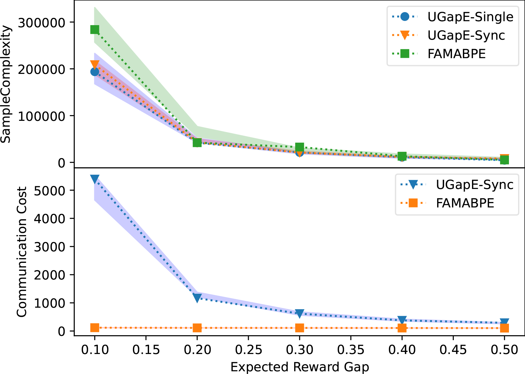
(a) MAB

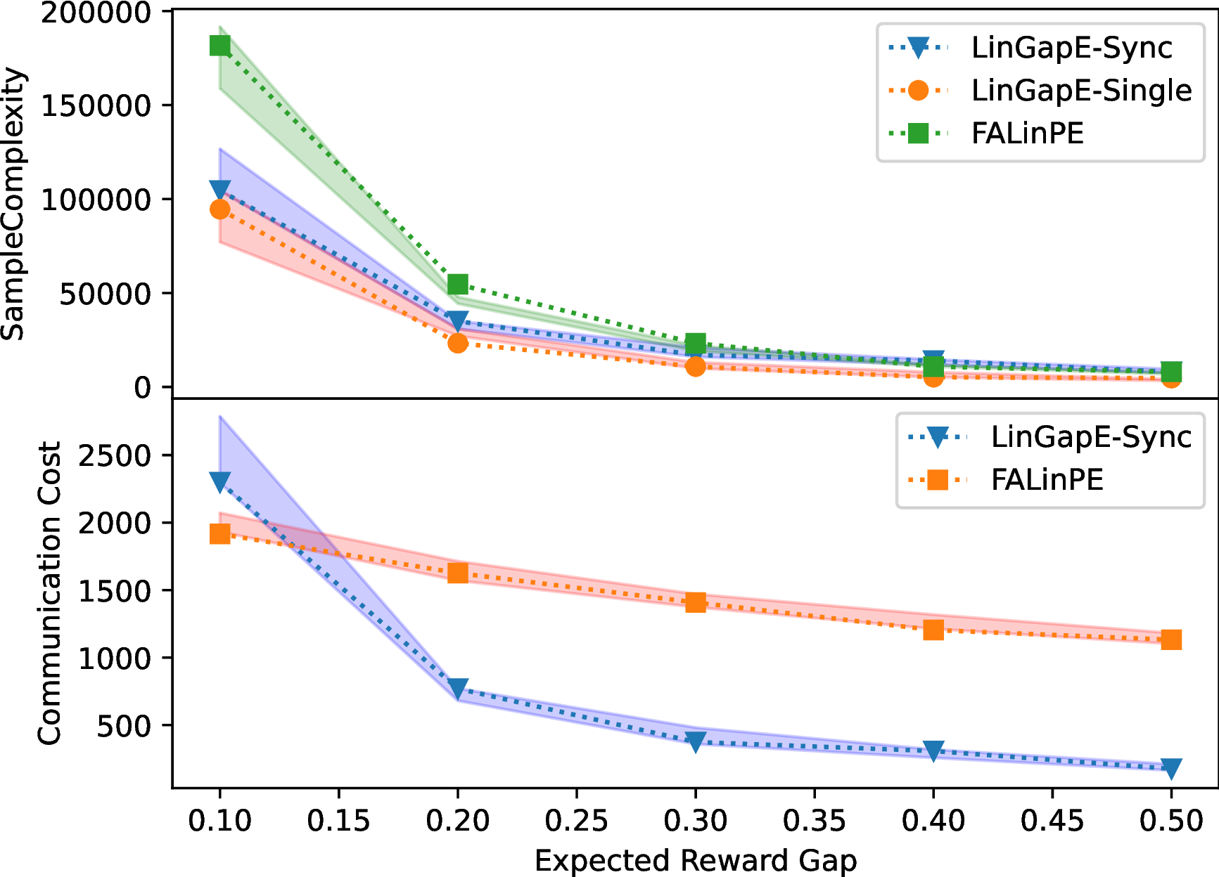
(b) Linear

Figure 1: Synthetic data: Experimental results for federated MAB and federated linear bandits.

We provide experiment results to empirically validate the communication and sample efficiency of FAMABPE and FALinPE. Our algorithms are compared with some baseline algorithms, in which the active agent would share its data with other agents via the server in every round. We would compare FAMABPE with single agent UGapEc and synchronous UGapEc [Gabillon et al., 2012] in the MAB setting. Besides, we would also compare FALinPE with single agent LinGapE and synchronous LinGapE [Xu et al., 2017]. We run the algorithms $10$ times and plot their average results.

6.1 Experiment Setup

MAB

We simulate the federated MAB in Section 3.1, with $\sigma=0.3$, $\delta=0.05$, $\epsilon=0$, $K=5$ and $M=10$. We sample the optimal arm from the uniform distribution and selectively sample the non-optimal arm to guarantee the reward gap. For synchronous UGapEc, we set the communication frequency as $100$ rounds. At the end of every $100$ rounds, the agents would upload their exploration results to the server and download other agents’ exploration results from the server. The communication cost of this naive synchronous algorithm is just $C(\tau)=\tau/50$, this is due to there are $\tau/(100M)$ communication episodes and in each episode agents would upload and download data for $2M$ times. The setup of FAMABPE follows Corollary 1 and in each round, the active agent $m_{t}$ is uniformly sampled from $\mathcal{M}$.

Linear bandits

Similar to the MAB case, we simulate the federated linear bandits with $d=5$ and other parameters are the same as the MAB setting. We first sample the model parameter $\boldsymbol{\theta}^{*}$ from a uniform distribution. Then, we sample the context of the optimal arm and selectively sample non-optimal arms to guarantee the reward gap. The synchronous LinGapE is similar to synchronous UGapEc. The setup of FALinPE follows Corollary 2 and the active agent in the linear case is also uniformly sampled from $\mathcal{M}$.

6.2 Experiment Results

MAB

The results of federated MAB are shown in Figure 1(a). All algorithms output their estimated best arms $\hat{k}^{*}=k^{*}$. We report the sample complexity and communication cost for the reward gap from $0.1$ to $0.5$. We can observe that the single agent which runs UGapEc achieved the smallest sample complexity. In comparison, the synchronous UGapEc would spend a slightly larger sample complexity when the gap equals $0.1$ and spend an almost identical cost when the gap equals $0.2$ to $0.5$. Compared with these baseline algorithms, our FAMABPE had a slightly larger sample complexity and can achieve the lowest communication cost. FAMABPE is the only algorithm that can achieve near-optimal sample complexity and efficient communication cost in a fully asynchronous environment.

Linear bandits

The results of federated linear bandits are provided in Figures 1(b). All algorithms output their estimated best arm $\hat{k}^{*}=k^{*}$. Similar to the MAB, we can observe that a single agent which runs LinGapE and synchronous LinGapE achieved the lowest sample complexity. In comparison, FALinPE required a relatively large sample complexity, especially when the gap equals $0.1$. Furthermore, the communication cost of synchronous LinGapE is larger than FALinPE when the gap equals $0.1$. Otherwise, smaller than FALinPE.

Experimental results on real-world data are provided in the appendix.

7 CONCLUSION

In this paper, we propose the first study on the pure exploration problem of both federated MAB and federated linear bandits in an asynchronous environment. First, we proposed an algorithm named FAMABPE, which can complete the $(\epsilon,\delta)$-pure exploration object of the federated MAB with $\tilde{O}(H^{M}_{\epsilon})$ sample complexity and $\tilde{O}(M^{3/2}K)$ communication cost using a novel event-triggered communication protocol. Then, we improved FAMABPE to FALinPE, which can finish the same object in the linear case with $\tilde{O}(H^{L}_{\epsilon}d)$ sample complexity and $\tilde{O}\big{(}\max(M^{2}d,M^{3/2}K)\big{)}$ communication cost. At the end of the paper, the effectiveness of the offered algorithms was further examined by the numerical simulation based on synthetic data and real-world data. In our future work, a potential direction is to investigate federated asynchronous pure exploration algorithms with a fixed budget.

Appendix A EXPERIMENTS ON REAL-WORLD DATA

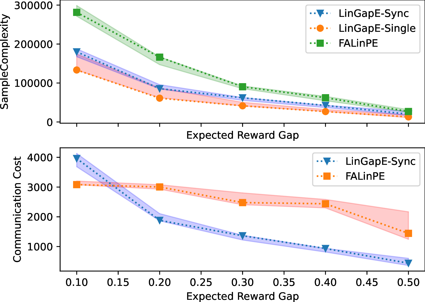
Figure 2: Experimental results on MovieLens for federated linear bandits.

In this section, we report an additional experiment on real-world dataset for federated linear bandits setting.

A.1 Experiment Setup

We use the MovieLens 20M dataset [Harper and Konstan, 2016] for the experiment. We follow [Li and Wang, 2022a] to preprocess the data and extract item features. Specifically, we keep users with over $3,000$ observations, which results in a dataset with $54$ users, $26567$ items (movies), and $214729$ interactions. For each item, we extract TF-IDF features from its associated tags and apply PCA to obtain item features with dimension $d=25$. We consider all items with non-zero ratings as positive feedback (reward $r=1$), and use ridge regression to learn $\boldsymbol{\theta}^{*}$ from extracted item features and their 0/1 rewards. To construct an arm set, we follow the same procedure as the simulation in Section 6 by first sampling an optimal arm and then selectively sampling non-optimal arms to guarantee the reward gap.

The baseline algorithms considered in this section are the same as those in the synthetic data case (Section 6). Besides, we set $d=25$, $K=10$, $\epsilon=0.05$, and other parameters of the federated linear bandits are also identical to Section 6. We report the average results of $10$ runs.

A.2 Experiment Results

The results of the federated linear bandits are shown in Figures 2. In each run, every algorithm could derive the best arm $k^{*}$. Similar to the results based on synthetic data, single agent LinGapE and synchronous LinGapE enjoyed the lowest sample complexity, and FALinPE spent a relatively large sample complexity. Besides, according to the tendency, FALinPE’s communication cost would be smaller than the synchronous LinGapE’s communication cost when the expected reward gap is smaller equals $0.15$. Note that synchronous LinGapE can only work in a synchronous environment, hence, FALinPE is the only known federated linear bandit algorithm that can simultaneously achieve near-optimal sample complexity and efficient communication cost in the fully asynchronous environment.

Appendix B NOTATIONS

$\mathcal{A}$	Arm set
$\mathcal{M}$	Agent set
$d$	Dimension of the model parameter and context
$\tau$	Sample complexity (stopping time)
$\mathcal{C}(\tau)$	Communication cost
$k^{*}$	Best arm
$\hat{k}^{*}$	Estimated best arm
$m_{t}$	Active agent in round $t$
$\eta_{m_{t},t}$	$\sigma$-sub-Gaussian noise
$r_{m_{t},t}$	Received reward of agent $m_{t}$ in round $t$
$k_{m_{t},t}$	Arm pulled by agent $m_{t}$ in round $t$
$\mu(k)$	Expected reward of arm $k$ in MAB
$\mathbb{x}_{k}$	Context of arm $k$
$\mathbb{y}(i,j)$	Context difference between $\mathbb{x}_{i}$ and $\mathbb{x}_{j}$
$\boldsymbol{\theta}^{*}$	Model parameter
$\delta$	Probability parameter of the fixed-confidence pure exploration problem
$\epsilon$	Reward gap parameter of the fixed-confidence pure exploration problem
$\gamma/\gamma_{1}/\gamma_{2}$	Triggered parameters
$\lambda$	Regularization parameter of the covariance matrix
$B(t)$	Breaking index
$\beta_{m_{t},t}(k)$	Exploration bonus of arm $k$ of the agent $m_{t}$ in FAMABPE
$\beta^{ser}_{t}(k)$	Exploration bonus of arm $k$ of the server in FAMABPE
$\alpha_{m_{t},t}(i,j)$	Exploration bonus of pair $(i,j)$ of the agent $m_{t}$ in FALinPE
$\alpha^{ser}_{t}(i,j)$	Exploration bonus of pair $(i,j)$ of the server in FALinPE
$\hat{\boldsymbol{\theta}}_{m_{t},t}$	Estimated model parameter of the agent $m_{t}$ in FALinPE
$\hat{\boldsymbol{\theta}}^{ser}_{t}$	Estimated model parameter of the server in FALinPE
$i_{m_{t},t}$	Empirical best arm of agent $m_{t}$ in round $t$
$j_{m_{t},t}$	Most ambiguous arm of agent $m_{t}$ in round $t$
$\Delta(i,j)$	Expected reward gap between arms $i$ and $j$
$\hat{\Delta}_{m_{t},t}(i,j)$	Estimated reward gap between arms $i$ and $j$ of the agent $m_{t}$
$\hat{\Delta}^{ser}_{t}(i,j)$	Estimated reward gap between arms $i$ and $j$ of the server
$\hat{\mu}_{m_{t},t}(k)$	Estimated reward of arm $k$ of the agent $m_{t}$ in FAMABPE
$\hat{\mu}^{ser}_{t}(k)$	Estimated reward of arm $k$ of the server in FAMABPE
$T_{m_{t},t}(k)$	Number of observations on arm $k$ that is available to the agent $m_{t}$ at $\tau$
$T^{ser}_{t}(k)$	Number of observations on arm $k$ that is available to the server at $\tau$
$T^{loc}_{m_{t},t}(k)$	Number of observations on arm $k$ has not been uploaded to the server by the agent $m_{t}$ at $t$
$T^{all}_{t}(k)$	Total number of observations on arm $k$
$\mathbb{V}_{m_{t},t}$	Covariance matrix of the agent $m_{t}$
$\mathbb{V}^{ser}_{t}$	Covariance matrix of the server
$\mathbb{V}^{loc}_{m_{t},t}$	Covariance matrix has not been uploaded to the server by the agent $m_{t}$
$\mathbb{V}^{all}_{t}$	Global covariance matrix
$H^{M}_{\epsilon}$	Problem complexity of the MAB
$H^{L}_{\epsilon}$	Problem complexity of the linear bandits

Appendix C PROOF OF THEOREM 1

For clarity, we here reintroduce the notations used in the proof. Recall that $T^{all}_{t}(k)$ denotes the total number of arm $k$ be pulled till round $t$, $T^{ser}_{t}(k)$ denotes the number of observations on arm $k$ that is available to the server at $t$, $T_{m,t}(k)$ denotes the the number of observations on arm $k$ that is available to the agent $m$ at $t$ and $T_{m,t}^{loc}(k)$ denotes the observations on arm $k$ of agent $m$ has not been uploaded to the server at $t$. Besides, $\hat{\Delta}_{t}^{ser}(i,j)$ and $\hat{\Delta}_{m,t}(i,j)$ denote the estimated reward gap between arm $i$ and $j$ of the agent $m$ and server in round $t$, respectively. Furthermore, we let $\beta_{m,t}(k)$ and $\beta^{ser}_{t}(k)$ denoting the exploration bonuses of the agent $m$ and server, respectively. Moreover, we define the reward estimator of arm $k$ of the agent $m$ and server as $\hat{\mu}_{m,t}(k)$ and $\hat{\mu}_{t}^{ser}(k)$, respectively.

Remark 6 (Global and local data in the federated MAB).

By the design of Algorithm 1, the total number of times arm $k$ has been pulled till round $t$ satisfies $T^{all}_{t}(k)=T^{ser}_{t}(k)+\sum_{m=1}^{M}T^{loc}_{m,t}(k)$, where $T^{ser}_{t}(k)$ denotes the number of observations on arm $k$ that has been uploaded to the server and $\sum_{m=1}^{M}T^{loc}_{m,t}(k)$ denotes the total number of observations on arm $k$ that agents $m=1,2,\dots,M$ have not uploaded to the server. Besides, as $T_{m,t}(k)$, $\forall m\in\mathcal{M},k\in\mathcal{A}$ is downloaded from the server in some round earlier than $t$, we have $T_{m,t}(k)\leq T^{ser}_{t}(k),\ \forall k\in\mathcal{A}$ and $\sum_{k=1}^{K}T_{m,t}(k)\leq\sum_{k=1}^{K}T^{ser}_{t}(k)$.

Proof sketch of Theorem 1

Proof of Theorem 1 consists of three main components: a) the communication cost $\mathcal{C}(\tau)$; b) the sample complexity $\tau$; c) the estimated best arm satisfies Eq (1). Specifically, to upper bound the total communications cost $\mathcal{C}(\tau)$, we utilize the property of the event-trigger (line 12 of Algorithm 1) that controls when the agents would communicate with the server (Lemma 1). To upper bound the sample complexity $\tau$, we first need to establish the relation between $\sum_{k=1}^{K}T^{ser}_{t}(k)$ and $\sum_{k=1}^{K}T^{loc}_{m,t}(k)$ based on the event triggered strategy (Lemma 4). Then, we establish exploration bonuses by $\sum_{k=1}^{K}T^{ser}_{t}(k)$ and $\sum_{k=1}^{K}T_{m,t}(k)$, $\forall k\in\mathcal{A},\ m\in\mathcal{M}$ and bound $T^{ser}_{\tau}(k)$, $\forall k\in\mathcal{A}$ accordingly (Lemma 2, 5 and 3). Finally, utilizing the relations given in Remark 6, we can bound $T^{all}_{\tau}(k)$, $\forall k\in\mathcal{A}$, and $\tau=\sum_{k=1}^{K}T^{all}_{\tau}(k)$. The guarantee of finding the best arm, i.e., Eq (1), directly follows the property of the breaking index, i.e., if $B(\tau)\leq\epsilon$, then $\Delta(k^{*},\hat{k}^{*})\leq\epsilon$ with probability at least $1-\delta$.

Detailed proof for the first two components are given in the following two subsections.

C.1 Upper Bound Communication Cost $\mathcal{C}(\tau)$

Lemma 1 (Communication cost).

Following the setting of Theorem 1, the total communication cost of FAMABPE can be bounded by

$$\mathcal{C}(\tau)\leq 2\Big{(}(M+1/\gamma)\log_{2}\tau\Big{)}.$$

Proof of Lemma 1.

The proof of this Lemma can be divided into two sections, in the first section, we would divide the sample complexity $\tau$ into $\log_{2}\tau$ episodes, then we would analyze the upper bound of the communication number of all agents in each episode. We define

$$\mathcal{T}_{i}=\min\Big{\{}t\in[K+1,\tau],\ \sum_{k=1}^{K}T^{ser}_{t}(k)\geq 2^{i}\Big{\}}$$

and the set of all rounds into episodes $i$ as $\{\mathcal{T}_{i},\mathcal{T}_{i}+1,...,\mathcal{T}_{i+1}-1\}$. According to the definition, we have $\sum_{k=1}^{K}T^{ser}_{\tau}(k)\leq\tau$, and thus

$$\max\{i\geq 0\}=\log_{2}\bigg{(}\sum_{k=1}^{K}T^{ser}_{\tau}(k)\bigg{)}\leq\log_{2}\tau.$$

We then prove $\forall i\geq 0$, from round $\mathcal{T}_{i}$ to $\mathcal{T}_{i+1}-1$, the communication number of all agents can be bounded by $M+1/\gamma$. We first define the communication number of agent $m$ from $\mathcal{T}_{i}$ to $\mathcal{T}_{i+1}-1$ as $\mathcal{N}_{m}$, the sequence of communication round of agent $m$ from round $\mathcal{T}_{i}$ to $\mathcal{T}_{i+1}-1$ as $t^{m}_{1},...,t^{m}_{\mathcal{N}_{m}}$, the communication number of all agents as $L$ and the sequence of all communication rounds from round $\mathcal{T}_{i}$ to $\mathcal{T}_{i+1}-1$ as $t_{i,1},...,t_{i,L}$. According to the communication condition (line 11 of Algorithm 1), we have $\forall m\in\mathcal{M},\ j\in|\mathcal{N}_{m}|$

$$\begin{split}\sum_{k=1}^{K}\Big{(}T_{m,t^{m}_{j}}(k)+T_{m,t^{m}_{j}}^{loc}(k)\Big{)}&>(1+\gamma)\sum_{k=1}^{K}T_{m,t^{m}_{j}}(k)\\ \sum_{k=1}^{K}T_{m,t^{m}_{j}}^{loc}(k)&>\gamma\sum_{k=1}^{K}T_{m,t^{m}_{j}}(k).\end{split}$$ (17)

Then, $\forall m\in\mathcal{M},\ j\in|\mathcal{N}_{m}|/\{1\}$, we have

$$\sum_{k=1}^{K}T_{m,t^{m}_{j}}^{loc}(k) >\gamma\sum_{k=1}^{K}T_{m,t^{m}_{j}}(k)\geq\gamma\sum_{k=1}^{K}T^{ser}_{\mathcal{T}_{i}}(k).$$ (18)

The inequality holds due to $T_{m,t^{m}_{j}}(k)=T^{ser}_{t^{m}_{j-1}}(k)$ and $t^{m}_{j-1}\geq\mathcal{T}_{i}$ when $j\in|\mathcal{N}_{m}|/\{1\}$. The above inequality implies $\forall t_{i,l}\geq t_{2}^{m_{t_{i,l}}}$

$$\begin{split}\sum_{k=1}^{K}\Big{(}T^{ser}_{t_{i,l}}(k)-T^{ser}_{t_{i,l-1}}(k)\Big{)}&\geq\sum_{k=1}^{K}\Big{(}T^{ser}_{t_{i,l-1}}(k)+T_{m_{t_{i,l}},t_{i,l}}^{loc}(k)\Big{)}-\sum_{k=1}^{K}T^{ser}_{t_{i,l-1}}(k)\\ &=\sum_{k=1}^{K}T_{m_{t_{i,l}},t_{i,l}}^{loc}(k)\\ &>\gamma\sum_{k=1}^{K}T_{m_{t_{i,l}},t_{i,l}}(k)\\ &\geq\gamma\sum_{k=1}^{K}T_{\mathcal{T}_{i}}^{ser}(k).\end{split}$$

Finally we can bound $L=\sum_{m=1}^{M}\mathcal{N}_{m}$

$$\begin{split}\sum_{k=1}^{K}\Big{(}T_{\mathcal{T}_{i+1}-1}^{ser}(k)-T_{\mathcal{T}_{i}}^{ser}(k)\Big{)}&=\sum_{l=1}^{L-1}\sum_{k=1}^{K}\Big{(}T^{ser}_{t_{i,l+1}}(k)-T^{ser}_{t_{i,l}}(k)\Big{)}\\ &\geq\gamma\sum_{m=1}^{M}(\mathcal{N}_{m}-1)\sum_{k=1}^{K}T_{\mathcal{T}_{i}}^{ser}(k).\end{split}$$ (19)

The last inequality holds owing to (17) and (18). With the definition of the episode, we have $\sum_{k=1}^{K}T_{\mathcal{T}_{i+1}-1}^{ser}(k)\leq 2\sum_{k=1}^{K}T_{\mathcal{T}_{i}}^{ser}(k)$. We can then rewrite equation (19) as

$$M+1/\gamma\geq\sum_{m=1}^{M}\mathcal{N}_{m}=L.$$

Due to one communication including one upload and one download, the communication cost in one episode is at most $2(M+1/\gamma)$ (following the definition of (2)). We can then bound the total communication cost

$$\mathcal{C}(\tau)\leq 2\Big{(}(M+1/\gamma)\log_{2}(\tau)\Big{)}.$$

∎

C.2 Upper Bound Sample Complexity $\tau$

Combining the breaking condition in Algorithm 1 (line 14$\sim$16), and the definition of $B(\tau)$, we have

$$\epsilon\geq B(\tau)=\hat{\Delta}^{ser}_{\tau}(j^{ser}_{\tau},i^{ser}_{\tau})+\beta^{ser}_{\tau}(i^{ser}_{\tau},j^{ser}_{\tau}).$$

Let’s first consider the case when the empirically best arm on the server side is not the optimal arm, i.e., $i^{ser}_{\tau}\not=k^{*}$. By the definition of $j^{ser}_{\tau}$, we have

$$\hat{\Delta}^{ser}_{\tau}(j^{ser}_{\tau},i^{ser}_{\tau})+\beta^{ser}_{\tau}(i^{ser}_{\tau},j^{ser}_{\tau})\geq\hat{\Delta}^{ser}_{\tau}(k^{*},i^{ser}_{\tau})+\beta^{ser}_{\tau}(i^{ser}_{\tau},k^{*}).$$

Recall that $\hat{k}^{*}=i^{ser}_{\tau}$ is the empirically best arm. Therefore, we have

$$\epsilon\geq\hat{\Delta}^{ser}_{\tau}(k^{*},\hat{k}^{*})+\beta^{ser}_{\tau}(\hat{k}^{*},k^{*})\geq\Delta(k^{*},\hat{k}^{*}),$$

where the second inequality is due to Lemma 2 below (proof of Lemma 2 is at the end of this section).

Lemma 2.

Following the setting of Theorem 1, we can establish the exploration bonuses

$$\begin{split}&\beta_{m_{t},t}(k)=\sigma\sqrt{\frac{2}{T_{m_{t},t}(k)}\log\bigg{(}\frac{4K}{\delta}\Big{(}(1+\gamma M)\sum_{k=1}^{K}T_{m_{t},t}(k)\Big{)}^{2}\bigg{)}}\\ &\beta^{ser}_{t}(k)=\sigma\sqrt{\frac{2}{T^{ser}_{t}(k)}\log\bigg{(}\frac{4K}{\delta}\Big{(}(1+\gamma M)\sum_{k=1}^{K}T^{ser}_{t}(k)\Big{)}^{2}\bigg{)}},\end{split}$$

for all $t\in[K+1,\tau]$, $k\in\mathcal{A}$, and the event

$$\mathcal{I}=\bigg{\{}\forall k\in\mathcal{A},\forall t\in[K+1,\tau],\ |\hat{\mu}_{m_{t},t}(k)-\mu(k)|\leq\beta_{m_{t},t}(k),\ |\hat{\mu}_{t}^{ser}(k)-\mu(k)|\leq\beta_{t}^{ser}(k)\bigg{\}}.$$

We have $\mathcal{P}(\mathcal{I})\geq 1-\delta$.

Furthermore, if $i^{ser}_{t}=k^{*}$, we have $\epsilon\geq\Delta(k^{*},\hat{k}^{*})=0$. The discussion above implies $\hat{k}^{*}$ output by FAMABPE satisfies the $(\epsilon,\delta)$-condition (1).

We now continue to bound the sample complexity $\tau$. First, we need to establish Lemma 3 below, which upper bounds $T_{\tau}^{ser}(k)$, the number of observations on arm $k$ that is available to the server at $\tau$.

Lemma 3.

Under the setting of Theorem 1, if event $\mathcal{I}$ happens, we can bound

$$T_{\tau}^{ser}(k)\leq\frac{2\sigma^{2}\log\Big{(}4K\Big{(}(1+M\gamma)\sum_{s=1}^{K}T^{ser}_{\tau}(s)\Big{)}^{2}/\delta\Big{)}}{\max\Big{(}\frac{\Delta(k^{*},k)+\epsilon}{3},\epsilon\Big{)}^{2}}+\gamma M\sum_{s=1}^{K}T^{ser}_{\tau}(s),\ \forall k\in\mathcal{A}.$$

With Lemma 3, we have

$$\begin{split}\sum_{k=1}^{K}T^{ser}_{\tau}(k)&\leq\sum_{k=1}^{K}\frac{2\sigma^{2}\log\Big{(}4K\Big{(}(1+\gamma M)\sum_{s=1}^{K}T^{ser}_{\tau}(s)\Big{)}^{2}/\delta\Big{)}}{\max\Big{(}\frac{\Delta(k^{*},k)+\epsilon}{3},\epsilon\Big{)}^{2}}+\gamma KM\sum_{s=1}^{K}T^{ser}_{\tau}(s)\\ &\leq\frac{1}{1-\gamma KM}\sum_{k=1}^{K}\frac{2\sigma^{2}\log\Big{(}4K\Big{(}(1+\gamma M)\sum_{s=1}^{K}T^{ser}_{\tau}(s)\Big{)}^{2}/\delta\Big{)}}{\max\Big{(}\frac{\Delta(k^{*},k)+\epsilon}{3},\epsilon\Big{)}^{2}}\\ &\leq\frac{1}{1-\gamma KM}\sum_{k=1}^{K}\frac{2\sigma^{2}\log\Big{(}4K\Big{(}(1+\gamma M)\tau\Big{)}^{2}/\delta\Big{)}}{\max\Big{(}\frac{\Delta(k^{*},k)+\epsilon}{3},\epsilon\Big{)}^{2}}.\end{split}$$

The last inequality is due to $\sum_{k=1}^{K}T^{ser}_{t}(k)\leq\tau$ (Remark 6). Based on the relation between $\tau$, $\sum_{m=1}^{M}\sum_{k=1}^{K}T^{loc}_{m,\tau}(k)$, and $\sum_{k=1}^{K}T^{ser}_{\tau}(k)$ (Remark 6), we have

$$\begin{split}\tau&=\sum_{k=1}^{K}T^{all}_{\tau}(k)=\sum_{k=1}^{K}T^{ser}_{\tau}(k)+\sum_{m=1}^{M}\sum_{k=1}^{K}T_{m,\tau}^{loc}(k)\\ &\leq\big{(}1+\gamma M\big{)}\sum_{k=1}^{K}T^{ser}_{\tau}(k)\\ &\leq\frac{1+\gamma M}{1-\gamma KM}\sum_{k=1}^{K}\frac{2\sigma^{2}\log\Big{(}4K\Big{(}(1+\gamma M)\tau\Big{)}^{2}/\delta\Big{)}}{\max\Big{(}\frac{\Delta(k^{*},k)+\epsilon}{3},\epsilon\Big{)}^{2}}\\ &=\frac{1+\gamma M}{1-\gamma KM}H^{M}_{\epsilon}2\log\Bigg{(}\frac{4K\Big{(}(1+\gamma M)\tau\Big{)}^{2}}{\delta}\Bigg{)},\end{split}$$ (20)

where the first inequality is due to Lemma 4, the second inequality is due to the inequality we established above, and the third is by definition of $H_{\epsilon}^{M}$.

Lemma 4.

Following the setting of Theorem 1, we have $\forall t\in[K+1,\tau]$

$$\sum_{k=1}^{K}T^{ser}_{t}(k)>1/\gamma\sum_{k=1}^{K}T^{loc}_{m_{t},t}(k).$$

Proof for Lemma 2, Lemma 3, and Lemma 4

In the following paragraphs, we provide the detailed proof for the lemmas used above.

Proof of Lemma 4.

For every round $t\in[K+1,\tau]$, if the agent $m_{t}$ communicates with the server at round $t$, we have

$$\sum_{k=1}^{K}T^{ser}_{t}(k)\geq 1/\gamma\sum_{k=1}^{K}T^{loc}_{m_{t},t}(k)=0.$$

The inequality holds by line 19 of Algorithm 1.

Else, according to the triggered condition of Algorithm 1, if agent $m_{t}$ does not communicate with the server in round $t$, we have

$$\begin{split}\sum_{k=1}^{K}(T_{m_{t},t}(k)+T_{m_{t},t}^{loc}(k))&\leq(1+\gamma)\sum_{k=1}^{K}T_{m_{t},t}(k)\\ \sum_{k=1}^{K}T_{m_{t},t}^{loc}(k)&\leq\gamma\sum_{k=1}^{K}T_{m_{t},t}(k).\end{split}$$

With the fact that $\sum_{k=1}^{K}T_{m_{t},t}(k)\leq\sum_{k=1}^{K}T^{ser}_{t}(k)$ (Remark 6), we can finally get

$$\sum_{k=1}^{K}T_{m_{t},t}^{loc}(k)\leq\gamma\sum_{k=1}^{K}T^{ser}_{t}(k).$$

Here we finish the proof of Lemma 4. ∎

Based on Lemma 4, we can prove Lemma 2 as shown below.

Proof of Lemma 2.

Due to $\hat{\mu}_{m_{t},t}(k)$ and $T_{m_{t},t}(k)$, $\forall k\in\mathcal{A},\ t\in[K+1,\tau]$ are all downloaded from the server and they would remain unchanged until the next round agent $m_{t}$ communicates with the server. This implies $\forall t_{1}\in[K+1,\tau]$, there exists a $t_{2}\in[K+1,\tau]$ which satisfies

$$\beta_{m_{t_{1}},t_{1}}(k)=\beta^{ser}_{t_{2}}(k)\ \text{and}\ \hat{\mu}_{m_{t_{1}},t_{1}}(k)=\hat{\mu}^{ser}_{t_{2}}(k),\ \forall k\in\mathcal{A}.$$

Hence, we can derive

$$\mathcal{P}(\mathcal{I})=\mathcal{P}\bigg{(}\forall k\in\mathcal{A},\forall t\in[K+1,\tau],\ |\hat{\mu}_{t}^{ser}(k)-\mu(k)|\leq\beta_{t}^{ser}(k)\bigg{)}.$$ (21)

We define $\mathcal{I}^{c}$ as the contradicted event of $\mathcal{I}$. Utilizing the union bound, it can be decomposed by

$$\mathcal{P}(\mathcal{I}^{c})\leq\sum_{k=1}^{K}\sum_{t=K+1}^{\tau}\mathcal{P}\bigg{(}|\hat{\mu}_{t}^{ser}(k)-\mu(k)|>\beta_{t}^{ser}(k)\bigg{)}.$$ (22)

With the help of the Hoeffeding inequality (Lemma 14), it has

$$\begin{split}\mathcal{P}\bigg{(}|\hat{\mu}_{t}^{ser}(k)-\mu(k)|>\beta_{t}^{ser}(k)\bigg{)}&\leq e^{-\beta_{t}^{ser}(k)^{2}T^{ser}_{t}(k)/2\sigma^{2}}\\ &=e^{-\log\big{(}\frac{4K}{\delta}\big{(}(1+\gamma M)\sum_{k=1}^{K}T^{ser}_{t}(k)\big{)}^{2}\big{)}}\\ &=\frac{\delta}{4K\big{(}(1+\gamma M)\sum_{k=1}^{K}T^{ser}_{t}(k)\big{)}^{2}}\\ &\leq\frac{\delta}{4Kt^{2}}.\end{split}$$ (23)

The first equality is owing to the definition of $\beta^{ser}_{t}(k)$ and the last inequality is owing to $t=\sum_{k=1}^{K}T^{ser}_{t}(k)+\sum_{m=1}^{M}\sum_{k=1}^{K}T^{loc}_{m,t}(k)\leq(1+\gamma M)\sum_{k=1}^{K}T^{ser}_{t}(k)$ (Lemma 4). Substituting the last term of (23) into (22), we can finally bound

$$\begin{split}\sum_{k=1}^{K}\sum_{t=K+1}^{\tau}\mathcal{P}\bigg{(}|\hat{\mu}_{t}^{ser}(k)-\mu(k)|>\beta_{t}^{ser}(k)\bigg{)}\leq\delta\end{split}$$

and $\mathcal{P}(\mathcal{I})=1-\mathcal{P}(\mathcal{I}^{c})\geq 1-\delta$. Here we finish the proof of Lemma 2. ∎

Before proving Lemma 3, we first need to establish Lemma 5 below.

Lemma 5.

We define $k^{ser}_{t}$ in round $t\in[K+1,\tau]$ as $k_{t}^{ser}=\arg\max_{k\in\{i_{t}^{ser},j_{t}^{ser}\}}\beta^{ser}_{t}(k)$. Following the setting of Theorem 1, if event $\mathcal{I}$ happens, we can bound the index $B(t)$ as

$$B(t)\leq\min\Big{(}0,-\Delta(k^{*},k_{t}^{ser})+4\beta_{t}^{ser}(k_{t}^{ser})\Big{)}+2\beta_{t}^{ser}(k_{t}^{ser}).$$ (24)

Proof of Lemma 5.

This proof follows the idea of Gabillon et al. [2012]. Consider the case when $i_{t}^{ser}=k^{*}$, we have

$$\begin{split}B(t)&=\hat{\Delta}^{ser}_{t}(j^{ser}_{t},i^{ser}_{t})+\beta^{ser}_{t}(i^{ser}_{t},j^{ser}_{t})\\ &\leq\hat{\Delta}^{ser}_{t}(j^{ser}_{t},i^{ser}_{t})+2\beta^{ser}_{t}(k^{ser}_{t})\\ &\leq\Delta(j^{ser}_{t},i^{ser}_{t})+4\beta^{ser}_{t}(k^{ser}_{t})\\ &=-\Delta(k^{*},j^{ser}_{t})+4\beta^{ser}_{t}(k^{ser}_{t})\\ &\leq-\Delta(k^{*},k^{ser}_{t})+4\beta^{ser}_{t}(k^{ser}_{t}),\end{split}$$ (25)

where the first inequality is owing to the definition of $k^{ser}_{t}$ and the second inequality is owing to the definition of the event $\mathcal{I}$. Then, consider the case when $j^{ser}_{t}=k^{*}$, we have

$$\begin{split}B(t)&=\hat{\Delta}^{ser}_{t}(j^{ser}_{t},i^{ser}_{t})+\beta^{ser}_{t}(i^{ser}_{t},j^{ser}_{t})\\ &\leq\hat{\Delta}^{ser}_{t}(j^{ser}_{t},i^{ser}_{t})+2\beta^{ser}_{t}(k^{ser}_{t})\\ &\leq-\hat{\Delta}^{ser}_{t}(j^{ser}_{t},i^{ser}_{t})+2\beta^{ser}_{t}(k^{ser}_{t})\\ &\leq-\Delta(j^{ser}_{t},i^{ser}_{t})+4\beta^{ser}_{t}(k^{ser}_{t})\\ &=-\Delta(k^{*},i^{ser}_{t})+4\beta^{ser}_{t}(k^{ser}_{t})\\ &\leq-\Delta(k^{*},k^{ser}_{t})+4\beta^{ser}_{t}(k^{ser}_{t}),\end{split}$$ (26)

where the second inequality is owing to the definition of the $i_{t}^{ser}$ (line 13 of Algorithm 1).

Combine (25) and (26), it yields

$$B(t)\leq-\Delta(k^{*},k^{ser}_{t})+4\beta_{t}^{ser}(k_{t}^{ser}),$$ (27)

when $i^{ser}_{t}=k^{*}$ or $j^{ser}_{t}=k^{*}$. Furthermore, due to $B(t)=\hat{\Delta}^{ser}_{t}(j^{ser}_{t},i^{ser}_{t})+\beta^{ser}_{t}(j^{ser}_{t},i^{ser}_{t})$ and $\hat{\Delta}^{ser}_{t}(j^{ser}_{t},i^{ser}_{t})\leq 0$, we can derive $B(t)\leq\beta^{ser}_{t}(j^{ser}_{t},i^{ser}_{t})\leq 2\beta^{ser}_{t}(k^{ser}_{t})$. In the light of (27), we can finally get

$$B(t)\leq\min\Big{(}0,\Delta(k^{*},k^{ser}_{t})+2\beta_{t}^{ser}(k_{t}^{ser})\Big{)}+2\beta_{t}^{ser}(k_{t}^{ser}).$$ (28)

We further consider the case when $i_{t}^{ser}\not=k^{*}$ and $j_{t}^{ser}\not=k^{*}$, then we can derive

$$\begin{split}B(t)&=\hat{\Delta}^{ser}_{t}(j^{ser}_{t},i^{ser}_{t})+\beta^{ser}_{t}(i^{ser}_{t},j^{ser}_{t})\\ &\leq\Delta(j^{ser}_{t},i^{ser}_{t})+2\beta^{ser}_{t}(i^{ser}_{t},j^{ser}_{t})\\ &=\Delta(j^{ser}_{t},k^{*})+\Delta(k^{*},i^{ser}_{t})+2\beta^{ser}_{t}(i^{ser}_{t},j^{ser}_{t})\\ &\leq\Delta(j^{ser}_{t},k^{*})+3\beta^{ser}_{t}(i^{ser}_{t},j^{ser}_{t})\\ &\leq\Delta(j^{ser}_{t},k^{*})+6\beta^{ser}_{t}(k^{ser}_{t})\\ &=-\Delta(k^{*},j^{ser}_{t})+6\beta^{ser}_{t}(k^{ser}_{t}),\end{split}$$ (29)

where the second equality is owing to $\Delta(i^{ser}_{t},j^{ser}_{t})=\Delta(i^{ser}_{t},k^{*})+\Delta(k^{*},j^{ser}_{t})$ and second inequality is owing to

$$\begin{split}\beta_{t}^{ser}(i_{t}^{ser},j^{ser}_{t})&\geq\hat{\Delta}^{ser}_{t}(j^{ser}_{t},i^{ser}_{t})+\beta^{ser}_{t}(i^{ser}_{t},j^{ser}_{t})\\ &\geq\hat{\Delta}^{ser}_{t}(k^{*},i^{ser}_{t})+\beta^{ser}_{t}(i^{ser}_{t},k^{*})\\ &\geq\Delta(k^{*},i^{ser}_{t}).\end{split}$$

Similar to (29), we also can show

$$\begin{split}B(t)&=\hat{\Delta}^{ser}_{t}(j^{ser}_{t},i^{ser}_{t})+\beta^{ser}_{t}(i^{ser}_{t},j^{ser}_{t})\\ &\leq\beta^{ser}_{t}(i^{ser}_{t},j^{ser}_{t})\\ &\leq-\Delta(k^{*},i^{ser}_{t})+\hat{\Delta}^{ser}_{t}(k^{*},i^{ser}_{t})+\beta^{ser}_{t}(k^{*},i^{ser}_{t})+\beta^{ser}_{t}(i^{ser}_{t},j^{ser}_{t})\\ &\leq-\Delta(k^{*},i^{ser}_{t})+\hat{\Delta}^{ser}_{t}(j^{ser}_{t},i^{ser}_{t})+\beta^{ser}_{t}(j^{ser}_{t},i^{ser}_{t})+\beta^{ser}_{t}(i^{ser}_{t},j^{ser}_{t})\\ &\leq-\Delta(k^{*},i^{ser}_{t})+4\beta^{ser}_{t}(k^{ser}_{t}).\end{split}$$ (30)

The second inequality is due to the definition of the even $\mathcal{I}$ and the third inequality is due to the definition of the $j_{t}^{ser}$.

Combine (29) and (30), it yields

$$B(t)\leq-\Delta(k^{*},k_{t}^{ser})+6\beta_{t}^{ser}(k_{t}^{ser})$$ (31)

when $i^{ser}_{t}\not=k^{*}$ and $j^{ser}_{t}\not=k^{*}$. In the light of (31), we can finally get

$$B(t)\leq\min\Big{(}0,-\Delta(k^{*},k^{ser}_{t})+4\beta_{t}^{ser}(k_{t}^{ser})\Big{)}+2\beta_{t}^{ser}(k_{t}^{ser}).$$ (32)

Combine (28) and (32), then we can finish the proof of Lemma 2. ∎

Proof of Lemma 3.

Suppose agent $m$ communicates in round $t_{1}$ and $t_{2}$, then from round $t\in[t_{1}+1,t_{2}]$, owing to $\hat{\mu}_{m,t}(k)$ and $T_{m,t}(k)$ remain unchanged, $k_{m,t}$ would not change either (we highlight this knowledge in Remark 1). We define at round $t_{k}\not=\tau$, an agent $m$ communicates with the server and $k^{ser}_{t_{k}}=k$, $\forall k\in\mathcal{A}$ (the definition of the $k^{ser}_{t}$ is provided in Lemma 5). And after round $t_{k}$, when any agent communicating with the server, $k^{ser}_{t}\not=k$. This implies

$$\begin{split}T_{\tau}^{ser}(k)\leq&T_{m,t_{k}+1}(k)+(\gamma M)\sum_{s=1}^{K}T_{\tau}^{ser}(s)\\ =&T^{ser}_{t_{k}}(k)+(\gamma M)\sum_{s=1}^{K}T_{\tau}^{ser}(s).\end{split}$$ (33)

The inequality holds due to for $t\in[t_{k}+1,\tau]$, $\forall m\in\mathcal{M}$ would upload $T_{m,t}^{loc}(k)>0$ to the server at most one time (according to the definition of $t_{k}$) and $T_{m,t}^{loc}(k)\leq\sum_{s=1}^{K}T_{m,t}^{loc}(s)\leq\gamma\sum_{s=1}^{K}T^{ser}_{\tau}(s)$ according to $t\leq\tau$ and the Lemma 4.

We would further bound $T^{ser}_{t_{k}}(k)=T_{m,t_{k}+1}(k)$. According to agent $m$ sets $k^{ser}_{t_{k}}=k$ and the definition of the breaking condition (line 14$\sim$16 in Algorithm 1), with Lemma 5, we can derive

$$\begin{split}\epsilon&\leq B(t_{k})\\ &\leq\min\Big{(}0,-\Delta(k^{*},k)+4\beta_{t_{k}}^{ser}(k)\Big{)}+2\beta_{t_{k}}^{ser}(k).\end{split}$$ (34)

Substituting (6) into (34), we have

$$T^{ser}_{t_{k}}(k)\leq\frac{2\sigma^{2}\log\Big{(}4K\Big{(}(1+\gamma M)\sum_{s=1}^{K}T^{ser}_{t_{k}}(s)\Big{)}^{2}/\delta\Big{)}}{\max\Big{(}\frac{\Delta(k^{*},k)+\epsilon}{3},\epsilon\Big{)}^{2}}.$$

With (33) and $t_{k}<\tau$, we can finally bound $T^{ser}_{\tau}(k)$, i.e.

$$\begin{split}T^{ser}_{\tau}(k)&\leq\frac{2\sigma^{2}\log\Big{(}4K\Big{(}(1+\gamma M)\sum_{s=1}^{K}T^{ser}_{\tau}(s)\Big{)}^{2}/\delta\Big{)}}{\max\Big{(}\frac{\Delta(k^{*},k)+\epsilon}{3},\epsilon\Big{)}^{2}}+\gamma M\sum_{s=1}^{K}T^{ser}_{\tau}(s).\end{split}$$

Here we finish the proof of Lemma 3. ∎

Appendix D PROOF OF COROLLARY 1

Proof of Corollary 1.

Let $\tau^{\prime}$ be a parameter that satisfies

$$\tau^{\prime}\leq\tau=\frac{M+\sqrt{M}/K}{M-\sqrt{M}}H^{M}_{\epsilon}2\log\Bigg{(}\frac{4K\Big{(}(1+1/(M^{1/2}K))\tau^{\prime}\Big{)}^{2}}{\delta}\Bigg{)}.$$

Due to the fact that $\sqrt{x}\geq\log(x)$ holds when $x>0$, we have

$$\begin{split}\tau^{\prime}&\leq\frac{M+\sqrt{M}/K}{M-\sqrt{M}}H^{M}_{\epsilon}2\log\bigg{(}\Big{(}\frac{4K(1+1/(M^{1/2}K))\tau^{\prime}}{\delta^{1/2}}\Big{)}^{2}\bigg{)}\\ &\leq\frac{M+\sqrt{M}/K}{M-\sqrt{M}}H^{M}_{\epsilon}4\sqrt{\frac{4K(1+1/(M^{1/2}K))\tau^{\prime}}{\delta^{1/2}}}\\ &\leq\bigg{(}\frac{M+\sqrt{M}/K}{M-\sqrt{M}}H^{M}_{\epsilon}4\bigg{)}^{2}\frac{4K(1+1/(M^{1/2}K))}{\delta^{1/2}}.\\ \end{split}$$ (35)

We define the last term of (35) as $\Lambda$. Then based on (20) and (35), we can finally get

$$\begin{split}\tau\leq&\frac{M+\sqrt{M}/K}{M-\sqrt{M}}H^{M}_{\epsilon}2\log\Bigg{(}\frac{4K\Big{(}(1+1/(M^{1/2}K))\Lambda\Big{)}^{2}}{\delta}\Bigg{)},\end{split}$$ (36)

where

$$\Lambda=\bigg{(}\frac{M+\sqrt{M}/K}{M-\sqrt{M}}H^{M}_{\epsilon}4\bigg{)}^{2}\frac{4K(1+1/(M^{1/2}K))}{\delta^{1/2}}.$$

In the light of Lemma 1, setting of the Theorem 1 and (36), we can bound the communication cost

$$\mathcal{C}(\tau)=O\Big{(}KM^{3/2}\log_{2}(H^{M}_{\epsilon})\Big{)}.$$ (37)

Here we finish the proof of Corollary 1. ∎

Appendix E PROOF OF THEOREM 2

Lemma 6.

Given $\delta\in(0,1)$ and any pure algorithm $\mathbb{Alg}$. For a hard-to-learn MAB instance $\boldsymbol{\pi}$ and some $c>0$, the expected sample complexity can be lower bounded by $\mathds{E}^{\mathbb{Alg}}_{\boldsymbol{\pi}}[\tau]\geq\sum_{k=1}^{K}c\log(1/\delta)/(\Delta(k^{*},k)+\epsilon)^{2}$. $\mathds{E}^{\textbf{Alg}}_{\boldsymbol{\pi}}[.]$ denotes the expectation under the algorithm Alg and the problem instance $\boldsymbol{\pi}$.

Proof of Lemma 6.

This proof can directly derive from Lemma 1 of Kaufmann et al. [2014]. Using the fact that the KL divergence between two unit-variance Gaussian distributions with means $\mu^{\prime}$ and $\mu$ satisfy $KL(\mu,\mu^{\prime})=(\mu-\mu^{\prime})^{2}/2$, we can derive

$$\sum_{k=1}^{K}\mathds{E}_{\boldsymbol{\pi}}^{\mathbb{Alg}}[T^{all}_{\tau}(k)](\mu^{\prime}(k)-\mu(k))^{2}\geq 2\ln\Big{(}\frac{1}{2.4\delta}\Big{)}$$ (38)

for all $\boldsymbol{\pi}^{\prime}=[\mu^{\prime}(k):k\in[K]]\in\mathbb{Alt}$, where $\mathbb{Alt}=\{\boldsymbol{\pi}^{\prime}\in\mathcal{R}^{K}:\boldsymbol{\pi}\not=\boldsymbol{\pi}^{\prime}\}$.

Let’s fix an arbitrary $\epsilon\geq 0$ and $k\in[K]$. Consider a instance $\boldsymbol{\pi}^{\prime}=[\mu^{\prime}(k):k\in[K]]$ with $\mu^{\prime}(k^{\prime})=\mu(k^{\prime})$, $\forall k^{\prime}\in[K]/k$ and $\mu^{\prime}(k)=\mu(k^{*})+\epsilon$. Substituting $\boldsymbol{\pi}^{\prime}$ into (38), we have

$$\mathds{E}_{\boldsymbol{\pi}}^{\mathbb{Alg}}[T^{all}_{\tau}(k)](\mu(k^{*})+\epsilon-\mu(k))^{2}\geq 2\ln\Big{(}\frac{1}{2.4\delta}\Big{)}$$

and

$$\mathds{E}_{\boldsymbol{\pi}}^{\mathbb{Alg}}[T^{all}_{\tau}(k)]\geq\frac{2}{(\Delta(k^{*},k)+\epsilon)^{2}}\ln\Big{(}\frac{1}{2.4\delta}\Big{)}.$$

Due to $\tau=\sum_{k=1}^{K}T^{all}_{\tau}(k)$, the expected sample complexity can be finally lower bounded by

$$\mathds{E}_{\boldsymbol{\pi}}^{\mathbb{Alg}}[\tau]\geq\sum_{k=1}^{K}\frac{2}{(\Delta(k^{*},k)+\epsilon)^{2}}\ln\Big{(}\frac{1}{2.4\delta}\Big{)}.$$ (39)

Here we finish the proof of Lemma 6. ∎

Proof of Theorem 2.

For any algorithm $\mathbb{FedAlg}$ for federated asynchronous pure exploration on MAB, we design the auxiliary algorithm $\mathbb{Aux}$ following Wang et al. [2019], He et al. [2022]: For each agent $m\in\mathcal{M}$, it would execute algorithm $\mathbb{FedAlg}$ until there is a communication between $m$ and the server. After the communication, $m$ would forget all information and execute a single agent algorithm $\mathbb{SinAlg}$. Algorithm $\mathbb{SinAlg}$ satisfies for any MAB instance $\boldsymbol{\pi}=[\mu(k):k\in[K]]$, $\mathbb{SinAlg}$ can output an estimated best arm that satisfies (1) and its expected sample complexity can be upper bounded by $\mathds{E}^{\mathbb{SinAlg}}_{\boldsymbol{\pi}}[\tau]\leq\sum_{k=1}^{K}\mathcal{C}\log(1/\delta))/(\Delta(k^{*},k)+\epsilon)^{2}$, where $\mathcal{C}>0$ is a constant. In this case, for each agent $m\in\mathcal{M}$, $\mathbb{Aux}$ would not derive any information from other agents and it will reduce to a single agent algorithm.

We suppose agents would be active in a round-robin manner, i.e., agent would be active from the agent $1$ to agent $K$, and so on. According to the previous discussion and Lemma 6, the $\mathbb{Aux}$ algorithm is reduced to a single agent algorithm, and the expected sample complexity of agent $m$ with $\mathbb{Aux}$ can be lower bounded by

$$\mathds{E}^{\mathbb{Aux},m}[\tau]\geq\sum_{k=1}^{K}\frac{c\log(1/\delta)}{(\Delta(k^{*},k)+\epsilon)^{2}},\ \forall m\in\mathcal{M}.$$ (40)

Based on (40), it is easy to lower bound the total expected sample complexity of $\mathbb{Aux}$

$$\mathds{E}^{\mathbb{Aux}}[\tau]=\sum_{m=1}^{M}\mathds{E}^{\mathbb{Aux},m}[\tau]\geq M\sum_{k=1}^{K}\frac{c\log(1/\delta)}{(\Delta(k^{*},k)+\epsilon)^{2}}.$$ (41)

For each agent $m\in\mathcal{M}$, let $p_{m}$ denote the probability that agent $m$ will communicate with the server. Notice that before the communication, $\mathbb{Aux}$ has the same performance as $\mathbb{FedAlg}$, while after the communication, $\mathbb{Aux}$ performs the $\mathbb{SinAlg}$ algorithm. Based on the definition of $\mathbb{SinAlg}$ and (40), the expected sample complexity for agent $m$ with $\mathbb{Aux}$ can be upper bounded by

$$\mathds{E}^{\mathbb{Aux},m}[\tau]\leq\mathds{E}^{\mathbb{FedAlg},m}[\tau]+p_{m}\sum_{k=1}^{K}\frac{\mathcal{C}\log(1/\delta)}{(\Delta(k^{*},k)+\epsilon)^{2}}.$$ (42)

Based on (42), we can finally upper bound the sample complexity of $\mathbb{Aux}$ as

$$\begin{split}\mathds{E}^{\mathbb{Aux}}[\tau]&=\sum_{m=1}^{M}\mathds{E}^{\mathbb{Aux},m}[\tau]\\ &\leq\sum_{m=1}^{M}\mathds{E}^{\mathbb{FedAlg},m}[\tau]+\Big{(}\sum_{p=1}^{M}p_{m}\Big{)}\sum_{k=1}^{K}\frac{\mathcal{C}\log(1/\delta)}{(\Delta(k^{*},k)+\epsilon)^{2}}\\ &\leq\mathds{E}^{\mathbb{FedAlg}}[\tau]+\Big{(}\sum_{p=1}^{M}p_{m}\Big{)}\sum_{k=1}^{K}\frac{\mathcal{C}\log(1/\delta)}{(\Delta(k^{*},k)+\epsilon)^{2}}.\end{split}$$ (43)

Substituting (41) into (43), for any asynchronous federated pure exploration algorithm with expected communication cost $\sum_{p=1}^{M}p_{m}\leq(c/2\mathcal{C})M=O(M)$, we have

$$\begin{split}\mathds{E}^{\mathbb{FedAlg}}[\tau]&\geq M\sum_{k=1}^{K}\frac{c\log(1/\delta)}{(\Delta(k^{*},k)+\epsilon)^{2}}-\Big{(}\sum_{p=1}^{M}p_{m}\Big{)}\sum_{k=1}^{K}\frac{\mathcal{C}\log(1/\delta)}{(\Delta(k^{*},k)+\epsilon)^{2}}\\ &\geq\frac{M}{2}\sum_{k=1}^{K}\frac{c\log(1/\delta)}{(\Delta(k^{*},k)+\epsilon)^{2}}.\end{split}$$ (44)

Here we finish the proof of Theorem 2. ∎

Appendix F PROOF OF THEOREM 3

Recall that the upper confidence bounds of the agent $m$ and server are defined as $\alpha_{m,t}(i,j)=\|\mathbb{y}(i,j)\|_{\mathbb{V}_{m_{t},t}^{-1}}C_{m,t}$ and $\alpha_{t}^{ser}(i,j)=\|\mathbb{y}(i,j)\|_{\mathbb{V}_{t}^{ser^{-1}}}C_{t}^{ser}$, respectively. The estimated model parameters of the agent $m$ and server are denoted as $\hat{\boldsymbol{\theta}}_{m,t}$ and $\hat{\boldsymbol{\theta}}^{ser}_{t}$, respectively. Besides, we also provide the Remark 7 to specifically illustrate the relationship between some most important data used in the proof of Theorem 3.

Remark 7 (Global and local data of the linear case).

Due to the transmitted data in the linear case being more complicated than the data in MAB. We here provide new notations to clarify the relations between global data and local data. The following matrix and vector denote the global data

$$\begin{split}&\mathbb{V}_{t}^{all}=\lambda\mathbb{I}+\sum_{s=1}^{t}\mathbb{x}_{m_{s},s}\mathbb{x}_{m_{s},s}^{\top}=\mathbb{V}^{ser}_{t}+\sum_{m=1}^{M}\mathbb{V}^{loc}_{m,t},\\ &\mathbb{b}_{t}^{all}=\sum_{s=1}^{t}\mathbb{x}_{m_{s},s}r_{m_{s},s}=\mathbb{b}^{ser}_{t}+\sum_{m=1}^{M}\mathbb{b}^{loc}_{m,t},\\ &T^{all}_{t}(k)=\sum_{s=1}^{t}\mathds{1}\{k=k_{m_{s},s}\}=T^{ser}_{t}(k)+\sum_{m=1}^{M}T^{loc}_{m,t}(k),\ \forall k\in\mathcal{A}.\end{split}$$

We define $N_{m,t}$ as the final round when agent $m$ communicates with the server at the end of round $t$. The collected data of agent $m$ that has not been uploaded to the server is provided as follows

$$\begin{split}&\mathbb{V}_{m,t}^{loc}=\sum_{s=N_{m,t}+1}^{t}\mathds{1}\{m_{s}=m\}\mathbb{x}_{m_{s},s}\mathbb{x}_{m_{s},s}^{\top},\\ &\mathbb{b}_{m,t}^{loc}=\sum_{s=N_{m,t}+1}^{t}\mathds{1}\{m_{s}=m\}\mathbb{x}_{m_{s},s}r_{m_{s},s}\\ &T^{loc}_{m,t}(k)=\sum_{s=N_{m,t}+1}^{t}\mathds{1}\{m_{s}=m,k=k_{m_{s},s}\},\ \forall k\in\mathcal{A}.\end{split}$$

Similarly, the data that has been uploaded to the server yields

$$\begin{split}&\mathbb{V}_{t}^{ser}=\lambda\mathbb{I}+\sum_{m=1}^{M}\sum_{s=1}^{N_{m,t}}\mathds{1}\{m_{s}=m\}\mathbb{x}_{m_{s},s}\mathbb{x}_{m_{s},s}^{\top},\\ &\mathbb{b}_{t}^{ser}=\sum_{m=1}^{M}\sum_{s=1}^{N_{m,t}}\mathds{1}\{m_{s}=m\}\mathbb{x}_{m_{s},s}r_{m_{s},s}\\ &T^{ser}_{t}(k)=\sum_{m=1}^{M}\sum_{s=1}^{N_{m,t}}\mathds{1}\{m_{s}=m,k=k_{m_{s},s}\},\ \forall k\in\mathcal{A}.\end{split}$$

According to the communication protocol, the local data of every agent $m\in\mathcal{M}$ can be represented by

$$\begin{split}\mathbb{V}_{m,t}=\mathbb{V}^{ser}_{N_{m,t}},\ \mathbb{b}_{m,t}=\mathbb{b}^{ser}_{N_{m,t}},\ T_{m,t}(k)=T^{ser}_{N_{m,t}}(k),\ \forall k\in\mathcal{A}.\end{split}$$

Accordingly, we have $V_{m,t}\preceq V^{ser}_{t}$ and $\sum_{k=1}^{K}T_{m,t}(k)\leq\sum_{k=1}^{K}T^{ser}_{t}(k)$, $\forall t\in[K+1,\tau]$.

Proof sketch of Theorem 3

The proof of Theorem 3 also consists of three main components, i.e., a) the sample complexity $\tau$; b) the communication cost $\mathcal{C}(\tau)$; c) the estimated best arm satisfies Eq (1). Specifically, to upper bound the total communication cost $C(\tau)$, we utilize the property that the agents communicating with the server when at least one of the two events (line 11 of Algorithm 2) is triggered (Lemma 7). To upper bound the sample complexity $\tau$, we first establish the relationship between $\sum_{k=1}^{K}T^{ser}_{t}(k)$ and $\sum_{k=1}^{K}T^{loc}_{m,t}(k)$ and the relationship between $\mathbb{V}^{ser}_{t}$ and $\mathbb{V}^{loc}_{m,t}$ based on the hybrid event triggered strategy (Lemma 10). Then, we design the exploration bonuses by $\sum_{k=1}^{K}T_{m_{t},t}(k)$, $\mathbb{V}_{m_{t},t}$, $\sum_{k=1}^{K}T^{ser}_{t}(k)$ and $\mathbb{V}^{ser}_{t}$ (Lemma 8). Furthermore, we bound the matrix norms $\|\mathbb{y}(i,j)\|_{\mathbb{V}^{-1}_{m_{t},t}}$ and $\|\mathbb{y}(i,j)\|_{\mathbb{V}^{ser^{-1}}_{t}}$, $\forall i,j\in\mathcal{A}$ based on the arm selection strategy (Lemma 11). Combine these knowledge, we can bound $T^{ser}_{\tau}(k)$, $\forall k\in\mathcal{A}$ (Lemma 12 and 9). Finally, utilizing the knowledge of Remark 7, we can bound $T^{all}_{\tau}(k)$, $\forall k\in\mathcal{A}$, and $\tau=\sum_{k=1}^{K}T^{all}_{\tau}(k)$. Similar to the MAB setting, the guarantee on finding the best arm directly follows the property of the breaking index, i.e., if $B(\tau)\leq\epsilon$, then $\Delta(k^{*},\hat{k}^{*})\leq\epsilon$ with probability at least $1-\delta$.

F.1 Upper Bound Communication Cost $\mathcal{C}(\tau)$

Lemma 7 (Communication cost of the hybrid event-triggered strategy in Algorithm 2).

Under the setting of Theorem 3, the total triggered number of the first event (line 11 of Algorithm 2) can be bounded by

$$(M+1/\gamma_{1})d\log_{2}\Big{(}1+\frac{\tau}{\lambda d}\Big{)}$$ (45)

and the total triggered number of the second event can be bounded by

$$(M+1/\gamma_{2})\log_{2}(\tau).$$

The total communication cost can be bounded by

$$\mathcal{C}(\tau)\leq 2\Bigg{(}(M+1/\gamma_{1})d\log_{2}\bigg{(}1+\frac{\tau}{\lambda d}\bigg{)}+(M+1/\gamma_{2})\log_{2}(\tau)\Bigg{)}.$$

Proof of Lemma 7.

The triggered number of the second event can be bounded by Lemma 1. Besides, we can bound the triggered number of the first event similar to He et al. [2022]. The proof of (45) also can be divided into two sections, in the first section, we would divide the sample complexity $\tau$ into $\log_{2}(1+\tau/\lambda d)$ episodes, then we would analysis the upper bound of the triggered number of the first event in each episode. We define

$$\mathcal{T}_{i}=\min\Big{\{}t\in|\tau|,\ \text{det}(\mathbb{V}^{ser}_{t})\geq 2^{i}\lambda^{d}\Big{\}}$$

and the set of all rounds into episodes $\{\mathcal{T}_{i},\mathcal{T}_{i}+1,...,\mathcal{T}_{i+1}-1\}$, $\forall i\geq 0$. By the Lemma 15, we can bound

$$\text{det}(V^{ser}_{\tau})\leq\lambda^{d}\Big{(}1+\frac{\tau}{\lambda d}\Big{)}^{d}.$$

Accordingly, the number of the episode can be bounded by

$$\max\{i\geq 0\}=\log_{2}\bigg{(}\frac{\text{det}(\mathbb{V}^{ser}_{\tau})}{\lambda^{d}}\bigg{)}\leq d\log_{2}\Big{(}1+\frac{\tau}{\lambda d}\Big{)}.$$

We then prove $\forall i\geq 0$, from round $\mathcal{T}_{i}$ to $\mathcal{T}_{i+1}-1$, the triggered number of the first event can be bounded by $M+1/\gamma_{1}$. We first define the number of agents $m$ triggers the first event in $\mathcal{T}_{i}$ to $\mathcal{T}_{i+1}-1$ as $\mathcal{N}_{m}$, the sequence of agent $m$ triggers the first event in round $\mathcal{T}_{i}$ to $\mathcal{T}_{i+1}-1$ as $t^{m}_{1},...,t^{m}_{\mathcal{N}_{m}}$, the number of every agent triggers the first event in $\mathcal{T}_{i}$ to $\mathcal{T}_{i+1}-1$ as $L$ and the sequence of the first event be triggered in $\mathcal{T}_{i}$ to $\mathcal{T}_{i+1}-1$ as $t_{i,1},...,t_{i,L}$. According to the definition of the first event, we have

$$\text{det}(\mathbb{V}_{m_{t},t}+\mathbb{V}_{m_{t},t}^{loc})>(1+\gamma_{1})\text{det}(\mathbb{V}_{m_{t},t}).$$

Then, $\forall m\in\mathcal{M},\ j\in|\mathcal{N}_{m}|/\{1\}$, we have

$$\text{det}(\mathbb{V}_{\mathcal{T}_{i}}^{ser}+\mathbb{V}_{m,t^{m}_{j}}^{loc})\geq\frac{\text{det}(\mathbb{V}^{ser}_{\mathcal{T}_{i}})}{\text{det}(\mathbb{V}_{m,t^{m}_{j}})}\text{det}(\mathbb{V}_{m,t^{m}_{j}}+\mathbb{V}_{m,t^{m}_{j}}^{loc})\geq(1+\gamma_{1})\text{det}(\mathbb{V}^{ser}_{\mathcal{T}_{i}})$$ (46)

The inequality holds due to $\forall j\in|\mathcal{N}_{m}|/\{1\}$, $\mathbb{V}^{ser}_{\mathcal{T}_{i}}\preceq\mathbb{V}_{m,t^{m}_{j}}$ and Lemma 16. The above inequality implies $\forall t_{i,l}\geq t_{2}^{m_{t_{i,l}}}$

$$\begin{split}\text{det}(\mathbb{V}^{ser}_{t_{i,l}}-\mathbb{V}^{ser}_{t_{i,l-1}})&=\text{det}(\mathbb{V}^{ser}_{t_{i,l-1}}+\mathbb{V}_{m_{t_{i,l}},t_{i,l}}^{loc})-\text{det}(\mathbb{V}^{ser}_{t_{i,l-1}})\\ &\geq\text{det}(\mathbb{V}^{ser}_{\mathcal{T}_{i}}+\mathbb{V}_{m_{t_{i,l}},t_{i,l}}^{loc})-\text{det}(\mathbb{V}^{ser}_{\mathcal{T}_{i}})\\ &\geq\gamma_{1}\text{det}(\mathbb{V}^{ser}_{\mathcal{T}_{i}}).\end{split}$$

The first inequality holds is owing to Lemma 17 and the last inequality holds is owing to (46).

Finally we can bound $L=\sum_{m=1}^{M}\mathcal{N}_{m}$

$$\begin{split}\text{det}(\mathbb{V}_{\mathcal{T}_{i+1}-1}^{ser})-\text{det}(\mathbb{V}_{\mathcal{T}_{i}}^{ser})&=\sum_{l=1}^{L-1}\Big{(}\text{det}(\mathbb{V}^{ser}_{t_{i,l+1}})-\text{det}(\mathbb{V}^{ser}_{t_{i,l}})\Big{)}\\ &\geq\gamma_{1}\sum_{m=1}^{M}(\mathcal{N}_{m}-1)\text{det}(\mathbb{V}_{\mathcal{T}_{i}}^{ser}).\end{split}$$ (47)

Due to the definition of the episode, it has $2\text{det}(\mathbb{V}_{\mathcal{T}_{i}}^{ser})\geq\text{det}(\mathbb{V}_{\mathcal{T}_{i+1}-1}^{ser})$. We can rewrite equation (47) as

$$M+1/\gamma_{1}\geq\sum_{m=1}^{M}\mathcal{N}_{m}.$$

We can then bound the total triggered number of the first event by

$$(M+1/\gamma_{2})\log_{2}\Big{(}1+\frac{\tau}{\lambda d}\Big{)}.$$

Due to the communication would happen when at least one of the events is triggered, the total communication round is smaller or equal to the triggered number of two events. Hence, the total communication number from $t=K+1$ to $t=\tau$ can be bounded by

$$(M+1/\gamma_{1})d\log_{2}\bigg{(}1+\frac{\tau}{\lambda d}+\tau^{1/d}\bigg{)}.$$

Furthermore, due to one communication includes one upload and one download, the total communication cost can be bounded by

$$\mathcal{C}(\tau)\leq 2\Bigg{(}(M+1/\gamma_{1})d\log_{2}\bigg{(}1+\frac{\tau}{\lambda d}\bigg{)}+(M+1/\gamma_{2})\log_{2}(\tau)\Bigg{)}.$$

Here we finish the proof of Lemma 7. ∎

F.2 Upper Bound Sample Complexity $\tau$

Combine the breaking condition of the Algorithm 2 (line 14$\sim$16) and definition of $B(\tau)$, we have

$$\epsilon\geq\hat{\Delta}^{ser}_{\tau}(j^{ser}_{\tau},i^{ser}_{\tau})+\alpha^{ser}_{\tau}(i^{ser}_{\tau},j^{ser}_{\tau})=B(\tau).$$

Let’s first consider the case when the empirically best arm on the server side is not the optimal arm, i.e., $i^{ser}_{\tau}\not=k^{*}$. By the definition of the $j^{ser}_{t}$, we have

$$\hat{\Delta}^{ser}_{\tau}(j^{ser}_{\tau},i^{ser}_{\tau})+\alpha^{ser}_{\tau}(i^{ser}_{\tau},j^{ser}_{\tau})\geq\hat{\Delta}^{ser}_{\tau}(k^{*},i^{ser}_{\tau})+\alpha^{ser}_{\tau}(i^{ser}_{\tau},k^{*}).$$

Recall that $\hat{k}^{*}=i^{ser}_{\tau}$ is the estimated best arm. Therefore, we have

$$\epsilon\geq\hat{\Delta}^{ser}_{\tau}(k^{*},\hat{k}^{*})+\alpha^{ser}_{\tau}(\hat{k}^{*},k^{*})\geq\Delta(k^{*},\hat{k}^{*}),$$

where the second inequality is due to Lemma 8 below (proof of Lemma 8 is at the end of the section).

Lemma 8.

Following the setting of Theorem 3, we define event

$$\mathcal{I}=\bigg{\{}\forall i,j\in\mathcal{A},\forall t\in[K+1,\tau],\ |\hat{\Delta}_{m_{t},t}(i,j)-\Delta(i,j)|\leq\alpha_{m_{t},t}(i,j),\ |\hat{\Delta}^{ser}_{t}(i,j)-\Delta(i,j)|\leq\alpha^{ser}_{t}(i,j)\bigg{\}}$$

where

$$\begin{split}&\alpha_{m_{t},t}(i,j)=\Bigg{(}\sqrt{\lambda}+\Big{(}\sqrt{2\gamma_{1}}M+\sqrt{1+\gamma_{1}M}\Big{)}\bigg{(}\sigma\sqrt{d\log\bigg{(}\frac{2}{\delta}\bigg{(}1+\frac{(1+\gamma_{2}M)\sum_{k=1}^{K}T_{m_{t},t}(k)}{\min(\gamma_{1},1)\lambda}\bigg{)}\bigg{)}}\bigg{)}\Bigg{)}\|\mathbb{y}(i,j)\|_{V_{m_{t},t}^{-1}}\\ &\alpha^{ser}_{t}(i,j)=\Bigg{(}\sqrt{\lambda}+\Big{(}\sqrt{2\gamma_{1}}M+\sqrt{1+\gamma_{1}M}\Big{)}\bigg{(}\sigma\sqrt{d\log\bigg{(}\frac{2}{\delta}\bigg{(}1+\frac{(1+\gamma_{2}M)\sum_{k=1}^{K}T^{ser}_{t}(k)}{\min(\gamma_{1},1)\lambda}\bigg{)}\bigg{)}}\bigg{)}\Bigg{)}\|\mathbb{y}(i,j)\|_{V_{t}^{ser^{-1}}}.\end{split}$$

We have $\mathcal{P}(\mathcal{I})\geq 1-\delta$.

Moreover, when $i^{ser}_{\tau}=k^{*}$, we can trivially derive $\Delta(k^{*},\hat{k}^{*})=0\leq\epsilon$. The above discussion implies $\hat{k}^{*}$ output by FALinPE satisfies the $(\epsilon,\delta)$-condition (1).

We now continue to bound the sample complexity $\tau$. First, we need to establish Lemma 9 below, which upper bounds $T^{ser}_{\tau}(k)$, the number of observation on arm $k$ that is available to the server at $\tau$.

Lemma 9.

Under the setting of Theorem 3 and event $\mathcal{I}$, we can bound

$$T_{\tau}^{ser}(k)\leq\max_{i,j\in\mathcal{A}}\frac{\rho(\mathbb{y}(i,j))p^{*}_{k}(\mathbb{y}(i,j))}{\max\big{(}\frac{\Delta(k^{*},i)+\epsilon}{3},\frac{\Delta(k^{*},j)+\epsilon}{3},\epsilon\big{)}^{2}}C^{ser^{2}}_{\tau}+\gamma_{2}M\sum_{s=1}^{K}T^{ser}_{\tau}(s),\ \forall k\in\mathcal{A}.$$

With Lemma 9, we can derive

$$\begin{split}\sum_{k=1}^{K}T^{ser}_{\tau}(k)&\leq\sum_{k=1}^{K}\max_{i,j\in\mathcal{A}}\frac{\rho(\mathbb{y}(i,j))p^{*}_{k}(\mathbb{y}(i,j))}{\max\big{(}\frac{\Delta(k^{*},i)+\epsilon}{3},\frac{\Delta(k^{*},j)+\epsilon}{3},\epsilon\big{)}^{2}}C^{ser^{2}}_{\tau}+\gamma_{2}KM\sum_{s=1}^{K}T^{ser}_{\tau}(s)\\ &\leq\frac{1}{1-\gamma_{2}KM}\sum_{k=1}^{K}\max_{i,j\in\mathcal{A}}\frac{\rho(\mathbb{y}(i,j))p^{*}_{k}(\mathbb{y}(i,j))}{\max\big{(}\frac{\Delta(k^{*},i)+\epsilon}{3},\frac{\Delta(k^{*},j)+\epsilon}{3},\epsilon\big{)}^{2}}C^{ser^{2}}_{\tau}.\end{split}$$

Furthermore, based on the relationship between $\tau$ and $\sum_{k=1}^{K}T^{ser}_{\tau}(k)$ (Remark 7), we have

$$\begin{split}\tau&=\sum_{k=1}^{K}T^{ser}_{\tau}(k)+\sum_{m=1}^{M}\sum_{k=1}^{K}T_{m,\tau}^{loc}(k)\\ &\leq\big{(}1+\gamma_{2}M\big{)}\sum_{k=1}^{K}T^{ser}_{\tau}(k)\\ &\leq\frac{1+\gamma_{2}M}{1-\gamma_{2}KM}\sum_{k=1}^{K}\max_{i,j\in\mathcal{A}}\frac{\rho(\mathbb{y}(i,j))p^{*}_{k}(\mathbb{y}(i,j))}{\max\big{(}\frac{\Delta(k^{*},i)+\epsilon}{3},\frac{\Delta(k^{*},j)+\epsilon}{3},\epsilon\big{)}^{2}}C^{ser^{2}}_{\tau}\\ &=\frac{1+\gamma_{2}M}{1-\gamma_{2}KM}H^{L}_{\epsilon}C^{ser^{2}}_{\tau}\end{split}$$ (48)

where the second inequality is owing to the inequality we establish above and the last equality is owing to the definition of $H^{L}_{\epsilon}$.

Lemma 10.

Under the setting of Thoerem 3 and the communication strategy of line 11 in Algorithm 2, we can derive

$$\mathbb{V}^{ser}_{t}\succeq(1/\gamma_{1})\mathbb{V}^{loc}_{m,t},\ \forall m\in\mathcal{M},\ t\in[K+1,\tau].$$ (49)

Furthermore, following the results of Lemma 4, we can also derive

$$\sum_{k=1}^{K}T^{ser}_{t}(k)\geq(1/\gamma_{2})\sum_{k=1}^{K}T^{loc}_{m,t}(k),\ \forall m\in\mathcal{M},\ t\in[K+1,\tau].$$ (50)

Proof for Lemma 8, Lemma 9, and Lemma 10 In the following paragraphs, we provide the detailed proof for the lemmas used above.

Proof of Lemma 10.

The proof of (49) is similar to the proof in He et al. [2022]. Suppose the last round of agent $m$ communicates with the server is $t_{1}$ and the first event is triggered. Then, we can trivially derive

$$\mathbb{V}^{ser}_{t}\succ\mathbb{0}=\mathbb{V}^{loc}_{m,t},\ \forall t\in[K+1,\tau].$$

Otherwise, according to the definition of the first event, we have

$$\text{det}(\mathbb{V}_{m,t}+\mathbb{V}^{loc}_{m,t})\leq(1+\gamma_{1})\text{det}(\mathbb{V}_{m,t}).$$

Based on the Lemma 18, we have

$$1+\gamma_{1}\geq\frac{\text{det}(\mathbb{V}_{m,t}+\mathbb{V}^{loc}_{m,t})}{\text{det}(\mathbb{V}_{m,t})}\geq\frac{\|\mathbb{x}\|^{2}_{\mathbb{V}_{m,t}+\mathbb{V}^{loc}_{m,t}}}{\|\mathbb{x}\|^{2}_{\mathbb{V}_{m,t}}}=\frac{\|\mathbb{x}\|^{2}_{\mathbb{V}_{m,t}}+\|\mathbb{x}\|^{2}_{\mathbb{V}^{loc}_{m,t}}}{\|\mathbb{x}\|^{2}_{\mathbb{V}_{m,t}}}$$

and

$$\mathbb{V}_{m,t}\succeq(1/\gamma_{1})\mathbb{V}^{loc}_{m,t}.$$

With the fact that $\mathbb{V}^{ser}_{t}\succeq\mathbb{V}_{m,t}$, $\forall t\in[K+1,\tau]$, we can finish the proof of (49).

The proof of (50) is similar to the proof of Lemma 4. Combine the two results and we can finish the whole proof of Lemma 10. ∎

Based on Lemma 10, we can prove Lemma 8 as shown below.

Proof of Lemma 8.

Following the same argument of Lemma 5, we only need to proof

$$\mathcal{P}(\mathcal{I})=\mathcal{P}\bigg{(}\forall i,j\in\mathcal{A},\forall t\in[K+1,\tau],\ |\hat{\Delta}^{ser}_{t}(i,j)-\Delta(i,j)|\leq\alpha^{ser}_{t}(i,j)\bigg{)}\geq 1-\delta.$$

Decompose $|\hat{\Delta}^{ser}_{t}(i,j)-\Delta(i,j)|$, we have

$$\begin{split}|\Delta(i,j)-\hat{\Delta}^{ser}_{t}(i,j)|&=|\mathbb{y}(i,j)^{\top}\boldsymbol{\theta}^{*}-\mathbb{y}(i,j)^{\top}\hat{\boldsymbol{\theta}}_{t}^{ser}|\\ &=|\mathbb{y}(i,j)^{\top}(\boldsymbol{\theta}^{*}-\hat{\boldsymbol{\theta}}_{t}^{ser})|\\ &\leq\|\mathbb{y}(i,j)\|_{\mathbb{V}_{t}^{ser^{-1}}}\|\boldsymbol{\theta}^{*}-\hat{\boldsymbol{\theta}}_{t}^{ser}\|_{\mathbb{V}_{t}^{ser}}.\end{split}$$

Hence, according to the definition of the $\alpha^{ser}_{t}(i,j)$, we can derive

$$\mathcal{P}(\mathcal{I})\geq\mathcal{P}\Big{(}\forall t\in[K+1,\tau],\ \|\boldsymbol{\theta}^{*}-\hat{\boldsymbol{\theta}}_{t}^{ser}\|_{\mathbb{V}_{t}^{ser}}\leq C^{ser}_{t}\Big{)}$$ (51)

and only need to proof

$$\mathcal{P}\Big{(}\forall t\in[K+1,\tau],\ \|\boldsymbol{\theta}^{*}-\hat{\boldsymbol{\theta}}_{t}^{ser}\|_{\mathbb{V}_{t}^{ser}}\leq C^{ser}_{t}\Big{)}\geq 1-\delta.$$ (52)

We first discompose $\|\boldsymbol{\theta}^{*}-\hat{\boldsymbol{\theta}}_{t}^{ser}\|_{\mathbb{V}_{t}^{ser}}$

$$\begin{split}\|\boldsymbol{\theta}^{*}-\hat{\boldsymbol{\theta}}_{t}^{ser}\|_{\mathbb{V}_{t}^{ser}}&=\|\boldsymbol{\theta}^{*}-\mathbb{V}^{ser^{-1}}_{t}\mathbb{b}^{ser}_{t}\|_{\mathbb{V}_{t}^{ser}}\\ &=\Big{\|}\boldsymbol{\theta}^{*}-\mathbb{V}^{ser^{-1}}_{t}\Big{(}(\mathbb{V}^{ser}_{t}-\lambda\mathbb{I})\boldsymbol{\theta}^{*}+\sum_{m=1}^{M}\sum_{s=1}^{N_{m,t}}\mathds{1}\{m_{s}=m\}\mathbb{x}_{m,s}\eta_{m,s}\Big{)}\Big{\|}_{\mathbb{V}_{t}^{ser}}\\ &=\Big{\|}\boldsymbol{\theta}^{*}-\boldsymbol{\theta}^{*}+\lambda\mathbb{V}^{ser^{-1}}_{t}\boldsymbol{\theta}^{*}+\mathbb{V}^{ser^{-1}}_{t}\sum_{m=1}^{M}\sum_{s=1}^{N_{m,t}}\mathds{1}\{m_{s}=m\}\mathbb{x}_{m,s}\eta_{m,s}\Big{\|}_{\mathbb{V}_{t}^{ser}}\\ &=\|\lambda\mathbb{V}^{ser^{-1}}_{t}\boldsymbol{\theta}^{*}\|_{\mathbb{V}^{ser}_{t}}+\Big{\|}\mathbb{V}^{ser^{-1}}_{t}\sum_{m=1}^{M}\sum_{s=1}^{N_{m,t}}\mathds{1}\{m_{s}=m\}\mathbb{x}_{m,s}\eta_{m,s}\Big{\|}_{\mathbb{V}_{t}^{ser}}\\ &=\lambda\|\boldsymbol{\theta}^{*}\|_{\mathbb{V}_{t}^{ser^{-1}}}+\Big{\|}\mathbb{V}^{ser^{-1}}_{t}\Big{(}\sum_{s=1}^{t}\mathbb{x}_{m_{s},s}\eta_{m_{s},s}-\sum_{m=1}^{M}\sum_{s=N_{m,t}+1}^{t}\mathds{1}\{m_{s}=m\}\mathbb{x}_{m,s}\eta_{m,s}\Big{)}\Big{\|}_{\mathbb{V}_{t}^{ser}}\\ &\leq\sqrt{\lambda}+\underbrace{\Big{\|}\mathbb{V}^{ser^{-1}}_{t}\sum_{s=1}^{t}\mathbb{x}_{m_{s},s}\eta_{m_{s},s}\Big{\|}_{\mathbb{V}_{t}^{ser}}}_{\Lambda}+\underbrace{\Big{\|}\mathbb{V}^{ser^{-1}}_{t}\sum_{m=1}^{M}\sum_{s=N_{m,t}+1}^{t}\mathds{1}\{m_{s}=m\}\mathbb{x}_{m,s}\eta_{m,s}\Big{\|}_{\mathbb{V}_{t}^{ser}}}_{\Gamma},\end{split}$$ (53)

where the last inequality is owing to $\mathbb{V}^{ser}_{t}\succeq\lambda\mathbb{I}$. We further decompose term $\Lambda$ and $\Gamma$. Based on the Lemma 19, we have $\forall t\in[K+1,\tau]$

$$\Big{\|}\sum_{s=1}^{t}\mathbb{x}_{m_{s},s}\eta_{m_{s},s}\Big{\|}_{\mathbb{V}^{all^{-1}}_{t}}\leq\sigma\sqrt{d\log\Big{(}\frac{2(1+t/\lambda)}{\delta}\Big{)}}$$ (54)

holds with probability at least $1-\delta/2$. With a union bound and utilize the self normalized martingale again, it holds that for each $m\in\mathcal{M}$ and $\forall t\in[K+1,\tau]$

$$\Big{\|}\sum_{s=N_{m,t}+1}^{t}\mathds{1}\{m_{s}=m\}\mathbb{x}_{m_{s},s}\eta_{m_{s},s}\Big{\|}_{(\gamma_{1}\lambda\mathbb{I}+\mathbb{V}^{loc}_{m,t})^{-1}}\leq\sigma\sqrt{d\log\Big{(}\frac{2(1+t/(\gamma_{1}\lambda))}{\delta}\Big{)}}$$ (55)

holds with probability at least $1-\delta/2$.

According to the Lemma 10 and (54), $\forall t\in[K+1,\tau]$, $\Lambda$ can be bounded by

$$\begin{split}&\Big{\|}V^{ser^{-1}}_{t}\sum_{s=1}^{t}\mathbb{x}_{m_{s},s}\eta_{m_{s},s}\Big{\|}_{\mathbb{V}_{t}^{ser}}\\ =&\Big{\|}\sum_{s=1}^{t}\mathbb{x}_{m_{s},s}\eta_{m_{s},s}\Big{\|}_{\mathbb{V}_{t}^{ser^{-1}}}\\ \leq&\sqrt{1+\gamma_{1}M}\Big{\|}\sum_{s=1}^{t}\mathbb{x}_{m_{s},s}\eta_{m_{s},s}\Big{\|}_{\mathbb{V}_{t}^{all^{-1}}}\\ \leq&\sqrt{1+\gamma_{1}M}\bigg{(}\sigma\sqrt{d\log\Big{(}\frac{2(1+t/\lambda)}{\delta}\Big{)}}\bigg{)}\end{split}$$ (56)

with probability at least $1-\delta/2$. The first inequality holds due to Lemma 10 and the last inequality holds according to (54). Besides, in the light of (55), $\forall t\in[K+1,\tau]$, $\Gamma$ can be bounded by

$$\begin{split}&\Big{\|}\mathbb{V}^{ser^{-1}}_{t}\sum_{m=1}^{M}\sum_{s=N_{m,t}+1}^{t}\mathds{1}\{m_{s}=m\}\mathbb{x}_{m,s}\eta_{m,s}\Big{\|}_{\mathbb{V}_{t}^{ser}}\\ =&\Big{\|}\sum_{m=1}^{M}\sum_{s=N_{m,t}+1}^{t}\mathds{1}\{m_{s}=m\}\mathbb{x}_{m_{s},s}\eta_{m_{s},s}\Big{\|}_{\mathbb{V}^{ser^{-1}}_{t}}\\ \leq&\sum_{m=1}^{M}\Big{\|}\sum_{s=N_{m,t}+1}^{t}\mathds{1}\{m_{s}=m\}\mathbb{x}_{m_{s},s}\eta_{m_{s},s}\Big{\|}_{\mathbb{V}_{t}^{ser^{-1}}}\\ \leq&\sqrt{2\gamma_{1}}\sum_{m=1}^{M}\Big{\|}\sum_{s=N_{m,t}+1}^{t}\mathds{1}\{m_{s}=m\}\mathbb{x}_{m_{s},s}\eta_{m_{s},s}\Big{\|}_{(\mathbb{V}_{m,t}^{loc}+\gamma_{1}\lambda\mathbb{I})^{-1}}\\ \leq&\sqrt{2\gamma_{1}}M\bigg{(}\sigma\sqrt{d\log\Big{(}\frac{2(1+t/(\gamma_{1}\lambda))}{\delta}\Big{)}}\bigg{)}\end{split}$$ (57)

with probability at least $1-\delta/2$. The second inequality holds is due to $\forall m\in\mathcal{M}$

$$\begin{split}\mathbb{V}_{t}^{ser}&\succeq\frac{1}{\gamma_{1}}\mathbb{V}^{loc}_{m,t}\\ \frac{1}{2}\mathbb{V}_{t}^{ser}+\frac{1}{2}\mathbb{V}_{t}^{ser}&\succeq\frac{1}{2}\lambda\mathbb{I}+\frac{1}{2\gamma_{1}}\mathbb{V}^{loc}_{m,t}.\end{split}$$

Combine (53), (56) and (57), due to the server or the agents can not directly derive $t$, we can utilize $(1+\gamma_{2}M)\sum_{k=1}^{K}T_{t}^{ser}(k)$ to replace $t$ and the above inequalities still hold. We can finally get $\forall t\in[K+1,\tau]$

$$\begin{split}\|\boldsymbol{\theta}^{*}-\hat{\boldsymbol{\theta}}_{t}^{ser}\|_{\mathbb{V}_{t}^{ser}}\leq\sqrt{\lambda}+\Big{(}\sqrt{2\gamma_{1}}M+\sqrt{1+\gamma_{1}M}\Big{)}\bigg{(}\sigma\sqrt{d\log\bigg{(}\frac{2}{\delta}\bigg{(}1+\frac{(1+\gamma_{2}M)\sum_{k=1}^{K}T^{ser}_{t}(k)}{\min(\gamma_{1},1)\lambda}\bigg{)}\bigg{)}}\bigg{)}\end{split}$$

holds with probability at least $1-\delta$. Combine this with (52), here we finish the proof of Lemma 8. ∎

Before proving Lemma 9, we first need to establish Lemma 11 and Lemma 12 below.

Lemma 11.

Following the setting of Theorem 3, $\forall t\in[K+1,\tau]$, The matrix norm $\|\mathbb{y}(i,j)\|_{\mathbb{V}_{m_{t},t}^{-1}}$ can be bounded by

$$\|\mathbb{y}(i,j)\|_{V_{m_{t},t}^{-1}}\leq\sqrt{\frac{\rho(\mathbb{y}(i,j))}{T_{m_{t},t}(i,j)}},\ \text{and}\ \|\mathbb{y}(i,j)\|_{V^{ser^{-1}}_{t}}\leq\sqrt{\frac{\rho(\mathbb{y}(i,j))}{T^{ser}_{t}(i,j)}},\ \forall i,j\in\mathcal{A},$$ (58)

where

$$\begin{split}&T_{m_{t},t}(i,j)=\min_{k\in\mathcal{A},\ p_{k}^{*}(\mathbb{y}(i,j))>0}T_{m_{t},t}(k)/p_{k}^{*}(\mathbb{y}(i,j))\\ &T^{ser}_{t}(i,j)=\min_{k\in\mathcal{A},\ p_{k}^{*}(\mathbb{y}(i,j))>0}T^{ser}_{t}(k)/p_{k}^{*}(\mathbb{y}(i,j)).\end{split}$$ (59)

Proof of Lemma 11.

According to the Lemma 2 of Xu et al. [2017], the optimal value of (13) (i.e., $\rho(\mathbb{y}(i,j))$) is equal to the optimal value of

$$\begin{split}&\min_{p_{k},w_{k}}\sum_{k=1}^{K}\frac{w_{k}^{2}}{p_{k}}\\ s.t.\quad&\mathbb{y}(i,j)=\sum_{k=1}^{K}w_{k}\mathbb{x}_{k}\\ &\sum_{k=1}^{K}p_{k}=1,\ p_{k}>0,\ w_{k}\in\mathcal{R},\end{split}$$ (60)

for all $i,j\in\mathcal{A}$.

Due to $\mathbb{V}_{m_{t},t}$ and $T_{m_{t},t}(k)$, $\forall k\in\mathcal{A},\ t\in[K+1,\tau]$ are all downloaded from the server. This implies $\forall t_{1}\in[K+1,\tau]$, there exists a $t_{2}\in[K+1,\tau]$ which satisfies

$$\mathbb{V}_{m_{t_{1}},t_{1}}=\mathbb{V}^{ser}_{t_{2}}\ \text{and}\ T_{m_{t_{1}},t_{1}}(k)=T^{ser}_{t_{2}}(k),\ \forall k\in\mathcal{A}.$$

Therefore, we only need to prove the second inequality of (58). We can decompose the covariance matrix $\mathbb{V}^{ser}_{t}=\lambda\mathbb{I}+\sum_{k=1}^{K}T^{ser}_{t}(k)\mathbb{x}_{k}\mathbb{x}_{k}^{\top}$. We define the auxiliary covariance matrix as $\tilde{\mathbb{V}}_{t}^{ser}=\lambda\mathbb{I}+\sum_{k=1}^{K}T^{ser}_{t}(i,j)p_{k}^{*}(\mathbb{y}(i,j))\mathbb{x}_{k}\mathbb{x}_{k}^{\top}$. From (59), we have

$$T^{ser}_{t}(i,j)p_{k}^{*}(\mathbb{y}(i,j))\leq T_{t}^{ser}(k),\ \forall k,i,j\in\mathcal{A}$$

which implies $\tilde{\mathbb{V}}_{t}^{ser}\preceq\mathbb{V}_{t}^{ser}$ and

$$\mathbb{y}(i,j)^{\top}\mathbb{V}_{t}^{ser^{-1}}\mathbb{y}(i,j)\leq\mathbb{y}(i,j)^{\top}\tilde{\mathbb{V}}_{t}^{ser^{-1}}\mathbb{y}(i,j),\ i,j\in\mathcal{A}.$$

We then bound $\mathbb{y}(i,j)^{\top}\tilde{\mathbb{V}}_{t}^{ser^{-1}}\mathbb{y}(i,j)$, according to the KKT condition of (60), we have the following formulas

$$\begin{split}&w_{k}^{*}(\mathbb{y}(i,j))=\frac{1}{2}p_{k}^{*}(\mathbb{y}(i,j))\mathbb{x}_{k}^{\top}\varepsilon,\ \forall k,i,j\in\mathcal{A}\\ &\mathbb{y}(i,j)=\frac{1}{2}\sum_{k=1}^{K}p_{k}^{*}(\mathbb{y}(i,j))\mathbb{x}_{k}\mathbb{x}_{k}^{\top}\varepsilon,\ \forall i,j\in\mathcal{A},\end{split}$$

where $\varepsilon\in\mathcal{R}^{d}$ corresponds to the Lagrange multiplier. Hence, we can rewrite $\mathbb{y}(i,j)^{\top}\tilde{\mathbb{V}}_{t}^{ser^{-1}}\mathbb{y}(i,j)$ as

$$\mathbb{y}(i,j)^{\top}\tilde{\mathbb{V}}_{t}^{ser^{-1}}\mathbb{y}(i,j)=\frac{1}{4}\bigg{(}\sum_{k=1}^{K}p_{k}^{*}(\mathbb{y}(i,j))\mathbb{x}_{k}\mathbb{x}_{k}^{\top}\varepsilon\bigg{)}^{\top}\tilde{V}_{t}^{ser^{-1}}\bigg{(}\sum_{k=1}^{K}p_{k}^{*}(\mathbb{y}(i,j))\mathbb{x}_{k}\mathbb{x}_{k}^{\top}\varepsilon\bigg{)}.$$ (61)

Besides, based on (60), we can rewrite $\rho(\mathbb{y}(i,j))$ as

$$\rho(\mathbb{y}(i,j))=\sum_{k=1}^{K}\frac{w_{k}^{*2}(\mathbb{y}(i,j))}{p_{k}^{*}(\mathbb{y}(i,j))}=\frac{1}{4}\varepsilon^{\top}\bigg{(}\sum_{k=1}^{K}p_{k}^{*}(\mathbb{y}(i,j))\mathbb{x}_{k}\mathbb{x}_{k}^{\top}\bigg{)}\varepsilon.$$ (62)

In the light of (61) and (62), we can bound $\mathbb{y}(i,j)^{\top}\tilde{\mathbb{V}}_{t}^{ser^{-1}}\mathbb{y}(i,j)-\rho(\mathbb{y}(i,j))/T_{t}^{ser}(i,j)$ with $0$

$$\begin{split}&\mathbb{y}(i,j)^{\top}\tilde{\mathbb{V}}_{t}^{ser^{-1}}\mathbb{y}(i,j)-\frac{\rho(\mathbb{y}(i,j))}{T_{t}^{ser}(i,j)}\\ =&\frac{1}{4}\varepsilon^{\top}\bigg{(}\bigg{(}\sum_{k=1}^{K}p_{k}^{*}(\mathbb{y}(i,j))\mathbb{x}_{k}\mathbb{x}_{k}^{\top}\bigg{)}-\frac{\tilde{\mathbb{V}}_{t}^{ser}}{T^{ser}_{t}(i,j)}\bigg{)}\tilde{\mathbb{V}}_{t}^{ser^{-1}}\bigg{(}\sum_{k=1}^{K}p_{k}^{*}(\mathbb{y}(i,j))\mathbb{x}_{k}\mathbb{x}_{k}^{\top}\bigg{)}\varepsilon\\ =&-\frac{\lambda}{4}\varepsilon^{\top}\tilde{\mathbb{V}}_{t}^{ser^{-1}}\bigg{(}\sum_{k=1}^{K}p_{k}^{*}(\mathbb{y}(i,j))\mathbb{x}_{k}\mathbb{x}_{k}^{\top}\bigg{)}\varepsilon\\ \leq&0.\end{split}$$

The second equality holds due to the definition of the $\tilde{\mathbb{V}}_{t}^{ser}$, and the last inequality holds due to $\lambda>0$ and the definition of the positive definite matrix. Here we finish the proof of Lemma 11. ∎

Lemma 12.

Under the setting of Theorem 3 and event $\mathcal{I}$, $\forall t\in[K+1,\tau]$, $B(t)$ can be bounded as follows

$$B(t)\leq\min\Big{(}0,-\max\Big{(}\Delta(k^{*},i^{ser}_{t}),\Delta(k^{*},j^{ser}_{t})\Big{)}+2\alpha^{ser}_{t}(i^{ser}_{t},j^{ser}_{t})\Big{)}+\alpha^{ser}_{t}(i^{ser}_{t},j^{ser}_{t}).$$

Proof of Lemma 12.

This proof is similar to the proof of Lemma 5. According to the definition of the event $\mathcal{I}$, consider the case when $i_{t}^{ser}=k^{*}$, we have

$$\begin{split}B(t)&=\hat{\Delta}^{ser}_{t}(j^{ser}_{t},i^{ser}_{t})+\alpha^{ser}_{t}(i^{ser}_{t},j^{ser}_{t})\\ &\leq\Delta(j^{ser}_{t},i^{ser}_{t})+2\alpha^{ser}_{t}(i^{ser}_{t},j^{ser}_{t})\\ &=-\Delta(k^{*},j^{ser}_{t})+2\alpha^{ser}_{t}(i^{ser}_{t},j^{ser}_{t}).\end{split}$$ (63)

Consider the case when $j^{ser}_{t}=k^{*}$, we have

$$\begin{split}B(t)&=\hat{\Delta}^{ser}_{t}(j^{ser}_{t},i^{ser}_{t})+\alpha^{ser}_{t}(i^{ser}_{t},j^{ser}_{t})\\ &\leq-\hat{\Delta}^{ser}_{t}(j^{ser}_{t},i^{ser}_{t})+\alpha^{ser}_{t}(i^{ser}_{t},j^{ser}_{t})\\ &\leq-\Delta(j^{ser}_{t},i^{ser}_{t})+2\alpha^{ser}_{t}(i^{ser}_{t},j^{ser}_{t})\\ &=-\Delta(k^{*},i^{ser}_{t})+2\alpha^{ser}_{t}(i^{ser}_{t},j^{ser}_{t}),\end{split}$$ (64)

where the first inequality is owing to $\hat{\Delta}^{ser}_{t}(j^{ser}_{t},i^{ser}_{t})\leq 0$.

Combine (63) and (64), it yields

$$B(t)\leq\min\Big{(}0,-\max\Big{(}\Delta(k^{*},i^{ser}_{t}),\Delta(k^{*},j^{ser}_{t})\Big{)}+\alpha^{ser}_{t}(i^{ser}_{t},j^{ser}_{t})\Big{)}+\alpha^{ser}_{t}(i^{ser}_{t},j^{ser}_{t})$$ (65)

when $i^{ser}_{t}=k^{*}$ or $j^{ser}_{t}=k^{*}$.

Consider the case when $i_{t}^{ser}\not=k^{*}$ and $j_{t}^{ser}\not=k^{*}$, then we can derive

$$\begin{split}B(t)&=\hat{\Delta}^{ser}_{t}(j^{ser}_{t},i^{ser}_{t})+\alpha^{ser}_{t}(i^{ser}_{t},j^{ser}_{t})\\ &\leq\Delta(j^{ser}_{t},k^{*})+\Delta(k^{*},i^{ser}_{t})+2\alpha^{ser}_{t}(i^{ser}_{t},j^{ser}_{t})\\ &\leq\Delta(j^{ser}_{t},k^{*})+3\alpha^{ser}_{t}(i^{ser}_{t},j^{ser}_{t})\\ &=-\Delta(k^{*},j^{ser}_{t})+3\alpha^{ser}_{t}(i^{ser}_{t},j^{ser}_{t})\end{split}$$ (66)

where the second inequality holds is owing to

$$\begin{split}\beta_{t}^{ser}(i_{t}^{ser},j^{ser}_{t})&\geq\hat{\Delta}^{ser}_{t}(j^{ser}_{t},i^{ser}_{t})+\alpha^{ser}_{t}(i^{ser}_{t},j^{ser}_{t})\\ &\geq\hat{\Delta}^{ser}_{t}(k^{*},i^{ser}_{t})+\alpha^{ser}_{t}(i^{ser}_{t},k^{*})\\ &\geq\Delta(k^{*},i^{ser}_{t}).\end{split}$$

We also can show

$$\begin{split}B(t)&=\hat{\Delta}^{ser}_{t}(j^{ser}_{t},i^{ser}_{t})+\alpha^{ser}_{t}(i^{ser}_{t},j^{ser}_{t})\\ &\leq\alpha^{ser}_{t}(i^{ser}_{t},j^{ser}_{t})\\ &\leq-\Delta(k^{*},i^{ser}_{t})+\hat{\Delta}^{ser}_{t}(k^{*},i^{ser}_{t})+\alpha^{ser}_{t}(k^{*},i^{ser}_{t})+\alpha^{ser}_{t}(i^{ser}_{t},j^{ser}_{t})\\ &\leq-\Delta(k^{*},i^{ser}_{t})+\hat{\Delta}^{ser}_{t}(j^{ser}_{t},i^{ser}_{t})+\alpha^{ser}_{t}(i^{ser}_{t},j^{ser}_{t})+\alpha^{ser}_{t}(i^{ser}_{t},j^{ser}_{t})\\ &\leq-\Delta(k^{*},i^{ser}_{t})+2\alpha^{ser}_{t}(i^{ser}_{t},j^{ser}_{t}).\end{split}$$ (67)

The second inequality is due to the definition of the even $\mathcal{I}$ and the third inequality is due to the definition of $j_{t}^{ser}$.

Combine (66) and (67), it yields

$$B(t)\leq\min\Big{(}0,-\Delta(k^{*},k^{ser}_{t})+2\alpha^{ser}_{t}(i^{ser}_{t},j^{ser}_{t})\Big{)}+\alpha^{ser}_{t}(i^{ser}_{t},j^{ser}_{t}).$$ (68)

Combine the (65) and (68), then we can finish the proof of Lemma 12. ∎

Proof of Lemma 9.

The difference between this proof and Lemma 3 is Algorithm 2 employs a different arm selection strategy. We define at round $t_{k}\not=\tau$, an agent $m$ communicates with the server and $k^{ser}_{t_{k}}=k$, where

$$k^{ser}_{t_{k}}=\arg\min_{k\in\mathcal{A}}\frac{T^{ser}_{t_{k}}(k)}{p^{*}_{k}(\mathbb{y}(i^{ser}_{t},j^{ser}_{t}))}.$$ (69)

And from round $t\in[t_{k}+1,\tau]$, when any agent communicating with the server, $k^{ser}_{t}\not=k$ . This implies

$$\begin{split}T_{\tau}^{ser}(k)\leq&T_{m,t_{k}+1}(k)+(\gamma_{2}M)\sum_{s=1}^{K}T_{\tau}^{ser}(s)\\ =&T^{ser}_{t_{k}}(k)+(\gamma_{2}M)\sum_{s=1}^{K}T_{\tau}^{ser}(s).\end{split}$$

The inequality holds due to for $t\in[t_{k}+1,\tau]$, $\forall m\in\mathcal{M}$ would upload $T_{m,t}^{loc}(k)>0$ to the server at most one time and $T_{m,t}^{loc}(k)\leq\gamma_{2}\sum_{s=1}^{K}T^{ser}_{\tau}(s)$ according to the Lemma 10.

With Lemma 12, we can derive

$$\begin{split}\epsilon\leq&B(t_{k})\\ \leq&\min\Big{(}0,-\max(\Delta(k^{*},i^{ser}_{t_{k}}),\Delta(k^{*},j^{ser}_{t_{k}}))+2\alpha^{ser}_{t_{k}}(i^{ser}_{t_{k}},j^{ser}_{t_{k}})\Big{)}+\alpha^{ser}_{t_{k}}(i^{ser}_{t_{k}},j^{ser}_{t_{k}}).\end{split}$$ (70)

We would further bound $T^{ser}_{t}(k)$. Recalling the arm selection strategy of Algorithm 2, when $k$ is chosen by agent $m$ in round $t_{k}+1$, this implies

$$T^{ser}_{t_{k}}(i^{ser}_{t_{k}},j^{ser}_{t_{k}})=T^{ser}_{t_{k}}(k)/p^{*}_{k}(i^{ser}_{t_{k}},j^{ser}_{t_{k}}).$$ (71)

Recalling the definition of $\alpha^{ser}_{t_{k}}(i^{ser}_{t_{k}},j^{ser}_{t_{k}})$ and substituting (58) and (70) into (71), we can derive

$$\begin{split}T^{ser}_{t_{k}}(k)&\leq\frac{\rho(\mathbb{y}(i^{ser}_{t_{k}},j^{ser}_{t_{k}}))p^{*}_{k}(\mathbb{y}(i^{ser}_{t_{k}},j^{ser}_{t_{k}}))}{\max\big{(}\frac{\Delta(k^{*},i^{ser}_{t_{k}})+\epsilon}{3},\frac{\Delta(k^{*},j^{ser}_{t_{k}})+\epsilon}{3},\epsilon\big{)}^{2}}C^{ser^{2}}_{t_{k}}\\ &\leq\max_{i,j\in\mathcal{A}}\frac{\rho(\mathbb{y}(i,j))p^{*}_{k}(\mathbb{y}(i,j))}{\max\big{(}\frac{\Delta(k^{*},i)+\epsilon}{3},\frac{\Delta(k^{*},j)+\epsilon}{3},\epsilon\big{)}^{2}}C^{ser^{2}}_{\tau}.\end{split}$$

We can finally bound $T^{ser}_{\tau}(k)$, i.e.

$$\begin{split}T^{ser}_{\tau}(k)&\leq\max_{i,j\in\mathcal{A}}\frac{\rho(\mathbb{y}(i,j))p^{*}_{k}(\mathbb{y}(i,j))}{\max\big{(}\frac{\Delta(k^{*},i)+\epsilon}{3},\frac{\Delta(k^{*},j)+\epsilon}{3},\epsilon\big{)}^{2}}C^{ser^{2}}_{\tau}+\gamma_{2}M\sum_{s=1}^{K}T^{ser}_{\tau}(s).\end{split}$$

Here we finish the proof of Lemma 9. ∎

Appendix G PROOF OF COROLLARY 2

Proof of Corollary 2.

We first need to decompose $C^{ser}_{\tau}$

$$\begin{split}C^{ser}_{\tau}&=\sqrt{\lambda}+\bigg{(}\sqrt{2}+\sqrt{\frac{M+1}{M}}\bigg{)}\Bigg{(}\sigma\sqrt{d\log\Bigg{(}\frac{2}{\delta}\Bigg{(}1+\frac{(1+1/(M^{1/2}K))\sum_{k=1}^{K}T^{ser}_{\tau}(k)}{\lambda/M^{2}}\Bigg{)}\Bigg{)}}\Bigg{)}\\ &=\sqrt{\lambda}+\bigg{(}\sqrt{2}+\sqrt{\frac{M+1}{M}}\bigg{)}\Bigg{(}\sigma\sqrt{d\log\Big{(}\frac{2}{\delta}\Big{)}+d\log\Bigg{(}1+\frac{(1+1/(M^{1/2}K))\sum_{k=1}^{K}T^{ser}_{\tau}(k)}{\lambda/M^{2}}\Bigg{)}}\Bigg{)}\\ &\leq 2\bigg{(}\sqrt{2}+\sqrt{\frac{M+1}{M}}\bigg{)}\Bigg{(}\sigma\sqrt{d\log\Big{(}\frac{2}{\delta}\Big{)}+d\log\Bigg{(}1+\frac{(1+1/(M^{1/2}K))\sum_{k=1}^{K}T^{ser}_{\tau}(k)}{\lambda/M^{2}}\Bigg{)}}\Bigg{)}\\ &\leq 2\bigg{(}\sqrt{2}+\sqrt{\frac{M+1}{M}}\bigg{)}\Bigg{(}\sigma\sqrt{d\log\Big{(}\frac{2}{\delta}\Big{)}+d\log\Bigg{(}1+\frac{(1+1/(M^{1/2}K))\tau}{\lambda/M^{2}}\Bigg{)}}\Bigg{)}.\end{split}$$ (72)

The first inequality is owing to the definition of $\lambda$ in Corollary 2 and the last inequality is owing to $\sum_{k=1}^{K}T^{ser}_{\tau}(k)\leq\tau$. Substituting the last term of (72) into (48), we have

$$\begin{split}\tau\leq\frac{M+\sqrt{M}/K}{M-\sqrt{M}}\bigg{(}\sqrt{2}+\sqrt{\frac{M+1}{M}}\bigg{)}^{2}H^{L}_{\epsilon}4\sigma^{2}d\Bigg{(}\log\Big{(}\frac{2}{\delta}\Big{)}+\log\Bigg{(}1+\frac{(1+1/(M^{1/2}K))\tau}{\lambda/M^{2}}\Bigg{)}\Bigg{)}.\end{split}$$

We define

$$\begin{split}\Gamma=\frac{M+\sqrt{M}/K}{M-\sqrt{M}}\bigg{(}\sqrt{2}+\sqrt{\frac{M+1}{M}}\bigg{)}^{2}H^{L}_{\epsilon}4\sigma^{2}d\log\Big{(}\frac{2}{\delta}\Big{)}.\end{split}$$

Let $\tau^{\prime}$ be a parameter satisfies

$$\begin{split}\tau^{\prime}\leq\tau&=\frac{M+\sqrt{M}/K}{M-\sqrt{M}}\bigg{(}\sqrt{2}+\sqrt{\frac{M+1}{M}}\bigg{)}^{2}H^{L}_{\epsilon}4\sigma^{2}d\log\Bigg{(}1+\frac{(1+1/(M^{1/2}K))\tau^{\prime}}{\lambda/M^{2}}\Bigg{)}+\Gamma\\ &\leq\frac{M+\sqrt{M}/K}{M-\sqrt{M}}\bigg{(}\sqrt{2}+\sqrt{\frac{M+1}{M}}\bigg{)}^{2}H^{L}_{\epsilon}4\sigma^{2}d\sqrt{1+\frac{(1+1/(M^{1/2}K))\tau^{\prime}}{\lambda/M^{2}}}+\Gamma.\end{split}$$

We can further derive

$$\begin{split}\sqrt{\tau^{\prime}}\leq\frac{M+\sqrt{M}/K}{M-\sqrt{M}}\bigg{(}\sqrt{2}+\sqrt{\frac{M+1}{M}}\bigg{)}^{2}H^{L}_{\epsilon}4\sigma^{2}d\sqrt{1+\frac{(1+1/(M^{1/2}K))\tau^{\prime}}{\lambda/M^{2}}}+\Gamma=\Lambda.\end{split}$$ (73)

In the light of (73), we can finally bound $\tau$ by

$$\tau \leq\frac{M+\sqrt{M}/K}{M-\sqrt{M}}\bigg{(}\sqrt{2}+\sqrt{\frac{M+1}{M}}\bigg{)}^{2}H^{L}_{\epsilon}4\sigma^{2}d\sqrt{1+\frac{(1+1/(M^{1/2}K))\Lambda^{2}}{\lambda/M^{2}}}+\Gamma.$$ (74)

With (74), we can bound the communication cost

$$\mathcal{C}(\tau)=O\bigg{(}\max(M^{3/2}K,M^{2})d\log_{2}\big{(}H^{L}_{\epsilon}\big{)}\bigg{)}.$$

Here we finish the proof of Corollary 2. ∎

Appendix H AUXILIARY LEMMAS

Lemma 13 (Conditionally $\sigma$-sub-Gaussian noise [Abbasi-Yadkori et al., 2011, Lattimore and Szepesvári, 2020, Li and Wang, 2022a, He et al., 2022]).

The noise $\eta_{m_{t},t}$ of the linear case is drawn from a conditionally $\sigma$-sub-Gaussian distribution, which satisfies

$$\mathds{E}\Big{[}e^{\lambda\eta_{m_{t},t}}\Big{|}\mathbb{x}_{m_{1},1},...,\mathbb{x}_{m_{t},t},m_{1},...,m_{t},\eta_{m_{1},1},...,\eta_{m_{t},t}\Big{]}\leq e^{\sigma^{2}\lambda^{2}/2},\quad\forall\lambda\in\mathcal{R}.$$ (75)

Lemma 14 (Hoffeding inequality).

Suppose $X_{1},X_{2},...,X_{n}$ are i.i.d drawn from a $\sigma$-sub-Gaussian distribution and $\bar{X}=(1/n)\sum_{s=1}^{n}X_{s}$ represents the mean, then

$$\mathcal{P}(|\mathds{E}[X]-\bar{X}|\geq-a)\leq e^{-a^{2}n/2\sigma^{2}}.$$

Lemma 15 (Lemma 10 of Abbasi-Yadkori et al. [2011]).

The matrix norm can be bounded by

$$\mbox{det}\Big{(}\lambda\mathbb{I}+\sum_{s=1}^{t}\mathbb{x}_{m_{s},s}\mathbb{x}_{m_{s},s}^{\top}\Big{)}\leq\Big{(}\lambda+\frac{t}{d}\Big{)}^{d}.$$

Lemma 16 (Lemma 2.3 of Tie et al. [2011]).

For arbitrary positive definitive matrices $A$, $B$ and $C$, it has

$$\text{det}(A+B+C)\text{det}(A)\leq\text{det}(A+B)\text{det}(A+C).$$

Lemma 17 (Lemma 2.2 of Tie et al. [2011]).

For arbitrary positive definitive matrices $A$, $B$ and $C$, it has

$$\text{det}(A+B+C)+\text{det}(A)\geq\text{det}(A+B)+\text{det}(A+C).$$

Lemma 18 (Lemma 12 of Abbasi-Yadkori et al. [2011]).

For arbitrary positive definitive matrices $A$ and $B$ satisfies $A\succ B$, it has

$$\frac{\|\mathbb{x}\|^{2}_{A}}{\|\mathbb{x}\|^{2}_{B}}\leq\frac{\text{det}(A)}{\text{det}(B)}.$$

Lemma 19 (Theorem 1 of Abbasi-Yadkori et al. [2011]).

For $t\in|t|$, it has

$$\Big{\|}\sum_{s=1}^{t}\mathbb{x}_{m_{s},s}\eta_{m_{s},s}\Big{\|}_{\lambda\mathbb{I}+\sum_{s=1}^{t}\mathbb{x}_{m_{s},s}\mathbb{x}_{m_{s},s}^{\top}}\leq\sigma\sqrt{d\log\Big{(}\frac{1+t/\lambda}{\delta}\Big{)}}$$

holds with probability at least $1-\delta$.

References

• Abbasi-Yadkori et al. [2011] Yasin Abbasi-Yadkori, Dávid Pál, and Csaba Szepesvari. Improved algorithms for linear stochastic bandits. In NIPS, 2011.
• Agrawal and Goyal [2012] Shipra Agrawal and Navin Goyal. Thompson sampling for contextual bandits with linear payoffs. In International Conference on Machine Learning, 2012.
• Amani et al. [2022] Sanae Amani, Tor Lattimore, Andr’as Gyorgy, and Lin F. Yang. Distributed contextual linear bandits with minimax optimal communication cost. In International Conference on Machine Learning, 2022. URL https://api.semanticscholar.org/CorpusID:249097947.
• Auer et al. [2002] Peter Auer, Nicolò Cesa-Bianchi, and Paul Fischer. Finite-time analysis of the multiarmed bandit problem. Machine Learning, 47:235–256, 2002.
• Bubeck et al. [2009] Sébastien Bubeck, Rémi Munos, and Gilles Stoltz. Pure exploration in multi-armed bandits problems. In International Conference on Algorithmic Learning Theory, 2009.
• Camilleri et al. [2021] Romain Camilleri, Julian Katz-Samuels, and Kevin G. Jamieson. High-dimensional experimental design and kernel bandits. In International Conference on Machine Learning, 2021.
• Chen et al. [2016] Lijie Chen, Jian Li, and Mingda Qiao. Towards instance optimal bounds for best arm identification. In Annual Conference Computational Learning Theory, 2016. URL https://api.semanticscholar.org/CorpusID:11275420.
• Chen et al. [2023] Yu-Zhen Janice Chen, L. Yang, Xuchuang Wang, Xutong Liu, Mohammad Hassan Hajiesmaili, John C.S. Lui, and Donald F. Towsley. On-demand communication for asynchronous multi-agent bandits. In International Conference on Artificial Intelligence and Statistics, 2023. URL https://api.semanticscholar.org/CorpusID:256868900.
• Chen et al. [2022] Zhirui Chen, P. N. Karthik, Vincent Yan Fu Tan, and Yeow Meng Chee. Federated best arm identification with heterogeneous clients. ArXiv, abs/2210.07780, 2022.
• Chowdhury and Gopalan [2017] Sayak Ray Chowdhury and Aditya Gopalan. On kernelized multi-armed bandits. In International Conference on Machine Learning, 2017.
• Dai et al. [2022] Zhongxiang Dai, Yao Shu, Arun Verma, Flint Xiaofeng Fan, Bryan Kian Hsiang Low, and Patrick Jaillet. Federated neural bandit. ArXiv, abs/2205.14309, 2022.
• Degenne et al. [2020] Rémy Degenne, Pierre M’enard, Xuedong Shang, and Michal Valko. Gamification of pure exploration for linear bandits. In International Conference on Machine Learning, 2020. URL https://api.semanticscholar.org/CorpusID:220302498.
• Du et al. [2021] Yihan Du, Wei Chen, Yuko Kuroki, and Longbo Huang. Collaborative pure exploration in kernel bandit. ArXiv, abs/2110.15771, 2021.
• Dubey and Pentland [2020] Abhimanyu Dubey and Alex ’Sandy’ Pentland. Differentially-private federated linear bandits. ArXiv, abs/2010.11425, 2020.
• Even-Dar et al. [2006] Eyal Even-Dar, Shie Mannor, and Y. Mansour. Action elimination and stopping conditions for the multi-armed bandit and reinforcement learning problems. J. Mach. Learn. Res., 7:1079–1105, 2006.
• Fiez et al. [2019] Tanner Fiez, Lalit P. Jain, Kevin G. Jamieson, and Lillian J. Ratliff. Sequential experimental design for transductive linear bandits. In Neural Information Processing Systems, 2019. URL https://api.semanticscholar.org/CorpusID:195218369.
• Filippi et al. [2010] Sarah Filippi, Olivier Cappé, Aurélien Garivier, and Csaba Szepesvari. Parametric bandits: The generalized linear case. In NIPS, 2010.
• Gabillon et al. [2011] Victor Gabillon, Mohammad Ghavamzadeh, Alessandro Lazaric, and Sébastien Bubeck. Multi-bandit best arm identification. In NIPS, 2011. URL https://api.semanticscholar.org/CorpusID:13982470.
• Gabillon et al. [2012] Victor Gabillon, Mohammad Ghavamzadeh, and Alessandro Lazaric. Best arm identification: A unified approach to fixed budget and fixed confidence. In NIPS, 2012.
• Garivier and Kaufmann [2016] Aurélien Garivier and Emilie Kaufmann. Optimal best arm identification with fixed confidence. In Annual Conference Computational Learning Theory, 2016. URL https://api.semanticscholar.org/CorpusID:1278907.
• Harper and Konstan [2016] F. Maxwell Harper and Joseph A. Konstan. The movielens datasets: History and context. ACM Trans. Interact. Intell. Syst., 5:19:1–19:19, 2016.
• He et al. [2022] Jiafan He, Tianhao Wang, Yifei Min, and Quanquan Gu. A simple and provably efficient algorithm for asynchronous federated contextual linear bandits. ArXiv, abs/2207.03106, 2022.
• Hillel et al. [2013] Eshcar Hillel, Zohar S. Karnin, Tomer Koren, Ronny Lempel, and Oren Somekh. Distributed exploration in multi-armed bandits. In NIPS, 2013.
• Huang et al. [2021] Ruiquan Huang, Weiqiang Wu, Jing Yang, and Cong Shen. Federated linear contextual bandits. ArXiv, abs/2110.14177, 2021.
• Huang et al. [2023] Ruiquan Huang, Huanyu Zhang, Luca Melis, Milan Shen, Meisam Hajzinia, and J. Yang. Federated linear contextual bandits with user-level differential privacy. In International Conference on Machine Learning, 2023. URL https://api.semanticscholar.org/CorpusID:259108568.
• Jamieson et al. [2013] Kevin G. Jamieson, Matthew Malloy, Robert D. Nowak, and Sébastien Bubeck. lil’ ucb : An optimal exploration algorithm for multi-armed bandits. ArXiv, abs/1312.7308, 2013. URL https://api.semanticscholar.org/CorpusID:2606438.
• Jedra and Proutière [2020] Yassir Jedra and Alexandre Proutière. Optimal best-arm identification in linear bandits. ArXiv, abs/2006.16073, 2020. URL https://api.semanticscholar.org/CorpusID:220249870.
• Karpov et al. [2020] Nikolai Karpov, Qin Zhang, and Yuanshuo Zhou. Collaborative top distribution identifications with limited interaction. ArXiv, abs/2004.09454, 2020.
• Kaufmann et al. [2014] Emilie Kaufmann, Olivier Cappé, and Aurélien Garivier. On the complexity of best-arm identification in multi-armed bandit models. J. Mach. Learn. Res., 17:1:1–1:42, 2014. URL https://api.semanticscholar.org/CorpusID:12309216.
• Kazerouni and Wein [2019] Abbas Kazerouni and Lawrence M. Wein. Best arm identification in generalized linear bandits. Oper. Res. Lett., 49:365–371, 2019.
• Korda et al. [2016] Nathaniel Korda, Balázs Szörényi, and Shuai Li. Distributed clustering of linear bandits in peer to peer networks. ArXiv, abs/1604.07706, 2016.
• Lattimore and Szepesvári [2020] Tor Lattimore and Csaba Szepesvári. Bandit algorithms. 2020.
• Li and Wang [2022a] Chuanhao Li and Hongning Wang. Asynchronous upper confidence bound algorithms for federated linear bandits. In International Conference on Artificial Intelligence and Statistics, pages 6529–6553. PMLR, 2022a.
• Li and Wang [2022b] Chuanhao Li and Hongning Wang. Communication efficient federated learning for generalized linear bandits. ArXiv, abs/2202.01087, 2022b.
• Li et al. [2022] Chuanhao Li, Huazheng Wang, Mengdi Wang, and Hongning Wang. Communication efficient distributed learning for kernelized contextual bandits. ArXiv, abs/2206.04835, 2022.
• Li et al. [2023] Chuanhao Li, Huazheng Wang, Mengdi Wang, and Hongning Wang. Learning kernelized contextual bandits in a distributed and asynchronous environment. In The Eleventh International Conference on Learning Representations, 2023. URL https://openreview.net/forum?id=-G1kjTFsSs.
• Mannor and Tsitsiklis [2004] Shie Mannor and John N. Tsitsiklis. The sample complexity of exploration in the multi-armed bandit problem. In Journal of machine learning research, 2004.
• Min et al. [2021] Yifei Min, Jiafan He, Tianhao Wang, and Quanquan Gu. Learning stochastic shortest path with linear function approximation. In International Conference on Machine Learning, 2021. URL https://api.semanticscholar.org/CorpusID:239768454.
• Mitra et al. [2021] Aritra Mitra, Hamed Hassani, and George J. Pappas. Exploiting heterogeneity in robust federated best-arm identification. ArXiv, abs/2109.05700, 2021. URL https://api.semanticscholar.org/CorpusID:237513934.
• R’eda et al. [2022] Cl’emence R’eda, Sattar Vakili, and Emilie Kaufmann. Near-optimal collaborative learning in bandits. ArXiv, abs/2206.00121, 2022.
• Reddy et al. [2022] Kota Srinivas Reddy, P. N. Karthik, and Vincent Yan Fu Tan. Almost cost-free communication in federated best arm identification. ArXiv, abs/2208.09215, 2022.
• Scarlett et al. [2017] Jonathan Scarlett, Ilija Bogunovic, and Volkan Cevher. Lower bounds on regret for noisy gaussian process bandit optimization. ArXiv, abs/1706.00090, 2017.
• Shi and Shen [2021] Chengshuai Shi and Cong Shen. Federated multi-armed bandits. ArXiv, abs/2101.12204, 2021.
• Shi et al. [2021] Chengshuai Shi, Cong Shen, and Jing Yang. Federated multi-armed bandits with personalization. In International Conference on Artificial Intelligence and Statistics, 2021.
• Soare et al. [2014] Marta Soare, Alessandro Lazaric, and Rémi Munos. Best-arm identification in linear bandits. ArXiv, abs/1409.6110, 2014.
• Szörényi et al. [2013] Balázs Szörényi, Róbert Busa-Fekete, István Hegedüs, Róbert Ormándi, Márk Jelasity, and Balázs Kégl. Gossip-based distributed stochastic bandit algorithms. In International Conference on Machine Learning, 2013.
• Tao et al. [2018] Chao Tao, Saúl A. Blanco, and Yuanshuo Zhou. Best arm identification in linear bandits with linear dimension dependency. In International Conference on Machine Learning, 2018.
• Tao et al. [2019] Chao Tao, Qin Zhang, and Yuanshuo Zhou. Collaborative learning with limited interaction: Tight bounds for distributed exploration in multi-armed bandits. 2019 IEEE 60th Annual Symposium on Foundations of Computer Science (FOCS), pages 126–146, 2019.
• Tie et al. [2011] Lin Tie, Kai-Yuan Cai, and Yan Lin. Rearrangement inequalities for hermitian matrices. Linear Algebra and its Applications, 434:443–456, 2011.
• Vakili et al. [2021] Sattar Vakili, Nacime Bouziani, Sepehr Jalali, Alberto Bernacchia, and Da shan Shiu. Optimal order simple regret for gaussian process bandits. In Neural Information Processing Systems, 2021.
• Wang et al. [2019] Yuanhao Wang, Jiachen Hu, Xiaoyu Chen, and Liwei Wang. Distributed bandit learning: Near-optimal regret with efficient communication. arXiv: Learning, 2019.
• Wu et al. [2016] Qingyun Wu, Huazheng Wang, Quanquan Gu, and Hongning Wang. Contextual bandits in a collaborative environment. Proceedings of the 39th International ACM SIGIR conference on Research and Development in Information Retrieval, 2016. URL https://api.semanticscholar.org/CorpusID:18898947.
• Xu et al. [2017] Liyuan Xu, Junya Honda, and Masashi Sugiyama. A fully adaptive algorithm for pure exploration in linear bandits. In International Conference on Artificial Intelligence and Statistics, 2017.
• Yang et al. [2023] L. Yang, Xuchuang Wang, Mohammad Hassan Hajiesmaili, Lijun Zhang, John C.S. Lui, and Don Towsley. Cooperative multi-agent bandits: Distributed algorithms with optimal individual regret and constant communication costs. ArXiv, abs/2308.04314, 2023. URL https://api.semanticscholar.org/CorpusID:260704623.
• Yang et al. [2021] Lin Yang, Yu-Zhen Janice Chen, Stephen Pasteris, Mohammad Hassan Hajiesmaili, John C.S. Lui, and Donald F. Towsley. Cooperative stochastic bandits with asynchronous agents and constrained feedback. In Neural Information Processing Systems, 2021.
• Yang et al. [2022] Lin Yang, Yu-Zhen Janice Chen, Mohammad Hassan Hajiesmaili, John C.S. Lui, and Donald F. Towsley. Distributed bandits with heterogeneous agents. IEEE INFOCOM 2022 - IEEE Conference on Computer Communications, pages 200–209, 2022. URL https://api.semanticscholar.org/CorpusID:246240664.
• Zhou and Chowdhury [2023] Xingyu Zhou and Sayak Ray Chowdhury. On differentially private federated linear contextual bandits. ArXiv, abs/2302.13945, 2023. URL https://api.semanticscholar.org/CorpusID:257219732.
• Zhu et al. [2021a] Yinglun Zhu, Dongruo Zhou, Ruoxi Jiang, Quanquan Gu, Rebecca M. Willett, and Robert D. Nowak. Pure exploration in kernel and neural bandits. ArXiv, abs/2106.12034, 2021a.
• Zhu et al. [2021b] Zhaowei Zhu, Jingxuan Zhu, Ji Liu, and Yang Liu. Federated bandit: A gossiping approach. ACM SIGMETRICS Performance Evaluation Review, 49:3 – 4, 2021b.