Quantum limits of covert target detection

Abstract

In covert target detection, Alice attempts to send optical or microwave probes to detect whether or not a weakly-reflecting target embedded in thermal background radiation is present in a target region while remaining undetected herself by an adversary Willie who is co-located with the target and collects all the light that does not return to Alice. We formulate this problem in a realistic setting and derive quantum-mechanical limits on Alice’s error probability performance in entanglement-assisted target detection for any fixed level of her detectability by Willie. In particular, we show that Alice must expend a minimum energy in her probe light to maintain a given covertness level, but is also able to achieve a nonzero error probability exponent while remaining perfectly covert. We compare the performance of two-mode squeezed vacuum probes and Gaussian-distributed coherent states to our performance limits. We also obtain quantum limits for discriminating any two thermal loss channels and for non-adversarial quantum illumination without the no-passive-signature assumption.

Quantum illumination (QI) is a target-detection protocol in which a transmitter Alice interrogates a distant region embedded in a thermal background for the presence or absence of a target using a microwave or optical beam that may be entangled with other modes held at the receiver. By transmitting one arm of multiple two-mode squeezed vacuum (TMSV) states toward the target region and making suitably quantum measurement on the returned light, one can achieve an error probability exponent that is up to a factor of 4 greater than any classical scheme using laser light of the same transmitted energy [1]. Remarkably, this quantum advantage for target detection only accrues if the noise brightness $N_{B}\gg 1$ so that the returned light is classical in the sense of having a nonnegative $P$ representation [2]. QI has spawned a plethora of theoretical and experimental research at both optical and microwave wavelengths [3, 4, 5, 6, 7, 8].

In a covert sensing protocol, Alice attempts to perform a sensing task by transmitting a (possibly ancilla-entangled) quantum probe into a lossy noisy environment and making optimal measurements on the returned light. At the same time, an adversary, Willie, who collects all the light that does not return to Alice, attempts to detect her sensing attempt using quantum-optimal measurements on his share of the light. The goal of covert sensing is to find the fundamental limits at which Alice can sense a phase shift or detect a target, while simultaneously keeping her detectability by Willie as low as possible. Many quantum-secure covert protocols such as covert communication [9, 10], phase sensing [11, 12, 13], low-probability-of-intercept communication [14], and target detection [15] have been studied in the continuous-variable setting.

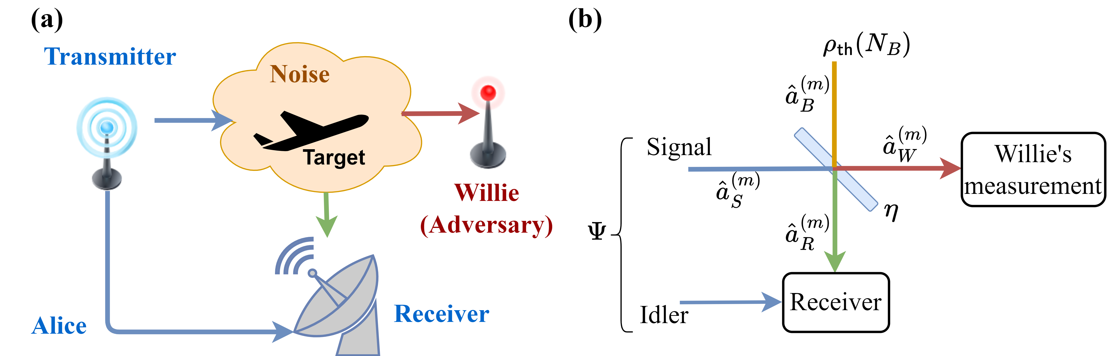
Figure 1: (a) A general covert sensing scenario: Alice (A) attempts to detect the presence of the adversary Willie (W) using an ancilla-entangled probe while remaining undetected herself. (b) Beam-splitter model: A joint state $\Psi$ with $M$ signal ($S$) and idler modes ($I$) is prepared. Each signal mode $\hat{a}_{S}^{(m)}$ is either replaced by a background mode $\hat{a}_{B}^{(m)}$ when Willie is absent, or mixed with the background at a beam splitter with reflectance $\eta\ll 1$ representing the target. Alice makes an optimal measurement on the return modes $\left\{\hat{a}_{R}^{(m)}\right\}_{m=1}^{M}$ along with the idler system. Willie, when present, makes an optimal measurement on all his modes $\left\{\hat{a}_{W}^{(m)}\right\}_{m=1}^{M}$.

In this paper, we study covert target detection with Alice using general ancilla-entangled probes. Willie – who is assumed to be present when the target is – collect all the light that is not reflected back to Alice. In contrast to a previous model of covert target detection [15], we argue that Willie – being bathed in thermal radiation coming from all directions – receives a thermal state with the same brightness as the background when Alice is absent. This is especially true in the microwave regime for which the dominant noise contribution is from the black-body background. Therefore, her sending any state (including the vacuum) in the modes that she controls that does not reduce to the same thermal state leads to a nontrivial probability of her being detected. On the other hand, Alice’s sending a state that does mimic the thermal background state for Willie’s modes permits her to have a nontrivial probability of detecting Willie while remaining perfectly undetectable herself, leading to a complicated tradeoff between their performances.

We take an operational approach and assume that Alice fixes an acceptable covertness level $\epsilon$ at the start of the protocol, where $\epsilon$-covertness is obtained whenever Willie’s optimal error probability of discerning Alice’s presence is greater than or equal to $1/2-\epsilon$ . We then show that an $\epsilon$-covert Alice is constrained to probes whose energy lies in a specified range depending on the number of modes $M$ in the probe. We develop a necessary condition that Alice’s probe must satisfy to be $\epsilon-$covert and use it to obtain a closed-form lower bound on an $\epsilon$-covert Alice’s error probability as a function only of $\epsilon$, $M$ and the loss and noise in the system. We compare this quantum limit of Alice’s error probability to the performance of TMSV probes and Gaussian-distributed coherent states as a classical benchmark. Along the way, we also obtain a universal lower bound on the error probability of distinguishing any two thermal loss channels using ancilla entanglement, of which non-adversarial QI is a special case.

Problem Setup— A covert target detection scenario is illustrated in Fig. 1. The transmitter Alice ($A$), who is assumed to also control the receiving apparatus prepares a state (called the probe)

$$\left|\psi\right\rangle_{IS}=\sum_{\mathbf{n}}\sqrt{p}_{\mathbf{n}}\left|{\chi_{\mathbf{n}}}\right\rangle_{I}\left|{\mathbf{n}}\right\rangle_{S},$$ (1)

where $\left|{\mathbf{n}}\right\rangle_{S}=\left|{n_{1}}\right\rangle_{1}\left|{n_{2}}\right\rangle_{2}\cdots\left|{n_{M}}\right\rangle_{M}$ is an $M$-mode number state of the signal ($S$) system, $\{\left|{\chi_{\mathbf{n}}}\right\rangle_{I}\}$ are normalized (not necessarily orthogonal) states of an idler ($I$) system, and $p_{\mathbf{n}}$ is the probability mass function (pmf) of $\mathbf{n}$. The signal modes are sent to probe the target region, while the $I$ system is held losslessly. The annihilation operator of the $m$-th mode $\{\hat{a}_{R}^{(m)}\}_{m=1}^{M}$ returning to Alice is

$$\hat{a}_{R}^{(m)}=\sqrt{\eta^{(h)}}\,\hat{a}_{S}^{(m)}+\sqrt{1-\eta^{(h)}}\,\hat{a}_{B}^{(m)},$$ (2)

where $\hat{a}^{(m)}_{S}$ and $\hat{a}_{B}^{(m)}$ are annihilation operators of the corresponding signal and background modes (see Fig. 1). Here $h=0$ denotes the absence of the target in which case $\eta^{(0)}=0$ while $h=1$ denotes target presence, for which $\eta^{(1)}:=\eta\ll 1$ . The adversary, Willie ($W$) is assumed to receive the output modes $\left\{\hat{a}_{W}^{(m)}\right\}_{m=1}^{M}$ from the other output of the beam splitter so that

$$\hat{a}_{W}^{(m)}=\sqrt{1-\eta}\,\hat{a}_{S}^{(m)}-\sqrt{\eta}\,\hat{a}_{B}^{(m)}.$$ (3)

We assume that under both hypotheses, each background mode $\hat{a}_{B}^{(m)}$ is in the thermal state $\rho_{\textsf{th}}\left(N_{B}\right)=\sum_{n=0}^{\infty}N_{B}^{n}/(N_{B}+1)^{n+1}\left|{n}\right\rangle\langle{n}|$. This differs from the so-called no-passive-signature (NPS) assumption made in most previous work on QI, in which the background brightness is adjusted from its nominal value $N_{B}$ to the value $N_{B}/\left(1-\eta\right)$ when the target is present. This expedient ensures that when a vacuum probe (hence “passive”) is transmitted, the returned state is the same whether or not the target is present (hence “no signature”). On the other hand, in the natural passive signature (PS) model above, sending an $M$-mode vacuum probe makes the hypotheses more distinguishable as $M$ increases. Indeed, there are several examples of quantum sensing and discrimination protocols in which the mode number $M$ is an important resource aiding the performance even when vacuum probes are used [18, 19, 20, 21]. Since $M\gg 1$ is also a prerequisite for obtaining quantum advantage in NPS QI [1, 22], comparing the PS and NPS models’ performance in this regime is warranted – this point has also been raised recently in ref. [23].

In our PS model, Alice faces the hypothesis test

$$\mathrm{H}_{0}:\;\rho_{0} =\left(\operatorname{Tr\,}_{S}\Psi\right)\otimes{\rho_{\textsf{th}}\left(N_{B}\right)}^{\otimes M},$$ (4)

$$\mathrm{H}_{1}:\;\rho_{1} =\left(\mathrm{id}_{I}\otimes\mathcal{L}_{\eta,N_{B}}^{\otimes M}\right)\Psi,$$

where $\mathcal{L}_{\kappa,N}$ denotes a thermal loss (or noisy attenuator) channel of transmittance $\kappa$ and excess noise $N_{B}$ [24] and $\Psi=\left|{\psi}\right\rangle\langle{\psi}|_{IS}$. Willie, on the other hand, faces the hypothesis test

$$\mathrm{H}_{0}^{\prime}:\;\sigma_{0} ={\rho_{\textsf{th}}\left(N_{B}\right)}^{\otimes M},$$ (5)

$$\mathrm{H}_{1}^{\prime}:\;\sigma_{1} =\mathcal{L}_{1-\eta,N_{B}}^{\otimes M}\left(\operatorname{Tr\,}_{I}\Psi\right).$$

The above tests differ from the previous study [15] of covert target detection, which invokes an NPS assumption for Alice. Concomitantly, when Willie is present, the channel between $S$ and $R$ is $\mathcal{L}_{\eta,N_{B}/\left(1-\eta\right)}$ in each mode and between $S$ and $W$ is $\mathcal{L}_{1-\eta,N_{B}/\left(1-\eta\right)}$ in each mode with $\sigma_{0}=\mathcal{L}_{1-\eta,N_{B}/\left(1-\eta\right)}^{\otimes M}\left(\left|{0}\right\rangle\left\langle 0\right|_{S}^{\otimes M}\right)=\rho_{\textsf{th}}\left(\eta N_{B}/\left(1-\eta\right)\right)^{\otimes M}$. Both parties are assumed to make optimal quantum measurements whose average error probabilities are given by the Helstrom formula [25]:

$$P_{\mathfrak{e}}^{A} =1/2-\left\|\rho_{0}-\rho_{1}\right\|_{1}/4\leq\inf_{0\leq s\leq 1}\operatorname{Tr\,}\rho_{0}^{s}\rho_{1}^{1-s}/2,$$ (6)

$$P_{\mathfrak{e}}^{W} =1/2-\left\|\sigma_{0}-\sigma_{1}\right\|_{1}/4\leq\inf_{0\leq s\leq 1}\operatorname{Tr\,}\sigma_{0}^{s}\sigma_{1}^{1-s}/2,$$ (7)

where we have assumed equal prior probabilities for simplicity and $\left\|X\right\|_{1}:=\operatorname{Tr\,}\sqrt{X^{\dagger}X}$ is the trace norm. We have also indicated the quantum Chernoff bound [26] (QCB) that is an exponentially tight upper bound on the average error probability that is often easier to calculate. The bound for $s=1/2$ is called the quantum Bhattacharyya bound. Note that, as in previous work on covert sensing and detection, two strong assumptions on Willie’s capability have been made to ensure quantum-secure performance: he is assumed to collect all the light that doesn’t return to Alice and also to know the probe that Alice would use so that he can design the best detector for his hypothesis test of Eq. (5).

For $0\leq\epsilon\leq 1/2$, a probe $\Psi$ is said to be $\epsilon$-covert if

$$P_{\mathfrak{e}}^{W}\geq 1/2-\epsilon.$$ (8)

We take an operational approach and assume that Alice has some number $M$ of signal modes available and that she fixes a covertness level $\epsilon$ acceptable to her at the start of the protocol. She then prepares the probe that minimizes $P_{\mathfrak{e}}^{A}$ over all $\epsilon-$covert probes of $M$ signal modes.

Perfect covertness— Consider the scenario of Alice sending $M$ signal modes in the limit of perfect covertness, i.e., $\epsilon=0$. This implies that $\sigma_{1}=\sigma_{0}=\rho_{\textsf{th}}\left(N_{B}\right)^{\otimes M}$. Among quantum probes, the $M$-mode TMSV state of brightness $N_{B}$ is the only pure state (modulo unitary transformations on the idler alone) that can achieve perfect covertness. Alternatively, Alice can generate coherent states in each signal mode with amplitude $\alpha\in\mathbb{C}$ chosen according to the circular Gaussian distribution $P\left(\alpha\right)=\exp\left(-\left|\alpha\right|^{2}/N_{B}\right)/\left(\pi N_{B}\right)$ to achieve $\epsilon=0$ classically – we call this a Gaussian-distributed coherent state (GCS) probe. Note that, in this case, her measurement can be conditioned on her knowledge of the amplitude transmitted in each of the $M$ shots. To compare their target detection performance, we calculate the quantum Chernoff exponents $\chi:=-\lim_{M\rightarrow\infty}\frac{\ln P_{\mathfrak{e}}^{A}}{M}$, where $P_{\mathfrak{e}}^{A}$ is Alice’s optimal error probability on an $M$-shot basis in each scenario – see Appendix A. These are very close to the quantum Bhattacharyya $(s=1/2)$ exponents, which have the approximate forms:

$$\chi_{\mathrm{TMSV}} \simeq\ln\left[1-\frac{\eta}{4}\left[1-\frac{1}{(2N_{B}+1)^{2}}\right]\right],$$ (9)

$$\chi_{\mathrm{GCS}} \simeq\ln\left[1-2\eta N_{B}\left(N_{B}-\sqrt{N_{B}(N_{B}+1)}+1\right)\right].$$

The results are compared in Fig. 2. We note that $\chi_{\mathrm{TMSV}}\geq\chi_{\mathrm{GCS}}$ everywhere with a maximum ratio of $\simeq 1.45$ around $N_{B}\simeq 0.2$ but the exponents converge in the regimes of small and large $N_{B}$.

Lower bound on Alice’s error probability— Before discussing covert detection with $\epsilon>0$, we obtain a general lower bound on Alice’s error probability as a function of the pmf $\left\{p_{n}=\sum_{\mathbf{n}:n_{1}+\cdots+n_{M}=n}p_{\mathbf{n}}\right\}_{n=0}^{\infty}$ of the total photon number of the probe (Cf. Eq. (1)). We show (Appendix B) a more general result: For $\textsf{b}\in\left\{0,1\right\}$, let states $\rho_{\textsf{b}}:=\left(\mathrm{id}_{I}\otimes\mathcal{L}_{\kappa_{\textsf{b}},N_{\textsf{b}}}^{\otimes M}\right)\Psi$ be the respective output states in response to the input $\Psi$ of any two thermal loss channels $\mathcal{L}_{\kappa_{0},N_{0}}$ and $\mathcal{L}_{\kappa_{1},N_{1}}$. Then the output fidelity $F:=\operatorname{Tr\,}\sqrt{\sqrt{\rho_{0}}\rho_{1}\sqrt{\rho_{0}}}$ satisfies

$$F\geq\nu^{M}\sum_{n=0}^{\infty}p_{n}\left[\nu\sqrt{\widetilde{\kappa}_{0}\widetilde{\kappa}_{1}}+\sqrt{\left(1-\widetilde{\kappa}_{0}\right)\left(1-\widetilde{\kappa}_{1}\right)}\right]^{n},$$ (10)

where $\nu=\left(\sqrt{G_{0}G_{1}}-\sqrt{\left(G_{0}-1\right)\left(G_{1}-1\right)}\right)^{-1}$ and $\widetilde{\kappa}_{\textsf{b}}=\kappa_{\textsf{b}}/G_{\textsf{b}}$ for $G_{\textsf{b}}=\left(1-\kappa_{\textsf{b}}\right)N_{\textsf{b}}+1$. For the target detection problem at hand, we set $\kappa_{0}=0,\kappa_{1}=\eta,N_{0}=N_{1}=N_{B}$ and use one side of the Fuchs-van de Graaf inequality [27] to conclude that

$$P_{\mathfrak{e}}^{A} \geq\frac{1}{2}\left[1-\sqrt{1-\nu^{2M}\left[\sum_{n=0}^{\infty}p_{n}\left(1-\frac{\eta}{(1-\eta)N_{B}+1}\right)^{\frac{n}{2}}\right]^{2}}\right]$$

$$\geq\frac{1}{2}\left[1-\sqrt{1-\nu^{2M}\left(1-\frac{\eta}{(1-\eta)N_{B}+1}\right)^{\mathcal{N}_{S}}}\right],$$ (11)

where $\mathcal{N}_{S}:=\sum_{n=0}^{\infty}np_{n}$ is the total signal energy and we have used Jensen’s inequality in the last step. These results may be contrasted with the lower bounds in Eqs. (12)-(13) of ref. [22] derived for NPS QI which do not display the $M$-dependent factor $\nu^{2M}$ characterizing the passive signature; Eqs. (Quantum limits of covert target detection) imply the NPS QI results if we set $N_{1}=N_{B}/(1-\eta)$.

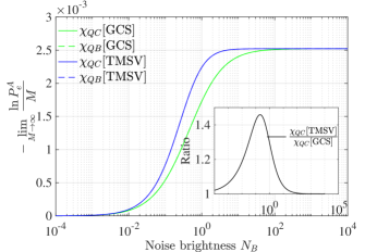
Figure 2: The quantum Chernoff (QC) (solid) and quantum Bhattacharyya (QB) (dashed) error probability exponents as a function of the noise brightness $N_{B}$ with $\eta=0.01$ for perfectly covert TMSV (blue) and GCS (green) probes. The inset shows the ratio of the exponents for the TMSV and GCS probes, which is maximized for $N_{B}\simeq 0.2$.

Necessary condition for $\epsilon$-covertness— In order to characterize $\epsilon$-covert probes for $\epsilon>0$, we formulate a necessary condition for $\epsilon$-covertness. Suppose that Alice transmits the probe $\Psi$ of Eq. (1). The Fuchs-van de Graaf inequality $P_{\mathfrak{e}}^{W}\leq F\left(\sigma_{0},\sigma_{1}\right)/2$ that relates the trace distance to the fidelity [27] between Willie’s hypothesis states (5) implies that $F\left(\sigma_{0},\sigma_{1}\right)\geq 1-2\epsilon$ is a necessary condition for $\epsilon-$covertness. In Appendix C, we use this to show that

$$\sum_{n=0}^{\infty}\sqrt{q_{n}}\sqrt{\binom{n+M-1}{n}\frac{N_{B}^{n}}{(N_{B}+1)^{n+M}}}\geq 1-2\epsilon$$ (12)

is a necessary condition for $\epsilon-$covertness, where $q_{\mathbf{n}}=\langle{\mathbf{n}}|\sigma_{1}\left|{\mathbf{n}}\right\rangle_{W}$ and $\left\{q_{n}=\sum_{\mathbf{n}:n_{1}+\cdots+n_{M}}q_{\mathbf{n}}\right\}_{n=0}^{\infty}$ is the pmf of the total photon number seen by Willie under $\mathrm{H}^{\prime}_{1}$.

Bounds on transmitter energy under $\epsilon$-covertness— We saw earlier that maintaining perfect covertness using an $M$-mode quantum or classical probe requires an energy expenditure of $MN_{B}$ photons. For $\epsilon>0$, we use Lagrange multipliers to extremize the average energy $\sum_{n=0}^{\infty}nq_{n}$ of $\sigma_{1}$ under the constraint of Eq. (73). Eq. (3) then implies that the corresponding probe energy $\mathcal{N}_{S}=\left[\sum_{n=0}nq_{n}-\eta N_{B}\right]/(1-\eta)$. We find (Fig. 3) that the probe energy must lie in a bounded region around $MN_{B}$ that gets smaller as $\epsilon$ is reduced – see Appendix D for details. We were unable to obtain an expression for the bounds on $\mathcal{N}_{S}$ as a function of the system parameters, but curve fitting indicates that the per-mode probe energy $N_{S}:=\mathcal{N}_{S}/M$ varies between $\sim N_{B}\pm A_{\pm}/\sqrt{M}$, where the $A_{\pm}$ depend only on $\eta,N_{B}$ and $\epsilon$ (See Fig. 3).

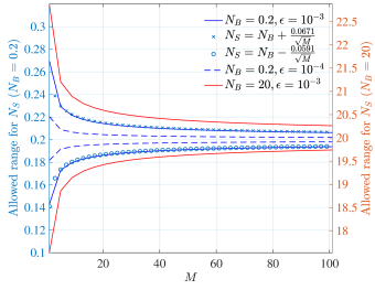
Figure 3: The maximum and minimum allowed per-mode energy $N_{S}$ for an $\epsilon$-covert probe according to Eq. (73) as a function of $M$ with $N_{B}=0.2$ and $\epsilon=10^{-3}$ (solid blue) and $\epsilon=10^{-4}$ (dashed blue). Curve fitting produced the estimates $N_{B}+0.0671/\sqrt{M}$ and $N_{B}-0.0591/\sqrt{M}$ for the maximum and minimum energy curves for $\epsilon=10^{-3}$. The allowed range of $N_{S}$ for $N_{B}=20,\epsilon=10^{-3}$ is also shown (red). $\eta=0.01$ for all curves.

Fundamental limit on Alice’s error probability under $\epsilon$-covertness— The thermal loss channel $\mathcal{L}_{1-\eta,N_{B}}$ connecting the modes in $S$ to those in $W$ (cf. Eq. (5)) admits the decomposition

$$\mathcal{L}_{1-\eta,N_{B}}=\mathcal{A}_{G}\circ\mathcal{L}_{(1-\eta)/G}$$ (13)

into a quantum-limited amplifier $\mathcal{A}_{G}$ of gain $G=\eta N_{B}+1$ and a pure-loss channel $\mathcal{L}_{(1-\eta)/G}$ of transmittance $(1-\eta)/G$ [28]. The right-hand side of the bound of Eq. (Quantum limits of covert target detection) is expressed in terms of the probability generating function (pgf) $\mathcal{P}_{S}\left(\xi\right)$ of the total photon number in $S$, defined as $\mathcal{P}_{S}\left(\xi\right):=\sum_{n=0}^{\infty}p_{n}\,\xi^{n}$ evaluated at $\xi=\sqrt{1-\eta/\left[\left(1-\eta\right)N_{B}+1\right]}$. In Appendix E, we use the decomposition (13) and develop pgf transformation techniques to find the one-to-one mapping between the photon number pgf of the probe and the pgf $\mathcal{P}_{W}\left(\xi\right):=\sum_{n=0}^{\infty}q_{n}\xi^{n}$ of the total photon number in Willie’s modes under $\mathrm{H}^{\prime}_{1}$. By connecting $\mathcal{P}_{W}\left(\xi\right)$ to the covertness condition of Eq. (73), we can show that $\epsilon-$covertness implies

$$P_{\mathfrak{e}}^{A}\geq\frac{1-\sqrt{1-\left(1-2\epsilon\right)^{4}f\left(\eta,N_{B},M\right)}}{2},$$ (14)

where the explicit expression for $f\left(\eta,N_{B},M\right)$ and the derivation of the above inequality can be found in Appendix F. Eq. (14) constitutes a probe-independent bound for $P_{\mathfrak{e}}^{A}$ given $\epsilon$-covertness.

Figure LABEL:fig:PeAcomp compares the lower bound of Eq. (14) to the performance of iid TMSV and GCS states. For each $M$, the energy of the TMSV states (as well as the average energy of the GCS states) was chosen to be the maximum allowable by the covertness constraint – see Appendix F for details. For $N_{B}=0.2$, the large-$M$ error exponent achieved by TMSV probes was about a factor of 1.37 lower than that of the bound, with the discrepancy becoming smaller for smaller $N_{B}$, along with the gap between the GCS and TMSV exponents. For larger $N_{B}$, the performance of both probes is comparable, as suggested by Fig. 2 for $\epsilon=0$, and also deviates from the lower bound.

Discussion— We have analyzed covert QI target detection in the natural passive signature (PS) model, with our lower bound (14) giving a fundamental limit on an $\epsilon$-covert Alice’s performance as a function of the number of signal modes $M$ of her probe. The maximum quantum advantage under $\epsilon-$ covertness appears to be modest and in a different range than the $N_{S}\ll 1,N_{B}\gg 1$ regime for NPS QI. It would be interesting to explore alternative models of covert detection in which Willie is limited by practical constraints, e.g., models in which he can collect only a fraction of the light not reaching Alice. The novel techniques developed here for obtaining performance bounds under $\epsilon-$covertness are likely to stimulate more research on other covert sensing protocols such as phase and transmittance sensing  [11, 12, 13]. Beyond covert sensing schemes, our fidelity bounds of Eqs. (10) on the outputs of thermal loss channels may – besides illuminating the fundamental limits of PS QI [23] – be useful for the study of schemes such as quantum reading [29], pattern recognition [30] and channel position finding [31, 32].

Acknowledgements— This work is supported by the Singapore Ministry of Education Tier 2 Grant No. T2EP50221-0014, the Singapore Ministry of Education Tier1 Grants RG146/20 and RG77/22, the Agency for Science, Technology and Research (A*STAR) under its QEP2.0 programme (NRF2021-QEP2-02-P06), and FQxI under grant no  FQXi-RFP-IPW-1903 (“Are quantum agents more energetically efficient at making predictions?”) from the Foundational Questions Institute and Fetzer Franklin Fund (a donor-advised fund of Silicon Valley Community Foundation). Any opinions, findings and conclusions or recommendations expressed in this material are those of the author(s) and do not reflect the views of National Research Foundation or the Ministry of Education, Singapore.

I Appendices

II Appendix A: Quantum Chernoff exponents for TMSV and GCS transmitters

II.1 Gaussian state specification and the quantum Chernoff bound

In this section, we describe how the quantum Chernoff exponents for TMSV and GCS probes discussed in the main text were obtained. To this end, we recall the formalism of mean vectors and covariance matrices for multimode states. We define a vector of quadrature field operators $Q=(x_{1},\ldots,x_{M},p_{1},\cdots,p_{M})^{\operatorname{\textsf{T}}}$ of an arbitrary $M$-mode system whose components are the dimensionless operators

$$\hat{q}_{m} =\frac{\hat{a}_{m}+\hat{a}_{m}^{\dagger}}{\sqrt{2}},\qquad\hat{p}_{m}=\frac{-i(\hat{a}_{m}-\hat{a}_{m}^{\dagger})}{\sqrt{2}}.$$ (15)

These quadrature operators satisfy the commutation relations:

$$[Q,Q^{\operatorname{\textsf{T}}}] =i\Omega;\qquad\Omega=\begin{pmatrix}0&1\\ -1&0\end{pmatrix}\otimes\mathbb{1}_{M}.$$ (16)

For a given state $\rho$, we have the mean vector

$$\overline{Q} =\left\langle Q\right\rangle=\operatorname{Tr\,}(Q\hat{\rho})$$ (17)

and the (Wigner) covariance matrix $\widetilde{V}$, whose $ij$-th entry is

$$\widetilde{V}_{ij} =\frac{1}{2}\left\langle\{\Delta Q_{i},\Delta Q_{j}\}\right\rangle$$

$$=\frac{1}{2}\left\langle\{Q_{i},Q_{j}\}\right\rangle-\left\langle Q_{i}\right\rangle\left\langle Q_{j}\right\rangle,$$ (18)

where $\Delta Q_{i}=Q_{i}-\left\langle Q_{i}\right\rangle$ and $\{,\}$ is the anticommutator. For Gaussian states such as those under consideration here, the mean vector and covariance matrix fully determine the state.

We recall the quantum Chernoff bound (QCB) that provides an exponentially tight upper bound on the optimal error probability for Alice’s discrimination of her hypotheses $H_{0}$ and $H_{1}$ [26]. For a priori equally likely hypotheses, it reads

$$P_{E}^{A}\left[\rho_{0},\rho_{1}\right]\leq\frac{1}{2}\left(\inf_{0\leq s\leq 1}\operatorname{Tr\,}\rho_{0}^{s}\rho_{1}^{1-s}\right)\equiv\frac{1}{2}\left(\inf_{0\leq s\leq 1}C_{s}\right).$$ (19)

Note that the QCB is multiplicative in the sense that if $\rho_{0}=\otimes_{m=1}^{M}r_{0,m}$ and $\rho_{1}=\otimes_{m=1}^{M}r_{1,m}$, we have

$$P_{E}^{A}\left[\rho_{0},\rho_{1}\right]\leq\frac{1}{2}\left(\inf_{0\leq s\leq 1}\operatorname{Tr\,}\rho_{0}^{s}\rho_{1}^{1-s}\right)=\frac{1}{2}\prod_{m=1}^{M}\left(\inf_{0\leq s\leq 1}\operatorname{Tr\,}r_{0,m}^{s}r_{1,m}^{1-s}\right).$$ (20)

Note that choosing any value of $s$ between $0$ and $1$ provides an upper bound on $P_{\mathfrak{e}}^{A}$. The case $s=1/2$ is known as the quantum Bhattacharyya bound (QBB). For Gaussian states, we can leverage exist techniques in the literature [33] to compute $C_{s}$, and thence the QCB, once the means and covariances of $\rho_{0}$ and $\rho_{1}$ are known.

II.2 Gaussian-distributed coherent-state (GCS) transmitter

As discussed in the main text, a possible classical probe that Alice can transmit consists of a string of $M$ coherent states $\left|{\alpha_{1}}\right\rangle\otimes\cdots\otimes\left|{\alpha_{M}}\right\rangle\equiv\left|{\bm{\alpha}}\right\rangle$ with amplitudes drawn independently from a circular Gaussian distribution

$$P\left(\alpha\right)=\frac{1}{\pi N_{T}}\exp\left(-\frac{\left|\alpha\right|^{2}}{N_{T}}\right),$$ (21)

where $N_{T}$ is the average per-mode transmitted energy. The reduced state seen by Willie in each signal mode is then a thermal state $\tau\left(N_{T}\right)$. Alice, on the other hand, knows the vector $\bm{\alpha}$ and can incorporate this knowledge in her receiver. Accordingly, her error probability is

$$P_{\mathfrak{e}}^{A}[\mathrm{GCS}]=\int_{\mathbb{C}^{M}}\mathop{}\!\mathrm{d}^{2M}\bm{\alpha}\,P\left(\bm{\alpha}\right)P^{A}_{E}\left[\bm{\alpha}\right],$$ (22)

where $P^{A}_{E}\left[\bm{\alpha}\right]$ is shorthand for Alice’s optimal error probability of discriminating the two possible received states when the transmitter is $\left|{\bm{\alpha}}\right\rangle$.

For a single mode in which coherent state $\left|{\alpha}\right\rangle\equiv\left|{\alpha_{r}+i\alpha_{i}}\right\rangle$ is transmitted, the mean vector and covariance matrix of the received state of $\hat{a}_{W}$ under the two hypotheses can be computed using Eq. (3) of the main text as follows:

$$\mathrm{H}_{0}: \,\overline{Q}=\begin{bmatrix}0\\ 0\end{bmatrix};\qquad\widetilde{V}=\begin{bmatrix}N_{B}+\frac{1}{2}&0\\ 0&N_{B}+\frac{1}{2}\end{bmatrix},$$ (23)

$$\mathrm{H}_{1}:\; \overline{Q}=\begin{bmatrix}\sqrt{2\eta\alpha_{r}}\\ \sqrt{2\eta\alpha_{i}}\end{bmatrix};\qquad\widetilde{V}=\begin{bmatrix}\left(1-\eta\right)N_{B}+\frac{1}{2}&0\\ 0&\left(1-\eta\right)N_{B}+\frac{1}{2}\end{bmatrix}.$$ (24)

These correspond to a thermal state and displaced thermal state respectively. The passive signature manifests in the fact that these states have slightly different temperatures.

Using the QCB Eq. (19), we can bound Alice’s error probability for an $M$-mode GCS transmitter as follows:

$$P_{\mathfrak{e}}^{A}[\mathrm{GCS}] =\int_{\mathbb{C}^{M}}\mathop{}\!\mathrm{d}^{2M}\bm{\alpha}\left(\prod_{m=1}^{M}P\left(\alpha_{m}\right)\right)P^{A}_{E}\left[\bm{\alpha}\right]$$ (25)

$$\leq\frac{1}{2}\int_{\mathbb{C}^{M}}\mathop{}\!\mathrm{d}^{2M}\bm{\alpha}\prod_{m=1}^{M}\left[P\left(\alpha_{m}\right)\left(\inf_{0\leq s\leq 1}C_{s}\left[\alpha_{m}\right]\right)\right]$$ (26)

$$=\frac{1}{2}\left[\int_{\mathbb{C}}\mathop{}\!\mathrm{d}^{2}\alpha\,P(\alpha)\left(\inf_{0\leq s\leq 1}C_{s}\left[\alpha\right]\right)\right]^{M},$$ (27)

where we have used the multiplicativity of the QCB from Eq. (20). In principle, the optimizing $s$ inside the above integral can depend on $\left|\alpha\right|$ but we found numerically that $s=1/2$ was nearly optimum for all values of $\left|\alpha\right|$ and $N_{B}$ in the $\eta\leq 0.01$ region. Accordingly, the optimal error probability exponent equals the Bhattacharyya error exponent:

$$\chi_{\mathrm{GCS}}:=-\lim_{M\rightarrow\infty}\frac{\ln\,P_{\mathfrak{e}}^{A}[\mathrm{GCS}]}{M}\simeq-\ln\int_{\mathbb{C}}\mathop{}\!\mathrm{d}^{2}\alpha\,P(\alpha)C_{1/2}\left[\alpha\right].$$ (28)

For perfect covertness, we set $N_{T}=N_{B}$ in the above and the result is approximated in Eq. (9) of the main text.

II.3 Two-mode squeezed vacuum (TMSV) transmitter

Consider using multiple copies of the TMSV state $\left|{\psi}\right\rangle=\sum_{n=0}^{\infty}\sqrt{\frac{N_{S}^{n}}{\left(N_{S}+1\right)^{n+1}}}\left|n\right\rangle_{S}\left|n\right\rangle_{I}$. This state has a zero mean vector and the covariance matrix

$$\widetilde{V}_{SI} =\begin{bmatrix}S&C\\ C&S\end{bmatrix}\oplus\begin{bmatrix}S&-C\\ -C&S\end{bmatrix},$$ (29)

where

$$S =N_{S}+\frac{1}{2},$$ (30)

$$C =\sqrt{N_{S}(N_{S}+1)},$$ (31)

and $X\oplus Y=\begin{bmatrix}X&0\\ 0&Y\end{bmatrix}$ is the direct sum of matrices.

Using Eq. (2) of the main text, we can compute the first and second moments of the states corresponding to Alice’s two hypotheses. Both states remain zero-mean, and the covariance matrices are

$$\mathrm{H}_{0}:\,\widetilde{V}_{RI} =\begin{bmatrix}B&0\\ 0&S\end{bmatrix}\oplus\begin{bmatrix}B&0\\ 0&S\end{bmatrix},$$ (32)

$$\mathrm{H}_{1}:\,\widetilde{V}_{RI} =\begin{bmatrix}A&\sqrt{\eta}C\\ \sqrt{\eta}C&S\end{bmatrix}\oplus\begin{bmatrix}A&-\sqrt{\eta}C\\ -\sqrt{\eta}C&S\end{bmatrix},$$ (33)

where

$$A =\eta N_{S}+(1-\eta)N_{B}+\frac{1}{2},$$ (34)

$$B =N_{B}+\frac{1}{2}.$$ (35)

As for the coherent-state case, the covariance matrices above can be used to numerically compute the Chernoff bounds $C_{s}$ using the techniques in Ref. [33].

III Appendix B: Lower bound for Alice’s error probability of distinguishing thermal loss channels

Among the pure-state probes $\Psi=\left|{\psi}\right\rangle\langle{\psi}|_{IS}$ with

$$\left|\psi\right\rangle_{IS} =\sum_{\mathbf{n}}\sqrt{p_{\mathbf{n}}}\left|\chi_{\mathbf{n}}\right\rangle_{I}\left|\mathbf{n}\right\rangle_{S},$$ (36)

with a given photon number pmf in $S$, the NDS probes are those satisfying $\langle{\chi_{\mathbf{n}}}|{\chi_{\mathbf{n}^{\prime}}}\rangle=\delta_{\mathbf{n},\mathbf{n}^{\prime}}$. It follows from the phase covariance of thermal loss channels and the results of ref. [34] (See Lemma 4 therein with trace distance as the divergence measure) that among all probes with a given $\{p_{\mathbf{n}}\}$, NDS transmitters have the smallest $P_{\mathfrak{e}}^{A}$. Accordingly, we can focus on them in order to derive a lower bound on $P_{\mathfrak{e}}^{A}$. For an NDS probe of the form of Eq. (36), the hypotheses to be distinguished by Alice are

$$\mathrm{H}_{0}: \rho_{0}=\left(\mathrm{id}_{I}\otimes\mathcal{L}_{0,N_{B}}^{\otimes M}\right)\Psi=\left(\mathrm{id}_{I}\otimes\left(\mathcal{A}_{G}\circ\mathcal{L}_{0}\right)^{\otimes M}\right)\Psi.$$ (37)

$$\mathrm{H}_{1}: \rho_{1}=\left(\mathrm{id}_{I}\otimes\mathcal{L}_{\kappa,N_{B}}^{\otimes M}\right)\Psi=\left(\mathrm{id}_{I}\otimes\left(\mathcal{A}_{\widetilde{G}}\circ\mathcal{L}_{\widetilde{\kappa}}\right)^{\otimes M}\right)\Psi,$$ (38)

where

$$\widetilde{G} =(1-\kappa)N_{B}+1,$$ (39)

$$\widetilde{\kappa} =\kappa/\widetilde{G}.$$ (40)

In this section, we prove the somewhat more general result of Theorem III.1. To this end, we need the following result proved in Ref. [21] (see Appendix therein).

Proposition III.1.

With $\mathbf{n}=\left(n_{1},\ldots,n_{M}\right)$ indexing the $M$-mode Fock states of $S$, consider the NDS states

$$\left|\psi\right\rangle_{IS} =\sum_{\mathbf{n}}\sqrt{r_{\mathbf{n}}}\left|\chi_{\mathbf{n}}\right\rangle_{I}\left|\mathbf{n}\right\rangle_{S},$$ (41)

$$\left|\psi^{\prime}\right\rangle_{IS} =\sum_{\mathbf{n}}\sqrt{s_{\mathbf{n}}}\left|\chi_{\mathbf{n}}\right\rangle_{I}\left|\mathbf{n}\right\rangle_{S},$$

where $\left\{r_{\mathbf{n}}\right\}$ and $\left\{s_{\mathbf{n}}\right\}$ are arbitrary multimode photon probability distributions and $\left\{\left|\chi_{\mathbf{n}}\right\rangle_{I}\right\}$ is a given orthonormal set of states in $A$. Suppose that

$$\rho =\left(\mathrm{id}_{A}\otimes\mathcal{A}_{G}^{\otimes M}\right)\left(\left|{\psi}\right\rangle\langle{\psi}|\right),$$ (42)

$$\rho^{\prime} =\left(\mathrm{id}_{A}\otimes\mathcal{A}_{G^{\prime}}^{\otimes M}\right)\left(\left|{\psi^{\prime}}\right\rangle\langle{\psi^{\prime}}|\right).$$

The fidelity between these output states is given by

$$F\left(\rho,\rho^{\prime}\right) =\sum_{\mathbf{n}\geq\mathbf{0}}\sqrt{r_{\mathbf{n}}\,s_{\mathbf{n}}}\;\nu^{n+M},$$ (43)

where $n=\sum_{m=1}^{M}n_{m}$ and

$$\nu=\left(\sqrt{GG^{\prime}}-\sqrt{\left(G-1\right)\left(G^{\prime}-1\right)}\right)^{-1}\in(0,1].$$ (44)

Theorem III.1.

Consider two cascaded channels

$$\mathcal{C} :=\left(\mathcal{A}_{G}\circ\mathcal{L}_{\kappa}\right)^{\otimes M},$$ (45)

$$\mathcal{C}^{\prime} :=\left(\mathcal{A}_{G^{\prime}}\circ\mathcal{L}_{\kappa^{\prime}}\right)^{\otimes M},$$

acting on an $M$-mode system S and an NDS probe state

$$\left|\psi\right\rangle_{IS}=\sum_{\mathbf{n}}\sqrt{p_{\mathbf{n}}}\left|\chi_{\mathbf{n}}\right\rangle_{I}\left|\mathbf{n}\right\rangle_{S}$$ (46)

and let $\Psi=\left|{\psi}\right\rangle\langle{\psi}|_{IS}$. Let

$$p_{n}=\sum_{\mathbf{n}\geq\mathbf{0}:\operatorname{tr\,}\mathbf{n}=n}p_{\mathbf{n}}$$ (47)

be the probability distribution of the total photon number in $S$. For the output states

$$\rho =\left(\mathrm{id}_{I}\otimes\mathcal{C}\right)\left(\Psi\right),$$ (48)

$$\rho^{\prime} =\left(\mathrm{id}_{I}\otimes\mathcal{C}^{\prime}\right)\left(\Psi\right),$$

we have the lower bound

$$F\left(\rho,\rho^{\prime}\right)\geq\nu^{M}\sum_{n=0}^{\infty}p_{n}\left[\nu\sqrt{\kappa\kappa^{\prime}}+\sqrt{\left(1-\kappa\right)\left(1-\kappa^{\prime}\right)}\right]^{n},$$ (49)

on the fidelity between them, where $\nu$ is given by Eq. (44).

Proof.

Consider the states

$$\sigma =\left(\mathrm{id}_{A}\otimes\mathcal{L}_{\kappa}^{\otimes M}\right)\left(\Psi\right),$$ (50)

$$\sigma^{\prime} =\left(\mathrm{id}_{A}\otimes\mathcal{L}_{\kappa^{\prime}}^{\otimes M}\right)\left(\Psi\right).$$

Let $\kappa=\cos^{2}\phi$ and $\kappa^{\prime}=\cos^{2}\phi^{\prime}$. The states above can be written as a mixture of states corresponding to the ‘loss pattern’ $\mathbf{l}$ of photons to the environment of the attenuator as [35]:

$$\sigma =\sum_{\mathbf{l}\geq\mathbf{0}}\left|{\psi_{\mathbf{l}}}\right\rrangle\left\llangle\psi_{\mathbf{l}}\right|\equiv\sum_{\mathbf{l}\geq\mathbf{0}}q_{\mathbf{l}}\,\left|{\psi_{\mathbf{l}}}\right\rangle\langle{\psi_{\mathbf{l}}}|\equiv\sum_{\mathbf{l}\geq\mathbf{0}}q_{\mathbf{l}}\Psi_{\mathbf{l}},$$ (51)

$$\sigma^{\prime} =\sum_{\mathbf{l}\geq\mathbf{0}}\left|{\psi^{\prime}_{\mathbf{l}}}\right\rrangle\left\llangle\psi^{\prime}_{\mathbf{l}}\right|\equiv\sum_{\mathbf{l}\geq\mathbf{0}}q^{\prime}_{\mathbf{l}}\,\left|{\psi^{\prime}_{\mathbf{l}}}\right\rangle\langle{\psi^{\prime}_{\mathbf{l}}}|\equiv\sum_{\mathbf{l}\geq\mathbf{0}}q^{\prime}_{\mathbf{l}}\Psi^{\prime}_{\mathbf{l}},$$

with

$$\left|{\psi_{\mathbf{l}}}\right\rrangle =\left[\sin\phi\right]^{\operatorname{tr\,}\mathbf{l}}\sum_{\mathbf{n}\geq\mathbf{l}}\sqrt{p_{\mathbf{n}}}\left[\cos\phi\right]^{\operatorname{tr\,}\mathbf{n}-\operatorname{tr\,}\mathbf{l}}\sqrt{\prod_{m=1}^{M}{n_{m}\choose l_{m}}}\left|\chi_{\mathbf{n}}\right\rangle_{I}\left|\mathbf{n}-\mathbf{l}\right\rangle_{S}$$ (52)

$$=\left[\sin\phi\right]^{\operatorname{tr\,}\mathbf{l}}\sum_{\mathbf{n}\geq\mathbf{0}}\sqrt{p_{\mathbf{n}+\mathbf{l}}}\left[\cos\phi\right]^{\operatorname{tr\,}\mathbf{n}}\sqrt{\prod_{m=1}^{M}{n_{m}+l_{m}\choose l_{m}}}\left|\chi_{\mathbf{n}+\mathbf{l}}\right\rangle_{I}\left|\mathbf{n}\right\rangle_{S}$$

$$\equiv\sum_{\mathbf{n}\geq\mathbf{0}}\sqrt{r_{\mathbf{n}}^{(\mathbf{l})}}\left|\xi^{(\mathbf{l})}_{\mathbf{n}}\right\rangle_{I}\left|\mathbf{n}\right\rangle_{S}$$

$$\equiv\sqrt{q_{\mathbf{l}}}\left|{\psi_{\mathbf{l}}}\right\rangle$$

an NDS state with squared norm $q_{\mathbf{l}}=\langle{\psi_{\mathbf{l}}}|{\psi_{\mathbf{l}}}\rangle$. Similarly,

$$\left|{\psi^{\prime}_{\mathbf{l}}}\right\rrangle =\left[\sin\phi^{\prime}\right]^{\operatorname{tr\,}\mathbf{l}}\sum_{\mathbf{n}\geq\mathbf{l}}\sqrt{p_{\mathbf{n}}}\left[\cos\phi^{\prime}\right]^{\operatorname{tr\,}\mathbf{n}-\operatorname{tr\,}\mathbf{l}}\sqrt{\prod_{m=1}^{M}{n_{m}\choose l_{m}}}\left|\chi_{\mathbf{n}}\right\rangle_{I}\left|\mathbf{n}-\mathbf{l}\right\rangle_{S}$$ (53)

$$=\left[\sin\phi^{\prime}\right]^{\operatorname{tr\,}\mathbf{l}}\sum_{\mathbf{n}\geq\mathbf{0}}\sqrt{p_{\mathbf{n}+\mathbf{l}}}\left[\cos\phi^{\prime}\right]^{\operatorname{tr\,}\mathbf{n}}\sqrt{\prod_{m=1}^{M}{n_{m}+l_{m}\choose l_{m}}}\left|\chi_{\mathbf{n}+\mathbf{l}}\right\rangle_{I}\left|\mathbf{n}\right\rangle_{S}$$

$$\equiv\sum_{\mathbf{n}\geq\mathbf{0}}\sqrt{{r^{\prime}}_{\mathbf{n}}^{(\mathbf{l})}}\left|\xi^{(\mathbf{l})}_{\mathbf{n}}\right\rangle_{I}\left|\mathbf{n}\right\rangle_{S}$$

$$\equiv\sqrt{q^{\prime}_{\mathbf{l}}}\left|{\psi^{\prime}_{\mathbf{l}}}\right\rangle$$

an NDS state with squared norm $q^{\prime}_{\mathbf{l}}=\langle{\psi^{\prime}_{\mathbf{l}}}|{\psi^{\prime}_{\mathbf{l}}}\rangle$.

Since

$$\rho =\left(\mathrm{id}_{A}\otimes\mathcal{A}_{G}^{\otimes M}\right)\left(\sigma\right),$$ (54)

$$\rho^{\prime} =\left(\mathrm{id}_{A}\otimes\mathcal{A}_{G^{\prime}}^{\otimes M}\right)\left(\sigma^{\prime}\right),$$

we can use the strong concavity of fidelity [36] to write

$$F\left(\rho,\rho^{\prime}\right) \geq\sum_{\mathbf{l}\geq\mathbf{0}}\sqrt{q_{\mathbf{l}}\,q^{\prime}_{\mathbf{l}}}\;F\left(\mathrm{id}_{A}\otimes\mathcal{A}_{G}^{\otimes M}\left(\Psi_{\mathbf{l}}\right),\mathrm{id}_{A}\otimes\mathcal{A}_{G^{\prime}}^{\otimes M}\left(\Psi^{\prime}_{\mathbf{l}}\right)\right).$$ (55)

We can now apply Eq. (43) from Proposition III.1 to write the summand above as $\sum_{n=0}^{\infty}f_{n}^{(\mathbf{l})}\nu^{n+M}$ where

$$f_{n}^{(\mathbf{l})}=\sum_{\mathbf{n}:\operatorname{tr\,}\mathbf{n}=n}\sqrt{{r}_{\mathbf{n}}^{(\mathbf{l})}\,{r^{\prime}}_{\mathbf{n}}^{(\mathbf{l})}}.$$ (56)

The right-hand side of (55) then becomes

$$F\left(\rho,\rho^{\prime}\right) \geq\sum_{\mathbf{l}\geq\mathbf{0}}\sum_{n=0}^{\infty}\nu^{n+M}\sum_{\mathbf{n}:\operatorname{tr\,}\mathbf{n}=n}\sqrt{{r}_{\mathbf{n}}^{(\mathbf{l})}\,{r^{\prime}}_{\mathbf{n}}^{(\mathbf{l})}}$$ (57)

$$=\nu^{M}\sum_{\mathbf{l}\geq\mathbf{0}}\sum_{\mathbf{n}\geq\mathbf{0}}p_{\mathbf{n}+\mathbf{l}}\left[\sin\phi\,\sin\phi^{\prime}\right]^{\operatorname{tr\,}\mathbf{l}}\left[\nu\,\cos\phi\,\cos\phi^{\prime}\right]^{\operatorname{tr\,}\mathbf{n}}\left(\prod_{m=1}^{M}{n_{m}+l_{m}\choose l_{m}}\right)$$ (58)

Setting $\mathbf{k}=\mathbf{n}+\mathbf{l}$, the sum can be rewritten as

$$F\left(\rho,\rho^{\prime}\right) \geq\nu^{M}\sum_{\mathbf{k}\geq\mathbf{0}}p_{\mathbf{k}}\left[\nu\cos\phi\cos\phi^{\prime}\right]^{\operatorname{tr\,}\mathbf{k}}\sum_{\mathbf{l}\leq\mathbf{k}}\left[\nu^{-1}\tan\phi\tan\phi^{\prime}\right]^{\operatorname{tr\,}\mathbf{l}}\left(\prod_{m=1}^{M}{k_{m}\choose l_{m}}\right)$$ (59)

$$=\nu^{M}\sum_{\mathbf{k}\geq\mathbf{0}}p_{\mathbf{k}}\left[\nu\cos\phi\cos\phi^{\prime}+\sin\phi\sin\phi^{\prime}\right]^{\operatorname{tr\,}\mathbf{k}}$$ (60)

$$=\nu^{M}\sum_{n=0}^{\infty}p_{n}\left[\nu\sqrt{\kappa\kappa^{\prime}}+\sqrt{(1-\kappa)(1-\kappa^{\prime})}\right]^{n}.$$ (61)

∎

Eq. (47) corresponds to Eq. (10) of the main text. This generalizes a similar result derived for quantum-limited loss channels [37] that can be recovered by setting $G^{\prime}=G=1$. A bound expressed only in terms of the total probe energy $\mathcal{N}_{S}=\sum_{n=0}^{\infty}np_{n}$ can be obtained using Jensen’s inequality.

Returning to Alice’s target detection problem, we set $\kappa=0,G=N_{B}+1,\kappa^{\prime}=\eta/G^{\prime},G^{\prime}=(1-\eta)N_{B}+1$ to get the lower bound

$$F\left(\rho_{0},\rho_{1}\right)\geq\nu^{M}\sum_{n=0}^{\infty}p_{n}\left(1-\frac{\kappa}{(1-\kappa)N_{B}+1}\right)^{n/2},$$ (62)

which in turn implies via the results of [27] that

$$P_{\mathfrak{e}}^{A}\geq\frac{1-\sqrt{1-F^{2}\left(\rho_{0},\rho_{1}\right)}}{2},$$ (63)

which leads to Eq. (11) of the main text.

IV Appendix C: Necessary condition for $\epsilon$-covertness

In this section, we derive a necessary condition for $\epsilon$-covertness. The condition applies to any $M$-signal-mode probe and is expressed in terms of the photon number probability mass function (pmf) of the total photon number in the state $\sigma_{1}$ of Eq. (5) corresponding to Willie’s alternative hypothesis $\mathrm{H}_{1}^{\prime}$.

Willie’s null hypothesis state is

$$\sigma_{0} =\tau\left(N_{B}\right)^{\otimes M}=\prod_{m=1}^{M}\left[\sum_{n_{m}=0}^{\infty}\frac{N_{B}^{n_{m}}}{\left(N_{B}+1\right)^{n_{m}+1}}\left|{n_{m}}\right\rangle\langle{n_{m}}|\right],$$ (64)

$$=\sum_{\mathbf{n}\geq\mathbf{0}}\frac{N_{B}^{n}}{\left(N_{B}+1\right)^{n+M}}\left|{\mathbf{n}}\right\rangle\langle{\mathbf{n}}|,$$ (65)

where $\left|{\mathbf{n}}\right\rangle_{W}=\left|{n_{1}}\right\rangle\otimes\cdots\otimes\left|{n_{M}}\right\rangle$ are $M$-mode number states of Willie’s modes and we have defined the total photon number $n:=\operatorname{tr\,}\mathbf{n}=\sum_{m=1}^{M}n_{m}$. A general alternative-hypothesis state can be written as

$$\sigma_{1}=\sum_{\mathbf{n},\mathbf{n}^{\prime}\geq\mathbf{0}}q_{\textbf{n},\textbf{n}^{\prime}}\left|{\textbf{n}}\right\rangle\langle{\textbf{n}^{\prime}}|.$$ (66)

The $\epsilon$-covertness condition (Eq. (8) of the main text) reads

$$\frac{1}{2}-\epsilon\leq P_{\mathfrak{e}}^{W}=\frac{1}{2}-\frac{\left\|\sigma_{0}-\sigma_{1}\right\|_{1}}{4}\leq\frac{F\left(\sigma_{0},\sigma_{1}\right)}{2},$$ (67)

where $F\left(\sigma_{0},\sigma_{1}\right)=\operatorname{Tr\,}\sqrt{\sqrt{\sigma_{0}}\sigma_{1}\sqrt{\sigma_{0}}}$ is the fidelity between $\sigma_{0}$ and $\sigma_{1}$ and the last inequality is due to Fuchs and van de Graaf [27].

Let $\mathcal{M}$ be the channel correponding to a (non-destructive) measurement of photon number in each of Willie’s modes, i.e, $\mathcal{M}\sigma=\sum_{\mathbf{n}\geq\mathbf{0}}\langle{\mathbf{n}}|\sigma\left|{\mathbf{n}}\right\rangle\left|{\mathbf{n}}\right\rangle\langle{\mathbf{n}}|$ for any input state $\sigma$. Using the data processing inequality for the fidelity, we can write

$$F\left(\sigma_{0},\sigma_{1}\right) \leq F\left(\mathcal{M}\sigma_{0},\mathcal{M}\sigma_{1}\right)$$ (68)

$$=F\left(\sigma_{0},\mathcal{M}\sigma_{1}\right)$$ (69)

$$=F\left(\sigma_{0},\sum_{\mathbf{n}}q_{\mathbf{n}}\left|{\mathbf{n}}\right\rangle\langle{\mathbf{n}}|\right)$$ (70)

$$=\sum_{n=0}^{\infty}\sqrt{\frac{N_{B}^{n}}{\left(N_{B}+1\right)^{n+M}}}\left(\sum_{\mathbf{n}:\operatorname{tr\,}\mathbf{n}=n}\sqrt{q_{\mathbf{n}}}\right),$$ (71)

where we have set $q_{\mathbf{n}}:=q_{\mathbf{n},\mathbf{n}}$. This bound is complicated in that it is expressed in terms of the photon number pmf of all of Willie’s modes. To get a bound only in terms of the pmf $q_{n}=\sum_{\mathbf{n}:n_{1}+\cdots+n_{M}=n}q_{\mathbf{n}}$ of the total photon number, note that

$$\sum_{\mathbf{n}:\operatorname{tr\,}\mathbf{n}=n}\sqrt{q_{\mathbf{n}}} \leq\sqrt{q_{n}}\sqrt{\binom{n+M-1}{n}},$$ (72)

where the binomial coefficient is the number of terms in the sum on the left-hand side. This inequality is saturated if $\{q_{\mathbf{n}}\}$ is a product thermal distribution of any brightness. Substituting the above inequality into Eq. (71) and using Eq. (67), we get the necessary condition

$$\sum_{n=0}^{\infty}\sqrt{q_{n}}\sqrt{\binom{n+M-1}{n}\frac{N_{B}^{n}}{(N_{B}+1)^{n+M}}}\geq 1-2\epsilon$$ (73)

for $\epsilon$-covertness given as Eq. (12) of the main text.

V Appendix D: Range of allowed energies for an $\epsilon-$covert probe

In this section, we obtain upper and lower limits on Alice’s allowed signal energy beyond which $\epsilon$-covertness cannot hold. As discussed in the main text, this can be done by solving the problem:

$$\textbf{Extremise }f(q_{1},q_{2},\cdots)=\sum_{n=0}^{\infty}nq_{n}$$

subject to

$$\quad g(q_{1},q_{2},\cdots)=1-2\epsilon-\sum_{n=0}^{\infty}\sqrt{\binom{n+M-1}{n}\frac{N_{B}^{n}}{(N_{B}+1)^{n+M}}q_{n}}\leq 0$$

$$\quad h(q_{1},q_{2},\cdots)=\sum_{n=0}^{\infty}q_{n}-1=0$$

where $g(q_{1},q_{2},\cdots)$ is the covertness constraint (Eq. (12) of the main text) and $\{q_{n}\}$ is the pmf of Willie’s total photon number under $\mathrm{H}_{1}^{\prime}$. The Karush-Kuhn-Tucker (KKT) necessary conditions are as follows:
Stationarity
To find the point $\vec{q}^{*}$ that minimises $f(q_{1},q_{2},\cdots)$ across all discrete probability distributions $\vec{q}$, the required condition is

$$\frac{\partial}{\partial\vec{q}}\left.\left[f+\lambda_{1}(g)+\lambda_{2}(h)\right]\right|_{\vec{q}=\vec{q}^{*}}=0,$$ (74)

which gives the system of equations for $k=1,2,\cdots$ such that

$$\frac{\partial}{\partial q_{k}}\left.\left[-\sum_{n=0}^{\infty}nq_{n}+\lambda_{1}\left(1-2\epsilon-\sum_{n=0}^{\infty}\sqrt{\binom{n+M-1}{n}\frac{N_{B}^{n}}{(N_{B}+1)^{n+M}}q_{n}}\right)+\lambda_{2}\left(\sum_{n=0}^{\infty}q_{n}-1\right)\right]\right|_{q_{k}=q_{k}^{*}}=0$$

$$-k-\lambda_{1}\sqrt{\binom{n+M-1}{n}\frac{N_{B}^{n}}{(N_{B}+1)^{n+M}}}\left(\frac{1}{2\sqrt{q_{k}^{*}}}\right)+\lambda_{2}=0,$$

$$q_{k}^{*}=\frac{\lambda_{1}^{2}}{4(k-\lambda_{2})^{2}}\left[\binom{n+M-1}{n}\frac{N_{B}^{n}}{(N_{B}+1)^{n+M}}\right]$$ (75)

where $\lambda_{1}$ and $\lambda_{2}$ are the KKT multipliers.
Primal feasibility

$$\sum_{k=0}^{\infty}q_{k}^{*}-1=0\hskip 250.0pt$$ (76)

$$1-2\epsilon-\sum_{n=0}^{\infty}\sqrt{\binom{n+M-1}{n}\frac{N_{B}^{n}}{(N_{B}+1)^{n+M}}q_{k}^{*}}\leq 0$$ (77)

Dual feasibility

$$\lambda_{1}\geq 0\hskip 290.0pt$$ (78)

Complementary slackness

$$\lambda_{1}\left(1-2\epsilon-\sum_{n=0}^{\infty}\sqrt{\binom{n+M-1}{n}\frac{N_{B}^{n}}{(N_{B}+1)^{n+M}}q_{k}^{*}}\right)=0\hskip 190.0pt$$ (79)

From the stationarity condition, it can be concluded that $\lambda_{1}\neq 0$ or the normalization condition for $\{q_{n}\}$ will be violated. Hence, by applying this condition into complementary slackness condition, it can be deduced that $\sum_{n=0}^{\infty}\sqrt{\binom{n+M-1}{n}\frac{N_{B}^{n}}{(N_{B}+1)^{n+M}}q_{k}^{*}}=1-2\epsilon$. In this case, the optimal solution is on the boundary of the constraint $g(q_{1},q_{2},\cdots)$. Substituting Eq. (75) into both constraints and confining the upper summation limit to a finite value yields the following simultaneous equations

$$\sum_{n=0}^{d}\mathcal{N}\frac{\lambda_{1}^{2}}{4(n-\lambda_{2})^{2}}\left[\binom{n+M-1}{n}\frac{N_{B}^{n}}{(N_{B}+1)^{n+M}}\right]=1$$

$$\sum_{n=0}^{d}\mathcal{N}\left[\binom{n+M-1}{n}\frac{N_{B}^{n}}{(N_{B}+1)^{n+M}}\right]\left|\frac{\lambda_{1}}{2(n-\lambda_{2})}\right|=1-2\epsilon$$ (80)

where $d$ is the upper summation limit, $\mathcal{N}$ is the re-normalisation factor for finite summation. By selecting appropriate initial values for the KKT multipliers $\lambda_{1}$ and $\lambda_{2}$ in Matlab’s numerical solver, both the upper limit and lower limit of the signal strength intercepted by Wille are obtained. Given the relationship between Alice’s allowable signal energies and Willie’s intercepted energies $\mathcal{N}_{S}=(\sum_{n}nq_{n}-\eta N_{B})/(1-\eta)$, the upper and lower allowable probe energies given $\epsilon$-covertness are obtained, as displayed in Fig. 3 of the main text.

VI Appendix E: Photon-number probability generating functions (PGFs)

In this section, we show how the pmf of the total photon number in $W$ (Willie’s modes) can be connected to the pmf of the total photon number in $S$ (the transmitter). To do so, we first review the notion of the photon number probability generating function and discuss its transformation under the pure-loss and quantum-limited amplifier channels, building on the single-mode treatment in ref. [38], Ch. 9.

VI.1 Three kinds of generating functions

Let $\mathcal{H}$ be the Hilbert space of some fixed $M$-mode quantum system. Given a state $\rho\in\mathcal{S}\left(\mathcal{H}\right)$, its photon-number probability generating function (pgf) (henceforth ‘the pgf’) is the function of the $M$-vector $\bm{\xi}=\left(\xi_{1},\ldots,\xi_{M}\right)\in\mathbb{R}^{M}$ defined as

$$\mathcal{P}\left(\bm{\xi}\right):=\sum_{\mathbf{n}\geq\mathbf{0}}p_{\mathbf{n}}\prod_{m=1}^{M}\xi_{m}^{n_{m}},$$ (81)

where $p_{\mathbf{n}}=\langle{\mathbf{n}}|\rho\left|{\mathbf{n}}\right\rangle$ is the photon number pmf on the $M$ modes of the system. Eq. (81) is the straightforward multimode generalization of the single-mode definition [38]. Because of the normalization $\sum_{\mathbf{n}}p_{\mathbf{n}}=1$, the pgf is seen to exist at least for all $\bm{\xi}$ such that $\left|\xi_{m}\right|\leq 1$ for all $m$ between $1$ and $M$. The photon-number pmf can be recovered from it via

$$p_{\mathbf{n}}=\frac{\left[\partial_{1}^{n_{1}}\cdots\partial_{M}^{n_{m}}\mathcal{P}\left(\bm{\xi}\right)\right]\Big{|}_{\bm{\xi}=\mathbf{0}}}{n_{1}!\cdots n_{M}!},$$ (82)

where $\partial_{m}\equiv\partial/\partial\xi_{m}$. Moreover, it is easily checked that the pgf of the total photon number $p_{n}=\sum_{\mathbf{n}:\operatorname{tr\,}\mathbf{n}=n}p_{\mathbf{n}}$ in $S$ can be obtained from $\mathcal{P}\left(\bm{\xi}\right)$ as

$$\mathcal{P}\left(\xi\right):=\sum_{n=0}^{\infty}p_{n}\xi^{n}=\mathcal{P}\left(\xi,\ldots,\xi\right);\qquad\xi\in\mathbb{R}.$$ (83)

To avoid proliferation of notation, we use the same symbol for the multimode pgf and that of the total photon number, letting the argument specify which is meant.

Let $\mathbf{r}=\left(r_{1},\ldots,r_{M}\right)$ be a vector of nonnegative integers. The $\mathbf{r}$-th falling factorial moment of $\rho$ is defined – generalizing the single-mode definition (cf. Sec. 9.1 of ref. [38]) – as

$$F_{\mathbf{r}}:=\operatorname{Tr\,}\rho\left[\prod_{m=1}^{M}{\hat{a}_{m}}^{{\dagger}r_{m}}{\hat{a}_{m}}^{r_{m}}\right],$$ (84)

where $\{\hat{a}_{m}\}_{m=1}^{M}$ are the annihilation operators of the $M$ modes of the system. The falling-factorial moment generating function (falling-factorial mgf) is then defined as

$$\mathcal{F}\left(\bm{\xi}\right):=\sum_{\mathbf{r}\geq\mathbf{0}}F_{\mathbf{r}}\frac{\xi_{1}^{r_{1}}}{r_{1}!}\cdots\frac{\xi_{M}^{r_{M}}}{r_{M}!}.$$ (85)

We can generalize the derivation of the single-mode correspondence given in Eq. (9.4) of ref. [38] to obtain the relation

$$\mathcal{F}\left(\bm{\xi}\right)=\mathcal{P}\left(1+\xi_{1},\ldots,1+\xi_{M}\right),$$ (86)

between the falling-factorial mgf and the pgf for an $M$-mode state.

Similarly, for any $\mathbf{r}=\left(r_{1},\ldots,r_{M}\right)$, the $\mathbf{r}$-th rising factorial moment of $\rho$ is defined as

$$R_{\mathbf{r}}:=\operatorname{Tr\,}\rho\left[\prod_{m=1}^{M}{\hat{a}_{m}}^{r_{m}}{\hat{a}_{m}}^{{\dagger}r_{m}}\right].$$ (87)

The rising-factorial moment generating function (rising-factorial mgf) is then defined as

$$\mathcal{R}\left(\bm{\xi}\right):=\sum_{\mathbf{r}\geq\mathbf{0}}R_{\mathbf{r}}\frac{\xi_{1}^{r_{1}}}{r_{1}!}\cdots\frac{\xi_{M}^{r_{M}}}{r_{M}!}.$$ (88)

This object is related to the pgf of $\rho$ via

$$\mathcal{R}\left(\bm{\xi}\right) =\left[\prod_{m=1}^{M}\left(\frac{1}{1-\xi_{m}}\right)\right]\mathcal{P}\left(\frac{1}{1-\xi_{1}},\cdots,\frac{1}{1-\xi_{M}}\right),$$ (89)

which generalizes the single-mode relation given in Eq. (9.6) of ref. [38]. Thus, any of these three functions can be derived from any other.

VI.2 PGF at the output of a thermal loss channel

The falling-factorial and rising-factorial mgfs are useful because they transform in a simple manner under the action of pure-loss and quantum-limited amplifier channels respectively. For a single-mode state $\rho$, let $\rho_{\textsf{out}}=\mathcal{L}_{\kappa}\rho$, the falling-factorial mgf $\mathcal{F}_{\textsf{out}}\left(\xi\right)$ of $\rho_{\textsf{out}}$ is related to the falling-factorial mgf $\mathcal{F}\left(\xi\right)$ of $\rho$ as:

$$\mathcal{F}_{\textsf{out}}\left(\xi\right)=\mathcal{F}\left(\kappa\xi\right).$$ (90)

Similarly, if $\rho_{\textsf{out}}=\mathcal{A}_{G}\rho$, the rising-factorial mgf $\mathcal{R}_{\textsf{in}}\left(\xi\right)$ of $\rho_{\textsf{out}}$ is related to the rising-factorial mgf $\mathcal{R}\left(\xi\right)$ of $\rho$ as:

$$\mathcal{R}_{\textsf{out}}\left(\xi\right)=\mathcal{R}\left(G\xi\right);$$ (91)

see Eqs. (9.27) and (9.36) in ref. [38].

If $\rho$ is an $M$-mode state and $\rho_{\textsf{out}}=\mathcal{L}_{\kappa}^{\otimes M}\rho$, we can generalize the derivation of Eq. (90) to show that the $M$-mode falling-factorial of Eq. (85) transforms as

$$\mathcal{F}_{\textsf{out}}\left(\bm{\xi}\right)=\mathcal{F}\left(\kappa\bm{\xi}\right).$$ (92)

On the other hand, if $\rho_{\textsf{out}}=\mathcal{A}_{G}^{\otimes M}\rho$, the $M$-mode rising-factorial mgf of Eq. (88) transforms as

$$\mathcal{R}_{\textsf{out}}\left(\bm{\xi}\right)=\mathcal{R}\left(G\bm{\xi}\right).$$ (93)

Now suppose that $\mathcal{C}$ is a product thermal loss channel that has the decomposition

$$\mathcal{C}=\mathcal{A}_{G}^{\otimes M}\circ\mathcal{L}_{\kappa}^{\otimes M}.$$ (94)

By using Eqs. (92)-(93) together with the relations of Eqs. (86)-(89) relating the mgfs to the pgf, we can show that the pgf $P_{\textsf{out}}\left(\bm{\xi}\right)$ of the output state $\rho_{\textsf{out}}=\mathcal{C}\rho$ is related to the pgf $P\left(\bm{\xi}\right)$ of $\rho$ via

$$\mathcal{P}_{\textsf{out}}\left(\bm{\xi}\right) =\left[\prod_{m=1}^{M}\frac{1}{G-\xi_{m}(G-1)}\right]\,\mathcal{P}\left(1-\kappa+\frac{\kappa\xi_{1}}{G-\xi_{1}(G-1)},\ldots,1-\kappa+\frac{\kappa\xi_{M}}{G-\xi_{M}(G-1)}\right).$$ (95)

In particular, the pgf $\mathcal{P}_{\textsf{out}}(\xi)$ of the total photon number in the output of the thermal loss channel can be related to the pgf $P\left(\xi\right)$ of the total photon number in the input via Eq. (83) as:

$$\mathcal{P}_{\textsf{out}}(\xi) =\left[\frac{1}{G-\xi(G-1)}\right]^{M}\,\mathcal{P}\left(1-\kappa+\frac{\kappa\xi}{G-\xi(G-1)}\right).$$ (96)

VII Appendix F: Lower bound on Alice’s error probability under $\epsilon$-covertness

In this section, we derive the lower bound of Eq. (14) of the main text that must be satisfied under $\epsilon-$ covertness.

VII.1 Analytical bound

We begin by rewriting the $\epsilon-$ covertness condition of Eq. (12) of the main text as

$$\sum_{n=0}^{\infty}\sqrt{\binom{n+M-1}{n}\frac{N_{B}^{n}}{(N_{B}+1)^{n+M}}x^{-n}x^{n}q_{n}}\geq 1-2\epsilon,$$ (97)

where $x$ will be specified later. Using Cauchy-Schwartz inequality, the expression can be bounded as a function of the input probability generating function

$$\sum_{n=0}^{\infty}\sqrt{\binom{n+M-1}{n}\frac{N_{B}^{n}}{(N_{B}+1)^{n+M}}x^{-n}x^{n}q_{n}}\geq 1-2\epsilon$$

$$\left(\sum_{n=0}^{\infty}\binom{n+M-1}{n}\frac{N_{B}^{n}}{(N_{B}+1)^{n+M}}x^{-n}\right)^{1/2}\left(\sum_{n=0}^{\infty}q_{n}x^{n}\right)^{1/2}\geq 1-2\epsilon$$

$$\left(\frac{1}{N_{B}+1-\frac{N_{B}}{x}}\right)^{M}\mathcal{P}_{W}(x)\geq(1-2\epsilon)^{2},$$ (98)

where $\mathcal{P}_{W}(x)$ is the probability generating function of $\sigma_{1}$. For the first sum to converge, we must have $N_{B}/\left|x\right|\leq N_{B}+1$. Using Eq. (96) to express the above inequality in terms of the pgf $\mathcal{P}_{S}$ of the probe gives

$$\mathcal{P}_{S}\left(1+\frac{(x-1)(1-\eta)}{\eta N_{B}(1-x)+1}\right)\geq(1-2\epsilon)^{2}\left(N_{B}+1-\frac{N_{B}}{x}\right)^{M}\left[\eta N_{B}(1-x)+1\right]^{M}.$$ (99)

The lower bound (Eq. (11) of the main text) on $P_{\mathfrak{e}}^{A}$ for QI target detection is a function of the fidelity between $\rho_{0}$ and $\rho_{1}$, namely $P_{\mathfrak{e}}^{A}\geq 1/2-\sqrt{1-F^{2}(\rho_{0},\rho_{1})}/2$, where the fidelity is lower-bounded in terms of the probe pgf as follows:

$$F(\rho_{0},\rho_{1}) \geq\nu^{M}\sum_{n=0}^{\infty}p_{n}\left[1-\frac{\eta}{(1-\eta)N_{B}+1}\right]^{n/2}$$

$$=\nu^{M}\mathcal{P}_{S}\left(\left(1-\frac{\eta}{(1-\eta)N_{B}+1}\right)^{1/2}\right)$$ (100)

Equating the arguments of the pgf in Eqns. (85) and (86), we can solve for the independent variable $x$:

$$1+\frac{(x-1)(1-\eta)}{\eta N_{B}(1-x)+1}=\left[1-\frac{\eta}{(1-\eta)N_{B}+1}\right]^{1/2}$$ (101)

$$\Rightarrow x=1-\frac{\Theta}{\eta[1+N_{B}(1-\Theta)]},\qquad\Theta=\frac{\sqrt{(1-\eta)(N_{B}+1)}}{\sqrt{1+(1-\eta)N_{B}}}.$$ (102)

Applying the convergence condition on $x$ yields:

$$\frac{N_{B}}{N_{B}+1}\leq 1-\frac{\Theta}{\eta[1+N_{B}(1-\Theta)]}\leq 1$$ (103)

In the limit $\eta\ll 1$, expanding $x$ up to first order of $\eta$ gives

$$x=1-\frac{\eta}{2(N_{B}+1)}+\mathcal{O}(\eta^{2}),$$ (104)

it can be deduced that in this regime, the convergence condition is always true for finite values of $N_{B}$. Numerically, the above condition is satisfied for $\eta\leq 0.4$. Thus, the lower bound of the fidelity between Alice’s received states can be expressed as

$$F(\rho_{0},\rho_{1})\geq(1-2\epsilon)^{2}\nu^{M}\left(N_{B}+1-\frac{N_{B}}{x}\right)^{M}[\eta N_{B}(1-x)+1]^{M}.$$ (105)

Applying the Fuchs-van de Graaf inequality gives rise to Eq. (14) of the main text with

$$f\left(\eta,N_{B},M\right)=\nu^{2M}\left(N_{B}+1-\frac{N_{B}}{x}\right)^{2M}[\eta N_{B}(1-x)+1]^{2M},$$ (106)

with $x$ given by Eq. (102).

VII.2 Numerical evaluation

To check the tightness of the above bound, we also numerically optimized Eq. (11) of the main text under the covertness constraint. As mentioned above, the fidelity between the states received by Alice can be rewritten as:

$$F(\rho_{0},\rho_{1}) \geq\nu^{M}\sum_{n=0}^{\infty}p_{n}\left[1-\frac{\eta}{(1-\eta)N_{B}+1}\right]^{n/2}$$

$$=\nu^{M}\mathcal{P}_{S}(\xi)$$

$$=\nu^{M}\left[\frac{G_{W}\eta_{W}}{\xi(G_{W}-1)-G_{W}(1-\eta_{W})+1}\right]^{M}\mathcal{P}_{W}\left(1-\frac{1-\xi}{G_{W}(\eta_{w}+\xi-1)-\xi+1}\right)$$

$$=\nu^{M}\left[\frac{G_{W}\eta_{W}}{x(G_{W}-1)-G_{W}(1-\eta_{W})+1}\right]^{M}\sum_{n=0}^{\infty}q_{n}x^{n},$$ (107)

where $G_{W}=\eta N_{B}+1$, $\eta_{W}=(1-\eta)/G_{W}$, $\xi=\sqrt{1-\frac{\eta}{(1-\eta)N_{B}+1}}$ and $x=1-\frac{1-\xi}{G_{W}(\eta_{W}+\xi-1)-\xi+1}$. The problem statement is hence
Problem statement:

Minimise: $$f(q_{1},q_{2},\cdots)=\nu^{M}\left[\frac{G_{W}\eta_{W}}{x(G_{W}-1)-G_{W}(1-\eta_{W})+1}\right]^{M}\sum_{n=0}^{\infty}q_{n}x^{n}$$

Subject to: $$g(q_{1},q_{2},\cdots)=\sum_{n=0}^{\infty}\sqrt{\binom{n+M-1}{n}\frac{N_{B}^{n}}{(N_{B}+1)^{n+M}}q_{n}}\geq 1-2\epsilon$$

$$h(q_{1},q_{2},\cdots)=\sum_{n=0}^{\infty}q_{n}=1,$$ (108)

where $g(q_{1},q_{2},\cdots)$ is the inequality constraint while $h(q_{1},q_{2},\cdots)$ is the equality constraint. The Karush-Kuhn-Tucker (KKT) necessary condtions for non-linear optimisation are as follows:
Stationarity
To find the point $\vec{q}^{*}$ that minimises $f(q_{1},q_{2},\cdots)$ across all discrete probability distributions $\vec{q}$, the required condition is

$$\frac{\partial}{\partial q_{k}}\left.\left[f+\lambda_{1}g+\lambda_{2}k\right]\right|_{q_{k}=q_{k}*}$$ (109)

which gives the system of equation, $k=1,2,\cdots$ such that

$$q_{k}^{*}=\frac{\lambda_{1}^{2}p_{n}}{4(\nu^{M}\mu^{M}x^{n}+\lambda_{2})^{2}}$$ (110)

where $\lambda_{1}$ and $\lambda_{2}$ are the KKT multipliers, $p_{n}=\binom{n+M-1}{n}\frac{N_{B}^{n}}{(N_{B}+1)^{n+M}}$, and $\mu=\frac{G_{W}\eta_{W}}{x(G_{W}-1)-G_{W}(1-\eta_{W})+1}$.
Primal feasibility

$$1-2\epsilon-\sum_{n=0}^{\infty}\sqrt{\binom{n+M-1}{n}\frac{N_{B}^{n}}{(N_{B}+1)^{n+M}}q_{n}}\leq 0$$ (111)

$$\sum_{n=0}^{\infty}q_{n}-1=0$$ (112)

Dual feasibility

$$\lambda_{1}\geq 0$$ (113)

Complementary slackness

$$\lambda_{1}\left(1-2\epsilon-\sum_{n=0}^{\infty}\sqrt{\binom{n+M-1}{n}\frac{N_{B}^{n}}{(N_{B}+1)^{n+M}}q_{n}}\right)=0$$ (114)

From the stationarity condition, it can be concluded that $\lambda_{1}\neq 0$ or else the equality constraint is violated. Hence, by applying this condition into complementary slackness condition, it can be deduced that

$$\left(1-2\epsilon-\sum_{n=0}^{\infty}\sqrt{\binom{n+M-1}{n}\frac{N_{B}^{n}}{(N_{B}+1)^{n+M}}q_{n}}\right)=0.$$

In this case, the optimal solution is on the boundary of the constraint $g(q_{1},q_{2},\cdots)$. Hence, expressing the two constraints as equality and confining the upper summation limit to a finite value,

$$\sum_{n=0}^{d}\mathcal{N}\binom{n+M-1}{n}\frac{N_{B}^{n}}{(N_{B}+1)^{n+M}}\frac{\left|\lambda_{1}\right|}{2\left|\nu^{M}\mu^{M}x^{n}+\lambda_{2}\right|}=1-2\epsilon$$ (115)

$$\sum_{n=0}^{d}\mathcal{N}\binom{n+M-1}{n}\frac{N_{B}^{n}}{(N_{B}+1)^{n+M}}\frac{\lambda_{1}^{2}}{4(\nu^{M}\mu^{M}x^{n}+\lambda_{2})^{2}}=1$$ (116)

where $d$ is the upper summation limit, $\mathcal{N}$ is the re-normalisation factor for finite summation. Using numerical solver on Matlab with appropriate initial values of $\lambda_{1}$ and $\lambda_{2}$, the above simulataneous equations can be solved and the optimal target detection fidelity is obtained. The heat map of Fig. 1 compares the numerically optimized target detection fidelity and the analytical bound obtained in Equation (91) above. We see that, apart from some numerical artefacts appearing for some values of $\epsilon$ for $N_{B}=0.2$, the bound is in good agreement with the numerical minimum.

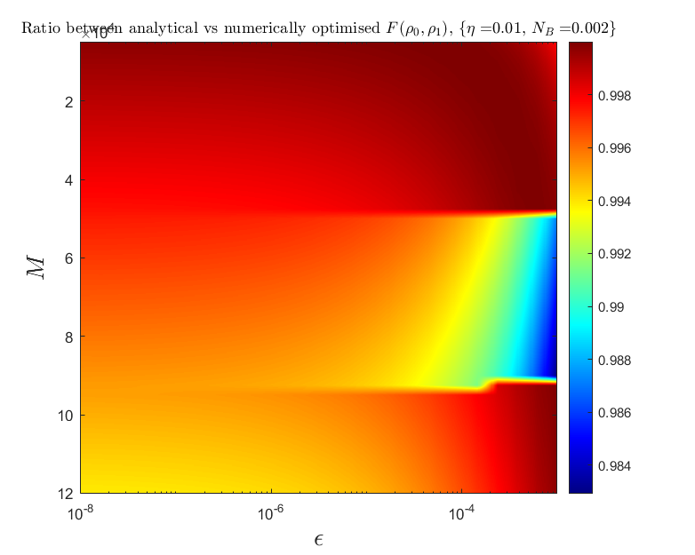
(a) $N_{B}=0.002$

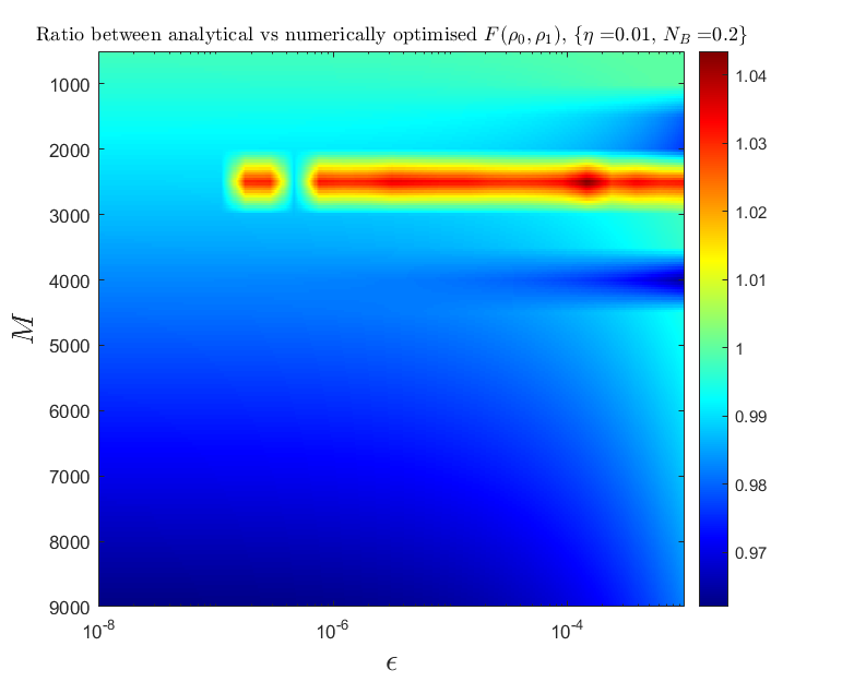
(b) $N_{B}=0.2$

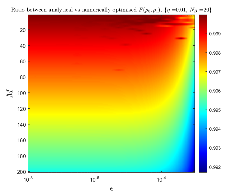
(c) $N_{B}=20$

Figure 4: Ratio of the analytical lower bound of Eq. (91) to the numerically minimized fidelity under $\epsilon-$ covertness.

VII.3 Performance of TMSV and GCS probes under $\epsilon-$covertness

When either TMSV or GCS states are used as probes by Alice, the states intercepted by Willie will be thermal states. To ensure that we use a brightness $N_{S}$ for these states that satisfies $P_{\mathfrak{e}}^{W}\geq 1/2-\epsilon$, we use the Fuchs-van de Graaf inequality and require that

$$\frac{1}{2}-\frac{\sqrt{1-F(\sigma_{0},\sigma_{1})^{2M}}}{2}\geq\frac{1}{2}-\epsilon$$

$$1-\sqrt{1-\left(\frac{1}{\sqrt{(N_{B}+1)(N+1)}-\sqrt{N_{B}N}}\right)^{2M}}\geq 1-2\epsilon$$ (117)

where $N=(1-\eta)N_{S}+\eta N_{B}$ is the brightness of $\sigma_{1}$. Solving for $N$ numerically, we obtain a maximum $N_{S}$ such that TMSV or GCS probes of that brightness are guaranteed to be $\epsilon$-covert. Using the quantum Chernoff bound, we calculate the performance of TMSV and GCS states shown in Fig. 4 of the main paper.

References

Tan et al. [2008]S.-H. Tan, B. I. Erkmen,
V. Giovannetti, S. Guha, S. Lloyd, L. Maccone, S. Pirandola, and J. H. Shapiro, Quantum illumination with Gaussian states, Phys. Rev. Lett. 101, 253601 (2008).
Mandel and Wolf [1995]L. Mandel and E. Wolf, Optical Coherence and Quantum
Optics (Cambridge University Press, Cambridge, 1995).
Pirandola et al. [2018]S. Pirandola, B. R. Bardhan, T. Gehring,
C. Weedbrook, and S. Lloyd, Advances in photonic quantum sensing, Nature Photonics 12, 724 (2018).
Torrome and Barzanjeh [2023]R. G. Torrome and S. Barzanjeh, Advances in quantum
radar and quantum lidar, arXiv preprint arXiv:2310.07198 (2023).
Bash et al. [2015]B. A. Bash, A. H. Gheorghe,
M. Patel, J. L. Habif, D. Goeckel, D. Towsley, and S. Guha, Quantum-secure covert communication on bosonic channels, Nature Communications 6, 1 (2015).
Gagatsos et al. [2019]C. N. Gagatsos, B. A. Bash,
A. Datta, Z. Zhang, and S. Guha, Covert sensing using floodlight illumination, Phys. Rev. A 99, 062321 (2019).
Hao et al. [2022]S. Hao, H. Shi, C. N. Gagatsos, M. Mishra, B. Bash, I. Djordjevic, S. Guha,
Q. Zhuang, and Z. Zhang, Demonstration of entanglement-enhanced covert sensing, Phys. Rev. Lett. 129, 010501 (2022).
Shapiro et al. [2019]J. H. Shapiro, D. M. Boroson, P. B. Dixon,
M. E. Grein, and S. A. Hamilton, Quantum low probability of
intercept, J. Opt. Soc. Am. B 36, B41 (2019).
Note [1]If the radar configuration is bistatic, we assume that the
idler modes can be transported losslessly to the receiver’s
location.
Note [2] represents the residual reflectivity in the entire
trip from transmitter to receiver and thus includes diffraction losses as
well as the reflectivity of the target object itself.
Nair et al. [2022]R. Nair, G. Y. Tham, and M. Gu, Optimal gain sensing of quantum-limited
phase-insensitive amplifiers, Phys. Rev. Lett. 128, 180506 (2022).
Shi and Zhuang [2023]H. Shi and Q. Zhuang, Ultimate precision limit of noise
sensing and dark matter search, npj Quantum Information 9, 27 (2023).
Nair and Gu [2023]R. Nair and M. Gu, Quantum sensing of phase-covariant optical
channels (2023), arXiv:2306.15256 [quant-ph] .
Nair and Gu [2020]R. Nair and M. Gu, Fundamental limits of quantum
illumination, Optica 7, 771 (2020).
Volkoff [2023]T. J. Volkoff, Not even 6 dB: Gaussian
quantum illumination in thermal background (2023), arXiv:2309.10071 [quant-ph]
.
Serafini [2017]A. Serafini, Quantum Continuous
Variables: A Primer of Theoretical Methods (CRC
Press, 2017).
Helstrom [1976]C. W. Helstrom, Quantum Detection and
Estimation Theory (Academic Press, New York, 1976).
Audenaert et al. [2007]K. M. R. Audenaert, J. Calsamiglia, R. Muñoz
Tapia, E. Bagan,
L. Masanes, A. Acín, and F. Verstraete, Discriminating states: The quantum Chernoff bound, Phys. Rev. Lett. 98, 160501 (2007).
Caruso et al. [2006]F. Caruso, V. Giovannetti, and A. S. Holevo, One-mode bosonic
Gaussian channels: a full weak-degradability classification, New Journal of Physics 8, 310 (2006).
Banchi et al. [2020]L. Banchi, Q. Zhuang, and S. Pirandola, Quantum-enhanced barcode decoding and
pattern recognition, Phys. Rev. Applied 14, 064026 (2020).
Zhuang and Pirandola [2020]Q. Zhuang and S. Pirandola, Entanglement-enhanced
testing of multiple quantum hypotheses, Communications Physics 3, 103 (2020).
Pereira et al. [2021]J. L. Pereira, L. Banchi,
Q. Zhuang, and S. Pirandola, Idler-free channel position finding, Phys. Rev. A 103, 042614 (2021).
Banchi et al. [2015]L. Banchi, S. L. Braunstein, and S. Pirandola, Quantum fidelity for
arbitrary Gaussian states, Phys. Rev. Lett. 115, 260501 (2015).
Sharma et al. [2018]K. Sharma, M. M. Wilde,
S. Adhikari, and M. Takeoka, Bounding the energy-constrained quantum and
private capacities of phase-insensitive bosonic Gaussian channels, New Journal of Physics 20, 063025 (2018).
Nair [2018]R. Nair, Quantum-limited loss
sensing: Multiparameter estimation and Bures distance between loss
channels, Phys. Rev. Lett. 121, 230801 (2018).
Nielsen and Chuang [2000]M. A. Nielsen and I. L. Chuang, Quantum Computation and
Quantum Information (Cambridge University Press,
Cambridge, UK, 2000).
Nair [2011]R. Nair, Discriminating
quantum-optical beam-splitter channels with number-diagonal signal states:
Applications to quantum reading and target detection, Phys. Rev. A 84, 032312 (2011).
Haus [2000]H. A. Haus, Electromagnetic noise and
quantum optical measurements (Springer Science &
Business Media, New York, 2000).