ITERATIVE SHALLOW FUSION OF BACKWARD LANGUAGE MODEL
FOR END-TO-END SPEECH RECOGNITION

Abstract

We propose a new shallow fusion (SF) method to exploit an external backward language model (BLM) for end-to-end automatic speech recognition (ASR). The BLM has complementary characteristics with a forward language model (FLM), and the effectiveness of their combination has been confirmed by rescoring ASR hypotheses as post-processing. In the proposed SF, we iteratively apply the BLM to partial ASR hypotheses in the backward direction (i.e., from the possible next token to the start symbol) during decoding, substituting the newly calculated BLM scores for the scores calculated at the last iteration. To enhance the effectiveness of this iterative SF (ISF), we train a partial sentence-aware BLM (PBLM) using reversed text data including partial sentences, considering the framework of ISF. In experiments using an attention-based encoder-decoder ASR system, we confirmed that ISF using the PBLM shows comparable performance with SF using the FLM. By performing ISF, early pruning of prospective hypotheses can be prevented during decoding, and we can obtain a performance improvement compared to applying the PBLM as post-processing. Finally, we confirmed that, by combining SF and ISF, further performance improvement can be obtained thanks to the complementarity of the FLM and PBLM.

Index Terms—  End-to-end speech recognition, shallow fusion, forward language model, iterative shallow fusion, partial sentence-aware backward language model

1 Introduction

Thanks to the significant progress in neural network (NN) modeling, the performance of automatic speech recognition (ASR) has rapidly improved. It was reported in 2017 that a hybrid ASR system, which exploits neural acoustic modeling and neural language model (LM) rescoring (and also system combination), had surpassed human performance on the conversational speech recognition task [1, 2, 3]. The performance has been further improved by leveraging a fully neural end-to-end (E2E) architecture [4, 5].

The E2E ASR system can integrate an external LM trained using a large text corpus to improve the system performance [4, 5]. Various methods for integrating the external ($n$-gram or neural) LM have been proposed [6, 7, 8, 9, 10, 11, 12, 13, 14]. Shallow fusion (SF) [6, 7, 8, 9, 10, 11] is the most popular method that performs log-linear interpolation between scores obtained from the main ASR model and the external LM during decoding. SF is simple, but it shows comparable performance with the learning-based deep [6], cold [12], and component [13] fusion methods, which jointly fine-tune the main ASR model and the pre-trained external neural LM for their tighter integration [11, 13, 14]. The more recently proposed density ratio approach [14] and internal language model estimation [15, 16] intend to reduce the influence of the internal LM implicitly included in the main ASR model to enhance the effect of LM integration. These methods inherit SF’s simplicity and practicality (since they can be performed during decoding without requiring any model training) and outperform SF [5, 14, 15, 16]. We focus on simple SF in this study since it shows good enough performance [11].

Since ASR hypotheses are extended successively from the start of an input utterance during decoding (beam search), a forward LM (FLM) is a natural choice for SF [4, 6, 7, 8, 9, 10, 11]. In contrast, in post-processing, such as $N$-best rescoring and lattice rescoring, a backward LM (BLM) can also be used along with the FLM [1, 2, 17, 18, 19, 20]. The BLM has complementary characteristics with the FLM, and their combination can greatly improve the ASR performance. Besides, the post-processing is performed for completed (not partial) hypotheses after decoding, and the BLM can be easily applied to the hypotheses from their end-of-sequence ($\mathtt{<\!\!eos\!\!>}$) symbols. In other words, it is difficult to apply the BLM for partial hypotheses during decoding, since they do not have the $\mathtt{<\!\!eos\!\!>}$ symbols, and this can limit the effect of the BLM.

In this study, we propose a new SF method to exploit an external BLM. To the best of our knowledge, this is the first study to use the BLM in SF. We expect that, by applying the BLM along with an FLM during decoding (not as post-processing), more accurate LM scores can be given to partial ASR hypotheses, and thus we can prevent incorrect early beam pruning of the prospective hypotheses. Consequently, we can obtain a more accurate one-best hypothesis as the ASR result. In contrast to the conventional SF using the FLM, which can be performed cumulatively, SF using the BLM needs to be performed iteratively. When a possible next token is connected to a partial ASR hypothesis during decoding, we need to recalculate the BLM score for the entire hypothesis in the backward direction (i.e., from the possible next token to the start symbol) and substitute it for the score calculated at the last iteration. Moreover, to enhance the effectiveness of the proposed iterative SF (ISF), we train a partial sentence-aware BLM using reversed text data that includes partial sentences considering the framework of ISF. We conduct experiments on the TED talk corpus [21] using an attention-based encoder-decoder (AED) ASR system [22, 23, 24] as the E2E ASR system and long short-term memory (LSTM)-based recurrent NN LMs (LSTMLMs) [25, 26] as the external LMs. We show the effectiveness of the proposed ISF and the effectiveness of its combination with the conventional SF.

2 Iterative shallow fusion

We describe the framework of the proposed ISF, the computational cost reduction of ISF-based decoding, and a partial sentence-aware BLM suitable for ISF.

2.1 Framework of ISF

Figure 1 shows the framework of the proposed ISF using a BLM. Let ${\mathbf{X}}$ be a hidden state vector sequence for an input utterance obtained from the encoder of an AED ASR model. Given ${\mathbf{X}}$, we perform decoding with SF using an FLM and ISF with a BLM on the decoder of the AED ASR model. Let $\left\{\mathtt{<\!\!sos\!\!>},w_{1:t-1}\right\}$ be a partial hypothesis (token sequence) of length $t-1$ and $w_{t}$ be a possible next token connected to $\left\{\mathtt{<\!\!sos\!\!>},w_{1:t-1}\right\}$, where $\mathtt{<\!\!sos\!\!>}$ is the start-of-sequence symbol that is excluded from the hypothesis length count. We calculate the score (log probability) of the extended partial hypothesis $\left\{\mathtt{<\!\!sos\!\!>},w_{1:t}\right\}$ given ${\mathbf{X}}$ as,

$$\log{P(\left\{\mathtt{<\!\!sos\!\!>},w_{1:t}\right\}|{\mathbf{X}})}$$

$$=\log{P(\left\{\mathtt{<\!\!sos\!\!>},w_{1:t-1}\right\}|{\mathbf{X}})}$$ (1a)

$$\hskip 10.243pt+\log{P_{\mathtt{dec}}(w_{t}|{\mathbf{X}},\left\{\mathtt{<\!\!sos\!\!>},w_{1:t-1}\right\})}$$ (1b)

$$\hskip 10.243pt+\alpha\log{P_{\mathtt{flm}}(w_{t}|\left\{\mathtt{<\!\!sos\!\!>},w_{1:t-1}\right\})}$$ (1c)

$$\hskip 10.243pt+\beta\left[\hskip 0.7113pt\log{P_{\mathtt{blm}}(\left\{\mathtt{<\!\!eos\!\!>},w_{t:1},\mathtt{<\!\!sos\!\!>}\right\})}\right.$$

$$\hskip 17.64069pt\left.-\hskip 2.84526pt\log{P_{\mathtt{blm}}(\left\{\mathtt{<\!\!eos\!\!>},w_{t-1:1},\mathtt{<\!\!sos\!\!>}\right\})}\hskip 0.7113pt\right]$$ (1d)

$$\hskip 10.243pt+\,\gamma,$$ (1e)

where the first term on the right side of this equation (Term (1a)) is the score of $\left\{\mathtt{<\!\!sos\!\!>},w_{1:t-1}\right\}$ given ${\mathbf{X}}$, Term (1b) is the score of $w_{t}$ given ${\mathbf{X}}$ and $\left\{\mathtt{<\!\!sos\!\!>},w_{1:t-1}\right\}$ obtained from the decoder of the E2E ASR model, Term (1c) is the score of $w_{t}$ given $\{\mathtt{<\!\!sos\!\!>},w_{1:t-1}\}$ obtained by the conventional SF using the FLM scaled by weight $\alpha$ ($\alpha\geq 0$), $\mathtt{<\!\!sos\!\!>}$ is used to start FLM calculation in the forward direction, Term (1d) is the score obtained by the proposed ISF using the BLM scaled by weight $\beta$ ($\beta\geq 0$), and the last Term (1e) is the reward $\gamma$ ($\gamma\geq 0$) given proportional to the sequence length [5, 7, 14]. The two BLM scores in Term (1d) can be rewritten as,

$$\log{P_{\mathtt{blm}}(\left\{\mathtt{<\!\!eos\!\!>},w_{t:1},\mathtt{<\!\!sos\!\!>}\right\})}$$ (2)

$$= \log{P_{\mathtt{blm}}(\mathtt{<\!\!eos\!\!>})}$$

$$+\log{{\textstyle\prod_{\tau=t}^{1}}P_{\mathtt{blm}}(w_{\tau}|\left\{\mathtt{<\!\!eos\!\!>},w_{t:\tau+1}\right\})}$$

$$+\log{P_{\mathtt{blm}}(\mathtt{<\!\!sos\!\!>}|\left\{\mathtt{<\!\!eos\!\!>},w_{t:1}\right\})},$$

$$\log{P_{\mathtt{blm}}(\left\{\mathtt{<\!\!eos\!\!>},w_{t-1:1},\mathtt{<\!\!sos\!\!>}\right\})}$$ (3)

$$= \log{P_{\mathtt{blm}}(\mathtt{<\!\!eos\!\!>})}$$

$$+\log{{\textstyle\prod_{\tau=t-1}^{1}}P_{\mathtt{blm}}(w_{\tau}|\left\{\mathtt{<\!\!eos\!\!>},w_{t-1:\tau+1}\right\})}$$

$$+\log{P_{\mathtt{blm}}(\mathtt{<\!\!sos\!\!>}|\left\{\mathtt{<\!\!eos\!\!>},w_{t-1:1}\right\})},$$

where $\mathtt{<\!\!eos\!\!>}$ is the temporarily connected end-of-sequence symbol used to start BLM calculation in the backward direction.

As can be seen in Fig. 1 and Term (1c), we can perform the conventional SF using the FLM cumulatively. At every timestep $t$, we calculate the FLM score of $w_{t}$ conditioned on $\{\mathtt{<\!\!sos\!\!>},w_{1:t-1}\}$, and the calculated score of $w_{t}$ does not change during decoding for the input utterance. In contrast, we cannot perform SF using the BLM cumulatively. The BLM score of $w_{\tau}$ changes during decoding when we extend the hypothesis with a new token, i.e., the condition $\{\mathtt{<\!\!eos\!\!>},w_{t:\tau+1}\}$ changes at every timestep $t$, as shown in Eq. (2).

Therefore, as shown in Fig. 1 and Term (1d), we need to perform SF using the BLM iteratively. In the proposed ISF, at every timestep $t$, we calculate the BLM score for the entire partial hypothesis $\{\mathtt{<\!\!eos\!\!>},w_{t:1},\mathtt{<\!\!sos\!\!>}\}$, as shown in Eq. (2). Furthermore, since the BLM score at the last timestep (iteration) $t-1$ shown in Eq. (3) is included in Term (1a), we need to subtract the score from the term, as shown in Term (1d).

As shown in Fig. 1, we also calculate the BLM score for the hypothesis that reaches the real (not temporal) $\mathtt{<\!\!eos\!\!>}$, i.e., for the completed (not a partial) hypothesis, as a kind of post-processing. However, this post-processing is different from conventional post-processing [1, 2, 17, 18, 19, 20]. The conventional post-processing is performed for a limited number of hypotheses (e.g., $N$-best list) after decoding. In contrast, this post-processing is performed for all the hypotheses that reach $\mathtt{<\!\!eos\!\!>}$ during decoding. Consequently, this post-processing is richer than the conventional post-processing.

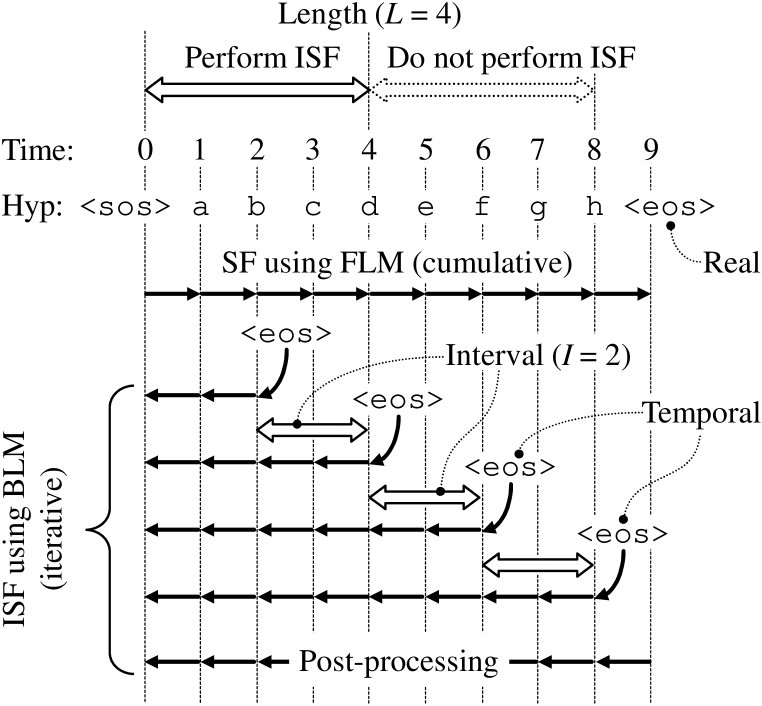
Fig. 1: Framework of the proposed ISF using a BLM. $\mathtt{<\!\!sos\!\!>}$ and $\mathtt{<\!\!eos\!\!>}$ are the start and (temporal or real) end symbols of an ASR hypothesis (token sequence), respectively. An alphabet corresponds to a token (e.g., a word, a subword, or a character).

2.2 Reducing computational cost of ISF-based decoding

We employ the standard label (token) synchronous beam search as the decoding algorithm [22, 24]. As described above, it is obvious that the computational cost of ISF is high, and we introduce a two-step pruning scheme into the decoding algorithm. Let $B$ be the beam size and $V$ be the vocabulary size (number of unique tokens, $V\hskip 0.31297pt{\gg}\hskip 0.31297ptB$). At every timestep $t$, each of the $B$ partial hypotheses can be extended with $V$ tokens, i.e., there are $B$ $\times$ $V$ possible partial hypotheses. Since it is difficult to perform ISF for all of these $B$ $\times$ $V$ hypotheses, we perform the first pruning for these hypotheses based on the scores obtained from the E2E ASR model and SF using the FLM to obtain the most probable $B$ $\times$ $B$ hypotheses. We then perform the second pruning for these $B$ $\times$ $B$ hypotheses based on the scores obtained from ISF using the BLM to obtain the most probable $B$ hypotheses, which are sent for processing at the next timestep. Note that, with this label synchronous beam search, the lengths (number of tokens) of partial hypotheses are the same during decoding, and we can introduce batch calculation to efficiently perform ISF for the $B$ $\times$ $B$ hypotheses.

Another idea to reduce the computational cost is to perform ISF not at every timestep but at every $I$ ($I\geq 1$) timestep, as shown in Fig. 1. In this case, the BLM score shown in Eq. (3) is replaced by the following score,

$$\log{P_{\mathtt{blm}}(\left\{\mathtt{<\!\!eos\!\!>},w_{t-I:1},\mathtt{<\!\!sos\!\!>}\right\})}$$ (4)

$$= \log{P_{\mathtt{blm}}(\mathtt{<\!\!eos\!\!>})}$$

$$+\log{{\textstyle\prod_{\tau=t-I}^{1}}P_{\mathtt{blm}}(w_{\tau}|\left\{\mathtt{<\!\!eos\!\!>},w_{t-I:\tau+1}\right\})}$$

$$+\log{P_{\mathtt{blm}}(\mathtt{<\!\!sos\!\!>}|\left\{\mathtt{<\!\!eos\!\!>},w_{t-I:1}\right\})},$$

and the computational cost of ISF is reduced by a factor of $I$.

As described in Section 1, we expect that, by performing ISF, we can prevent incorrect early pruning of prospective hypotheses. In other words, to keep the prospective hypotheses alive during decoding, it may be more important to perform ISF at the earlier stage of decoding rather than performing it at the later stage of decoding. To confirm this prediction and to reduce the computational cost, as shown on the top of Fig. 1, we perform ISF only during a partial hypothesis is not longer than $L$ tokens (excluding $\mathtt{<\!\!sos\!\!>}$ from the count) and do not perform ISF after the hypothesis gets longer than $L$ tokens until the last post-processing step (i.e., we perform post-processing even when we limit the length $L$).

In preliminary experiments, we confirmed that, even though applying the above three cost reduction methods, the computational cost of ISF remains relatively high. Further reduction of the computational cost of ISF is our future work. In this study, we investigate in Section 4 the effect of ISF on reducing word error rates (WERs) by changing the interval $I$ and limiting the length $L$.

Fig. 2: Reversed text data including partial sentences (token sequences) considering the framework of ISF used to train a PBLM.

2.3 Partial sentence-aware BLM (PBLM) suitable for ISF

As described in Section 2.1 and shown in Fig. 1, ISF can be started from a token at any timestep in an ASR hypothesis. This indicates that a normal BLM, which is trained using reversed text data, is not necessarily suitable for ISF, since it models token sequences starting from the end of complete sentences, whereas we need to apply it to partial hypotheses.

To enhance the effectiveness of ISF, we propose using a PBLM that can be more suitable for ISF than the normal BLM. As shown in Fig. 2, we prepare text data for training the PBLM considering the framework of ISF. We first reverse a sentence (used to train an FLM) and obtain the reversed sentence (used to train the normal BLM). Then, we shorten the reversed sentence step-by-step by removing the last token from the sentence at each step (i.e., interval $I$ is set at 1) and obtain reversed partial sentences used to train the PBLM. The text data used to train the PBLM is greatly augmented compared with those used to train the FLM or the normal BLM. We experimentally investigate which of the normal BLM or the PBLM is more suitable for ISF in Section 4.

3 Relation to prior work

As described in Section 1, the proposed ISF is an extension of SF [6, 7, 8, 9, 10, 11] and, to the best of our knowledge, this is the first study to use a BLM in SF. By performing ISF along with SF using an FLM, we intend to obtain performance improvement based on the complementarity of the FLM and the BLM, whose effectiveness has been confirmed in many studies for post-processing ($N$-best and lattice rescoring) of ASR hypotheses [1, 2, 17, 18, 19, 20]. In [27], the authors use a bidirectional LM for connectionist temporal classification (CTC) [28] based bidirectional greedy decoding. In contrast, in this study, we use both the FLM and BLM individually for unidirectional decoding.

This study is inspired by [29], in which the authors developed a real-time closed captioning system for broadcast news based on a two-pass ASR decoder. The system progressively outputs partial ASR results during decoding (i.e., streaming). There are many differences between [29] and our study, such as their aims (streaming ASR allowing a slight performance degradation vs. ASR performance improvement) and their model architectures (traditional GMM/HMM-based vs. recent NN-based). However, these two studies share the concept of performing rescoring during decoding with a fixed interval.

Table 1: Details of the TED-LIUM2 train/dev/test datasets.

	Train	Dev	Test
Hours	210.6	1.6	2.6
# utterances (sentences)	92791	507	1155
# words	2210368	17783	27500
# tokens (subwords)	4208823	34160	51179
Average length (# tokens)	45.4	67.4	44.3

Table 2: Text datasets to train an external FLM, BLM, and PBLM.

	FLM/BLM	PBLM
# sentences	13M	495M
# tokens (subwords)	482M	14G
Average length (# tokens)	37.1	27.6

4 Experiments

We conducted experiments based on an ESPnet ASR recipe using the TED-LIUM2 corpus [24, 21]. We used an AED ASR model [22, 23] consisting of a Conformer-based encoder [30] and a Transformer-based decoder [31] (and also a CTC [28] module) as the E2E ASR model and LSTMLMs [25, 26] as the external LMs. Details of the model structures and the training/decoding settings can be found in the recipe [24]. We used PyTorch [32] for all the NN modeling in this study.

4.1 Experimental settings

Table 2 shows the details of the TED-LIUM2 training, development, and test datasets [21]. We trained a SentencePiece model [33] using the word-based text training data and tokenized the word-based text training, development, and test datasets to obtain their token (subword)-based versions. We set the vocabulary size (number of unique tokens) $V$ at 500. Using the training data, we trained the AED ASR model (# encoder / decoder layers $=$ $17$ / $4$, # encoder / decoder units $=$ $1024$ / $1024$, # attention dimensions / heads $=$ $512$ / $4$) [22, 23]. We did not perform speed perturbation [34] and SpecAugment [35] in this study.

Table 2 shows the text datasets to train an external FLM, BLM, and PBLM. We prepared the PBLM training data with the procedure described in Section 2.3, which resulted in a significant data augmentation. All the LMs are the LSTMLMs [25, 26] sharing the same structure, i.e., four LSTM layers (each of them has 2048 units) and a softmax output layer of the vocabulary size ($V$ $=$ $500$). We trained these LMs using each of the training datasets with the stochastic gradient descent (SGD) optimizer for two epochs.

Using the AED ASR model and the three external LMs, we performed ASR based on the decoding algorithm described in Section 2.2. We set the beam size $B$ at ten and optimized the three weighting factors ($\alpha$, $\beta$, $\gamma$) shown in Eq. (1) using the development data. We set them at (0.5, 0.0, 2.0) when we performed SF using the FLM, at (0.0, 0.5, 2.0) when we performed ISF using the BLM or PBLM, and at (0.5, 0.5, 5.0) when we performed both SF and ISF. We performed decoding on a token basis but evaluated the ASR performance with WERs.

4.2 LM evaluation based on perplexities

Before showing the ASR results, we show the LM evaluation results with token-based perplexities. To calculate perplexities, we prepared two types of text datasets. One is the standard dataset that contains only complete sentences, and the other is that also includes partial sentences, as described in Section 2.3 and shown in Fig. 2.

Table 3 shows the token-based development and test data perplexities obtained with the FLM, BLM, and PBLM. Considering the vocabulary size ($V\!=\!500$), these perplexity values are reasonable. We can confirm that the BLM shows slightly better performance than the PBLM for the “only complete” sentences case, in contrast, the PBLM shows slightly better performance than the BLM for the “including partial” sentences case. These results suggest that the PBLM would be more suitable for ISF than the BLM.

Table 3: Token-based dev/test data (only complete / including partial sentences) perplexities obtained with the FLM, BLM, and PBLM.

	Only complete		Including partial
Model	Dev	Test	Dev	Test
FLM	10.2	11.8	—	—
BLM	10.1	11.8	15.1	17.1
PBLM	10.6	12.2	14.7	16.0

4.3 Comparison of SF methods and effect of interval

Table 4 shows the comparison results of the SF methods and the effect of interval $I$ for applying ISF (Section 2.2 and Fig. 1). We set interval $I$ at 1, 2, 5, 10, and $\infty$. Here, $I\!=\!\infty$ means that we do not perform ISF for partial hypotheses but perform it only for completed hypotheses as a kind of post-processing (Section 2.1 and Fig. 1). First, we can confirm that SF using the FLM (hereafter referred to as SF-FLM) steadily reduces the WERs from the baseline that does not perform SF (W/o SF) as reported in the previous studies [4, 5, 6, 7, 8, 9, 10, 11, 12, 13, 14].

Next, by comparing the results of ISF-PBLM (methods 7 to 11) with those of ISF-BLM (methods 2 to 6), ISF-PBLM performs better on the development data and comparably or slightly better on the test data. This improvement is supported by the better modeling capability of the PBLM for partial hypotheses, as we confirmed in Section 4.2. We can also confirm that ISF-PBLM performs comparably with SF-FLM. As regards interval $I$, smaller values (e.g., 1 or 2) are better than larger values (except for the results of ISF-BLM for the development data). From these results, we can confirm that it is important to perform ISF not only for completed hypotheses as post-processing but also for partial hypotheses during decoding.

Finally, we can confirm that, by combining SF-FLM and ISF-PBLM (methods 12 to 16, SF-FLM+ISF-PBLM), we can obtain further performance improvement compared with when performing SF or ISF individually. This improvement is achieved thanks to the complementarity of the FLM and PBLM [1, 2, 17, 18, 19, 20]. Also in this case, we can confirm the importance of performing ISF for partial hypotheses during decoding. SF-FLM+ISF-PBLM with $I\!=\!2$ achieves about 8% relative WER reductions from SF-FLM, and these reductions are statistically significant at the 1% level.

4.4 Effect of limiting partial hypothesis length to apply ISF

As described in Section 2.2 and shown in Fig. 1, we investigated the effect of limiting the partial hypothesis length $L$ (i.e., the first $L$ tokens) to apply ISF-PBLM. We employed method 12, shown in Table 4, i.e., SF-FLM+ISF-PBLM with interval $I\!=\!1$. By setting $I$ at 1, the number of times we apply ISF becomes equal to the length of the partial hypothesis. We also employed SF-FLM+ISF-PBLM with $I\!=\!1$ but without performing post-processing as another version of method 12, i.e., method 12^′, to exclude (and also to confirm) the effect of post-processing. We conducted experiments on the development data by setting $L$ at 10, 20, 30, 50, and $\infty$, since the average length (number of tokens) of the utterances in the development data is 67.4, as shown in Table 2. Here, $L\!=\!\infty$ means that we do not limit the length, i.e., the default setting.

Figure 3 shows WERs as a function of the partial hypothesis length $L$ to apply ISF-PBLM. As can be seen in the result of method 12^′, even with $L\!=\!10$, we can obtain a steady WER reduction from the SF-FLM baseline (14.6%). At the same time, we can confirm that, contrary to our prediction described in Section 2.2, performing ISF at the later stage of decoding is also important as performing it at the earlier stage, since the WER is gradually reduced by lengthening $L$. However, from the result of method 12, we can confirm that, with the help of post-processing, we can limit $L$ by 30 (tokens), i.e., about half the length of the complete sentence on average. This result supports our prediction to some extent.

Table 4: Comparison of the SF methods and the effect of the interval for applying ISF on the development and test datasets.

No.	Method	Interval ($I$)	Dev	Test
0.	W/o SF	—	15.4	11.2
1.	SF-FLM	—	14.6	9.9
2.	ISF-BLM	1	15.1	10.1
3.		2	14.9	10.2
4.		5	15.0	10.3
5.		10	15.1	10.3
6.		$\infty$  (post-proc.)	14.8	10.5
7.	ISF-PBLM	1	14.2	10.1
8.		2	14.2	10.0
9.		5	14.4	10.2
10.		10	14.7	10.3
11.		$\infty$  (post-proc.)	14.8	10.5
12.	SF-FLM + ISF-PBLM	1	13.6	9.2
13.		2	13.5	9.1
14.		5	14.0	9.2
15.		10	13.8	9.3
16.		$\infty$  (post-proc.)	13.9	9.4

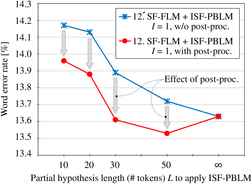
Fig. 3: Effect of limiting the partial hypothesis length $L$ (# tokens) to apply ISF-PBLM and that of post-processing on the dev data.

5 Conclusion and future work

We proposed a new shallow fusion method, i.e., iterative shallow fusion (ISF), using a backward LM for E2E ASR and showed its effectiveness experimentally. Future work will include further computational cost reduction of ISF (Section 2.2), evaluation using other ASR tasks, implementation on other E2E ASR models [36, 37, 16], and combination with other LM integration methods [14, 15, 16].

References

- [1] W. Xiong et al., “Achieving human parity in conversational speech recognition,” arXiv:1610.05256v2 [cs.CL].
- [2] ——, “Toward human parity in conversational speech recognition,” IEEE/ACM Transactions on Audio, Speech, and Language Processing, vol. 25, no. 12, pp. 2410–2423, Dec. 2017.
- [3] G. Saon et al., “English conversational telephone speech recognition by humans and machines,” in Proc. Interspeech, 2017, pp. 132–136.
- [4] Z. Tüske, G. Saon, K. Audhkhasi, and B. Kingsbury, “Single headed attention based sequence-to-sequence model for state-of-the-art results on Switchboard,” in Proc. Interspeech, 2020, pp. 551–555.
- [5] Z. Tüske, G. Saon, and B. Kingsbury, “On the limit of English conversational speech recognition,” in Proc. Interspeech, 2021, pp. 2062–2066.
- [6] C. Gulcehre et al., “On using monolingual corpora in neural machine translation,” arXiv:1503.03535v2 [cs.CL].
- [7] D. Bahdanau, J. Chorowski, D. Serdyuk, P. Brakel, and Y. Bengio, “End-to-end attention-based large vocabulary speech recognition,” in Proc. ICASSP, 2016, pp. 4945–4949.
- [8] J. Chorowski and N. Jaitly, “Towards better decoding and language model integration in sequence to sequence models,” in Proc. Interspeech, 2017, pp. 523–527.
- [9] T. Hori, S. Watanabe, Y. Zhang, and W. Chan, “Advances in joint CTC-attention based end-to-end speech recognition with a deep CNN encoder and RNN-LM,” in Proc. Interspeech, 2017, pp. 949–953.
- [10] A. Kannan, Y. Wu, P. Nguyen, T. N. Sainath, Z. Chen, and R. Prabhavalkar, “An analysis of incorporating an external language model into a sequence-to-sequence model,” in Proc. ICASSP, 2018, pp. 5824–5828.
- [11] S. Toshniwal, A. Kannan, C.-C. Chiu, Y. Wu, T. N. Sainath, and K. Livescu, “A comparison of techniques for language model integration in encoder-decoder speech recognition,” in Proc. SLT, 2018, pp. 369–375.
- [12] A. Sriram, H. Jun, S. Satheesh, and A. Coates, “Cold fusion: Training Seq2Seq models together with language models,” in Proc. Interspeech, 2018, pp. 387–391.
- [13] C. Shan et al., “Component fusion: Learning replaceable language model component for end-to-end speech recognition system,” in Proc. ICASSP, 2019, pp. 5631–5635.
- [14] E. McDermott, H. Sak, and E. Variani, “A density ratio approach to language model fusion in end-to-end automatic speech recognition,” in Proc. ASRU, 2019, pp. 434–441.
- [15] Z. Meng et al., “Internal language model estimation for domain-adaptive end-to-end speech recognition,” in Proc. SLT, 2021, pp. 243–250.
- [16] T. Moriya et al., “Hybrid RNN-T/Attention-based streaming ASR with triggered chunkwise attention and dual internal language model integration,” in Proc. ICASSP, 2022, pp. 8282–8286.
- [17] K. Irie, Z. Lei, L. Deng, R. Schlüter, and H. Ney, “Investigation on estimation of sentence probability by combining forward, backward and bi-directional LSTM-RNNs,” in Proc. Interspeech, 2018, pp. 392–395.
- [18] N. Kanda et al., “The Hitachi/JHU CHiME-5 system: Advances in speech recognition for everyday home environments using multiple microphone arrays,” in Proc. of The 5th Intl. Workshop on Speech Processing in Everyday Environments (CHiME 2018), 2018.
- [19] A. Arora et al., “The JHU multi-microphone multi-speaker ASR system for the CHiME-6 challenge,” in Proc. of The 6th Intl. Workshop on Speech Processing in Everyday Environments (CHiME 2020), 2020.
- [20] A. Ogawa, N. Tawara, M. Delcroix, and S. Araki, “Lattice rescoring based on large ensemble of complementary neural language models,” in Proc. ICASSP, 2022, pp. 6517–6521.
- [21] A. Rousseau, P. Deléglise, and Y. Estève, “Enhancing the TED-LIUM corpus with selected data for language modeling and more TED talks,” in Proc. LREC, 2014, pp. 3935–3939.
- [22] S. Watanabe, T. Hori, S. Kim, J. R. Hershey, and T. Hayashi, “Hybrid CTC/Attention architecture for end-to-end speech recognition,” IEEE/ACM Transactions on Audio, Speech, and Language Processing, vol. 11, no. 8, pp. 1240–1253, Dec. 2017.
- [23] P. Guo et al., “Recent developments on ESPnet toolkit boosted by Conformer,” in Proc. ICASSP, 2021, pp. 5874–5878.
- [24] S. Watanabe, “ESPnet: End-to-end speech processing toolkit,” https://github.com/espnet/espnet.
- [25] S. Hochreiter and J. Schmidhuber, “Long short-term memory,” Neural Computation, vol. 9, no. 8, pp. 1735–1780, Nov. 1997.
- [26] M. Sundermeyer, R. Schlüter, and H. Ney, “LSTM neural networks for language modeling,” in Proc. Interspeech, 2012.
- [27] N. Jung, G. Kim, and H.-G. Kim, “Back from the future: Bidirectional CTC decoding using future information in speech recognition,” arXiv:2110.03326v1 [cs.CL].
- [28] A. Graves, S. Fernández, F. Gomez, and J. Schmidhuber, “Connectionist temporal classification: Labelling unsegmented sequence data with recurrent neural networks,” in Proc. ICML, 2006, pp. 369–376.
- [29] T. Imai, A. Kobayashi, S. Sato, H. Tanaka, and A. Ando, “Progressive 2-pass decoder for real-time broadcast news captioning,” in Proc. ICASSP, 2000, pp. 1599–1562.
- [30] A. Gulati et al., “Conformer: Convolution-augmented Transformer for speech recognition,” in Proc. Interspeech, 2020, pp. 5036–5040.
- [31] A. Vaswani et al., “Attention is all you need,” in Proc. NIPS, 2017, pp. 5998–6008.
- [32] A. Paszke et al., “PyTorch: An imperative style, high-performance deep learning library,” in Proc. NeurIPS, 2019, pp. 8024–8035.
- [33] T. Kudo and J. Richardson, “SentencePiece: A simple and language independent subword tokenizer and detokenizer for neural text processing,” in Proc. EMNLP, 2018, pp. 66–71.
- [34] T. Ko, V. Peddinti, D. Povey, and S. Khudanpur, “Audio augmentation for speech recognition,” in Proc. Interspeech, 2015, pp. 3586–3589.
- [35] D. S. Park et al., “SpecAugment: A simple data augmentation method for automatic speech recognition,” in Proc. Interspeech, 2019, pp. 2613–2617.
- [36] A. Graves, “Sequence transduction with recurrent neural networks,” in Proc. ICML, 2012.
- [37] G. Saon, Z. Tüske, and K. Audhkhasi, “Alignment-length synchronous decoding for RNN transducer,” in Proc. ICASSP, 2020, pp. 7804–7808.