Deterministic and Stochastic Accelerated Gradient Method for Convex Semi-Infinite Optimization

Abstract

This paper explores numerical methods for solving a convex differentiable semi-infinite program. We introduce a primal-dual gradient method which performs three updates iteratively: a momentum gradient ascend step to update the constraint parameters, a momentum gradient ascend step to update the dual variables, and a gradient descend step to update the primal variables. Our approach also extends to scenarios where gradients and function values are accessible solely through stochastic oracles. This method extends the recent primal-dual methods, for example, Hamedani and Aybat (2021); Boob et al. (2022), for optimization with a finite number of constraints. We show the iteration complexity of the proposed method for finding an $\epsilon$-optimal solution under different convexity and concavity assumptions on the functions.

1 Introduction

We consider the following constrained optimization problem

$$f^{*} := \min_{{\mathbf{x}}\in{\mathcal{X}}}f({\mathbf{x}})\quad\text{s.t.}\quad g_{i}({\mathbf{x}},{\mathbf{y}}^{i})\leq 0,~{}\forall{\mathbf{y}}^{i}\in{\mathcal{Y}}^{i},~{}i=1,\dots,m.$$ (1)

Here, $f$ and $g_{i}$, $i=1,\dots,m$ are real-valued continuous functions, and ${\mathcal{X}}\subset\mathbb{R}^{p}$ and ${\mathcal{Y}}^{i}\subset\mathbb{R}^{q}$, $i=1,\dots,m$ are convex closed sets. Since ${\mathcal{Y}}^{i}$ is not a finite set, the number of constraints in (1) is infinite, so (1) is a semi-infinite program (SIP) (Reemtsen and Rückmann, 1998; Goberna and Lopez, 2002; López and Still, 2007; Goberna and López, 2013, and references therein). SIP has been studied systematically since the 1970s and has a number of applications including robotics (Marin, 1988; Hettich and Still, 1991; Vaz et al., 2004), statistics (Dall’Aglio, 2001), machine learning (Özögür-Akyüz and Weber, 2009; Özöğür-Akyüz and Weber, 2010; Sonnenburg et al., 2006), stochastic programming (Dentcheva and Ruszczyński, 2004), robust optimization (Mehrotra and Papp, 2014; Liu et al., 2015; Sun et al., 2017; Luo and Mehrotra, 2017), Markov decision process (de Farias and Van Roy, 2003; Lin et al., 2020; Pakiman et al., 2020), inventory control (Adelman, 2004; Adelman and Klabjan, 2012; Adelman and Barz, 2013), revenue management (Adelman, 2007), queuing (Farias and Van Roy, 2007; Zhang and Adelman, 2009; Adelman and Mersereau, 2013), and health care (Patrick et al., 2008; Restrepo, 2008, ch. 4).

In this paper, we study the first-order method for finding an $\epsilon$-optimal solution for (1), which is a solution $\bar{\mathbf{x}}\in\mathcal{X}$ satisfying

$$f(\bar{\mathbf{x}})-f^{*}\leq\epsilon\text{ and }g_{i}^{*}(\bar{\mathbf{x}})\leq\epsilon,~{}i=1,\dots,m,$$ (2)

where

$$g_{i}^{*}({\mathbf{x}}):=\max_{{\mathbf{y}}^{i}\in\mathcal{Y}^{i}}g_{i}({\mathbf{x}},{\mathbf{y}}^{i}),~{}i=1,\dots,m.$$ (3)

To do so, the following assumptions are made for problem (1).

Assumption 1 (Convexity and compactness)

The following statements hold.

1. ${\mathcal{X}}\subset\mathbb{R}^{p}$ and ${\mathcal{Y}}^{i}\subset\mathbb{R}^{q}$, $i=1,\dots,m$ are convex and closed.

2. There exists $D_{y}$ such that $\|{\mathbf{y}}^{i}-{\mathbf{y}}^{i\prime}\|\leq D_{y}$ for any ${\mathbf{y}}^{i},{\mathbf{y}}^{i\prime}\in{\mathcal{Y}}^{i}$ for $i=1,\dots,m$.

3. $f$ is $\mu_{f}$-strongly convex in ${\mathbf{x}}$ for $\mu_{f}\geq 0$.

4. $g_{i}$ is convex in ${\mathbf{x}}$ for $i=1,\dots,m$.

5. $g_{i}$ is $\mu_{y}$-strongly concave in ${\mathbf{y}}^{i}$ for $i=1,\dots,m$ and $\mu_{y}\geq 0$.

Note that $\mu_{f}$ and $\mu_{y}$ can be zero. As shown in this paper, the theoretical iteration complexity of the studied method depends on whether $\mu_{f}$ or $\mu_{y}$ or both are positive. We can also assume $g_{i}$ is $\mu_{x}$-strongly convex in ${\mathbf{x}}$ for $i=1,\dots,m$ with $\mu_{x}\geq 0$. However, whether $\mu_{x}$ is positive or not does not affect the order of iteration complexity. This is consistent with the findings when there are finitely many constraints (Hamedani and Aybat, 2021; Boob et al., 2022). Hence, we do not introduce $\mu_{x}$ for simplicity. Here, we assume ${\mathcal{Y}}^{i}$ has the same dimension for $i=1,\dots,m$ only to simplify the notation. In fact, all the results in this paper still hold when each ${\mathcal{Y}}^{i}$ has its own dimension.

Let ${\boldsymbol{\lambda}}=(\lambda_{1},\dots,\lambda_{m})^{\top}\in\mathbb{R}_{+}^{m}$ be the Lagrangian multipliers of the constraints in (1). We assume that there exist Lagrangian multipliers that satisfy the optimality conditions together with the optimal solution of (1).

Assumption 2 (Existence of optimal multipliers)

For any optimal solution ${\mathbf{x}}^{*}$ of (1), there exists ${\boldsymbol{\lambda}}^{*}\in\mathbb{R}_{+}^{m}$ such that

$${\mathbf{x}}^{*}\in\operatorname*{arg\,min}_{{\mathbf{x}}\in{\mathcal{X}}}\left[f({\mathbf{x}})+({\boldsymbol{\lambda}}^{*})^{\top}{\mathbf{g}}^{*}({\mathbf{x}})\right]\text{ and }\lambda_{i}^{*}g_{i}^{*}({\mathbf{x}}^{*})=0,\quad i=1,\dots,m,$$

where

$${\mathbf{g}}^{*}({\mathbf{x}})=(g_{1}^{*}({\mathbf{x}}),\dots,g_{m}^{*}({\mathbf{x}}))^{\top}.$$ (4)

In addition, we assume $f$ and $g_{i}$, $i=1,\dots,m$, are real-valued and continuously differentiable. Let $\nabla f$ be the gradient of $f$ and let $\nabla_{x}g_{i}$ and $\nabla_{y}g_{i}$ be the gradient of $g$ with respect to ${\mathbf{x}}$ and ${\mathbf{y}}^{i}$, respectively. Let $\|\cdot\|$ denote the Euclidean norm throughout the paper. The following assumptions are also made.

Assumption 3 (Smoothness and Lipschitz continuity)

There exist non-negative constants $L_{f}$, $L_{g}^{xx}$, $L_{g}^{yx}$, $L_{g}^{yy}$, $M_{g}^{x}$ and $M_{g}^{y}$ such that the following statements hold.

1. $\|\nabla f({\mathbf{x}})-\nabla f({\mathbf{x}}^{\prime})\|\leq L_{f}\|{\mathbf{x}}-{\mathbf{x}}^{\prime}\|$ for any ${\mathbf{x}},{\mathbf{x}}^{\prime}\in{\mathcal{X}}$.

2. $\|\nabla_{x}g_{i}({\mathbf{x}},{\mathbf{y}}^{i})-\nabla_{x}g_{i}({\mathbf{x}}^{\prime},{\mathbf{y}}^{i})\|\leq L_{g}^{xx}\|{\mathbf{x}}-{\mathbf{x}}^{\prime}\|$ for any ${\mathbf{x}},{\mathbf{x}}^{\prime}\in{\mathcal{X}}$ and any ${\mathbf{y}}^{i}\in{\mathcal{Y}}^{i}$.

3. $\|\nabla_{y}g_{i}({\mathbf{x}},{\mathbf{y}}^{i})-\nabla_{y}g_{i}({\mathbf{x}}^{\prime},{\mathbf{y}}^{i\prime})\|\leq L_{g}^{yx}\|{\mathbf{x}}-{\mathbf{x}}^{\prime}\|+L_{g}^{yy}\|{\mathbf{y}}^{i}-{\mathbf{y}}^{i\prime}\|$ for any ${\mathbf{x}},{\mathbf{x}}^{\prime}\in{\mathcal{X}}$ and any ${\mathbf{y}}^{i},{\mathbf{y}}^{i\prime}\in{\mathcal{Y}}^{i}$.

4. $|g_{i}({\mathbf{x}},{\mathbf{y}}^{i})-g_{i}({\mathbf{x}}^{\prime},{\mathbf{y}}^{i\prime})|\leq M_{g}^{x}\|{\mathbf{x}}-{\mathbf{x}}^{\prime}\|+M_{g}^{y}\|{\mathbf{y}}^{i}-{\mathbf{y}}^{i\prime}\|$ for any ${\mathbf{x}},{\mathbf{x}}^{\prime}\in{\mathcal{X}}$ and any ${\mathbf{y}}^{i},{\mathbf{y}}^{i\prime}\in{\mathcal{Y}}^{i}$.

We consider both the case where the gradients and function values above can be computed exactly and the case where they can only be approximated by stochastic oracles. In the latter case, we call (1) a stochastic semi-infinite program (SSIP), for which the following standard assumptions are made.

Assumption 4 (Stochastic oracles)

There exist a random vector $\xi$ and mappings $\nabla F({\mathbf{x}},\xi)\in\mathbb{R}^{p}$, $G_{i}({\mathbf{x}},{\mathbf{y}}^{i},\xi)\in\mathbb{R}$, $\nabla_{x}G_{i}({\mathbf{x}},{\mathbf{y}}^{i},\xi)\in\mathbb{R}^{p}$, and $\nabla_{y}G_{i}({\mathbf{x}},{\mathbf{y}}^{i},\xi)\in\mathbb{R}^{q}$ that provide stochastic oracles for $\nabla f({\mathbf{x}})$, $g_{i}({\mathbf{x}},{\mathbf{y}}^{i})$, $\nabla_{x}g_{i}({\mathbf{x}},{\mathbf{y}}^{i})$, and $\nabla_{y}g_{i}({\mathbf{x}},{\mathbf{y}}^{i})$, respectively. Moreover, the following conditions hold.

Unbiasedness:

$$\mathbb{E}[\nabla F({\mathbf{x}},\xi)] = \nabla f({\mathbf{x}}),$$ (5)

$$\mathbb{E}[G_{i}({\mathbf{x}},{\mathbf{y}}^{i},\xi)] = g_{i}({\mathbf{x}},{\mathbf{y}}^{i}),\quad\quad i=1,\cdots,m$$ (6)

$$\mathbb{E}[\nabla_{x}G_{i}({\mathbf{x}},{\mathbf{y}}^{i},\xi)] = \nabla_{x}g_{i}({\mathbf{x}},{\mathbf{y}}^{i}),\quad\quad i=1,\cdots,m$$ (7)

$$\mathbb{E}[\nabla_{y}G_{i}({\mathbf{x}},{\mathbf{y}}^{i},\xi)] = \nabla_{y}g_{i}({\mathbf{x}},{\mathbf{y}}^{i}),\quad\quad i=1,\cdots,m.$$ (8)

Bounded variance:

$$\mathbb{E}[\|\nabla F({\mathbf{x}},\xi)-\nabla f({\mathbf{x}})\|^{2}] \leq \sigma_{f^{\prime}}^{2},$$ (9)

$$\mathbb{E}[\|G_{i}({\mathbf{x}},{\mathbf{y}}^{i},\xi)-g_{i}({\mathbf{x}},{\mathbf{y}}^{i})\|^{2}] \leq \sigma_{g}^{2},\quad\quad i=1,\cdots,m$$ (10)

$$\mathbb{E}[\|\nabla_{x}G_{i}({\mathbf{x}},{\mathbf{y}}^{i},\xi)-\nabla_{x}g_{i}({\mathbf{x}},{\mathbf{y}}^{i})\|^{2}] \leq \sigma_{g^{\prime}}^{2},\quad\quad i=1,\cdots,m$$ (11)

$$\mathbb{E}[\|\nabla_{y}G_{i}({\mathbf{x}},{\mathbf{y}}^{i},\xi)-\nabla_{y}g_{i}({\mathbf{x}},{\mathbf{y}}^{i})\|^{2}] \leq \sigma_{g^{\prime}}^{2},\quad\quad i=1,\cdots,m,$$ (12)

where $\sigma_{f^{\prime}}$, $\sigma_{g}$ and $\sigma_{g^{\prime}}$ are non-negative constants.

Let ${\mathcal{Y}}:={\mathcal{Y}}^{1}\times{\mathcal{Y}}^{2}\times\cdots\times{\mathcal{Y}}^{m}\subset\mathbb{R}^{mq}$ and ${\mathbf{y}}=({\mathbf{y}}^{1\top},\dots,{\mathbf{y}}^{m\top})^{\top}\in{\mathcal{Y}}$. Consider the Lagrangian function of (1)

$$\phi({\mathbf{x}},{\boldsymbol{\lambda}},{\mathbf{y}})=f({\mathbf{x}})+{\boldsymbol{\lambda}}^{\top}{\mathbf{g}}({\mathbf{x}},{\mathbf{y}}).$$ (13)

Given an optimal solution ${\mathbf{x}}^{*}$ and the Lagrangian multipliers ${\boldsymbol{\lambda}}^{*}$ in Assumption 2, let ${\mathbf{y}}^{*}\in\operatorname*{arg\,max}_{{\mathbf{y}}\in{\mathcal{Y}}}{\mathbf{g}}({\mathbf{x}}^{*},{\mathbf{y}})$. It is known that $({\mathbf{x}}^{*},{\boldsymbol{\lambda}}^{*},{\mathbf{y}}^{*})$ is a saddle-point of (13) in the sense that

$$\phi({\mathbf{x}}^{*},{\boldsymbol{\lambda}},{\mathbf{y}})\leq\phi({\mathbf{x}}^{*},{\boldsymbol{\lambda}}^{*},{\mathbf{y}}^{*})\leq\phi({\mathbf{x}},{\boldsymbol{\lambda}}^{*},{\mathbf{y}}^{*})$$

for any $({\mathbf{x}},{\boldsymbol{\lambda}},{\mathbf{y}})\in{\mathcal{X}}\times\mathbb{R}_{+}^{m}\times{\mathcal{Y}}$. This motivates using a primal-dual gradient method for finding a saddle-point of $\phi({\mathbf{x}},{\boldsymbol{\lambda}},{\mathbf{y}})$. However, Assumptions 1 only ensures the convexity of $\phi$ on ${\mathbf{x}}$ but not the joint concavity of $\phi$ on $({\boldsymbol{\lambda}},{\mathbf{y}})$, so one cannot directly apply the existing primal-dual methods for convex-concave min-max problems (e.g., (Hamedani and Aybat, 2021; Boob et al., 2022)) and their convergence analysis.

That being said, (1) should not be intractable with the convexity and concavity ensured by Assumptions 1. In fact, thanks to the concavity of $g_{i}$ in ${\mathbf{y}}^{i}$, one can at least solve the lower problems, $\max_{{\mathbf{y}}^{i}\in{\mathcal{Y}}^{i}}g_{i}({\mathbf{x}},{\mathbf{y}}^{i})$, $i=1,\dots,m$ for a desired optimality gap using an inner loop. The approximate solutions to the lower problems can be used to construct some inexact gradient of $g_{i}^{*}$, which allows us to solve (1) by some constrained optimization algorithms with inexact gradients. However, this approach involves double loops which are not easy to implement and the demanded quality of the solutions to the lower problems usually increases as the outer loop proceeds, potentially leading to high total complexity.

To address these issues, we propose a first-order algorithm that only performs one gradient ascend step on $g_{i}$ to update ${\mathbf{y}}^{i}$ in each iteration, followed by primal-dual gradient steps to update ${\boldsymbol{\lambda}}$ and ${\mathbf{x}}$ using the function values and gradients on the historical iterates. This way, the algorithm involves only a single-loop, which is easy to implement, and does not need to solve the lower problems explicitly for any precision. Since $({\boldsymbol{\lambda}},{\mathbf{y}})$ are not updated jointly, our convergence analysis bypasses the non-concavity of $\phi$, so we can show the number of iterations the proposed method needs to find an $\epsilon$-optimal solution of (1). The obtained iteration complexity depends on $\mu_{f}$ and $\mu_{y}$ as well as the type of gradient oracles (deterministic or stochastic) and is summarized in Table 1.

Method	$\mu_{f}$	$\mu_{y}$	Gradients	Oracles for lower problems	Iters
This paper	$>0$	$>0$	Deter.	$g_{i}$, $\nabla_{x}g_{i}$, $\nabla_{y}g_{i}$	$O(\epsilon^{-0.5})$
This paper	$>0$	$=0$	Deter.		$O(\epsilon^{-1})$
This paper	$=0$	$>0$	Deter.		$O(\epsilon^{-1})$
This paper	$=0$	$=0$	Deter.		$O(\epsilon^{-1})$
This paper	$=0$	$=0$	Stoch.	$G_{i}$, $\nabla_{x}G_{i}$, $\nabla_{y}G_{i}$	$O(\epsilon^{-2})$
Wei et al. (2020b)	$=0$	NA	Deter.	$g_{i}$, $\nabla_{x}g_{i}$, $\approx\operatorname*{arg\,max}\limits_{{\mathbf{y}}^{i}\in{\mathcal{Y}}^{i}}g_{i}({\mathbf{x}},{\mathbf{y}}^{i})$	$O(\epsilon^{-2})$
Wei et al. (2020b)	$>0$	NA	Deter.		$O(\epsilon^{-1})$
Wei et al. (2020a)	$=0$	NA	Deter.	$g_{i}$, $\nabla_{x}g_{i}$ or $G_{i}$, $\nabla_{x}G_{i}$,	$O(\epsilon^{-2})$
Lin et al. (2020)			Or Stoch.	sample from a density on ${\mathcal{Y}}^{i}$	$O(\epsilon^{-2})$

Table 1: Comparison of the oracles assumed by different methods and their iteration complexity.

This paper is not the first effort on developing first-order methods for SIP. Wei et al. (Wei et al., 2020a) propose primal-dual gradient methods for SIP and SSIP, where the dual variables are probability densities on ${\mathcal{Y}}^{i}$’s. They require sampling from ${\mathcal{Y}}^{i}$’s using those densities whose computational cost is high when ${\mathcal{Y}}^{i}$’s have a high dimension. Wei et al. also propose in Wei et al. (2020b) a cooperative (switching) gradient method for SIP where, in each iteration, they assume a nearly optimal solution to $\max_{{\mathbf{y}}^{i}\in{\mathcal{Y}}^{i}}g_{i}({\mathbf{x}},{\mathbf{y}}^{i})$ can be found. On the contrary, our method only needs to compute the (stochastic) gradients of $g_{i}$ and $f$ per iteration, which in general has significantly lower computational cost than the oracles (sampling over a density or solving a maximization problem) needed in Wei et al. (2020a, b). Note that, because of the strong oracles they assume, $g_{i}$ does not need to be concave in ${\mathbf{y}}^{i}$ in Wei et al. (2020a, b).

Despite using weaker oracles, our method needs the same or fewer iterations than Wei et al. (2020a, b) for finding an $\epsilon$-optimal solution. As presented in Table 1, our method needs only $O(\epsilon^{-1})$ iterations for SIP when $\mu_{f}=0$ and $\mu_{y}>0$ while the methods in Wei et al. (2020a, b) need $O(\epsilon^{-2})$ iterations if applied to the same problems. When $\mu_{f}>0$ and $\mu_{y}=0$, our method needs $O(\epsilon^{-1})$ iterations while Wei et al. (2020b) needs to further assume $g_{i}$ is strongly convex in ${\mathbf{x}}$ to achieve the same complexity. Overall, this paper is the first work that establishes the iteration complexity of a single-loop method for convex SIP and SSIP under the scenarios listed in Table 1 using only (stochastic) gradient oracles.

2 Related Works

SIP has been systematically discussed in several monographs (Reemtsen and Rückmann, 1998; Reemtsen and Görner, 1998; Goberna and Lopez, 2002; López and Still, 2007; Hettich and Kortanek, 1993; Goberna and López, 2013) and has many applications as listed in the previous section. Most numerical algorithms for optimization with finitely many constraints can be somehow extended for SIP. The examples include the penalty method (Conn and Gould, 1987; Lin et al., 2014; Xu et al., 2014), the barrier method (Kaliski et al., 1997; Luo et al., 1999), the interior-point method (Ferris and Philpott, 1989; Todd, 1994), the Lagrangian method (Rückmann and Shapiro, 2009; Coope and Watson, 1985), the sequential quadratic programming method (Tanaka et al., 1988; Gramlich et al., 1995), and the trust-region method (Tanaka, 1999). However, most of these works only show an asymptotic convergence property or a local convergence rate. On the contrary, we establish the global non-asymptotic convergence rate for our algorithm and characterize its iteration complexity for finding an $\epsilon$-optimal solution. Luo et al. (Luo et al., 1999) also analyze the complexity of a logarithmic barrier method, but their study only focuses on a linear SIP instead of the nonlinear problem (1).

Besides the aforementioned approaches stemmed from nonlinear programming, there exist techniques specifically developed for SIP based on different strategies for handling infinitely many constraints. The cutting-plane method (Kortanek and No, 1993; Wu et al., 1998; Betrò, 2004; Pang et al., 2016; Fang et al., 2001; Oustry and Cerulli, 2023; Cerulli et al., 2022) solves the lower problems, $\max_{{\mathbf{y}}^{i}\in{\mathcal{Y}}^{i}}g_{i}({\mathbf{x}},{\mathbf{y}}^{i})$, $i=1,\dots,m$ up to certain optimality gap in order to construct a cutting plane to update solutions. The computational complexity for solving the subproblems is non-negligible but not explicitly analyzed in those works. Our method does not directly solve $\max_{{\mathbf{y}}^{i}\in{\mathcal{Y}}^{i}}g_{i}({\mathbf{x}},{\mathbf{y}}^{i})$ for any targeted precision but only take a momentum gradient ascend step on ${\mathbf{y}}^{i}$ for $i=1,\dots,m$ in each iteration.

The discretization method (Teo et al., 2000; Still, 2001; Xu and Jian, 2013) chooses or samples a finite set $\widehat{\mathcal{Y}}^{i}\subset{\mathcal{Y}}^{i}$ and solve a relaxation of (1) where the constraints are $g_{i}({\mathbf{x}},{\mathbf{y}}^{i})\leq 0$ for any ${\mathbf{y}}^{i}\in\widehat{\mathcal{Y}}^{i}$ and $i=1,\dots,m$. It is easy to implement but, to ensure a tight relaxation, the size of $\widehat{\mathcal{Y}}^{i}$ must typically increase exponentially with the dimension $q$, known as the curse of dimensionality. A related method is the exchange method (Fang et al., 2001; Zhang et al., 2010; Kortanek and No, 1993; Wu et al., 1998) which updates $\widehat{\mathcal{Y}}^{i}$ iteratively by including the (nearly) optimal solution of the lower problems and thus has the same computational issue as the cutting-plane method mentioned earlier.

The reduction method (Pereira and Fernandes, 2009; Hettich and Kortanek, 1993) assumes the optimal solution to the lower problem, namely, ${\mathbf{y}}^{i}({\mathbf{x}})\in\operatorname*{arg\,max}_{{\mathbf{y}}^{i}\in{\mathcal{Y}}^{i}}g_{i}({\mathbf{x}},{\mathbf{y}}^{i})$, is an implicit function of ${\mathbf{x}}$ so the infinitely many constraints in (1) can be replaced by finitely many constraints $g_{i}({\mathbf{x}},{\mathbf{y}}^{i}({\mathbf{x}}))\leq 0$, $i=1,\dots,m$ only on ${\mathbf{x}}$. However, this approach needs strong assumptions on the regularity of $g_{i}$ and ${\mathcal{Y}}^{i}$ to ensure uniqueness and differentiability of ${\mathbf{y}}^{i}({\mathbf{x}})$.

Compared to the existing approaches for SIP, the numerical tools for SSIP remain rare and are only developed for a few specific applications (Guo et al., 2008, 2009; Lin et al., 2017). This paper fills this gap by providing a stochastic gradient method for SSIP with theoretical complexity analysis. Suppose ${\mathcal{Y}}^{i}$ depends on ${\mathbf{x}}$ as a set-value mapping ${\mathcal{Y}}^{i}({\mathbf{x}}):\mathcal{X}\rightarrow 2^{\mathbb{R}^{q}}$. Problem (1) becomes a generalized semi-infinite program (Vázquez et al., 2008), which is beyond the scope of this paper and is our future research direction.

The algorithm proposed in this paper is motivated by the recent development on the first-order methods for min-max optimization, constrained optimization and composite optimization (Yao et al., 2023; Chambolle and Pock, 2011, 2016; Hamedani and Aybat, 2021; Zhang and Lan, 2020; Boob et al., 2022). The accelerated primal-dual first-order method is originally developed by Chambolle and Pock (2011, 2016) for a bilinear min-max problem. In their method, a momentum gradient direction is introduced to update the solutions, which improves the convergence rate. Their method is extended by Hamedani and Aybat (2021) for a non-bilinear min-max problem which covers optimization with finitely many constraints as a special case. The method by Hamedani and Aybat (2021) requires a known upper bound of the optimal Lagrangian multiplier in order to restrict the dual variable in a bounded set during iterations. A variant of this method is developed in Boob et al. (2022) that relaxes this requirement by combining an extrapolation technique with the momentum gradient step. Similar momentum gradient steps are also used for convex nested composite optimization (Zhang and Lan, 2020).

Our method also uses a momentum gradient step similar to the ones in Chambolle and Pock (2011, 2016); Hamedani and Aybat (2021); Boob et al. (2022); Zhang and Lan (2020) to update the constraint parameters ${\mathbf{y}}$ and uses the momentum gradient step with extrapolation in Boob et al. (2022) to update the dual variable ${\boldsymbol{\lambda}}$. Different from Hamedani and Aybat (2021); Boob et al. (2022), our method can be applied to (1) with infinitely many constraints. In Yao et al. (2023), the authors studied a class of fairness constraints in machine learning that can be formulated as a stochastic composite constraint

$$d^{*}(\mathbb{E}_{\xi}{\mathbf{G}}_{i}({\mathbf{x}},\xi))=\max_{{\mathbf{y}}^{i}\in{\mathcal{Y}}^{i}}\left[({\mathbf{y}}^{i})^{\top}\mathbb{E}_{\xi}{\mathbf{G}}_{i}({\mathbf{x}},\xi)-d({\mathbf{y}}^{i})\right]\leq 0,$$

where ${\mathcal{Y}}^{i}\subset\mathbb{R}_{+}^{q}$ is a convex closed set, $\xi$ is a random variable, $d(\cdot)$ is a convex closed function whose Fenchel conjugate is $d^{*}(\cdot)$, and ${\mathbf{G}}_{i}({\mathbf{x}},\xi)$ is a vector-valued mapping that is convex in ${\mathbf{x}}$ in each component. Problem (1) covers their problem as a special case when $g_{i}({\mathbf{x}},{\mathbf{y}}^{i})=({\mathbf{y}}^{i})^{\top}\mathbb{E}{\mathbf{G}}({\mathbf{x}},\xi)-d({\mathbf{y}}^{i})$. First-order methods for SIP and SSIP have also be studied in Wei et al. (2020a, b) where the algorithms need strong oracles per iteration. The differences between Wei et al. (2020a, b) and this work is discussed in the end of previous section. We also refer readers to Table 1 for a clear comparison.

3 Notations and Preliminaries

We first introduce a few notations. Let

$${\mathbf{g}}_{+}^{*}({\mathbf{x}})=(\max\{g_{1}^{*}({\mathbf{x}}),0\},\dots,\max\{g_{m}^{*}({\mathbf{x}}),0\})^{\top},$$ (14)

$${\mathbf{g}}({\mathbf{x}},{\mathbf{y}})=(g_{1}({\mathbf{x}},{\mathbf{y}}^{1}),\dots,g_{m}({\mathbf{x}},{\mathbf{y}}^{m}))^{\top},$$ (15)

$$\nabla_{x}{\mathbf{g}}({\mathbf{x}},{\mathbf{y}})=\left[\begin{array}[]{c}\nabla_{x}g_{1}({\mathbf{x}},{\mathbf{y}}^{1})^{\top}\\ \nabla_{x}g_{2}({\mathbf{x}},{\mathbf{y}}^{2})^{\top}\\ \vdots\\ \nabla_{x}g_{m}({\mathbf{x}},{\mathbf{y}}^{m})^{\top}\\ \end{array}\right]\in\mathbb{R}^{m\times p}$$ (20)

and

$$\nabla_{y}{\mathbf{g}}({\mathbf{x}},{\mathbf{y}})=\left[\begin{array}[]{cccc}\nabla_{y}g_{1}({\mathbf{x}},{\mathbf{y}}^{1})^{\top}&\mathbf{0}&\cdots&\mathbf{0}\\ \mathbf{0}&\nabla_{y}g_{2}({\mathbf{x}},{\mathbf{y}}^{2})^{\top}&\cdots&\vdots\\ \mathbf{0}&\mathbf{0}&\ddots&\vdots\\ \mathbf{0}&\mathbf{0}&\cdots&\nabla_{y}g_{m}({\mathbf{x}},{\mathbf{y}}^{m})^{\top}\\ \end{array}\right]\in\mathbb{R}^{m\times mq}.$$ (25)

Similarly, using the notations from Assumption 4, the stochastic oracles of ${\mathbf{g}}$, $\nabla_{x}{\mathbf{g}}$ and $\nabla_{y}{\mathbf{g}}$ can be defined as follows

$${\mathbf{G}}({\mathbf{x}},{\mathbf{y}},\xi)=(G_{1}({\mathbf{x}},{\mathbf{y}}^{1},\xi),\dots,G_{m}({\mathbf{x}},{\mathbf{y}}^{m},\xi))^{\top},$$ (26)

$$\nabla_{x}{\mathbf{G}}({\mathbf{x}},{\mathbf{y}},\xi)=\left[\begin{array}[]{c}\nabla_{x}G_{1}({\mathbf{x}},{\mathbf{y}}^{1},\xi)^{\top}\\ \nabla_{x}G_{2}({\mathbf{x}},{\mathbf{y}}^{2},\xi)^{\top}\\ \vdots\\ \nabla_{x}G_{m}({\mathbf{x}},{\mathbf{y}}^{m},\xi)^{\top}\\ \end{array}\right]\in\mathbb{R}^{m\times p}$$ (31)

and

$$\nabla_{y}{\mathbf{G}}({\mathbf{x}},{\mathbf{y}},\xi)=\left[\begin{array}[]{cccc}\nabla_{y}G_{1}({\mathbf{x}},{\mathbf{y}}^{1},\xi)^{\top}&\mathbf{0}&\cdots&\mathbf{0}\\ \mathbf{0}&\nabla_{y}G_{2}({\mathbf{x}},{\mathbf{y}}^{2},\xi)^{\top}&\cdots&\vdots\\ \mathbf{0}&\mathbf{0}&\ddots&\vdots\\ \mathbf{0}&\mathbf{0}&\cdots&\nabla_{y}G_{m}({\mathbf{x}},{\mathbf{y}}^{m},\xi)^{\top}\\ \end{array}\right]\in\mathbb{R}^{m\times mq}.$$ (36)

Given any $({\mathbf{x}}^{\prime},{\mathbf{y}})\in\mathcal{X}\times\mathcal{Y}$, we define a vector-valued mapping

$$\ell_{{\mathbf{g}}}({\mathbf{x}};{\mathbf{x}}^{\prime},{\mathbf{y}}):={\mathbf{g}}({\mathbf{x}}^{\prime},{\mathbf{y}})+\nabla_{x}{\mathbf{g}}({\mathbf{x}}^{\prime},{\mathbf{y}})({\mathbf{x}}-{\mathbf{x}}^{\prime}).$$ (37)

By the convexity of $g_{i}$ in ${\mathbf{x}}$, the following inequality holds in each component

$${\mathbf{g}}({\mathbf{x}},{\mathbf{y}})\geq\ell_{{\mathbf{g}}}({\mathbf{x}};{\mathbf{x}}^{\prime},{\mathbf{y}}),~{}\forall{\mathbf{x}},{\mathbf{x}}^{\prime}\in\mathcal{X},~{}{\mathbf{y}}\in\mathcal{Y}.$$ (38)

Using the oracles from Assumption 4, a stochastic estimation of $\ell_{{\mathbf{g}}}({\mathbf{x}};{\mathbf{x}}^{\prime},{\mathbf{y}})$ can be constructed as

$$\ell_{{\mathbf{G}}}({\mathbf{x}},\xi;{\mathbf{x}}^{\prime},{\mathbf{y}}):={\mathbf{G}}({\mathbf{x}}^{\prime},{\mathbf{y}},\xi)+\nabla_{x}{\mathbf{G}}({\mathbf{x}}^{\prime},{\mathbf{y}},\xi)({\mathbf{x}}-{\mathbf{x}}^{\prime}).$$ (39)

Given ${\boldsymbol{\lambda}}=(\lambda_{1},\dots,\lambda_{m})^{\top}\in\mathbb{R}_{+}^{m}$ and ${\mathbf{y}},\tilde{\mathbf{y}}\in{\mathcal{Y}}$, we define $\|{\boldsymbol{\lambda}}\|_{1}$ as the $\ell_{1}$-norm and define

$$\|{\mathbf{y}}-\tilde{\mathbf{y}}\|_{{\boldsymbol{\lambda}}}^{2}:=\sum_{i=1}^{m}\lambda_{i}\|{\mathbf{y}}^{i}-\tilde{\mathbf{y}}^{i}\|^{2}.$$

4 Algorithm

Recall the Lagrangian function in (13). Suppose $({\mathbf{x}}_{k},{\mathbf{y}}_{k},{\boldsymbol{\lambda}}_{k})$ are the primal and dual solutions of (13) generated at the $k$th iteration of an algorithm. To generate the next dual solutions, the traditional approach for solving a saddle-point problem typically will update $({\mathbf{y}}_{k},{\boldsymbol{\lambda}}_{k})$ together using the gradient or the momentum of the gradient of $\phi$ with respect to ${\mathbf{y}}$ and ${\boldsymbol{\lambda}}$. However, the convergence of such a method to the global optimal solution becomes unclear because of the non-concavity of $\phi$ in $({\mathbf{y}},{\boldsymbol{\lambda}})$. Observing that $\phi$ is still concave separately in ${\mathbf{y}}$ and ${\boldsymbol{\lambda}}$, a potential solution to overcome this challenge is to update ${\mathbf{y}}$ and ${\boldsymbol{\lambda}}$ sequentially. This leads to the algorithm in 1, which we will explain next.

In particular, one can update ${\mathbf{y}}_{k}^{i}$ for each $i$ first by taking a gradient step with a momentum term towards maximizing $g_{i}({\mathbf{x}}_{k},{\mathbf{y}}^{i})$ over ${\mathbf{y}}^{i}\in{\mathcal{Y}}^{i}$, namely,

$${\mathbf{y}}_{k+1}^{i}=\operatorname*{arg\,min}_{{\mathbf{y}}^{i}\in{\mathcal{Y}}^{i}}-\left\langle\nabla_{y}g_{i}({\mathbf{x}}_{k},{\mathbf{y}}_{k}^{i})+\theta_{k}\left[\nabla_{y}g_{i}({\mathbf{x}}_{k},{\mathbf{y}}_{k}^{i})-\nabla_{y}g_{i}({\mathbf{x}}_{k-1},{\mathbf{y}}_{k-1}^{i})\right],{\mathbf{y}}\right\rangle+\frac{\sigma_{k}}{2}\|{\mathbf{y}}^{i}-{\mathbf{y}}_{k}^{i}\|^{2}.$$

Here, $\theta_{k}\geq 0$ is a momentum parameter and $\tau_{k}\geq 0$ is a step size. Note that $\nabla_{y}g_{i}({\mathbf{x}}_{k},{\mathbf{y}}_{k}^{i})-\nabla_{y}g_{i}({\mathbf{x}}_{k-1},{\mathbf{y}}_{k-1}^{i})$ can be viewed as the momentum of the $\nabla_{y}g_{i}$ between two consecutive iterations. When $\theta_{k}=0$, the updating equation above is just the gradient ascend step to maximize $g_{i}({\mathbf{x}}_{k},{\mathbf{y}}^{i})$ over ${\mathbf{y}}^{i}\in{\mathcal{Y}}^{i}$. When $\theta_{k}>0$, the updating direction $\nabla_{y}g_{i}({\mathbf{x}}_{k},{\mathbf{y}}_{k}^{i})+\theta_{k}\left[\nabla_{y}g_{i}({\mathbf{x}}_{k},{\mathbf{y}}_{k}^{i})-\nabla_{y}g_{i}({\mathbf{x}}_{k-1},{\mathbf{y}}_{k-1}^{i})\right]$ can be used to further accelerate the gradient methods (Hamedani and Aybat, 2021; Mokhtari et al., 2020; Chambolle and Pock, 2016, 2011; Zhang and Lan, 2020). This update can be performed for $i=1,\dots,m$ independently and is what Line 4 and 5 do in Algorithm 1.

Similarly, one can update ${\boldsymbol{\lambda}}_{k}$ by taking a gradient step with a momentum term towards maximizing $\phi({\mathbf{x}}_{k},{\mathbf{y}}_{k+1},{\boldsymbol{\lambda}})$ over ${\boldsymbol{\lambda}}\in\mathbb{R}^{m}_{+}$, namely,

$${\boldsymbol{\lambda}}_{k+1}\leftarrow\operatorname*{arg\,min}_{{\boldsymbol{\lambda}}\geq\textbf{0}}-\left\langle{\mathbf{g}}({\mathbf{x}}_{k},{\mathbf{y}}_{k+1})+\theta_{k}\left[{\mathbf{g}}({\mathbf{x}}_{k},{\mathbf{y}}_{k})-{\mathbf{g}}({\mathbf{x}}_{k-1},{\mathbf{y}}_{k})\right],{\boldsymbol{\lambda}}\right\rangle+\frac{\gamma_{k}}{2}\|{\boldsymbol{\lambda}}-{\boldsymbol{\lambda}}_{k}\|^{2}.$$

Similar to the updating step for ${\mathbf{y}}^{i}$, $\theta_{k}\geq 0$ is a momentum parameter and $\gamma_{k}\geq 0$ is a step size. However, to theoretically prove the convergence of this updating scheme, we need the domain ${\boldsymbol{\lambda}}$ to be bounded just like the situation in Hamedani and Aybat (2021). This further requires an estimation of the upper bound $B$ of $\|{\boldsymbol{\lambda}}^{*}\|$ so that we can project ${\boldsymbol{\lambda}}$ to the domain $\{{\boldsymbol{\lambda}}\geq\textbf{0}|\|{\boldsymbol{\lambda}}\|\leq B\}$ in each iteration. According to Boob et al. (2022), the requirement of a bounded domain of ${\boldsymbol{\lambda}}$ can be relaxed if we replace ${\mathbf{g}}$ by its linear approximation $\ell_{{\mathbf{g}}}$ in (37). Although this result is originally proved when there are finitely many constraints, we found that it also holds for (1). In particular, we need to update ${\boldsymbol{\lambda}}$ using

$${\boldsymbol{\lambda}}_{k+1}\leftarrow\operatorname*{arg\,min}_{{\boldsymbol{\lambda}}\geq\textbf{0}}-\left\langle\ell_{{\mathbf{g}}}({\mathbf{x}}_{k};{\mathbf{x}}_{k-1},{\mathbf{y}}_{k+1})+\theta_{k}\left[\ell_{{\mathbf{g}}}({\mathbf{x}}_{k};{\mathbf{x}}_{k-1},{\mathbf{y}}_{k})-\ell_{{\mathbf{g}}}({\mathbf{x}}_{k-1};{\mathbf{x}}_{k-2},{\mathbf{y}}_{k})\right],{\boldsymbol{\lambda}}\right\rangle+\frac{\gamma_{k}}{2}\|{\boldsymbol{\lambda}}-{\boldsymbol{\lambda}}_{k}\|^{2}.$$

This is the updates performed in Lines 6 and 7 do in Algorithm 1.

Once we have updated $({\mathbf{y}}_{k+1},{\boldsymbol{\lambda}}_{k+1})$, we can generate ${\mathbf{x}}_{k+1}$ by a gradient step from ${\mathbf{x}}_{k}$ using the gradient of $\phi$ with respect to ${\mathbf{x}}$ at $({\mathbf{x}}_{k},{\mathbf{y}}_{k+1},{\boldsymbol{\lambda}}_{k+1})$. This is performed in Line 8 of Algorithm 1 where $\tau_{k}$ is a step size. After $K$ iterations, the algorithm is terminated and returns the weighted average of ${\mathbf{x}}_{k+1}$ for $k=0,\dots,K-1$ using $t_{k}\geq 0$ as the weight.

When only the stochastic oracles are available, we can still implement Algorithm 1 by replacing the gradients and function values in each iteration using the corresponding stochastic estimators in (26), (31), (36) and (39). However, for the theoretical analysis to go through, it is critical to ensure the independence among those stochastic estimators used in iteration $k$ conditioning on $({\mathbf{x}}_{l},{\mathbf{y}}_{l},{\boldsymbol{\lambda}}_{l})$ for $l=0,\dots,k$. To do so, we samples six independent samples of $\xi$, denoted by $\xi_{k}^{i}$ $i=1,2,\dots,6$, and use them to construct the stochastic oracles for $\nabla_{y}{\mathbf{g}}({\mathbf{x}}_{k},{\mathbf{y}}_{k})$, $\nabla_{y}{\mathbf{g}}({\mathbf{x}}_{k-1},{\mathbf{y}}_{k-1})$, $\ell_{{\mathbf{g}}}({\mathbf{x}}_{k};{\mathbf{x}}_{k-1},{\mathbf{y}}_{k+1})$, $\ell_{{\mathbf{g}}}({\mathbf{x}}_{k};{\mathbf{x}}_{k-1},{\mathbf{y}}_{k})$, $\ell_{{\mathbf{g}}}({\mathbf{x}}_{k-1};{\mathbf{x}}_{k-2},{\mathbf{y}}_{k})$, and $\nabla f({\mathbf{x}}_{k})+\nabla_{x}{\mathbf{g}}({\mathbf{x}}_{k},{\mathbf{y}}_{k+1})^{\top}{\boldsymbol{\lambda}}_{k+1}$, respectively. We want to point out that we generate six samples of $\xi$ in each iteration only to index the stochastic oracles more clearly. All of our results still hold by setting

$$\xi_{k}^{1}=\xi_{k}^{2}\text{ and }\xi_{k}^{3}=\xi_{k}^{4}=\xi_{k}^{5}$$

in each iteration, so we actually need only three samples, i.e., $\xi_{k}^{1}$, $\xi_{k}^{3}$ and $\xi_{k}^{6}$.

Algorithm 1 Accelerated gradient method for SIP (AGSIP)

1: Inputs: ${\mathbf{x}}_{0}\in{\mathcal{X}}$, ${\mathbf{y}}_{0}\in{\mathcal{Y}}$, ${\boldsymbol{\lambda}}_{0}\in\mathbb{R}_{+}^{m}$, $K\in\mathbb{Z}_{+}$, $\sigma_{k}$, $\gamma_{k}$, $\tau_{k}$, $\theta_{k}$ and $t_{k}\geq 0$ for $k=0,1,\dots,K-1$.

2: ${\mathbf{x}}_{-2}={\mathbf{x}}_{-1}={\mathbf{x}}_{0}$, ${\mathbf{y}}_{-1}={\mathbf{y}}_{0}$

3:for $k=0,1\cdots,K-1$ do

4:      ${\mathbf{u}}_{k}^{i}\leftarrow\nabla_{y}g_{i}({\mathbf{x}}_{k},{\mathbf{y}}_{k}^{i})+\theta_{k}\left[\nabla_{y}g_{i}({\mathbf{x}}_{k},{\mathbf{y}}_{k}^{i})-\nabla_{y}g_{i}({\mathbf{x}}_{k-1},{\mathbf{y}}_{k-1}^{i})\right]$, $i=1,\dots,m$

5:      ${\mathbf{y}}_{k+1}^{i}\leftarrow\operatorname*{arg\,min}_{{\mathbf{y}}^{i}\in{\mathcal{Y}}^{i}}-\langle{\mathbf{u}}_{k}^{i},{\mathbf{y}}^{i}\rangle+\frac{\sigma_{k}}{2}\|{\mathbf{y}}^{i}-{\mathbf{y}}_{k}^{i}\|^{2}$, $i=1,\dots,m$

6:      ${\mathbf{v}}_{k}\leftarrow\ell_{{\mathbf{g}}}({\mathbf{x}}_{k};{\mathbf{x}}_{k-1},{\mathbf{y}}_{k+1})+\theta_{k}\left[\ell_{{\mathbf{g}}}({\mathbf{x}}_{k};{\mathbf{x}}_{k-1},{\mathbf{y}}_{k})-\ell_{{\mathbf{g}}}({\mathbf{x}}_{k-1};{\mathbf{x}}_{k-2},{\mathbf{y}}_{k})\right]$

7:      ${\boldsymbol{\lambda}}_{k+1}\leftarrow\operatorname*{arg\,min}_{{\boldsymbol{\lambda}}\geq\textbf{0}}-\left\langle{\mathbf{v}}_{k},{\boldsymbol{\lambda}}\right\rangle+\frac{\gamma_{k}}{2}\|{\boldsymbol{\lambda}}-{\boldsymbol{\lambda}}_{k}\|^{2}$

8:      ${\mathbf{x}}_{k+1}\leftarrow\operatorname*{arg\,min}_{{\mathbf{x}}\in{\mathcal{X}}}\left\langle\nabla f({\mathbf{x}}_{k})+\nabla_{x}{\mathbf{g}}({\mathbf{x}}_{k},{\mathbf{y}}_{k+1})^{\top}{\boldsymbol{\lambda}}_{k+1},{\mathbf{x}}\right\rangle+\frac{\tau_{k}}{2}\|{\mathbf{x}}-{\mathbf{x}}_{k}\|^{2}$

9:end for

10:return $\bar{\mathbf{x}}_{K}=\frac{\sum_{k=0}^{K-1}t_{k}{\mathbf{x}}_{k+1}}{\sum_{k=0}^{K-1}t_{k}}$

Algorithm 2 Stochastic gradient method for SIP (SGSIP)

1: Inputs: ${\mathbf{x}}_{0}\in{\mathcal{X}}$, ${\mathbf{y}}_{0}\in{\mathcal{Y}}$ and ${\boldsymbol{\lambda}}_{0}\in\mathbb{R}_{+}^{m}$

2: ${\mathbf{x}}_{-2}={\mathbf{x}}_{-1}={\mathbf{x}}_{0}$, ${\mathbf{y}}_{-1}={\mathbf{y}}_{0}$

3:for $k=0,1\cdots,$ do

4:      Sample $\xi_{k}^{i}$, $i=1,\dots,6$ from the distribution of $\xi$.

5:      ${\mathbf{u}}_{k}^{i}\leftarrow\nabla_{y}G_{i}({\mathbf{x}}_{k},{\mathbf{y}}_{k}^{i},\xi_{k}^{1})+\theta_{k}\left[\nabla_{y}G_{i}({\mathbf{x}}_{k},{\mathbf{y}}_{k}^{i},\xi_{k}^{1})-\nabla_{y}G_{i}({\mathbf{x}}_{k-1},{\mathbf{y}}_{k-1}^{i},\xi_{k}^{2})\right]$, $i=1,\dots,m$

6:      ${\mathbf{y}}_{k+1}^{i}\leftarrow\operatorname*{arg\,min}_{{\mathbf{y}}^{i}\in{\mathcal{Y}}^{i}}-\langle{\mathbf{u}}_{k}^{i},{\mathbf{y}}^{i}\rangle+\frac{\sigma_{k}}{2}\|{\mathbf{y}}^{i}-{\mathbf{y}}_{k}^{i}\|^{2}$, $i=1,\dots,m$

7:      ${\mathbf{v}}_{k}\leftarrow\ell_{{\mathbf{G}}}({\mathbf{x}}_{k},\xi_{k}^{3};{\mathbf{x}}_{k-1},{\mathbf{y}}_{k+1})+\theta_{k}\left[\ell_{{\mathbf{G}}}({\mathbf{x}}_{k},\xi_{k}^{4};{\mathbf{x}}_{k-1},{\mathbf{y}}_{k})-\ell_{{\mathbf{G}}}({\mathbf{x}}_{k-1},\xi_{k}^{5};{\mathbf{x}}_{k-2},{\mathbf{y}}_{k})\right]$

8:      ${\boldsymbol{\lambda}}_{k+1}\leftarrow\operatorname*{arg\,min}_{{\boldsymbol{\lambda}}\geq\textbf{0}}-\left\langle{\mathbf{v}}_{k},{\boldsymbol{\lambda}}\right\rangle+\frac{\gamma_{k}}{2}\|{\boldsymbol{\lambda}}-{\boldsymbol{\lambda}}_{k}\|^{2}$

9:      ${\mathbf{x}}_{k+1}\leftarrow\operatorname*{arg\,min}_{{\mathbf{x}}\in{\mathcal{X}}}\left\langle\nabla F({\mathbf{x}}_{k},\xi_{k}^{6})+\nabla_{x}{\mathbf{G}}({\mathbf{x}}_{k},{\mathbf{y}}_{k+1},\xi_{k}^{6})^{\top}{\boldsymbol{\lambda}}_{k+1},{\mathbf{x}}\right\rangle+\frac{\tau_{k}}{2}\|{\mathbf{x}}-{\mathbf{x}}_{k}\|^{2}$

10:end for

11:return $\bar{\mathbf{x}}_{K}=\frac{\sum_{k=0}^{K-1}t_{k}{\mathbf{x}}_{k+1}}{\sum_{k=0}^{K-1}t_{k}}$

5 Bounding Primal-Dual Gap

In this section, we present the main results on the convergence properties of Algorithms 1 and 2. Let ${\mathbf{z}}=({\mathbf{x}},{\boldsymbol{\lambda}},{\mathbf{y}})$ and ${\mathbf{z}}_{k}=({\mathbf{x}}_{k},{\boldsymbol{\lambda}}_{k},{\mathbf{y}}_{k})$ for $k\geq 0$. Following Zhang and Lan (2020), we write $\phi({\mathbf{x}}_{k+1},{\boldsymbol{\lambda}},{\mathbf{y}})-\phi({\mathbf{x}},{\boldsymbol{\lambda}}_{k+1},{\mathbf{y}}_{k+1})$ as the summation of three terms and derive an upper bound on each. In particular, according to (13), we have

$$~{}~{}~{}\phi({\mathbf{x}}_{k+1},{\boldsymbol{\lambda}},{\mathbf{y}})-\phi({\mathbf{x}},{\boldsymbol{\lambda}}_{k+1},{\mathbf{y}}_{k+1}) = Q_{2}({\mathbf{z}}_{k+1},{\mathbf{z}})+Q_{1}({\mathbf{z}}_{k+1},{\mathbf{z}})+Q_{0}({\mathbf{z}}_{k+1},{\mathbf{z}}),$$ (40)

where

$$Q_{2}({\mathbf{z}}_{k+1},{\mathbf{z}}) := ~{}\phi({\mathbf{x}}_{k+1},{\boldsymbol{\lambda}},{\mathbf{y}})-\phi({\mathbf{x}}_{k+1},{\boldsymbol{\lambda}},{\mathbf{y}}_{k+1})$$

$$= ~{}{\boldsymbol{\lambda}}^{\top}({\mathbf{g}}({\mathbf{x}}_{k+1},{\mathbf{y}})-{\mathbf{g}}({\mathbf{x}}_{k+1},{\mathbf{y}}_{k+1}))$$

$$Q_{1}({\mathbf{z}}_{k+1},{\mathbf{z}}) := ~{}\phi({\mathbf{x}}_{k+1},{\boldsymbol{\lambda}},{\mathbf{y}}_{k+1})-\phi({\mathbf{x}}_{k+1},{\boldsymbol{\lambda}}_{k+1},{\mathbf{y}}_{k+1})$$

$$= ~{}({\boldsymbol{\lambda}}-{\boldsymbol{\lambda}}_{k+1})^{\top}{\mathbf{g}}({\mathbf{x}}_{k+1},{\mathbf{y}}_{k+1})$$

$$Q_{0}({\mathbf{z}}_{k+1},{\mathbf{z}}) := ~{}\phi({\mathbf{x}}_{k+1},{\boldsymbol{\lambda}}_{k+1},{\mathbf{y}}_{k+1})-\phi({\mathbf{x}},{\boldsymbol{\lambda}}_{k+1},{\mathbf{y}}_{k+1})$$

$$= ~{}f({\mathbf{x}}_{k+1})-f({\mathbf{x}})+{\boldsymbol{\lambda}}_{k+1}^{\top}({\mathbf{g}}({\mathbf{x}}_{k+1},{\mathbf{y}}_{k+1})-{\mathbf{g}}({\mathbf{x}},{\mathbf{y}}_{k+1})).$$

5.1 Preparation

We first present a useful technical lemma.

Lemma 1

Given a closed convex set $\mathcal{W}\subset\mathbb{R}^{d}$ and a point ${\mathbf{w}}_{0}\in\mathcal{W}$, a sequence $\{{\mathbf{w}}_{k}\}_{k\geq 0}$ is generated by

$${\mathbf{w}}_{k+1}\leftarrow\operatorname*{arg\,min}_{{\mathbf{w}}\in\mathcal{W}}\left\langle{\mathbf{s}}_{k}+{\boldsymbol{\delta}}_{k},{\mathbf{w}}\right\rangle+\frac{\eta_{k}}{2}\|{\mathbf{w}}-{\mathbf{w}}_{k}\|^{2},~{}k=0,\dots,$$

where $\eta_{k}>0$, ${\mathbf{s}}_{k}\in\mathbb{R}^{d}$ and ${\boldsymbol{\delta}}_{k}\in\mathbb{R}^{d}$. Additionally, given $\tilde{\mathbf{w}}_{0}={\mathbf{w}}_{0}$, a sequence $\{\tilde{\mathbf{w}}_{k}\}_{k\geq 0}$ is generated by

$$\tilde{\mathbf{w}}_{k+1}\leftarrow\operatorname*{arg\,min}_{{\mathbf{w}}\in\mathcal{W}}-\left\langle{\boldsymbol{\delta}}_{k},{\mathbf{w}}\right\rangle+\frac{\eta_{k}}{2}\|{\mathbf{w}}-\tilde{\mathbf{w}}_{k}\|^{2},~{}k=0,\dots.$$

It holds, for any ${\mathbf{w}}\in\mathcal{W}$ and any $\tilde{\eta}_{k}>0$, that

$$\left\langle{\mathbf{s}}_{k},{\mathbf{w}}_{k+1}-{\mathbf{w}}\right\rangle+\frac{\eta_{k}}{2}\|{\mathbf{w}}-{\mathbf{w}}_{k+1}\|^{2}+\frac{\eta_{k}}{2}\|{\mathbf{w}}-\tilde{\mathbf{w}}_{k+1}\|^{2}$$

$$\leq \frac{(\tilde{\eta}_{k}-\eta_{k})}{2}\|{\mathbf{w}}_{k+1}-{\mathbf{w}}_{k}\|^{2}+\frac{\eta_{k}}{2}\|{\mathbf{w}}-{\mathbf{w}}_{k}\|^{2}+\frac{\eta_{k}}{2}\|{\mathbf{w}}-\tilde{\mathbf{w}}_{k}\|^{2}$$

$$+\left\langle{\boldsymbol{\delta}}_{k},\tilde{\mathbf{w}}_{k}-{\mathbf{w}}_{k}\right\rangle+\left(\frac{1}{2\tilde{\eta}_{k}}+\frac{1}{2\eta_{k}}\right)\|{\boldsymbol{\delta}}_{k}\|^{2}.$$

Proof. By the $\eta_{k}$-strong convexity of $\left\langle{\mathbf{s}}_{k}+{\boldsymbol{\delta}}_{k},\cdot\right\rangle+\frac{\eta_{k}}{2}\|\cdot-{\mathbf{w}}_{k}\|^{2}$ and the definition of ${\mathbf{w}}_{k+1}$, we have

$$\left\langle{\mathbf{s}}_{k}+{\boldsymbol{\delta}}_{k},{\mathbf{w}}_{k+1}-{\mathbf{w}}\right\rangle+\frac{\eta_{k}}{2}\|{\mathbf{w}}_{k+1}-{\mathbf{w}}_{k}\|^{2}+\frac{\eta_{k}}{2}\|{\mathbf{w}}-{\mathbf{w}}_{k+1}\|^{2}\leq\frac{\eta_{k}}{2}\|{\mathbf{w}}-{\mathbf{w}}_{k}\|^{2}$$ (45)

for any ${\mathbf{w}}\in\mathcal{W}$. Moreover, the Young’s inequality gives

$$\left\langle{\mathbf{s}}_{k}+{\boldsymbol{\delta}}_{k},{\mathbf{w}}_{k+1}-{\mathbf{w}}\right\rangle$$ (46)

$$= \left\langle{\mathbf{s}}_{k},{\mathbf{w}}_{k+1}-{\mathbf{w}}\right\rangle+\left\langle{\boldsymbol{\delta}}_{k},{\mathbf{w}}_{k}-{\mathbf{w}}\right\rangle+\left\langle{\boldsymbol{\delta}}_{k},{\mathbf{w}}_{k+1}-{\mathbf{w}}_{k}\right\rangle$$

$$\geq \left\langle{\mathbf{s}}_{k},{\mathbf{w}}_{k+1}-{\mathbf{w}}\right\rangle+\left\langle{\boldsymbol{\delta}}_{k},{\mathbf{w}}_{k}-{\mathbf{w}}\right\rangle-\frac{1}{2\tilde{\eta}_{k}}\|{\boldsymbol{\delta}}_{k}\|^{2}-\frac{\tilde{\eta}_{k}}{2}\|{\mathbf{w}}_{k+1}-{\mathbf{w}}_{k}\|^{2}.$$

According to Lemma 2.1 in Nemirovski et al. (2009), we have

$$\frac{\eta_{k}}{2}\|{\mathbf{w}}-\tilde{\mathbf{w}}_{k+1}\|^{2}\leq\frac{1}{2\eta_{k}}\|{\boldsymbol{\delta}}_{k}\|^{2}-\left\langle{\boldsymbol{\delta}}_{k},{\mathbf{w}}-\tilde{\mathbf{w}}_{k}\right\rangle+\frac{\eta_{k}}{2}\|{\mathbf{w}}-\tilde{\mathbf{w}}_{k}\|^{2}$$ (47)

for any ${\mathbf{w}}\in\mathcal{W}$. Adding (47), (46) and (47) and organizing terms give (1). $\Box$

The convergence analysis in the stochastic case will involve the stochastic noises, which are the difference between the stochastic oracles and their deterministic counterparts. We denote those noises as follows.

$$\begin{split}{\boldsymbol{\delta}}_{k}^{i,1}=&\nabla_{y}G_{i}({\mathbf{x}}_{k},{\mathbf{y}}_{k}^{i},\xi_{k}^{1})-\nabla_{y}g_{i}({\mathbf{x}}_{k},{\mathbf{y}}_{k}^{i}),~{}i=1,\dots,m\\ {\boldsymbol{\Delta}}_{k}^{1}=&\nabla_{y}{\mathbf{G}}({\mathbf{x}}_{k},{\mathbf{y}}_{k},\xi_{k}^{1})-\nabla_{y}{\mathbf{g}}({\mathbf{x}}_{k},{\mathbf{y}}_{k})\\ {\boldsymbol{\delta}}_{k}^{i,2}=&\nabla_{y}G_{i}({\mathbf{x}}_{k-1},{\mathbf{y}}_{k-1}^{i},\xi_{k}^{2})-\nabla_{y}g_{i}({\mathbf{x}}_{k-1},{\mathbf{y}}_{k-1}^{i}),~{}i=1,\dots,m\\ {\boldsymbol{\Delta}}_{k}^{2}=&\nabla_{y}{\mathbf{G}}({\mathbf{x}}_{k-1},{\mathbf{y}}_{k-1},\xi_{k}^{2})-\nabla_{y}{\mathbf{g}}({\mathbf{x}}_{k-1},{\mathbf{y}}_{k-1})\\ {\boldsymbol{\delta}}_{k}^{3}=&{\mathbf{G}}({\mathbf{x}}_{k-1},{\mathbf{y}}_{k+1},\xi_{k}^{3})-{\mathbf{g}}({\mathbf{x}}_{k-1},{\mathbf{y}}_{k+1})\\ {\boldsymbol{\Delta}}_{k}^{3}=&\nabla_{x}{\mathbf{G}}({\mathbf{x}}_{k-1},{\mathbf{y}}_{k+1},\xi_{k}^{3})-\nabla_{x}{\mathbf{g}}({\mathbf{x}}_{k-1},{\mathbf{y}}_{k+1})\\ {\boldsymbol{\delta}}_{k}^{4}=&{\mathbf{G}}({\mathbf{x}}_{k-1},{\mathbf{y}}_{k},\xi_{k}^{4})-{\mathbf{g}}({\mathbf{x}}_{k-1},{\mathbf{y}}_{k})\\ {\boldsymbol{\Delta}}_{k}^{4}=&\nabla_{x}G({\mathbf{x}}_{k-1},{\mathbf{y}}_{k},\xi_{k}^{4})-\nabla_{x}{\mathbf{g}}({\mathbf{x}}_{k-1},{\mathbf{y}}_{k})\\ {\boldsymbol{\delta}}_{k}^{5}=&{\mathbf{G}}({\mathbf{x}}_{k-2},{\mathbf{y}}_{k},\xi_{k}^{5})-{\mathbf{g}}({\mathbf{x}}_{k-2},{\mathbf{y}}_{k})\\ {\boldsymbol{\Delta}}_{k}^{5}=&\nabla_{x}G({\mathbf{x}}_{k-2},{\mathbf{y}}_{k},\xi_{k}^{5})-\nabla_{x}{\mathbf{g}}({\mathbf{x}}_{k-2},{\mathbf{y}}_{k})\\ {\boldsymbol{\delta}}_{k}^{6}=&\nabla F({\mathbf{x}}_{k},\xi_{k}^{6})-\nabla f({\mathbf{x}}_{k})\\ {\boldsymbol{\Delta}}_{k}^{6}=&\nabla_{x}G({\mathbf{x}}_{k},{\mathbf{y}}_{k+1},\xi_{k}^{6})-\nabla_{x}{\mathbf{g}}({\mathbf{x}}_{k},{\mathbf{y}}_{k+1}).\end{split}$$ (48)

Here, ${\boldsymbol{\delta}}_{k}$’s are vectors while ${\boldsymbol{\Delta}}_{k}$’s are matrices. The superscript $i$ indicates which sample of $\xi$ the noise term depends on. Again, we introduce six samples of $\xi$ in each iteration primarily to enhance the distinction among these noise terms by employing superscripts. Nevertheless, our theoretical analysis remains valid even with just three samples.

Our analysis will involve the following momentum of the gradients

$$\bar{\mathbf{q}}_{k}= \ell_{{\mathbf{g}}}({\mathbf{x}}_{k};{\mathbf{x}}_{k-1},{\mathbf{y}}_{k})-\ell_{{\mathbf{g}}}({\mathbf{x}}_{k-1};{\mathbf{x}}_{k-2},{\mathbf{y}}_{k}),$$ (49)

$$\bar{\mathbf{p}}_{k}= \nabla_{y}g_{i}({\mathbf{x}}_{k},{\mathbf{y}}_{k}^{i})-\nabla_{y}g_{i}({\mathbf{x}}_{k-1},{\mathbf{y}}_{k-1}^{i}),~{}i=1,\dots,m,$$ (50)

$$\bar{\mathbf{P}}_{k}= \nabla_{y}{\mathbf{g}}({\mathbf{x}}_{k},{\mathbf{y}}_{k})-\nabla_{y}{\mathbf{g}}({\mathbf{x}}_{k-1},{\mathbf{y}}_{k-1}).$$ (51)

Here, $\bar{\mathbf{q}}_{k}$ is the linear approximation of ${\mathbf{g}}({\mathbf{x}}_{k},{\mathbf{y}}_{k})-{\mathbf{g}}({\mathbf{x}}_{k-1},{\mathbf{y}}_{k})$, the latter of which can be viewed as a momentum of the gradient of $\phi$ with respect to ${\boldsymbol{\lambda}}$, while $\bar{\mathbf{p}}_{k}$ and $\bar{\mathbf{P}}_{k}$ are the momentum of $\nabla_{y}g_{i}$ and $\nabla_{y}{\mathbf{g}}$, respectively. The stochastic estimations of $\bar{\mathbf{q}}_{k}$, $\bar{\mathbf{p}}_{k}$ and $\bar{\mathbf{P}}_{k}$ are, respectively,

$${\mathbf{q}}_{k}= \ell_{{\mathbf{g}}}({\mathbf{x}}_{k},\xi_{k}^{4};{\mathbf{x}}_{k-1},{\mathbf{y}}_{k})-\ell_{{\mathbf{g}}}({\mathbf{x}}_{k-1},\xi_{k}^{5};{\mathbf{x}}_{k-2},{\mathbf{y}}_{k})$$ (52)

$${\mathbf{p}}_{k}= \nabla_{y}G_{i}({\mathbf{x}}_{k},{\mathbf{y}}_{k}^{i},\xi_{k}^{1})-\nabla_{y}G_{i}({\mathbf{x}}_{k-1},{\mathbf{y}}_{k-1}^{i},\xi_{k}^{2})$$ (53)

$${\mathbf{P}}_{k}= \nabla_{y}{\mathbf{G}}({\mathbf{x}}_{k},{\mathbf{y}}_{k},\xi_{k}^{1})-\nabla_{y}{\mathbf{G}}({\mathbf{x}}_{k-1},{\mathbf{y}}_{k-1},\xi_{k}^{2}).$$ (54)

5.2 Bounding $Q_{2}$ from above

We first define an auxiliary sequence $\{\tilde{\mathbf{y}}_{k}^{i}\}_{k\geq 0}$, for $i=1,\dots,m$, where $\tilde{\mathbf{y}}_{0}^{i}={\mathbf{y}}_{0}^{i}$ and $\tilde{\mathbf{y}}_{k}^{i}$ for $k\geq 1$ are generated as

$$\tilde{\mathbf{y}}_{k+1}^{i}=\operatorname*{arg\,min}_{{\mathbf{y}}^{i}}\left\langle{\boldsymbol{\delta}}_{k}^{i,1}+\theta_{k}\left({\boldsymbol{\delta}}_{k}^{i,1}-{\boldsymbol{\delta}}_{k}^{i,2}\right),{\mathbf{y}}^{i}\right\rangle+\frac{\sigma_{k}}{2}\|{\mathbf{y}}^{i}-\tilde{\mathbf{y}}_{k}^{i}\|^{2}.$$ (55)

For $i=1,2,\dots,m$, applying Lemma 1 to Line 5 of Algorithm 1 with the following instantiation

$${\mathbf{s}}_{k}=-\nabla_{y}g_{i}({\mathbf{x}}_{k},{\mathbf{y}}_{k}^{i})-\theta_{k}\left[\nabla_{y}g_{i}({\mathbf{x}}_{k},{\mathbf{y}}_{k}^{i})-\nabla_{y}g_{i}({\mathbf{x}}_{k-1},{\mathbf{y}}_{k-1}^{i})\right],$$ (56)

$${\boldsymbol{\delta}}_{k}=-{\boldsymbol{\delta}}_{k}^{i,1}-\theta_{k}\left({\boldsymbol{\delta}}_{k}^{i,1}-{\boldsymbol{\delta}}_{k}^{i,2}\right),$$ (57)

$$\mathcal{W}=\mathcal{Y}^{i},~{}{\mathbf{w}}_{0}={\mathbf{y}}_{0}^{i},~{}\eta_{k}=\sigma_{k},\text{ and }\tilde{\eta}_{k}=\sigma_{k}/2,$$ (58)

we have, for any ${\mathbf{y}}^{i}\in\mathcal{Y}^{i}$, that

$$\left\langle{\mathbf{s}}_{k},{\mathbf{y}}_{k+1}^{i}-{\mathbf{y}}^{i}\right\rangle+\frac{\sigma_{k}}{2}\|{\mathbf{y}}^{i}-{\mathbf{y}}_{k+1}^{i}\|^{2}+\frac{\sigma_{k}}{2}\|{\mathbf{y}}^{i}-\tilde{\mathbf{y}}_{k+1}^{i}\|^{2}$$

$$\leq -\frac{\sigma_{k}}{4}\|{\mathbf{y}}_{k+1}^{i}-{\mathbf{y}}_{k}^{i}\|^{2}+\frac{\sigma_{k}}{2}\|{\mathbf{y}}^{i}-{\mathbf{y}}_{k}^{i}\|^{2}+\frac{\sigma_{k}}{2}\|{\mathbf{y}}^{i}-\tilde{\mathbf{y}}_{k}^{i}\|^{2}$$

$$+\left\langle{\boldsymbol{\delta}}_{k},\tilde{\mathbf{y}}_{k}^{i}-{\mathbf{y}}_{k}^{i}\right\rangle+\frac{3}{2\sigma_{k}}\|{\boldsymbol{\delta}}_{k}\|^{2}.$$

By the $\mu_{y}$-strong concavity of $g_{i}$ in ${\mathbf{y}}^{i}$, it holds, for any ${\mathbf{y}}^{i}\in{\mathcal{Y}}^{i}$, that

$$g_{i}({\mathbf{x}}_{k+1},{\mathbf{y}}^{i})-g_{i}({\mathbf{x}}_{k+1},{\mathbf{y}}_{k+1}^{i})$$

$$\leq -\langle\nabla_{y}g_{i}({\mathbf{x}}_{k+1},{\mathbf{y}}_{k+1}^{i}),{\mathbf{y}}_{k+1}^{i}-{\mathbf{y}}^{i}\rangle-\frac{\mu_{y}}{2}\|{\mathbf{y}}_{k+1}^{i}-{\mathbf{y}}^{i}\|^{2}.$$

Using this inequality and the instance of ${\mathbf{s}}_{k}$ in (56), we have

$$g_{i}({\mathbf{x}}_{k+1},{\mathbf{y}}^{i})-g_{i}({\mathbf{x}}_{k+1},{\mathbf{y}}_{k+1}^{i})$$

$$\leq \left\langle{\mathbf{s}}_{k},{\mathbf{y}}_{k+1}^{i}-{\mathbf{y}}^{i}\right\rangle+\langle\nabla_{y}g_{i}({\mathbf{x}}_{k},{\mathbf{y}}_{k}^{i})-\nabla_{y}g_{i}({\mathbf{x}}_{k+1},{\mathbf{y}}_{k+1}^{i}),{\mathbf{y}}_{k+1}^{i}-{\mathbf{y}}^{i}\rangle$$

$$+\theta_{k}\langle\nabla_{y}g_{i}({\mathbf{x}}_{k},{\mathbf{y}}_{k}^{i})-\nabla_{y}g_{i}({\mathbf{x}}_{k-1},{\mathbf{y}}_{k-1}^{i}),{\mathbf{y}}_{k}^{i}-{\mathbf{y}}^{i}\rangle$$

$$+\theta_{k}\langle\nabla_{y}g_{i}({\mathbf{x}}_{k},{\mathbf{y}}_{k}^{i})-\nabla_{y}g_{i}({\mathbf{x}}_{k-1},{\mathbf{y}}_{k-1}^{i}),{\mathbf{y}}_{k+1}^{i}-{\mathbf{y}}_{k}^{i}\rangle-\frac{\mu_{y}}{2}\|{\mathbf{y}}_{k+1}^{i}-{\mathbf{y}}^{i}\|^{2}.$$

We next bound the term $\theta_{k}\langle\nabla_{y}g_{i}({\mathbf{x}}_{k},{\mathbf{y}}_{k}^{i})-\nabla_{y}g_{i}({\mathbf{x}}_{k-1},{\mathbf{y}}_{k-1}^{i}),{\mathbf{y}}_{k+1}^{i}-{\mathbf{y}}_{k}^{i}\rangle$ on the right-hand side of (5.2) as follows

$$\theta_{k}\langle\nabla_{y}g_{i}({\mathbf{x}}_{k},{\mathbf{y}}_{k}^{i})-\nabla_{y}g_{i}({\mathbf{x}}_{k-1},{\mathbf{y}}_{k-1}^{i}),{\mathbf{y}}_{k+1}^{i}-{\mathbf{y}}_{k}^{i}\rangle$$ (61)

$$\leq \theta_{k}\|\nabla_{y}g_{i}({\mathbf{x}}_{k},{\mathbf{y}}_{k}^{i})-\nabla_{y}g_{i}({\mathbf{x}}_{k-1},{\mathbf{y}}_{k-1}^{i})\|\|{\mathbf{y}}_{k+1}^{i}-{\mathbf{y}}_{k}^{i}\|$$

$$\leq \theta_{k}\left(L^{yx}_{g}\|{\mathbf{x}}_{k}-{\mathbf{x}}_{k-1}\|+L^{yy}_{g}\|{\mathbf{y}}_{k}^{i}-{\mathbf{y}}_{k-1}^{i}\|\right)\|{\mathbf{y}}_{k+1}^{i}-{\mathbf{y}}_{k}^{i}\|$$

$$\leq \frac{4(\theta_{k}L^{yx}_{g})^{2}}{\sigma_{k}}\|{\mathbf{x}}_{k}-{\mathbf{x}}_{k-1}\|^{2}+\frac{4(\theta_{k}L^{yy}_{g})^{2}}{\sigma_{k}}\|{\mathbf{y}}_{k}^{i}-{\mathbf{y}}_{k-1}^{i}\|^{2}+\frac{\sigma_{k}}{8}\|{\mathbf{y}}_{k+1}^{i}-{\mathbf{y}}_{k}^{i}\|^{2},$$

where the first inequality is by Cauchy-Schwarz inequality, the second by Assumption 3.c, and the last by Young’s inequality.

Recall (50) and (57). Applying (5.2) and (61) to (5.2) and organizing terms lead to

$$g_{i}({\mathbf{x}}_{k+1},{\mathbf{y}}^{i})-g_{i}({\mathbf{x}}_{k+1},{\mathbf{y}}_{k+1}^{i})$$

$$\leq -\langle\bar{\mathbf{p}}_{k+1},{\mathbf{y}}_{k+1}^{i}-{\mathbf{y}}^{i}\rangle+\theta_{k}\langle\bar{\mathbf{p}}_{k},{\mathbf{y}}_{k}^{i}-{\mathbf{y}}^{i}\rangle-\frac{\mu_{y}}{2}\|{\mathbf{y}}_{k+1}^{i}-{\mathbf{y}}^{i}\|^{2}$$

$$+\frac{\sigma_{k}}{2}\left[\|{\mathbf{y}}^{i}-{\mathbf{y}}_{k}^{i}\|^{2}-\|{\mathbf{y}}^{i}-{\mathbf{y}}_{k+1}^{i}\|^{2}+\|{\mathbf{y}}^{i}-\tilde{\mathbf{y}}_{k}^{i}\|^{2}-\|{\mathbf{y}}^{i}-\tilde{\mathbf{y}}_{k+1}^{i}\|^{2}\right]$$

$$+\frac{4(\theta_{k}L^{yx}_{g})^{2}}{\sigma_{k}}\|{\mathbf{x}}_{k}-{\mathbf{x}}_{k-1}\|^{2}+\frac{4(\theta_{k}L^{yy}_{g})^{2}}{\sigma_{k}}\|{\mathbf{y}}_{k}^{i}-{\mathbf{y}}_{k-1}^{i}\|^{2}-\frac{\sigma_{k}}{8}\|{\mathbf{y}}_{k+1}^{i}-{\mathbf{y}}_{k}^{i}\|^{2}$$

$$+\left\langle{\boldsymbol{\delta}}_{k}^{i,1}+\theta_{k}\left({\boldsymbol{\delta}}_{k}^{i,1}-{\boldsymbol{\delta}}_{k}^{i,2}\right),{\mathbf{y}}_{k}^{i}-\tilde{\mathbf{y}}_{k}^{i}\right\rangle+\frac{3}{2\sigma_{k}}\left\|{\boldsymbol{\delta}}_{k}^{i,1}+\theta_{k}\left({\boldsymbol{\delta}}_{k}^{i,1}-{\boldsymbol{\delta}}_{k}^{i,2}\right)\right\|^{2}.$$ (62)

Recall (51) and the definition of $Q_{2}$ in (5). Multiplying (62) by $\lambda_{i}\geq 0$ and summing it up for $i=1,\dots,m$ give

$$Q_{2}({\mathbf{z}}_{k+1},{\mathbf{z}})={\boldsymbol{\lambda}}^{\top}({\mathbf{g}}({\mathbf{x}}_{k+1},{\mathbf{y}})-{\mathbf{g}}({\mathbf{x}}_{k+1},{\mathbf{y}}_{k+1}))$$

$$\leq -{\boldsymbol{\lambda}}^{\top}\bar{\mathbf{P}}_{k+1}({\mathbf{y}}_{k+1}-{\mathbf{y}})+\theta_{k}{\boldsymbol{\lambda}}^{\top}\bar{\mathbf{P}}_{k}({\mathbf{y}}_{k}-{\mathbf{y}})-\frac{\mu_{y}}{2}\|{\mathbf{y}}_{k+1}-{\mathbf{y}}\|_{{\boldsymbol{\lambda}}}^{2}$$

$$+\frac{\sigma_{k}}{2}\left[\|{\mathbf{y}}-{\mathbf{y}}_{k}\|_{{\boldsymbol{\lambda}}}^{2}-\|{\mathbf{y}}-{\mathbf{y}}_{k+1}\|_{{\boldsymbol{\lambda}}}^{2}+\|{\mathbf{y}}-\tilde{\mathbf{y}}_{k}\|_{{\boldsymbol{\lambda}}}^{2}-\|{\mathbf{y}}-\tilde{\mathbf{y}}_{k+1}\|_{{\boldsymbol{\lambda}}}^{2}\right]$$

$$+\frac{4(\theta_{k}L^{yx}_{g})^{2}}{\sigma_{k}}\|{\boldsymbol{\lambda}}\|_{1}\|{\mathbf{x}}_{k}-{\mathbf{x}}_{k-1}\|^{2}+\frac{4(\theta_{k}L^{yy}_{g})^{2}}{\sigma_{k}}\|{\mathbf{y}}_{k}-{\mathbf{y}}_{k-1}\|_{{\boldsymbol{\lambda}}}^{2}-\frac{\sigma_{k}}{8}\|{\mathbf{y}}_{k+1}-{\mathbf{y}}_{k}\|_{{\boldsymbol{\lambda}}}^{2}$$

$$+{\boldsymbol{\lambda}}^{\top}\left[{\boldsymbol{\Delta}}_{k}^{1}+\theta_{k}\left({\boldsymbol{\Delta}}_{k}^{1}-{\boldsymbol{\Delta}}_{k}^{2}\right)\right]({\mathbf{y}}_{k}-\tilde{\mathbf{y}}_{k})+\frac{3}{2\sigma_{k}}\left\|{\boldsymbol{\Delta}}_{k}^{1}+\theta_{k}\left({\boldsymbol{\Delta}}_{k}^{1}-{\boldsymbol{\Delta}}_{k}^{2}\right)\right\|_{{\boldsymbol{\lambda}}}^{2}$$

for any ${\boldsymbol{\lambda}}\geq 0$ and any ${\mathbf{y}}$.

5.3 Bounding $Q_{1}$ from above

We first define an auxiliary sequence $\{\tilde{\boldsymbol{\lambda}}_{k}\}_{k\geq 0}$ where $\tilde{\boldsymbol{\lambda}}_{0}^{i}={\boldsymbol{\lambda}}_{0}$ and $\tilde{\boldsymbol{\lambda}}_{k}$ for $k\geq 1$ are generated as

$$\quad\quad\quad\tilde{\boldsymbol{\lambda}}_{k+1}=\operatorname*{arg\,min}_{{\boldsymbol{\lambda}}\geq\mathbf{0}} \left\langle\ell_{{\mathbf{G}}}({\mathbf{x}}_{k},\xi_{k}^{3};{\mathbf{x}}_{k-1},{\mathbf{y}}_{k+1})-\ell_{{\mathbf{g}}}({\mathbf{x}}_{k};{\mathbf{x}}_{k-1},{\mathbf{y}}_{k+1})+\theta_{k}({\mathbf{q}}_{k}-\bar{\mathbf{q}}_{k}),{\boldsymbol{\lambda}}\right\rangle$$

$$+\frac{\gamma_{k}}{2}\|{\boldsymbol{\lambda}}-\tilde{\boldsymbol{\lambda}}_{k}\|^{2}.$$

Applying Lemma 1 to Line 7 of Algorithm 1 with the following instantiation

$${\mathbf{s}}_{k}=-\ell_{{\mathbf{g}}}({\mathbf{x}}_{k};{\mathbf{x}}_{k-1},{\mathbf{y}}_{k+1})-\theta_{k}\bar{\mathbf{q}}_{k},$$ (65)

$${\boldsymbol{\delta}}_{k}=-\ell_{{\mathbf{g}}}({\mathbf{x}}_{k},\xi_{k}^{3};{\mathbf{x}}_{k-1},{\mathbf{y}}_{k+1})+\ell_{{\mathbf{g}}}({\mathbf{x}}_{k};{\mathbf{x}}_{k-1},{\mathbf{y}}_{k+1})-\theta_{k}({\mathbf{q}}_{k}-\bar{\mathbf{q}}_{k}),$$ (66)

$$\mathcal{W}=\mathbb{R}_{+}^{m},~{}{\mathbf{w}}_{0}={\boldsymbol{\lambda}}_{0},~{}\eta_{k}=\gamma_{k},\text{ and }\tilde{\eta}_{k}=\gamma_{k}/2,$$ (67)

we have, for any ${\boldsymbol{\lambda}}\in\mathbb{R}_{+}^{m}$, that

$$\left\langle{\mathbf{s}}_{k},{\boldsymbol{\lambda}}_{k+1}-{\boldsymbol{\lambda}}\right\rangle+\frac{\gamma_{k}}{2}\|{\boldsymbol{\lambda}}-{\boldsymbol{\lambda}}_{k+1}\|^{2}+\frac{\gamma_{k}}{2}\|{\boldsymbol{\lambda}}-\tilde{\boldsymbol{\lambda}}_{k+1}\|^{2}$$

$$\leq -\frac{\gamma_{k}}{4}\|{\boldsymbol{\lambda}}_{k+1}-{\boldsymbol{\lambda}}_{k}\|^{2}+\frac{\gamma_{k}}{2}\|{\boldsymbol{\lambda}}-{\boldsymbol{\lambda}}_{k}\|^{2}+\frac{\gamma_{k}}{2}\|{\boldsymbol{\lambda}}-\tilde{\boldsymbol{\lambda}}_{k}\|^{2}$$

$$+\left\langle{\boldsymbol{\delta}}_{k},\tilde{\boldsymbol{\lambda}}_{k}-{\boldsymbol{\lambda}}_{k}\right\rangle+\frac{3}{2\gamma_{k}}\|{\boldsymbol{\delta}}_{k}\|^{2}.$$

Recall (49). Using the instance of ${\mathbf{s}}_{k}$ in (65), we have

$$({\boldsymbol{\lambda}}-{\boldsymbol{\lambda}}_{k+1})^{\top}{\mathbf{g}}({\mathbf{x}}_{k+1},{\mathbf{y}}_{k+1})$$

$$= \left\langle{\mathbf{s}}_{k},{\boldsymbol{\lambda}}_{k+1}-{\boldsymbol{\lambda}}\right\rangle+\langle\ell_{{\mathbf{g}}}({\mathbf{x}}_{k+1};{\mathbf{x}}_{k},{\mathbf{y}}_{k+1})-{\mathbf{g}}({\mathbf{x}}_{k+1},{\mathbf{y}}_{k+1}),{\boldsymbol{\lambda}}_{k+1}-{\boldsymbol{\lambda}}\rangle$$

$$-\langle\bar{\mathbf{q}}_{k+1},{\boldsymbol{\lambda}}_{k+1}-{\boldsymbol{\lambda}}\rangle+\theta_{k}\langle\bar{\mathbf{q}}_{k},{\boldsymbol{\lambda}}_{k}-{\boldsymbol{\lambda}}\rangle+\theta_{k}\langle\bar{\mathbf{q}}_{k},{\boldsymbol{\lambda}}_{k+1}-{\boldsymbol{\lambda}}_{k}\rangle.$$

By the $L_{g}^{xx}$-Lipschitz continuity of $\nabla_{x}g_{i}$ in ${\mathbf{x}}$, we have

$$g_{i}({\mathbf{x}}_{k+1},{\mathbf{y}}_{k+1}^{i})-g_{i}({\mathbf{x}}_{k},{\mathbf{y}}_{k+1}^{i})-\nabla_{x}g_{i}({\mathbf{x}}_{k},{\mathbf{y}}_{k+1}^{i})^{\top}({\mathbf{x}}_{k+1}-{\mathbf{x}}_{k})\leq\frac{L_{g}^{xx}}{2}\|{\mathbf{x}}_{k+1}-{\mathbf{x}}_{k}\|^{2}.$$

Multiplying the inequality above by any $\lambda^{i}\geq 0$ and summing it for $i=1,\dots,m$ give

$${\boldsymbol{\lambda}}^{\top}\left[{\mathbf{g}}({\mathbf{x}}_{k+1},{\mathbf{y}}_{k+1})-\ell_{{\mathbf{g}}}({\mathbf{x}}_{k+1};{\mathbf{x}}_{k},{\mathbf{y}}_{k+1})\right]\leq\frac{L_{g}^{xx}\|{\boldsymbol{\lambda}}\|_{1}}{2}\|{\mathbf{x}}_{k+1}-{\mathbf{x}}_{k}\|^{2}.$$ (70)

Applying this inequality to the right-hand side of (5.3) leads to

$$({\boldsymbol{\lambda}}-{\boldsymbol{\lambda}}_{k+1})^{\top}{\mathbf{g}}({\mathbf{x}}_{k+1},{\mathbf{y}}_{k+1})$$

$$\leq \left\langle{\mathbf{s}}_{k},{\boldsymbol{\lambda}}_{k+1}-{\boldsymbol{\lambda}}\right\rangle+\langle\ell_{{\mathbf{g}}}({\mathbf{x}}_{k+1};{\mathbf{x}}_{k},{\mathbf{y}}_{k+1})-{\mathbf{g}}({\mathbf{x}}_{k+1},{\mathbf{y}}_{k+1}),{\boldsymbol{\lambda}}_{k+1}\rangle$$

$$+\frac{L_{g}^{xx}\|{\boldsymbol{\lambda}}\|_{1}}{2}\|{\mathbf{x}}_{k+1}-{\mathbf{x}}_{k}\|^{2}$$

$$-\langle\bar{\mathbf{q}}_{k+1},{\boldsymbol{\lambda}}_{k+1}-{\boldsymbol{\lambda}}\rangle+\theta_{k}\langle\bar{\mathbf{q}}_{k},{\boldsymbol{\lambda}}_{k}-{\boldsymbol{\lambda}}\rangle+\theta_{k}\langle\bar{\mathbf{q}}_{k},{\boldsymbol{\lambda}}_{k+1}-{\boldsymbol{\lambda}}_{k}\rangle.$$

By (37), (49) and Assumption 3d, we have

$$\|\bar{\mathbf{q}}_{k}\|\leq M_{g}^{x}\|{\mathbf{x}}_{k-1}-{\mathbf{x}}_{k-2}\|+M_{g}^{x}\|{\mathbf{x}}_{k}-{\mathbf{x}}_{k-1}\|+M_{g}^{x}\|{\mathbf{x}}_{k-1}-{\mathbf{x}}_{k-2}\|.$$ (72)

We next bound the term $\theta_{k}\langle\bar{\mathbf{q}}_{k},{\boldsymbol{\lambda}}_{k+1}-{\boldsymbol{\lambda}}_{k}\rangle$ on the right-hand side of (5.3) as follows

$$\theta_{k}\langle\bar{\mathbf{q}}_{k},{\boldsymbol{\lambda}}_{k+1}-{\boldsymbol{\lambda}}_{k}\rangle$$

$$\leq \frac{\gamma_{k}}{8}\|{\boldsymbol{\lambda}}_{k+1}-{\boldsymbol{\lambda}}_{k}\|^{2}+\frac{2\theta_{k}^{2}}{\gamma_{k}}\|\bar{\mathbf{q}}_{k}\|^{2}$$

$$\leq \frac{\gamma_{k}}{8}\|{\boldsymbol{\lambda}}_{k+1}-{\boldsymbol{\lambda}}_{k}\|^{2}+\frac{4(\theta_{k}M_{g}^{x})^{2}}{\gamma_{k}}\|{\mathbf{x}}_{k}-{\mathbf{x}}_{k-1}\|^{2}+\frac{16(\theta_{k}M_{g}^{x})^{2}}{\gamma_{k}}\|{\mathbf{x}}_{k-1}-{\mathbf{x}}_{k-2}\|^{2}.$$

Recall (66) and the definition of $Q_{1}$ in (5). Applying (5.3) and (5.3) to (5.3) and organizing terms lead to

$$Q_{1}({\mathbf{z}}_{k+1},{\mathbf{z}})=({\boldsymbol{\lambda}}-{\boldsymbol{\lambda}}_{k+1})^{\top}{\mathbf{g}}({\mathbf{x}}_{k+1},{\mathbf{y}}_{k+1})$$

$$\leq \langle\ell_{{\mathbf{g}}}({\mathbf{x}}_{k+1};{\mathbf{x}}_{k},{\mathbf{y}}_{k+1})-{\mathbf{g}}({\mathbf{x}}_{k+1},{\mathbf{y}}_{k+1}),{\boldsymbol{\lambda}}_{k+1}\rangle+\frac{L_{g}^{xx}\|{\boldsymbol{\lambda}}\|_{1}}{2}\|{\mathbf{x}}_{k+1}-{\mathbf{x}}_{k}\|^{2}$$

$$-\langle\bar{\mathbf{q}}_{k+1},{\boldsymbol{\lambda}}_{k+1}-{\boldsymbol{\lambda}}\rangle+\theta_{k}\langle\bar{\mathbf{q}}_{k},{\boldsymbol{\lambda}}_{k}-{\boldsymbol{\lambda}}\rangle$$

$$+\frac{\gamma_{k}}{2}\left[\|{\boldsymbol{\lambda}}-{\boldsymbol{\lambda}}_{k}\|^{2}-\|{\boldsymbol{\lambda}}-{\boldsymbol{\lambda}}_{k+1}\|^{2}+\|{\boldsymbol{\lambda}}-\tilde{\boldsymbol{\lambda}}_{k}\|^{2}-\|{\boldsymbol{\lambda}}-\tilde{\boldsymbol{\lambda}}_{k+1}\|^{2}\right]$$

$$+\frac{4(\theta_{k}M_{g}^{x})^{2}}{\gamma_{k}}\|{\mathbf{x}}_{k}-{\mathbf{x}}_{k-1}\|^{2}+\frac{16(\theta_{k}M_{g}^{x})^{2}}{\gamma_{k}}\|{\mathbf{x}}_{k-1}-{\mathbf{x}}_{k-2}\|^{2}-\frac{\gamma_{k}}{8}\|{\boldsymbol{\lambda}}_{k+1}-{\boldsymbol{\lambda}}_{k}\|^{2}$$

$$+\langle\ell_{{\mathbf{g}}}({\mathbf{x}}_{k},\xi_{k}^{3};{\mathbf{x}}_{k-1},{\mathbf{y}}_{k+1})-\ell_{{\mathbf{g}}}({\mathbf{x}}_{k};{\mathbf{x}}_{k-1},{\mathbf{y}}_{k+1})+\theta_{k}({\mathbf{q}}_{k}-\bar{\mathbf{q}}_{k}),{\boldsymbol{\lambda}}_{k}-\tilde{\boldsymbol{\lambda}}_{k}\rangle$$

$$+\frac{3}{2\gamma_{k}}\left\|\ell_{{\mathbf{g}}}({\mathbf{x}}_{k},\xi_{k}^{3};{\mathbf{x}}_{k-1},{\mathbf{y}}_{k+1})-\ell_{{\mathbf{g}}}({\mathbf{x}}_{k};{\mathbf{x}}_{k-1},{\mathbf{y}}_{k+1})+\theta_{k}({\mathbf{q}}_{k}-\bar{\mathbf{q}}_{k})\right\|^{2}$$

for any ${\boldsymbol{\lambda}}\geq 0$.

5.4 Bounding $Q_{0}$ from above

We first define an auxiliary sequence $\{\tilde{\mathbf{x}}_{k}\}_{k\geq 0}$, where $\tilde{\mathbf{x}}_{0}={\mathbf{x}}_{0}$ and $\tilde{\mathbf{x}}_{k}$ for $k\geq 1$ are generated as

$$\tilde{\mathbf{x}}_{k+1}=\operatorname*{arg\,min}_{{\mathbf{x}}\in{\mathcal{X}}}-\langle{\boldsymbol{\delta}}_{k}^{6}+({\boldsymbol{\Delta}}_{k}^{6})^{\top}{\boldsymbol{\lambda}}_{k+1},{\mathbf{x}}\rangle+\frac{\tau_{k}}{2}\|{\mathbf{x}}-\tilde{\mathbf{x}}_{k}\|^{2}.$$ (75)

Applying Lemma 1 to Line 8 of Algorithm 1 with the following instantiation

$${\mathbf{s}}_{k}=\nabla f({\mathbf{x}}_{k})+\nabla_{x}{\mathbf{g}}({\mathbf{x}}_{k},{\mathbf{y}}_{k+1})^{\top}{\boldsymbol{\lambda}}_{k+1},$$ (76)

$${\boldsymbol{\delta}}_{k}={\boldsymbol{\delta}}_{k}^{6}+({\boldsymbol{\Delta}}_{k}^{6})^{\top}{\boldsymbol{\lambda}}_{k+1},$$ (77)

$$\mathcal{W}={\mathcal{X}},~{}{\mathbf{w}}_{0}={\mathbf{x}}_{0},~{}\eta_{k}=\tau_{k},\text{ and }\tilde{\eta}_{k}=\tau_{k}/2,$$ (78)

we have, for any ${\mathbf{x}}\in{\mathcal{X}}$, that

$$\left\langle{\mathbf{s}}_{k},{\mathbf{x}}_{k+1}-{\mathbf{x}}\right\rangle+\frac{\tau_{k}}{2}\|{\mathbf{x}}-{\mathbf{x}}_{k+1}\|^{2}+\frac{\tau_{k}}{2}\|{\mathbf{x}}-\tilde{\mathbf{x}}_{k+1}\|^{2}$$

$$\leq -\frac{\tau_{k}}{4}\|{\mathbf{x}}_{k+1}-{\mathbf{x}}_{k}\|^{2}+\frac{\tau_{k}}{2}\|{\mathbf{x}}-{\mathbf{x}}_{k}\|^{2}+\frac{\tau_{k}}{2}\|{\mathbf{x}}-\tilde{\mathbf{x}}_{k}\|^{2}$$

$$+\left\langle{\boldsymbol{\delta}}_{k},\tilde{\mathbf{x}}_{k}-{\mathbf{x}}_{k}\right\rangle+\frac{3}{2\tau_{k}}\|{\boldsymbol{\delta}}_{k}\|^{2}.$$

By $\mu_{f}$-strong convexity of $f$, it holds, for any ${\mathbf{x}}\in{\mathcal{X}}$, that

$$\langle\nabla f({\mathbf{x}}_{k}),{\mathbf{x}}-{\mathbf{x}}_{k}\rangle\leq f({\mathbf{x}})-f({\mathbf{x}}_{k})-\frac{\mu_{f}}{2}\|{\mathbf{x}}_{k}-{\mathbf{x}}\|^{2}.$$ (80)

By convexity of $g_{i}$ in ${\mathbf{x}}$, it holds, for any ${\mathbf{x}}\in{\mathcal{X}}$, that

$$0\leq g_{i}({\mathbf{x}},{\mathbf{y}}_{k+1}^{i})-g_{i}({\mathbf{x}}_{k},{\mathbf{y}}_{k+1}^{i})-\nabla_{x}g_{i}({\mathbf{x}}_{k},{\mathbf{y}}_{k+1}^{i})^{\top}({\mathbf{x}}-{\mathbf{x}}_{k}).$$

Multiplying the inequality above by $\lambda_{k+1}^{i}\geq 0$ and summing it for $i=1,\dots,m$ give

$$0 \leq {\boldsymbol{\lambda}}_{k+1}^{\top}({\mathbf{g}}({\mathbf{x}},{\mathbf{y}}_{k+1})-{\mathbf{g}}({\mathbf{x}}_{k},{\mathbf{y}}_{k+1}))-\langle\nabla_{x}{\mathbf{g}}({\mathbf{x}}_{k},{\mathbf{y}}_{k+1})^{\top}{\boldsymbol{\lambda}}_{k+1},{\mathbf{x}}-{\mathbf{x}}_{k}\rangle.$$ (81)

Using (80), (81) and the instance of ${\mathbf{s}}_{k}$ in (76), we have

$$f({\mathbf{x}}_{k+1})-f({\mathbf{x}})+{\boldsymbol{\lambda}}_{k+1}^{\top}({\mathbf{g}}({\mathbf{x}}_{k+1},{\mathbf{y}}_{k+1})-{\mathbf{g}}({\mathbf{x}},{\mathbf{y}}_{k+1}))$$

$$= f({\mathbf{x}}_{k+1})-f({\mathbf{x}})+{\boldsymbol{\lambda}}_{k+1}^{\top}({\mathbf{g}}({\mathbf{x}}_{k+1},{\mathbf{y}}_{k+1})-{\mathbf{g}}({\mathbf{x}},{\mathbf{y}}_{k+1}))$$

$$+\left\langle{\mathbf{s}}_{k},{\mathbf{x}}_{k+1}-{\mathbf{x}}\right\rangle-\left\langle\nabla f({\mathbf{x}}_{k})+\nabla_{x}{\mathbf{g}}({\mathbf{x}}_{k},{\mathbf{y}}_{k+1})^{\top}{\boldsymbol{\lambda}}_{k+1},{\mathbf{x}}_{k+1}-{\mathbf{x}}\right\rangle$$

$$\leq f({\mathbf{x}}_{k+1})-f({\mathbf{x}}_{k})+{\boldsymbol{\lambda}}_{k+1}^{\top}({\mathbf{g}}({\mathbf{x}}_{k+1},{\mathbf{y}}_{k+1})-{\mathbf{g}}({\mathbf{x}},{\mathbf{y}}_{k+1}))-\frac{\mu_{f}}{2}\|{\mathbf{x}}_{k}-{\mathbf{x}}\|^{2}$$

$$+\left\langle{\mathbf{s}}_{k},{\mathbf{x}}_{k+1}-{\mathbf{x}}\right\rangle-\left\langle\nabla_{x}{\mathbf{g}}({\mathbf{x}}_{k},{\mathbf{y}}_{k+1})^{\top}{\boldsymbol{\lambda}}_{k+1},{\mathbf{x}}_{k+1}-{\mathbf{x}}\right\rangle$$

$$-\left\langle\nabla f({\mathbf{x}}_{k}),{\mathbf{x}}_{k+1}-{\mathbf{x}}_{k}\right\rangle$$

$$\leq f({\mathbf{x}}_{k+1})-f({\mathbf{x}}_{k})+{\boldsymbol{\lambda}}_{k+1}^{\top}({\mathbf{g}}({\mathbf{x}}_{k+1},{\mathbf{y}}_{k+1})-{\mathbf{g}}({\mathbf{x}}_{k},{\mathbf{y}}_{k+1}))-\frac{\mu_{f}}{2}\|{\mathbf{x}}_{k}-{\mathbf{x}}\|^{2}$$

$$+\left\langle{\mathbf{s}}_{k},{\mathbf{x}}_{k+1}-{\mathbf{x}}\right\rangle-\left\langle\nabla_{x}{\mathbf{g}}({\mathbf{x}}_{k},{\mathbf{y}}_{k+1})^{\top}{\boldsymbol{\lambda}}_{k+1},{\mathbf{x}}_{k+1}-{\mathbf{x}}_{k}\right\rangle$$

$$-\left\langle\nabla f({\mathbf{x}}_{k}),{\mathbf{x}}_{k+1}-{\mathbf{x}}_{k}\right\rangle,$$

where the first inequality is by (80) and the second is by (81). Applying the $L_{f}$-Lipschitz continuity of $\nabla f$ to the right-hand side of (5.4) shows that

$$f({\mathbf{x}}_{k+1})-f({\mathbf{x}})+{\boldsymbol{\lambda}}_{k+1}^{\top}({\mathbf{g}}({\mathbf{x}}_{k+1},{\mathbf{y}}_{k+1})-{\mathbf{g}}({\mathbf{x}},{\mathbf{y}}_{k+1}))$$

$$\leq {\boldsymbol{\lambda}}_{k+1}^{\top}({\mathbf{g}}({\mathbf{x}}_{k+1},{\mathbf{y}}_{k+1})-{\mathbf{g}}({\mathbf{x}}_{k},{\mathbf{y}}_{k+1}))-\frac{\mu_{f}}{2}\|{\mathbf{x}}_{k}-{\mathbf{x}}\|^{2}$$

$$+\left\langle{\mathbf{s}}_{k},{\mathbf{x}}_{k+1}-{\mathbf{x}}\right\rangle-\left\langle\nabla_{x}{\mathbf{g}}({\mathbf{x}}_{k},{\mathbf{y}}_{k+1})^{\top}{\boldsymbol{\lambda}}_{k+1},{\mathbf{x}}_{k+1}-{\mathbf{x}}_{k}\right\rangle+\frac{L_{f}}{2}\|{\mathbf{x}}_{k+1}-{\mathbf{x}}_{k}\|^{2}$$

$$= \langle{\mathbf{g}}({\mathbf{x}}_{k+1},{\mathbf{y}}_{k+1})-\ell_{{\mathbf{g}}}({\mathbf{x}}_{k+1};{\mathbf{x}}_{k},{\mathbf{y}}_{k+1}),{\boldsymbol{\lambda}}_{k+1}\rangle-\frac{\mu_{f}}{2}\|{\mathbf{x}}_{k}-{\mathbf{x}}\|^{2}$$

$$+\left\langle{\mathbf{s}}_{k},{\mathbf{x}}_{k+1}-{\mathbf{x}}\right\rangle+\frac{L_{f}}{2}\|{\mathbf{x}}_{k+1}-{\mathbf{x}}_{k}\|^{2}.$$

Recall (77) and the definition of $Q_{0}$ in (5). Applying (81) to (5.4) gives

$$Q_{0}({\mathbf{z}}_{k+1},{\mathbf{z}})=f({\mathbf{x}}_{k+1})-f({\mathbf{x}})+{\boldsymbol{\lambda}}_{k+1}^{\top}({\mathbf{g}}({\mathbf{x}}_{k+1},{\mathbf{y}}_{k+1})-{\mathbf{g}}({\mathbf{x}},{\mathbf{y}}_{k+1}))$$

$$\leq \langle{\mathbf{g}}({\mathbf{x}}_{k+1},{\mathbf{y}}_{k+1})-\ell_{{\mathbf{g}}}({\mathbf{x}}_{k+1};{\mathbf{x}}_{k},{\mathbf{y}}_{k+1}),{\boldsymbol{\lambda}}_{k+1}\rangle$$

$$-\frac{\mu_{f}}{2}\|{\mathbf{x}}-{\mathbf{x}}_{k}\|^{2}+\left(\frac{L_{f}}{2}-\frac{\tau_{k}}{4}\right)\|{\mathbf{x}}_{k+1}-{\mathbf{x}}_{k}\|^{2}$$

$$+\frac{\tau_{k}}{2}\left[\|{\mathbf{x}}-{\mathbf{x}}_{k}\|^{2}-\|{\mathbf{x}}-{\mathbf{x}}_{k+1}\|^{2}+\|{\mathbf{x}}-\tilde{\mathbf{x}}_{k}\|^{2}-\|{\mathbf{x}}-\tilde{\mathbf{x}}_{k+1}\|^{2}\right]$$

$$+\langle{\boldsymbol{\delta}}_{k}^{6}+({\boldsymbol{\Delta}}_{k}^{6})^{\top}{\boldsymbol{\lambda}}_{k+1},\tilde{\mathbf{x}}_{k}-{\mathbf{x}}_{k}\rangle+\frac{3}{2\tau_{k}}\left\|{\boldsymbol{\delta}}_{k}^{6}+({\boldsymbol{\Delta}}_{k}^{6})^{\top}{\boldsymbol{\lambda}}_{k+1}\right\|^{2}.$$

5.5 Putting the three bounds together

Recall that (5.2), (5.3) and (5.4) provide an upper bound on $Q_{2}({\mathbf{z}}_{k+1},{\mathbf{z}})$, $Q_{1}({\mathbf{z}}_{k+1},{\mathbf{z}})$ and $Q_{0}({\mathbf{z}}_{k+1},{\mathbf{z}})$, respectively. In light of (40), adding these three inequalities and reorganizing terms lead to

$$\phi({\mathbf{x}}_{k+1},{\boldsymbol{\lambda}},{\mathbf{y}})-\phi({\mathbf{x}},{\boldsymbol{\lambda}}_{k+1},{\mathbf{y}}_{k+1})$$

$$= Q_{0}({\mathbf{z}}_{k+1},{\mathbf{z}})+Q_{1}({\mathbf{z}}_{k+1},{\mathbf{z}})+Q_{2}({\mathbf{z}}_{k+1},{\mathbf{z}})$$

$$\leq \mathcal{T}_{\text{crossterm},k}+\mathcal{T}_{\text{change},k}+\mathcal{T}_{\text{distance},k}+\mathcal{T}_{\text{zeromean},k}+\mathcal{T}_{\text{variance},k}.$$

Here,

$$\mathcal{T}_{\text{crossterm},k}$$

$$:= -\langle\bar{\mathbf{q}}_{k+1},{\boldsymbol{\lambda}}_{k+1}-{\boldsymbol{\lambda}}\rangle+\theta_{k}\langle\bar{\mathbf{q}}_{k},{\boldsymbol{\lambda}}_{k}-{\boldsymbol{\lambda}}\rangle$$

$$-{\boldsymbol{\lambda}}^{\top}\bar{\mathbf{P}}_{k+1}({\mathbf{y}}_{k+1}-{\mathbf{y}})+\theta_{k}{\boldsymbol{\lambda}}^{\top}\bar{\mathbf{P}}_{k}({\mathbf{y}}_{k}-{\mathbf{y}}),$$

$$\mathcal{T}_{\text{change},k}$$

$$:= \left[\frac{4(\theta_{k}M_{g}^{x})^{2}}{\gamma_{k}}+\frac{4(\theta_{k}L^{yx}_{g})^{2}\|{\boldsymbol{\lambda}}\|_{1}}{\sigma_{k}}\right]\|{\mathbf{x}}_{k}-{\mathbf{x}}_{k-1}\|^{2}$$

$$+\frac{16(\theta_{k}M_{g}^{x})^{2}}{\gamma_{k}}\|{\mathbf{x}}_{k-1}-{\mathbf{x}}_{k-2}\|^{2}+\frac{L_{f}+L_{g}^{xx}\|{\boldsymbol{\lambda}}\|_{1}-\frac{\tau_{k}}{2}}{2}\|{\mathbf{x}}_{k+1}-{\mathbf{x}}_{k}\|^{2}$$

$$-\frac{\gamma_{k}}{8}\|{\boldsymbol{\lambda}}_{k+1}-{\boldsymbol{\lambda}}_{k}\|^{2}+\frac{4(\theta_{k}L^{yy}_{g})^{2}}{\sigma_{k}}\|{\mathbf{y}}_{k}-{\mathbf{y}}_{k-1}\|_{{\boldsymbol{\lambda}}}^{2}-\frac{\sigma_{k}}{8}\|{\mathbf{y}}_{k+1}-{\mathbf{y}}_{k}\|_{{\boldsymbol{\lambda}}}^{2},$$

$$\mathcal{T}_{\text{distance},k}$$

$$:= \frac{\tau_{k}-\mu_{f}}{2}\|{\mathbf{x}}-{\mathbf{x}}_{k}\|^{2}-\frac{\tau_{k}}{2}\|{\mathbf{x}}-{\mathbf{x}}_{k+1}\|^{2}+\frac{\tau_{k}}{2}\left[\|{\mathbf{x}}-\tilde{\mathbf{x}}_{k}\|^{2}-\|{\mathbf{x}}-\tilde{\mathbf{x}}_{k+1}\|^{2}\right]$$

$$+\frac{\gamma_{k}}{2}\left[\|{\boldsymbol{\lambda}}-{\boldsymbol{\lambda}}_{k}\|^{2}-\|{\boldsymbol{\lambda}}-{\boldsymbol{\lambda}}_{k+1}\|^{2}\right]+\frac{\gamma_{k}}{2}\left[\|{\boldsymbol{\lambda}}-\tilde{\boldsymbol{\lambda}}_{k}\|^{2}-\|{\boldsymbol{\lambda}}-\tilde{\boldsymbol{\lambda}}_{k+1}\|^{2}\right]$$

$$+\frac{\sigma_{k}}{2}\|{\mathbf{y}}-{\mathbf{y}}_{k}\|_{{\boldsymbol{\lambda}}}^{2}-\frac{\sigma_{k}+\mu_{y}}{2}\|{\mathbf{y}}-{\mathbf{y}}_{k+1}\|_{{\boldsymbol{\lambda}}}^{2}+\frac{\sigma_{k}}{2}\left[\|\tilde{\mathbf{y}}-{\mathbf{y}}_{k}\|_{{\boldsymbol{\lambda}}}^{2}-\|\tilde{\mathbf{y}}-{\mathbf{y}}_{k+1}\|_{{\boldsymbol{\lambda}}}^{2}\right],$$

$$\mathcal{T}_{\text{zeromean},k}$$

$$:= \langle{\boldsymbol{\delta}}_{k}^{6}+({\boldsymbol{\Delta}}_{k}^{6})^{\top}{\boldsymbol{\lambda}}_{k+1},\tilde{\mathbf{x}}_{k}-{\mathbf{x}}_{k}\rangle+{\boldsymbol{\lambda}}^{\top}\left[{\boldsymbol{\Delta}}_{k}^{1}+\theta_{k}\left({\boldsymbol{\Delta}}_{k}^{1}-{\boldsymbol{\Delta}}_{k}^{2}\right)\right]({\mathbf{y}}_{k}-\tilde{\mathbf{y}}_{k})$$

$$+\langle\ell_{{\mathbf{g}}}({\mathbf{x}}_{k},\xi_{k}^{3};{\mathbf{x}}_{k-1},{\mathbf{y}}_{k+1})-\ell_{{\mathbf{g}}}({\mathbf{x}}_{k};{\mathbf{x}}_{k-1},{\mathbf{y}}_{k+1})+\theta_{k}({\mathbf{q}}_{k}-\bar{\mathbf{q}}_{k}),{\boldsymbol{\lambda}}_{k}-\tilde{\boldsymbol{\lambda}}_{k}\rangle,$$

and

$$\mathcal{T}_{\text{variance},k}$$

$$:= \frac{3}{2\tau_{k}}\left\|{\boldsymbol{\delta}}_{k}^{6}+({\boldsymbol{\Delta}}_{k}^{6})^{\top}{\boldsymbol{\lambda}}_{k+1}\right\|^{2}+\frac{3}{2\sigma_{k}}\left\|{\boldsymbol{\Delta}}_{k}^{1}+\theta_{k}\left({\boldsymbol{\Delta}}_{k}^{1}-{\boldsymbol{\Delta}}_{k}^{2}\right)\right\|_{{\boldsymbol{\lambda}}}^{2}$$

$$+\frac{3}{2\gamma_{k}}\left\|\ell_{{\mathbf{g}}}({\mathbf{x}}_{k},\xi_{k}^{3};{\mathbf{x}}_{k-1},{\mathbf{y}}_{k+1})-\ell_{{\mathbf{g}}}({\mathbf{x}}_{k};{\mathbf{x}}_{k-1},{\mathbf{y}}_{k+1})+\theta_{k}({\mathbf{q}}_{k}-\bar{\mathbf{q}}_{k})\right\|^{2}.$$

Suppose the gradient oracles are deterministic, namely, all quantities in (48) are zeros, which means

$$\mathcal{T}_{\text{zeromean},k}=\mathcal{T}_{\text{variance},k}=0.$$ (91)

In this case, by the definitions of $\tilde{\mathbf{y}}_{k}$, $\tilde{\boldsymbol{\lambda}}_{k}$ and $\tilde{\mathbf{x}}_{k}$ in (55), (5.3) and (75). We also have

$$\tilde{\mathbf{x}}_{k}={\mathbf{x}}_{0},\quad\tilde{\mathbf{y}}_{k}={\mathbf{y}}_{0},\text{ and }\tilde{\boldsymbol{\lambda}}_{k}={\boldsymbol{\lambda}}_{0},\quad\forall k\geq 0.$$ (92)

6 Convergence Analysis for Deterministic Case

In this section, we present our main theoretical results on the convergence rate of Algorithm 1 and Algorithm 2 under different settings of $f$ and ${\mathbf{g}}$. We focus the results for the deterministic case.

The following proposition is the key step towards showing the convergence rate of the algorithm under the deterministic case.

Proposition 2

Suppose parameters $t_{k}$, $\theta_{k}$, $\tau_{k}$, $\sigma_{k}$ and $\gamma_{k}$ in Algorithm 1 satisfies the following conditions

$$\theta_{k+1}t_{k+1}=t_{k}$$ (93)

$$\frac{t_{k}L_{f}}{2}+\frac{5t_{k+1}(\theta_{k+1}M_{g}^{x})^{2}}{\gamma_{k+1}}+\frac{20t_{k+2}(\theta_{k+2}M_{g}^{x})^{2}}{\gamma_{k+2}}\leq\frac{t_{k}\tau_{k}}{8},$$ (96)

$$\frac{5t_{k+1}(\theta_{k+1}L^{yy}_{g})^{2}}{\sigma_{k+1}}\leq\frac{t_{k}\sigma_{k}}{8},$$

$$t_{k+1}\gamma_{k+1}\leq t_{k}\gamma_{k},~{}~{}0\leq t_{k+1}(\tau_{k+1}-\mu_{f})\leq t_{k}\tau_{k},\text{ and }t_{k+1}\sigma_{k+1}\leq t_{k}(\sigma_{k}+\mu_{y})$$

for $k=0,1,\dots,K$. It holds, for any ${\mathbf{x}}\in{\mathcal{X}}$, ${\boldsymbol{\lambda}}\in\mathbb{R}_{+}^{m}$ and ${\mathbf{y}}\in{\mathcal{Y}}$, that

$$\sum_{k=0}^{K-1}t_{k}[\phi({\mathbf{x}}_{k+1},{\boldsymbol{\lambda}},{\mathbf{y}})-\phi({\mathbf{x}},{\boldsymbol{\lambda}}_{k+1},{\mathbf{y}}_{k+1})]$$ (97)

$$\leq \frac{t_{0}\tau_{0}}{2}\|{\mathbf{x}}-{\mathbf{x}}_{0}\|^{2}+\frac{t_{0}\sigma_{0}}{2}\|{\mathbf{y}}-{\mathbf{y}}_{0}\|_{{\boldsymbol{\lambda}}}^{2}+\frac{t_{0}\gamma_{0}}{2}\|{\boldsymbol{\lambda}}-{\boldsymbol{\lambda}}_{0}\|^{2}+\mathcal{T}_{{\boldsymbol{\lambda}}},$$

where

$$\mathcal{T}_{{\boldsymbol{\lambda}}}:=\sum_{k=0}^{K-1}\left[\frac{5t_{k+1}(\theta_{k+1}L^{yx}_{g})^{2}\|{\boldsymbol{\lambda}}\|_{1}}{\sigma_{k+1}}+\frac{t_{k}L_{g}^{xx}\|{\boldsymbol{\lambda}}\|_{1}}{2}-\frac{t_{k}\tau_{k}}{8}\right]\|{\mathbf{x}}_{k+1}-{\mathbf{x}}_{k}\|^{2}.$$ (98)

In addition, suppose there exists $D_{x}$ such that $\|{\mathbf{x}}-{\mathbf{x}}^{\prime}\|\leq D_{x}$ for any ${\mathbf{x}},{\mathbf{x}}^{\prime}\in{\mathcal{X}}$ and the second condition in (96) is changed to $t_{k+1}(\tau_{k+1}-\mu_{f})\geq t_{k}\tau_{k}$. It holds, for any ${\mathbf{x}}\in{\mathcal{X}}$, ${\boldsymbol{\lambda}}\in\mathbb{R}_{+}^{m}$ and ${\mathbf{y}}\in{\mathcal{Y}}$, that

$$\sum_{k=0}^{K-1}t_{k}[\phi({\mathbf{x}}_{k+1},{\boldsymbol{\lambda}},{\mathbf{y}})-\phi({\mathbf{x}},{\boldsymbol{\lambda}}_{k+1},{\mathbf{y}}_{k+1})]$$ (99)

$$\leq \frac{t_{0}\tau_{0}}{2}\|{\mathbf{x}}-{\mathbf{x}}_{0}\|^{2}+\frac{t_{0}\sigma_{0}}{2}\|{\mathbf{y}}-{\mathbf{y}}_{0}\|_{{\boldsymbol{\lambda}}}^{2}+\frac{t_{0}\gamma_{0}}{2}\|{\boldsymbol{\lambda}}-{\boldsymbol{\lambda}}_{0}\|^{2}+\mathcal{T}_{{\boldsymbol{\lambda}}}.$$

Proof. Recall (93) and the facts that

$$\bar{\mathbf{q}}_{0}=\mathbf{0},~{}\bar{\mathbf{p}}_{0}=\mathbf{0}\text{ and }\bar{\mathbf{P}}_{0}=\mathbf{0}.$$

Multiplying $\mathcal{T}_{\text{crossterm},k}$ by $t_{k}\geq 0$ and summing it up for $k=0,1,\dots,K-1$, we obtain

$$\sum_{k=0}^{K-1}t_{k}\mathcal{T}_{\text{crossterm},k} = \sum_{k=0}^{K-1}t_{k}\left[\theta_{k}\langle\bar{\mathbf{q}}_{k},{\boldsymbol{\lambda}}_{k}-{\boldsymbol{\lambda}}\rangle-\langle\bar{\mathbf{q}}_{k+1},{\boldsymbol{\lambda}}_{k+1}-{\boldsymbol{\lambda}}\rangle\right]$$

$$+\sum_{k=0}^{K-1}t_{k}\left[\theta_{k}{\boldsymbol{\lambda}}^{\top}\bar{\mathbf{P}}_{k}({\mathbf{y}}_{k}-{\mathbf{y}})-{\boldsymbol{\lambda}}^{\top}\bar{\mathbf{P}}_{k+1}({\mathbf{y}}_{k+1}-{\mathbf{y}})\right]$$

$$= t_{0}\theta_{0}\langle\bar{\mathbf{q}}_{0},{\boldsymbol{\lambda}}_{0}-{\boldsymbol{\lambda}}\rangle-t_{K}\theta_{K}\langle\bar{\mathbf{q}}_{K},{\boldsymbol{\lambda}}_{K}-{\boldsymbol{\lambda}}\rangle$$

$$+t_{0}\theta_{0}{\boldsymbol{\lambda}}^{\top}\bar{\mathbf{P}}_{0}({\mathbf{y}}_{0}-{\mathbf{y}})-t_{K}\theta_{K}{\boldsymbol{\lambda}}^{\top}\bar{\mathbf{P}}_{K}({\mathbf{y}}_{K}-{\mathbf{y}})$$

$$= -t_{K}\theta_{K}\langle\bar{\mathbf{q}}_{K},{\boldsymbol{\lambda}}_{K}-{\boldsymbol{\lambda}}\rangle-t_{K}\theta_{K}{\boldsymbol{\lambda}}^{\top}\bar{\mathbf{P}}_{K}({\mathbf{y}}_{K}-{\mathbf{y}}).$$

Applying Young’s inequality, we have

$$-t_{K}\theta_{K}\langle\bar{\mathbf{q}}_{K},{\boldsymbol{\lambda}}_{K}-{\boldsymbol{\lambda}}\rangle$$

$$\leq \frac{t_{K}\theta_{K}^{2}}{2\gamma_{K}}\|\bar{\mathbf{q}}_{K}\|^{2}+\frac{t_{K}\gamma_{K}}{2}\|{\boldsymbol{\lambda}}-{\boldsymbol{\lambda}}_{K}\|^{2}$$

$$\leq \frac{4t_{K}\theta_{K}^{2}(M_{g}^{x})^{2}}{\gamma_{K}}\|{\mathbf{x}}_{K-1}-{\mathbf{x}}_{K-2}\|^{2}+\frac{t_{K}\theta_{K}^{2}(M_{g}^{x})^{2}}{\gamma_{K}}\|{\mathbf{x}}_{K}-{\mathbf{x}}_{K-1}\|^{2}$$

$$+\frac{t_{K}\gamma_{K}}{2}\|{\boldsymbol{\lambda}}-{\boldsymbol{\lambda}}_{K}\|^{2}$$

where the second inequality is from (72). Similar, we also have

$$-t_{K}\theta_{K}{\boldsymbol{\lambda}}^{\top}\bar{\mathbf{P}}_{K}({\mathbf{y}}_{K}-{\mathbf{y}})$$

$$\leq \frac{t_{K}\theta_{K}^{2}}{2\sigma_{K}}\sum_{i=1}^{m}\lambda_{i}\|\nabla_{y}g_{i}({\mathbf{x}}_{K},{\mathbf{y}}_{K})-\nabla_{y}g_{i}({\mathbf{x}}_{K-1},{\mathbf{y}}_{K-1})\|^{2}+\frac{t_{K}\sigma_{K}}{2}\|{\mathbf{y}}-{\mathbf{y}}_{K}\|_{{\boldsymbol{\lambda}}}^{2}$$

$$\leq \frac{t_{K}\theta_{K}^{2}}{\sigma_{K}}\|{\boldsymbol{\lambda}}\|_{1}(L_{g}^{yx})^{2}\|{\mathbf{x}}_{K-1}-{\mathbf{x}}_{K}\|^{2}+\frac{t_{K}\theta_{K}^{2}}{\sigma_{K}}(L_{g}^{yy})^{2}\|{\mathbf{y}}_{K-1}-{\mathbf{y}}_{K}\|_{{\boldsymbol{\lambda}}}^{2}$$

$$+\frac{t_{K}\sigma_{K}}{2}\|{\mathbf{y}}-{\mathbf{y}}_{K}\|_{{\boldsymbol{\lambda}}}^{2},$$

where the first inequlity comes from Young’s inequality and the second is by Assumption 3c. Applying (6) and (6) to (6) leads to

$$\sum_{k=0}^{K-1}t_{k}\mathcal{T}_{\text{crossterm},k}$$

$$\leq \left(\frac{t_{K}\theta_{K}^{2}(L_{g}^{yx})^{2}\|{\boldsymbol{\lambda}}\|_{1}}{\sigma_{K}}+\frac{t_{K}\theta_{K}^{2}(M_{g}^{x})^{2}}{\gamma_{K}}\right)\|{\mathbf{x}}_{K}-{\mathbf{x}}_{K-1}\|^{2}$$

$$+\frac{4t_{K}\theta_{K}^{2}(M_{g}^{x})^{2}}{\gamma_{K}}\|{\mathbf{x}}_{K-1}-{\mathbf{x}}_{K-2}\|^{2}+\frac{t_{K}\theta_{K}^{2}(L_{g}^{yy})^{2}}{\sigma_{K}}\|{\mathbf{y}}_{K-1}-{\mathbf{y}}_{K}\|_{{\boldsymbol{\lambda}}}^{2}$$

$$+\frac{t_{K}\gamma_{K}}{2}\|{\boldsymbol{\lambda}}-{\boldsymbol{\lambda}}_{K}\|^{2}+\frac{t_{K}\sigma_{K}}{2}\|{\mathbf{y}}-{\mathbf{y}}_{K}\|_{{\boldsymbol{\lambda}}}^{2}.$$

Recall that

$$\|{\mathbf{x}}_{0}-{\mathbf{x}}_{-1}\|^{2}=\|{\mathbf{x}}_{-1}-{\mathbf{x}}_{-2}\|^{2}=\|{\mathbf{y}}_{0}-{\mathbf{y}}_{-1}\|_{{\boldsymbol{\lambda}}}^{2}=0.$$

Under conditions (96) and (96), multiplying $\mathcal{T}_{\text{change},k}$ by $t_{k}\geq 0$ and summing it up for $k=0,1,\dots,K-1$, we obtain

$$\sum_{k=0}^{K-1}t_{k}\mathcal{T}_{\text{change},k}$$

$$\leq \sum_{k=0}^{K-1}\left[\frac{t_{k}L_{f}}{2}+\frac{4t_{k+1}(\theta_{k+1}M_{g}^{x})^{2}}{\gamma_{k+1}}+\frac{16t_{k+2}(\theta_{k+2}M_{g}^{x})^{2}}{\gamma_{k+2}}-\frac{t_{k}\tau_{k}}{8}\right]\|{\mathbf{x}}_{k+1}-{\mathbf{x}}_{k}\|^{2}$$

$$+\sum_{k=0}^{K-1}\left[\frac{4t_{k+1}(\theta_{k+1}L^{yx}_{g})^{2}\|{\boldsymbol{\lambda}}\|_{1}}{\sigma_{k+1}}+\frac{t_{k}L_{g}^{xx}\|{\boldsymbol{\lambda}}\|_{1}}{2}-\frac{t_{k}\tau_{k}}{8}\right]\|{\mathbf{x}}_{k+1}-{\mathbf{x}}_{k}\|^{2}$$

$$+\sum_{k=0}^{K-1}\left[\frac{4t_{k+1}(\theta_{k+1}L^{yy}_{g})^{2}}{\sigma_{k+1}}-\frac{t_{k}\sigma_{k}}{8}\right]\|{\mathbf{y}}_{k+1}-{\mathbf{y}}_{k}\|_{{\boldsymbol{\lambda}}}^{2}$$

$$\leq -\sum_{k=0}^{K-1}\left[\frac{4t_{k+2}\theta_{k+2}^{2}(M_{g}^{x})^{2}}{\gamma_{k+2}}+\frac{t_{k+1}\theta_{k+1}^{2}(M_{g}^{x})^{2}}{\gamma_{k+1}}+\frac{t_{k+1}\theta_{k+1}^{2}(L_{g}^{yx})^{2}\|{\boldsymbol{\lambda}}\|_{1}}{\sigma_{k+1}}\right]\|{\mathbf{x}}_{k+1}-{\mathbf{x}}_{k}\|^{2}$$

$$-\sum_{k=0}^{K-1}\frac{t_{k+1}\theta_{k+1}^{2}(L_{g}^{yy})^{2}}{\sigma_{k+1}}\|{\mathbf{y}}_{k+1}-{\mathbf{y}}_{k}\|_{{\boldsymbol{\lambda}}}^{2}+\mathcal{T}_{{\boldsymbol{\lambda}}}.$$

Recall (92). Under conditions (96), multiplying $\mathcal{T}_{\text{distance},k}$ by $t_{k}\geq 0$ and summing it up for $k=0,1,\dots,K-1$, we obtain

$$\sum_{k=0}^{K-1}t_{k}\mathcal{T}_{\text{distance},k}$$

$$= \frac{t_{0}\tau_{0}-t_{0}\mu_{f}}{2}\|{\mathbf{x}}-{\mathbf{x}}_{0}\|^{2}+\frac{t_{0}\gamma_{0}}{2}\|{\boldsymbol{\lambda}}-{\boldsymbol{\lambda}}_{0}\|^{2}+\frac{t_{0}\sigma_{0}}{2}\|{\mathbf{y}}-{\mathbf{y}}_{0}\|_{{\boldsymbol{\lambda}}}^{2}$$

$$+\sum_{k=0}^{K-1}\frac{t_{k+1}\tau_{k+1}-t_{k+1}\mu_{f}-t_{k}\tau_{k}}{2}\|{\mathbf{x}}-{\mathbf{x}}_{k+1}\|^{2}+\sum_{k=0}^{K-1}\frac{t_{k+1}\gamma_{k+1}-t_{k}\gamma_{k}}{2}\|{\boldsymbol{\lambda}}-{\boldsymbol{\lambda}}_{k+1}\|^{2}$$

$$+\sum_{k=0}^{K-1}\frac{t_{k+1}\sigma_{k+1}-t_{k}\sigma_{k}-t_{k}\mu_{y}}{2}\|{\mathbf{y}}-{\mathbf{y}}_{k+1}\|_{{\boldsymbol{\lambda}}}^{2}$$

$$-\frac{t_{K}\tau_{K}-t_{K}\mu_{f}}{2}\|{\mathbf{x}}-{\mathbf{x}}_{K}\|^{2}-\frac{t_{K}\gamma_{K}}{2}\|{\boldsymbol{\lambda}}-{\boldsymbol{\lambda}}_{K}\|^{2}-\frac{t_{K}\sigma_{K}}{2}\|{\mathbf{y}}-{\mathbf{y}}_{K}\|_{{\boldsymbol{\lambda}}}^{2}$$

$$\leq \frac{t_{0}\tau_{0}-t_{0}\mu_{f}}{2}\|{\mathbf{x}}-{\mathbf{x}}_{0}\|^{2}+\frac{t_{0}\gamma_{0}}{2}\|{\boldsymbol{\lambda}}-{\boldsymbol{\lambda}}_{0}\|^{2}+\frac{t_{0}\sigma_{0}}{2}\|{\mathbf{y}}-{\mathbf{y}}_{0}\|_{{\boldsymbol{\lambda}}}^{2}$$

$$-\frac{t_{K}\tau_{K}-t_{K}\mu_{f}}{2}\|{\mathbf{x}}-{\mathbf{x}}_{K}\|^{2}-\frac{t_{K}\gamma_{K}}{2}\|{\boldsymbol{\lambda}}-{\boldsymbol{\lambda}}_{K}\|^{2}-\frac{t_{K}\sigma_{K}}{2}\|{\mathbf{y}}-{\mathbf{y}}_{K}\|_{{\boldsymbol{\lambda}}}^{2}.$$

Recall (5.5) and (91). Adding (6), (6) and (6) gives (97).

Next, we give the proof of (99) by assuming there exists $D_{x}$ such that $\|{\mathbf{x}}-{\mathbf{x}}^{\prime}\|\leq D_{x}$ for any ${\mathbf{x}},{\mathbf{x}}^{\prime}\in{\mathcal{X}}$ and the second condition in (96) is changed to $t_{k+1}(\tau_{k+1}-\mu_{f})\geq t_{k}\tau_{k}$. In this scenario, we have

$$\sum_{k=0}^{K-1}t_{k}\mathcal{T}_{\text{distance},k}$$

$$= \frac{t_{0}\tau_{0}-t_{0}\mu_{f}}{2}\|{\mathbf{x}}-{\mathbf{x}}_{0}\|^{2}+\frac{t_{0}\gamma_{0}}{2}\|{\boldsymbol{\lambda}}-{\boldsymbol{\lambda}}_{0}\|^{2}+\frac{t_{0}\sigma_{0}}{2}\|{\mathbf{y}}-{\mathbf{y}}_{0}\|_{{\boldsymbol{\lambda}}}^{2}$$

$$+\sum_{k=0}^{K-1}\frac{t_{k+1}\tau_{k+1}-t_{k+1}\mu_{f}-t_{k}\tau_{k}}{2}\|{\mathbf{x}}-{\mathbf{x}}_{k+1}\|^{2}+\sum_{k=0}^{K-1}\frac{t_{k+1}\gamma_{k+1}-t_{k}\gamma_{k}}{2}\|{\boldsymbol{\lambda}}-{\boldsymbol{\lambda}}_{k+1}\|^{2}$$

$$+\sum_{k=0}^{K-1}\frac{t_{k+1}\sigma_{k+1}-t_{k}\sigma_{k}-t_{k}\mu_{y}}{2}\|{\mathbf{y}}-{\mathbf{y}}_{k+1}\|_{{\boldsymbol{\lambda}}}^{2}$$

$$-\frac{t_{K}\tau_{K}-t_{K}\mu_{f}}{2}\|{\mathbf{x}}-{\mathbf{x}}_{K}\|^{2}-\frac{t_{K}\gamma_{K}}{2}\|{\boldsymbol{\lambda}}-{\boldsymbol{\lambda}}_{K}\|^{2}-\frac{t_{K}\sigma_{K}}{2}\|{\mathbf{y}}-{\mathbf{y}}_{K}\|_{{\boldsymbol{\lambda}}}^{2}$$

$$\leq \frac{t_{0}\tau_{0}}{2}D_{x}^{2}+\frac{t_{0}\gamma_{0}}{2}\|{\boldsymbol{\lambda}}-{\boldsymbol{\lambda}}_{0}\|^{2}+\frac{t_{0}\sigma_{0}}{2}\|{\mathbf{y}}-{\mathbf{y}}_{0}\|_{{\boldsymbol{\lambda}}}^{2}+\sum_{k=0}^{K-1}\frac{t_{k+1}\tau_{k+1}-t_{k}\tau_{k}}{2}D_{x}^{2}$$

$$-\frac{t_{K}\tau_{K}-t_{K}\mu_{f}}{2}\|{\mathbf{x}}-{\mathbf{x}}_{K}\|^{2}-\frac{t_{K}\gamma_{K}}{2}\|{\boldsymbol{\lambda}}-{\boldsymbol{\lambda}}_{K}\|^{2}-\frac{t_{K}\sigma_{K}}{2}\|{\mathbf{y}}-{\mathbf{y}}_{K}\|_{{\boldsymbol{\lambda}}}^{2}$$

$$\leq \frac{t_{K}\tau_{K}}{2}D_{x}^{2}+\frac{t_{0}\gamma_{0}}{2}\|{\boldsymbol{\lambda}}-{\boldsymbol{\lambda}}_{0}\|^{2}+\frac{t_{0}\sigma_{0}}{2}\|{\mathbf{y}}-{\mathbf{y}}_{0}\|_{{\boldsymbol{\lambda}}}^{2}$$

$$-\frac{t_{K}\tau_{K}-t_{K}\mu_{f}}{2}\|{\mathbf{x}}-{\mathbf{x}}_{K}\|^{2}-\frac{t_{K}\gamma_{K}}{2}\|{\boldsymbol{\lambda}}-{\boldsymbol{\lambda}}_{K}\|^{2}-\frac{t_{K}\sigma_{K}}{2}\|{\mathbf{y}}-{\mathbf{y}}_{K}\|_{{\boldsymbol{\lambda}}}^{2}.$$

Recall (5.5) and (91). Adding (6), (6) and (6) gives (99). $\Box$

By choosing the parameters to satisfy the conditions in Proposition 2 and choosing ${\mathbf{x}}$, ${\boldsymbol{\lambda}}$ and ${\mathbf{y}}$ in in Proposition 2 appropriately, we can obtain the convergence property of Algorithm 1 in the following theorem.

Theorem 3

Suppose $\mu_{f}>0$, $\mu_{y}>0$, and parameters $t_{k}$, $\theta_{k}$, $\tau_{k}$, $\sigma_{k}$ and $\gamma_{k}$ in Algorithm 1 are chosen as

$$t_{k}=k+k_{0}+1,\quad\theta_{k}=\frac{k+k_{0}}{k+k_{0}+1},$$

$$\tau_{k}=\frac{(k+k_{0}+1)\mu_{f}}{2},\quad\sigma_{k}=\frac{(k+k_{0})\mu_{y}}{2},\quad\gamma_{k}=\frac{1360(M_{g}^{x})^{2}}{\mu_{f}(k+k_{0}+1)},$$

where $k_{0}\geq\max\left\{18L_{f}/\mu_{f},\sqrt{160}L^{yy}_{g}/\mu_{y}\right\}$. Then

$$f(\bar{\mathbf{x}}_{K})-f({\mathbf{x}}^{*})\leq\frac{(k_{0}+1)^{2}\mu_{f}\|{\mathbf{x}}^{*}-{\mathbf{x}}_{0}\|^{2}}{2K(K+1)+4k_{0}K}=O(\frac{1}{K^{2}})$$ (107)

and

$$\quad\quad\|[{\mathbf{g}}^{*}(\bar{\mathbf{x}}_{K})]_{+}\|_{\infty} \leq \frac{(k_{0}+1)^{2}\mu_{f}\|{\mathbf{x}}^{*}-{\mathbf{x}}_{0}\|^{2}}{2K(K+1)+4k_{0}K}+\frac{k_{0}(k_{0}+1)\mu_{y}D_{y}^{2}(\|{\boldsymbol{\lambda}}^{*}\|_{1}+1)}{2K(K+1)+4k_{0}K}$$

$$+\frac{1360(M_{g}^{x})^{2}(\|{\boldsymbol{\lambda}}^{*}\|_{1}+1)^{2}}{\mu_{f}(K(K+1)+2k_{0}K)}+\frac{2\mathcal{T}_{\widehat{\boldsymbol{\lambda}}}}{K(K+1)+2k_{0}K}=O(\frac{1}{K^{2}}),$$

where $\mathcal{T}_{\widehat{\boldsymbol{\lambda}}}$ is defined in (98) and is bounded by a constant independent of $K$, i.e., $\mathcal{T}_{\widehat{\boldsymbol{\lambda}}}=O(1)$. In addition, $\mathcal{T}_{\widehat{\boldsymbol{\lambda}}}\leq 0$ when

$$k_{0}\geq\max\left\{\sqrt{\frac{160(L^{yx}_{g})^{2}(\|{\boldsymbol{\lambda}}^{*}\|_{1}+1)}{\mu_{y}\mu_{f}}},~{}~{}\frac{8L_{g}^{xx}(\|{\boldsymbol{\lambda}}^{*}\|_{1}+1)}{\mu_{f}}\right\}-1.$$ (109)

Proof. It is each to verify that (93) and (96) hold. According to the definitions of $t_{k}$, $\theta_{k}$, $\tau_{k}$, $\sigma_{k}$ and $\gamma_{k}$, we have

$$\frac{t_{k}L_{f}}{2}+\frac{5t_{k+1}(\theta_{k+1}M_{g}^{x})^{2}}{\gamma_{k+1}}+\frac{20t_{k+2}(\theta_{k+2}M_{g}^{x})^{2}}{\gamma_{k+2}}$$

$$= \frac{t_{k}L_{f}}{2}+\frac{5(k+k_{0}+1)^{2}(M_{g}^{x})^{2}}{1360(M_{g}^{x})^{2}/\mu_{f}}+\frac{20(k+k_{0}+2)^{2}(M_{g}^{x})^{2}}{1360(M_{g}^{x})^{2}/\mu_{f}}$$

$$\leq \frac{t_{k}\tau_{k}}{16}+\frac{85(k+k_{0}+1)^{2}(M_{g}^{x})^{2}}{1360(M_{g}^{x})^{2}/\mu_{f}}\leq\frac{t_{k}\tau_{k}}{8},$$

where the first inequality is because $\tau_{k}\geq k_{0}\mu_{f}/2\geq 8L_{f}$ and $k+k_{0}+2\leq 2(k+k_{0}+1)$. This verifies (96). In addition,

$$\frac{5t_{k+1}(\theta_{k+1}L^{yy}_{g})^{2}}{\sigma_{k+1}}=\frac{10(k+k_{0}+1)(L^{yy}_{g})^{2}}{(k+k_{0}+2)\mu_{y}}\leq\frac{k_{0}^{2}\mu_{y}}{16}\leq\frac{t_{k}\sigma_{k}}{8},$$ (111)

where the first inequality is because $k_{0}\geq\sqrt{160}L^{yy}_{g}/\mu_{y}$. This verifies (96). Hence, we have (97) also.

Recall that $\bar{\mathbf{x}}_{K}=\frac{1}{\sum_{k=0}^{K-1}t_{k}}\sum_{k=0}^{K-1}t_{k}{\mathbf{x}}_{k+1}$. Let ${\mathbf{x}}={\mathbf{x}}^{*}$, ${\boldsymbol{\lambda}}={\boldsymbol{\lambda}}_{0}=\mathbf{0}$ and ${\mathbf{y}}={\mathbf{y}}_{0}$. In this case, $\mathcal{T}_{{\boldsymbol{\lambda}}}\leq 0$. By convexity assumption, we have

$$f(\bar{\mathbf{x}}_{K})-f({\mathbf{x}}^{*})\leq f(\bar{\mathbf{x}}_{K})-f({\mathbf{x}}^{*})-\frac{1}{\sum_{k=0}^{K-1}t_{k}}\sum_{k=0}^{K-1}t_{k}{\boldsymbol{\lambda}}_{k+1}^{\top}{\mathbf{g}}^{*}({\mathbf{x}}^{*})$$ (112)

$$\leq f(\bar{\mathbf{x}}_{K})-f({\mathbf{x}}^{*})-\frac{1}{\sum_{k=0}^{K-1}t_{k}}\sum_{k=0}^{K-1}t_{k}{\boldsymbol{\lambda}}_{k+1}^{\top}{\mathbf{g}}({\mathbf{x}}^{*},{\mathbf{y}}_{k+1})$$

$$\leq \frac{1}{\sum_{k=0}^{K-1}t_{k}}\sum_{k=0}^{K-1}t_{k}[\phi({\mathbf{x}}_{k+1},{\boldsymbol{\lambda}}_{0},{\mathbf{y}}_{0})-\phi({\mathbf{x}}^{*},{\boldsymbol{\lambda}}_{k+1},{\mathbf{y}}_{k+1})]$$

$$\leq \frac{1}{\sum_{k=0}^{K-1}t_{k}}\frac{t_{0}\tau_{0}}{2}\|{\mathbf{x}}^{*}-{\mathbf{x}}_{0}\|^{2}\leq\frac{(k_{0}+1)^{2}\mu_{f}\|{\mathbf{x}}^{*}-{\mathbf{x}}_{0}\|^{2}}{2K(K+1)+4k_{0}K},$$

where the first inequality is because ${\boldsymbol{\lambda}}_{k+1}\in\mathbb{R}_{+}^{m}$ and ${\mathbf{g}}^{*}({\mathbf{x}}^{*})\leq\mathbf{0}$, the second is because of the definition of ${\mathbf{g}}^{*}$, the third is by the convexity of $f$, the definition of $\phi$, and the fact that ${\boldsymbol{\lambda}}_{0}=\mathbf{0}$, and the fourth inequality is by (97). This proves (107).

Let ${\boldsymbol{\lambda}}^{*}$ be the optimal multiplier corresponding to ${\mathbf{x}}^{*}$ in Assumption 2. By the definitions of ${\mathbf{x}}^{*}$ and ${\boldsymbol{\lambda}}^{*}$, we have

$$0\leq f(\bar{\mathbf{x}}_{K})+({\boldsymbol{\lambda}}^{*})^{\top}{\mathbf{g}}^{*}(\bar{\mathbf{x}}_{K})-f({\mathbf{x}}^{*}).$$ (113)

Let

$${\boldsymbol{\lambda}}(\bar{\mathbf{x}}_{K}):=\operatorname*{arg\,max}_{{\boldsymbol{\lambda}}\in\mathbb{R}_{+}^{m},\|{\boldsymbol{\lambda}}\|_{1}\leq 1}{\boldsymbol{\lambda}}^{\top}{\mathbf{g}}^{*}(\bar{\mathbf{x}}_{K})$$ (114)

so $[{\boldsymbol{\lambda}}(\bar{\mathbf{x}}_{K})]^{\top}{\mathbf{g}}^{*}(\bar{\mathbf{x}}_{K})=\|[{\mathbf{g}}^{*}(\bar{\mathbf{x}}_{K})]_{+}\|_{\infty}$. Let ${\mathbf{x}}={\mathbf{x}}^{*}$, $\widehat{\mathbf{y}}^{i}\in\operatorname*{arg\,max}_{{\mathbf{y}}\in\mathcal{Y}^{i}}g_{i}(\bar{\mathbf{x}}_{K},{\mathbf{y}})$ for $i=1,\dots,m$, and ${\boldsymbol{\lambda}}=\widehat{\boldsymbol{\lambda}}:={\boldsymbol{\lambda}}^{*}+{\boldsymbol{\lambda}}(\bar{\mathbf{x}}_{K})$ in (97). Recall that $\mathcal{T}_{\widehat{\boldsymbol{\lambda}}}$ is defined in (98) with ${\boldsymbol{\lambda}}=\widehat{\boldsymbol{\lambda}}$. We claim that

$$\mathcal{T}_{\widehat{\boldsymbol{\lambda}}} = \sum_{k=0}^{K-1}\left[\frac{5t_{k+1}(\theta_{k+1}L^{yx}_{g})^{2}\|\widehat{\boldsymbol{\lambda}}\|_{1}}{\sigma_{k+1}}+\frac{t_{k}L_{g}^{xx}\|\widehat{\boldsymbol{\lambda}}\|_{1}}{2}-\frac{t_{k}\tau_{k}}{8}\right]\|{\mathbf{x}}_{k+1}-{\mathbf{x}}_{k}\|^{2}$$

$$\leq \sum_{k=0}^{\widehat{K}-1}\left[\frac{5t_{k+1}(\theta_{k+1}L^{yx}_{g})^{2}\|\widehat{\boldsymbol{\lambda}}\|_{1}}{\sigma_{k+1}}+\frac{t_{k}L_{g}^{xx}\|\widehat{\boldsymbol{\lambda}}\|_{1}}{2}-\frac{t_{k}\tau_{k}}{8}\right]\|{\mathbf{x}}_{k+1}-{\mathbf{x}}_{k}\|^{2},$$

where

$$\widehat{K}=\max\left\{\sqrt{\frac{160(L^{yx}_{g})^{2}(\|{\boldsymbol{\lambda}}^{*}\|_{1}+1)}{\mu_{y}\mu_{f}}},~{}~{}\frac{8L_{g}^{xx}(\|{\boldsymbol{\lambda}}^{*}\|_{1}+1)}{\mu_{f}}\right\}-k_{0}-1.$$ (116)

In fact, when $k\geq\widehat{K}$, we have

$$\frac{5t_{k+1}(\theta_{k+1}L^{yx}_{g})^{2}\|\widehat{\boldsymbol{\lambda}}\|_{1}}{\sigma_{k+1}}+\frac{t_{k}L_{g}^{xx}\|\widehat{\boldsymbol{\lambda}}\|_{1}}{2}-\frac{t_{k}\tau_{k}}{8}$$

$$\leq \frac{10(L^{yx}_{g})^{2}(\|{\boldsymbol{\lambda}}^{*}\|_{1}+1)}{\mu_{y}}+\frac{(k+k_{0}+1)L_{g}^{xx}(\|{\boldsymbol{\lambda}}^{*}\|_{1}+1)}{2}-\frac{(k+k_{0}+1)^{2}\mu_{f}}{16}\leq 0,$$

where the first inequality is by the choices of $t_{k}$, $\theta_{k}$, $\tau_{k}$ and $\sigma_{k}$ and the fact that $\|\widehat{\boldsymbol{\lambda}}\|_{1}\leq\|{\boldsymbol{\lambda}}^{*}\|_{1}+1$ and the second inequality is because $k\geq\widehat{K}$. Inequality (6) indicates that $\mathcal{T}_{\widehat{\boldsymbol{\lambda}}}$ is no more than a constant that does not change with $K$, namely, $\mathcal{T}_{\widehat{\boldsymbol{\lambda}}}=O(1)$. When (109) holds, $\widehat{K}\leq 0$ so $\mathcal{T}_{\widehat{\boldsymbol{\lambda}}}\leq 0$.

Furthermore, we have

$$\|[{\mathbf{g}}^{*}(\bar{\mathbf{x}}_{K})]_{+}\|_{\infty}$$ (117)

$$\leq f(\bar{\mathbf{x}}_{K})+\widehat{\boldsymbol{\lambda}}^{\top}{\mathbf{g}}^{*}(\bar{\mathbf{x}}_{K})-f({\mathbf{x}}^{*})$$

$$\leq f(\bar{\mathbf{x}}_{K})+\widehat{\boldsymbol{\lambda}}^{\top}{\mathbf{g}}^{*}(\bar{\mathbf{x}}_{K})-f({\mathbf{x}}^{*})-\frac{1}{\sum_{k=0}^{K-1}t_{k}}\sum_{k=0}^{K-1}t_{k}{\boldsymbol{\lambda}}_{k+1}^{\top}{\mathbf{g}}^{*}({\mathbf{x}}^{*})$$

$$\leq \phi(\bar{\mathbf{x}}_{K},\widehat{\boldsymbol{\lambda}},\widehat{\mathbf{y}})-\frac{1}{\sum_{k=0}^{K-1}t_{k}}\sum_{k=0}^{K-1}t_{k}\phi({\mathbf{x}}^{*},{\boldsymbol{\lambda}}_{k+1},{\mathbf{y}}_{k+1})$$

$$\leq \frac{1}{\sum_{k=0}^{K-1}t_{k}}\sum_{k=0}^{K-1}t_{k}[\phi({\mathbf{x}}_{k+1},\widehat{\boldsymbol{\lambda}},\widehat{\mathbf{y}})-\phi({\mathbf{x}}^{*},{\boldsymbol{\lambda}}_{k+1},{\mathbf{y}}_{k+1})]$$

$$\leq \frac{1}{\sum_{k=0}^{K-1}t_{k}}\left(\frac{t_{0}\tau_{0}}{2}\|{\mathbf{x}}^{*}-{\mathbf{x}}_{0}\|^{2}+\frac{t_{0}\sigma_{0}}{2}\|\widehat{\mathbf{y}}-{\mathbf{y}}_{0}\|_{\widehat{\boldsymbol{\lambda}}}^{2}+\frac{t_{0}\gamma_{0}}{2}\|\widehat{\boldsymbol{\lambda}}-{\boldsymbol{\lambda}}_{0}\|^{2}+\mathcal{T}_{\widehat{\boldsymbol{\lambda}}}\right),$$

where the first inequality is from (113) and (114), the second inequality is because ${\boldsymbol{\lambda}}_{k+1}\in\mathbb{R}_{+}^{m}$ and ${\mathbf{g}}^{*}({\mathbf{x}}^{*})\leq\mathbf{0}$, the third is because of the definition of ${\mathbf{g}}^{*}$, the fourth is by the convexity of $\phi$ in ${\mathbf{x}}$, and the last inequality is by (97). According to Assumption 1b, $\|\widehat{\mathbf{y}}-{\mathbf{y}}_{0}\|_{\widehat{\boldsymbol{\lambda}}}^{2}\leq D_{y}^{2}\|\widehat{\boldsymbol{\lambda}}\|_{1}\leq D_{y}^{2}(\|{\boldsymbol{\lambda}}^{*}\|_{1}+1)$. On the other hand, we have $\|\widehat{\boldsymbol{\lambda}}-{\boldsymbol{\lambda}}_{0}\|^{2}\leq\|\widehat{\boldsymbol{\lambda}}-{\boldsymbol{\lambda}}_{0}\|_{1}^{2}=(\|{\boldsymbol{\lambda}}^{*}\|_{1}+1)^{2}$. Applying these bounds to the right-hand side of the last inequality in (117) gives (3). $\Box$

Theorem 3 shows that, when $\mu_{f}>0$ and $\mu_{y}>0$, Algorithm 1 finds an $\epsilon$-optimal solution for (1) in $O(\epsilon^{-0.5})$ iterations.

Theorem 4

Suppose $\mu_{f}>0$, $\mu_{y}=0$, and parameters $t_{k}$, $\theta_{k}$, $\tau_{k}$, $\sigma_{k}$ and $\gamma_{k}$ in Algorithm 1 are chosen as

$$t_{k}=k+k_{0}+1,\quad\theta_{k}=\frac{k+k_{0}}{k+k_{0}+1},$$

$$\tau_{k}=\frac{(k+k_{0}+1)\mu_{f}}{2},\quad\sigma_{k}=\frac{\sqrt{40}(K+k_{0})L^{yy}_{g}}{k+k_{0}+1},\quad\gamma_{k}=\frac{1360(M_{g}^{x})^{2}}{\mu_{f}(k+k_{0}+1)},$$

where $k_{0}\geq 18L_{f}/\mu_{f}$. Then

$$f(\bar{\mathbf{x}}_{K})-f({\mathbf{x}}^{*})\leq\frac{(k_{0}+1)^{2}\mu_{f}\|{\mathbf{x}}^{*}-{\mathbf{x}}_{0}\|^{2}}{2K(K+1)+4k_{0}K}=O(\frac{1}{K^{2}})$$ (118)

and

$$\quad\quad\|[{\mathbf{g}}^{*}(\bar{\mathbf{x}}_{K})]_{+}\|_{\infty} \leq \frac{(k_{0}+1)^{2}\mu_{f}\|{\mathbf{x}}^{*}-{\mathbf{x}}_{0}\|^{2}}{2K(K+1)+4k_{0}K}+\frac{2\sqrt{40}(K+k_{0})L^{yy}_{g}D_{y}^{2}(\|{\boldsymbol{\lambda}}^{*}\|_{1}+1)}{K(K+1)+2k_{0}K}$$

$$+\frac{1360(M_{g}^{x})^{2}(\|{\boldsymbol{\lambda}}^{*}\|_{1}+1)^{2}}{\mu_{f}(K(K+1)+2k_{0}K)}+\frac{2\mathcal{T}_{\widehat{\boldsymbol{\lambda}}}}{K(K+1)+2k_{0}K}=O(\frac{1}{K}),$$

where $\mathcal{T}_{\widehat{\boldsymbol{\lambda}}}$ is defined in (98) and is bounded by a constant independent of $K$, i.e., $\mathcal{T}_{\widehat{\boldsymbol{\lambda}}}=O(1)$. In addition, $\mathcal{T}_{\widehat{\boldsymbol{\lambda}}}\leq 0$ when

$$k_{0}\geq\max\left\{\frac{80(L^{yx}_{g})^{2}(\|{\boldsymbol{\lambda}}^{*}\|_{1}+1)}{\sqrt{40}L^{yy}_{g}\mu_{f}},~{}~{}\frac{8L_{g}^{xx}(\|{\boldsymbol{\lambda}}^{*}\|_{1}+1)}{\mu_{f}}\right\}-1.$$ (120)

Proof. It is each to verify that (93) and (96) hold. According to the definitions of $t_{k}$, $\theta_{k}$, $\tau_{k}$, $\sigma_{k}$ and $\gamma_{k}$, (6) still holds. So does (96). In addition,

$$\frac{5t_{k+1}(\theta_{k+1}L^{yy}_{g})^{2}}{\sigma_{k+1}}=\frac{5(k+k_{0}+1)^{2}(L^{yy}_{g})^{2}}{\sqrt{40}(K+k_{0})L^{yy}_{g}}\leq\frac{\sqrt{40}(K+k_{0})L^{yy}_{g}}{8}=\frac{t_{k}\sigma_{k}}{8},$$

where the first inequality is because $k\leq K-1$. This verifies (96) holds. Hence, we have (97).

Compared to Theorem 3, we only change the choice of $\sigma_{k}$ while the proof of (112) does not depend on $\sigma_{k}$. Hence, (112) still holds. So does (107).

Let ${\mathbf{x}}={\mathbf{x}}^{*}$, $\widehat{\mathbf{y}}^{i}\in\operatorname*{arg\,max}_{{\mathbf{y}}\in\mathcal{Y}^{i}}g_{i}(\bar{\mathbf{x}}_{K},{\mathbf{y}})$ for $i=1,\dots,m$, and ${\boldsymbol{\lambda}}=\widehat{\boldsymbol{\lambda}}:={\boldsymbol{\lambda}}^{*}+{\boldsymbol{\lambda}}(\bar{\mathbf{x}}_{K})$ in (97). Recall that $\mathcal{T}_{\widehat{\boldsymbol{\lambda}}}$ is defined in (98) with ${\boldsymbol{\lambda}}=\widehat{\boldsymbol{\lambda}}$. We claim that (6) holds where

$$\widehat{K}=\max\left\{\frac{80(L^{yx}_{g})^{2}(\|{\boldsymbol{\lambda}}^{*}\|_{1}+1)}{\sqrt{40}L^{yy}_{g}\mu_{f}},~{}~{}\frac{8L_{g}^{xx}(\|{\boldsymbol{\lambda}}^{*}\|_{1}+1)}{\mu_{f}}\right\}-k_{0}-1.$$ (121)

In fact, when $k\geq\widehat{K}$, we have

$$\frac{5t_{k+1}(\theta_{k+1}L^{yx}_{g})^{2}\|\widehat{\boldsymbol{\lambda}}\|_{1}}{\sigma_{k+1}}+\frac{t_{k}L_{g}^{xx}\|\widehat{\boldsymbol{\lambda}}\|_{1}}{2}-\frac{t_{k}\tau_{k}}{8}$$

$$\leq \frac{5(k+k_{0}+1)^{2}(L^{yx}_{g})^{2}(\|{\boldsymbol{\lambda}}^{*}\|_{1}+1)}{\sqrt{40}(K+k_{0})L^{yy}_{g}}+\frac{(k+k_{0}+1)L_{g}^{xx}(\|{\boldsymbol{\lambda}}^{*}\|_{1}+1)}{2}-\frac{(k+k_{0}+1)^{2}\mu_{f}}{16}$$

$$\leq \frac{5(k+k_{0}+1)(L^{yx}_{g})^{2}(\|{\boldsymbol{\lambda}}^{*}\|_{1}+1)}{\sqrt{40}L^{yy}_{g}}+\frac{(k+k_{0}+1)L_{g}^{xx}(\|{\boldsymbol{\lambda}}^{*}\|_{1}+1)}{2}-\frac{(k+k_{0}+1)^{2}\mu_{f}}{16}$$

$$\leq 0,$$

where the first inequality is by the choices of $t_{k}$, $\theta_{k}$, $\tau_{k}$ and $\sigma_{k}$ and the fact that $\|\widehat{\boldsymbol{\lambda}}\|_{1}\leq\|{\boldsymbol{\lambda}}^{*}\|_{1}+1$, the second inequality is because $k\leq K-1$, and the last is because $k\geq\widehat{K}$. Inequality (6) indicates that $\mathcal{T}_{\widehat{\boldsymbol{\lambda}}}$ is no more than a constant that does not change with $K$, namely, $\mathcal{T}_{\widehat{\boldsymbol{\lambda}}}=O(1)$. When (120) holds, $\widehat{K}\leq 0$ so $\mathcal{T}_{\widehat{\boldsymbol{\lambda}}}\leq 0$.

Inequality (4) can be proved with the steps similar to those in (117) and the discussion following (117). The only change is the the choice of $\sigma_{k}$. $\Box$

Theorem 4 shows that, when $\mu_{f}>0$ but $\mu_{y}=0$, Algorithm 1 finds an $\epsilon$-optimal solution for (1) in $O(\epsilon^{-1})$ iterations.

Theorem 5

Suppose $\mu_{f}=0$, $\mu_{y}>0$, and parameters $t_{k}$, $\theta_{k}$, $\tau_{k}$, $\sigma_{k}$ and $\gamma_{k}$ in Algorithm 1 are chosen as

$$t_{k}=1,\quad\theta_{k}=1,$$

$$\tau_{k}=\tau,\quad\sigma_{k}=(k+k_{0})\mu_{y},\quad\gamma_{k}=50(M_{g}^{x})^{2},$$

where $\tau\geq\max\{4(L_{f}+1),4(L^{yx}_{g}+L^{xx}_{g})(\|{\boldsymbol{\lambda}}^{*}\|_{1}+1)\}$ and $k_{0}\geq\max\left\{\sqrt{40}L^{yy}_{g}/\mu_{y},10L^{yx}_{g}/\mu_{y}\right\}$. Then

$$f(\bar{\mathbf{x}}_{K})-f({\mathbf{x}}^{*})\leq\frac{\tau\|{\mathbf{x}}^{*}-{\mathbf{x}}_{0}\|^{2}}{2K}=O(\frac{1}{K})$$ (122)

and

$$\quad\quad\|[{\mathbf{g}}^{*}(\bar{\mathbf{x}}_{K})]_{+}\|_{\infty} \leq \frac{\tau\|{\mathbf{x}}^{*}-{\mathbf{x}}_{0}\|^{2}}{2K}+\frac{k_{0}\mu_{y}D_{y}^{2}(\|{\boldsymbol{\lambda}}^{*}\|_{1}+1)}{2K}$$

$$+\frac{25(M_{g}^{x})^{2}(\|{\boldsymbol{\lambda}}^{*}\|_{1}+1)^{2}}{K}=O(\frac{1}{K}).$$

Proof. It is each to verify that (93) and (96) hold. According to the definitions of $t_{k}$, $\theta_{k}$, $\tau_{k}$, $\sigma_{k}$ and $\gamma_{k}$,

$$\frac{L_{f}}{2}+\frac{5t_{k+1}(\theta_{k+1}M_{g}^{x})^{2}}{\gamma_{k+1}}+\frac{20t_{k+2}(\theta_{k+2}M_{g}^{x})^{2}}{\gamma_{k+2}}$$

$$= \frac{L_{f}}{2}+\frac{5(M_{g}^{x})^{2}}{50(M_{g}^{x})^{2}}+\frac{20(M_{g}^{x})^{2}}{50(M_{g}^{x})^{2}}\leq\frac{t_{k}\tau_{k}}{8},$$

where the inequality is because $\tau_{k}\geq 4(L_{f}+1)$. This means (96) holds. In addition,

$$\frac{5t_{k+1}(\theta_{k+1}L^{yy}_{g})^{2}}{\sigma_{k+1}}=\frac{5(L^{yy}_{g})^{2}}{(k+k_{0}+1)\mu_{y}}\leq\frac{(k+k_{0})\mu_{y}}{8}=\frac{t_{k}\sigma_{k}}{8},$$ (125)

where the inequality is because $k_{0}\geq\sqrt{40}L^{yy}_{g}/\mu_{y}$. This verifies (96). Hence, we have (97).

Inequalities in (112) still hold by the same reasons except $\tau_{0}$ in the last inequality follows the choice in this theorem. This proves (122).

Let ${\mathbf{x}}={\mathbf{x}}^{*}$, $\widehat{\mathbf{y}}^{i}\in\operatorname*{arg\,max}_{{\mathbf{y}}\in\mathcal{Y}^{i}}g_{i}(\bar{\mathbf{x}}_{K},{\mathbf{y}})$ for $i=1,\dots,m$, and ${\boldsymbol{\lambda}}=\widehat{\boldsymbol{\lambda}}:={\boldsymbol{\lambda}}^{*}+{\boldsymbol{\lambda}}(\bar{\mathbf{x}}_{K})$ in (97). Recall that $\mathcal{T}_{\widehat{\boldsymbol{\lambda}}}$ is defined in (98) with ${\boldsymbol{\lambda}}=\widehat{\boldsymbol{\lambda}}$. We claim that $\mathcal{T}_{\widehat{\boldsymbol{\lambda}}}\leq 0$. In fact, for any $k\geq 0$, we have

$$\frac{5t_{k+1}(\theta_{k+1}L^{yx}_{g})^{2}\|\widehat{\boldsymbol{\lambda}}\|_{1}}{\sigma_{k+1}}+\frac{t_{k}L_{g}^{xx}\|\widehat{\boldsymbol{\lambda}}\|_{1}}{2}-\frac{t_{k}\tau_{k}}{8}$$

$$\leq \frac{5(L^{yx}_{g})^{2}(\|{\boldsymbol{\lambda}}^{*}\|_{1}+1)}{(k+k_{0}+1)\mu_{y}}+\frac{L_{g}^{xx}(\|{\boldsymbol{\lambda}}^{*}\|_{1}+1)}{2}-\frac{\tau}{8}$$

$$\leq \frac{L^{yx}_{g}(\|{\boldsymbol{\lambda}}^{*}\|_{1}+1)}{2}+\frac{L_{g}^{xx}(\|{\boldsymbol{\lambda}}^{*}\|_{1}+1)}{2}-\frac{\tau}{8}\leq 0,$$

where the first inequality is by the choices of $t_{k}$, $\theta_{k}$, $\tau_{k}$ and $\sigma_{k}$ and the fact that $\|\widehat{\boldsymbol{\lambda}}\|_{1}\leq\|{\boldsymbol{\lambda}}^{*}\|_{1}+1$, the second inequality is because $k_{0}\geq 10L^{yx}_{g}/\mu_{y}$, and the last is because $\tau\geq 4(L^{yx}_{g}+L^{xx}_{g})(\|{\boldsymbol{\lambda}}^{*}\|_{1}+1)$.

Inequality (5) can be proved with the steps similar to those in (117) and the discussion following (117) except that we use the definitions of $t_{k}$, $\tau_{k}$, $\sigma_{k}$ and $\gamma_{k}$ in this Theorem. $\Box$

Theorem 5 shows that, when $\mu_{y}>0$ but $\mu_{f}=0$, Algorithm 1 finds an $\epsilon$-optimal solution for (1) in $O(\epsilon^{-1})$ iterations.

Theorem 6

Suppose $\mu_{f}=0$, $\mu_{y}=0$, and parameters $t_{k}$, $\theta_{k}$, $\tau_{k}$, $\sigma_{k}$ and $\gamma_{k}$ in Algorithm 1 are chosen as

$$t_{k}=1,\quad\theta_{k}=1,$$

$$\tau_{k}=\tau,\quad\sigma_{k}=\sigma,\quad\gamma_{k}=50(M_{g}^{x})^{2},$$

where $\tau\geq\max\{4(L_{f}+1),4(L^{yx}_{g}+L^{xx}_{g})(\|{\boldsymbol{\lambda}}^{*}\|_{1}+1)\}$ and $\sigma\geq\left\{\sqrt{40}L^{yy}_{g},10L^{yx}\right\}$. Then

$$f(\bar{\mathbf{x}}_{K})-f({\mathbf{x}}^{*})\leq\frac{\tau\|{\mathbf{x}}^{*}-{\mathbf{x}}_{0}\|^{2}}{2K}=O(\frac{1}{K})$$ (126)

and

$$\quad\quad\|[{\mathbf{g}}^{*}(\bar{\mathbf{x}}_{K})]_{+}\|_{\infty} \leq \frac{\tau\|{\mathbf{x}}^{*}-{\mathbf{x}}_{0}\|^{2}}{2K}+\frac{\sigma D_{y}^{2}(\|{\boldsymbol{\lambda}}^{*}\|_{1}+1)}{2K}$$

$$+\frac{25(M_{g}^{x})^{2}(\|{\boldsymbol{\lambda}}^{*}\|_{1}+1)^{2}}{K}=O(\frac{1}{K}).$$

Proof. It is each to verify that (93) and (96) hold. By the same proof in Theorem 5, we can show (96) holds. In addition,

$$\frac{5t_{k+1}(\theta_{k+1}L^{yy}_{g})^{2}}{\sigma_{k+1}}=\frac{5(L^{yy}_{g})^{2}}{\sigma}\leq\frac{t_{k}\sigma_{k}}{8},$$ (128)

where the inequality is because $k_{0}\geq\sqrt{40}L^{yy}_{g}/\mu_{y}$. This verifies (96). Hence, we have (97).

Inequalities in (112) still hold by the same reasons except $\tau_{0}$ in the last inequality follows the choice in this theorem. This proves (122).

We also claim that $\mathcal{T}_{\widehat{\boldsymbol{\lambda}}}\leq 0$. In fact, for any $k\geq 0$, we have

$$\frac{5t_{k+1}(\theta_{k+1}L^{yx}_{g})^{2}\|\widehat{\boldsymbol{\lambda}}\|_{1}}{\sigma_{k+1}}+\frac{t_{k}L_{g}^{xx}\|\widehat{\boldsymbol{\lambda}}\|_{1}}{2}-\frac{t_{k}\tau_{k}}{8}$$

$$\leq \frac{5(L^{yx}_{g})^{2}(\|{\boldsymbol{\lambda}}^{*}\|_{1}+1)}{\sigma}+\frac{L_{g}^{xx}(\|{\boldsymbol{\lambda}}^{*}\|_{1}+1)}{2}-\frac{\tau}{8}$$

$$\leq \frac{L^{yx}_{g}(\|{\boldsymbol{\lambda}}^{*}\|_{1}+1)}{2}+\frac{L_{g}^{xx}(\|{\boldsymbol{\lambda}}^{*}\|_{1}+1)}{2}-\frac{\tau}{8}\leq 0,$$

where the first inequality is by the choices of $t_{k}$, $\theta_{k}$, $\tau_{k}$ and $\sigma_{k}$ and the fact that $\|\widehat{\boldsymbol{\lambda}}\|_{1}\leq\|{\boldsymbol{\lambda}}^{*}\|_{1}+1$, the second inequality is because $k_{0}\geq 10L^{yx}_{g}$, and the last is because $\tau\geq 4(L^{yx}_{g}+L^{xx}_{g})(\|{\boldsymbol{\lambda}}^{*}\|_{1}+1)$.

Inequality (5) can be proved with the steps similar to those in (117) and the discussion following (117) except that we use the definitions of $t_{k}$, $\tau_{k}$, $\sigma_{k}$ and $\gamma_{k}$ in this Theorem. $\Box$

Theorem 6 shows that, when $\mu_{f}=\mu_{y}=0$, Algorithm 1 finds an $\epsilon$-optimal solution for (1) in $O(\epsilon^{-1})$ iterations.

7 Convergence Analysis for Stochastic Case

In this section, we present our main theoretical results on the convergence rate of Algorithm 2. Let $\mathbb{E}_{k}$ be the conditional expectation conditioning on $(\xi_{l}^{i})_{i=1}^{6}$ for $l=0,1,\dots,k$. The following proposition is the key step towards showing the convergence rate of the algorithm under the stochastic case.

Proposition 7

Suppose parameters $t_{k}$, $\theta_{k}$, $\tau_{k}$, $\sigma_{k}$ and $\gamma_{k}$ in Algorithm 1 satisfies the following conditions

$$\theta_{k+1}t_{k+1}=t_{k}$$ (129)

$$\frac{t_{k}L_{f}}{2}+\frac{5t_{k+1}(\theta_{k+1}M_{g}^{x})^{2}}{\gamma_{k+1}}+\frac{20t_{k+2}(\theta_{k+2}M_{g}^{x})^{2}}{\gamma_{k+2}}+\frac{18m\sigma_{g^{\prime}}^{2}t_{k+1}}{\gamma_{k+1}}+\frac{12m\sigma_{g^{\prime}}^{2}t_{k+2}}{\gamma_{k+2}}\leq\frac{t_{k}\tau_{k}}{8},$$ (132)

$$\frac{5t_{k+1}(\theta_{k+1}L^{yy}_{g})^{2}}{\sigma_{k+1}}\leq\frac{t_{k}\sigma_{k}}{8},$$

$$t_{k+1}\gamma_{k+1}+\frac{12\sigma_{g^{\prime}}^{2}t_{k}}{\tau_{k}}\leq t_{k}\gamma_{k},~{}~{}0\leq t_{k+1}(\tau_{k+1}-\mu_{f})\leq t_{k}\tau_{k},\text{ and }t_{k+1}\sigma_{k+1}\leq t_{k}(\sigma_{k}+\mu_{y})$$

for $k=0,1,\dots,K$. It holds, for any random vectors ${\mathbf{x}}\in{\mathcal{X}}$, ${\boldsymbol{\lambda}}\in\mathbb{R}_{+}^{m}$ and ${\mathbf{y}}\in{\mathcal{Y}}$ with $\|{\boldsymbol{\lambda}}\|_{1}\leq\Lambda$ a.s., that

$$\mathbb{E}\sum_{k=0}^{K-1}t_{k}[\phi({\mathbf{x}}_{k+1},{\boldsymbol{\lambda}},{\mathbf{y}})-\phi({\mathbf{x}},{\boldsymbol{\lambda}}_{k+1},{\mathbf{y}}_{k+1})]$$

$$\leq t_{0}\tau_{0}\|{\mathbf{x}}-{\mathbf{x}}_{0}\|^{2}+t_{0}\sigma_{0}\mathbb{E}\|{\mathbf{y}}-{\mathbf{y}}_{0}\|_{{\boldsymbol{\lambda}}}^{2}+t_{0}\gamma_{0}\|{\boldsymbol{\lambda}}-{\boldsymbol{\lambda}}_{0}\|^{2}$$

$$+\left(3\sigma_{f^{\prime}}^{2}+6\sigma_{g^{\prime}}^{2}\Lambda^{2}\right)\sum_{k=0}^{K-1}\frac{t_{k}}{\tau_{k}}+15\Lambda\sigma_{g^{\prime}}^{2}\sum_{k=0}^{K-1}\frac{t_{k}}{\sigma_{k}}+30m\sigma_{g}^{2}\sum_{k=0}^{K-1}\frac{t_{k}}{\gamma_{k}}$$

$$+\Lambda\sqrt{10\sigma_{g^{\prime}}^{2}D_{y}^{2}\sum_{k=0}^{K-1}t_{k}^{2}}+\mathbb{E}\mathcal{T}_{{\boldsymbol{\lambda}}},$$

where $\mathcal{T}_{{\boldsymbol{\lambda}}}$ is defined as in (98).

Proof. By exactly the same proof in Proposition 2, we can obtain

$$\mathbb{E}\sum_{k=0}^{K-1}t_{k}\mathcal{T}_{\text{crossterm},k}$$

$$\leq \frac{t_{K}\theta_{K}^{2}(L_{g}^{yx})^{2}}{\sigma_{K}}\mathbb{E}\left(\|{\boldsymbol{\lambda}}\|_{1}\|{\mathbf{x}}_{K}-{\mathbf{x}}_{K-1}\|^{2}\right)+\frac{t_{K}\theta_{K}^{2}(M_{g}^{x})^{2}}{\gamma_{K}}\mathbb{E}\|{\mathbf{x}}_{K}-{\mathbf{x}}_{K-1}\|^{2}$$

$$+\frac{4t_{K}\theta_{K}^{2}(M_{g}^{x})^{2}}{\gamma_{K}}\mathbb{E}\|{\mathbf{x}}_{K-1}-{\mathbf{x}}_{K-2}\|^{2}+\frac{t_{K}\theta_{K}^{2}(L_{g}^{yy})^{2}}{\sigma_{K}}\mathbb{E}\|{\mathbf{y}}_{K-1}-{\mathbf{y}}_{K}\|_{{\boldsymbol{\lambda}}}^{2}$$

$$+\frac{t_{K}\gamma_{K}}{2}\mathbb{E}\|{\boldsymbol{\lambda}}-{\boldsymbol{\lambda}}_{K}\|^{2}+\frac{t_{K}\sigma_{K}}{2}\mathbb{E}\|{\mathbf{y}}-{\mathbf{y}}_{K}\|_{{\boldsymbol{\lambda}}}^{2}.$$

Recall that

$$\|{\mathbf{x}}_{0}-{\mathbf{x}}_{-1}\|^{2}=\|{\mathbf{x}}_{-1}-{\mathbf{x}}_{-2}\|^{2}=\|{\mathbf{y}}_{0}-{\mathbf{y}}_{-1}\|_{{\boldsymbol{\lambda}}}^{2}=0.$$

Under conditions (132) and (132), multiplying $\mathcal{T}_{\text{change},k}$ by $t_{k}\geq 0$ and summing it up for $k=0,1,\dots,K-1$, we obtain

$$\mathbb{E}\sum_{k=0}^{K-1}t_{k}\mathcal{T}_{\text{change},k}$$

$$\leq \sum_{k=0}^{K-1}\left[\frac{t_{k}L_{f}}{2}+\frac{4t_{k+1}(\theta_{k+1}M_{g}^{x})^{2}}{\gamma_{k+1}}+\frac{16t_{k+2}(\theta_{k+2}M_{g}^{x})^{2}}{\gamma_{k+2}}-\frac{t_{k}\tau_{k}}{8}\right]\mathbb{E}\|{\mathbf{x}}_{k+1}-{\mathbf{x}}_{k}\|^{2}$$

$$+\sum_{k=0}^{K-1}\mathbb{E}\left\{\left[\frac{4t_{k+1}(\theta_{k+1}L^{yx}_{g})^{2}\|{\boldsymbol{\lambda}}\|_{1}}{\sigma_{k+1}}+\frac{t_{k}L_{g}^{xx}\|{\boldsymbol{\lambda}}\|_{1}}{2}-\frac{t_{k}\tau_{k}}{8}\right]\|{\mathbf{x}}_{k+1}-{\mathbf{x}}_{k}\|^{2}\right\}$$

$$+\sum_{k=0}^{K-1}\left[\frac{4t_{k+1}(\theta_{k+1}L^{yy}_{g})^{2}}{\sigma_{k+1}}-\frac{t_{k}\sigma_{k}}{8}\right]\mathbb{E}\|{\mathbf{y}}_{k+1}-{\mathbf{y}}_{k}\|_{{\boldsymbol{\lambda}}}^{2}$$

$$\leq -\sum_{k=0}^{K-1}\left[\frac{4t_{k+2}\theta_{k+2}^{2}(M_{g}^{x})^{2}}{\gamma_{k+2}}+\frac{t_{k+1}\theta_{k+1}^{2}(M_{g}^{x})^{2}}{\gamma_{k+1}}\right]\mathbb{E}\|{\mathbf{x}}_{k+1}-{\mathbf{x}}_{k}\|^{2}$$

$$-\sum_{k=0}^{K-1}\frac{t_{k+1}\theta_{k+1}^{2}(L_{g}^{yx})^{2}}{\sigma_{k+1}}\mathbb{E}\left(\|{\boldsymbol{\lambda}}\|_{1}\|{\mathbf{x}}_{k+1}-{\mathbf{x}}_{k}\|^{2}\right)$$

$$-\sum_{k=0}^{K-1}\left[\frac{18m\sigma_{g^{\prime}}^{2}t_{k+1}}{\gamma_{k+1}}+\frac{12m\sigma_{g^{\prime}}^{2}t_{k+2}}{\gamma_{k+2}}\right]\mathbb{E}\|{\mathbf{x}}_{k+1}-{\mathbf{x}}_{k}\|^{2}$$

$$-\sum_{k=0}^{K-1}\frac{t_{k+1}\theta_{k+1}^{2}(L_{g}^{yy})^{2}}{\sigma_{k+1}}\mathbb{E}\|{\mathbf{y}}_{k+1}-{\mathbf{y}}_{k}\|_{{\boldsymbol{\lambda}}}^{2}+\mathbb{E}\mathcal{T}_{{\boldsymbol{\lambda}}}.$$

Recall (92). Under conditions (132), multiplying $\mathcal{T}_{\text{distance},k}$ by $t_{k}\geq 0$ and summing it up for $k=0,1,\dots,K-1$, we obtain an inequality similar to (6) as follows

$$\mathbb{E}\sum_{k=0}^{K-1}t_{k}\mathcal{T}_{\text{distance},k}$$

$$= \frac{t_{0}\tau_{0}-t_{0}\mu_{f}}{2}\|{\mathbf{x}}-{\mathbf{x}}_{0}\|^{2}+\frac{t_{0}\gamma_{0}}{2}\|{\boldsymbol{\lambda}}-{\boldsymbol{\lambda}}_{0}\|^{2}+\frac{t_{0}\sigma_{0}}{2}\mathbb{E}\|{\mathbf{y}}-{\mathbf{y}}_{0}\|_{{\boldsymbol{\lambda}}}^{2}$$

$$+\sum_{k=0}^{K-1}\frac{t_{k+1}\tau_{k+1}-t_{k+1}\mu_{f}-t_{k}\tau_{k}}{2}\mathbb{E}\|{\mathbf{x}}-{\mathbf{x}}_{k+1}\|^{2}+\sum_{k=0}^{K-1}\frac{t_{k+1}\gamma_{k+1}-t_{k}\gamma_{k}}{2}\mathbb{E}\|{\boldsymbol{\lambda}}-{\boldsymbol{\lambda}}_{k+1}\|^{2}$$

$$+\sum_{k=0}^{K-1}\frac{t_{k+1}\sigma_{k+1}-t_{k}\sigma_{k}-t_{k}\mu_{y}}{2}\mathbb{E}\|{\mathbf{y}}-{\mathbf{y}}_{k+1}\|_{{\boldsymbol{\lambda}}}^{2}$$

$$-\frac{t_{K}\tau_{K}-t_{K}\mu_{f}}{2}\mathbb{E}\|{\mathbf{x}}-{\mathbf{x}}_{K}\|^{2}-\frac{t_{K}\gamma_{K}}{2}\mathbb{E}\|{\boldsymbol{\lambda}}-{\boldsymbol{\lambda}}_{K}\|^{2}-\frac{t_{K}\sigma_{K}}{2}\mathbb{E}\|{\mathbf{y}}-{\mathbf{y}}_{K}\|_{{\boldsymbol{\lambda}}}^{2}$$

$$+\frac{t_{0}\tau_{0}}{2}\|{\mathbf{x}}-\tilde{\mathbf{x}}_{0}\|^{2}+\frac{t_{0}\gamma_{0}}{2}\|{\boldsymbol{\lambda}}-\tilde{\boldsymbol{\lambda}}_{0}\|^{2}+\frac{t_{0}\sigma_{0}}{2}\|{\mathbf{y}}-\tilde{\mathbf{y}}_{0}\|_{{\boldsymbol{\lambda}}}^{2}$$

$$+\sum_{k=0}^{K-1}\frac{t_{k+1}\tau_{k+1}-t_{k}\tau_{k}}{2}\mathbb{E}\|{\mathbf{x}}-\tilde{\mathbf{x}}_{k+1}\|^{2}+\sum_{k=0}^{K-1}\frac{t_{k+1}\gamma_{k+1}-t_{k}\gamma_{k}}{2}\mathbb{E}\|{\boldsymbol{\lambda}}-\tilde{\boldsymbol{\lambda}}_{k+1}\|^{2}$$

$$+\sum_{k=0}^{K-1}\frac{t_{k+1}\sigma_{k+1}-t_{k}\sigma_{k}}{2}\mathbb{E}\|{\mathbf{y}}-\tilde{\mathbf{y}}_{k+1}\|_{{\boldsymbol{\lambda}}}^{2}$$

$$-\frac{t_{K}\tau_{K}}{2}\mathbb{E}\|{\mathbf{x}}-\tilde{\mathbf{x}}_{K}\|^{2}-\frac{t_{K}\gamma_{K}}{2}\mathbb{E}\|{\boldsymbol{\lambda}}-\tilde{\boldsymbol{\lambda}}_{K}\|^{2}-\frac{t_{K}\sigma_{K}}{2}\mathbb{E}\|{\mathbf{y}}-\tilde{\mathbf{y}}_{K}\|_{{\boldsymbol{\lambda}}}^{2}$$

$$\leq t_{0}\tau_{0}\|{\mathbf{x}}-{\mathbf{x}}_{0}\|^{2}+t_{0}\gamma_{0}\|{\boldsymbol{\lambda}}-{\boldsymbol{\lambda}}_{0}\|^{2}+t_{0}\sigma_{0}\mathbb{E}\|{\mathbf{y}}-{\mathbf{y}}_{0}\|_{{\boldsymbol{\lambda}}}^{2}$$

$$-6\sigma_{g^{\prime}}^{2}\sum_{k=0}^{K-1}\frac{t_{k}}{\tau_{k}}\mathbb{E}\|{\boldsymbol{\lambda}}-{\boldsymbol{\lambda}}_{k+1}\|^{2}-\frac{t_{K}\gamma_{K}}{2}\mathbb{E}\|{\boldsymbol{\lambda}}-{\boldsymbol{\lambda}}_{K}\|^{2}-\frac{t_{K}\sigma_{K}}{2}\mathbb{E}\|{\mathbf{y}}-{\mathbf{y}}_{K}\|_{{\boldsymbol{\lambda}}}^{2}.$$

Next, we will bound $\mathbb{E}\sum_{k=0}^{K-1}t_{k}\mathcal{T}_{\text{zeromean},k}$ from above. It is easy to show that

$$\mathbb{E}\langle{\boldsymbol{\delta}}_{k}^{6}+({\boldsymbol{\Delta}}_{k}^{6})^{\top}{\boldsymbol{\lambda}}_{k+1},\tilde{\mathbf{x}}_{k}-{\mathbf{x}}_{k}\rangle$$ (137)

$$= \mathbb{E}\mathbb{E}_{k-1}\left[\langle{\boldsymbol{\delta}}_{k}^{6}+({\boldsymbol{\Delta}}_{k}^{6})^{\top}{\boldsymbol{\lambda}}_{k+1},\tilde{\mathbf{x}}_{k}-{\mathbf{x}}_{k}\rangle\Big{|}{\boldsymbol{\lambda}}_{k+1},{\mathbf{y}}_{k+1}\right]=0,$$

where the last inequality is from (5) and (7), and

$$\mathbb{E}\langle\ell_{{\mathbf{g}}}({\mathbf{x}}_{k},\xi_{k}^{3};{\mathbf{x}}_{k-1},{\mathbf{y}}_{k+1})-\ell_{{\mathbf{g}}}({\mathbf{x}}_{k};{\mathbf{x}}_{k-1},{\mathbf{y}}_{k+1})+\theta_{k}({\mathbf{q}}_{k}-\bar{\mathbf{q}}_{k}),{\boldsymbol{\lambda}}_{k}-\tilde{\boldsymbol{\lambda}}_{k}\rangle$$

$$= \mathbb{E}\mathbb{E}_{k-1}\left[\langle\ell_{{\mathbf{g}}}({\mathbf{x}}_{k},\xi_{k}^{3};{\mathbf{x}}_{k-1},{\mathbf{y}}_{k+1})-\ell_{{\mathbf{g}}}({\mathbf{x}}_{k};{\mathbf{x}}_{k-1},{\mathbf{y}}_{k+1})+\theta_{k}({\mathbf{q}}_{k}-\bar{\mathbf{q}}_{k}),{\boldsymbol{\lambda}}_{k}-\tilde{\boldsymbol{\lambda}}_{k}\rangle\Big{|}{\mathbf{y}}_{k+1}\right]$$

$$= 0,$$

where the last equality is by (6) and (7). Given any $0\leq l<k\leq K-1$, we have

$$\mathbb{E}\left\{\left[{\boldsymbol{\delta}}_{k}^{i,1}+\theta_{k}\left({\boldsymbol{\delta}}_{k}^{i,1}-{\boldsymbol{\delta}}_{k}^{i,2}\right)\right]^{\top}({\mathbf{y}}_{k}^{i}-\tilde{\mathbf{y}}_{k}^{i})\cdot\left[{\boldsymbol{\delta}}_{l}^{i,1}+\theta_{l}\left({\boldsymbol{\delta}}_{l}^{i,1}-{\boldsymbol{\delta}}_{l}^{i,2}\right)\right]^{\top}({\mathbf{y}}_{l}^{i}-\tilde{\mathbf{y}}_{l}^{i})\right\}$$

$$= \mathbb{E}\mathbb{E}_{k-1}\left\{\left[{\boldsymbol{\delta}}_{k}^{i,1}+\theta_{k}\left({\boldsymbol{\delta}}_{k}^{i,1}-{\boldsymbol{\delta}}_{k}^{i,2}\right)\right]^{\top}({\mathbf{y}}_{k}^{i}-\tilde{\mathbf{y}}_{k}^{i})\cdot\left[{\boldsymbol{\delta}}_{l}^{i,1}+\theta_{l}\left({\boldsymbol{\delta}}_{l}^{i,1}-{\boldsymbol{\delta}}_{l}^{i,2}\right)\right]^{\top}({\mathbf{y}}_{l}^{i}-\tilde{\mathbf{y}}_{l}^{i})\right\}$$

$$= 0,$$

where the last equality is by (7). This equation implies

$$\mathbb{E}\left(\sum_{k=0}^{K-1}t_{k}\left[{\boldsymbol{\delta}}_{k}^{i,1}+\theta_{k}\left({\boldsymbol{\delta}}_{k}^{i,1}-{\boldsymbol{\delta}}_{k}^{i,2}\right)\right]^{\top}({\mathbf{y}}_{k}^{i}-\tilde{\mathbf{y}}_{k}^{i})\right)^{2}$$

$$= \sum_{k=0}^{K-1}t_{k}^{2}\mathbb{E}\left(\left[{\boldsymbol{\delta}}_{k}^{i,1}+\theta_{k}\left({\boldsymbol{\delta}}_{k}^{i,1}-{\boldsymbol{\delta}}_{k}^{i,2}\right)\right]^{\top}({\mathbf{y}}_{k}^{i}-\tilde{\mathbf{y}}_{k}^{i})\right)^{2}$$

$$\leq \mathbb{E}\sum_{k=0}^{K-1}t_{k}^{2}\mathbb{E}\left(\left\|{\boldsymbol{\delta}}_{k}^{i,1}+\theta_{k}\left({\boldsymbol{\delta}}_{k}^{i,1}-{\boldsymbol{\delta}}_{k}^{i,2}\right)\right\|^{2}\|{\mathbf{y}}_{k}^{i}-\tilde{\mathbf{y}}_{k}^{i}\|^{2}\right)$$

$$\leq \sum_{k=0}^{K-1}t_{k}^{2}\mathbb{E}\left\|{\boldsymbol{\delta}}_{k}^{i,1}+\theta_{k}\left({\boldsymbol{\delta}}_{k}^{i,1}-{\boldsymbol{\delta}}_{k}^{i,2}\right)\right\|^{2}D_{y}^{2}\leq 10\sigma_{g^{\prime}}^{2}D_{y}^{2}\sum_{k=0}^{K-1}t_{k}^{2},$$

where the first inequality by the Cauchy-Schwartz inequality, the second inequality comes from Assumption 1b, and the last is because $\mathbb{E}\left\|{\boldsymbol{\delta}}_{k}^{i,1}+\theta_{k}\left({\boldsymbol{\delta}}_{k}^{i,1}-{\boldsymbol{\delta}}_{k}^{i,2}\right)\right\|^{2}\leq(2(1+\theta_{k})^{2}+2\theta_{k}^{2})\sigma_{g^{\prime}}^{2}\leq 10\sigma_{g^{\prime}}^{2}$ given (12) and the fact that $\theta_{k}\in[0,1]$. Summing the inequality above for $i=1,2,\dots,m$ gives

$$\mathbb{E}\left\|\sum_{k=0}^{K-1}t_{k}\left[{\boldsymbol{\Delta}}_{k}^{1}+\theta_{k}\left({\boldsymbol{\Delta}}_{k}^{1}-{\boldsymbol{\Delta}}_{k}^{2}\right)\right]({\mathbf{y}}_{k}-\tilde{\mathbf{y}}_{k})\right\|_{\infty}^{2} \leq 10\sigma_{g^{\prime}}^{2}D_{y}^{2}\sum_{k=0}^{K-1}t_{k}^{2}.$$

Using this inequality and the Cauchy-Schwartz inequality, we can show that

$$\sum_{k=0}^{K-1}t_{k}\mathbb{E}{\boldsymbol{\lambda}}^{\top}\left[{\boldsymbol{\Delta}}_{k}^{1}+\theta_{k}\left({\boldsymbol{\Delta}}_{k}^{1}-{\boldsymbol{\Delta}}_{k}^{2}\right)\right]({\mathbf{y}}_{k}-\tilde{\mathbf{y}}_{k})$$ (139)

$$\leq \sqrt{\mathbb{E}\|{\boldsymbol{\lambda}}\|_{1}^{2}}\sqrt{\mathbb{E}\left\|\sum_{k=0}^{K-1}t_{k}\left[{\boldsymbol{\Delta}}_{k}^{1}+\theta_{k}\left({\boldsymbol{\Delta}}_{k}^{1}-{\boldsymbol{\Delta}}_{k}^{2}\right)\right]({\mathbf{y}}_{k}-\tilde{\mathbf{y}}_{k})\right\|_{\infty}^{2}}$$

$$\leq \Lambda\sqrt{10\sigma_{g^{\prime}}^{2}D_{y}^{2}\sum_{k=0}^{K-1}t_{k}^{2}}$$

Recall (5.5). Applying (137), (7) and (139), we have

$$\mathbb{E}\sum_{k=0}^{K-1}t_{k}\mathcal{T}_{\text{zeromean},k} \leq \Lambda\sqrt{10\sigma_{g^{\prime}}^{2}D_{y}^{2}\sum_{k=0}^{K-1}t_{k}^{2}}$$ (140)

Next, we want to bound $\mathbb{E}\sum_{k=0}^{K-1}t_{k}\mathcal{T}_{\text{variance},k}$ from above. Recall the definitions in (37), (38), (49) and (52). We have

$$\mathbb{E}\left\|\ell_{{\mathbf{g}}}({\mathbf{x}}_{k},\xi_{k}^{3};{\mathbf{x}}_{k-1},{\mathbf{y}}_{k+1})-\ell_{{\mathbf{g}}}({\mathbf{x}}_{k};{\mathbf{x}}_{k-1},{\mathbf{y}}_{k+1})+\theta_{k}({\mathbf{q}}_{k}-\bar{\mathbf{q}}_{k})\right\|^{2}$$ (141)

$$\leq 2\mathbb{E}\|\ell_{{\mathbf{g}}}({\mathbf{x}}_{k},\xi_{k}^{3};{\mathbf{x}}_{k-1},{\mathbf{y}}_{k+1})-\ell_{{\mathbf{g}}}({\mathbf{x}}_{k};{\mathbf{x}}_{k-1},{\mathbf{y}}_{k+1})\|^{2}+2\mathbb{E}\|{\mathbf{q}}_{k}-\bar{\mathbf{q}}_{k}\|^{2}$$

$$= 2\mathbb{E}\|{\mathbf{G}}({\mathbf{x}}_{k-1},{\mathbf{y}}_{k+1},\xi_{k}^{3})+\nabla_{x}{\mathbf{G}}({\mathbf{x}}_{k-1},{\mathbf{y}}_{k+1},\xi_{k}^{3})({\mathbf{x}}_{k}-{\mathbf{x}}_{k-1})$$

$$\quad\quad-{\mathbf{g}}({\mathbf{x}}_{k-1},{\mathbf{y}}_{k+1})+\nabla_{x}{\mathbf{g}}({\mathbf{x}}_{k-1},{\mathbf{y}}_{k+1})({\mathbf{x}}_{k}-{\mathbf{x}}_{k-1})\|^{2}$$

$$+2\mathbb{E}\|\ell_{{\mathbf{g}}}({\mathbf{x}}_{k};{\mathbf{x}}_{k-1},{\mathbf{y}}_{k})-\ell_{{\mathbf{g}}}({\mathbf{x}}_{k-1};{\mathbf{x}}_{k-2},{\mathbf{y}}_{k})-\ell_{{\mathbf{g}}}({\mathbf{x}}_{k},\xi_{k}^{4};{\mathbf{x}}_{k-1},{\mathbf{y}}_{k})+\ell_{{\mathbf{g}}}({\mathbf{x}}_{k-1},\xi_{k}^{5};{\mathbf{x}}_{k-2},{\mathbf{y}}_{k})\|^{2}$$

$$\leq 4\mathbb{E}\|{\mathbf{G}}({\mathbf{x}}_{k-1},{\mathbf{y}}_{k+1},\xi_{k}^{3})-{\mathbf{g}}({\mathbf{x}}_{k-1},{\mathbf{y}}_{k+1})\|^{2}$$

$$+4\mathbb{E}\|\nabla_{x}{\mathbf{G}}({\mathbf{x}}_{k-1},{\mathbf{y}}_{k+1},\xi_{k}^{3})({\mathbf{x}}_{k}-{\mathbf{x}}_{k-1})-\nabla_{x}{\mathbf{g}}({\mathbf{x}}_{k-1},{\mathbf{y}}_{k+1})({\mathbf{x}}_{k}-{\mathbf{x}}_{k-1})\|^{2}$$

$$+8\mathbb{E}\|{\mathbf{G}}({\mathbf{x}}_{k-1},{\mathbf{y}}_{k},\xi_{k}^{4})-{\mathbf{g}}({\mathbf{x}}_{k-1},{\mathbf{y}}_{k})\|^{2}$$

$$+8\mathbb{E}\|\nabla_{x}{\mathbf{G}}({\mathbf{x}}_{k-1},{\mathbf{y}}_{k},\xi_{k}^{4})({\mathbf{x}}_{k}-{\mathbf{x}}_{k-1})-\nabla_{x}{\mathbf{g}}({\mathbf{x}}_{k-1},{\mathbf{y}}_{k})({\mathbf{x}}_{k}-{\mathbf{x}}_{k-1})\|^{2}$$

$$+8\mathbb{E}\|{\mathbf{G}}({\mathbf{x}}_{k-2},{\mathbf{y}}_{k},\xi_{k}^{5})-{\mathbf{g}}({\mathbf{x}}_{k-2},{\mathbf{y}}_{k})\|^{2}$$

$$+8\mathbb{E}\|\nabla_{x}{\mathbf{G}}({\mathbf{x}}_{k-2},{\mathbf{y}}_{k},\xi_{k}^{5})({\mathbf{x}}_{k-1}-{\mathbf{x}}_{k-2})-\nabla_{x}{\mathbf{g}}({\mathbf{x}}_{k-2},{\mathbf{y}}_{k})({\mathbf{x}}_{k-1}-{\mathbf{x}}_{k-2})\|^{2}$$

$$\leq 20m\sigma_{g}^{2}+12m\sigma_{g^{\prime}}^{2}\mathbb{E}\|{\mathbf{x}}_{k}-{\mathbf{x}}_{k-1}\|^{2}+8m\sigma_{g^{\prime}}^{2}\mathbb{E}\|{\mathbf{x}}_{k-1}-{\mathbf{x}}_{k-2}\|^{2},$$

where the last inequality is by (10), (11). According to (9) and (11), we have

$$\mathbb{E}\left\|{\boldsymbol{\delta}}_{k}^{6}+({\boldsymbol{\Delta}}_{k}^{6})^{\top}{\boldsymbol{\lambda}}_{k+1}\right\|^{2}$$ (142)

$$\leq 2\mathbb{E}\|{\boldsymbol{\delta}}_{k}^{6}\|^{2}+2\mathbb{E}\|({\boldsymbol{\Delta}}_{k}^{6})^{\top}{\boldsymbol{\lambda}}_{k+1}\|^{2}\leq 2\sigma_{f^{\prime}}^{2}+2\sigma_{g^{\prime}}^{2}\|{\boldsymbol{\lambda}}_{k+1}\|^{2}$$

$$\leq 2\sigma_{f^{\prime}}^{2}+4\sigma_{g^{\prime}}^{2}\mathbb{E}\|{\boldsymbol{\lambda}}_{k+1}-{\boldsymbol{\lambda}}\|^{2}+4\sigma_{g^{\prime}}^{2}\mathbb{E}\|{\boldsymbol{\lambda}}\|^{2}.$$

$$\leq 2\sigma_{f^{\prime}}^{2}+4\sigma_{g^{\prime}}^{2}\mathbb{E}\|{\boldsymbol{\lambda}}_{k+1}-{\boldsymbol{\lambda}}\|^{2}+4\sigma_{g^{\prime}}^{2}\Lambda^{2}.$$

Since $\|{\boldsymbol{\lambda}}\|_{1}\leq\Lambda$ almost surely, by (8), we have

$$\mathbb{E}\left\|{\boldsymbol{\Delta}}_{k}^{1}+\theta_{k}\left({\boldsymbol{\Delta}}_{k}^{1}-{\boldsymbol{\Delta}}_{k}^{2}\right)\right\|_{{\boldsymbol{\lambda}}}^{2}\leq 10\Lambda\sigma_{g^{\prime}}^{2}.$$ (143)

Recall (5.5). Applying (141), (142) and (143), we have

$$\mathbb{E}\sum_{k=0}^{K-1}t_{k}\mathcal{T}_{\text{variance},k}$$

$$\leq \left(3\sigma_{f^{\prime}}^{2}+6\sigma_{g^{\prime}}^{2}\Lambda^{2}\right)\sum_{k=0}^{K-1}\frac{t_{k}}{\tau_{k}}+15\Lambda\sigma_{g^{\prime}}^{2}\sum_{k=0}^{K-1}\frac{t_{k}}{\sigma_{k}}+30m\sigma_{g}^{2}\sum_{k=0}^{K-1}\frac{t_{k}}{\gamma_{k}}$$

$$+6\sigma_{g^{\prime}}^{2}\sum_{k=0}^{K-1}\frac{t_{k}}{\tau_{k}}\mathbb{E}\|{\boldsymbol{\lambda}}_{k+1}-{\boldsymbol{\lambda}}\|^{2}+\sum_{k=0}^{K-1}\left[\frac{18m\sigma_{g^{\prime}}^{2}t_{k+1}}{\gamma_{k+1}}+\frac{12m\sigma_{g^{\prime}}^{2}t_{k+2}}{\gamma_{k+2}}\right]\mathbb{E}\|{\mathbf{x}}_{k+1}-{\mathbf{x}}_{k}\|^{2}.$$

Recall (5.5). Adding (7), (7), (7), (140) and (7) gives (7). $\Box$

We then present the convergence property of Algorithm 2 in the following theorem.

Theorem 8

Suppose $\mu_{f}=0$, $\mu_{y}=0$, and parameters $t_{k}$, $\theta_{k}$, $\tau_{k}$, $\sigma_{k}$ and $\gamma_{k}$ in Algorithm 1 are chosen as

$$t_{k}=1,\quad\theta_{k}=1,$$

$$\tau_{k}=\tau\sqrt{K+1},\quad\sigma_{k}=\sigma\sqrt{K+1},\quad\gamma_{k}=\frac{492(m\sigma_{g^{\prime}}^{2}+(M_{g}^{x})^{2})}{\tau}\sqrt{K+1}-\frac{12\sigma_{g^{\prime}}^{2}k}{\tau\sqrt{K+1}}.$$

where $\tau\geq\max\{8L_{f},4\sqrt{10}L^{yx}(\|\lambda^{*}\|_{1}+1),8L^{xx}(\|\lambda^{*}\|_{1}+1)\}$ and $\sigma\geq\sqrt{40}\max\{L^{yy}_{g},L^{yx}_{g}\}$. Then

$$f(\bar{\mathbf{x}}_{K})-f({\mathbf{x}}^{*}) \leq \frac{8\sqrt{2}L_{f}\|{\mathbf{x}}^{*}-{\mathbf{x}}_{0}\|^{2}}{\sqrt{K}}+\frac{\left(3\sigma_{f^{\prime}}^{2}+6\sigma_{g^{\prime}}^{2}\Lambda^{2}\right)}{8L_{f}\sqrt{K+1}}+\frac{15\Lambda\sigma_{g^{\prime}}^{2}}{\sqrt{40}L^{yy}_{g}\sqrt{K+1}}$$

$$+\frac{L_{f}}{2\sqrt{K+1}}+\frac{\sqrt{10}\Lambda\sigma_{g^{\prime}}D_{y}}{\sqrt{K}}=O(\frac{1}{\sqrt{K}})$$

and

$$\quad\quad\|[{\mathbf{g}}^{*}(\bar{\mathbf{x}}_{K})]_{+}\|_{\infty} \leq \frac{\tau\|{\mathbf{x}}^{*}-{\mathbf{x}}_{0}\|^{2}}{2K}+\frac{\sigma D_{y}^{2}(\|{\boldsymbol{\lambda}}^{*}\|_{1}+1)}{2K}$$

$$+\frac{25(M_{g}^{x})^{2}(\|{\boldsymbol{\lambda}}^{*}\|_{1}+1)^{2}}{K}=O(\frac{1}{K}).$$

Proof. It is each to verify that (129) holds and that $t_{k+1}\tau_{k+1}=t_{k}\tau_{k}$ and $t_{k+1}\sigma_{k+1}=t_{k}\sigma_{k}$. In addition,

$$t_{k+1}\gamma_{k+1}+\frac{12\sigma_{g^{\prime}}^{2}t_{k}}{\tau_{k}}=\frac{492(m\sigma_{g^{\prime}}^{2}+(M_{g}^{x})^{2})}{\tau}\sqrt{K+1}-\frac{12\sigma_{g^{\prime}}^{2}(k+1)}{\tau\sqrt{K+1}}+\frac{12\sigma_{g^{\prime}}^{2}}{\tau\sqrt{K+1}}=t_{k}\gamma_{k},$$

which verifies (132). The definition of $\tau_{k}$ implies $\frac{t_{k}L_{f}}{2}\leq\frac{t_{k}\tau_{k}}{16}$. Moreover, since

$$\quad\quad\gamma_{k} \geq \frac{492(m\sigma_{g^{\prime}}^{2}+(M_{g}^{x})^{2})}{\tau}\sqrt{K+1}-\frac{12\sigma_{g^{\prime}}^{2}(K+1)}{\tau\sqrt{K+1}}\geq\frac{480(m\sigma_{g^{\prime}}^{2}+(M_{g}^{x})^{2})}{\tau}\sqrt{K+1},$$ (147)

we have

$$\frac{5t_{k+1}(\theta_{k+1}M_{g}^{x})^{2}}{\gamma_{k+1}}+\frac{20t_{k+2}(\theta_{k+2}M_{g}^{x})^{2}}{\gamma_{k+2}}+\frac{18m\sigma_{g^{\prime}}^{2}t_{k+1}}{\gamma_{k+1}}+\frac{12m\sigma_{g^{\prime}}^{2}t_{k+2}}{\gamma_{k+2}}$$

$$\leq \frac{25\tau(M_{g}^{x})^{2}}{480(m\sigma_{g^{\prime}}^{2}+(M_{g}^{x})^{2})\sqrt{K+1}}+\frac{30\tau m\sigma_{g^{\prime}}^{2}}{480(m\sigma_{g^{\prime}}^{2}+(M_{g}^{x})^{2})\sqrt{K+1}}$$

$$\leq \frac{\tau}{16\sqrt{K+1}}\leq\frac{t_{k}\tau_{k}}{16},$$

which verifies (132). Lastly,

$$\frac{5t_{k+1}(\theta_{k+1}L^{yy}_{g})^{2}}{\sigma_{k+1}}\leq\frac{5L^{yy}_{g}}{\sqrt{40}\sqrt{K+1}}\leq\frac{t_{k}\sigma_{k}}{8},$$

where verifies (132). Hence, we have (7).

Recall that $\bar{\mathbf{x}}_{K}=\frac{1}{\sum_{k=0}^{K-1}t_{k}}\sum_{k=0}^{K-1}t_{k}{\mathbf{x}}_{k+1}$. Let ${\mathbf{x}}={\mathbf{x}}^{*}$, ${\boldsymbol{\lambda}}={\boldsymbol{\lambda}}_{0}=\mathbf{0}$ and ${\mathbf{y}}={\mathbf{y}}_{0}$. In this case, $\mathcal{T}_{{\boldsymbol{\lambda}}}\leq 0$. By convexity assumption and an argument similar to (112), we have

$$\mathbb{E}[f(\bar{\mathbf{x}}_{K})-f({\mathbf{x}}^{*})]\leq\frac{1}{\sum_{k=0}^{K-1}t_{k}}\mathbb{E}\sum_{k=0}^{K-1}t_{k}[\phi({\mathbf{x}}_{k+1},{\boldsymbol{\lambda}}_{0},{\mathbf{y}}_{0})-\phi({\mathbf{x}}^{*},{\boldsymbol{\lambda}}_{k+1},{\mathbf{y}}_{k+1})]$$

$$\leq \frac{t_{0}\tau_{0}\|{\mathbf{x}}^{*}-{\mathbf{x}}_{0}\|^{2}}{K}+\left(3\sigma_{f^{\prime}}^{2}+6\sigma_{g^{\prime}}^{2}\Lambda^{2}\right)\sum_{k=0}^{K-1}\frac{t_{k}}{K\tau_{k}}+15\Lambda\sigma_{g^{\prime}}^{2}\sum_{k=0}^{K-1}\frac{t_{k}}{K\sigma_{k}}+30m\sigma_{g}^{2}\sum_{k=0}^{K-1}\frac{t_{k}}{K\gamma_{k}}$$

$$+\frac{\Lambda}{K}\sqrt{10\sigma_{g^{\prime}}^{2}D_{y}^{2}\sum_{k=0}^{K-1}t_{k}^{2}}$$

$$\leq \frac{\sqrt{2}\tau\|{\mathbf{x}}^{*}-{\mathbf{x}}_{0}\|^{2}}{\sqrt{K}}+\frac{\left(3\sigma_{f^{\prime}}^{2}+6\sigma_{g^{\prime}}^{2}\Lambda^{2}\right)}{\tau\sqrt{K+1}}+\frac{15\Lambda\sigma_{g^{\prime}}^{2}}{\sigma\sqrt{K+1}}+\frac{\tau}{16\sqrt{K+1}}+\frac{\sqrt{10}\Lambda\sigma_{g^{\prime}}D_{y}}{\sqrt{K}},$$

where the second is because of (7), and the third inequality is by (147) and the definitions of $t_{k}$, $\theta_{k}$, $\tau_{k}$, $\sigma_{k}$ and $\gamma_{k}$ . This proves (8).

Let ${\mathbf{x}}={\mathbf{x}}^{*}$, $\widehat{\mathbf{y}}^{i}\in\operatorname*{arg\,max}_{{\mathbf{y}}\in\mathcal{Y}^{i}}g_{i}(\bar{\mathbf{x}}_{K},{\mathbf{y}})$ for $i=1,\dots,m$, and ${\boldsymbol{\lambda}}=\widehat{\boldsymbol{\lambda}}:={\boldsymbol{\lambda}}^{*}+{\boldsymbol{\lambda}}(\bar{\mathbf{x}}_{K})$ in (7). Recall that $\mathcal{T}_{\widehat{\boldsymbol{\lambda}}}$ is defined in (98) with ${\boldsymbol{\lambda}}=\widehat{\boldsymbol{\lambda}}$. We claim that $\mathcal{T}_{\widehat{\boldsymbol{\lambda}}}\leq 0$ almost surely. In fact,

$$\frac{5t_{k+1}(\theta_{k+1}L^{yx}_{g})^{2}\|\widehat{\boldsymbol{\lambda}}\|_{1}}{\sigma_{k+1}}+\frac{t_{k}L_{g}^{xx}\|\widehat{\boldsymbol{\lambda}}\|_{1}}{2}-\frac{t_{k}\tau_{k}}{8}$$

$$\leq \frac{5L^{yx}_{g}(\|{\boldsymbol{\lambda}}^{*}\|_{1}+1)}{\sqrt{40}\sqrt{K+1}}+\frac{L^{xx}_{g}(\|{\boldsymbol{\lambda}}^{*}\|_{1}+1)}{2}-\frac{\tau\sqrt{K+1}}{8}\leq\frac{\tau}{16}+\frac{\tau}{16}-\frac{\tau}{8}=0,$$

where the last inequality is because of the property of $\tau$ and the fact that $K\geq 1$. Hence,

$$\mathcal{T}_{\widehat{\boldsymbol{\lambda}}} = \sum_{k=0}^{K-1}\left[\frac{5t_{k+1}(\theta_{k+1}L^{yx}_{g})^{2}\|\widehat{\boldsymbol{\lambda}}\|_{1}}{\sigma_{k+1}}+\frac{t_{k}L_{g}^{xx}\|\widehat{\boldsymbol{\lambda}}\|_{1}}{2}-\frac{t_{k}\tau_{k}}{8}\right]\|{\mathbf{x}}_{k+1}-{\mathbf{x}}_{k}\|^{2}\leq 0.$$ (149)

By (7) and the argument similar to (117), we have

$$\|[{\mathbf{g}}^{*}(\bar{\mathbf{x}}_{K})]_{+}\|_{\infty}\leq\frac{1}{\sum_{k=0}^{K-1}t_{k}}\sum_{k=0}^{K-1}t_{k}[\phi({\mathbf{x}}_{k+1},\widehat{\boldsymbol{\lambda}},\widehat{\mathbf{y}})-\phi({\mathbf{x}}^{*},{\boldsymbol{\lambda}}_{k+1},{\mathbf{y}}_{k+1})]$$

$$\leq \frac{t_{0}\tau_{0}\|{\mathbf{x}}^{*}-{\mathbf{x}}_{0}\|^{2}}{K}+\frac{t_{0}\sigma_{0}}{K}\mathbb{E}\|\widehat{\mathbf{y}}-{\mathbf{y}}_{0}\|_{\widehat{\boldsymbol{\lambda}}}^{2}+\frac{t_{0}\gamma_{0}}{K}\|\widehat{\boldsymbol{\lambda}}-{\boldsymbol{\lambda}}_{0}\|^{2}$$

$$+\left(3\sigma_{f^{\prime}}^{2}+6\sigma_{g^{\prime}}^{2}\Lambda^{2}\right)\sum_{k=0}^{K-1}\frac{t_{k}}{K\tau_{k}}+15\Lambda\sigma_{g^{\prime}}^{2}\sum_{k=0}^{K-1}\frac{t_{k}}{K\sigma_{k}}+30m\sigma_{g}^{2}\sum_{k=0}^{K-1}\frac{t_{k}}{K\gamma_{k}}$$

$$+\frac{\Lambda}{K}\sqrt{10\sigma_{g^{\prime}}^{2}D_{y}^{2}\sum_{k=0}^{K-1}t_{k}^{2}}$$

$$\leq \frac{\sqrt{2}\tau\|{\mathbf{x}}^{*}-{\mathbf{x}}_{0}\|^{2}}{\sqrt{K}}+\frac{\sqrt{2}\sigma D_{y}^{2}(\|{\boldsymbol{\lambda}}^{*}\|_{1}+1)}{\sqrt{K}}+\frac{492\sqrt{2}(m\sigma_{g^{\prime}}^{2}+(M_{g}^{x})^{2})(\|{\boldsymbol{\lambda}}^{*}\|_{1}+1)^{2}}{\tau\sqrt{K}}$$

$$+\frac{\sqrt{2}\tau\|{\mathbf{x}}^{*}-{\mathbf{x}}_{0}\|^{2}}{\sqrt{K}}+\frac{\left(3\sigma_{f^{\prime}}^{2}+6\sigma_{g^{\prime}}^{2}\Lambda^{2}\right)}{\tau\sqrt{K+1}}+\frac{15\Lambda\sigma_{g^{\prime}}^{2}}{\sigma\sqrt{K+1}}+\frac{\tau}{16\sqrt{K+1}}+\frac{\sqrt{10}\Lambda\sigma_{g^{\prime}}D_{y}}{\sqrt{K}},$$

where the second inequality is by (7) and the third is because $\|\widehat{\mathbf{y}}-{\mathbf{y}}_{0}\|_{\widehat{\boldsymbol{\lambda}}}^{2}\leq D_{y}^{2}\|\widehat{\boldsymbol{\lambda}}\|_{1}\leq D_{y}^{2}(\|{\boldsymbol{\lambda}}^{*}\|_{1}+1)$ and $\|\widehat{\boldsymbol{\lambda}}-{\boldsymbol{\lambda}}_{0}\|^{2}\leq\|\widehat{\boldsymbol{\lambda}}-{\boldsymbol{\lambda}}_{0}\|_{1}^{2}=(\|{\boldsymbol{\lambda}}^{*}\|_{1}+1)^{2}$. This proves (8). $\Box$

Theorem 8 shows that, using stochastic oracles, Algorithm 2 finds an $\epsilon$-optimal solution for (1) in $O(\epsilon^{-2})$ iterations. Here, we only focus on the case where $\mu_{f}=0$ and $\mu_{y}=0$ because the convergence rate does not change when $\mu_{f}$ or $\mu_{y}$ or both are positive. This finding is consistent with the results in stochastic optimization with finitely many constraints (Boob et al., 2022).

8 Experimental results

In this section, we evaluate the numerical performance of the proposed AGSIP method on an instance of (1). All experiments are conducted in Matlab on a computer with the CPU 2GHz Quad-Core Intel Core i5.

We consider the instance of (1) adapted from Calafiore and Campi (2005). Let $m=4$, $p=10$ and $q=10$ in (1). This instance is formulated as follows

$$\begin{split}\min_{\|{\mathbf{x}}\|_{\infty}\leq 2}&-\mathbf{1}^{\top}{\mathbf{x}}\quad\text{s.t.}\quad({\mathbf{a}}_{i}+0.2{\mathbf{y}}^{i})^{\top}{\mathbf{x}}-b_{i}\leq 0,~{}\forall{\mathbf{y}}^{i}~{}\text{s.t.}~{}\|{\mathbf{y}}^{i}\|_{2}\leq 1\text{ for }i=1,\dots,4,\end{split}$$

where

$$\begin{split}\begin{bmatrix}{\mathbf{a}}_{1}^{\top}\\ {\mathbf{a}}_{2}^{\top}\\ {\mathbf{a}}_{3}^{\top}\\ {\mathbf{a}}_{4}^{\top}\end{bmatrix}=\begin{bmatrix}-1&0&-1&0&0&-1&-1&0&-1&0\\ 0&-1&0&-1&-1&0&0&-1&0&-1\\ 1&0&1&0&0&1&1&0&1&0\\ 0&1&0&1&1&0&0&1&0&1\end{bmatrix}\ \text{and}\ \begin{bmatrix}b_{1}\\ b_{2}\\ b_{3}\\ b_{4}\end{bmatrix}=\begin{bmatrix}0\\ 0\\ 1\\ 1\end{bmatrix}.\end{split}$$

We compare the AGSIP method with two baselines: the SIP-CoM algorithm (Wei et al., 2020b) and the smoothing penalty method (Xu et al., 2014). At iteration $k$ of the SIP-CoM algorithm, we sample ${\mathbf{y}}_{k,j}^{i}$ for $i=1,\dots,4$ and $j=1,\dots,M$ from a uniform distribution over the unit ball in $\mathbb{R}^{10}$, where $M$ is the sample size. Then we set ${\mathbf{y}}_{k,j}=(({\mathbf{y}}_{k,j}^{1})^{\top},\dots,({\mathbf{y}}_{k,j}^{4})^{\top})^{\top}$ for $j=1,\dots,M$ and construct the approximate solution to the lower problem as ${\mathbf{y}}_{k}={\mathbf{y}}_{k,j^{*}}$ where

$$j^{*}\in\operatorname*{arg\,max}_{j=1,\cdots,M}\max_{i=1,\dots,4}g_{i}({\mathbf{x}}_{k},{\mathbf{y}}_{k,j}^{i}).$$

Then a projected gradient step with step size $\eta_{k}$ is performed to update ${\mathbf{x}}_{k}$ using either gradient $\nabla f({\mathbf{x}}_{k})$ or subgradient $\partial_{x}[\max_{i}g_{i}({\mathbf{x}}_{k},{\mathbf{y}}_{k}^{i})]$ depending on whether $g({\mathbf{x}}_{k},{\mathbf{y}}_{k})\leq\delta_{k}$ or not. Here, $\delta_{k}\geq 0$ is a tolerance parameter. The smoothing penalty method first approximates the constraint $g_{i}^{*}({\mathbf{x}})\leq 0$ by $\gamma_{i}({\mathbf{x}})\leq 0$, where

$$\gamma_{i}({\mathbf{x}})=\rho^{-1}\ln\left(\int_{{\mathcal{Y}}^{i}}\exp(\rho g_{i}({\mathbf{x}},{\mathbf{y}}^{i}))d{\mathbf{y}}^{i}\right),\quad i=1,\dots,m,$$

and $\rho>0$ is a smoothing parameter. Then it solves the resulting constrained optimization by a penalty method, namely, solving

$$\begin{split}\min_{{\mathbf{x}}\in{\mathcal{X}}}\quad&G_{\rho}^{\lambda}({\mathbf{x}}):=f({\mathbf{x}})+\frac{\lambda}{2}\sum_{i=1}^{m}\left(\sqrt{\gamma_{i}^{2}({\mathbf{x}})+\rho^{-1}}+\gamma_{i}({\mathbf{x}})\right),\end{split}$$

where $\lambda>0$ is a penalty parameter. The accelerated gradient method (Nesterov et al., 2018) with line search is applied to the subproblem above. Since computing $\gamma_{i}$ and its gradient requires calculating an integral, a set of points of size $100,000$ is randomly sampled from a uniform distribution over ${\mathcal{Y}}^{i}$ to approximate the integral. The set is sampled only once at the beginning of the algorithm and used in all iterations. Once condition (3.17) or (3.18) in Xu et al. (2014) is satisfied, the accelerated gradient method is restarted with $\rho$ or $\gamma$ in the penalty term increased by a factor. We refer readers to Algorithm 3.1 in Xu et al. (2014) for more details.

In our AGSIP algorithm, we fix the $\theta_{k}=t_{k}=1$, and set the step sizes $\sigma_{k}=\gamma_{k}=\tau_{k}=\frac{C}{\sqrt{k+1}}$ where $C$ is chosen from $\{0.01,0.1,1\}$ that gives the best performance. In the SIP-CoM method, the step size $\eta_{k}$ is tuned in the same way as the step sizes in AGSIP, and the tolerance $\delta_{k}$ is set to $\frac{\delta}{\sqrt{k+1}}$ with $\delta$ chosen from $\{10^{-3},10^{-2},10^{-1}\}$. The sample size is set to $M=500$. In the smoothing penalty method, the initial values of $\rho$ and $\lambda$ are set to $10$ and $2$, respectively, and they will be increased by factors $1.1$ and $10$, respectively, after each restart.

For the three methods in comparison, we report the objective value $f({\mathbf{x}}_{k})$ and the amount of constraint violation, i.e., $\max_{i=1,\dots,m}g_{i}^{*}({\mathbf{x}}_{k})$, during the algorithms in Figures 1 and 2. The horizontal line represents CPU times (in seconds) in Figure 1 and the number of iterations in Figure 2. For the smoothing penalty method, the number of iterations is the total number of iterations in the accelerated gradient algorithm performed across all restarts, including the ones performed during the line search. According to Figure 2, the smoothing penalty method finds a nearly optimal solution within much fewer iterations than the other two methods. However, it actually requires much longer CUP time than our method. This is because the smoothing method needs a large sample of ${\mathbf{y}}^{i}$ to approximate the integral in $\gamma_{i}$ and the cost of computing the gradient of $G_{\rho}^{\lambda}({\mathbf{x}})$ increases with the sample size. On the contrary, our method only needs to compute the gradients of $f$ and $g_{i}$ at one point per iteration. Likewise, the SIP-CoM algorithm needs a similar number of iterations as our method but it is much slower than our method in CPU time because it requires a large sample of ${\mathbf{y}}^{i}$ per iteration to approximately solve the lower problems.

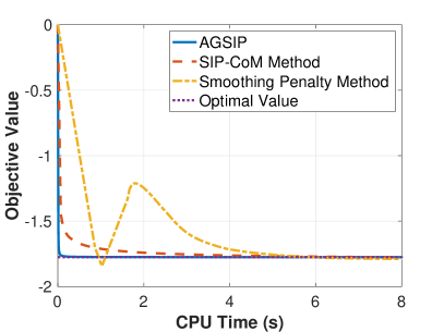
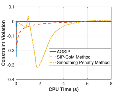
Figure 1: Convergence of objective values and constraint violations with CPU time.

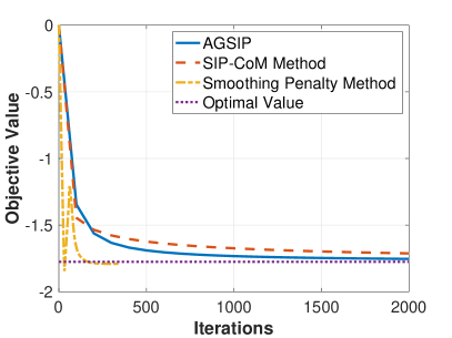
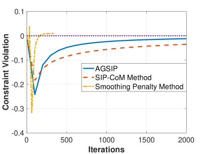
Figure 2: Convergence objective values and constraint violations with number of iterations.

9 Conclusions

Semi-infinite programming has applications in transportation, robotics, statistics and machine learning but it is challenging to solved due to the infinite number of constraints. Under the assumption of convexity, an effective primal-dual gradient method is proposed where, in each iteration, momentum-driven gradient ascend and descend steps are performed. This approach is also extended using stochastic gradient and function oracles, allowing it to solve large-scale data-driven problems through data sampling. The iteration complexity of the proposed method for finding an $\epsilon$-optimal solution is establish under different strong convexity assumptions, encompassing both deterministic and stochastic cases.

References

Adelman (2004)
D. Adelman.
A price-directed approach to stochastic inventory/routing.
Operations Research, 52(4):499–514, 2004.
Adelman (2007)
D. Adelman.
Dynamic bid prices in revenue management.
Operations Research, 55(4):647–661, 2007.
Adelman and Barz (2013)
D. Adelman and C. Barz.
A unifying approximate dynamic programming model for the economic lot scheduling problem.
Mathematics of Operations Research, 39(2):374–402, 2013.
Adelman and Klabjan (2012)
D. Adelman and D. Klabjan.
Computing near-optimal policies in generalized joint replenishment.
INFORMS Journal on Computing, 24(1):148–164, 2012.
Adelman and Mersereau (2013)
D. Adelman and A. Mersereau.
Dynamic capacity allocation to customers who remember past service.
Management Science, 59(3):592–612, 2013.
Betrò (2004)
Bruno Betrò.
An accelerated central cutting plane algorithm for linear semi-infinite programming.
Mathematical Programming, 101(3):479–495, 2004.
Boob et al. (2022)
Digvijay Boob, Qi Deng, and Guanghui Lan.
Stochastic first-order methods for convex and nonconvex functional constrained optimization.
Mathematical Programming, pages 1–65, 2022.
Calafiore and Campi (2005)
Giuseppe Calafiore and M. C. Campi.
Uncertain convex programs: randomized solutions and confidence levels.
Mathematical Programming, 102(1):25–46, 2005.
Cerulli et al. (2022)
Martina Cerulli, Antoine Oustry, Claudia d’Ambrosio, and Leo Liberti.
Convergent algorithms for a class of convex semi-infinite programs.
SIAM Journal on Optimization, 32(4):2493–2526, 2022.
Chambolle and Pock (2011)
Antonin Chambolle and Thomas Pock.
A first-order primal-dual algorithm for convex problems with applications to imaging.
Journal of mathematical imaging and vision, 40:120–145, 2011.
Chambolle and Pock (2016)
Antonin Chambolle and Thomas Pock.
On the ergodic convergence rates of a first-order primal–dual algorithm.
Mathematical Programming, 159(1-2):253–287, 2016.
Conn and Gould (1987)
Andrew R Conn and Nicholas IM Gould.
An exact penalty function for semi-infinite programming.
Mathematical Programming, 37(1):19–40, 1987.
Coope and Watson (1985)
Ian D Coope and G Alistair Watson.
A projected lagrangian algorithm for semi-infinite programming.
Mathematical Programming, 32(3):337–356, 1985.
Dall’Aglio (2001)
Marco Dall’Aglio.
On some applications of lsip to probability and statistics.
In Semi-infinite Programming, pages 237–254. Springer, 2001.
de Farias and Van Roy (2003)
D. P. de Farias and B. Van Roy.
The linear programming approach to approximate dynamic programming.
Operations Research, 51(6):850–865, 2003.
Dentcheva and Ruszczyński (2004)
Darinka Dentcheva and Andrzej Ruszczyński.
Semi-infinite probabilistic optimization: first-order stochastic dominance constrain.
Optimization, 53(5-6):583–601, 2004.
Fang et al. (2001)
Shu-Cherng Fang, Chih-Jen Lin, and Soon-Yi Wu.
Solving quadratic semi-infinite programming problems by using relaxed cutting-plane scheme.
Journal of computational and applied mathematics, 129(1):89–104, 2001.
Farias and Van Roy (2007)
V. F. Farias and B. Van Roy.
An approximate dynamic programming approach to network revenue management.
Working paper, Stanford Univ., 2007.
Ferris and Philpott (1989)
Michael C Ferris and Andrew B Philpott.
An interior point algorithm for semi-infinite linear programming.
Mathematical Programming, 43(1):257–276, 1989.
Goberna and Lopez (2002)
Miguel A Goberna and Marco A Lopez.
Linear semi-infinite programming theory: An updated survey.
European Journal of Operational Research, 143(2):390–405, 2002.
Goberna and López (2013)
Miguel Ángel Goberna and Marco A López.