Higher-order protection of quantum gates: Hamiltonian engineering
coordinated with dynamical decoupling

Abstract

Dynamical decoupling represents an active approach towards the protection of quantum memories and quantum gates. Because dynamical decoupling operations can interfere with system’s own time evolution, the protection of quantum gates is more challenging than that of quantum states. In this work, we put forward a simple but general approach towards the realization of higher-order protection of quantum gates. The central idea of our approach is to engineer (hence regain the control of) the quantum gate Hamiltonian in coordination with higher-order dynamical decoupling sequences originally proposed for the protection of quantum memories. In our computational examples presented for illustration, the required engineering can be implemented by only quenching the phase of an external driving field at particular times.

Introduction.— A crucial challenge in implementing quantum computation is to overcome the decoherence induced by the interaction between a quantum system and its environment. As an active approach, dynamical decoupling (DD) aims to average out system-environmental interaction and hence protects either quantum memories or quantum gates Viola ; Viola1999 . For quantum memories, periodic DD (PDD) Viola2003 eliminates the effect of system-environment interaction to the first-order (e.g., in the sense of a Magnus expansion), whereas concatenated DD (CDD) Khodjasteh and Uhrig DD (UDD) Uhrig ; Yang ; West2010 can offer higher-order elimination of decoherence Gong ; Gong2010 . Experimental advances on DD-based quantum memory protection have been highly successful Biercuk ; Du ; Ryan ; deLange ; Wang ; Alvarez , with recent benchmarking studies of DD carried out on actual noisy quantum computers Ezzell . However, most of these experimental progresses on quantum memory protection have not been translated to the protection of quantum gates, because DD operations often interfere with quantum gate operations, e.g., DD pulses tend to freeze system’s own time evolution.

One solution towards the DD protection of quantum gates started with certain driving Hamiltonian commutable with DD operations Byrd ; Lidar2008 ; West , the so-called “non-interference” condition. This stimulating route however needs extra physical qubit resources to encode logical qubits, the implementation of which is often based on particular dynamical symmetries or specific physical interactions to meet the non-interference requirement Xu ; Zhao ; Wu . The second solution utilizes gate operations inserted in between DD pulses. This approach typically extends the total gate time and can only realize first-order protection Suter ; Zhang ; Souza . To further fill in the gap between quantum memory protection and quantum gate protection by DD, the dynamically corrected gate (DCG) was proposed as a sophiticated composite quantum gate constructed from primitive building blocks without encoding Viola2009 ; ViolaPRA ; Ng . DCG may offer higher-order protection with concatenate design Viola2010 , but the total number of the required gate operations will be large and thus experimentally challenging. It remains to see if it is possible to reduce the overhead in the realization of higher-order protection of quantum gates.

This work aims to show that higher-order protection of quantum gates can be directly achieved on general physical qubits, with straightforward driving Hamiltonians that are piecewise continuous and at no cost of the total gate time. The central idea of our higher-order approach lies in the engineering of the time dependence of system’s driving Hamiltonian Viola2003 , in coordination with higher-order DD sequences originally designed for quantum memory protection, such as CDD, UDD, and even nested UDD. Because the realization of DD pulses already requires to design explicit and rapid time dependence of system’s Hamiltonian, engineering some additional time dependence of system’s driving Hamiltonian does not present a challenge when compared with the task of qubit encoding. As seen below, the required engineering of system’s driving Hamiltonian is to act against the unwanted impact of DD pulses on the system. This being done, only the system-environment interaction part is suppressed to higher orders and we recover our control over system’s driving Hamiltonian. The DD protection of quantum memories and quantum gates can thus be unified and applied on an equal footing. Our theoretical proposal is verified by our computational examples below.

Approach.— Consider a quantum system coupled to its environment with the total Hamiltonian $H(t)=H_{\rm S}(t)+H_{\rm E}+H_{\rm I}$. Here, $H_{\rm S}(t)$ is our system’s driving Hamiltonian, $H_{\rm E}$ is the environment Hamiltonian and $H_{\rm I}$ is the system-environment interaction. The most general interaction between a qubit and its environment is in the form $H_{\rm I}=\sigma_{x}\otimes{E_{x}}+\sigma_{y}\otimes{E_{y}}+\sigma_{z}\otimes{E_{z}}$, where ${E}_{x(y,z)}$ represent the associated environment operators. To illustrate the underlying principle of our idea, we start with a one-qubit case under PDD pulses, where

$$H_{\rm S}(t)=\Omega_{x}(t)\sigma_{x}+\Omega_{y}(t)\sigma_{y},$$ (1)

with $\Omega_{x}(t)$ and $\Omega_{y}(t)$ being time-dependent system parameters.

Let us now consider a periodic sequence of fast and strong symmetrizing pulses with the DD operations $\{\sigma_{0},\sigma_{1},\sigma_{2},\sigma_{3}\}$ ($\sigma_{0}\equiv{I}$, $\sigma_{1}\equiv{\sigma_{x}}$, $\sigma_{2}\equiv{\sigma_{y}}$ and $\sigma_{3}\equiv{\sigma_{z}}$ with $I$ corresponding to no pulse applied), over a duration of $4\tau$, applied to the native evolution governed by the driving Hamiltonian $H_{\rm S}(t)$. Assuming that the applied pulses are instantaneous (that is, much shorter than the total gate time $4\tau$), the time evolution operator is given by

$$\mathcal{U}= \prod^{3}_{k=0}\sigma_{k}\mathcal{T}e^{-i\int^{(k+1)\tau}_{k\tau}\mathcal{H}(t)dt}\sigma_{k}$$

$$= \prod^{3}_{k=0}\mathcal{T}e^{-i\left[\int^{(k+1)\tau}_{k\tau}\sigma_{k}H_{\rm S}(t)\sigma_{k}dt+\sigma_{k}H_{\rm I}\sigma_{k}\tau+H_{\rm E}\tau\right]}$$

$$= \prod^{3}_{k=0}\mathcal{T}e^{-i\int^{(k+1)\tau}_{k\tau}\sigma_{k}H_{\rm S}(t)\sigma_{k}dt}e^{-i\left(\sum^{3}_{l=0}\sigma_{l}H_{\rm I}\sigma_{l}+4H_{\rm E}\tau\right)}+\mathcal{O}(\tau^{2}),$$ (2)

where the term with the smallest $k$ is placed at the right most and $\mathcal{T}$ denotes the time ordering. Note that $\sum^{3}_{l=0}\sigma_{l}H_{\rm I}\sigma_{l}=0$, so we have

$$\mathcal{U}= \prod^{3}_{k=0}\mathcal{T}e^{-i\int^{(k+1)\tau}_{k\tau}\sigma_{k}H_{\rm S}(t)\sigma_{k}dt}{\otimes}e^{-i4H_{\rm E}\tau}+\mathcal{O}(\tau^{2}).$$ (3)

Clearly then, the first-order effect arising from $H_{\rm I}$ is eliminated. It is also seen that the time evolution of the quantum system is strongly influenced by the DD pulses. Indeed, during each time interval of duration $\tau$, the effective Hamiltonian [see the exponentials in Eq. (3)] is updated by the DD pulses.

We now unravel a key observation behind our Hamiltonian engineering approach. Denote the effective Hamiltonians altered by DD pulses associated with the time interval $[k\tau,(k+1)\tau]$ as $H_{k}(t)\equiv\sigma_{k}H_{\rm S}(t)\sigma_{k}$. Using Eq. (1), one obtains $H_{0}(t)=\Omega_{x}(t)\sigma_{x}+\Omega_{y}(t)\sigma_{y}$, $H_{1}(t)=\Omega_{x}(t)\sigma_{x}-\Omega_{y}(t)\sigma_{y}$, $H_{2}(t)=-\Omega_{x}(t)\sigma_{x}+\Omega_{y}(t)\sigma_{y}$, and $H_{3}(t)=-\Omega_{x}(t)\sigma_{x}-\Omega_{y}(t)\sigma_{y}$. To fight against these changes to the system Hamiltonian imposed by DD pulses, we can quench the parameters of $H_{\rm S}(t)$ during the respective time intervals. Specifically for $t\in[0,\tau]$, $\Omega_{x}(t)=\Omega(t)\cos\varphi$ and $\Omega_{y}(t)=\Omega(t)\sin\varphi$, for $t\in(\tau,2\tau]$, $\Omega_{x}(t)=\Omega(t)\cos\varphi$ and $\Omega_{y}(t)=-\Omega(t)\sin\varphi$, for $t\in(2\tau,3\tau]$, $\Omega_{x}(t)=-\Omega(t)\cos\varphi$ and $\Omega_{y}(t)=\Omega(t)\sin\varphi$, and finally, for $t\in(3\tau,4\tau]$, $\Omega_{x}(t)=-\Omega(t)\cos\varphi$ and $\Omega_{y}(t)=-\Omega(t)\sin\varphi$. This can be experimentally implemented because $\Omega(t)$ is identified as the Rabi frequency of the qubit Hamiltonian and $\varphi$ represents a phase of the driving field coupling the two levels of the qubit. The proposed quenching can be realized by simply adjusting the phase parameter of the driving field, namely, the phase parameter should be chosen to be $\varphi$ for $t\in(0,\tau]$, $-\varphi$ for $t\in(\tau,2\tau]$, $-\varphi+\pi$ for $t\in(2\tau,3\tau]$ and $\varphi+\pi$ for $t\in(3\tau,4\tau]$. With phase parameters quenched in this manner, one has $H_{k}(t)=\Omega(t)(\cos\varphi\sigma_{x}+\sin\varphi\sigma_{y})$. That is, the effective Hamiltonians appearing in the exponentials in Eq. (3) become the same Hamiltonian $\Omega(t)(\cos\varphi\sigma_{x}+\sin\varphi\sigma_{y})$. If we further require $\int^{4\tau}_{0}\Omega(t)dt=\theta/2$, Eq. (3) indicates

$$\mathcal{U}=e^{-i\theta(\cos\varphi\sigma_{x}+\sin\varphi\sigma_{y})/2}\otimes e^{-i4H_{E}\tau}+\mathcal{O}(\tau^{2}).$$ (4)

As such, to the first order of $\tau$, system-environment coupling is eliminated and yet we still implement a gate operation, namely, rotating the qubit along an axis in the $xy$ plane by angle $\theta$. Remarkably, this is achieved without requiring that $H_{\rm S}(t)$ commutes with the DD operations.

We are now ready to engineer the time dependence of the qubit Hamiltonian for higher-order protection of quantum gates. As an example, we consider the second-order protection of a quantum gate by CDD with two layers. To that end, we use the time evolution protected by the DD operations $\{\sigma_{0},\sigma_{1},\sigma_{2},\sigma_{3}\}$ as the basic building block and then nest it with a second layer of DD operations $\{\sigma_{0},\sigma_{1},\sigma_{2},\sigma_{3}\}$. In doing so, we examine how the time dependence of $H_{\rm S}(t)$ should be engineered. The evolution operator with two layers of DD operations is given by

$$\mathcal{U}= \prod^{3}_{m=0}\sigma_{m}\left[\prod^{3}_{k=0}\mathcal{T}e^{-i\int^{(k+1)\tau/4}_{k\tau/4}\sigma_{k}H_{\rm S}(t)\sigma_{k}dt}\right]\sigma_{m}\otimes{e^{-i4H_{E}\tau}}+\mathcal{O}(\tau^{3})$$

$$= \prod^{3}_{m=0}\prod^{3}_{k=0}\mathcal{T}e^{-i\int^{(k+1)\tau/4}_{k\tau/4}\sigma_{m}\sigma_{k}H_{\rm S}(t)\sigma_{k}\sigma_{m}dt}\otimes{e^{-i4H_{E}\tau}}+\mathcal{O}(\tau^{3}),$$ (5)

where all the terms in the product should be arranged from right to left with increasing $k$ or $m$. We can analogously define the function appearing in the exponential as the effective Hamiltonian $H_{mk}(t)\equiv\sigma_{m}\sigma_{k}H_{\rm S}(t)\sigma_{k}\sigma_{m}$, with the explicit form easily found by use of Eq. (1). Just like the previous example showcasing first-order protection, here we can also quench the phase parameter $\varphi$ without changing the Rabi frequency parameter $\Omega(t)$ during time intervals as well as subintervals such that $H_{mk}(t)=\Omega(t)(\cos\varphi\sigma_{x}+\sin\varphi\sigma_{y})$. With $\int^{4\tau}_{0}\Omega(t)dt=\theta/2$, we have

$$\mathcal{U}=e^{-i\theta(\cos\varphi\sigma_{x}+\sin\varphi\sigma_{y})/2}\otimes e^{-i4H_{E}\tau}+\mathcal{O}(\tau^{3}),$$ (6)

indicating that our one-qubit gate with second-order protection is achieved. It is straightforward to extend our approach to cases of higher-order protection of quantum gates by increasing the concatenation level of CDD.

Let us now turn to more efficient higher-order protection of single-qubit quantum gates, using the same qubit Hamiltonian $H_{\rm S}(t)$ introduced above. According to the UDD theory proposed for quantum memory protection, the pure dephasing term $\sigma_{z}\otimes{E_{z}}$ can be filtered by applying nonequidistant decoupling operator $\sigma_{x}$. Likewise, the longitudinal relaxation term $\sigma_{x}\otimes{E_{x}}+\sigma_{y}\otimes{E_{y}}$ can be suppressed by applying $\sigma_{z}$ operations at special UDD timings Uhrig ; Yang ; West2010 . Building upon this, in order to average out the general system-environmental interaction $H_{I}=\sigma_{x}\otimes{E_{x}}+\sigma_{y}\otimes{E_{y}}+\sigma_{z}\otimes{E_{z}}$, we apply $n$ decoupling operations $\sigma_{x}$ to the quantum system at times $t_{j}=4\tau\sin^{2}[j\pi/(2n+2)]$, and during each time interval $[t_{j-1},t_{j}]$, we further apply $n$ decoupling operations $\sigma_{z}$ at times $t^{j}_{k}=t_{j}\sin^{2}[k\pi/(2n+2)]$, where $j,\ k=1,...,n$ and $n$ is taken as an even number to facilitate our engineering approach. Such a nested UDD protocol yields the following time evolution operator:

$$\mathcal{U}= \mathcal{U}({4\tau-t_{n}})\prod^{n}_{j=1}\sigma_{x}\mathcal{U}(t_{j}-t_{j-1})$$

$$= \prod^{n+1}_{j=1}\sigma^{j-1}_{x}\mathcal{U}(t_{j}-t_{j-1})\sigma^{j-1}_{x}$$ (7)

where $t_{0}\equiv 0$, $t_{n+1}\equiv 4\tau$, all the terms in the product from right to left should have an increasing $j$, and $\mathcal{U}(t_{j}-t_{j-1})$, the unitary evolution operator associated with the interval $[t_{j-1},t_{j}]$, is expressed by the subinterval evolution operators as

$$\mathcal{U}(t_{j}-t_{j-1})= \mathcal{U}({t_{j}-t^{j}_{n}})\prod^{n}_{k=1}\sigma_{z}\mathcal{U}(t^{j}_{k}-t^{j}_{k-1})$$

$$= \prod^{n+1}_{k=1}\sigma^{k-1}_{z}\mathcal{U}(t^{j}_{k}-t^{j}_{k-1})\sigma^{k-1}_{z}$$ (8)

with $t^{j}_{0}\equiv t_{j-1}$ and $t^{j}_{n+1}\equiv t_{j}$ and all the terms in the product from right to left should have an increasing $k$. The UDD theory can guarantee that the effect of system-environment interaction is suppressed up to the $n$th order. That is,

$$\mathcal{U}= \prod^{n+1}_{j=1}\prod^{n+1}_{k=1}\mathcal{T}e^{-i\int^{t^{j}_{k}}_{t^{j}_{k-1}}\sigma^{j-1}_{x}\sigma^{k-1}_{z}H_{\rm S}(t)\sigma^{k-1}_{z}\sigma^{j-1}_{x}dt}$$

$$\otimes{e}^{-i4H_{E}\tau}+\mathcal{O}(\tau^{n+1}).$$ (9)

To find out how to engineer the time dependence of $H_{\rm S}(t)$, we define effective Hamiltonians $H^{j}_{k}(t)\equiv\sigma^{j-1}_{x}\sigma^{k-1}_{z}H_{\rm S}(t)\sigma^{k-1}_{z}\sigma^{j-1}_{x}$, i.e., those terms appearing in the exponentials in the equation above. Further using Eq. (1), one obtains $H^{j}_{k}(t)=(-1)^{k-1}\Omega_{x}(t)\sigma_{x}+(-1)^{k+j}\Omega_{y}(t)\sigma_{y}$, explicitly depicting the impact of our nested UDD operations on the system Hamiltonian. To combat against these unwanted changes to the system Hamiltonian, we can just adjust only the phase parameter of the qubit driving field, such that for $t\in[t^{j}_{k-1},t^{j}_{k}]$, $\Omega_{x}(t)=(-1)^{k-1}\Omega(t)\cos\varphi$ and $\Omega_{y}(t)=(-1)^{k+j}\Omega(t)\sin\varphi$. The evident outcome of this phase quenching approach is that all the effective Hamiltonians will be the same, namely, $H^{j}_{k}(t)=\Omega(t)(\cos\varphi\sigma_{x}+\sin\varphi\sigma_{y})$. Assuming $\int^{4\tau}_{0}\Omega(t)dt=\theta/2$, then one arrives at

$$\mathcal{U}=e^{-i\theta(\cos\varphi\sigma_{x}+\sin\varphi\sigma_{y})/2}\otimes e^{-i4H_{E}\tau}+\mathcal{O}(\tau^{n+1}),$$ (10)

which is a quantum gate protected by nested UDD to the $n$th order. To our knowledge, such a possibility of higher-order UDD protection of quantum gates is never shown before. In addition, the quantum gate time is still the same as in the bare case without protection. To see that more explicitly, let $\Omega$ be the average Rabi frequency during $[0,4\tau]$, namely, $\Omega=[\int^{4\tau}_{0}\Omega(t)dt]/(4\tau)$. Then for all the cases illustrated above, the total gate time $4\tau$ remains to be $\theta/(2\Omega)$.

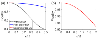
Figure 1: Quantum gate fidelity as a function of the system-environment coupling strength $\epsilon$. (a) Fidelity $F$ with the first-order protection (blue), second-order protection (red), and without protection (black) for $\epsilon\in[0,0.5\Omega]$. (b) More results of fidelity $F$ under the second-order protection with CDD for $\epsilon\in[0,2\Omega]$.

Numerical results.— To verify our engineering concept, let us consider a simple form of system-environment interaction of the following Heisenberg coupling form

$$H_{\rm I}=\epsilon(\sigma_{x}^{s}\sigma_{x}^{b}+\sigma_{y}^{s}\sigma_{y}^{b}+\sigma_{z}^{s}\sigma_{z}^{b}),$$ (11)

with the first spin represents the qubit Hamiltonian and the second spin represents a quantum bath, and $\epsilon$ being the coupling strength. We also assume that there is no driving field acting solely on the environment spin. Admittedly, this $H_{\rm I}$ is extremely simple as compared with a real quantum bath, but it does capture the essence that the qubit system is subject to both dephasing and population relaxation and it suffices to illustrate how our engineering approach leads to higher-order protection. $H_{\rm I}$ may also model some residue interaction between a qubit under gate operation and its surrounding qubit.

Table 1: Computational results of $[\epsilon,F_{\mathrm{bare}},F_{\mathrm{PDD}},F_{\mathrm{CDD}}]$, namely, quantum gate fidelity without protection, with first order PDD and second-order CDD vs the system-environment coupling strength $\epsilon$.

$\epsilon/\Omega$		$0.05$		$0.1$		$0.2$		$0.3$		$0.4$		$0.5$
$F_{\mathrm{bare}}$		$98.75\%$		$95.05\%$		81.47%		$63.57\%$		47.45%		$38.67\%$
$F_{\mathrm{PDD}}$		$99.90\%$		$99.61\%$		98.39%		$96.31\%$		93.37%		$89.60\%$
$F_{\mathrm{CDD}}$		$99.99\%$		$99.98\%$		$99.92\%$		$99.82\%$		99.67%		$99.49\%$

The performance of our higher-order protection is characterized by the fidelity $F=\langle\phi|\rho|\phi\rangle$. Here, $|\phi\rangle$ is the target output state and $\rho$ is the real output state that is obtained by first solving the Liouville equation $\dot{\varrho}(t)=-i[H(t),\varrho(t)]$ and then performing a partial trace over the environment spin. We take the initial state as $(|0\rangle+|1\rangle)/\sqrt{2}$, the parameters of the driving Hamiltonian as $\Omega=10\pi\ \mathrm{MHz}$ and $\varphi=\pi/4$, and the evolution time as $0.05\mathrm{\mu{s}}$. The ideal quantum gate under these choices are hence $U=(\sigma_{x}+\sigma_{y})/\sqrt{2}$ and the target output state is $|\phi\rangle=[\exp(-i\pi/4)|0\rangle+\exp(i\pi/4)|1\rangle]/\sqrt{2}$. To illustrate how higher-order protection can be achieved, we tune the system-environment coupling strength $\epsilon$ over a wide range, namely, $\epsilon\in[0,0.5\Omega]$. We then plot the fidelity $F$ vs the coupling strength $\epsilon$ for the quantum gate under PDD and CDD with first-order and second-order protection, as shown by the blue and red lines in Fig. 1(a). As a comparison, we also plot the gate fidelity without any DD protection, as shown by the black line in Fig. 1(a).

Figure 1 illustrates that while the first-order protection yields gate fidelities much better than that of the bare gate, the second-order protection further dramatically improves the performance of the quantum gate. In particular, for the worse case $\epsilon=2\Omega$ (the system-bath coupling strength is twice of the Rabi frequency), the gate fidelity with second-order protection can still reach more than $92\%$, shown in Fig. 1(b). To appreciate the DD improvement more quantitatively, we present in table 1 our computational findings based on our simple model. As seen from table 1 , for a moderate coupling strength $\epsilon=0.05\Omega$, the gate fidelities under first-order and second-order protection can reach $F_{\mathrm{PDD}}=99.90\%$ and $F_{\mathrm{CDD}}=99.99\%$, respectively, both being much higher than the fidelity $F_{\mathrm{bare}}=98.75\%$ without DD protection. Notably, for the case $\epsilon=0.5\Omega$, i.e., the coupling strength is approximately half of the Rabi frequency of gate Hamiltonian such that the fidelity of the bare gate is as low as $38.67\%$ (the gate is basically totally destroyed), the first-order protection can boost the fidelity back to $90\%$ (which may not suffice for an actual quantum computation application), but the second-order protection can further improve the fidelity to $99.49\%$. These numerical findings do not represent at all what one can achieve on an actual quantum computing platform, but indicating the promise of higher-order protection of gate operations, now made possible by our engineering approach.

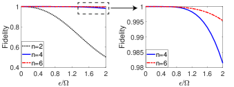
Figure 2: Quantum gate fidelity as a function of the system-environment coupling strength over a wide range of $\epsilon\in[0,2\Omega]$ under nested UDD protection. Black, blue and red lines respectively correspond to the protection under the orders of $n=2$, $4$ and $6$.

Next let us check the performance of our approach when using nested UDD to protect the quantum gate to the $n$th order according to our protocol outlined above. Figure 2 presents the corresponding gate fidelity for a wide range of $\epsilon\in[0,2\Omega]$, with $n=2$, $4$ and $6$. The gate fidelity is seen to be greatly enhanced when we increase the order of protection. We further present our numerics in table 2. As seen from table 2, for $\epsilon\in[0,2\Omega]$, the gate fidelity with $4$th and $6$th protection always exceed $98\%$. Remarkably, the fidelity with $6$th order protection can be as high as $99.54\%$ even when the system-environment coupling strength is twice of the Rabi frequency of the system Hamiltonian.

Table 2: Computational results of $[\epsilon,F_{\rm UDD-2},F_{\rm UDD-4},F_{\rm UDD-6}]$, namely, quantum gate fidelity under second-order, fourth-order, and sixth-order UDD protection vs the system-environment coupling strength $\epsilon$, with a nested UDD scheme.

$\epsilon/\Omega$		$0.2$		$0.6$		$1.0$		$1.4$		$2.0$
$F_{\rm UDD-2}$		$99.57\%$		$94.96\%$		$84.51\%$		70.18%		$50.28\%$
$F_{\rm UDD-4}$		$99.9998\%$		$99.995\%$		$99.93\%$		99.63%		$98.14\%$
$F_{\rm UDD-6}$		$99.9999\%$		$99.996\%$		$99.97\%$		99.88%		$99.54\%$

Two-qubit gates.— Having computationally verified that the concept underlying our engineering approach is valid, we finally discuss how to protect a nontrivial two-qubit gate, which is important for universal quantum computation under DD protection. As an example, we show below how to engineer a two-qubit Hamiltonian to realize a nontrivial two-qubit gate under second-order protection. Let us now start to consider a system Hamiltonian different from all single-qubit cases discussed above, namely,

$$H_{\rm S}=J_{1}(t)\sigma_{z}^{(1)}+J_{2}(t)\sigma_{z}^{(2)}+J(t)\sigma_{z}^{(1)}\otimes\sigma_{z}^{(2)},$$ (12)

where $J_{1}$ and $J_{2}$ are the parameters of local operations respectively acting on the first and second qubits, and $J$ is the coupling parameter between the two qubits. We assume each qubit is subject to its own dephasing and population relaxation. To suppress the decoherence to the second order, we exploit the time evolution protected by the PDD operations $\{\sigma_{0}^{(1)}\otimes\sigma_{0}^{(2)},\sigma_{1}^{(1)}\otimes\sigma_{1}^{(2)},\sigma_{2}^{(1)}\otimes\sigma_{2}^{(2)},\sigma_{3}^{(1)}\otimes\sigma_{3}^{(2)}\}$ as the basic building block and then nest it into a second layer of the same DD operations. As a result, the time evolution operator over a period of $4\tau$ is found to be

$$\mathcal{U}= \Bigg{[}\prod^{3}_{m=1}\sigma_{m}^{(1)}\otimes\sigma_{m}^{(2)}\prod^{3}_{k=1}\mathcal{T}e^{-i\int^{(k+1)\tau/4}_{k\tau/4}\sigma_{k}^{(1)}\otimes\sigma_{k}^{(2)}H_{\rm S}(t)\sigma_{k}^{(1)}\otimes\sigma_{k}^{(2)}dt}$$

$$\times\sigma_{m}^{(1)}\otimes\sigma_{m}^{(2)}\Bigg{]}\otimes{e^{-i4H_{E}\tau}}+\mathcal{O}(\tau^{3})$$

$$= \prod^{3}_{m=1}\prod^{3}_{k=1}\mathcal{T}e^{-i\int^{(k+1)\tau/4}_{k\tau/4}\sigma_{m}^{(1)}\sigma_{k}^{(1)}\otimes\sigma_{m}^{(2)}\sigma_{k}^{(2)}H_{\rm S}(t)\sigma_{k}^{(1)}\sigma_{m}^{(1)}\otimes\sigma_{k}^{(2)}\sigma_{m}^{(2)}dt}$$

$$\otimes{e^{-i4H_{E}\tau}}+\mathcal{O}(\tau^{3}),$$ (13)

Again we may define the effective Hamiltonians $H_{mk}(t)\equiv[\sigma_{m}^{(1)}\sigma_{k}^{(1)}]\otimes[\sigma_{m}^{(2)}\sigma_{k}^{(2)}]H_{\rm S}(t)[\sigma_{k}^{(1)}\sigma_{m}^{(1)}]\otimes[\sigma_{k}^{(2)}\sigma_{m}^{(2)}]$. Using the expression of such effective Hamiltonians, it can be observed that the impact of DD pulses on the system Hamiltonian will not flip the sign of the qubit-qubit interaction term $J(t)\sigma_{z}^{(1)}\otimes\sigma_{z}^{(2)}$. In other words, only the sign of the single-qubit terms $J_{1}(t)\sigma_{z}^{(1)}$ and $J_{2}(t)\sigma_{z}^{(2)}$ may be changed. When this change does occur, we can just reverse the direction of the driving field to cancel the unwanted action of the CDD pulses. As an example where $|J_{1}(t)|=|J_{2}(t)|=J(t)$, our quench protocol coordinated with DD pulses will lead to $H_{mk}=-J(t)[\sigma^{(1)}_{z}+\sigma^{(2)}_{z}-\sigma^{(1)}_{z}\sigma^{(2)}_{z}]$. For $\int^{4\tau}_{0}J(t)dt=\theta/2$, we obtain

$$\mathcal{U}=e^{-i\theta(\sigma_{z}^{(1)}\otimes{I}+{I}\otimes\sigma_{z}^{(2)}-\sigma_{z}^{(1)}\sigma_{z}^{(2)})/2}\otimes e^{-i4H_{E}\tau}+\mathcal{O}(\tau^{3}).$$ (14)

Ignoring an unimportant global phase factor $\exp(-i\theta/2)$, this gate under second-order protection yields

$$U=|00\rangle\langle 00|+|01\rangle\langle 01|+|10\rangle\langle 10|+e^{i\theta}|11\rangle\langle 11|,$$ (15)

which is a controlled-phase gate. Combined with protected single-qubit gates illustrated above, we have thus conceptually shown that in principle it is possible to execute universal quantum computation under higher-order protection with Hamiltonian engineering.

Discussions.— We have proposed a simple approach towards the realization of higher-order protection of quantum gates. The central idea is to quench a gate Hamiltonian to combat against the influence of DD pulses on the time evolution of the system. This way, on the one hand we manipulate the quantum states by DD to average out system-bath interaction to high orders; on the other hand we regain our control on quantum evolution and hence achieve high-order protection of quantum gates. This work thus indicates that highly efficient schemes such as UDD for quantum memory protection can be integrated with quantum gates with higher-order protection. Though in this work we only illustrated our idea using general-purpose PDD, CDD and UDD sequences, our approach can exploit other DD designs as well. In particular, if there is spectral information about the environment noise, then the time intervals between DD sequences can be further optimized according to the noise spectrum Gong11 and as a result, quantum gate protection using our concept can directly benefit from such optimization that can further drastically improve the performance of decoherence suppression. Our Hamiltonian engineering approach in coordination with DD hence makes the measurement of environment spectrum much more relevant than before to the realization of high-fidelity quantum gates. Numerics presented in this work are not aimed to simulate a realistic situation, but to verify that our approach is conceptually correct. Indeed, as a price to implement our design, we have assumed instantaneous DD control pulses as compared with the total gate time. It will be of great interest to examine the actual performance of our simple design on real physical platforms, including noisy intermediate scale quantum computers.

Acknowledgments.— J.G. is grateful to Lorenza Viola for technical discussions and for her highly constructive comments on the first version of our manuscript. This work was supported by the National Research Foundation, Singapore and A*STAR under its CQT Bridging Grant.

References

- (1) L. Viola, E. Knill, and S. Lloyd, Phys. Rev. Lett. 82, 2417 (1999).
- (2) L. Viola, S. Lloyd, and E. Knill, Phys. Rev. Lett. 83, 4888 (1999).
- (3) L. Viola and E. Knill, Phys. Rev. Lett. 90, 037901 (2003).
- (4) K. Khodjasteh and D. A. Lidar, Phys. Rev. Lett. 95, 180501 (2005).
- (5) G. S. Uhrig, Phys. Rev. Lett. 98, 100504 (2007).
- (6) W. Yang and R. B. Liu, Phys. Rev. Lett. 101, 180403 (2008).
- (7) J. R. West, B. H. Fong, and D. A. Lidar, Phys. Rev. Lett. 104, 1130501 (2010).
- (8) M. Mukhtar, T. B. Saw, W. T. Soh, and J. Gong, Phys. Rev. A 81, 012331 (2010).
- (9) M. Mukhtar, W. T. Soh, T. B. Saw, and J. Gong, Phys. Rev. A 82, 052338 (2010).
- (10) M. J. Biercuk, H. Uys, A. P. VanDevender, N. Shiga, W. M. Itano, and J. J. Bollinger, Nature 458, 996 (2009).
- (11) J. F. Du, X. Rong, N. Zhao, Y. Wang, J. H. Yang, and R. B. Liu, Nature 461, 1265 (2009).
- (12) C. A. Ryan, J. S. Hodges, and D. G. Cory, Phys. Rev. Lett. 105, 200402 (2010).
- (13) G. deLange, Z. H. Wang, D. Risté, V. V. Dobrovitski, and R. Hanson, Science 330, 60 (2010).
- (14) Y. Wang, X. Rong, P. B. Feng, W. J. Xu, B. Chong, J. H. Su, J. Gong, and J. F. Du, Phys. Rev. Lett. 106, 040501 (2011).
- (15) G. A. Álvarez, A. M. Souza, and D. Suter, Phys. Rev. A 85, 052324 (2012).
- (16) N. Ezzell, B. Pokharel, L. Tewala, G. Quiroz, and D. A. Lidar, arXiv: 2207.03670.
- (17) M. S. Byrd and D. A. Lidar, Phys. Rev. Lett. 89, 047901 (2002).
- (18) D. A. Lidar, Phys. Rev. Lett. 100, 160506 (2008).
- (19) J. R. West, D. A. Lidar, B. H. Fong, and M. F. Gyure, Phys. Rev. Lett. 105, 230503 (2010).
- (20) G. F. Xu and G. L. Long, Phys. Rev. A 90, 022323 (2014).
- (21) P. Z. Zhao , X. Wu, and D. M. Tong, Phys. Rev. A 103, 012205 (2021).
- (22) C. F. Wu, C. F. Sun, J. L. Chen, and X. X. Yi , Phys. Rev. Appl. 19, 034069 (2023).
- (23) A. M. Souza, G. A. Álvarez, and D. Suter, Phys. Rev. A 86, 050301(R) (2012).
- (24) J. F. Zhang, A. M. Souza, F. D. Brandao, and D. Suter, Phys. Rev. Lett. 112, 050502 (2014).
- (25) D. Suter and G. A. Álvarez, Rev. Mod. Phys. 88, 041001 (2016).
- (26) K. Khodjasteh and L. Viola, Phys. Rev. Lett. 102, 080501 (2009).
- (27) K. Khodjasteh and L. Viola, Phys. Rev. A 80, 032314 (2009).
- (28) H. K. Ng, D. A. Lidar, and J. Preskill , Phys. Rev. A 84, 012305 (2011).
- (29) K. Khodjasteh, D. A. Lidar, and L. Viola, Phys. Rev. Lett. 104, 090501 (2010).
- (30) Y. Pan, Z. R. Xi, and J. Gong, J. Phys. B 44, 175501 (2011).