WGoM: A novel model for categorical data with weighted responses

Abstract

The Graded of Membership (GoM) model is a powerful tool for inferring latent classes in categorical data, which enables subjects to belong to multiple latent classes. However, its application is limited to categorical data with nonnegative integer responses, making it inappropriate for datasets with continuous or negative responses. To address this limitation, this paper proposes a novel model named the Weighted Grade of Membership (WGoM) model. Compared with GoM, our WGoM relaxes GoM’s distribution constraint on the generation of a response matrix and it is more general than GoM. We then propose an algorithm to estimate the latent mixed memberships and the other WGoM parameters. We derive the error bounds of the estimated parameters and show that the algorithm is statistically consistent. The algorithmic performance is validated in both synthetic and real-world datasets. The results demonstrate that our algorithm is accurate and efficient, indicating its high potential for practical applications. This paper makes a valuable contribution to the literature by introducing a novel model that extends the applicability of the GoM model and provides a more flexible framework for analyzing categorical data with weighted responses.

1 Introduction

Many systems take the form of categorical data: sets of subjects (individuals) and items joined together by categorical responses. Categorical data are widely collected across diverse fields such as social science, psychological science, behavioral science, biological science, and transportation[1, 2, 3, 4, 5, 6, 7, 8, 9, 10, 11]. Categorical data usually has a finite number of values, where each value represents an outcome from a finite number of possible choices like age group, educational level, and preference level.

Categorical data can be represented mathematically using a $N$-by-$J$ response matrix $R$, where $N$ indicates the number of subjects and $J$ indicates the number of items. Each element $R(i,j)$ constitutes the observed response of the $i$-th subject to the $j$-th item. When the response is binary, the elements of $R$ are either 0 or 1. The binary responses can be agree/disgree (or yes/no) responses in a psychological test, correct/wrong responses in an educational assessment, spam/legitimate emails in an email classification project, and so on. When the response is categorical, the elements of $R$ are commonly non-negative integers. The categorical responses can be different types of accommodation such as house/condominium/apartment in an accommodation recommendation, different strengths of agreement such as strongly disagree/disagree/moderate/agree/strongly agree in a psychological test, and so on. Additional examples of categorical data can be found in Agresti’s book [5].

Based on categorical data, researchers in the aforementioned fields are typically interested in identifying latent classes (i.e., underlying groups) of subjects such that subjects within the same class share similar characteristics [12, 13, 14, 15, 16, 17]. For example, latent classes may represent different types of mental states like schizophrenia/depression/neurosis/normal in a mental disorder test, different ability levels like high/medium/low/basic/unqualified levels in an educational assessment, different political ideologies like liberal/neutral/conservative parties in a political survey, and different types of personalities like openness/conscientiousness/extraversion/agreeableness/neuroticism in a psychological test.

Latent class model (LCM) [18] is a popular statistical model used for identifying latent classes for categorical data in the aforementioned fields. In recent years, Bayesian inference techniques [19, 20, 21, 22], maximum likelihood estimation (MLE) methods [23, 24, 25, 26], and tensor-based algorithms [27, 28] are used to estimate latent classes for data generated from LCM. One main limitation of LCM is, it assumes that each subject belongs to a single class and there is no overlap between different classes. However, for most real-world data, a subject may belong to multiple classes. For example, a conscientiousness subject in a psychological test may also be openness; a neutral subject in a political survey can be thought of having mixed memberships such that it belongs to liberal class and conservative class simultaneously but with different weights for each class when we assume that there are two latent classes [29]. The Grade of Membership (GoM) model [30] was proposed as a generalization of LCM by allowing each subject to belong to more than one classes. GoM is also known as ‘admixture’ or ‘topic’ or Latent Dirichlet Allocation model [31, 32, 33, 34, 35, 36]. GoM assumes that each subject has a membership vector (i.e., probability mass function) that sums to one. The $k$-th value of the membership vector denotes the probability (i.e., extent) that a subject partially belongs to the $k$-th class. Thus, GoM is more flexible than LCM. Bayesian inference methods [37, 38, 39], MLE approach [40], variational Expectation-Maximization algorithm [41], and spectral method [42] are designed to infer the latent mixed memberships for data generated from GoM. A detailed comparison between GoM and LCM can be found in [43].

Unfortunately, the Grade of Membership model mentioned above has a significant limitation: it only functions for categorical data with binary responses or non-negative integer responses, and it is not applicable to data with weighted responses, where the responses can be continuous or even negative. Such data is frequently collected in real-world situations and ignoring weighted responses may result in losing potentially valuable information about the unobserved structures [44]. For example, in the Wikipedia elections data [45], which is a dataset of users from the English Wikipedia that voted for or against each other in admin elections, both subjects and items represent individual users, and the responses can be positive (i.e., voted for) and negative (i.e., voted against), i.e., each element of $R$ is either -1 or 1 (we call such $R$ signed response matrix in this paper). In the trust data of Advogato [46], both subjects and items represent users of the online community platform Advogato, and the responses represent trust relationships with three different levels: apprentice (0.6), journeyer (0.8), and master (1), i.e., each element of $R$ ranges in $\{0.6,0.8,1\}$. In Jester 100 [47], which is a dataset records information about how users rated a total amount of 100 jokes, subjects are users and items represent jokes, and the rating values are continuous values between $-10$ and $10$, i.e., each entry of $R$ ranges in $[-10,10]$. In Bitcoin Alpha [48], which is a user-user trust/distrust dataset from the Bitcoin Alpha platform, the responses represent trust or distrust on a scale from $-10$ to 10, i.e., all elements of $R$ range in $\{-10,-9,-8,\ldots,8,9,10\}$. In Dutch college [49], which is a dataset records ratings of friendship between 32 university freshmen, the responses range from $-1$ for risk of getting into conflict to 3 for best friend, i.e., the elements of $R$ take value in $\{-1,0,1,2,3\}$. In the FilmTrust ratings data [50], subjects (users) rate items (films), and the responses (ratings) range in $\{0.5,1,1.5,2,2.5,3,3.5,4\}$. These datasets are collected by [51] and can be obtained from the following URL link: http://konect.cc/networks/. GoM fails to model all the aforementioned data with weighted responses. Therefore, it is desirable to develop a more general and more flexible statistical model for weighted response data, where the responses can be continuous and negative. With this motivation, the present paper executes the following key advancements:

• To model categorical data with weighted responses, we propose a novel generative model, the Weighted Grade of Membership (WGoM) model. It achieves the goal to model weighted response categorical data by allowing the observed response matrix $R$ to be generated from an arbitrary distribution provided that the expectation of $R$ enjoys a structure reflecting the membership of each subject. For example, under WGoM, $R$ with a latent class structure can be generated from Bernoulli, Binomial, Poisson, Uniform, and Normal distributions, etc. Especially, any observed response matrix $R$ with a finite number of distinct elements, where the responses can be any real value, can be modeled by our WGoM, and this is guaranteed by our Theorem 1. Compared with GoM, our model WGoM releases GoM’s distribution restriction on $R$ and GoM is a special case of our WGoM.

• To facilitate a broad application of our model WGoM, we propose an efficient and easy-to-implement method for estimating subjects’ memberships and the other WGoM parameters. We derive the theoretical convergence rates of our method and show that the method yields consistent estimation. We also provide some instances for further analysis and find that our method may behave differently when the observed response matrices are generated from different distributions under WGoM.

• To verify our theoretical analysis and assess the accuracy and effectiveness of the proposed method, we conduct extensive experiments and apply our method to a real-world test data with meaningful results.

1.1 Notation and organization

The following notations will be used throughout this paper. For any positive integer $m$, we denote $[m]=\{1,2,\ldots,m\}$ and define $I_{m\times m}$ as the $m\times m$ identity matrix. For any scale $a$, $|a|$ denotes its absolute value. For any vector $x$, $x^{\prime}$ denotes its transpose and $\|x\|_{q}$ denotes its $l_{q}$-norm for any $q>0$. For any matrix $M$, we use $M^{\prime},M(i,:),M(:,j),M(i,j),M(S,:),M^{-1},\|M\|,\|M\|_{F},\|M\|_{2\rightarrow\infty},\mathrm{rank}(M),\sigma_{k}(M),\lambda_{k}(M),\kappa(M)$, and $\mathrm{max}(0,M)$ to denote its transpose, $i$-th row, $j$-th column, $ij$-th entry, submatrix formed by rows in the set $S$, inverse when $M$ is nonsingular, spectral norm, Frobenius norm, maximum $l_{2}$-norm among all rows, rank, $k$-th largest singular value, $k$-th largest eigenvalue ordered by magnitude when $M$ is a square matrix, conditional number, and nonnegative part, respectively. Here, $\|M\|=\sigma_{1}(M),\|M\|_{F}=\mathrm{trace}(M^{\prime}M)$ (i.e., the trace of the square matrix $M^{\prime}M$), and $\|M\|_{2\rightarrow\infty}=\mathrm{max}_{i}\|M(i,:)\|_{2}$. Let notations $\mathbb{R}$ and $\mathbb{N}$ denote the sets of real numbers and nonnegative integers, respectively. For any random variable $Y$, $\mathbb{E}(Y)$ denotes its expectation and $\mathbb{P}(Y=a)$ denotes the probability that $Y$ equals to $a$. Let $\mathcal{X}^{n\times m}$ denote the space of all $n\times m$ matrices, whose entries are taken from the set $\mathcal{X}$. $e_{i}$ represents a vector whose $i$-th entry is 1 and all the others entries are 0.

The rest of this paper is organized as follows. In Section 2, we formally introduce our model and demonstrate its generality and identifiability. In Section 3, we propose the algorithm, explain its rationality, and provide its computational complexity. In Section 4, we establish the theoretical result and explain its generality by providing several instances. Sections 5-6 contain the numerical and empirical results, respectively. Section 7 concludes this paper with a discussion. Detailed technical proofs and extra instances are included in the Appendix.

2 Weighted Grade of Membership model

In the weighted response setting presented in this paper, let $R\in\mathbb{R}^{N\times K}$ be the observed weighted response matrix, such that $R(i,j)$ denotes the weighted response of subject $i$ to the $j$-th item for all $i\in[N],j\in[J]$. Here, the response $R(i,j)$ can take any real value in our weighted response setting.

Our Weighted Grade of Membership (WGoM) model can be described by two modeling facets: the population aspect and the individual aspect. On the population aspect, WGoM assumes that there are $K$ latent classes that describe response patterns. Throughout this paper, the number of latent classes, $K$, is assumed to be known. Let $\Theta\in\mathbb{R}^{J\times K}$ be the item parameter matrix, with elements that can take any real value. To render our model identifiable, we require $\mathrm{rank}(\Theta)=K$. For $k\in[K]$, our model WGoM assumes that $\Theta(j,k)$ captures the conditional response expectations under an arbitrary distribution $\mathcal{F}$. Specifically, for $j\in[J],k\in[K],$ WGoM assumes Equation (1) below holds under an arbitrary distribution $\mathcal{F}$.

$$\mathbb{E}(R(i,j)|\mathrm{subject~{}}i~{}\mathrm{belongs~{}to~{}the~{}}k\mathrm{-th~{}latent~{}class})=\Theta(j,k).$$ (1)

On the individual aspect, since a subject may belong to multiple latent classes with different weights in this paper, we let $\Pi$ be the $N\times K$ membership matrix such that $\Pi(i,k)$ denotes the extent that $i$-th subject partially belongs to the $k$-th latent class for $i\in[N],k\in[K]$. $\Pi$ is assumed to satisfy the following conditions:

$$\Pi(i,k)\geq 0,\sum_{l=1}^{K}\Pi(i,l)=1\mathrm{~{}for~{}}i\in[N],k\in[K],$$ (2)

$$\mathrm{Each~{}of~{}the~{}}K\mathrm{~{}latent~{}classes~{}has~{}at~{}least~{}one~{}pure~{}subject},$$ (3)

where subject $i$ is a ‘pure’ subject if one element of $\Pi(i,:)$ is 1 and all others $(K-1)$ elements are 0; otherwise, it is called a ‘mixed’ subject. In Equation (2), $\|\Pi(i,:)\|_{1}=1$ should be satisfied because the summation of all probabilities for subject $i$ belonging to the $K$ latent classes is 1. Equation (3) is considered to guarantee WGoM’s identifiability. Note that when Equations (2)-(3) hold, the rank of $\Pi$ is $K$. For convenience, define $\mathcal{I}$ as the index of subject corresponding to $K$ pure subjects, one from each latent class, i.e., $\mathcal{I}=\{s_{1},s_{2},\ldots,s_{K}\}$ with $s_{k}$ being a pure subject in the $k$-th latent class for $k\in[K]$. Without loss of generality, reorder the subjects so that $\Pi(\mathcal{I},:)=I_{K\times K}$.

For subject $i\in[N]$, given its membership score $\Pi(i,:)$ and the item parameter matrix $\Theta$, our WGoM assumes that for an arbitrary distribution $\mathcal{F}$, the conditional response expectation of the $i$-th subject to the $j$-th item is

$$\mathbb{E}(R(i,j)|\Pi(i,:),\Theta)=\sum_{k=1}^{K}\Pi(i,k)\Theta(j,k)\equiv\Pi(i,:)\Theta^{\prime}(j,:).$$ (4)

Equation (4) means that the conditional response expectation of $R(i,j)$ is a convex linear combination of the item parameter $\Theta(j,k)$ weighted by the probability $\Pi(i,k)$. According to Equations (1)-(4), we summarize our WGoM model using the following formal definition.

Definition 1.

Let $R\in\mathbb{R}^{N\times J}$ be the observed weighted response matrix. Let $\Pi\in[0,1]^{N\times K}$ be the membership matrix satisfying Equations (2) and (3), $\Theta\in\mathbb{R}^{J\times K}$ be the item parameter matrix with rank $K$, and $R_{0}=\Pi\Theta^{\prime}$. For $i\in[N],j\in[J]$, our Weighted Grade of Membership (WGoM) model assumes that for an arbitrary distribution $\mathcal{F}$, $R(i,j)$ are independently distributed according to $\mathcal{F}$ with expectation

$$\mathbb{E}(R(i,j))=R_{0}(i,j).$$ (5)

By Definition 1, we see that WGoM is characterized by the membership matrix $\Pi$, the item parameter matrix $\Theta$, and the distribution $\mathcal{F}$. To emphasize this, we denote WGoM by $WGoM(\Pi,\Theta,\mathcal{F})$. Under our WGoM model, $\mathcal{F}$ can be any distribution provided that Equation (5) is satisfied, i.e., WGoM only requires $R$’s expectation to be $R_{0}=\Pi\Theta^{\prime}$ under distribution $\mathcal{F}$ and it does not limit $\mathcal{F}$ to be a particular distribution.

Remark 1.

WGoM includes two popular statistical models in latent class analysis as special cases.

• If we let $\mathcal{F}$ be the Bernoulli distribution such that $R\in\{0,1\}^{N\times J}$ (i.e., the binary response setting case), Equation (1) turns to be $\mathbb{P}(R(i,j)=1|\mathrm{subject~{}}i~{}\mathrm{belongs~{}to~{}the~{}}k\mathrm{-th~{}latent~{}class})=\Theta(j,k)$ and Equation (4) is $\mathbb{P}(R(i,j)=1|\Pi(i,:),\Theta)=\Pi(i,:)\Theta^{\prime}(j,:)$, where $\Theta(j,k)$ is a probability that ranges between 0 and 1. For this case, WGoM degenerates to the GoM model with binary responses. If we let $\mathcal{F}$ be the Binomial distribution such that $R(i,j)\sim\mathrm{Binomial}(m,\frac{R_{0}(i,j)}{m})$ for a positive integer $m$ (i.e., $R(i,j)\in\{0,1,2,\ldots,m\}$ for $i\in[N],j\in[J]$), WGoM reduces to the GoM model with categorical responses.

• If we let $\mathcal{F}$ be the Bernoulli (Binomial) distribution and there are no mixed subjects (i.e., all subjects are pure), WGoM reduces to the LCM model with binary (categorical) responses.

Remark 2.

The ranges of $R$ and $\Theta$ depend on distribution $\mathcal{F}$. For example, for $i\in[N],j\in[J]$, when $\mathcal{F}$ is Bernoulli distribution, $R(i,j)\in\{0,1\}$ and $\Theta(i,j)\in[0,1]$; when $\mathcal{F}$ is Binomial distribution with $m$ being the number of independent trials, $R(i,j)\in\{0,1,2,\ldots,m\}$ and $\Theta(i,j)\in[0,m]$; when $\mathcal{F}$ is Poisson distribution, $R(i,j)\in\mathbb{N}$ and $\Theta(i,j)\in[0,+\infty)$; when $\mathcal{F}$ is Normal distribution, $R(i,j)\in\mathbb{R}$ and $\Theta(i,j)\in\mathbb{R}$; when $\mathcal{F}$ is a specified discrete distribution, $R(i,j)\in\{-1,1\}$ (i.e., the signed response setting case) and $\Theta(i,j)\in[-1,1]$. For details, see Instances 1-7.

Theorem 1 below ensures the generality of our model WGoM. It says that for any observed weighted response matrix $R$ with $Q$ distinct elements, i.e., $R(i,j)\in\{a_{1},a_{2},\ldots,a_{Q}\}$ for $i\in[N],j\in[J]$, where $a_{q}$ can be any real value for $q\in[Q]$, such $R$ can be modeled by using a carefully designed discrete distribution $\mathcal{F}$ under WGoM and the existence of such $\mathcal{F}$ is guaranteed by Theorem 1.

Theorem 1.

Suppose $R$’s elements take only $Q$ distinct values $\{a_{1},a_{2},\ldots,a_{Q}\}$, where $a_{1}<a_{2}<\ldots<a_{Q}$, $a_{q}$ can be any real value instead of simply positive integers for $q\in[Q]$, and $Q$ is a positive integer. Then,

(1)

When $Q=2$, there exists only one discrete distribution $\mathcal{F}$ satisfying Equation (5) such that $R\in\{a_{1},a_{2}\}^{N\times J}$ can be generated from this $\mathcal{F}$ under our WGoM. The exact form of $\mathcal{F}$ is

$$\mathbb{P}(R(i,j)=a_{1})=\frac{a_{2}-R_{0}(i,j)}{a_{2}-a_{1}},\mathbb{P}(R(i,j)=a_{2})=\frac{R_{0}(i,j)-a_{1}}{a_{2}-a_{1}},$$

where $R_{0}(i,j)\in[a_{1},a_{2}]$.

(2)

When $Q\geq 3$, there exist at least $Q$ distinct discrete distributions $\mathcal{F}$ satisfying Equation (5) such that $R\in\{a_{1},a_{2},\ldots,a_{Q}\}^{N\times J}$ can be generated from these $\mathcal{F}$s under our WGoM.

The identifiability of our WGoM model is guaranteed by the following proposition.

Proposition 1.

(Identifiability).The WGoM model is identifiable up to a permutation of the $K$ latent classes when $\Pi$ satisfies Equations (2) -(3) and $\mathrm{rank}(\Theta)=K$.

After specifying the model WGoM, a weighted response matrix $R$ with ground truth latent membership matrix $\Pi$ and item parameter matrix $\Theta$ can be generated through the following three procedures.

Step (a).

Given the number of subjects $N$, the number of items $J$, the number of latent classes $K$, the $N\times K$ latent class membership matrix $\Pi$ that satisfies Equations (2) and (3), and the $J\times K$ item parameter matrix $\Theta$ with rank $K$, where the ranges of $\Theta$’s entries are dictated by the chosen distribution $\mathcal{F}$.

Step (b).

Compute the expectation response matrix $R_{0}=\Pi\Theta^{\prime}$.

Step (c).

For $i\in[N],j\in[J]$, let $R(i,j)$ be a random variable generated from distribution $\mathcal{F}$ with expectation $R_{0}(i,j)$.

Suppose that we are given the observed weighted response matrix $R$ generated from $WGoM(\Pi,\Theta,\mathcal{F})$ using Steps (a)-(c), the goal of grade of membership analysis is to infer $\Pi$ and $\Theta$. The identifiability result, Proposition 1, ensures that $\Pi$ and $\Theta$ can be reliably estimated from the observed weighted response matrix $R$. In the next two sections, we will propose a method to estimate $\Pi$ and $\Theta$ and establish its convergence rate.

3 An algorithm for parameters estimation

We recall that $R\in\mathbb{R}^{N\times J}$ is the observed weighted response matrix and the $N\times J$ matrix $R_{0}=\Pi\Theta^{\prime}$ is the expectation of $R$ under the model WGoM. Below, in Section 3.1, we provide our intuition on designing an algorithm for WGoM by considering an oracle case with known $R_{0}$. We give an ideal algorithm for exactly recovering $\Pi$ and $\Theta$ from $R_{0}$. In Section 3.2, we consider the real case with known the observed weighted response matrix $R$ instead of its expectation $R_{0}$ and provide our final algorithm.

3.1 The oracle case

Suppose that the expectation response matrix $R_{0}$ is observed. Recall that $\mathrm{rank}(\Pi)=K$, $\mathrm{rank}(\Theta)=K$, and $R_{0}=\Pi\Theta^{\prime}$, it follows that $\mathrm{rank}(R_{0})=K$. The low-dimensional structure of $R_{0}$ with only $K$ nonzero singular values, due to the small number of latent classes $K$ considered in this paper compared to $N$ and $J$, aids in the design of a procedure to estimate $\Pi$ and $\Theta$ under WGoM.

Let $R_{0}=U\Sigma V^{\prime}$ be the top $K$ singular value decomposition (SVD) of $R_{0}$ such that $\Sigma$ is a $K\times K$ diagonal matrix containing the $K$ nonzero singular values of $R_{0}$, $U\in\mathbb{R}^{N\times K}$ (and $V\in\mathbb{R}^{J\times K}$) collects the corresponding left (and right) singular vectors and satisfies $U^{\prime}U=I_{K\times K}$ (and $V^{\prime}V=I_{K\times K}$). We have the following lemma which guarantees the existence of a simplex structure in the $N\times K$ left singular vectors matrix $U$ and serves as a foundation for building our algorithm.

Lemma 1.

(Ideal Simplex) Under $WGoM(\Pi,\Theta,\mathcal{F})$, we have $U=\Pi X$, where $X=U(\mathcal{I},:)$.

It turns our that, all rows of the expectation response matrix $R_{0}$ form a simplex in $R^{K}$ which we call the Ideal Simplex, with the $K$ rows of $X$ as the vertices. Denoting the simplex by $\mathcal{S}^{\mathrm{ideal}}(v_{1},v_{2},\ldots,v_{K})$, where $v_{k}=X(k,:)$ for $k\in[K]$, by Lemma 1, we have

• If subject $i$ is a pure subject such that $\Pi(i,k)=1$, then $U(i,:)$ falls on the vertex $v_{k}$; if subject $i$ is a mixed subject, then $U(i,:)$ locates in the interior of $\mathcal{S}^{\mathrm{ideal}}(v_{1},v_{2},\ldots,v_{K})$.

• Each $U(i,:)$ is a convex linear combination of $v_{1},v_{2},\ldots,v_{k}$ because $U(i,:)=\Pi(i,:)X=\sum_{k=1}^{K}\Pi(i,k)X(k,:)=\sum_{k=1}^{K}\Pi(i,k)v_{k}$.

In fact, the simplex structure like $U=\Pi X=\Pi U(\mathcal{I},:)$ is also found in the area of mixed membership community detection [52, 29] and the area of topic modeling [35].

Given $R_{0}$ and $K$, $U$ can be computed immediately from the top $K$ SVD of $R_{0}$. Then, once we know the $K$ vertices in the simplex $\mathcal{S}^{\mathrm{ideal}}(v_{1},v_{2},\ldots,v_{K})$, the membership matrix $\Pi$ can be exactly recovered by setting $\Pi=UX^{-1}=UU^{-1}(\mathcal{I},:)$ based on Lemma 1 since the $K\times K$ corner matrix $U(\mathcal{I},:)$ is full rank. To modify the oracle procedure to the real procedure easily, we set $Z=UX^{-1}=UU^{-1}(\mathcal{I},:)$. Then, we get $\Pi(i,:)=\frac{Z(i,:)}{\|Z(i,:)\|_{1}}$ since $Z=\Pi$ and $\|\Pi(i,:)\|_{1}$ for $i\in[N]$.

Now, the question is how to find the $K$ vertices. Thanks to the simplex structure $U=\Pi X$, as mentioned in [52], by applying the successive projection (SP) algorithm [53, 54] to all rows of $U$ assuming that there are $K$ vertices, we can obtain the $K$ vertices $(v_{1},v_{2},\ldots,v_{K})$, i.e., we can obtain the index set $\mathcal{I}$ since $X=U(\mathcal{I},:)$. The exact form of SP algorithm is summarized in Algorithm 1 in [54], so we omit it here.

After recovering $\Pi$ from $U$ by SP, now we aim at recovering $\Theta$. Recall that $R_{0}=\Pi\Theta^{\prime}=U\Sigma V^{\prime}$, we have $\Theta=V\Sigma U^{\prime}\Pi(\Pi^{\prime}\Pi)^{-1}\equiv R^{\prime}_{0}\Pi(\Pi^{\prime}\Pi)^{-1}$ since the $K\times K$ matrix $\Pi^{\prime}\Pi$ is nonsingular since $\Pi$’s rank is $K$.

The above analysis leads to Algorithm 1 called Ideal SCGoMA, where SCGoMA stands for spectral clustering for grade of membership analysis.

Algorithm 1 Ideal SCGoMA

1:The $N\times J$ expectation response matrix $R_{0}$ and the number of latent classes $K$.

2:The membership matrix $\Pi$ and the item parameter matrix $\Theta$.

3:Compute $U\Sigma V^{\prime}$, the top $K$ SVD of $R_{0}$.

4:Apply the SP algorithm on all rows of $U$ with $K$ clusters to get the index set $\mathcal{I}$.

5:Set $Z=UU^{-1}(\mathcal{I},:)$.

6:Recover $\Pi$ by $\Pi(i,:)=\frac{Z(i,:)}{\|Z(i,:)\|_{1}}$ for $i\in[N]$.

7:Recover $\Theta$ by $\Theta=R^{\prime}_{0}\Pi(\Pi^{\prime}\Pi)^{-1}$.

3.2 The real case

We extend the Ideal SCGoMA to the real case, where $R$ is observed instead of $R_{0}$. Let $\hat{R}=\hat{U}\hat{\Sigma}\hat{V}^{\prime}$ be the top $K$ SVD of the observed weighted response matrix $R$, where the $K$-by-$K$ diagonal matrix $\hat{\Sigma}$ contains the top $K$ singular values of $R$, $\hat{U}\in\mathbb{R}^{N\times K}$ (and $\hat{V}\in\mathbb{R}^{J\times K}$) collects the corresponding left (and right) singular vectors and satisfies $\hat{U}^{\prime}\hat{U}=I_{K\times K}$ (and $\hat{V}^{\prime}\hat{V}=I_{K\times K}$). Recall that $R$ is a noisy version of $R_{0}$ by Equation (5) under the proposed model and $R_{0}$ has $K$ nonzero singular values, intuitively, the top $K$ SVD of $R$ should be close to that of $R_{0}$, i.e., $\hat{R},\hat{U},\hat{\Sigma}$, and $\hat{V}$ should be good approximations of $R_{0},U,\Sigma$, and $V$, respectively. The $N$ rows of $\hat{U}$ form a noise-corrupted version of the ideal simplex $\mathcal{S}^{\mathrm{ideal}}(v_{1},v_{2},\ldots,v_{K})$. Then, the estimated index set $\hat{\mathcal{I}}$ obtained by running SP algorithm on all rows of $\hat{U}$ with $K$ clusters should be a good estimation of the index set $\mathcal{I}$. Set $\hat{Z}=\mathrm{max}(0,\hat{U}\hat{U}^{-1}(\hat{\mathcal{I}},:))$, we expect that $\hat{Z}$ should be a good estimation of $Z$, where we set $\hat{Z}$ as the non-negative part of $\hat{U}\hat{U}^{-1}(\hat{\mathcal{I}},:)$ because $\hat{U}\hat{U}^{-1}(\hat{\mathcal{I}},:)$ may contain negative elements in practice while all elements of $Z$ must be larger than or equal to 0. Let $\hat{\Pi}$ be the estimation of $\Pi$ such that $\hat{\Pi}(i,:)=\frac{\hat{Z}(i,:)}{\|\hat{Z}(i,:)\|_{1}}$ for $i\in[N]$. Finally, we estimate $\Theta$ using $\hat{\Theta}$ computed by $\hat{\Theta}=\hat{V}\hat{\Sigma}\hat{U}^{\prime}\hat{\Pi}(\hat{\Pi}^{\prime}\hat{\Pi})^{-1}\equiv\hat{R}^{\prime}\hat{\Pi}(\hat{\Pi}^{\prime}\hat{\Pi})^{-1}$. We expect that $\hat{\Pi}$ and $\hat{\Theta}$ are good estimations of $\Pi$ and $\Theta$, respectively. We now present our main algorithm SCGoMA in Algorithm 2, which extends the Ideal SCGoMA to the real case naturally because steps 1-5 of Algorithm 2 are similar to those in the oracle case.

Algorithm 2 Spectral clustering for grade of membership analysis (SCGoMA for short)

1:The observed weighted response matrix $R\in\mathbb{R}^{N\times J}$ and the number of latent classes $K$.

2:$\hat{\Pi}$ and $\hat{\Theta}$.

3:Compute $\hat{R}=\hat{U}\hat{\Sigma}\hat{V}^{\prime}$, the top $K$ SVD of $R$.

4:Apply the SP algorithm on all rows of $\hat{U}$ with $K$ clusters to get the estimated index set $\hat{\mathcal{I}}$.

5:Compute $\hat{Z}=\mathrm{max}(0,\hat{U}\hat{U}^{-1}(\hat{\mathcal{I}},:))$.

6:Compute $\hat{\Pi}(i,:)=\frac{\hat{Z}(i,:)}{\|\hat{Z}(i,:)\|_{1}}$ for $i\in[N]$.

7:Compute $\hat{\Theta}=\hat{R}^{\prime}\hat{\Pi}(\hat{\Pi}^{\prime}\hat{\Pi})^{-1}$.

Here, we present the computational complexity analysis of our SCGoMA method. The computational complexity of the top $K$ SVD in step 1 of Algorithm 2 is $O(\mathrm{max}(N^{2},J^{2})K)$. The complexity of the SP algorithm is $O(NK^{2})$ [29]. The complexities of steps 3,4, and 5 of Algorithm 2 are $O(NK^{2}),O(NK)$, and $O(NJK)$, respectively. Because $K\ll\mathrm{min}(N,J)$ in this paper, as a result, the total computational complexity of SCGoMA is $O(\mathrm{max}(N^{2},J^{2})K)$.

4 Theoretical results

Next, we demonstrate that the per-subject error rate for membership score and the relative $l_{2}$ error for item parameters approach zero with probability approaching one under mild conditions.

For convenience, let $\Theta=\rho B$ such that $\mathrm{max}_{j\in[J],k\in[K]}|B(j,k)|=1$ (i.e., $\rho=\mathrm{max}_{j\in[J],k\in[K]}|\Theta(j,k)|$) and call $\rho$ the scaling parameter since $\rho$ controls the scaling of all item parameters. In particular, when $\mathcal{F}$ follows a Bernoulli distribution, $\rho$ is known as the sparsity parameter [55] since it captures the sparsity (i.e., number of zero elements) of an observed binary response matrix. We consider the scaling parameter $\rho$ in this paper since we find that the range of $\Theta$’s elements can be different for different distribution $\mathcal{F}$ as stated in Remark 2 and we aim at studying the influence of the scaling parameter $\rho$ on the performance of the proposed algorithm when we generate the observed weighted response matrix from different distributions by letting $\rho$ enter the error bounds.

Let $\tau=\mathrm{max}_{i\in[N],j\in[J]}|R(i,j)-R_{0}(i,j)|$ and $\gamma=\frac{\mathrm{max}_{i\in[N],j\in[J]}\mathrm{Var}(R(i,j))}{\rho}$ where $\mathrm{Var}(R(i,j))\equiv\mathbb{E}((R(i,j)-R_{0}(i,j))^{2})$ denotes the variance of $R(i,j)$. The quantity $\tau$ characterizes the maximum absolute difference between $R$ and $R_{0}$, and $\gamma$ bounds the variances for all elements of $R$. Unlike the scaling parameter $\rho$ which controls the scaling of the item parameter matrix $\Theta$ and can approach zero in this paper, $\gamma$ is a “determined” parameter because we can always determine $\gamma$’s exact value or upper bound as long as the distribution $\mathcal{F}$ is known, while $\tau$ is usually uncertain even when the distribution $\mathcal{F}$ is known because the observed weighted response matrix $R$ is a random matrix generated by WGoM. For some specific distributions, we can obtain an exact upper bound for $\tau$, while for others we cannot. Both $\tau$ and $\gamma$ are closely related to the distribution $\mathcal{F}$ and their upper bounds differ for different distributions. For details, please refer to Instances 1-7.

To establish our theoretical guarantees, we need the following assumption.

Assumption 1.

Assume that $\rho\gamma\mathrm{max}(N,J)\geq\tau^{2}\mathrm{log}(N+J).$

When $\mathcal{F}$ is the Bernoulli distribution (i.e., the case where $R(i,j)\in\{0,1\}$ for $i\in[N],j\in[J]$), Assumption 1 means a requirement on the sparsity of a binary response matrix; when $\mathcal{F}$ is some other distributions satisfying Equation (5), Assumption 1 means a requirement on $\rho\gamma\mathrm{max}(N,J)$ for our theoretical analysis. Recall that $\gamma$’s upper bound is determined and $\tau$’s upper bound may be obtained when we know the distribution $\mathcal{F}$, the explicit expression of Assumption 1 varies with different distributions. For details, please refer to Instances 1-7.

To simplify our theoretical result, we consider the condition below.

Condition 1.

$K=O(1),N\geq J\mathrm{~{}or~{}}N=O(J),\lambda_{K}(\Pi^{\prime}\Pi)=O(\frac{N}{K})$, and $\lambda_{K}(B^{\prime}B)=O(\frac{J}{K})$.

We explain why Condition 1 is mild: $K=O(1)$ means that the number of latent classes is a constant; $N\geq J$ or $N=O(J)$ means that the number of subjects should not be too smaller than the number of items; $\lambda_{K}(\Pi^{\prime}\Pi)=O(\frac{N}{K})$ says that the “size” of each latent class is in the same order; $\lambda_{K}(B^{\prime}B)=O(\frac{J}{K})$ means that the summation of item parameters for each latent class is in the same order.

Theorem 2 below concerns the consistency of our method and represents our main theoretical result. It provides an illustration of the theoretical error bounds of SCGoMA in terms of some model parameters.

Theorem 2.

(Main result) Under $WGoM(\Pi,\Theta,\mathcal{F})$, let $\hat{\Pi}$ and $\hat{\Theta}$ be outputs of Algorithm 2. Suppose that Assumption 1 is satisfied and Condition 1 holds, there exists a $K\times K$ permutation matrix $\mathcal{P}$ such that with probability at least $1-O((N+J)^{-5})$, for $i\in[N]$, we have

$$\|e^{\prime}_{i}(\hat{\Pi}-\Pi\mathcal{P})\|_{1}=O(\sqrt{\frac{\gamma\mathrm{log}(N+J)}{\rho J}})\mathrm{~{}and~{}}\frac{\|\hat{\Theta}-\Theta\mathcal{P}\|_{F}}{\|\Theta\|_{F}}=O(\sqrt{\frac{\gamma\mathrm{max}(N,J)\mathrm{log}(N+J)}{\rho NJ}}).$$

When $J=\alpha N$ for any $\alpha>0$ (i.e., the case $N\geq J$ or $N=O(J)$), Theorem 2 enables us to conclude that SCGoMA enjoys estimation consistency because its error rates converge to zero as the number of subjects $N$ increases to infinity while keeping the scaling parameter $\rho$ and the distribution $\mathcal{F}$ fixed. Meanwhile, if we fix $N,J$, and the distribution $\mathcal{F}$, when $J=\alpha N$, Theorem 2 says that $\frac{\rho J}{\gamma}$ should be much larger than $\mathrm{log}(N+J)$ to ensure that SCGoMA’s error rates are sufficiently small.

For different distribution $\mathcal{F}$, the ranges of $(R,\rho,B)$, the upper bounds of $(\tau,\gamma)$, and the exact forms of Assumption 1 and Theorem 2 vary. The following instances explain this statement by considering different distributions that satisfy Equation (5). For $i\in[N],j\in[J]$, we consider the following distributions.

Instance 1.

Let $\mathcal{F}$ is a Bernoulli distribution such that our WGoM reduces to GoM, we have $R(i,j)\sim\mathrm{Bernoulli}(R_{0}(i,j))$ with $R_{0}(i,j)$ as the success probability for the Bernoulli distribution. Sure, $\mathbb{E}(R(i,j))=R_{0}(i,j)$ holds. By carefully analyzing the properties of Bernoulli distribution, we obtain the following results.

• $R(i,j)\in\{0,1\}$ (i.e., $R$ is a binary response matrix), $B(i,j)\in[0,1]$, and $\rho\in(0,1]$ since $R_{0}(i,j)$ is a probability.

• $\tau\leq 1$ and $\gamma\leq 1$ since $\gamma=\frac{\mathrm{max}_{i\in[N],j\in[J]}\mathrm{Var}(R(i,j))}{\rho}=\frac{\mathrm{max}_{i\in[N],j\in[J]}R_{0}(i,j)(1-R_{0}(i,j))}{\rho}\leq\frac{\mathrm{max}_{i\in[N],j\in[J]}R_{0}(i,j)}{\rho}=\frac{\mathrm{max}_{i\in[N],j\in[J]}\rho(\Pi B^{\prime})(i,j)}{\rho}\leq 1$.

• Let $\tau=1$ and $\gamma=1$, Assumption 1 is $\rho\geq\frac{\mathrm{log}(N+J)}{\mathrm{max}(N,J)}$, which means a sparsity requirement of a binary response matrix; Error bounds in Theorem 2 become $\|e^{\prime}_{i}(\hat{\Pi}-\Pi\mathcal{P})\|_{1}=O(\sqrt{\frac{\mathrm{log}(N+J)}{\rho J}})\mathrm{~{}and~{}}\frac{\|\hat{\Theta}-\Theta\mathcal{P}\|_{F}}{\|\Theta\|_{F}}=O(\sqrt{\frac{\mathrm{max}(N,J)\mathrm{log}(N+J)}{\rho NJ}})$, which imply that SCGoMA’s error rates decrease when we increase $\rho$.

Instance 2.

Let $\mathcal{F}$ be a Binomial distribution, we have $R(i,j)\sim\mathrm{Binomial}(m,\frac{R_{0}(i,j)}{m})$ for a positive integer $m$. We see that $\mathbb{E}(R(i,j))=R_{0}(i,j)$ holds. For Binomial distribution, we have the following results.

• $R(i,j)\in\{0,1,2,\ldots,m\}$, $B(i,j)\in[0,1]$, and $\rho\in(0,m]$ since $\frac{R_{0}(i,j)}{m}$ is a probability.

• $\tau\leq m$ and $\gamma\leq 1$ since $\gamma=\frac{\mathrm{max}_{i\in[N],j\in[J]}\mathrm{Var}(R(i,j))}{\rho}=\frac{m\frac{R_{0}(i,j)}{m}(1-\frac{R_{0}(i,j)}{m})}{\rho}=\frac{R_{0}(i,j)(1-\frac{R_{0}(i,j)}{m})}{\rho}\leq 1$.

• Let $\tau=m$ and $\gamma=1$, Assumption 1 is $\rho\geq\frac{m^{2}\mathrm{log}(N+J)}{\mathrm{max}(N,J)}$; Error bounds are the same as Instance 1 and we see that increasing $\rho$ decreases SCGoMA’s error rates.

Instance 3.

Let $\mathcal{F}$ be a Poisson distribution, we have $R(i,j)\sim\mathrm{Poisson}(R_{0}(i,j))$. Sure, $\mathbb{E}(R(i,j))=R_{0}(i,j)$ holds. For this case, we have below results.

• $R(i,j)$ is a non-negative integer, $B(i,j)]\in[0,1]$, and $\rho\in(0,+\infty)$ since the mean of Poisson distribution can be set as any positive value.

• $\tau$’s upper bound is unknown since we never know the exact upper bound of $R(i,j)$ when we generate $R$ from Poisson distribution under WGoM; $\gamma\leq 1$ since $\gamma=\frac{\mathrm{max}_{i\in[N],j\in[J]}\mathrm{Var}(R(i,j))}{\rho}=\frac{\mathrm{max}_{i\in[N],j\in[J]}R_{0}(i,j)}{\rho}\leq 1$.

• Let $\gamma=1$, Assumption 1 is $\rho\geq\frac{\tau^{2}\mathrm{log}(N+j)}{\mathrm{max}(N,J)}$; Error bounds in Theorem 2 are the same as Instance 1.

Instance 4.

Let $\mathcal{F}$ be a Uniform distribution such that $R(i,j)\sim\mathrm{Uniform}(0,2R_{0}(i,j))$. We have $\mathbb{E}(R(i,j))=\frac{0+2R_{0}(i,j)}{2}=R_{0}(i,j)$ which satisfies Equation (5). For this case, we get below conclusions.

• $R(i,j)\in(0,2\rho)$, $B(i,j)\in(0,1]$, and $\rho\in(0,+\infty)$ since $R_{0}(i,j)$ can be any positive value.

• $\tau\leq 2\rho$ and $\gamma\leq\frac{\rho}{3}$ since $\gamma=\frac{\mathrm{max}_{i\in[N],j\in[J]}\mathrm{Var}(R(i,j))}{\rho}=\mathrm{max}_{i\in[N],j\in[J]}\frac{(2R_{0}(i,j)-0)^{2}}{12\rho}=\mathrm{max}_{i\in[N],j\in[J]}\frac{R^{2}_{0}(i,j)}{3\rho}\leq\frac{\rho}{3}$.

• Let $\tau=2\rho$ and $\gamma=\frac{\rho}{3}$, Assumption 1 is $\mathrm{max}(N,J)\geq 12\mathrm{log}(N+J)$, a lower bound requirement of $\mathrm{max}(N,J)$; Error bounds in Theorem 2 become $\|e^{\prime}_{i}(\hat{\Pi}-\Pi\mathcal{P})\|_{1}=O(\sqrt{\frac{\mathrm{log}(N+J)}{J}})\mathrm{~{}and~{}}\frac{\|\hat{\Theta}-\Theta\mathcal{P}\|_{F}}{\|\Theta\|_{F}}=O(\sqrt{\frac{\mathrm{max}(N,J)\mathrm{log}(N+J)}{NJ}})$, which are usually close to zero provided that $\mathrm{min}(N,J)$ is large. Meanwhile, we see that $\rho$ disappears in the error bounds. Thus $\rho$ cannot significantly influence SCGoMA’s error rates.

Instance 5.

Let $\mathcal{F}$ be a Exponential distribution such that $R(i,j)\sim\mathrm{Exponential}(\frac{1}{R_{0}(i,j)})$. Sure, $\mathbb{E}(R(i,j))=R_{0}(i,j)$ holds. For this case, we have the following conclusions.

• $R(i,j)\in(0,+\infty)$, $B(i,j)\in(0,1]$, and $\rho\in(0,+\infty)$.

• $\tau$ is unknown and $\gamma\leq\rho$ since $\gamma=\frac{\mathrm{max}_{i\in[N],j\in[J]}\mathrm{Var}(R(i,j))}{\rho}=\frac{\mathrm{max}_{i\in[N],j\in[J]}R^{2}_{0}(i,j)}{\rho}\leq\rho$.

• Let $\gamma=\rho$, Assumption 1 is $\rho^{2}\geq\frac{\tau^{2}\mathrm{log}(N+J)}{\mathrm{max}(N,J)}$; Error bounds in Theorem 2 are the same as Instance 4. Thus increasing $\rho$ has almost no influence on the error rates of the proposed method.

Instance 6.

Let $\mathcal{F}$ be a Normal distribution, we have $R(i,j)\sim\mathrm{Normal}(R_{0}(i,j),\sigma^{2})$, where $R_{0}(i,j)$ denotes the mean ( i.e., $\mathbb{E}(R(i,j))=R_{0}(i,j)$) and $\sigma^{2}$ denotes the variance. For Normal distribution, we have the following conclusions.

• $R(i,j)\in\mathbb{R}$ (i.e., $R(i,j)$ can be any real value), $B(i,j)\in[-1,1]$, and $\rho\in(0,+\infty)$ since we can set the mean of Normal distribution as any value. Unlike Instances 1-5, $B$’s entries can be negative for Normal distribution.

• $\tau$ is unknown and $\gamma=\frac{\sigma^{2}}{\rho}$ since $\gamma=\frac{\mathrm{max}_{i\in[N],j\in[J]}\mathrm{Var}(R(i,j))}{\rho}=\frac{\sigma^{2}}{\rho}$.

• Let $\gamma=\frac{\sigma^{2}}{\rho}$, Assumption 1 is $\mathrm{max}(N,J)\geq\frac{\tau^{2}\mathrm{log}(N+J)}{\sigma^{2}}$, a lower bound requirement for $\mathrm{max}(N,J)$; Error bounds in Theorem 2 are $\|e^{\prime}_{i}(\hat{\Pi}-\Pi\mathcal{P})\|_{1}=O(\sqrt{\frac{\sigma^{2}\mathrm{log}(N+J)}{\rho^{2}J}})\mathrm{~{}and~{}}\frac{\|\hat{\Theta}-\Theta\mathcal{P}\|_{F}}{\|\Theta\|_{F}}=O(\sqrt{\frac{\sigma^{2}\mathrm{max}(N,J)\mathrm{log}(N+J)}{\rho^{2}NJ}})$. Hence, increasing $\rho$ (or decreasing $\sigma^{2}$) decreases the error ratese.

Instance 7.

Our WGoM can also model signed response matrix by letting $\mathbb{P}(R(i,j)=1)=\frac{1+R_{0}(i,j)}{2}$ and $\mathbb{P}(R(i,j)=-1)=\frac{1-R_{0}(i,j)}{2}$ according to Theorem 1. Sure, $\mathbb{E}(R(i,j))=R_{0}(i,j)$ is satisfied. By carefully analyzing the properties of this discrete distribution, we obtain the following conclusions.

• $R(i,j)\in\{-1,1\}$, $B(i,j)\in[-1,1]$, and $\rho\in(0,1]$ because $\frac{1+R_{0}(i,j)}{2}$ and $\frac{1-R_{0}(i,j)}{2}$ are two probabilities. Note that like Instance 6, $B$’s elements can be negative for this case.

• $\tau\leq 2$ and $\gamma\leq\frac{1}{\rho}$ since $\gamma=\frac{\mathrm{max}_{i\in[N],j\in[J]}\mathrm{Var}(R(i,j))}{\rho}=\frac{\mathrm{max}_{i\in[N],j\in[J]}(1-R^{2}_{0}(i,j))}{\rho}\leq\frac{1}{\rho}$.

• Let $\tau=2$ and $\gamma=\frac{1}{\rho}$, Assumption 1 is $\mathrm{max}(N,J)\geq 4\mathrm{log}(N+J)$; Error bounds in Theorem 2 are $\|e^{\prime}_{i}(\hat{\Pi}-\Pi\mathcal{P})\|_{1}=O(\sqrt{\frac{\mathrm{log}(N+J)}{\rho^{2}J}})\mathrm{~{}and~{}}\frac{\|\hat{\Theta}-\Theta\mathcal{P}\|_{F}}{\|\Theta\|_{F}}=O(\sqrt{\frac{\mathrm{max}(N,J)\mathrm{log}(N+J)}{\rho^{2}NJ}})$. Hence, SCGoMA’s error rates decrease as $\rho$ increases for signed response matrices.

Remark 3.

Note that all entries of $R$ in Instances 4-7 are nonzero, while there may exist zeros in real-world data. To generate missing responses (i.e., zeros in $R$), we can update $R(i,j)$ by $R(i,j)\mathcal{B}$, where $\mathcal{B}$ is a random value generated form the discrete distribution $\mathbb{P}(\mathcal{B}=1)=p$ and $\mathbb{P}(\mathcal{B}=0)=1-p$. Here, $p$ is a probability and it controls the sparsity (i.e., number of zeros) of the data. It is easy to see that increasing $p$ improves the performance of SCGoMA since the number of missing responses decreases as $p$ increases.

In Instances 1-7, we have shown that different kinds of weighted response matrices with latent memberships can be modeled by our WGoM model simply by setting $\mathcal{F}$ as different distributions that satisfy Equation (5). This supports the generality of our model WGoM. Again, we should emphasize that more than the seven distributions analyzed in Instances 1-7, weighted response matrix $R$ can be generated from any distribution satisfying Equation (5) under our model WGoM. Based on Theorem 1, we also provide another two instances in B to show how to analyze SCGoMA’s performance when $R$ has only 2 or 3 distinct elements. To generate weighted response matrix $R$ with elements being different as that of Theorem 1 and Instances 1-7, readers can try some other distributions satisfying Equation (5) and analyze SCGoMA’s performance based on the properties of different distributions.

5 Simulation studies

This section empirically investigates the performance of SCGoMA and compares it with a baseline method proposed later.

5.1 Baseline method

Our WGoM model can also be fitted by another procedure. Here, we briefly introduce this procedure. Similar to SCGoMA, we begin to propose this alternative procedure from the oracle case when the population response matrix $R_{0}$ is known. Because $R_{0}=\Pi\Theta^{\prime}$ under our WGoM model, we have $R_{0}=\Pi R_{0}(\mathcal{I},:)$, where $R_{0}(\mathcal{I},:)$ is a $K\times J$ matrix with rank $K$. As suggested in [52, 29], $R_{0}=\Pi R_{0}(\mathcal{I},:)$ forms a simplex with the $K$ rows of $R_{0}(\mathcal{I},:)$ being the vertices. For such simplex structure, similar to the Ideal SCGoMA algorithm, applying the SP algorithm to all rows of $R_{0}$ assuming that there are $K$ vertices can exactly recover the $K$ vertices. Without confusion, we also let $Z=R_{0}R^{\prime}_{0}(\mathcal{I},:)(R_{0}(\mathcal{I},:)R^{\prime}_{0}(\mathcal{I},:))^{-1}\equiv\Pi$ by the form $R_{0}=\Pi R_{0}(\mathcal{I},:)$ where $R_{0}(\mathcal{I},:)R^{\prime}_{0}(\mathcal{I},:)$ is nonsingular because the rank of $K\times J$ matrix $R_{0}(\mathcal{I},:)$ is $K$. Then, we have $\Pi(i,:)=\frac{Z(i,:)}{\|Z(i,:)\|_{1}}$ for $i\in[N]$ since $Z\equiv\Pi$. After obtaining $\Pi$, we can recover $\Theta$ from the form $R_{0}=\Pi\Theta^{\prime}$ by setting $\Theta=R^{\prime}_{0}\Pi(\Pi^{\prime}\Pi)^{-1}$. The above analysis can be summarized by Algorithm 3 called Ideal RMSP.

Algorithm 3 Ideal RMSP

1:$R_{0}$ and $K$.

2:$\Pi$ and $\Theta$.

3:Apply the SP algorithm on all rows of $R_{0}$ with $K$ clusters to get the index set $\mathcal{I}$.

4:Set $Z=R_{0}R^{\prime}_{0}(\mathcal{I},:)(R_{0}(\mathcal{I},:)R^{\prime}_{0}(\mathcal{I},:))^{-1}$.

5:Recover $\Pi$ by $\Pi(i,:)=\frac{Z(i,:)}{\|Z(i,:)\|_{1}}$ for $i\in[N]$.

6:Recover $\Theta$ by $\Theta=R^{\prime}_{0}\Pi(\Pi^{\prime}\Pi)^{-1}$.

Similar to the relationship between the SCGoMA algorithm and the Ideal SCGoMA algorithm, the Ideal RMSP algorithm can be easily extended to the real case. The extension is summarized in Algorithm 4 which we call RMSP. By comparing SCGoMA with RMSP, we see that (a) RMSP estimates the membership matrix and the item parameter matrix without using SVD, while SCGoMA is developed based on an application of SVD; (b) both methods use the SP algorithm to find the index set, and the difference is that the SP algorithm is applied to the $N\times J$ matrix $R$ in RMSP, while SP is used to the $N\times K$ matrix $\hat{U}$ in SCGoMA.

Algorithm 4 Response matrix with SP (RMSP for short)

1:$R$ and $K$.

2:$\hat{\Pi}$ and $\hat{\Theta}$.

3:Apply the SP algorithm on all rows of $R$ with $K$ clusters to get the estimated index set $\hat{\mathcal{I}}$.

4:Compute $\hat{Z}=\mathrm{max}(0,RR^{\prime}(\hat{\mathcal{I}},:)(R(\hat{\mathcal{I}},:)R^{\prime}(\hat{\mathcal{I}},:))^{-1})$.

5:Compute $\hat{\Pi}(i,:)=\frac{\hat{Z}(i,:)}{\|\hat{Z}(i,:)\|_{1}}$ for $i\in[N]$.

6:Compute $\hat{\Theta}=R^{\prime}\hat{\Pi}(\hat{\Pi}^{\prime}\hat{\Pi})^{-1}$.

The computational costs of the 1st, 2nd, 3rd, and 4th steps in RMSP are $O(NJK),O(NJK),O(NK)$, and $O(NJK)$, respectively. As a result, the total complexity of RMSP is $O(NJK)$.

5.2 Evaluation metric

We use the Hamming error defined below to measure how close the estimated membership matrix $\hat{\Pi}$ is to the true membership matrix $\Pi$.

$$\mathrm{Hamming~{}error}=\frac{\mathrm{min}_{\mathcal{P}\in\mathcal{S}}\|\hat{\Pi}-\Pi\mathcal{P}\|_{1}}{N},$$

where $\mathcal{S}$ is the set of all $K\times K$ permutation matrices. This metric ranges in $[0,1]$, and it is the smaller the better.

We use the Relative error defined below to capture the difference between $\hat{\Theta}$ and $\Theta$.

$$\mathrm{Relative~{}error}=\mathrm{min}_{\mathcal{P}\in\mathcal{S}}\frac{\|\hat{\Theta}-\Theta\mathcal{P}\|_{F}}{\|\Theta\|_{F}}.$$

This measure is non-negative and it is also the smaller the better.

5.3 Numerical experiments

Next, we aim to verify our theoretical findings and evaluate the numerical performance of SCGoMA and RMSP by changing the scaling parameter $\rho$ and the number of subjects $N$ when the observed weighted response matrix $R$ is generated from different distribution $\mathcal{F}$ with expectation $R_{0}=\Pi\Theta$’ under the proposed model. All results are reported using MATLAB R2021b on a standard personal computer (Thinkpad X1 Carbon Gen 8).

For each numerical experiment, unless otherwise specified, we set the model parameters $(N,J,K,\Pi,\rho,B)$ and the distribution $\mathcal{F}$ as follows. Let $K=3,J=\frac{N}{2}$. Let each latent class have $N_{0}$ pure subjects and set the $N\times K$ membership matrix $\Pi$ as follows: $\Pi(i,1)=1$ for $1\leq i\leq N_{0}$, $\Pi(i,2)=1$ for $N_{0}+1\leq i\leq 2N_{0}$, and $\Pi(i,3)=1$ for $2N_{0}+1\leq i\leq 3N_{0}$. Let subjects in $\{3N_{0}+1,3N_{0}+2,\ldots,N\}$ be mixed with membership score $(\frac{1}{3},\frac{1}{3},\frac{1}{3})$. Unless specified, we set $N_{0}=\frac{N}{4}$ (so $N$ should be set as a multiple of 4 here). The setting of the $J\times K$ matrix $B$ has two cases. For distributions that require $B$’s elements to be non-negative, set $B(j,k)=\mathrm{rand}(1)$ for $j\in[J],k\in[K]$, where $\mathrm{rand}(1)$ is a random value obtained from the uniform distribution on $[0,1]$. For distributions that allow $B$’s entries to be negative, set $B(j,k)=2\mathrm{rand}(1)-1$ for $j\in[J],k\in[K]$. For convenience, we do not require $\mathrm{max}_{j\in[J],k\in[K]}|B(j,k)|$ to be 1 here since we will consider the scaling parameter $\rho$. For the settings of $\rho$ and $N$, we set them independently for each numerical experiment. SCGoMA’s theoretical performance under Bernoulli, Poisson, and Exponential distributions is similar to that under Binomial and Uniform distributions, so we only consider Binomial, Uniform, Normal, and signed responses here. After specifying $N,J,K,\Pi,\rho,B$, and $\mathcal{F}$, the observed weighted response matrix $R$ with expectation $R_{0}=\Pi\Theta^{\prime}=\rho\Pi B^{\prime}$ can be generated using Steps (a)-(c) provided after Proposition 1. After obtaining $R$, applying SCGoMA and RMSP to $R$ with $K$ latent classes yields the estimated membership matrix $\hat{\Pi}$ and the estimated item parameter matrix $\hat{\Theta}$. We then compute the Hamming error and Relative error of SCGoMA and RMSP. In each numerical experiment, we generate 100 independent replicates and report the averaged Hamming error, the averaged Relative error, and the averaged running time for each algorithm. We consider two cases: changing $\rho$ and changing $N$, where the range of $\rho$ is set in the theoretical range analyzed in Instances 1-7 for each distribution.

5.3.1 Binomial distribution

When $R(i,j)\sim\mathrm{Binomial}(m,\frac{R_{0}(i,j)}{m})$ for $i\in[N],j\in[J]$:

Experiment 1(a): changing $\rho$. Let $N=800,m=5$, and $\rho$ range in $\{0.5,1,1.5,\ldots,5\}$.

Experiment 1(b): changing $N$. Let $\rho=0.5,m=5$, and $N$ range in $\{800,1600,2400,\ldots,6400\}$.

The results are presented in Figure 1. For Experiment 1(a), we observe that SCGoMA behaves better as the parameter $\rho$ increases, which matches the analysis in Instance 2. For Experiment 1(b), SCGoMA performs better as the number of items $N$ increases, which confirms our analysis following Theorem 2. Meanwhile, although SCGoMA runs slower than RMSP, it performs much better than RMSP. Furthermore, the results also show that SCGoMA processes weighted response matrices with 6400 subjects and 3200 items within ten seconds.

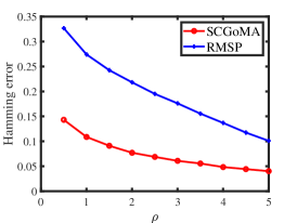
(a) Experiment 1(a)

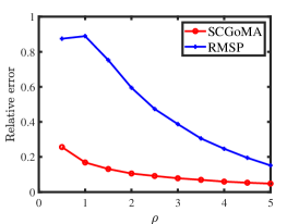
(b) Experiment 1(a)

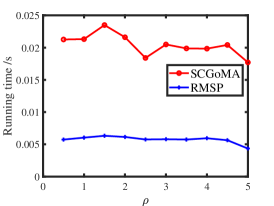
(c) Experiment 1(a)

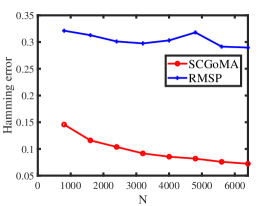
(d) Experiment 1(b)

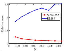
(e) Experiment 1(b)

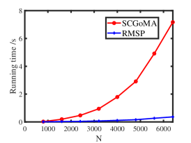
(f) Experiment 1(b)

Figure 1: Binomial distribution.

5.3.2 Uniform distribution

When $R(i,j)\sim\mathrm{Uniform}(0,2R_{0}(i,j))$ for $i\in[N],j\in[J]$:

Experiment 2(a): changing $\rho$. Let $N=800$ and $\rho$ range in $\{10,20,\ldots,100\}$.

Experiment 2(b): changing $N$. Let $\rho=1$ and $N$ range in $\{800,1600,2400,\ldots,6400\}$.

The results are displayed in Figure 2. We see that SCGoMA’s error rates are insensitive to the scaling parameter $\rho$, which verifies our findings in Instance 4. SCGoMA’s performance improves as $N$ increases, supporting our analysis following Theorem 2. Meanwhile, SCGoMA outperforms RMSP in accuracy, although RMSP is faster.

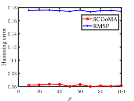
(a) Experiment 2(a)

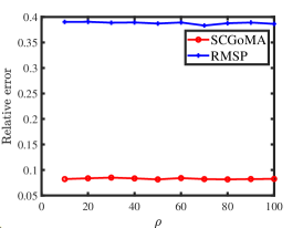
(b) Experiment 2(a)

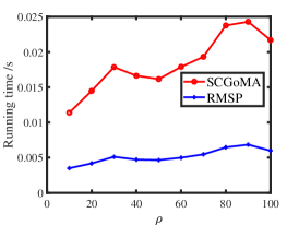
(c) Experiment 2(a)

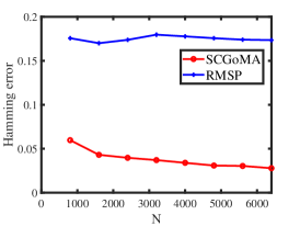
(d) Experiment 2(b)

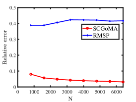
(e) Experiment 2(b)

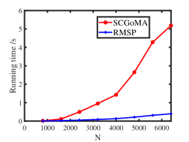
(f) Experiment 2(b)

Figure 2: Uniform distribution.

5.3.3 Normal distribution

When $R(i,j)\sim\mathrm{Normal}(R_{0}(i,j),\sigma^{2})$ for $i\in[N],j\in[J]$:

Experiment 3(a): changing $\rho$. Let $N=800,\sigma^{2}=1,$ and $\rho$ range in $\{0.5,1,1.5,\ldots,5\}$.

Experiment 3(b): changing $N$. Let $\rho=0.5,\sigma^{2}=1$, and $N$ range in $\{800,1600,,2400,\ldots,6400\}$.

Figure 3 presents the numerical results. We see that SCGoMA exhibits better performances as $\rho$ and $N$ increase, which supports our discussions in Instance 6 and Theorem 2. Although RMSP requires less time than SCGoMA, its accuracy is lower.

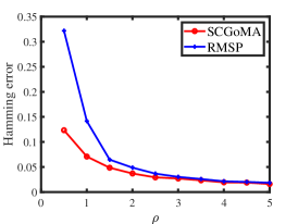
(a) Experiment 3(a)

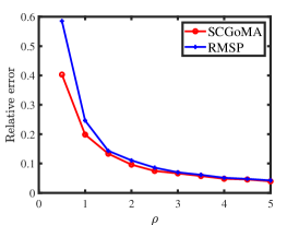
(b) Experiment 3(a)

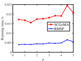
(c) Experiment 3(a)

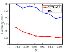
(d) Experiment 3(b)

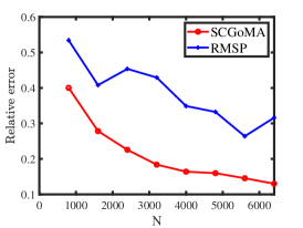
(e) Experiment 3(b)

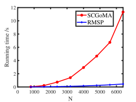
(f) Experiment 3(b)

Figure 3: Normal distribution.

5.3.4 Signed responses

When $\mathbb{P}(R(i,j)=1)=\frac{1+R_{0}(i,j)}{2}$ and $\mathbb{P}(R(i,j)=-1)=\frac{1-R_{0}(i,j)}{2}$ for $i\in[N],j\in[J]$:

Experiment 4(a): changing $\rho$. Let $N=800$ and $\rho$ range in $\{0.8,0.825,0.85,\ldots,1\}$.

Experiment 4(b): changing $N$. Let $\rho=0.2$ and $N$ range in $\{800,1600,2400,\ldots,6400\}$.

Figure 4 shows the results. We see that increasing $\rho$ and $N$ enhances the accuracy of SCGoMA, verifying our analysis in Instance 7 and Theorem 2. Despite the additional computational time required by SCGoMA compared to RMSP, SCGoMA returns more accurate estimation parameters.

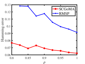
(a) Experiment 4(a)

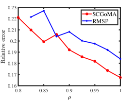
(b) Experiment 4(a)

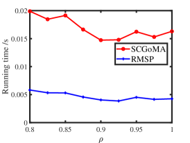
(c) Experiment 4(a)

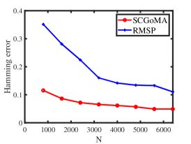
(d) Experiment 4(b)

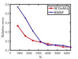
(e) Experiment 4(b)

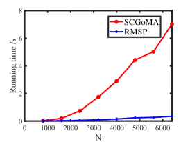
(f) Experiment 4(b)

Figure 4: Signed responses.

6 The Taylor Manifest Anxiety Scale (TMAS) data

The results presented in Section 5 have demonstrated that SCGoMA performs significantly better than RMSP in terms of accuracy. In this section, we exclusively examine the performance of our SCGoMA approach by applying it to the Taylor Manifest Anxiety Scale (TMAS) data [56]. The number of latent classes K is usually unknown for real datasets. Here, we determine K by selecting the one that minimizes the spectral norm of $R-\hat{\Pi}\hat{\Theta}^{\prime}$, i.e., $K=\mathrm{argmin}_{k\in[\mathrm{rank}(R)]}\|R-\hat{\Pi}\hat{\Theta}^{\prime}\|$, where $\hat{\Pi}$ represents the estimated membership matrix, $\hat{\Theta}$ signifies the estimated item parameter matrix, and both $\hat{\Pi}$ and $\hat{\Theta}$ are attained via Algorithm 2 with inputs $R$ and $k$.

Background. We apply SCGoMA to the TMAS data, which can be download at https://openpsychometrics.org/_rawdata/. The TMAS data contains 50 true-false statements (see panel (b) of Figure 5 for details). It also includes the gender and the age of each subject. For this dataset, 1 indicates true, 2 indicates false, and 0 means not answered. The original data has 5410 subjects. For simplicity, we do not consider age and gender in this paper. After removing those subjects that did not respond to any items, there are 5401 subjects remaining, i.e., $N=5401,J=50$, and $R\in\{0,1,2\}^{5401\times 50}$.

Analysis. The estimated number of latent classes for the TMAS data is 2. Applying the SCGoMA method to the observed weighted response matrix $R$ with $K=2$ obtains the $5401\times 2$ estimated membership matrix $\hat{\Pi}$ and the $50\times 2$ estimated item parameter matrix $\hat{\Theta}$. It takes around 0.012 seconds for SCGoMA to process this dataset.

Results. For convenience, we use class 1 and class 2 to represent the two estimated latent classes. To better understand $\hat{\Pi}$ and $\hat{\Theta}$, we plot the membership vectors of the top 50 subjects in panel (a) of Figure 5 and display the heatmap of $\hat{\Theta}$ in panel (b) of Figure 5, where we only present a subset of the subjects because the number of subjects $N=5401$ is large. Based on Equation (4), we have the following observation: for subject $i\in[N]$, given its membership score $\Pi(i,k)$ on the $k$-th latent class, if $\Theta(j,k)$ is larger, then the expected value of $R(i,j)$ is larger for the $j$-th item, i.e., $R(i,j)$ tends to be larger if $\Theta(j,k)$ is larger. Recall that in the response matrix $R$ for the TMAS data, 1 represents true and 2 represents false. The above observation suggests that for subject $i\in[N]$, item $j\in[J]$, and class $k\in[K]$, the response for the $i$-th subject to the $j$-th item tends to be false for a larger $\hat{\Theta}(j,k)$ and tends to be true for a smaller $\hat{\Theta}(j,k)$.

Based on the above analysis and carefully examining panel (b) of Figure 5, class 1 can be interpreted as individuals with a positive mindset towards life, while class 2 can be interpreted as individuals with a negative mindset towards life. Panel (b) of Figure 5 suggests that individuals belonging to class 1 tend to possess positive characteristics such as energy, gentleness, relaxation, concentration, strength, etc., while individuals belonging to class 2 tend to have an opposite mindset compared to those in class 1. Although the mindsets of class 1 and class 2 are opposite, for any individual $i\in[N]$, it has different weights towards the two classes, i.e., the $i$-th individual has different extent for negative and positive mindset towards life. For example, from the left panel of Figure (5), we find that the membership score of subject 2 is $(0.6968,0.3032)$ which can be interpreted as subject 2 having a 69.86% probability of possessing a positive mindset towards life and a 30.32% probability of possessing a negative mindset towards life. Subject 7 is an individual who holds a negative mindset towards life as his/her membership score is $(0.0377,0.9623)$. In fact, the responses of subject 7 to all items (recorded in the $7$-th row of $R$) are $R(7,:)=(2,1,2,2,1,2,1,1,1,1,1,2,2,1,2,1,1,2,2,2,1,1,1,1,1,1,1,1,2,1,1,2,2,1,1,1,1,2,2,1,1,1,1,1,1,1,1,1,1,2)$,
which are consistent with our analysis after checking the statement of each item in panel (b) of Figure 5. For subject 21, he/she is positive because his/her membership score is $(0.9047,0.0953)$. In fact, the responses of subject 21 to all items are $R(21,:)=(1,2,1,1,2,2,2,2,2,2,2,1,2,2,1,2,2,1,2,1,2,1,2,2,2,2,2,2,1,2,2,1,1,2,2,2,1,1,1,2,2,2,2,1,2,\\ 2,2,2,2,1)$, which also support our analysis. Meanwhile, it is easy to see that there are 44 opposite responses between subjects 7 and 21, and this supports our finding that subjects 7 and 21 have almost completely different mindsets towards life.

By analyzing panel (a) of Figure 5, we find that the majority of individuals in the top 50 subjects have a more negative mindset towards life than positive mindset. Actually, this finding also holds for all the 5401 individuals because $\sum_{i=1}^{5401}\hat{\Pi}(i,1)=1656.9$ and $\sum_{i=1}^{5401}\hat{\Pi}(i,2)=3744.1$. Furthermore, we say that an individual has a highly positive mindset towards life if $\hat{\Pi}(i,1)\geq 0.9$ and a highly negative mindset towards life if $\hat{\Pi}(i,2)\geq 0.9$. We are also interested in the number of individuals that have a highly positive (or negative) mindset towards life. For the TMAS data, we find that there are 51 subjects that have a highly positive mindset towards life and 910 subjects that have a highly negative mindset towards life, i.e., the number of individuals with a highly negative mindset towards life is much larger than that of individuals with a highly positive mindset towards life. The reason behind this phenomenon is profound and meaningful for social science and psychological science and it is of independent interest.

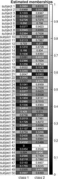
(a) Heatmap of $\hat{\Pi}$

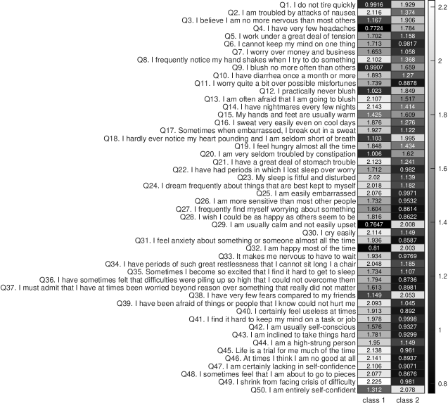
(b) Heatmap of $\hat{\Theta}$

Figure 5: Numerical results for the TMAS data.

7 Conclusion

This paper presents the Weighted Grade of Membership (WGoM) model, a novel statistical model in grade of membership analysis for categorical data with weighted responses. The proposed model allows each subject to belong to multiple latent classes and provides a generative framework for weighted response matrices based on arbitrary distribution. The Grade of Membership model, a well-known paradigm in the literature, is a special case of our WGoM framework. To the best of our knowledge, our WGoM is the first model that enables weighted responses in grade of membership analysis for categorical data. An efficient Singular Value Decomposition (SVD)-based algorithm is developed for estimating the mixed membership matrix and the item parameter matrix under the WGoM framework. We establish the rate of convergence of our method by considering the scaling parameter. It is shown that the proposed method enjoys consistent estimation under WGoM. We provide several instances to demonstrate the generality of our model and analyze the behaviors of our method when the observed weighted response matrices are generated from different distributions under WGoM. Extensive experiments are conducted to verify our theoretical findings and evaluate the effectiveness of our method.

The contribution of this paper lies in threefold: (1) the development of a novel WGoM model that overcomes the limitations of the Grade of Membership model and provides a more flexible framework for analyzing categorical data with weighted responses, thereby opening new opportunities for practical applications in various research areas. (2) the presentation of an efficient SVD-based algorithm for estimating the parameters in WGoM; and (3) the extensive evaluation of our method through theoretical analysis, simulation studies, and real-world applications, which demonstrates its effectiveness both theoretically and empirically.

Future work may explore an extension of WGoM to handle a more complex scenario that includes additional covariates. Additionally, developing a method which can effectively determine the number of latent classes under WGoM is an interesting future direction. Finally, developing more efficient algorithms to enhance the computational efficiency of the proposed method would be valuable contributions.

Declaration of Competing Interest

The author declares no competing interests.

Data availability

Data and code will be made available on request.

Appendix A Proofs under WGoM

A.1 Proof of Theorem 1

Proof.

First, we consider the case when $Q=2$. For this case, we let $\mathbb{P}(R(i,j)=a_{1})=p_{1},\mathbb{P}(R(i,j)=a_{2})=p_{2}$. $p_{1}$ and $p_{2}$ are two probabilities which should satisfy the following conditions:

$$p_{1}+p_{2}=1,0\leq p_{1}\leq 1,0\leq p_{2}\leq 1.$$ (6)

To make Equation (5) hold (i.e., $\mathbb{E}(R(i,j))=R_{0}(i,j)$), we need

$$a_{1}p_{1}+a_{2}p_{2}=R_{0}(i,j).$$ (7)

Combining Equation (6) and Equation (7) gives

$$p_{1}=\frac{a_{2}-R_{0}(i,j)}{a_{2}-a_{1}},p_{2}=\frac{R_{0}(i,j)-a_{1}}{a_{2}-a_{1}},$$

where $R_{0}(i,j)\in[a_{1},a_{2}]$. Thus, for the case $Q=2$, there exists only one discrete distribution $\mathcal{F}$ satisfying Equation (5), and the exact form of $\mathcal{F}$ is

$$\mathbb{P}(R(i,j)=a_{1})=\frac{a_{2}-R_{0}(i,j)}{a_{2}-a_{1}},\mathbb{P}(R(i,j)=a_{2})=\frac{R_{0}(i,j)-a_{1}}{a_{2}-a_{1}},$$

where $R_{0}(i,j)\in[a_{1},a_{2}]$.

Next, we consider the case when $Q\geq 3$. For this case, we let $\mathbb{P}(R(i,j)=a_{q})=p_{q}$ for $q\in[Q]$, where $p_{q}$ is a probability. Since the summation of all probabilities should be 1, $\{p_{q}\}^{Q}_{q=1}$ should satisfy

$$\sum_{q=1}^{Q}p_{q}=1,0\leq p_{q}\leq 1\mathrm{~{}for~{}}q\in[Q].$$ (8)

To make Equation (5) hold, $\{p_{q}\}^{Q}_{q=1}$ should satisfy

$$\sum_{q=1}^{Q}a_{q}p_{q}=R_{0}(i,j).$$ (9)

By analyzing Equation (8) and Equation (9), we find that the $Q$ unknown elements $\{p_{q}\}^{Q}_{q=1}$ should satisfy 2 equalities and $Q$ inequalities. Therefore, there must exist $\{p_{q}\}^{Q}_{q=1}$ satisfying Equation (8) and Equation (9).

Now, we construct $Q$ solutions of $\{p_{q}\}^{Q}_{q=1}$ that satisfy Equation (8) and Equation (9). Let $p_{2}=p_{3}=\ldots=p_{Q}\equiv y$. Equation (8) gives

$$p_{1}+(Q-1)y=1,0\leq p_{1}\leq 1,0\leq y\leq 1.$$ (10)

Equation (9) gives

$$a_{1}p_{1}+(a_{2}+a_{3}+\ldots+a_{Q})y=R_{0}(i,j).$$ (11)

Combining Equation (10) and Equation (11) gives

$$p_{1}=\frac{a_{2}+a_{3}+\ldots+a_{Q}-(Q-1)R_{0}(i,j)}{\sum_{q=1}^{Q}a_{q}-Qa_{1}},p_{2}=p_{3}=\ldots=p_{Q}=y=\frac{R_{0}(i,j)-a_{1}}{\sum_{q=1}^{Q}a_{q}-Qa_{1}},$$

where $a_{1}\leq R_{0}(i,j)\leq\frac{a_{2}+a_{3}+\ldots+a_{Q}}{Q-1}$.

Therefore, the exact form of a $\mathcal{F}$ satisfying Equation (5) is

$$\mathbb{P}(R(i,j)=a_{1})=\frac{a_{2}+a_{3}+\ldots+a_{Q}-(Q-1)R_{0}(i,j)}{\sum_{q=1}^{Q}a_{q}-Qa_{1}},\mathbb{P}(R(i,j)=a_{q})=\frac{R_{0}(i,j)-a_{1}}{\sum_{q=1}^{Q}a_{q}-Qa_{1}}\mathrm{~{}for~{}}q=2,3,\ldots,Q,$$

where $R_{0}(i,j)\in[a_{1},\frac{a_{2}+a_{3}+\ldots+a_{Q}}{Q-1}]$. Since $a_{1}<a_{2}<\ldots<a_{Q}$, we have $a_{1}<\frac{\sum_{q=2}^{Q}a_{q}}{Q-1}$, which implies that $[a_{1},\frac{a_{2}+a_{3}+\ldots+a_{Q}}{Q-1}]$, the range of $R_{0}(i,j)$, is not empty. Sure, there are $Q$ choices such that $p_{q}$ is fixed while $p_{1}=p_{2}=\ldots=p_{q-1}=p_{q+1}=\ldots=p_{Q}$ for $q\in[Q]$. Therefore, there are at least $Q$ distinct discrete distributions $\mathcal{F}$ satisfying Equation (5). ∎

A.2 Proof of Proposition 1

Proof.

Point (a) of Theorem 2 in [42] always holds provided that each latent class has at least one pure subject and $\Theta$ is a rank-$K$ matrix, thus it guarantees WGoM’s identifiability since WGoM requires $\Pi$ to satisfy Equation (3) and $\Theta$’s rank to be $K$. Note that as stated by point (b) of Theorem 2 in [42], WGoM is also identifiable if $\Theta$’s rank is $(K-1)$ and $\Theta$ satisfies some extra conditions in point (b) of Theorem 2 in [42]. However, we only consider the case $\mathrm{rank}(\Theta)=K$ in this paper mainly for the convenience of our further theoretical analysis. ∎

A.3 Proof of Lemma 1

Proof.

Since $R_{0}=\Pi\Theta^{\prime}=U\Sigma V^{\prime}$, we have $U=R_{0}V\Sigma^{-1}=\Pi\Theta^{\prime}V\Sigma^{-1}=\Pi X$, where we set $X$ as $\Theta^{\prime}V\Sigma^{-1}$. Since $U=\Pi X$ and we have assumed that $\Pi(\mathcal{I},:)=I_{K\times K}$, we have $U(\mathcal{I},:)=\Pi(\mathcal{I},:)X=X$, i.e., $X=U(\mathcal{I},:)$. ∎

A.4 Basic properties of $R_{0}$

The following lemmas are useful for building our main theoretical result.

Lemma 2.

Under $WGoM(\Pi,\Theta,\mathcal{F})$, for $i\in[N],j\in[J]$, we have

$$\sqrt{\frac{1}{K\lambda_{1}(\Pi^{\prime}\Pi)}}\leq\|U(i,:)\|_{F}\leq\sqrt{\frac{1}{\lambda_{K}(\Pi^{\prime}\Pi)}}\mathrm{~{}and~{}}0\leq\|V(j,:)\|_{F}\leq\frac{K^{1.5}\kappa(\Pi)}{\sqrt{\lambda_{K}(B^{\prime}B)}}.$$

Proof.

For $U$, since $U=\Pi X$ by Lemma 1, we have

$$\mathrm{min}_{i\in[N]}\|e^{\prime}_{i}U\|^{2}_{F}=\mathrm{min}_{i\in[N]}e^{\prime}_{i}UU^{\prime}e_{i}=\mathrm{min}_{i\in[N]}\Pi(i,:)XX^{\prime}\Pi^{\prime}(i,:)=\mathrm{min}_{i\in[N]}\|\Pi(i,:)\|^{2}_{F}\frac{\Pi(i,:)}{\|\Pi(i,:)\|_{F}}XX^{\prime}\frac{\Pi^{\prime}(i,:)}{\|\Pi(i,:)\|_{F}}$$

$$\geq\mathrm{min}_{i\in[N]}\|\Pi(i,:)\|^{2}_{F}\mathrm{min}_{\|y\|_{F}=1}y^{\prime}XX^{\prime}y=\mathrm{min}_{i\in[N]}\|\Pi(i,:)\|^{2}_{F}\lambda_{K}(XX^{\prime})\overset{\mathrm{By~{}Lemma~{}}\ref{P3}}{=}\frac{\mathrm{min}_{i\in[N]}\|\Pi(i,:)\|^{2}_{F}}{\lambda_{1}(\Pi^{\prime}\Pi)}\geq\frac{1}{K\lambda_{1}(\Pi^{\prime}\Pi)},$$

where the last inequality holds since $\|\Pi(i,:)\|_{F}\geq\|\Pi(i,:)\|_{1}/\sqrt{K}=1/\sqrt{K}$ for $i\in[N]$ and $e_{i}$ is a $N\times 1$ vector with $i$-th entry being 1 while the other entries being zero. Meanwhile,

$$\mathrm{max}_{i\in[N]}\|e^{\prime}_{i}U\|^{2}_{F} =\mathrm{max}_{i\in[N]}\|\Pi(i,:)\|^{2}_{F}\frac{\Pi(i,:)}{\|\Pi(i,:)\|_{F}}XX^{\prime}\frac{\Pi^{\prime}(i,:)}{\|\Pi(i,:)\|_{F}}\leq\mathrm{max}_{i\in[N]}\|\Pi(i,:)\|^{2}_{F}\mathrm{max}_{\|y\|_{F}=1}y^{\prime}XX^{\prime}y$$

$$=\mathrm{max}_{i\in[N]}\|\Pi(i,:)\|^{2}_{F}\lambda_{1}(XX^{\prime})\overset{\mathrm{By~{}Lemma~{}}\ref{P3}}{=}\frac{\mathrm{max}_{i\in[N]}\|\Pi(i,:)\|^{2}_{F}}{\lambda_{K}(\Pi^{\prime}\Pi)}\leq\frac{1}{\lambda_{K}(\Pi^{\prime}\Pi)}.$$

For $V$, recall that $R_{0}=\Pi\Theta^{\prime}=U\Sigma V^{\prime},\Theta=\rho B,\mathrm{max}_{j\in[J],k\in[K]}|B(j,k)|=1$, and $U^{\prime}U=I_{K\times K}$, we have $V=\Theta\Pi^{\prime}U\Sigma^{-1}$ which gives that

$$\mathrm{max}_{j\in[J]}\|V(j,:)\|_{F} =\mathrm{max}_{j\in[J]}\rho\|B(i,:)\Pi^{\prime}U\Sigma^{-1}\|_{F}\leq\mathrm{max}_{j\in[J]}\rho\|B(i,:)\Pi^{\prime}U\|_{F}\|\Sigma^{-1}\|_{F}=\mathrm{max}_{j\in[J]}\rho\|B(i,:)\Pi^{\prime}\|_{F}\|\Sigma^{-1}\|_{F}$$

$$\leq\mathrm{max}_{j\in[J]}\rho\|B(i,:)\Pi^{\prime}\|_{F}\frac{\sqrt{K}}{\sigma_{K}(R_{0})}\overset{\mathrm{By~{}Lemma~{}}\ref{P4}}{\leq}\mathrm{max}_{j\in[J]}\|B(i,:)\Pi^{\prime}\|_{F}\frac{\sqrt{K}}{\sigma_{K}(\Pi)\sigma_{K}(B)}$$

$$\leq\mathrm{max}_{j\in[J]}\|B(i,:)\|_{F}\|\Pi\|_{F}\frac{\sqrt{K}}{\sigma_{K}(\Pi)\sigma_{K}(B)}\leq\frac{K\|\Pi\|_{F}}{\sigma_{K}(\Pi)\sigma_{K}(B)}\leq\frac{K^{1.5}\|\Pi\|}{\sigma_{K}(\Pi)\sigma_{K}(B)}=\frac{K^{1.5}\kappa(\Pi)}{\sigma_{K}(B)},$$

where we have used the fact that $\|Y\|_{F}\leq\sqrt{\mathrm{rank}(Y)}\|Y\|$ for any matrix $Y$. The lower bound of $\|V(j,:)\|_{F}$ is 0 because $\|B(i,:)\|_{F}$ can be set as 0. ∎

Lemma 3.

Under $WGoM(\Pi,\Theta,\mathcal{F})$, we have

$$\lambda_{1}(XX^{\prime})=\frac{1}{\lambda_{K}(\Pi^{\prime}\Pi)}\mathrm{~{}and~{}}\lambda_{K}(XX^{\prime})=\frac{1}{\lambda_{1}(\Pi^{\prime}\Pi)}.$$

Proof.

Recall that $U=\Pi X$ by Lemma 1 and $U^{\prime}U=I_{K\times K}$, we have $I_{K\times K}=X^{\prime}\Pi^{\prime}\Pi X$. Because $X$ is a nonsingular matrix, we have $\Pi^{\prime}\Pi=(XX^{\prime})^{-1}$, which gives

$$\lambda_{1}(XX^{\prime})=\frac{1}{\lambda_{K}(\Pi^{\prime}\Pi)},\lambda_{K}(XX^{\prime})=\frac{1}{\lambda_{1}(\Pi^{\prime}\Pi)}.$$

∎

Lemma 4.

Under $WGoM(\Pi,\Theta,\mathcal{F})$, we have

$$\sigma_{K}(R_{0})\geq\rho\sigma_{K}(\Pi)\sigma_{K}(B)\mathrm{~{}and~{}}\sigma_{1}(R_{0})\leq\rho\sigma_{1}(\Pi)\sigma_{1}(B).$$

Proof.

For $\sigma_{K}(R_{0})$, we have

$$\sigma^{2}_{K}(R_{0})=\lambda_{K}(R_{0}R^{\prime}_{0}) =\lambda_{K}(\Pi\Theta^{\prime}\Theta\Pi^{\prime})=\lambda_{K}(\Pi^{\prime}\Pi\Theta^{\prime}\Theta)\geq\lambda_{K}(\Pi^{\prime}\Pi)\lambda_{K}(\Theta^{\prime}\Theta)=\lambda_{K}(\Pi^{\prime}\Pi)\lambda_{K}(\rho^{2}B^{\prime}B)=\rho^{2}\sigma^{2}_{K}(\Pi)\sigma^{2}_{K}(B),$$

where we have frequently used the fact the nonzero eigenvalues of $Y_{1}Y_{2}$ are equal to that of $Y_{2}Y_{1}$ for any two matrices $Y_{1}$ and $Y_{2}$.

For $\sigma_{1}(R_{0})$, we have

$$\sigma_{1}(R_{0})=\|R_{0}\|=\rho\|\Pi B^{\prime}\|\leq\rho\|\Pi\|\|B\|=\rho\sigma_{1}(\Pi)\sigma_{1}(B).$$

∎

A.5 Proof of Theorem 2

Proof.

Similar to Theorem 3.1 [52], we obtain the row-wise eigenspace error first. Define $H_{\hat{U}}$ as $H_{\hat{U}}=\hat{U}^{\prime}U$. Let $H_{\hat{U}}=U_{H_{\hat{U}}}\Sigma_{H_{\hat{U}}}V^{\prime}_{H_{\hat{U}}}$ be the top $K$ SVD of $H_{\hat{U}}$. Set $\mathrm{sgn}(H_{\hat{U}})=U_{H_{\hat{U}}}V^{\prime}_{H_{\hat{U}}}$. Define $H_{\hat{V}}$ as $H_{\hat{V}}=\hat{V}^{\prime}V$, let $H_{\hat{V}}=U_{H_{\hat{V}}}\Sigma_{H_{\hat{V}}}V^{\prime}_{H_{\hat{V}}}$ be the top K SVD of $H_{\hat{V}}$, and set $\mathrm{sgn}(H_{\hat{V}})=U_{H_{\hat{V}}}V^{\prime}_{H_{\hat{V}}}$. For $i\in[N],j\in[J]$, the following statements are true:

• $\mathbb{E}(R(i,j)-R_{0}(i,j))=0$ under WGoM.

• $\mathbb{E}((R(i,j)-R_{0}(i,j))^{2})=\mathrm{Var}(R(i,j))\leq\rho\gamma$.

• Set $\mu=\mathrm{max}(\frac{N\|U\|^{2}_{2\rightarrow\infty}}{K},\frac{J\|V\|^{2}_{2\rightarrow\infty}}{K})$ as the incoherence parameter introduced in Definition 3.1. of [57]. Based on Lemma 2 and Condition 1, we have $\frac{N\|U\|^{2}_{2\rightarrow\infty}}{K}\leq\frac{N}{K\lambda_{K}(\Pi^{\prime}\Pi)}=O(1)$ and $\frac{J\|V\|^{2}_{2\rightarrow\infty}}{K}\leq\frac{JK^{3}\kappa^{2}(\Pi)}{K\lambda_{K}(B^{\prime}B)}=O(1)$. Therefore, we have $\mu=O(1)$.

• Let $c_{b}=\frac{\tau}{\sqrt{\rho\gamma\mathrm{max}(N,J)/(\mu\mathrm{log}(N+J))}}$. By $\mu=O(1)$ and Assumption 1, we have $c_{b}\leq O(1)$.

• By Lemma 4 and Condition 1, we have $\kappa(R_{0})=\frac{\sigma_{1}(R_{0})}{\sigma_{K}(R_{0})}\leq\kappa(\Pi)\kappa(B)=O(1)$.

By the first four statements, we see that all conditions of Theorem 4.4 [57] are satisfied. Then, according to Theorem 4.4. [57], when $\sigma_{K}(R_{0})\gg\sqrt{\rho\gamma(N+J)\mathrm{log}(N+J)}$, with probability at least $1-O(\frac{1}{(N+J)^{5}})$, we have

$$\mathrm{max}(\|\hat{U}\mathrm{sgn}(H_{\hat{U}})-U\|_{2\rightarrow\infty},\|\hat{V}\mathrm{sgn}(H_{\hat{V}})-V\|_{2\rightarrow\infty}) \leq C\frac{\sqrt{\rho\gamma K\mathrm{log}(N+J)})+\sqrt{\rho\gamma K}\kappa(R_{0})\sqrt{\frac{\mathrm{max}(N,J)}{\mathrm{min}(N,J)}\mu}}{\sigma_{K}(R_{0})}$$

$$=O(\frac{\sqrt{\rho\gamma K\mathrm{log}(N+J)}}{\sigma_{K}(R_{0})})\leq O(\frac{\sqrt{\rho\gamma K\mathrm{log}(N+J)}}{\rho\sigma_{K}(\Pi)\sigma_{K}(B)}),$$

where the last inequality holds by Lemma 4. Set $\varpi=\mathrm{max}(\|\hat{U}\hat{U}^{\prime}-UU^{\prime}\|_{2\rightarrow\infty},\|\hat{V}\hat{V}^{\prime}-VV^{\prime}\|_{2\rightarrow\infty})$ as the row-wise eigenspace error. Because $\|\hat{U}\hat{U}^{\prime}-UU^{\prime}\|_{2\rightarrow\infty}\leq 2\|U-\hat{U}\mathrm{sgn}(H_{\hat{U}})\|_{2\rightarrow\infty}$ and $\|\hat{V}\hat{V}^{\prime}-VV^{\prime}\|_{2\rightarrow\infty}\leq 2\|V-\hat{V}\mathrm{sgn}(H_{\hat{V}})\|_{2\rightarrow\infty}$, we have

$$\varpi=O(\frac{\sqrt{\rho\gamma K\mathrm{log}(N+J)}}{\rho\sigma_{K}(\Pi)\sigma_{K}(B)}).$$ (12)

The per-subject error rates of the membership matrix $\Pi$ are the same as that of mixed membership community detection. By the proofs of Theorem 3.2 [52] and Theorem 1 [58], we know that with probability at least $1-O(\frac{1}{(N+J)^{5}})$, there exists a $K\times K$ permutation matrix $\mathcal{P}$ such that for $i\in[N]$,

$$\|e^{\prime}_{i}(\hat{\Pi}-\Pi\mathcal{P})\|_{1}=O(\varpi\kappa(\Pi^{\prime}\Pi)K\sqrt{\lambda_{1}(\Pi^{\prime}\Pi)}).$$ (13)

By Equations (12)-(13) and Condition 1, we have

$$\|e^{\prime}_{i}(\hat{\Pi}-\Pi\mathcal{P})\|_{1}=O(\varpi\kappa(\Pi^{\prime}\Pi)K\sqrt{\lambda_{1}(\Pi^{\prime}\Pi)})=O(\sqrt{\frac{\gamma\mathrm{log}(N+J)}{\rho J}}).$$ (14)

If we do not consider Condition 1, though we can always obtain the bound of $\|e^{\prime}_{i}(\hat{\Pi}-\Pi\mathcal{P})\|_{1}$ using Equation (13), we can not get the transparent form provided in Equation (14) since we fail to simplify $\varpi$ without Condition 1 when we use Theorem 4.4 of [57] to obtain $\varpi$’s upper bound.

Next, we consider the theoretical upper bound of $\|\hat{\Theta}-\Theta\mathcal{P}\|$. First, we have

$$\|\hat{\Theta}-\Theta\mathcal{P}\| =\|\hat{R}^{\prime}\hat{\Pi}(\hat{\Pi}^{\prime}\hat{\Pi})^{-1}-R^{\prime}_{0}\Pi(\Pi^{\prime}\Pi)^{-1}\mathcal{P}\|$$

$$=\|(\hat{R}^{\prime}-R^{\prime}_{0})\hat{\Pi}(\hat{\Pi}^{\prime}\hat{\Pi})^{-1}+R^{\prime}_{0}(\hat{\Pi}(\hat{\Pi}^{\prime}\hat{\Pi})^{-1}-\Pi(\Pi^{\prime}\Pi)^{-1}\mathcal{P})\|\leq\|(\hat{R}^{\prime}-R^{\prime}_{0})\hat{\Pi}(\hat{\Pi}^{\prime}\hat{\Pi})^{-1}\|+\|R^{\prime}_{0}(\hat{\Pi}(\hat{\Pi}^{\prime}\hat{\Pi})^{-1}-\Pi(\Pi^{\prime}\Pi)^{-1}\mathcal{P})\|$$

$$\leq\|\hat{R}-R_{0}\|\|\hat{\Pi}(\hat{\Pi}^{\prime}\hat{\Pi})^{-1}\|+\|R_{0}\|\hat{\Pi}(\hat{\Pi}^{\prime}\hat{\Pi})^{-1}-\Pi(\Pi^{\prime}\Pi)^{-1}\mathcal{P}\|\leq 2\|R-R_{0}\|\|\hat{\Pi}(\hat{\Pi}^{\prime}\hat{\Pi})^{-1}\|+\|R_{0}\|\hat{\Pi}(\hat{\Pi}^{\prime}\hat{\Pi})^{-1}-\Pi(\Pi^{\prime}\Pi)^{-1}\mathcal{P}\|$$

$$=2\|R-R_{0}\|\|\hat{\Pi}(\hat{\Pi}^{\prime}\hat{\Pi})^{-1}\|+\|\rho\Pi B^{\prime}\|\hat{\Pi}(\hat{\Pi}^{\prime}\hat{\Pi})^{-1}-\Pi(\Pi^{\prime}\Pi)^{-1}\mathcal{P}\|$$

$$\leq 2\|R-R_{0}\|\|\hat{\Pi}(\hat{\Pi}^{\prime}\hat{\Pi})^{-1}\|+\rho\|\Pi\|\|B\|\|\hat{\Pi}(\hat{\Pi}^{\prime}\hat{\Pi})^{-1}-\Pi(\Pi^{\prime}\Pi)^{-1}\mathcal{P}\|$$

$$=\frac{2\|R-R_{0}\|}{\sigma_{K}(\hat{\Pi})}+\rho\sigma_{1}(\Pi)\sigma_{1}(B)\|\hat{\Pi}(\hat{\Pi}^{\prime}\hat{\Pi})^{-1}-\Pi(\Pi^{\prime}\Pi)^{-1}\mathcal{P}\|.$$ (15)

The upper bound of $\|\hat{\Theta}-\Theta\mathcal{P}\|$ can be obtained immediately as long as we can obtain the lower bound of $\sigma_{K}(\hat{\Pi})$, the upper bounds of $\|R-R_{0}\|$ and $\|\hat{\Pi}(\hat{\Pi}^{\prime}\hat{\Pi})^{-1}-\Pi(\Pi^{\prime}\Pi)^{-1}\mathcal{P}\|$. We bound the three terms subsequently.

For $\sigma_{K}(\hat{\Pi})$, Weyl’s inequality for singular values [59] gives us:

$$|\sigma_{K}(\hat{\Pi})-\sigma_{K}(\Pi)|\leq\|\hat{\Pi}-\Pi\mathcal{P}\|\leq\sqrt{N}\mathrm{~{}max}_{i\in[N]}\|e^{\prime}_{i}(\hat{\Pi}-\Pi\mathcal{P})\|_{1}\overset{\mathrm{By~{}Equation~{}}\ref{boundPihat}}{=}O(\sqrt{\frac{\gamma N\mathrm{log}(N+J)}{\rho J}}).$$ (16)

Then we have $\sigma_{K}(\hat{\Pi})\geq\sigma_{K}(\Pi)-O(\sqrt{\frac{\gamma N\mathrm{log}(N+J)}{\rho J}})$. Note that $\sigma_{K}(\Pi)=O(\sqrt{\frac{N}{K}})$ by Condition 1 and $\frac{\gamma\mathrm{log}(N+J)}{\rho J}\ll 1$ should hold to make the error rate in Equation (14) close to zero, we have $\sigma_{K}(\Pi)-O(\sqrt{N}\sqrt{\frac{\gamma\mathrm{log}(N+J)}{\rho J}})=O(\sqrt{N/K})$, i.e.,

$$\sigma_{K}(\hat{\Pi})\geq O(\sqrt{N/K}).$$ (17)

For the term $\|R-R_{0}\|$, when Assumption 1 holds, Lemma 2 of [60] says that, with probability at least $1-o((N+J)^{-5})$, we have

$$\|R-R_{0}\|=O(\sqrt{\gamma\rho\mathrm{max}(N,J)\mathrm{log}(N+J)}).$$ (18)

For $\|\hat{\Pi}(\hat{\Pi}^{\prime}\hat{\Pi})^{-1}-\Pi(\Pi^{\prime}\Pi)^{-1}\mathcal{P}\|$, by Condition 1, Equation (16), and Equation (17), we have

$$\|\hat{\Pi}(\hat{\Pi}^{\prime}\hat{\Pi})^{-1}-\Pi(\Pi^{\prime}\Pi)^{-1}\mathcal{P}\| =\|(\hat{\Pi}-\Pi\mathcal{P})(\hat{\Pi}^{\prime}\hat{\Pi})^{-1}+\Pi(\mathcal{P}(\hat{\Pi}^{\prime}\hat{\Pi})^{-1}-(\Pi^{\prime}\Pi)^{-1}\mathcal{P})\|$$

$$\leq\|\hat{\Pi}-\Pi\mathcal{P}\|\|(\hat{\Pi}^{\prime}\hat{\Pi})^{-1}\|+\|\Pi\|\|\mathcal{P}(\hat{\Pi}^{\prime}\hat{\Pi})^{-1}-(\Pi^{\prime}\Pi)^{-1}\mathcal{P}\|$$

$$=\frac{\|\hat{\Pi}-\Pi\mathcal{P}\|}{\sigma^{2}_{K}(\hat{\Pi})}+\sigma_{1}(\Pi)\|\mathcal{P}(\hat{\Pi}^{\prime}\hat{\Pi})^{-1}-(\Pi^{\prime}\Pi)^{-1}\mathcal{P}\|$$

$$\leq\frac{\|\hat{\Pi}-\Pi\mathcal{P}\|_{F}}{\sigma^{2}_{K}(\hat{\Pi})}+\sigma_{1}(\Pi)\|\mathcal{P}(\hat{\Pi}^{\prime}\hat{\Pi})^{-1}-(\Pi^{\prime}\Pi)^{-1}\mathcal{P}\|$$

$$\leq\frac{\|\hat{\Pi}-\Pi\mathcal{P}\|_{F}}{\sigma^{2}_{K}(\hat{\Pi})}+\sigma_{1}(\Pi)(\|(\hat{\Pi}^{\prime}\hat{\Pi})^{-1}\|+\|(\Pi^{\prime}\Pi)^{-1}\|)$$

$$=\frac{\|\hat{\Pi}-\Pi\mathcal{P}\|_{F}}{\sigma^{2}_{K}(\hat{\Pi})}+\sigma_{1}(\Pi)(\frac{1}{\sigma^{2}_{K}(\hat{\Pi})}+\frac{1}{\sigma^{2}_{K}(\Pi)})$$

$$=O(\sqrt{\frac{\gamma\mathrm{log}(N+J)}{\rho NJ}})+O(\sqrt{\frac{1}{N}})=O(\sqrt{\frac{1}{N}}).$$ (19)

By Condition 1, Equations (15), (17), (18), and (19), we have

$$\|\hat{\Theta}-\Theta\mathcal{P}\| =O(\sqrt{\frac{\gamma\rho\mathrm{max}(N,J)\mathrm{log}(N+J)}{N}})+O(\rho\sqrt{J}).$$

Since $\|\hat{\Theta}-\Theta\mathcal{P}\|_{F}\leq\sqrt{K}\|\hat{\Theta}-\Theta\mathcal{P}\|$, by Condition 1, we have

$$\|\hat{\Theta}-\Theta\mathcal{P}\|_{F}=O(\sqrt{\frac{\gamma\rho\mathrm{max}(N,J)\mathrm{log}(N+J)}{N}})+O(\rho\sqrt{J}).$$

Since $\|\Theta\|_{F}\geq\|\Theta\|=\rho\sigma_{1}(B)=O(\rho\sqrt{\frac{J}{K}})=O(\rho\sqrt{J})$ by Condition 1, we have

$$\frac{\|\hat{\Theta}-\Theta\mathcal{P}\|_{F}}{\|\Theta\|_{F}}=O(\sqrt{\frac{\gamma\mathrm{max}(N,J)\mathrm{log}(N+J)}{\rho NJ}}).$$

Remark 4.

By Lemma 4 and Condition 1, we have $\sigma_{K}(R_{0})\geq O(\rho\sqrt{NJ})$. Since $\rho\sqrt{NJ}\gg\sqrt{\rho\gamma(N+J)\mathrm{log}(N+J)}=O(\sqrt{\rho\gamma N\mathrm{log}(N+J)})$ by Condition 1 $\Leftrightarrow\rho J\gg\gamma\mathrm{log}(N+J)$, we see that the inequality $\sigma_{K}(R_{0})\gg\sqrt{\rho\gamma(N+J)\mathrm{log}(N+J)}$ (this inequality is required when we use Theorem 4.4. [57]) holds naturally as long as the bound in Equation (14) is sufficiently small, i.e., $\rho J\gg\gamma\mathrm{log}(N+J)$.

∎

Appendix B Extra instances

Here, we provide another two instances when $R$’s elements take 3 (or 2) distinct values.

Instance 8.

Suppose that the elements of $R$ range in $\{-2,1,1.5\}$ (although real-world responses may not take values like $\{-2,1,1.5\}$, we still consider this case to emphasize the generality of our WGoM). We aim at constructing a discrete distribution $\mathcal{F}$ satisfying Equation (5), where $R\in\{-2,1,1.5\}^{N\times J}$ can be generated from distribution $\mathcal{F}$ under our WGoM. Next, we discuss how to construct $\mathcal{F}$. Let $\mathbb{P}(R(i,j)=-2)=p_{1},\mathbb{P}(R(i,j)=1)=p_{2},$ and $\mathbb{P}(R(i,j)=1.5)=p_{3}$, where $p_{q}\geq 0$ for $q\in[3]$. Because the summation of all probabilities should be 1, we have

$$p_{1}+p_{2}+p_{3}=1.$$ (20)

To make Equation (5) hold, we need

$$\mathbb{E}(R(i,j))=-2p_{1}+p_{2}+1.5p_{3}\equiv R_{0}(i,j).$$ (21)

Combine Equation (20) with Equation (21), by simple calculation, we have

$$p_{2}=3-7p_{1}-2R_{0}(i,j),p_{3}=6p_{1}+2R_{0}(i,j)-2.$$ (22)

For simplicity, assume that $p_{1}=R_{0}(i,j)$. Then Equation (22) gives

$$p_{1}=R_{0}(i,j),p_{2}=3-9R_{0}(i,j),p_{3}=8R_{0}(i,j)-2.$$ (23)

Because $p_{1}\in[0,1],p_{2}\in[0,1],p_{3}\in[0,1]$, $R_{0}(i,j)$ should satisfy $R_{0}(i,j)\in[\frac{1}{4},\frac{1}{3}]$. As a result, the discrete distribution $\mathcal{F}$ should be specified as

$$\mathbb{P}(R(i,j)=-2)=R_{0}(i,j),\mathbb{P}(R(i,j)=1)=3-9R_{0}(i,j),\mathbb{P}(R(i,j)=1.5)=8R_{0}(i,j)-2,$$ (24)

where $R_{0}(i,j)$’s range is $[\frac{1}{4},\frac{1}{3}]$. When $\mathcal{F}$ is set as Equation (24), we can generate a $R\in\{-2,1,1.5\}^{N\times J}$ from our model WGoM. Equation (24) also gives that $\mathrm{Var}(R_{0}(i,j))=-R^{2}_{0}(i,j)+13R_{0}(i,j)-\frac{3}{2}$. Note that for this case, since $R_{0}(i,j)\in[\frac{1}{4},\frac{1}{3}]$ and $R_{0}=\Pi\Theta^{\prime}$, we have $\Theta(j,k)\in[\frac{1}{4},\frac{1}{3}]$ for $j\in[J],k\in[K]$. Therefore, it’s meaningless to set $\Theta=\rho B$ where $\mathrm{max}_{j\in[J],k\in[K]}|B(j,k)|=1$. Instead, we should use $\Theta$ to replace $\rho B$ in the proof of Theorem 2, which gives that Assumption 1 is a lower bound requirement of $N$ (and $J$) and there is no need to consider $\rho$ and $\gamma$ anymore. Furthermore, we set $p_{1},p_{2},p_{3}$ in Equation (23) as a solution of Equations (20) and (21), actually, there exist other solutions satisfying Equations (20) and (21) by Theorem 1. For example, we can also set $\mathcal{F}$ as

$$\mathbb{P}(R(i,j)=-2)=-R_{0}(i,j),\mathbb{P}(R(i,j)=1)=3+5R_{0}(i,j),\mathbb{P}(R(i,j)=1.5)=-4R_{0}(i,j)-2,$$

where $R_{0}(i,j)\in[-\frac{3}{5},-\frac{1}{2}]$. Therefore, there are many possible solutions to make Equations (20) and (21) hold.

Instance 9.

Suppose that $R$’s entries range in $\{-2,1\}$. By Theorem 1, $\mathcal{F}$ should be defined as

$$\mathbb{P}(R(i,j)=-2)=\frac{1-R_{0}(i,j)}{3},\mathbb{P}(R(i,j)=1)=\frac{2+R_{0}(i,j)}{3},$$

where $R_{0}(i,j)\in[-2,1]$. We also have $\mathrm{Var}(R(i,j))=-R^{2}_{0}(i,j)-R_{0}(i,j)+2$, which ranges in $[0,\frac{9}{4}]$. Since $R_{0}=\Pi\Theta^{\prime}$, we see that $\Theta(j,k)\in[-2,1]$ for $j\in[J],k\in[K]$. Because $\Theta\in[-2,1]^{J\times K}$, if we set $\Theta=\rho B$ such that $\mathrm{max}_{j\in[J],k\in[K]}|B(j,k)|=1$, we see that $\rho$’s range is $(0,2]$ when all entries of $B$ are negative and $\rho$’s range is $(0,1]$ when $B$’s entries are non-negative. We also have $\tau\leq 4$ and $\gamma=\frac{9}{4\rho}$. Setting $\gamma=\frac{9}{4\rho}$ in Theorem 2, we see that increasing $\rho$ improves SCGoMA’s performance.

References

• [1] J. R. Landis, G. G. Koch, The measurement of observer agreement for categorical data, biometrics (1977) 159–174.
• [2] K.-Y. Liang, S. L. Zeger, B. Qaqish, Multivariate regression analyses for categorical data, Journal of the Royal Statistical Society: Series B (Methodological) 54 (1) (1992) 3–24.
• [3] D. K. Pokholok, C. T. Harbison, S. Levine, M. Cole, N. M. Hannett, T. I. Lee, G. W. Bell, K. Walker, P. A. Rolfe, E. Herbolsheimer, et al., Genome-wide map of nucleosome acetylation and methylation in yeast, Cell 122 (4) (2005) 517–527.
• [4] T. F. Jaeger, Categorical data analysis: Away from ANOVAs (transformation or not) and towards logit mixed models, Journal of memory and language 59 (4) (2008) 434–446.
• [5] A. Agresti, Categorical data analysis, Vol. 792, John Wiley & Sons, 2012.
• [6] J. Oser, M. Hooghe, S. Marien, Is online participation distinct from offline participation? a latent class analysis of participation types and their stratification, Political research quarterly 66 (1) (2013) 91–101.
• [7] D. Huang, R. Li, H. Wang, Feature screening for ultrahigh dimensional categorical data with applications, Journal of Business & Economic Statistics 32 (2) (2014) 237–244.
• [8] G. Wang, C. Zou, G. Yin, Change-point detection in multinomial data with a large number of categories, The Annals of Statistics 46 (5) (2018) 2020 – 2044.
• [9] O. Ovaskainen, N. Abrego, P. Halme, D. Dunson, Using latent variable models to identify large networks of species-to-species associations at different spatial scales, Methods in Ecology and Evolution 7 (5) (2016) 549–555.
• [10] C. Skinner, Analysis of categorical data for complex surveys, International Statistical Review 87 (2019) S64–S78.
• [11] A. Brown, U. Böckenholt, Intermittent faking of personality profiles in high-stakes assessments: A grade of membership analysis., Psychological methods.
• [12] E. D. Klonsky, T. M. Olino, Identifying clinically distinct subgroups of self-injurers among young adults: a latent class analysis., Journal of consulting and clinical psychology 76 (1) (2008) 22.
• [13] S. T. Lanza, B. L. Rhoades, Latent class analysis: an alternative perspective on subgroup analysis in prevention and treatment, Prevention science 14 (2) (2013) 157–168.
• [14] K. Nylund-Gibson, A. Y. Choi, Ten frequently asked questions about latent class analysis., Translational Issues in Psychological Science 4 (4) (2018) 440.
• [15] C. M. Ulbricht, S. A. Chrysanthopoulou, L. Levin, K. L. Lapane, The use of latent class analysis for identifying subtypes of depression: A systematic review, Psychiatry Research 266 (2018) 228–246.
• [16] B. E. Weller, N. K. Bowen, S. J. Faubert, Latent class analysis: a guide to best practice, Journal of Black Psychology 46 (4) (2020) 287–311.
• [17] P. Sinha, C. S. Calfee, K. L. Delucchi, Practitioner’s guide to latent class analysis: methodological considerations and common pitfalls., Critical care medicine 49 (1) (2021) e63.
• [18] L. A. Goodman, Exploratory latent structure analysis using both identifiable and unidentifiable models, Biometrika 61 (2) (1974) 215–231.
• [19] E. S. Garrett, S. L. Zeger, Latent class model diagnosis, Biometrics 56 (4) (2000) 1055–1067.
• [20] T. Asparouhov, B. Muthén, Using Bayesian priors for more flexible latent class analysis, in: proceedings of the 2011 joint statistical meeting, Miami Beach, FL, American Statistical Association Alexandria, VA, 2011.
• [21] A. White, T. B. Murphy, BayesLCA: An R package for Bayesian latent class analysis, Journal of Statistical Software 61 (2014) 1–28.
• [22] Y. Li, J. Lord-Bessen, M. Shiyko, R. Loeb, Bayesian latent class analysis tutorial, Multivariate behavioral research 53 (3) (2018) 430–451.
• [23] P. G. Van der Heijden, J. Dessens, U. Bockenholt, Estimating the concomitant-variable latent-class model with the EM algorithm, Journal of Educational and Behavioral Statistics 21 (3) (1996) 215–229.
• [24] Z. Bakk, J. K. Vermunt, Robustness of stepwise latent class modeling with continuous distal outcomes, Structural equation modeling: a multidisciplinary journal 23 (1) (2016) 20–31.
• [25] H. Chen, L. Han, A. Lim, Beyond the EM algorithm: constrained optimization methods for latent class model, Communications in Statistics-Simulation and Computation 51 (9) (2022) 5222–5244.
• [26] Y. Gu, G. Xu, A joint MLE Approach to Large-Scale Structured Latent Attribute Analysis, Journal of the American Statistical Association 118 (541) (2023) 746–760.
• [27] A. Anandkumar, R. Ge, D. Hsu, S. M. Kakade, M. Telgarsky, Tensor decompositions for learning latent variable models, Journal of machine learning research 15 (2014) 2773–2832.
• [28] Z. Zeng, Y. Gu, G. Xu, A Tensor-EM Method for Large-Scale Latent Class Analysis with Binary Responses, Psychometrika 88 (2) (2023) 580–612.
• [29] J. Jin, Z. T. Ke, S. Luo, Mixed membership estimation for social networks, Journal of Econometrics.
• [30] M. A. Woodbury, J. Clive, A. Garson Jr, Mathematical typology: a grade of membership technique for obtaining disease definition, Computers and biomedical research 11 (3) (1978) 277–298.
• [31] D. M. Blei, A. Y. Ng, M. I. Jordan, Latent dirichlet allocation, Journal of machine Learning research 3 (Jan) (2003) 993–1022.
• [32] H. Al-Asadi, K. K. Dey, J. Novembre, M. Stephens, Inference and visualization of DNA damage patterns using a grade of membership model, Bioinformatics 35 (8) (2019) 1292–1298.
• [33] K. K. Dey, C. J. Hsiao, M. Stephens, Visualizing the structure of RNA-seq expression data using grade of membership models, PLoS genetics 13 (3) (2017) e1006599.
• [34] Q. Li, H. Sun, D. E. Boufford, B. Bartholomew, P. W. Fritsch, J. Chen, T. Deng, R. H. Ree, Grade of Membership models reveal geographical and environmental correlates of floristic structure in a temperate biodiversity hotspot, New Phytologist 232 (3) (2021) 1424–1435.
• [35] Z. T. Ke, M. Wang, Using SVD for topic modeling, Journal of the American Statistical Association (2022) 1–16.
• [36] A. Jainarayanan, N. Mouroug-Anand, E. H. Arbe-Barnes, A. J. Bush, R. Bashford-Rogers, A. Frampton, L. Heij, M. Middleton, M. L. Dustin, E. Abu-Shah, et al., Pseudotime dynamics of T cells in pancreatic ductal adenocarcinoma inform distinct functional states within the regulatory and cytotoxic t cells, Iscience 26 (4).
• [37] E. A. Erosheva, S. E. Fienberg, C. Joutard, Describing disability through individual-level mixture models for multivariate binary data, The annals of applied statistics 1 (2) (2007) 346.
• [38] I. C. Gormley, T. B. Murphy, A grade of membership model for rank data, Bayesian Analysis 4 (2009) 265–295.
• [39] Y. Gu, E. A. Erosheva, G. Xu, D. B. Dunson, Dimension-grouped mixed membership models for multivariate categorical data, Journal of Machine Learning Research 24 (88) (2023) 1–49.
• [40] H. D. Tolley, K. G. Manton, Large sample properties of estimates of a discrete grade of membership model, Annals of the Institute of Statistical Mathematics 44 (1992) 85–95.
• [41] M. J. Beal, Variational algorithms for approximate Bayesian inference, University of London, University College London (United Kingdom), 2003.
• [42] L. Chen, Y. Gu, A Spectral Method for Identifiable Grade of Membership Analysis with Binary Responses, arXiv preprint arXiv:2305.03149.
• [43] E. A. Erosheva, Comparing latent structures of the grade of membership, Rasch, and latent class models, Psychometrika 70 (4) (2005) 619–628.
• [44] M. E. Newman, Analysis of weighted networks, Physical review E 70 (5) (2004) 056131.
• [45] J. Leskovec, D. Huttenlocher, J. Kleinberg, Governance in social media: A case study of the wikipedia promotion process, in: Proceedings of the International AAAI Conference on Web and Social Media, Vol. 4, 2010, pp. 98–105.
• [46] P. Massa, M. Salvetti, D. Tomasoni, Bowling alone and trust decline in social network sites, in: 2009 Eighth IEEE International Conference on Dependable, Autonomic and Secure Computing, IEEE, 2009, pp. 658–663.
• [47] K. Goldberg, T. Roeder, D. Gupta, C. Perkins, Eigentaste: A constant time collaborative filtering algorithm, information retrieval 4 (2001) 133–151.
• [48] S. Kumar, F. Spezzano, V. Subrahmanian, C. Faloutsos, Edge weight prediction in weighted signed networks, in: 2016 IEEE 16th International Conference on Data Mining (ICDM), IEEE, 2016, pp. 221–230.
• [49] G. G. Van de Bunt, M. A. Van Duijn, T. A. Snijders, Friendship networks through time: An actor-oriented dynamic statistical network model, Computational & Mathematical Organization Theory 5 (1999) 167–192.
• [50] G. Guo, J. Zhang, N. Yorke-Smith, A novel evidence-based bayesian similarity measure for recommender systems, ACM Transactions on the Web (TWEB) 10 (2) (2016) 1–30.
• [51] J. Kunegis, Konect: the koblenz network collection, in: Proceedings of the 22nd international conference on world wide web, 2013, pp. 1343–1350.
• [52] X. Mao, P. Sarkar, D. Chakrabarti, Estimating mixed memberships with sharp eigenvector deviations, Journal of the American Statistical Association 116 (536) (2021) 1928–1940.
• [53] M. C. U. Araújo, T. C. B. Saldanha, R. K. H. Galvao, T. Yoneyama, H. C. Chame, V. Visani, The successive projections algorithm for variable selection in spectroscopic multicomponent analysis, Chemometrics and intelligent laboratory systems 57 (2) (2001) 65–73.
• [54] N. Gillis, S. A. Vavasis, Semidefinite programming based preconditioning for more robust near-separable nonnegative matrix factorization, SIAM Journal on Optimization 25 (1) (2015) 677–698.
• [55] J. Lei, A. Rinaldo, Consistency of spectral clustering in stochastic block models, Annals of Statistics 43 (1) (2015) 215–237.
• [56] J. A. Taylor, Taylor manifest anxiety scale, Journal of Consulting Psychology.
• [57] Y. Chen, Y. Chi, J. Fan, C. Ma, et al., Spectral methods for data science: A statistical perspective, Foundations and Trends® in Machine Learning 14 (5) (2021) 566–806.
• [58] H. Qing, J. Wang, Bipartite Mixed Membership Distribution-Free Model. A novel model for community detection in overlapping bipartite weighted networks, Expert Systems with Applications (2023) 121088.
• [59] H. Weyl, Das asymptotische Verteilungsgesetz der Eigenwerte linearer partieller Differentialgleichungen (mit einer Anwendung auf die Theorie der Hohlraumstrahlung), Mathematische Annalen 71 (4) (1912) 441–479.
• [60] H. Qing, J. Wang, Community detection for weighted bipartite networks, Knowledge-Based Systems 274 (2023) 110643.