Restricted Tweedie Stochastic Block Models

Abstract

The stochastic block model (SBM) is a widely used framework for community detection in networks, where the network structure is typically represented by an adjacency matrix. However, conventional SBMs are not directly applicable to an adjacency matrix that consists of non-negative zero-inflated continuous edge weights. To model the international trading network, where edge weights represent trading values between countries, we propose an innovative SBM based on a restricted Tweedie distribution. Additionally, we incorporate nodal information, such as the geographical distance between countries, and account for its dynamic effect on edge weights. Notably, we show that given a sufficiently large number of nodes, estimating this covariate effect becomes independent of community labels of each node when computing the maximum likelihood estimator of parameters in our model. This result enables the development of an efficient two-step algorithm that separates the estimation of covariate effects from other parameters. We demonstrate the effectiveness of our proposed method through extensive simulation studies and an application to real-world international trading data.

Keywords: Stochastic block model, community detection, network analysis, compound Poisson-Gamma distributions, dynamic effects.

1 Introduction

1.1 Background

A community can be conceptualized as a collection of nodes that exhibit similar connection patterns in a network. Community detection is a fundamental problem in network analysis, with wide applications in social network (Bedi and Sharma, 2016), marketing (Bakhthemmat and Izadi, 2021), recommendation systems (Gasparetti et al., 2021), and political polarization detection (Guerrero-Solé, 2017). Identifying communities in a network not only enables nodes to be clustered according to their connections with each other, but also reveals the hierarchical structure that many real-world networks exhibit. Furthermore, it can facilitate network data processing, analysis, and storage (Lu et al., 2018).

Among the various methods for detecting communities in a network, the Stochastic Block Model (SBM) stands out as a probabilistic graph model. It is founded based on the stochastic equivalence assumption, positing that the connecting probability between node $i$ and node $j$ depends solely on their community memberships (Holland et al., 1983). If we assume that given the community memberships of two nodes $i$ and $j$, denoted by $c_{i}$ and $c_{j}$, the edge weight between them is Bernoulli distributed. In particular, letting $Y_{ij}$ denote this weight, the adjacency matrix $Y=(Y_{ij})$ is generated as

$$Y_{ij}\mid c_{i}=k,c_{j}=l\sim\text{Bernoulli}(B_{kl}),$$ (1)

where $B_{kl}$ denotes the probability of connectivity between the nodes from the $k$th and $l$th communities.

As indicated in (1), an SBM provides an interpretable representation of the network’s community structure. Moreover, an SBM can be efficiently fitted with various algorithms, such as maximum likelihood estimation and Bayesian inference (Lee and Wilkinson, 2019). In recent few years, there has been extensive research on theoretical properties of the estimators obtained from these algorithms (Lee and Wilkinson, 2019).

In this paper, we are motivated to leverage the remarkable capability of the SBM in detecting latent community structures to tackle an interesting problem—clustering countries into different groups based on their international trading patterns. However, in this application, we encounter three fundamental challenges that can not be addressed by existing SBM models.

1.2 Three main challenges

1.2.1 Edge Weights

The classical SBM, as originally proposed by Holland et al. (1983), is primarily designed for binary networks, as indicated in (1). However, in the context of the international trading network, we are presented with richer data, encompassing not only the presence or absence of trading relations between countries but also the specific trading volumes in dollars. These trading volumes serve as the intensity and strength of the trading relationships between countries. In such cases, thresholding the data to form a binary network would inevitably result in a loss of valuable information.

In the literature, several methods have been developed to extend the modelling of edge weights beyond the binary range. Some methods leverages distributions capable of handling edge weights. For instance, Aicher et al. (2013, 2015) adopt a Bayesian approach to model edge weights using distributions from the exponential family. Ludkin (2020) allows for arbitrary distributions in modeling edge weights and sample the posterior distribution using a reversible jump Markov Chain Monte Carlo (MCMC) method. Ng and Murphy (2021) and Motalebi et al. (2021) use a compound Bernoulli-Gamma distribution and a Hurdle model to represent edge weights respectively. Haj et al. (2022) apply the binomial distribution to networks with integer-valued edge weights that are bounded from above. In contrast, there is a growing interest in multilayer networks, where edge weights are aggregated across network layers. Notable examples of research in this area include the work by MacDonald et al. (2022) and Chen and Mo (2022).

However, the above approaches cannot properly deal with financial data that involve non-negative continuous random variables with a large number of zeros and a right-skewed distribution.

1.2.2 Incorporating nodal information

Many SBMs assume that nodes within the same community exhibit stochastic equivalence. However, this assumption can be restrictive and unrealistic, as real-world networks are influenced by environmental factors, individual node characteristics, and edge properties, leading to heterogeneity among community members that affects network formation. Depending on the relationship between communities and covariates, there are generally three classes of models, as shown in Figure 1. Models (b) and (c) have been previously discussed by Huang et al. (2023). We are also particularly interested in model (c), where latent community labels and covariates jointly shape the network structure. In our study on international trading networks, factors such as the geographical distance between countries, along with community labels, play critical roles in shaping trading relations. Neglecting these influential factors can significantly compromise the accuracy of SBM estimations.

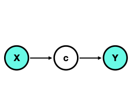
(a) Covariates-driven

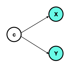
(b) Covariates-confounding

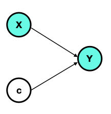
(c) Covariates-adjusted

Figure 1: Three network models with covariates. The symbols $X$, $Y$ and $c$ represent covariates, network connection and community memberships, respectively. A shaded/unshaded cell means the corresponding quantity is observable/latent.

Various works in the past have considered the incorporation of nodal information. For instance, Roy et al. (2019) and Choi et al. (2012) considered a pairwise covariate effect in the logistic link function when modelling the edge between two nodes. In contrast, Ma et al. (2020) and Hoff et al. (2002) incorporated the pairwise covariate effect but with a latent space model. Other research considering covariates in an SBM includes Tallberg (2004), Vu et al. (2013) and Peixoto (2018). Moreover, Mariadassou et al. (2010) and Huang et al. (2023) addressed the dual challenge of incorporating the covariates and modeling the edge weights by assuming that each integer-valued edge weight follows a Poisson distribution and accounting for the pairwise covariates into the mean.

While the aforementioned literature has made significant progress in incorporating covariate information into network modeling, the complexity escalates when we confront the third challenge — the observed network is changing over time. This challenge necessitates a deeper exploration of how covariates influence network formation dynamically — a facet that remains unaddressed in the existing literature.

1.2.3 Dynamic network

Recent advances in capturing temporal network data demand the extension of classic SBMs to dynamic settings, as previous research predominantly focused on static networks.

Researchers have attempted to adapt SBMs to dynamic settings, employing various strategies such as state-space models, hidden Markov chains, and change point detection. Fu et al. (2009) and Xing et al. (2010) extended a mixed membership SBM for static networks to dynamic networks by characterizing the evolving community memberships and block connection probabilities with a state space model. Both Yang et al. (2011) and Xu and Hero (2014) studied a sequence of SBMs, where the parameters were dynamically linked by a hidden Markov chain. Matias and Miele (2017) applied Markov chains to the evolution of the node community labels over time. Bhattacharjee et al. (2020) proposed a method to detect a single change point such that the community connection probabilities are different constants within the two intervals separated by it. Xin et al. (2017) characterized the occurrence of a connection between any two nodes in an SBM using an inhomogeneous Poisson process. Zhang et al. (2020) proposed a regularization method for estimating the network parameters at adjacent time points to achieve smoothness.

1.3 Our contributions

The main contribution of this paper is to extend the classical SBM to address the three challenges mentioned above. Given the community membership of each node, we generalize the assumption that edges in the network follow Bernoulli distributions to that they follow compound Poisson-Gamma distributions instead (Section 2). This allows us to model edges that can take on any non-negative real value, including exactly zero itself. Later in Section 6, we apply the proposed model to an international trading network, where each edge between two countries represents the dollar amount of their trading values, for which our model is more appropriate than the classical one. Moreover, not only do we incorporate nodal information in the form of covariates, we also allow the effects of these covariates to be time-varying (Section 2).

We use a variational approach (Section 4) to conduct statistical inference for such a time-varying network. We also prove an interesting result (Section 3) that, asymptotically, the covariate effects in our model can be estimated irrespective of how community labels are assigned to each node. This result also allows us to use an efficient two-step algorithm (Section 4), separating the estimation of the covariate effects and that of the other parameters—including the unknown community labels. A similar two-step procedure is also used by Huang et al. (2023).

2 Methodology

In this section, we first give a brief review of a rarely-used distribution, the Tweedie distribution, which can be used to model network edges with zero or positive continuous weights. Next, we propose a general SBM using the Tweedie distribution in three successive steps, each addressing a challenge mentioned in Section 1.2. More specifically, we start with a vanilla model, a variation of the classic SBM where each edge value between two nodes now follows the Tweedie distribution rather than the Bernoulli distribution. We then incorporate covariate terms into the model, before we finally arrive at a time-varying version of the model by allowing the covariates to have dynamic effects that change over time.

2.1 Tweedie distribution

Let $N$ be a random variable following the Poisson distribution with mean $\lambda$. Conditional on $N=n$, $Z_{1},\ldots,Z_{n}\overset{iid}{\sim}\text{Gamma}(\alpha,\gamma)$. Define

$$Y=\left\{\begin{aligned} 0,\quad\quad\quad\quad\quad\quad\quad\,\,\,\,&\quad\rm{if}\quad N=0,\\ Z_{1}+Z_{2}+\cdots+Z_{N},&\quad\rm{if}\quad N=1,2,3,\cdots.\end{aligned}\right.$$

Then, $Y$ has a compound Poisson-gamma distribution, with a nonzero probability mass at $0$. As $Y=0$ if and only if $N=0$, $\mathbb{P}(Y=0)=\mathbb{P}(N=0)=\exp{(-\lambda)}$. Conditional on $N=n>0$, $Y$ follows a gamma distribution with mean $n\alpha\gamma$ and variance $n\alpha\gamma^{2}$. In the context of international trading (also see Section 6 below), $N$ may be the number of trades in a given year; $Z_{1},\dots,Z_{N}$ may be the dollar amount of each trade; then, $Y$ is the simply total trading amount from that year.

The compound Poisson-gamma distribution, known as a special case of the Tweedie distribution (Tweedie, 1984), is related to an exponential dispersion (ED) family. If $Y$ follows an ED family distribution with mean $\mu$ and variance function $V$, then $Y$ satisfies $\textnormal{var}(Y)=\phi V(\mu)$ for some dispersion parameter $\phi$. The Tweedie distribution belongs to the ED family with $V(\mu)=\mu^{\rho}$ for some constant $\rho$. Specified by different values of $\rho$, the Tweedie distribution includes the normal ($\rho=0$), the gamma ($\rho=2$) and the inverse Gaussian distribution ($\rho=3$), and the scaled Poisson distribution ($\rho=1$). Tweedie distributions exist for all values of $\rho$ outside the interval $(0,1)$. Of special interest to us here is the restricted Tweedie distribution with $1<\rho<2$, which is the aforementioned compound Poisson–gamma distribution with a positive mass at zero but a continuous distribution of positive values elsewhere. We add the word “restricted” to describe the Tweedie distribution when $\rho$ is constrained to lie on the interval $(1,2)$; it will become clearer later in Section 4 that this particular restriction also simplifies the overall estimation procedure somewhat.

Specifically, the aforementioned compound Poisson–gamma distribution with parameters $(\lambda,\alpha,\gamma)$ can be reparameterized as a restricted Tweedie distribution, with parameters $(\mu,\phi,\rho)$ satisfying $1<\rho<2$ and the following relationships:

$$\lambda=\dfrac{\mu^{2-\rho}}{\phi(2-\rho)},\quad\alpha=\dfrac{2-\rho}{\rho-1},\quad\gamma=\phi(\rho-1)\mu^{\rho-1}.$$

That is, the marginal distribution of $Y$, defined above, can be expressed as

$$f(y|\mu,\phi,\rho)=a(y,\phi,\rho)\cdot\exp\left\{\frac{1}{\phi}\left(\dfrac{y\mu^{1-\rho}}{1-\rho}-\dfrac{\mu^{2-\rho}}{2-\rho}\right)\right\},\quad 1<\rho<2,$$ (2)

where

$$a(y,\phi,\rho)=\left\{\begin{aligned} \dfrac{1}{y}\sum\limits_{j=1}^{\infty}\dfrac{y^{j\alpha}}{(\rho-1)^{j\alpha}\phi^{j(1+\alpha)}(2-\rho)^{j}j!\Gamma(j\alpha)},&\quad\rm{for}\quad y>0,\\ 1,\quad\quad\quad\quad\quad\quad\quad\quad\quad\quad\quad\quad\quad\quad\quad\,\,&\quad\rm{for}\quad y=0.\end{aligned}\right.$$

2.2 Vanilla model

Let $\mathcal{G}=(V,E)$ denote a weighted graph, where $V$ denotes a set of nodes with cardinality $|V|=n$ and $E$ denotes the set of edges between two nodes. For SBMs, each node in the network can belong to one of $K$ groups. Let $c_{i}\in\{1,\cdots,K\}$ denote the unobserved community membership of node $i$ and $c_{i}$ follows a multinomial distribution with the probability $\pi=(\pi_{1},\cdots,\pi_{K})$.

Usually, the set $E$ is represented by an $n\times n$ matrix $Y=[y_{ij}]\in\mathbb{R}^{n\times n}$. In classical SBMs, each $y_{ij}$ is modelled either as a Bernoulli random variable taking on binary values of 0 or 1, or as a Poisson random variable taking on non-negative integer values. We first relax this restriction by allowing $y_{ij}$ to take on non-negative real values. Since we focus on an undirected weighted network without self-loops, $Y$ is a (for us, non-negative) real-valued symmetric matrix with zero diagonal entries.

Given the observed data set $D=\{y_{ij}\}_{1\leq i<j\leq n}$, we assume that each edge value $y_{ij}$ follows a restricted Tweedie distribution with power $\rho\in(1,2)$ and dispersion $\phi$:

$$y_{ij}\sim\text{Tw}(\mu_{ij},\phi,\rho),\quad{\color[rgb]{0,0,0}1<\rho<2},$$ (3)

where the mean $\mu_{ij}$ is modelled as a positive constant determined by the latent community label of nodes $i$ and $j$ through a log-link function, i.e.,

$$\log(\mu_{ij})=\beta_{0}^{kl},\quad\text{if}\quad c_{i}=k\quad\text{and}\quad c_{j}=l,$$ (4)

where $\beta_{0}=[\beta_{0}^{kl}]\in\mathbb{R}^{K\times K}$ is a symmetric matrix. For a constant model, the log-link may not appear to be necessary, but it will become more useful later on as we incorporate covariates into this baseline model.

2.3 Model with covariates

In many real-life situations, we observe additional information about the network. For example, in addition to the relative existence or importance of each edge, a collection of $p$ symmetric covariate matrices ${\color[rgb]{0,0,0}X^{(1)},...,X^{(p)}}\in\mathbb{R}^{n\times n}$ may also be available, where the $(i,j)$-th entry $x_{ij}^{(u)}$ of each $X^{(u)}$ represents a pair-wise covariate containing some information about the connection between node $i$ and node $j$, and $x_{ii}^{(u)}=0$ for all $1\leq i\leq n$ and $u=1,...,p$. Given a data set $D=\{Y,{\color[rgb]{0,0,0}X^{(1)},...,X^{(p)}}\}$, the vanilla model from Section 2.2 above can be easily extended by replacing (4) with

$$\log(\mu_{ij})=\beta_{0}^{kl}+\boldsymbol{x}_{ij}^{\top}\boldsymbol{\beta},\quad\text{if}\quad c_{i}=k\quad\text{and}\quad c_{j}=l,$$ (5)

so that $\mu_{ij}$ is affected not only by the community labels $c_{i},c_{j}$ but also by the covariates contained in $\boldsymbol{x}_{ij}$. Here, both $\boldsymbol{x}_{ij}\equiv(x_{ij}^{(1)},...,x_{ij}^{(p)})^{\top}$ and $\boldsymbol{\beta}$ are $p$-dimensional vectors.

2.4 Time-varying model

Now suppose we observe an evolving network at a series of $T$ discrete time points $\{t_{1},\cdots,t_{T}\}$, with a common set of $n$ nodes. Specifically, our data set is of the form $D=\{Y(t_{1}),\dots,Y(t_{T});X^{(1)},\dots,X^{(p)}\}$. Without loss of generality, we may assume each $t_{\nu}\in[0,1]$.

To model such data, we assume in this paper that the latent community labels $c_{1},\dots,c_{n}$ are fixed over time but allow the covariate effects to change over time by incorporating a varying-coefficient model. In reality, the community labels may also change over time, but a fundamentally different set of tools will be required to model these changes and we will study them separately—not in this paper. Here, we simply assume that model (3) holds pointwise at every time point $t$, i.e.,

$$y_{ij}(t)\sim\text{Tw}(\mu_{ij}(t),\phi,\rho),\quad{\color[rgb]{0,0,0}1<\rho<2},$$ (6)

and

$$\log\{\mu_{ij}(t)\}=\beta_{0}^{kl}+\boldsymbol{x}_{ij}^{\top}\boldsymbol{\beta}(t),\quad\text{if}\quad c_{i}=k\quad\text{and}\quad c_{j}=l,$$ (7)

where $\boldsymbol{\beta}(t)\equiv(\beta_{1}(t),\dots,\beta_{p}(t))^{\top}$ and each $\beta_{u}(t)$ is a smooth function of time. The full likelihood function corresponding to our time-varying model (6)–(7) is given by

$$L(\beta_{0},\boldsymbol{\beta}(t),\pi,\phi,\rho;D,c)=\prod\limits_{i=1}^{n}\prod\limits_{k=1}^{K}\pi_{k}^{\mathds{1}(c_{i}=k)}\prod\limits_{\nu=1}^{T}\prod\limits_{1\leq i<j\leq n}\prod\limits_{k,l=1}^{K}\biggl{[}a(y_{ij}(t_{\nu}),\phi,\rho)\times\\ \exp\left\{\dfrac{1}{\phi}\left(\dfrac{y_{ij}(t_{\nu})\exp[(1-\rho)\{\beta_{0}^{kl}+\boldsymbol{x}_{ij}^{\top}\boldsymbol{\beta}(t_{\nu})\}]}{1-\rho}-\right.\right.\\ \left.\left.\dfrac{\exp[(2-\rho)\{\beta_{0}^{kl}+\boldsymbol{x}_{ij}^{\top}\boldsymbol{\beta}(t_{\nu})\}]}{2-\rho}\right)\right\}\biggr{]}^{\mathds{1}(c_{i}=k,c_{j}=l)}.$$ (8)

The likelihood functions for the earlier, simpler models—namely, the vanilla model in Section 2.2 and the static model with covairates in Section 2.3—are simply special cases of (8).

3 Theory

The resulting log-likelihood based on (8) contains three additive terms: the first involves only $\pi$; the second involves only $(\phi,\rho)$; and the third is the only one that involves both $\beta_{0}$ and $\boldsymbol{\beta}(t)$. Define

$$\ell_{n}(\boldsymbol{\beta}(t),\phi_{0},\rho_{0};D,z)\equiv\frac{1}{\binom{n}{2}}\sum\limits_{\nu=1}^{T}\sum\limits_{1\leq i<j\leq n}\sum\limits_{k,l=1}^{K}\dfrac{\mathds{1}(z_{i}=k,z_{j}=l)}{\phi_{0}}\times\\ \left(\dfrac{y_{ij}(t_{\nu})\exp[(1-\rho_{0})\{\hat{\beta}_{0}^{kl}(\boldsymbol{\beta}(t_{\nu}))+\boldsymbol{x}_{ij}^{\top}\boldsymbol{\beta}(t_{\nu})\}]}{1-\rho_{0}}-\right.\\ \left.\dfrac{\exp[(2-\rho_{0})\{\hat{\beta}_{0}^{kl}(\boldsymbol{\beta}(t_{\nu}))+\boldsymbol{x}_{ij}^{\top}\boldsymbol{\beta}(t_{\nu})\}]}{2-\rho_{0}}\right)$$ (9)

to be the aforementioned third term after having

• replaced the unknown labels $c=(c_{1},\dots,c_{n})$ with an arbitrary set of labels $z=(z_{1},\dots,z_{n})$, where each $z_{i}$ is independently multinomial$(p_{1},\dots,p_{K})$;

• profiled out the parameter $\beta_{0}$ by replacing it with $\hat{\beta}_{0}(\boldsymbol{\beta}(t))$, while presuming $\phi=\phi_{0}$ and $\rho=\rho_{0}$ to be known and fixed; and

• re-scaled it by the total number of pairs, $\binom{n}{2}$.

This quantity turns out to be very interesting. Not only does $\hat{\beta}_{0}(\boldsymbol{\beta}(t))$ have an explicit expression, but (9) can also be shown to converge to a quantity not dependent on $z$ as $n$ tends to infinity.

In other words, it does not matter that $z$ is a set of arbitrarily assigned labels! This has immediate computational implications (see Section 4). Some high-level details of this theory are spelled out below in Section 3.1, while actual proofs are given in the Appendix.

3.1 Details

To simplify the notation, we first define two population parameters,

$$\theta=\sum\limits_{\nu=1}^{T}\mathbb{E}[y_{ij}(t_{\nu})\exp\{(1-\rho_{0})\boldsymbol{x}_{ij}^{\top}\boldsymbol{\beta}(t_{\nu})\}]\quad\text{and}\quad\gamma=\sum\limits_{\nu=1}^{T}\mathbb{E}[\exp\{(2-\rho_{0})\boldsymbol{x}_{ij}^{\top}\boldsymbol{\beta}(t_{\nu})\}].$$

For these to be properly defined, we require the following two conditions, which are fairly standard and not fundamentally restrictive.

Condition 3.1.

The covariates $\{\boldsymbol{x}_{ij},1\leq i<j\leq n\}$ are i.i.d., and there exists some $\alpha>0$ such that $\mathbb{P}(\exp\{\boldsymbol{x}_{ij}^{\top}\boldsymbol{u}\}\geq\delta)\leq 2\exp(-\delta^{2}/\alpha)$ for any $\delta>0$, $i\neq j$ and $\boldsymbol{u}\in\mathbb{R}^{p}$ satisfying $\|\boldsymbol{u}\|_{2}=\sqrt{u_{1}^{2}+\dots+u_{p}^{2}}=1$.

Condition 3.2.

The function $\beta_{u}(t)$ is continuous on $[0,1]$, for all $u=1,\ldots,p$.

The corresponding empirical versions of $\theta$ and $\gamma$ between any two groups, $k$ and $l$, according to an arbitrary community label assignment, $z$, are given by

$$\hat{\theta}_{kl} =\dfrac{1}{\binom{n}{2}}\sum\limits_{\nu=1}^{T}\sum\limits_{1\leq i<j\leq n}y_{ij}(t_{\nu})\exp[(1-\rho_{0})\boldsymbol{x}_{ij}^{\top}\boldsymbol{\beta}(t_{\nu})]\mathds{1}(z_{i}=k,z_{j}=l),$$

$$\hat{\gamma}_{kl} =\dfrac{1}{\binom{n}{2}}\sum\limits_{\nu=1}^{T}\sum\limits_{1\leq i<j\leq n}\exp[(2-\rho_{0})\boldsymbol{x}_{ij}^{\top}\boldsymbol{\beta}(t_{\nu})]\mathds{1}(z_{i}=k,z_{j}=l).$$

We can then establish the following main theorem.

Theorem 1.

Theorem 1. As $n\rightarrow\infty$ while $K$ remains constant,

$$\ell_{n}(\boldsymbol{\beta}(t),\phi_{0},\rho_{0};D,z)=\dfrac{1}{\phi_{0}}\dfrac{1}{(1-\rho_{0})(2-\rho_{0})}\sum\limits_{k,l=1}^{K}\hat{\theta}_{kl}^{2-\rho_{0}}\cdot\hat{\gamma}_{kl}^{\rho_{0}-1}\\ =\dfrac{1}{\phi_{0}}\dfrac{1}{(1-\rho_{0})(2-\rho_{0})}\theta^{2-\rho_{0}}\cdot\gamma^{\rho_{0}-1}+o_{p}(1).$$ (10)

Remark 1.

So far, we have simply written $\hat{\theta}_{kl}$, $\hat{\gamma}_{kl}$, $\theta$ and $\gamma$ in order to keep the notation short. To better appreciate the conclusion of the theorem, however, it is perhaps important for us to emphasize here that these quantities are more properly written as $\hat{\theta}_{kl}(\boldsymbol{\beta}(t),\rho_{0};D,z)$, $\hat{\gamma}_{kl}(\boldsymbol{\beta}(t),\rho_{0};D,z)$, $\theta(\boldsymbol{\beta}(t),\rho_{0};D)$, and $\gamma(\boldsymbol{\beta}(t),\rho_{0};D)$.

The implication here is that, asymptotically, our inference about $\boldsymbol{\beta}(t)$ is not affected by the community labels—nor is it affected by the total number of communities, $K$, since $z$ can follow any multinomial$(p_{1},\dots,p_{K})$ distribution, including those with some $p_{k}=0$. Thus, even if we got $K$ wrong, our inference about $\boldsymbol{\beta}(t)$ would still be correct.

4 Estimation Method

4.1 Two-step Estimation

In this section, we outline an algorithm to fit the restricted Tweedie SBM. Since, for us, the parameter $\rho$ is restricted to the interval $(1,2)$, we find it sufficient to simply perform a grid search (e.g., Dunn and Smyth, 2005, 2008; Lian et al., 2023) over an equally-spaced sequence, say, $1<\rho_{1}<\dots<\rho_{m}<2$, to determine its “optimal” value. However, our empirical experiences also indicate that a sufficiently accurate estimate of $\rho$ is important for making correct inferences on other quantities of interest, including the latent community labels $c$.

For any given $\rho_{0}$ in a pre-specified sequence/grid, we propose an efficient two-step algorithm to estimate the other parameters. In Step 1 (Section 4.1.1), we obtain an estimate $\hat{\boldsymbol{\beta}}_{\rho_{0}}(t)$ of $\boldsymbol{\beta}(t)$ using an arbitrary set of community labels. This is made possible by the theoretical result earlier in Section 3. In Step 2 (Section 4.1.2), we obtain estimates of the remaining parameters parameters—$\hat{\beta}_{0}(\rho_{0}),\hat{\pi}(\rho_{o}),\hat{\phi}(\rho_{0})$—while keeping $\hat{\boldsymbol{\beta}}_{\rho_{0}}(t)$ fixed. The optimal $\rho$ is then chosen to be

$$\hat{\rho}=\operatorname*{arg\,max}\limits_{\rho_{0}\in\{\rho_{1},\cdots,\rho_{m}\}}L(\hat{\beta}_{0}(\rho_{0}),\hat{\boldsymbol{\beta}}_{\rho_{0}}(t),\hat{\pi}(\rho_{0}),\hat{\phi}(\rho_{0}),\rho_{0};D,c).$$

4.1.1 Step 1: Estimation of Covariates Coefficients

It is clear from our earlier theoretical result in Section 3 that, when $\rho=\rho_{0}$ is given and fixed, the quantity (9) can be used directly as a criterion to estimate $\boldsymbol{\beta}(t)$. To begin, here one can fix the parameter $\phi$ at $\phi_{0}=1$, since it only appears as a scaling constant in (9) and does not affect the optimum. The main computational saving afforded by Theorem 1 is that we can use an arbitrary set of labels $z$ to carry out this step, estimating $\boldsymbol{\beta}(t)$ separately without simultaneously concerning ourselves with $\beta_{0}$ or having to make inference on $c$. Both of those tasks can be temporarily delayed until after $\boldsymbol{\beta}(t)$ is estimated.

For our static model (Section 2.3), we use the optim function in R to maximize (9) directly over $\boldsymbol{\beta}$, with $T=1$. For our time-varying model (Section 2.4), we add (component-wise) smoothness penalties to (9) and estimate $\boldsymbol{\beta}(t)$ as

$$\hat{\boldsymbol{\beta}}_{\rho_{0}}(t)=\operatorname*{arg\,max}_{\boldsymbol{\beta}(t)}\ \ell_{n}(\boldsymbol{\beta}(t),1,\rho_{0};D,z)-\frac{1}{2}\sum\limits_{u=1}^{p}\lambda_{u}\cdot\int\{\boldsymbol{\beta}_{u}^{\prime\prime}(t)\}^{2}dt.$$ (11)

The penalty parameters $\lambda_{1},\dots,\lambda_{p}$ are chosen by cross-validation (see Section 4.2 below). With given penalty parameters, technical details for calculating (11) are provided in the Appendix.

4.1.2 Step 2: Variational Inference

In Step 2, with the estimate $\hat{\boldsymbol{\beta}}_{\rho_{0}}(t)$ from Step 1 (and, again, a pre-fixed $\rho=\rho_{0}$), we estimate the remaining parameters $\beta_{0}$, $\pi$, and $\phi$, as well as make inferences about the latent label $c$.

If we directly optimized the likelihood function (8) using the EM algorithm, the E-step would require us to compute $\mathbb{E}_{c|D}(\cdot)$ but, here, the conditional distribution of the latent variable $c$ given $D$ is complicated because $c_{i}$ and $c_{j}$ are not conditionally independent in general. We will use a variational approach instead.

To proceed, it will be more natural for us to emphasize the fact that (8) is really just the joint distribution of $(D,c)$. Thus, instead of writing it as $L(\beta_{0},\boldsymbol{\beta}(t),\pi,\phi,\rho;D,c)$, in this section we will write it simply as $\mathbb{P}(D,c;\beta_{0},\pi,\phi)$, where we have also dropped $\boldsymbol{\beta}(t)$ and $\rho$ to keep the notation short because, within this step, $\rho=\rho_{0}$ and $\boldsymbol{\beta}(t)=\hat{\boldsymbol{\beta}}_{\rho_{0}}(t)$ are both fixed and not being estimated.

Ideally, since the latent variable $c$ is not observable, one may want to work with the marginal distribution of $D$ and estimate $(\beta_{0},\pi,\phi)$ as:

$$\left(\hat{\beta}_{0},\hat{\pi},\hat{\phi}\right) =\operatorname*{arg\,max}\limits_{\beta_{0},\pi,\phi}\log\mathbb{P}(D;\beta_{0},\pi,\phi)$$

$$=\operatorname*{arg\,max}\limits_{\beta_{0},\pi,\phi}\ \log\sum\limits_{c\in[K]^{n}}\mathbb{P}(D,c;\beta_{0},\pi,\phi),$$ (12)

but this is difficult due to the summation over $K^{n}$ terms. The key idea of variational inference is to approximate $\mathbb{P}(c|D;\beta_{0},\pi,\phi)$ with a distribution $q(c)$ from a more tractable family—also referred to as the “variational distribution” in this context—and to decompose the objective function in (12) into two terms:

$$\log\mathbb{P}(D;\beta_{0},\pi,\phi)$$

$$= \sum\limits_{c\in[K]^{n}}\left(\log\mathbb{P}(D;\beta_{0},\pi,\phi)\right)\cdot q(c)$$

$$= \sum\limits_{c\in[K]^{n}}\left(\log\dfrac{\mathbb{P}(D;\beta_{0},\pi,\phi)\cdot q(c)}{\mathbb{P}(D,c;\beta_{0},\pi,\phi)}+\log\dfrac{\mathbb{P}(D,c;\beta_{0},\pi,\phi)}{q(c)}\right)\cdot q(c)$$

$$= \underbrace{\mathbb{E}_{q}\left[\log\dfrac{q(c)}{\mathbb{P}(c|D;\beta_{0},\pi,\phi)}\right]}_{\text{KL}}+\underbrace{\mathbb{E}_{q}\left[\log\dfrac{\mathbb{P}(D,c;\beta_{0},\pi,\phi)}{q(c)}\right]}_{\text{ELBO}}.$$ (13)

The first term in (13) can be recognized as the Kullback–Leibler (KL) divergence between $q(c)$ and $\mathbb{P}(c|D;\cdot)$, which is non-negative. This makes the second term in (13) a lower bound of objective function. It is referred to in the literature as the “evidence lower bound” (ELBO), and is equal to the objective function itself when the first term is zero, i.e., when $q(c)=\mathbb{P}(c|D;\cdot)$.

So, instead of maximizing (12) directly, one maximizes the ELBO term—not only over $(\beta_{0},\pi,\phi)$, but also over $q$. Since the original objective function—that is, the left-hand side of (13)—does not depend on $q$, maximizing the ELBO term over $q$ is also equivalent to minimizing the KL term. And when the KL term is small, not only is the variational distribution $q(c)$ close to $\mathbb{P}(c|D;\cdot)$, but the ELBO term is also automatically close to the original objective, which justifies why this approach often gives a good approximate solution to the otherwise intractable problem (12) and why the variational distribution $q(c)\approx\mathbb{P}(c|D;\cdot)$ can be used to make approximate inferences about $c$.

Since the decomposition (13) holds for any $q$, in practice one usually chooses it from a “convenient” family of distributions so that $\mathbb{E}_{q}(\cdot)$ is easy to compute. In particular, we can choose

$$q(c)=\prod\limits_{i=1}^{n}q_{i}(c_{i})$$

to be a completely factorizable distribution; here, each $q_{i}$ is simply a standalone multinomial distribution with probability vector $(\tau_{i1},\cdots,\tau_{iK})$. Under this choice, $\mathbb{E}_{q}[\mathds{1}(c_{i}=k)]=\tau_{ik}$, $\mathbb{E}_{q}[\mathds{1}(c_{i}=k,c_{j}=l)]=\tau_{ik}\tau_{jl}$, and the ELBO term in (13) is simply

$$\text{ELBO}(\tau,\beta_{0},\pi,\phi;D)=\sum\limits_{i=1}^{n}\sum\limits_{k=1}^{K}\tau_{ik}\cdot\log(\pi_{k})+\sum\limits_{\nu=1}^{T}\sum\limits_{1\leq i<j\leq n}\log a(y_{ij}(t_{\nu}),\phi,\rho_{0})\\ +\sum\limits_{\nu=1}^{T}\sum\limits_{1\leq i<j\leq n}\sum\limits_{k,l=1}^{K}\dfrac{\tau_{ik}\tau_{jl}}{\phi}\biggl{(}y_{ij}(t_{\nu})\dfrac{\exp{[(1-\rho_{0})\{\beta_{0}^{kl}+x_{ij}^{\top}\hat{\boldsymbol{\beta}}_{\rho_{0}}(t_{\nu})\}]}}{1-\rho_{0}}\\ -\dfrac{\exp{[(2-\rho_{0})\{\beta_{0}^{kl}+x_{ij}^{\top}\hat{\boldsymbol{\beta}}_{\rho_{0}}(t_{\nu})\}]}}{2-\rho_{0}}\biggr{)}-\sum\limits_{i=1}^{n}\sum\limits_{k=1}^{K}\tau_{ik}\cdot\log(\tau_{ik}),$$ (14)

which is easy to maximize in a coordinate-wise fashion, i.e., successively over $\tau$, $\beta_{0}$, $\pi$ and $\phi$.

The maxima of (14) with respect to $\tau$ and $\pi$ is found by the method of Lagrange multipliers respectively, as the according optimization problem is subject to equality constraints $\sum_{k=1}^{K}\tau_{ik}=1$ and $\sum_{k=1}^{K}\pi_{k}=1$ for any $i$ respectively. Specifically, at iteration step $h$

$$\tau^{(h)}_{ik}=\dfrac{f_{ik}}{\sum\limits_{k=1}^{K}f_{ik}},\ k=1,\cdots,K\text{ and }i=1,\cdots,n,$$

where

$$f_{ik}= \pi_{k}^{(h-1)}\cdot\exp\biggl{[}\sum\limits_{\nu=1}^{T}\sum\limits_{j\neq i}\sum\limits_{l=1}^{K}\dfrac{\tau^{(h-1)}_{jl}}{\phi^{(h-1)}}\biggl{\{}y_{ij}(t)\dfrac{\exp[(1-\rho_{0})\{(\beta_{0}^{kl})^{(h-1)}+x_{ij}^{\top}\hat{\boldsymbol{\beta}}_{\rho_{0}}(t_{\nu})\}]}{1-\rho_{0}}$$

$$-\dfrac{\exp[(2-\rho_{0})\{(\beta_{0}^{kl})^{(h-1)}+x_{ij}^{\top}\hat{\boldsymbol{\beta}}_{\rho_{0}}(t_{\nu})\}]}{2-\rho_{0}}\biggr{\}}\biggr{]},$$

and

$$\pi_{k}^{(h)}=\dfrac{\sum\limits_{i=1}^{n}\tau^{(h)}_{ik}}{n},\ k=1,\cdots,K.$$

The objective function (14) is concave down in $\beta_{0}^{kl}$ for each community label pair $k-l$, which allows the zeros of the first derivative of (14) to be its maxima. We update $\beta_{0}^{(h-1)}$ to $\beta_{0}^{(h)}$ by solving the equation $\frac{\partial}{\partial\beta_{0}}\text{ELBO}(\tau^{(h)},\beta_{0},\pi^{(h)},\phi;D)=0$ analytically for each pair $k$-$l$, which can be implemented in one step:

$$(\beta_{0}^{kl})^{(h)}=\log\dfrac{\sum\limits_{\nu=1}^{T}\sum\limits_{1\leq i<j\leq n}y_{ij}(t)\exp[(1-\rho_{0})x_{ij}^{\top}\hat{\boldsymbol{\beta}}_{\rho_{0}}(t_{\nu})]\cdot\tau^{(h)}_{ik}\tau^{(h)}_{jl}}{\sum\limits_{\nu=1}^{T}\sum\limits_{1\leq i<j\leq n}\exp[(2-\rho_{0})x_{ij}^{\top}\hat{\boldsymbol{\beta}}_{\rho_{0}}(t_{\nu})]\cdot\tau^{(h)}_{ik}\tau^{(h)}_{jl}}.$$

With $\pi_{k}^{(h)}$, $\tau^{(h)}_{ik}$ and $\beta_{0}^{(h)}$ fixed, we can now directly maximize the ELBO term (14) over $\phi$ to update it in principle. However, the function $a(y_{ij}(t_{\nu}),\phi,\rho_{0})$ is “a bit of a headache” to compute, so we use the R package tweedie by Dunn and Smyth (2005, 2008) that computes (2) for us, and update $\phi$ by letting $c_{i}^{(h)}=\operatorname*{arg\,max}_{k}\tau^{(h)}_{ik}$ and maximizing over the original log-likelihood function instead, i.e.,

$$\phi^{(h)} =\operatorname*{arg\,max}\limits_{\phi}\ \log\mathbb{P}(D,c^{(h)};\beta_{0}^{(h)},\pi^{(h)},\phi).$$ (15)

We do this directly using the R function optim.

4.2 Tuning Parameter Selection

We adapt the leave-one-out cross validation to choose the tuning parameter $\lambda$ when fitting our model. In particular, each time we utilize observations made at $T-1$ time points to train the model and then test the trained model on the observations made at the remaining time points. To avoid boundary effects, our leave-one-out procedure is repeated for only $T-2$ times (as opposed to the usual $T$ times), because we always retain the observations at times $t_{1}$ and $t_{T}$ in the training set—only those at times $t_{2},\dots,t_{T-1}$ are used (one at a time) as test points. In our implementations, the loss is defined as the negative log-likelihood of the fitted model, and the overall loss is taken as the average across the $T-2$ repeats. We select the “optimal” $\lambda$ that gives rise to the smallest loss.

5 Simulation

In this section, we present simulation results to validate the performance of our restricted Tweedie SBM. We do so in successive steps—from the vanilla model (Section 5.1), to the static model with covariates (Section 5.2), and finally, the most general, time-varying version of the model (Section 5.3).

We mainly focus on two aspects of the results, the clustering quality and the accuracy of the estimated covariate effects. We measure the latter by the mean squared error, and the former by a metric called “normalized mutual information” (NMI) (Danon et al., 2005), which ranges in $[0,1]$, with values closer to $1$ indicating better agreements between the estimated community labels and the true ones.

For all simulations, we fix the true number of communities to be $K=3$, with prior probabilities $\pi=(0.2,0.3,0.5)$. For the true matrix $\beta_{0}$, we set all diagonal entries $\beta_{0}^{kk}$ to be equal, and all off-diagonal entries $\beta_{0}^{kl}$ to be equal as well—so the entire matrix is completely specified by just two numbers.

To avoid getting stuck at poor local optima, we use multiple initial values in each run.

5.1 Simulation of vanilla model

First, we assess the performance of our vanilla model (Section 2.2), and compare it with the Poisson SBM and spectral clustering. The Poisson SBM assumes the edges follow Poisson distributions; we simply round each $y_{ij}$ into an integer and use the function estimateSimpleSBM in R package sbm to fit it. To run spectral clustering, we use the function reg.SSP from the R package randnet. The function estimateSimpleSBM uses results from a bipartite SBM as its initial values. To make a more informative comparison, we use two different initialization strategies to fit our model: (i) starting from 30 sets of randomly drawn community labels and picking the best solution afterwards, and (ii) starting from the Poisson SBM result itself.

We generate $Y$ using nine different combinations of $(\phi,\rho)$ with $\phi=0.5,1,2$ and $\rho=1.2,1.5,1.8$, and three different $\beta_{0}$ matrices:

$$\text{scenario 1, }(\beta_{0}^{kk},\beta_{0}^{kl})=(1.0,\phantom{-}0.0)\Rightarrow \exp(\beta_{0}^{kk})-\exp(\beta_{0}^{kl})\approx 1.72;$$

$$\text{scenario 2, }(\beta_{0}^{kk},\beta_{0}^{kl})=(0.5,-0.5)\Rightarrow \exp(\beta_{0}^{kk})-\exp(\beta_{0}^{kl})\approx 1.04;$$

$$\text{scenario 3, }(\beta_{0}^{kk},\beta_{0}^{kl})=(0.0,-1.0)\Rightarrow \exp(\beta_{0}^{kk})-\exp(\beta_{0}^{kl})\approx 0.63.$$

According to the discrepancy in $\mu_{ij}$ between $(i,j)$-pairs belonging to the same group and those belonging to different groups, the clustering difficulty of the three designs can be roughly ordered as: scenario 1 $<$ scenario 2 $<$ scenario 3.

Table 1, 2, and 3 summarize the averages and the standard errors of the NMI metric for different methods over 50 simulation runs, respectively for scenarios 1, 2 and 3. As expected, all methods perform the best in scenario 1 and the worst in scenario 3. Their performances also improve when the sample size $n$ increases, and as the parameter $\phi$ decreases—as the dispersion parameter, a smaller $\phi$ means a reduced variance and an easier problem.

Overall, our restricted Tweedie SBM and the Poisson SBM tend to outperform spectral clustering. Among all 54 sets of simulation results, our model with random initialization compares favorably with other methods in 50 of them. In the remaining four sets (marked by a superscript “$\dagger$” in the tables), the Poisson SBM is slightly better, but we could still outperform it in three of them and match it in the other if we initialized our algorithm with the Poisson SBM result itself. It is evident in all cases that our restricted Tweedie SBM can further improve the clustering result of the Poisson SBM.

			Restricted Tweedie SBM		Poisson	Spectral
$\phi$	$\rho$	$n$	Random Init.	Poisson Init.	SBM	Clustering
$2$	$1.2$	50	0.9097 (0.016)	0.8275 (0.023)	0.8099 (0.022)	0.5547 (0.012)
		100	0.9958 (0.002)	0.9958 (0.002)	0.9950 (0.002)	0.9185 (0.019)
	$1.5$	50	0.8647 (0.019)	0.7780 (0.02)	0.7275 (0.02)	0.5152 (0.012)
		100	0.9878 (0.003)	0.9878 (0.003)	0.9865 (0.003)	0.769 (0.025)
	$1.8$	50	0.7644 (0.017)	0.7180 (0.020)	0.6539 (0.02)	0.4857 (0.015)
		100	0.9828 (0.004)	0.9828 (0.004)	0.9826 (0.004)	0.6597 (0.015)
$1$	$1.2$	50	0.9918 (0.005)	0.9946 (0.004)	0.9880 (0.004)	0.7529 (0.027)
		100	1 ( 0 )	1 ( 0 )	1 ( 0 )	1 ( 0 )
	$1.5$	50	0.9778 (0.008)	0.9859 (0.006)	0.9745 (0.008)	0.7034 (0.023)
		100	1 ( 0 )	1 ( 0 )	1 ( 0 )	0.9991 (0.001)
	$1.8$	50	0.9653 (0.01)	0.9644 (0.01)	0.9512 (0.012)	0.6702 (0.019)
		100	0.9992 (0.001)	0.9992 (0.001)	0.9992 (0.001)	0.9656 (0.013)
$0.5$	$1.2$	50	1 ( 0 )	1 ( 0 )	1 ( 0 )	0.9934 (0.007)
		100	1 ( 0 )	1 ( 0 )	1 ( 0 )	1 ( 0 )
	$1.5$	50	1 ( 0 )	1 ( 0 )	1 ( 0 )	0.9297 (0.019)
		100	1 ( 0 )	1 ( 0 )	1 ( 0 )	1 ( 0 )
	$1.8$	50	1 ( 0 )	1 ( 0 )	0.9985 (0.001)	0.8307 (0.025)
		100	1 ( 0 )	1 ( 0 )	1 ( 0 )	1 ( 0 )

Table 1: Summary of the NMI in scenario 1, $(\beta_{0}^{kk},\beta_{0}^{kl})=(1,0)$, over 50 simulation runs.

			Restricted Tweedie SBM		Poisson	Spectral
$\phi$	$\rho$	$n$	Random Init.	Poisson Init.	SBM	Clustering
$2$	$1.2$	50	0.7490 (0.023)	0.6713 (0.024)	0.640 (0.021)	0.4515 (0.014)
		100	0.9698 (0.007)	0.9592 (0.011)	0.9603 (0.011)	0.6936 (0.023)
	$1.5$	50	0.6921 (0.023)	0.6327 (0.021)	0.6031 (0.021)	0.4596 (0.018)
		100	0.9568 (0.009)	0.9650 (0.007)	0.9430 (0.011)	0.6133 (0.014)
	$1.8$	50	0.7052 (0.022)	0.6315 (0.023)	0.5727 (0.020)	0.4174 (0.02)
		100	0.9803 (0.004)	0.9539 (0.013)	0.9362 (0.013)	0.6433 (0.012)
$1$	$1.2$	50	0.9490 (0.013)	0.9284 (0.014)	0.9037 (0.013)	0.6489 (0.021)
		100	0.9992 (0.001)	0.9992 (0.001)	0.9984 (0.001)	0.9918 (0.003)
	$1.5$	50	0.9330 (0.014)	0.9193 (0.014)	0.9127 (0.014)	0.6304 (0.018)
		100	1 ( 0 )	1 ( 0 )	0.9976 (0.001)	0.9926 (0.003)
	$1.8$	50	0.9288 (0.013)	0.9235 (0.014)	0.9103 (0.014)	0.6437 (0.015)
		100	0.9992 (0.001)	0.9992 (0.001)	0.9967 (0.002)	0.9375 (0.017)
$0.5$	$1.2$	50†	0.9961 (0.004)	1 ( 0 )	1 ( 0 )	0.8504 (0.027)
		100	1 ( 0 )	1 ( 0 )	1 ( 0 )	0.9991 (0.001)
	$1.5$	50†	0.9847 (0.009)	1 ( 0 )	1 ( 0 )	0.8193 (0.0260)
		100	1 ( 0 )	1 ( 0 )	1 ( 0 )	1 ( 0 )
	$1.8$	50†	0.9879 (0.007)	1 ( 0 )	0.9973 (0.002)	0.7947 (0.026)
		100	1 ( 0 )	1 ( 0 )	1 ( 0 )	1 ( 0 )

Table 2: Summary of NMI in scenario 2, $(\beta_{0}^{kk},\beta_{0}^{kl})=(0.5,-0.5)$, over 50 runs. A superscript “$\dagger$” denotes a case in which (restricted Tweedie SBM with random initialization) $<$ (Poisson SBM) $\leq$ (restricted Tweedie SBM with Poisson initialization) in their respective clustering performances.

			Restricted Tweedie SBM		Poisson	Spectral
$\phi$	$\rho$	$n$	Random Init.	Poisson Init.	SBM	Clustering
$2$	$1.2$	50	0.4385 (0.032)	0.4340 (0.027)	0.4243 (0.025)	0.2889 (0.022)
		100	0.8497 (0.013)	0.8025 (0.019)	0.774 (0.020)	0.5134 ( 0.016 )
	$1.5$	50	0.5611 (0.023)	0.5226 (0.023)	0.5071 (0.022)	0.3462 (0.018)
		100	0.9097 (0.012)	0.8606 (0.016)	0.8146 (0.017)	0.5737 (0.012)
	$1.8$	50	0.6179 (0.022)	0.5771 (0.024)	0.522 (0.021)	0.4102 (0.018)
		100	0.9567 (0.009)	0.8736 (0.02)	0.8377 (0.020)	0.5985 (0.013)
$1$	$1.2$	50	0.8710 (0.016)	0.7404 (0.017)	0.7325 (0.016)	0.5379 (0.011)
		100	0.9893 (0.006)	0.9967 (0.002)	0.9842 (0.003)	0.862 (0.022)
	$1.5$	50	0.8709 (0.016)	0.7763 (0.017)	0.7684 (0.016)	0.5601 (0.012)
		100	0.9950 (0.004)	0.9992 (0.001)	0.9876 (0.003)	0.8311 (0.022)
	$1.8$	50	0.8806 (0.017)	0.8039 (0.019)	0.7901 (0.018)	0.6092 (0.013)
		100	0.9992 (0.001)	0.9992 (0.001)	0.9934 (0.002)	0.8876 (0.022)
$0.5$	$1.2$	50	0.9414 (0.014)	0.8998 (0.017)	0.8817 (0.016)	0.7379 (0.028)
		100†	0.9956 (0.004)	1 ( 0 )	1 ( 0 )	0.9983 (0.001)
	$1.5$	50	0.9591 (0.012)	0.9112 (0.015)	0.8999 (0.015)	0.7354 (0.026)
		100	1 ( 0 )	1 ( 0 )	1 ( 0 )	1 ( 0 )
	$1.8$	50	1 (0)	0.9727 (0.01)	0.9550 (0.01)	0.7549 (0.022)
		100	1 ( 0 )	1 ( 0 )	1 ( 0 )	1 ( 0 )

Table 3: Summary of NMI in scenario 3, $(\beta_{0}^{kk},\beta_{0}^{kl})=(0,-1)$, over 50 simulation runs. A superscript “$\dagger$” denotes a case in which (restricted Tweedie SBM with random initialization) $<$ (Poisson SBM) $\leq$ (restricted Tweedie SBM with Poisson initialization) in their respective clustering performances.

5.2 Simulation of model with covariates

Next, we study our static model with covariates (Section 2.3). We use exactly the same combination of $\phi$, $\rho$ and $n$ as we did previously in Section 5.1, but only scenario 2 for the matrix $\beta_{0}$—the one with medium difficulty—for conciseness.

For the covariates, we take $p=1$ so there is just one scalar covariate $x_{ij}$, which we generate independently for each $(i,j)$-pair from the uniform distributions on $(-1,1)$. The true covariate effect $\beta$ is simulated to be either weak ($\beta=1$) or strong ($\beta=2$).

Table 4 summarizes the results. Clearly, if there is a covariate $x_{ij}$ affecting the outcome $y_{ij}$, not taking it into account (and simply fitting a vanilla model) will significantly affect the clustering result, as measured by the NMI metric. On the other hand, the mean and standard error of the estimate $\hat{\beta}$ over repeated simulation runs clearly validate the correctness of Theorem 1 and the effectiveness of our two-step algorithm—the covariate effects can indeed be estimated quite well with arbitrarily assigned community labels.

			Weak Effect ($\beta=1$)			Strong Effect ($\beta=2$)
$\phi$	$\rho$	$n$	NMI (excl. $x_{ij}$)	NMI (incl. $x_{ij}$)	$\hat{\beta}$	NMI (excl. $x_{ij}$)	NMI (incl. $x_{ij}$)	$\hat{\beta}$
$0.5$	$1.2$	50	0.9804 (0.009)	0.9794 (0.01)	1.0015 (0.006)	0.9289 (0.015)	1 (0)	2.0067 (0.006)
		100	1 (0)	1 (0)	0.9979 (0.002)	0.9976 (0.001)	1 (0)	1.9986 (0.002)
	$1.5$	50	0.9626 (0.013)	0.9908 (0.006)	1.0128 (0.005)	0.9017 (0.017)	0.9986 (0.001)	1.9969 (0.005)
		100	1 (0)	1 (0)	0.9994 (0.003)	0.9742 (0.009)	1 (0)	1.9995 (0.002)
	$1.8$	50	0.9667 (0.013)	0.9793 (0.009)	1.0083 (0.005)	0.8300 (0.023)	0.9883 (0.007)	2.0013 (0.006)
		100	1 (0)	1 (0)	0.9943 (0.003)	0.9731 (0.007)	1 (0)	1.9940 (0.003)
$1$	$1.2$	50	0.9234 (0.015)	0.9344 (0.016)	0.9948 (0.008)	0.8335 (0.022)	0.9846 (0.008)	1.9889 (0.007)
		100	0.9984 (0.001)	1 (0)	1.0026 (0.004)	0.9597 (0.009)	1 (0)	1.9974 (0.003)
	$1.5$	50	0.8811 (0.019)	0.9304 (0.015)	1.0039 (0.006)	0.7092 (0.022)	0.9687 (0.011)	1.9936 (0.007)
		100	0.9930 (0.003)	0.9992 (0.001)	0.9984 (0.004)	0.9225 (0.011)	1 (0)	1.9948 (0.004)
	$1.8$	50	0.8861 (0.016)	0.9404 (0.012)	1.0176 (0.007)	0.5655 (0.027)	0.9234 (0.015)	2.0155 (0.008)
		100	0.9877 (0.007)	0.9922 (0.005)	0.9946 (0.004)	0.8724 (0.013)	0.9945 (0.004)	1.9955 (0.003)
$2$	$1.2$	50	0.7058 (0.018)	0.7699 (0.018)	0.9994 (0.011)	0.6262 (0.022)	0.8621 (0.018)	2.0066 (0.009)
		100	0.9542 (0.009)	0.976 (0.008)	0.9960 (0.005)	0.9022 (0.011)	0.9887 (0.004)	1.9902 (0.004)
	$1.5$	50	0.6203 (0.023)	0.7028 (0.021)	1.0070 (0.012)	0.4602 (0.022)	0.7610 (0.019)	2.0025 (0.012)
		100	0.9015 (0.012)	0.9609 (0.009)	0.9868 (0.005)	0.7827 (0.015)	0.9735 (0.008)	1.9885 (0.006)
	$1.8$	50	0.5353 (0.025)	0.7114 (0.024)	1.0068 (0.012)	0.2581 (0.028)	0.7250 (0.022)	2.0236 (0.011)
		100	0.8477 (0.016)	0.9562 (0.01)	0.9892 (0.005)	0.6376 (0.018)	0.9403 (0.013)	1.9910 (0.006)

Table 4: Summary of clustering and estimation performance from the static model with covariates over 50 simulation runs, with $(\beta_{0}^{kk},\beta_{0}^{kl})=(0.5,-0.5)$.

5.3 Simulation of time-varying model

We now study the most general, time-varying version of our model (Section 2.4), having already established empirical evidence for the usefulness of the restricted Tweedie model in its vanilla form (Section 5.1) and the importance of taking covariates into account in a static setting (Section 5.2).

Instead of different combinations of $(\phi,\rho,n)$, these are now fixed at $\phi=1$, $\rho=1.5$, and $n=50$. But we introduce three more scenarios for the true matrix $\beta_{0}$:

$$\text{scenario 4, }(\beta_{0}^{kk},\beta_{0}^{kl})=(0.50,\phantom{-}0.00)\Rightarrow \exp(\beta_{0}^{kk})-\exp(\beta_{0}^{kl})\approx 0.65;$$

$$\text{scenario 5, }(\beta_{0}^{kk},\beta_{0}^{kl})=(0.25,-0.25)\Rightarrow \exp(\beta_{0}^{kk})-\exp(\beta_{0}^{kl})\approx 0.51;$$

$$\text{scenario 6, }(\beta_{0}^{kk},\beta_{0}^{kl})=(0.00,-0.50)\Rightarrow \exp(\beta_{0}^{kk})-\exp(\beta_{0}^{kl})\approx 0.39.$$

These are similar to the earlier scenarios 1, 2 and 3, but respectively more difficult to cluster.

We generate one scalar covariate $x_{ij}$ in exactly the same way as we did in Section 5.2, except that its effect is now time-varying, with coefficient $\beta(t)$ generated in six different ways: (i) $\beta(t)=2t-1$, (ii) $\beta(t)=\sin(2\pi t)$, (iii) $\beta(t)=2t$, (iiii) $\beta(t)=\sin(2\pi t)+1$, (v) $\beta(t)=0.5(2t-1)$, and (vi) $\beta(t)=0.5\sin(2\pi t)$. Finally, the data sets are simulated in such a way that the network is observed at $T=20$ equally spaced time points on $[0,1]$.

We use 10 different sets of initial values for each simulation run. To evaluate the performance of the estimated $\hat{\beta}(t)$, we calculate the estimation error as

$$\text{Err}(\hat{\beta}(t))=\frac{1}{20}\sum\limits_{\nu=1}^{20}[\hat{\beta}(t_{\nu})-\beta(t_{\nu})]^{2}.$$

In general, the tuning parameter $\lambda$ is to be selected by cross-validation (see Section 4.2). To reduce computational cost, we simply fix it at $\lambda=0.5$ for the current simulation study. Appendix D.2 contains a small sensitivity analysis using $\lambda=0.1<0.5$ and $\lambda=1.0>0.5$, from which one can see that it makes little difference whether $\lambda=0.1$, $0.5$ or $1.0$ is used in this study.

For all simulated cases with different combinations of $\beta_{0}$ and $\beta(t)$, Table 5 summarizes the two metrics, NMI and $\text{Err}(\hat{\beta}(t))$, while Figure 2 displays the true function $\beta(t)$ together with the pointwise mean and standard deviation of $\hat{\beta}(t)$, over repeated simulation runs. The standard deviation is hard to visualize because it is very small at all $t$.

Theorem 1 again explains why the varying-coefficient $\beta(t)$ can be estimated so well. Once $\beta(t)$ has been estimated, the community structure is actually easier to detect with time-varying data than it is with static data because, for each pair $(i,j)$, observations at all time points, $\{y_{ij}(t_{\nu})\}_{\nu=1}^{T}$, contain this information, not just a single observation $y_{ij}$.

$(\beta_{0}^{kk},\beta_{0}^{kl})$		$\beta(t)$
		$2t-1$	$\sin(2\pi t)$	$2t$	$\sin(2\pi t)$ +1	$0.5(2t-1)$	$0.5\sin(2\pi t)$
Scenario 1	NMI	1 (0)	1 (0)	1 (0)	1 (0)	0.996 (0.004)	1 (0)
$(1,0)$	$\text{Err}(\hat{\beta}(t))$	0.004 (0)	0.026 (0)	0.004 (0)	0.025 (0)	0.004 (0)	0.013 (0)
Scenario 2	NMI	1 (0)	1 (0)	1 (0)	1 (0)	1 (0)	1 (0)
$(0.5,-0.5)$	$\text{Err}(\hat{\beta}(t))$	0.005 (0)	0.031 (0)	0.005 (0)	0.029 (0)	0.005 (0)	0.016 (0)
Scenario 3	NMI	1 (0)	1 (0)	1 (0)	0.996 (0.004)	1 (0)	1 (0)
$(0,-1)$	$\text{Err}(\hat{\beta}(t))$	0.005 (0)	0.037 (0)	0.005 (0)	0.035 (0)	0.006 (0)	0.019 (0)
Scenario 4	NMI	0.996 (0.004)	1 (0)	1 (0)	1 (0)	1 (0)	1 (0)
$(0.5,0)$	$\text{Err}(\hat{\beta}(t))$	0.004 (0)	0.029 (0)	0.005 (0)	0.027 (0)	0.005 (0)	0.015 (0)
Scenario 5	NMI	1 (0)	1 (0)	1 (0)	1 (0)	1 (0)	1 (0)
$(0.25,-0.25)$	$\text{Err}(\hat{\beta}(t))$	0.005 (0)	0.031 (0)	0.005 (0)	0.03 (0)	0.005 (0)	0.016 (0)
Scenario 6	NMI	1 (0)	0.996 (0.004)	1 (0)	0.996 (0.004)	1 (0)	0.996 (0.004)
$(0,-0.5)$	$\text{Err}(\hat{\beta}(t))$	0.005 (0)	0.034 (0)	0.005 (0)	0.033 (0)	0.005 (0)	0.017 (0)

Table 5: Summary of clustering and estimation performance (using $\lambda=0.5$) from the time-varying model over 50 simulation runs, with $\phi=1$, $\rho=1.5$ and $n=50$.

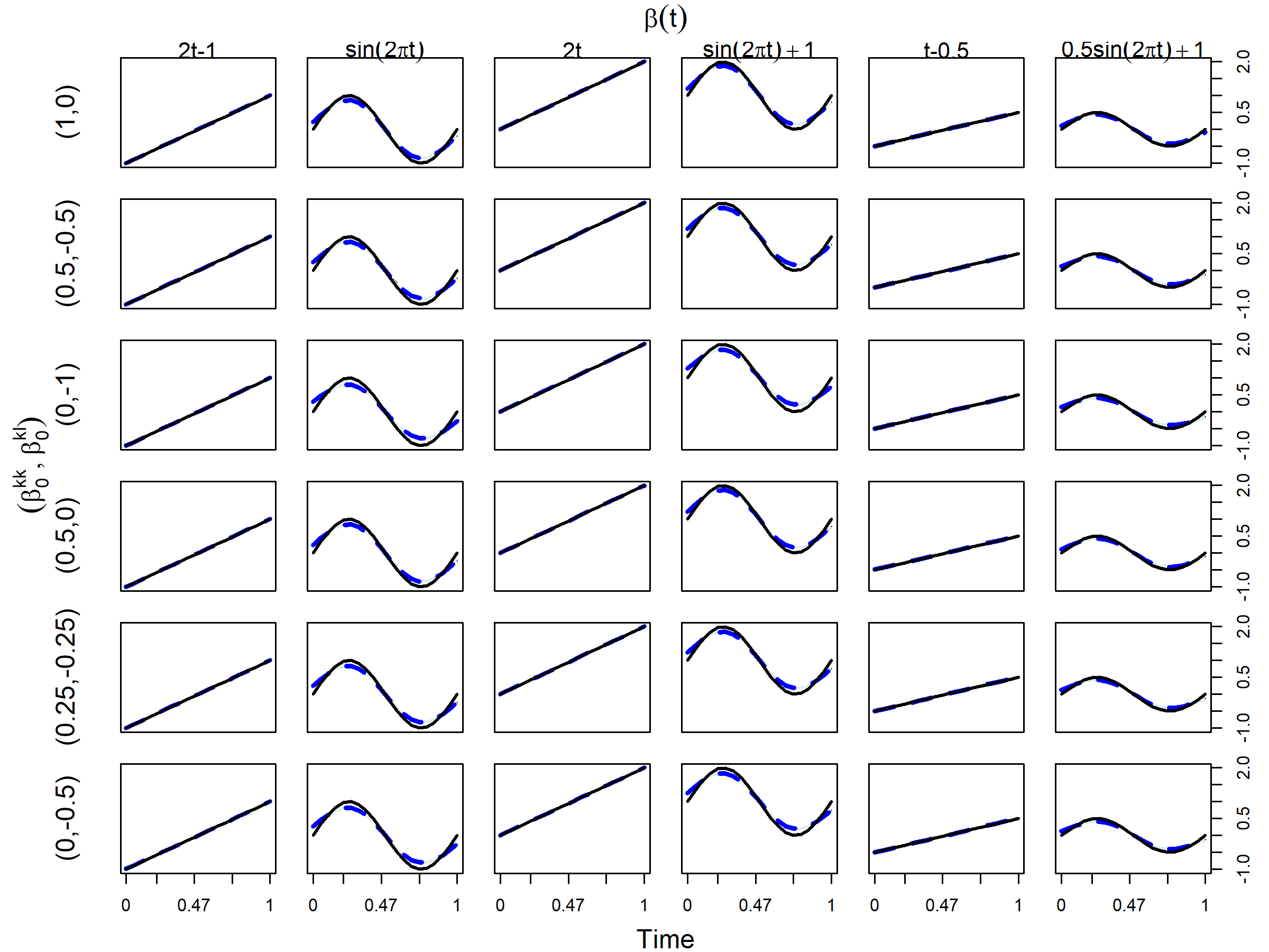
Figure 2: Estimations of $\beta(t)$ using a tuning parameter of $\lambda=0.5$ for all simulated cases with different combinations of $\beta_{0}$ and $\beta(t)$. In each panel, the black solid line is the true function $\beta(t)$; the blue dashed line is the pointwise mean of $\hat{\beta}(t)$; and the light blue shadow (hardly visible) marks the corresponding pointwise confidence band.

6 Application: International Trading

In this section, we apply the restricted Tweedie SBM to study international trading relationships among different countries and how these relationships are influenced by geographical distances. As an example, we focus on the trading of apples—not only are these data readily available from the World Bank (World Integrated Trade Solution, 2023), but one can also surmise a priori that geographical distances will likely have a substantial impact on the trading due to the heavyweight and perishable nature of this product.

From the international trading data sets provided by the World Bank (World Integrated Trade Solution, 2023), we have collected annual import and export values of edible and fresh apples among $n=66$ countries from $t_{1}=2002$ to $t_{20}=2021$. In each given year $t_{\nu}$, we observe a 66-by-66 matrix $Y(t_{\nu})$ where each cell $y_{ij}(t_{\nu})$ represents the trading value from country $i$ to country $j$ in thousands of US dollars during that year. We then average $Y(t_{\nu})$ with its transpose to ensure symmetry. Finally, a small number of entries with values ranging from 0 to 1 (i.e., total trading values less than $1,000) are thresholded to 0, and the remaining entries are logarithmically transformed. For the covariate $x_{ij}$, we use the shortest geographical distance between the two trading countries based on their borders, which we calculate using the R packages maps and geosphere.

We employ the cross-validation procedure outlined in Section 4.2 to choose the tuning parameter $\lambda$. Figure 3 displays the CV error, showing the optimal tuning parameter to be $\lambda^{*}=0.1$.

Table 6 shows how the $66$ countries are clustered into three communities by our method. Figure 4 displays the aggregated matrix, $Y(2002)+Y(2003)+\dots+Y(2021)$, with rows and columns having been permuted according to the inferred community labels. Clearly, countries in the first community trade intensively with each other and with countries in the third community. While both the second and third communities consist of countries that mainly trade with countries in the first community (rather than among themselves or between each other), the trading intensity with the first community is lot higher for the third community than it is for the second.

Figure 5 displays $\hat{\beta}(t)$, the estimated effect of geographical distances on apple trading over time. We can make three prominent observations. First, the function $\hat{\beta}(t)$ is negative over the entire time period being studied—not surprising since longer distances can only increase the cost and time of transportation, and negatively impact fresh apple trading. Next, generally speaking the magnitude of $\hat{\beta}(t)$ is decreasing over the twenty-year period, implying that the negative effect of geographical distances is diminishing. This may be attributed to more efficient method and reduced cost of shipment overtime. Finally, two relatively big “dips” in $\hat{\beta}(t)$ are clearly visible—one after the financial crisis in 2008, and another after the onset of the Covid-19 pandemic in 2020.

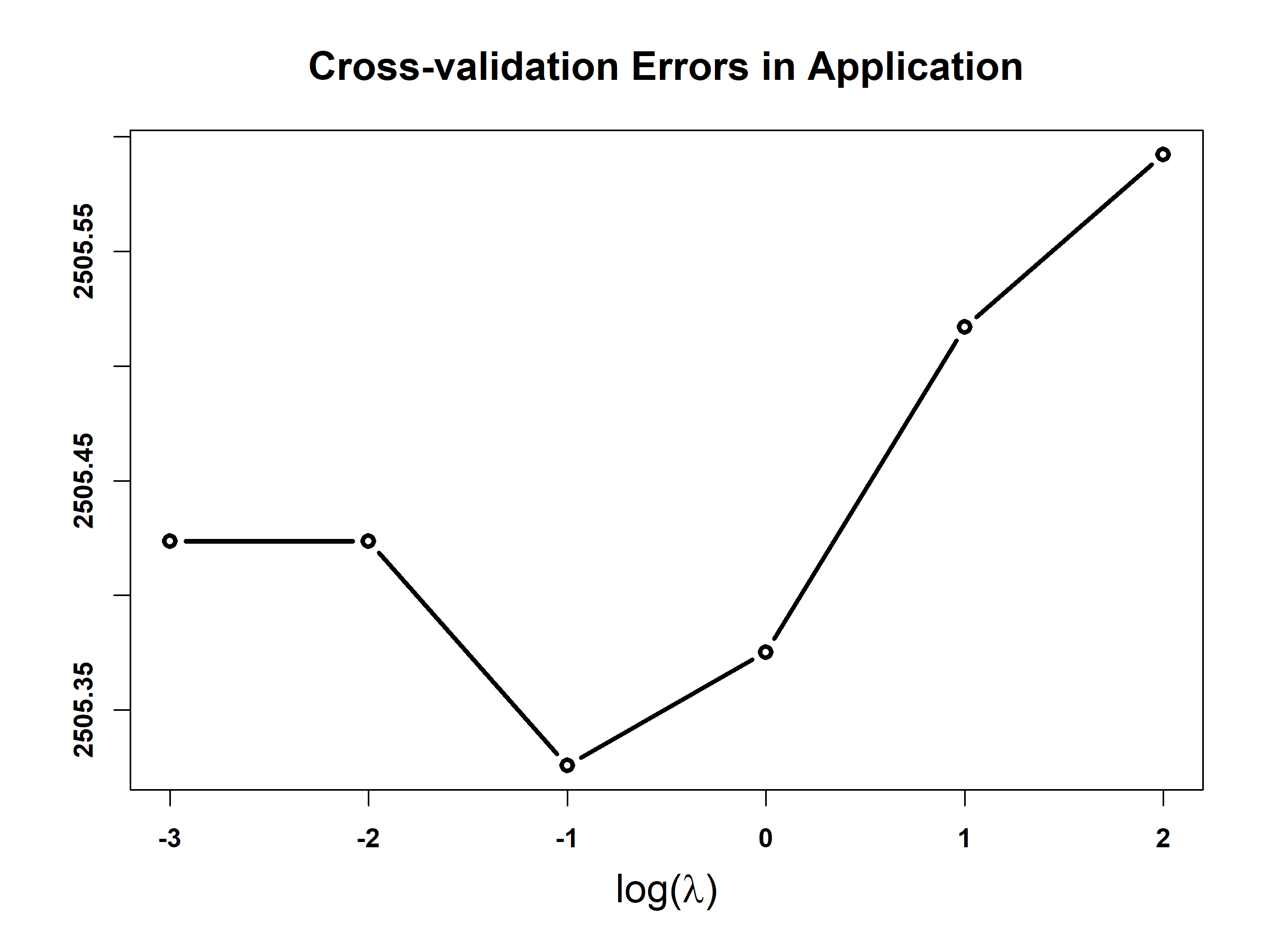
Figure 3: Cross validation errors change across a range of plausible values for the tuning parameter $\lambda$.

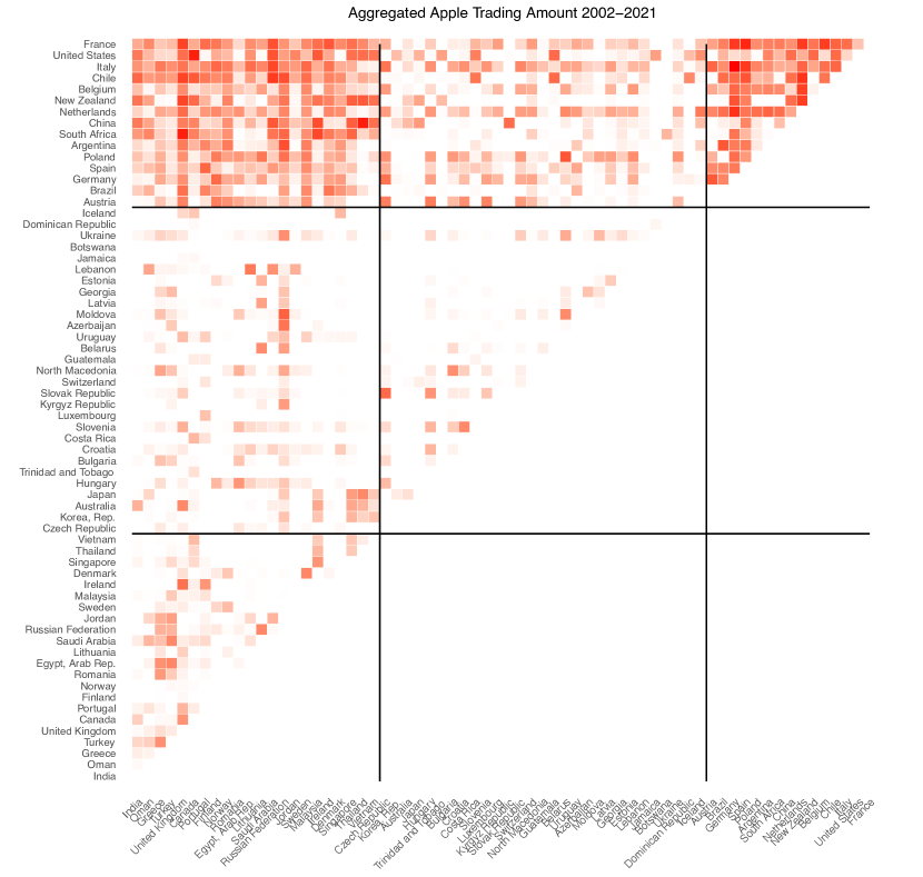
Figure 4: The (aggregated) matrix, $Y(2002)+\dots+Y(2021)$, with rows and columns having been permuted according to the inferred community labels. Due to symmetry, only the upper half of the matrix is shown, with color shadings being proportional to each entry’s respective magnitude.

Figure 5: Estimated covariate coefficient $\hat{\beta}(t)$ for $\lambda^{*}=0.1$.

Community	Country
1	France, United States, Italy, Chile, Belgium, New Zealand, Netherlands, China, South Africa, Argentina, Poland, Spain, Germany, Brazil, Austria
2	Iceland, Dominican Republic, Ukraine, Botswana, Jamaica, Lebanon, Estonia, Georgia, Latvia, Moldova, Azerbaijan, Uruguay, Belarus, Guatemala, North, Macedonia, Switzerland, Slovak, Republic, Kyrgyz Republic, Luxembourg, Slovenia, Costa Rica, Croatia, Bulgaria, Trinidad and Tobago, Hungary, Japan, Australia, Korea Rep, Czech Republic
3	Vietnam, Thailand, Singapore, Denmark, Ireland, Malaysia, Sweden, Jordan, Russian, Federation, Saudi, Arabia, Lithuania, Egypt Arab Rep., Romania, Norway, Finland, Portugal, Canada, United Kingdom, Turkey, Greece, Oman, India

Table 6: Community detection results of 66 countries.

7 Discussion

This paper generalizes the vanilla SBM by replacing the Bernoulli distribution with the restricted Tweedie distribution to accommodate non-negative zero-inflated continuous edge weights. Moreover, our model accounts for dynamic effects of nodal information. We show that as the number of nodes diverges to infinity, estimating the covariates coefficients is asymptotically irrelevant to the community labels when we maximize the likelihood function. This startling finding leads to the efficient two-step algorithm. Applying our framework to the international apple trading data provides insight into the dynamic effect of the geographic distance between countries in the trading network.

Moreover, simulation studies in Section 5 demonstrates the appealing performance of the proposed framework in clustering. This can be attributed to time independent community labels for each node, as the temporal data provide sufficient information for inferring the community labels. However, in many real world dynamic networks, the community label of each node is time dependent; it renders our current framework inapplicable. Xu and Hero (2014) and Matias and Miele (2017) proposed to use a Markov chain to address this problem, but there exist idenfitiability issues for parameters to be resolved in future work.

Appendix A MLE of $\hat{\beta}_{0}$

In this section, we provide the detailed derivation of $\hat{\beta}_{0}(\boldsymbol{\beta}(t))$ as defined in (9). Subsequently, we substitute this resulting maximum likelihood estimate of $\hat{\beta}_{0}$ back into (9), demonstrating how the equation presented in the first line of (10) is established.

The derivative of (9) with respect to $\beta_{0}^{kl}$ is given by

$$\dfrac{\partial\ell_{n}(\beta_{0},\boldsymbol{\beta}(t),\phi_{0},\rho_{0};D,z)}{\partial\beta_{0}^{kl}}=\frac{1}{\binom{n}{2}}\sum\limits_{\nu=1}^{T}\sum\limits_{1\leq i<j\leq n}\dfrac{\mathds{1}(z_{i}=k,z_{j}=l)}{\phi_{0}}\times\\ \Bigl{\{}y_{ij}(t_{\nu})\cdot\exp[(1-\rho_{0})\{\beta_{0}^{kl}+\boldsymbol{x}_{ij}^{\top}\boldsymbol{\beta}(t_{\nu})\}]-\exp[(2-\rho_{0})\{\beta_{0}^{kl}+\boldsymbol{x}_{ij}^{\top}\boldsymbol{\beta}(t_{\nu})\}]\Bigl{\}}.$$ (16)

Thus the second-order derivative is

$$\dfrac{\partial^{2}\ell_{n}(\beta_{0},\boldsymbol{\beta}(t),\phi_{0},\rho_{0};D,z)}{\partial[\beta_{0}^{kl}]^{2}}=\\ \frac{1}{\binom{n}{2}}\sum\limits_{\nu=1}^{T}\sum\limits_{1\leq i<j\leq n}\dfrac{\mathds{1}(z_{i}=k,z_{j}=l)}{\phi_{0}}\times\Bigl{\{}(1-\rho_{0})\cdot y_{ij}(t_{\nu})\cdot\exp[(1-\rho_{0})\{\beta_{0}^{kl}+\boldsymbol{x}_{ij}^{\top}\boldsymbol{\beta}(t_{\nu})\}]-\\ (2-\rho_{0})\cdot\exp[(2-\rho_{0})\{\beta_{0}^{kl}+\boldsymbol{x}_{ij}^{\top}\boldsymbol{\beta}(t_{\nu})\}]\Bigl{\}}<0.$$

Therefore, the MLE of ${\beta}_{0}^{kl}$ is given by the zero of (16) as

$$\hat{\beta}_{0}^{kl}(\boldsymbol{\beta}(t)) =\log\dfrac{\sum\limits_{\nu=1}^{T}\sum\limits_{1\leq i<j\leq n}y_{ij}(t_{\nu})\exp[(1-\rho)\boldsymbol{x}_{ij}^{\top}\boldsymbol{\beta}(t_{\nu})]\mathds{1}(z_{i}=k,z_{j}=l)}{\sum\limits_{\nu=1}^{T}\sum\limits_{1\leq i<j\leq n}\exp[(2-\rho)\boldsymbol{x}_{ij}^{\top}\boldsymbol{\beta}(t_{\nu})]\mathds{1}(z_{i}=k,z_{j}=l)}$$

$$=\log\dfrac{\hat{\theta}_{kl}}{\hat{\gamma}_{kl}}.$$

Plugging $\hat{\beta}_{0}^{kl}(\boldsymbol{\beta}(t))=\log\hat{\theta}_{kl}/\hat{\gamma}_{kl}$ into (9), we obtain the first line of the equation presented in (10):

$$\ell_{n}(\boldsymbol{\beta}(t),\phi_{0},\rho_{0};D,z)=\frac{1}{\binom{n}{2}}\sum\limits_{\nu=1}^{T}\sum\limits_{1\leq i<j\leq n}\sum\limits_{k,l=1}^{K}\dfrac{\mathds{1}(z_{i}=k,z_{j}=l)}{\phi_{0}}\times$$

$$\Bigl{[}\dfrac{y_{ij}(t_{\nu})\exp[(1-\rho_{0})\{\log\hat{\theta}_{kl}/\hat{\gamma}_{kl}+\boldsymbol{x}_{ij}^{\top}\boldsymbol{\beta}(t_{\nu})\}]}{1-\rho_{0}}-\dfrac{\exp[(2-\rho_{0})\{\log\hat{\theta}_{kl}/\hat{\gamma}_{kl}+\boldsymbol{x}_{ij}^{\top}\boldsymbol{\beta}(t_{\nu})\}]}{2-\rho_{0}}\Bigr{]}$$

$$= \frac{1}{\binom{n}{2}}\sum\limits_{k,l=1}^{K}\frac{1}{1-\rho_{0}}(\frac{\hat{\theta}_{kl}}{\hat{\gamma}_{kl}})^{1-\rho_{0}}\sum\limits_{\nu=1}^{T}\sum\limits_{1\leq i<j\leq n}\dfrac{\mathds{1}(z_{i}=k,z_{j}=l)}{\phi_{0}}\cdot y_{ij}(t_{\nu})\exp[(1-\rho_{0})\{\boldsymbol{x}_{ij}^{\top}\boldsymbol{\beta}(t_{\nu})\}]-$$

$$\frac{1}{\binom{n}{2}}\sum\limits_{k,l=1}^{K}\frac{1}{2-\rho_{0}}(\frac{\hat{\theta}_{kl}}{\hat{\gamma}_{kl}})^{2-\rho_{0}}\sum\limits_{\nu=1}^{T}\sum\limits_{1\leq i<j\leq n}\dfrac{\mathds{1}(z_{i}=k,z_{j}=l)}{\phi_{0}}\cdot\exp[(2-\rho_{0})\{\boldsymbol{x}_{ij}^{\top}\boldsymbol{\beta}(t_{\nu})\}]$$

$$= \dfrac{1}{\phi_{0}}\sum\limits_{k,l=1}^{K}\frac{1}{1-\rho_{0}}(\frac{\hat{\theta}_{kl}}{\hat{\gamma}_{kl}})^{1-\rho_{0}}\cdot\hat{\theta}_{kl}-\dfrac{1}{\phi_{0}}\sum\limits_{k,l=1}^{K}\frac{1}{2-\rho_{0}}(\frac{\hat{\theta}_{kl}}{\hat{\gamma}_{kl}})^{2-\rho_{0}}\cdot\hat{\gamma}_{kl}$$

$$= \dfrac{1}{\phi_{0}}\dfrac{1}{(1-\rho_{0})(2-\rho_{0})}\sum\limits_{k,l=1}^{K}\hat{\theta}_{kl}^{2-\rho_{0}}\cdot\hat{\gamma}_{kl}^{\rho_{0}-1}.$$

Appendix B Proof of Theorem 1

In this section, we prove Theorem 1. Before laying out the main proof, we introduce several lemmas first.

Lemma 1.

Under Conditions 3.1 to 3.2,

$$\frac{\hat{\gamma}_{kl}}{\sum\limits_{k,l}\hat{\gamma}_{kl}}=p_{k}p_{l}+o_{p}(1).$$

Proof.

Proof According to Conditions 3.1 and 3.2, $\exp[(2-\rho)x_{ij}^{\top}\beta(t)]$ and $\mathds{1}(z_{i}=k,z_{j}=l)$ are iid random variables, with mean $\gamma$ and $p_{k}p_{l}$ respectively. Specifically, $\gamma$ is a positive constant. By the weak law of large numbers, we have

$$\frac{\hat{\gamma}_{kl}}{\sum\limits_{k,l}\hat{\gamma}_{kl}} =\frac{2\sum\limits_{\nu=1}^{T}\sum\limits_{1\leq i<j\leq n}\exp[(2-\rho)\boldsymbol{x}_{ij}^{\top}\boldsymbol{\beta}(t_{\nu})]\mathds{1}(z_{i}=k,z_{j}=l)/\{n(n-1)\}}{2\sum\limits_{\nu=1}^{T}\sum\limits_{1\leq i<j\leq n}\exp[(2-\rho)\boldsymbol{x}_{ij}^{\top}\boldsymbol{\beta}(t_{\nu})]/\{n(n-1)\}}$$

$$=\frac{\gamma\cdot p_{k}p_{l}+o_{p}(1)}{\gamma+o_{p}(1)}$$

$$=p_{k}p_{l}+o_{p}(1).$$

∎

Lemma 2.

Under Conditions 3.1 to 3.2,

$$\frac{\hat{\theta}_{kl}}{\sum\limits_{k,l}\hat{\theta}_{kl}}=p_{k}p_{l}+o_{p}(1).$$

Proof.

Proof The proof is similar to that of Lemma 1. If we can show that, at each time point $t_{\nu}$, $\nu=1,\ldots,T$, $y_{ij}(t_{\nu})\exp[(1-\rho)\boldsymbol{x}_{ij}^{\top}\boldsymbol{\beta}(t_{\nu})]$ for $i,j=1,\ldots,n$ are iid with a nonzero mean, we complete the proof. For each node pair $(i,j)$, both their pairwise covariate $\boldsymbol{x}_{ij}$ and community labels $c_{i}$ and $c_{j}$ are iid. Moreover, $y_{ij}(t_{\nu})$ conditional on $x_{ij}$, $c_{i}$ and $c_{j}$ are iid as well. Therefore, $y_{ij}(t_{\nu})\exp[(1-\rho)\boldsymbol{x}_{ij}^{\top}\boldsymbol{\beta}(t_{\nu})]$ for $i,j=1,\ldots,n$ are iid, with mean

$$\mathbb{E}[y_{ij}(t_{\nu})\exp\{(1-\rho)\boldsymbol{x}_{ij}^{\top}\boldsymbol{\beta}(t_{\nu})\}] =\mathbb{E}\Bigl{(}\mathbb{E}[y_{ij}(t_{\nu})\exp\{(1-\rho)\boldsymbol{x}_{ij}^{\top}\boldsymbol{\beta}(t_{\nu})\}\mid\boldsymbol{x},\boldsymbol{c}]\Bigr{)}$$

$$=\mathbb{E}\Bigl{[}\mathbb{E}\{y_{ij}(t_{\nu})|\boldsymbol{x},\boldsymbol{c}\}\cdot\exp\{(1-\rho)\boldsymbol{x}_{ij}^{\top}\boldsymbol{\beta}(t_{\nu})\}\Bigr{]}$$

$$=\mathbb{E}\Bigl{[}\exp\{\beta_{0}^{c_{i}c_{j}}+\boldsymbol{x}_{ij}^{\top}\boldsymbol{\beta}(t_{\nu})\}\cdot\exp\{(1-\rho)\boldsymbol{x}_{ij}^{\top}\boldsymbol{\beta}(t_{\nu})\}\Bigr{]}$$

$$=\sum\limits_{k,l}\mathbb{E}\Bigl{[}\exp\left\{\beta_{0}^{kl}+(2-\rho)\boldsymbol{x}_{ij}^{\top}\boldsymbol{\beta}(t_{\nu})\right\}\Bigr{]}\cdot p_{k}p_{l}.$$

Therefore, the expectation is a nonzero constant. ∎

Next, we prove Theorem 1.

Proof.

Proof of Theorem 1 By Lemmas 1 and 2 and the continuous mapping theorem,

$$\sum\limits_{k,l}\hat{\theta}_{kl}^{2-\rho}\cdot\hat{\gamma}_{kl}^{\rho-1}$$

$$= \Bigl{[}\sum\limits_{k,l}\Bigl{(}\dfrac{\hat{\theta}_{kl}}{\sum\limits_{k,l}\hat{\theta}_{kl}}\Bigr{)}^{2-\rho}\cdot\Bigl{(}\dfrac{\hat{\gamma}_{kl}}{\sum\limits_{k,l}\hat{\gamma}_{kl}}\Bigr{)}^{\rho-1}\Bigr{]}\cdot\bigl{(}\sum\limits_{k,l}\hat{\theta}_{kl}\bigr{)}^{2-\rho}\bigl{(}\sum\limits_{k,l}\hat{\gamma}_{kl}\bigr{)}^{\rho-1}$$

$$= \Bigl{[}\sum\limits_{k,l}\Bigl{\{}(p_{k}p_{l})^{2-\rho}+o_{p}(1)\Bigr{\}}\cdot\Bigl{\{}(p_{k}p_{l})^{\rho-1}+o_{p}(1)\Bigr{\}}\Bigr{]}\cdot\bigl{(}\sum\limits_{k,l}\hat{\theta}_{kl}\bigr{)}^{2-\rho}\bigl{(}\sum\limits_{k,l}\hat{\gamma}_{kl}\bigr{)}^{\rho-1}$$

$$= \Bigl{[}\sum\limits_{k,l}\Bigl{(}p_{k}p_{l}+o_{p}(1)\Bigr{)}\Bigr{]}\cdot\bigl{(}\sum\limits_{k,l}\hat{\theta}_{kl}\bigr{)}^{2-\rho}\bigl{(}\sum\limits_{k,l}\hat{\gamma}_{kl}\bigr{)}^{\rho-1}$$

$$= \Bigl{[}1+\frac{K(K+1)}{2}o_{p}(1)\Bigr{]}\cdot\Bigl{(}\theta+o_{p}(1)\Bigr{)}^{2-\rho}\Bigl{(}\gamma+o_{p}(1)\Bigr{)}^{\rho-1}$$ (17)

$$= \theta^{2-\rho}\gamma^{\rho-1}+o_{p}(1).$$

(17) holds because $\sum_{k,l}{}\hat{\theta}_{kl}=\hat{\theta}=\theta+o_{p}(1)$ and $\sum_{k,l}{}\hat{\gamma}_{kl}=\hat{\gamma}=\gamma+o_{p}(1)$ by the weak law of large numbers. Therefore, we have

$$\dfrac{2}{n(n-1)}l_{z}(\boldsymbol{\beta}(t)) =\dfrac{1}{\phi}\dfrac{1}{(1-\rho)(2-\rho)}\sum\limits_{k,l}\hat{\theta}_{kl}^{2-\rho}\cdot\hat{\gamma}_{kl}^{\rho-1}$$

$$=\dfrac{1}{\phi}\dfrac{1}{(1-\rho)(2-\rho)}\Bigl{(}\theta^{2-\rho}\cdot\gamma^{\rho-1}+o_{p}(1)\Bigr{)}$$

$$=\dfrac{1}{\phi}\dfrac{1}{(1-\rho)(2-\rho)}\theta^{2-\rho}\cdot\gamma^{\rho-1}+o_{p}(1).$$

∎

Remark 2.

By Hölder’s inequality, we have

$$\sum\limits_{k,l}\left(\dfrac{\hat{\theta}_{kl}}{\sum\limits_{k,l}\hat{\theta}_{kl}}\right)^{2-\rho}\cdot\left(\dfrac{\hat{\gamma}_{kl}}{\sum\limits_{k,l}\hat{\gamma}_{kl}}\right)^{\rho-1}\leq\left(\sum\limits_{k,l}\dfrac{\hat{\theta}_{kl}}{\sum\limits_{k,l}\hat{\theta}_{kl}}\right)^{2-\rho}\cdot\left(\sum\limits_{k,l}\dfrac{\hat{\gamma}_{kl}}{\sum\limits_{k,l}\hat{\gamma}_{kl}}\right)^{\rho-1}=1.$$

Then, it follows

$$\dfrac{2}{n(n-1)}l_{z}(\boldsymbol{\beta}(t))\leq\dfrac{1}{\phi}\dfrac{1}{(1-\rho)(2-\rho)}\theta^{2-\rho}\cdot\gamma^{\rho-1}.$$ (18)

In fact, Lemmas 1 and 2 establish the asymptotic equality conditions, which sharpen (18) and lead to the conclusion in Theorem 1.

Appendix C Bspline estimation in Step 1

In this section, we present the details of estimating the time-varying covariate coefficient $\hat{\boldsymbol{\beta}}(t)$ in accordance to (11) as part of Step 1 in our two-step estimation process.

According to Silverman [1985] and Green and Silverman [1993], each optimal $\boldsymbol{\beta}_{u}(t),u=1,\cdots,p$ is a natural cubic spline with knots at time points where temporal data is observed. In practice, we use B-spline in the computations of smoothing splines [Hastie et al., 2009]. We use $T+4$ B-spline basis functions $\{B_{m}(t)\}_{m=1}^{T+4}$, so we can represent the scalar $\boldsymbol{\beta}_{u}(t_{\nu})$ as the $(\nu,u)-$th element in the $T-$by$-p$ matrix $\boldsymbol{B}\boldsymbol{\eta}$, where

$$\boldsymbol{B}_{T\times(T+4)}=\left[\begin{aligned} B_{1}(t_{1})&\quad\cdots\quad B_{T+4}(t_{1})\\ \vdots&\quad\ddots\quad\quad\vdots\\ B_{1}(t_{T})&\quad\cdots\quad B_{T+4}(t_{T})\\ \end{aligned}\right].$$

and $\boldsymbol{\eta}\in\mathbb{R}^{(T+4)\times p}$ is the coefficient matrix that needs to be estimated. The $p$ dimensional vector $\boldsymbol{\beta}(t_{\nu})=(\boldsymbol{B}_{\nu\cdot}\boldsymbol{\eta})^{\top}$, where $\boldsymbol{B}_{\nu\cdot}$ represents the $\nu^{th}$ row of the matrix $\boldsymbol{B}$.

If we define $\boldsymbol{\Omega}\in\mathbb{R}^{(T+4)\times(T+4)}$ where $\boldsymbol{\Omega}_{ij}=\int B_{i}^{\prime\prime}(t)B_{j}^{\prime\prime}(t)dt$ and $\boldsymbol{\lambda}=(\lambda_{1},\cdots,\lambda_{p})^{\top}$, we can solve the $(T+4)\times p$ matrix $\boldsymbol{\eta}$ by plugging $\boldsymbol{\beta}(t_{\nu})=(\boldsymbol{B}_{\nu\cdot}\boldsymbol{\eta})^{\top}$ in (11):

$$\hat{\boldsymbol{\eta}}=\operatorname*{arg\,max}_{\boldsymbol{\eta}}\\ \dfrac{1}{(1-\rho_{0})(2-\rho_{0})}\sum\limits_{k,l}\left(\sum\limits_{\nu=1}^{T}\sum\limits_{1\leq i<j\leq n}y_{ij}(t)\exp[(1-\rho_{0})\boldsymbol{B}_{\nu\cdot}\boldsymbol{\eta}x_{ij}]\mathds{1}(z_{i}=k,z_{j}=l)\right)^{2-\rho_{0}}\times\\ \left(\sum\limits_{\nu=1}^{T}\sum\limits_{1\leq i<j\leq n}\exp[(2-\rho_{0})\boldsymbol{B}_{\nu\cdot}\boldsymbol{\eta}x_{ij}]\mathds{1}(z_{i}=k,z_{j}=l)\right)^{\rho_{0}-1}-\frac{1}{2}\boldsymbol{\lambda}^{\top}\cdot diag(\boldsymbol{\eta}^{T}\boldsymbol{\Omega}\boldsymbol{\eta})$$

Once we have obtain $\hat{\boldsymbol{\eta}}$, we can calculate the estimated $\hat{\boldsymbol{\beta}}(t)$ in Step 1 by $\hat{\boldsymbol{\beta}}(t)=\boldsymbol{B}\hat{\boldsymbol{\eta}}$.

Appendix D Additional Simulation Results

D.1 Tweedie Parameters Estimated in Simulation

Although our primary interest is to estimate the covariate coefficients and infer the community labels in our model, their estimation is affected by the Tweedie parameters $\phi$ and $\rho$. In this section, we provide the simulation results regarding $\phi$ and $\rho$ in the Section 5. We report the estimated bias and standard error (SE) of the estimates of $\phi$ and $\rho$ over 50 simulation runs in Table 7,  8,  9,  10 and  11. To be more specific, we calculate the bias of the estimate $\hat{\phi}$ of $\phi$ with true value $\phi_{0}$ by $\text{bias}(\hat{\phi})=\sum_{i=1}^{50}(\hat{\phi}_{i}-\phi_{0})/50$ and $\text{SE}(\hat{\phi})=\sqrt{\sum_{i=1}^{50}(\hat{\phi}_{i}-\bar{\hat{\phi}})^{2}/49}$ where $\bar{\hat{\phi}}$ is the average of $\hat{\phi}$ over 50 simulation runs. In summary, the simulation results indicate that the estimates of $\phi$ and $\rho$ are highly accurate.

			Scenario 1		Scenario 2		Scenario 3
$\phi$	$\rho$	$n$	Bias	SE	Bias	SE	Bias	SE
$2$	$1.2$	50	0.012	0.054	0.014	0.09	0.014	0.082
		100	-0.003	0.027	0.001	0.026	0.004	0.032
	$1.5$	50	0.014	0.072	0.018	0.085	0.011	0.085
		100	0.004	0.025	0.004	0.034	0	0.032
	$1.8$	50	-0.003	0.062	-0.004	0.07	-0.001	0.056
		100	0	0.03	0.001	0.028	-0.002	0.028
$1$	$1.2$	50	0.008	0.034	0.008	0.028	0.013	0.048
		100	0.002	0.014	-0.002	0.015	-0.001	0.012
	$1.5$	50	0.008	0.039	0.006	0.033	0.01	0.033
		100	-0.001	0.018	0	0.017	0.002	0.014
	$1.8$	50	0.001	0.037	0.008	0.034	0.007	0.034
		100	0.001	0.016	0.001	0.016	-0.001	0.016
$0.5$	$1.2$	50	0.004	0.015	0	0.022	0.007	0.023
		100	0.002	0.007	0	0.008	0	0.006
	$1.5$	50	0.005	0.021	0.002	0.022	0.009	0.03
		100	0	0.01	0	0.01	-0.001	0.01
	$1.8$	50	-0.003	0.016	0.008	0.023	0.002	0.031
		100	-0.002	0.009	-0.001	0.009	-0.001	0.010

Table 7: Summary of estimated bias and standard error (SE) of estimated $\phi$ in scenario 1, 2 and 3 over 50 simulation runs.

			Scenario 1		Scenario 2		Scenario 3
$\phi$	$\rho$	$n$	Bias	SE	Bias	SE	Bias	SE
$2$	$1.2$	50	0	0	0.002	0.014	0.002	0.014
		100	0	0	0	0	0	0
	$1.5$	50	0	0	0	0	0	0
		100	0	0	0	0	0	0
	$1.8$	50	0	0	0	0	0	0
		100	0	0	0	0	0	0
$1$	$1.2$	50	0.060	0.120	0	0	0.002	0.014
		100	0	0	0	0	0	0
	$1.5$	50	-0.002	0.014	0	0	0	0
		100	0	0	0	0	0	0
	$1.8$	50	-0.002	0.014	0	0	0	0
		100	0	0	0	0	0	0
$0.5$	$1.2$	50	0	0	-0.002	0.014	0.002	0.014
		100	0	0	0	0	0	0
	$1.5$	50	0.002	0.037	-0.002	0.014	0.002	0.032
		100	0	0	0	0	0	0
	$1.8$	50	0.006	0.054	0.008	0.039	0.002	0.037
		100	0.002	0.014	0	0	0	0

Table 8: Summary of estimated bias and standard error (SE) of estimated $\rho$ in scenario 1, 2 and 3 over 50 simulation runs.

			Weak Effect ($\beta=1$)				Strong Effect ($\beta=2$)
$\phi$	$\rho$	$n$	$\hat{\phi}$		$\hat{\rho}$		$\hat{\phi}$		$\hat{\rho}$
			Bias	SE	Bias	SE	Bias	SE	Bias	SE
$2$	$1.2$	50	-0.002	0.063	0	0	0.002	0.073	0.002	0.014
		100	0.001	0.026	0	0	-0.006	0.031	0	0
	$1.5$	50	0.016	0.076	0	0	0.019	0.072	0	0
		100	0.005	0.033	0	0	0.005	0.039	0	0
	$1.8$	50	0.003	0.065	0	0	-0.007	0.066	0	0
		100	-0.002	0.032	0	0	0.004	0.035	0	0
$1$	$1.2$	50	0.003	0.03	0	0	0.002	0.032	0	0
		100	0	0.017	0	0	-0.002	0.013	0	0
	$1.5$	50	0.003	0.042	-0.002	0.014	0.009	0.052	0	0.02
		100	-0.001	0.013	0	0	0.001	0.016	0	0
	$1.8$	50	0.001	0.037	0	0	0.006	0.04	0	0
		100	-0.001	0.027	-0.002	0.014	0.003	0.02	0	0
$0.5$	$1.2$	50	0.009	0.026	0.004	0.02	0	0.014	0	0
		100	0.001	0.008	0	0	0.001	0.007	0	0
	$1.5$	50	0.003	0.027	-0.006	0.031	0.002	0.019	-0.006	0.024
		100	0	0.009	0	0	0	0.009	0	0
	$1.8$	50	0.005	0.028	-0.01	0.054	-0.002	0.025	-0.006	0.042
		100	-0.002	0.01	0	0	0.001	0.009	0	0

Table 9: Summary of estimated bias and standard error (SE) of estimated $\phi$ and $\rho$ in the static model with covariates over 50 simulation runs, with $(\beta_{0}^{kk},\beta_{0}^{kl})=(0.5,-0.5)$.

$(\beta_{0}^{kk},\beta_{0}^{kl})$	$\phi$	$\beta(t)$
		$2t-1$	$\sin(2\pi t)$	$2t$	$\sin(2\pi t)$ +1	$0.5(2t-1)$	$0.5\sin(2\pi t)$
Scenario 1	Bias	0.002	0.004	-0.001	0.007	0.003	0.004
$(1,0)$	SE	0.008	0.008	0.014	0.017	0.01	0.017
Scenario 2	Bias	0.002	0.005	0.004	0.005	0.002	0.001
$(0.5,-0.5)$	SE	0.008	0.006	0.026	0.008	0.008	0.007
Scenario 3	Bias	0.002	0.005	0	0.005	0.001	0.002
$(0,-1)$	SE	0.007	0.007	0.007	0.009	0.007	0.009
Scenario 4	Bias	0.001	0.003	0.002	0.004	0.001	0.001
$(0.5,0)$	SE	0.007	0.007	0.007	0.006	0.007	0.007
Scenario 5	Bias	0.001	0.004	0.002	0.005	0.002	0.001
$(0.25,-0.25)$	SE	0.007	0.008	0.007	0.008	0.008	0.007
Scenario 6	Bias	0	0.004	0.001	0.006	0	0.006
$(0,-0.5)$	SE	0.008	0.007	0.009	0.007	0.007	0.032

Table 10: Summary of estimated bias and standard error (SE) of estimated $\phi$ (with true value $1$) in the time-varying model over 50 simulation runs (using $\lambda=0.5$).

$(\beta_{0}^{kk},\beta_{0}^{kl})$	$\rho$	$\beta(t)$
		$2t-1$	$\sin(2\pi t)$	$2t$	$\sin(2\pi t)$ +1	$0.5(2t-1)$	$0.5\sin(2\pi t)$
Scenario 1	Bias	0	0	-0.002	0.002	0	0.002
$(1,0)$	SE	0	0	0.014	0.014	0	0.014
Scenario 2	Bias	0	0	0.002	0	0	0
$(0.5,-0.5)$	SE	0	0	0.014	0	0	0
Scenario 3	Bias	0	0	0	0	0	0
$(0,-1)$	SE	0	0	0	0	0	0
Scenario 4	Bias	0	0	0	0	0	0
$(0.5,0)$	SE	0	0	0	0	0	0
Scenario 5	Bias	0	0	0	0	0	0
$(0.25,-0.25)$	SE	0	0	0	0	0	0
Scenario 6	Bias	0	0	0	0	0	0.002
$(0,-0.5)$	SE	0	0	0	0	0	0.014

Table 11: Summary of estimated bias and standard error (SE) of estimated $\rho$ (with true value $1.5$) in the time-varying model over 50 simulation runs (using $\lambda=0.5$).

D.2 Sensitivity Analysis of Tuning Parameters in TV-TSBM

In this section, we apply the TV-TSBM on two $\lambda$ values of 1 and 0.1 respectively to conduct the sensitivity analysis of the simulation in Section 5.3.

By and large, the clustering outcomes across the three distinct tuning parameters measured by the NMI are relatively close, and all indicate high-quality clustering. With increasing $\lambda$ values, the curvature of the estimated $\hat{\beta}(t)$ diminishes. Consequently, when the true curve $\beta(t)$ is linear, larger values of $\lambda$ yield smaller errors in estimating $\hat{\beta}(t)$. Vice versa, a smaller $\lambda$ leads to a better estimation of $\hat{\beta}(t)$ when the underlying curve is a sine function. In summary, the consistent clustering outcomes across various distinct $\lambda$ values, coupled with the choice of a moderately penalized smoothness, substantiates the rationale behind adopting $0.5$ as the preferred value for $\lambda$.

$(\beta_{0}^{kk},\beta_{0}^{kl})$		$\beta(t)$
		$2t-1$	$\sin(2\pi t)$	$2t$	$\sin(2\pi t)$ +1	$0.5(2t-1)$	$0.5\sin(2\pi t)$
Scenario 1	NMI	1 (0)	1 (0)	1 (0)	1 (0)	0.996 (0.004)	1 (0)
$(1,0)$	$\text{Err}(\hat{\beta}(t))$	0.004 (0)	0.041 (0)	0.004 (0)	0.040 (0)	0.004 (0)	0.021 (0)
Scenario 2	NMI	1 (0)	1 (0)	1 (0)	1 (0)	1 (0)	1 (0)
$(0.5,-0.5)$	$\text{Err}(\hat{\beta}(t))$	0.004 (0)	0.048 (0)	0.005 (0)	0.046 (0)	0.005 (0)	0.024 (0)
Scenario 3	NMI	1 (0)	1 (0)	1 (0)	1 (0)	1 (0)	1 (0)
$(0,-1)$	$\text{Err}(\hat{\beta}(t))$	0.005 (0)	0.055 (0)	0.005 (0)	0.053 (0)	0.006 (0)	0.028 (0)
Scenario 4	NMI	0.996 (0.004)	1 (0)	1 (0)	1 (0)	1 (0)	1 (0)
$(0.5,0)$	$\text{Err}(\hat{\beta}(t))$	0.004 (0)	0.045 (0)	0.004 (0)	0.043 (0)	0.004 (0)	0.023 (0)
Scenario 5	NMI	1 (0)	1 (0)	1 (0)	1 (0)	1 (0)	1 (0)
$(0.25,-0.25)$	$\text{Err}(\hat{\beta}(t))$	0.004 (0)	0.048 (0)	0.004 (0)	0.046 (0)	0.004 (0)	0.024 (0)
Scenario 6	NMI	1 (0)	0.996 (0.004)	1 (0)	1 (0)	1 (0)	0.996 (0.004)
$(0,-0.5)$	$\text{Err}(\hat{\beta}(t))$	0.005 (0)	0.052 (0)	0.004 (0)	0.050 (0)	0.005 (0)	0.026 (0)

Table 12: Summary of clustering and estimation performance (using $\lambda=1$) from the time-varying model over 50 simulation runs, with $\phi=1$, $\rho=1.5$ and $n=50$.

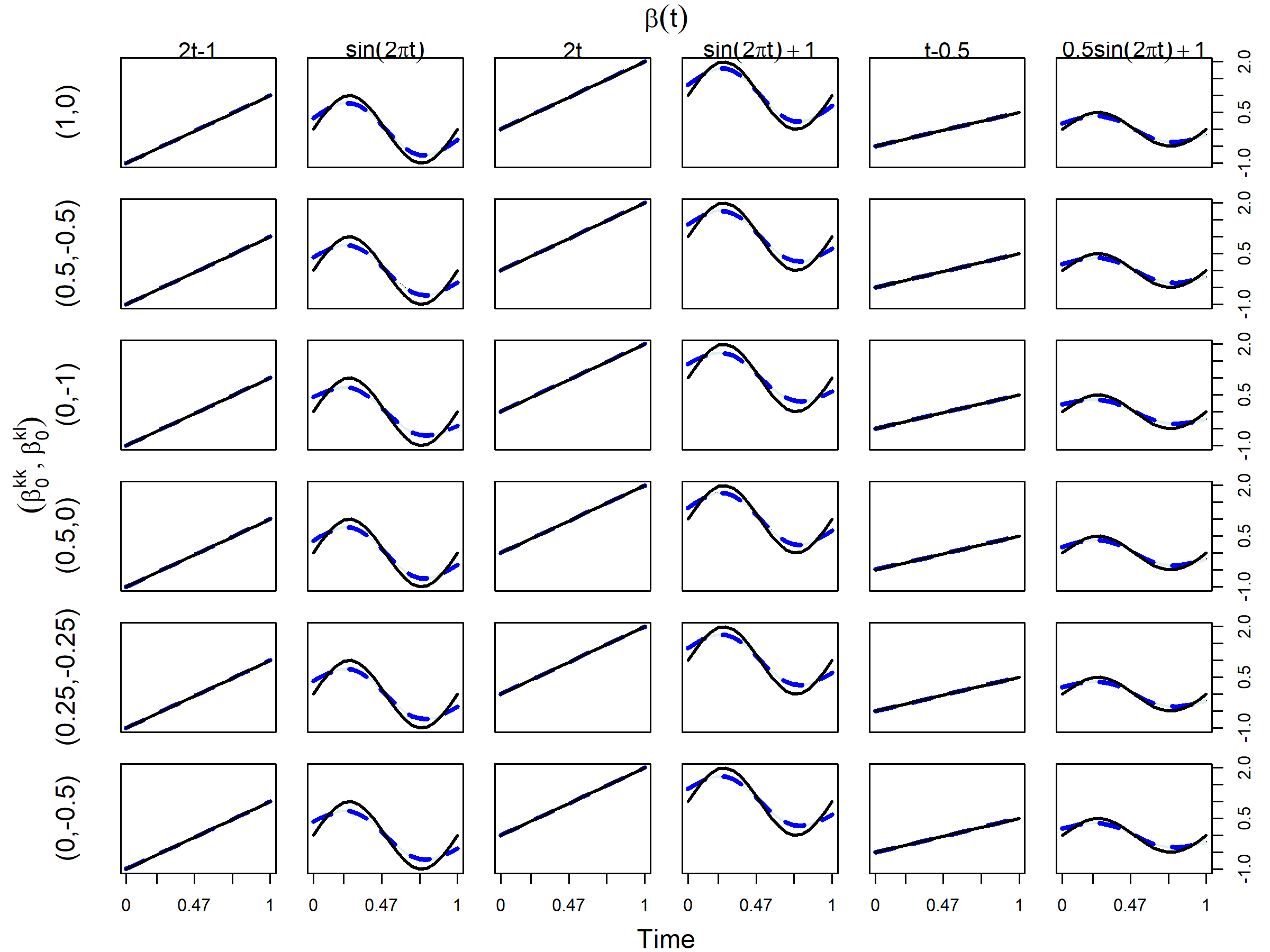
Figure 6: Estimations of the time-varying coefficients for 36 designs with $\lambda=1$, i.e. six block matrices by six functions for $\beta(t)$. In each panel, the black solid line represents the true $\beta(t)$ while the blue dashed line denotes the mean curve of $\hat{\beta}(t)$ and the light blue shadow marks the corresponding confidence band.

$(\beta_{0}^{kk},\beta_{0}^{kl})$		$\beta(t)$
		$2t-1$	$\sin(2\pi t)$	$2t$	$\sin(2\pi t)$ +1	$0.5(2t-1)$	$0.5\sin(2\pi t)$
Scenario 1	NMI	1 (0)	1 (0)	1 (0)	1 (0)	0.996 (0.004)	1 (0)
$(1,0)$	$\text{Err}(\hat{\beta}(t))$	0.005 (0)	0.008 (0)	0.005 (0)	0.008 (0)	0.005 (0)	0.006 (0)
Scenario 2	NMI	1 (0)	1 (0)	1 (0)	1 (0)	1 (0)	1 (0)
$(0.5,-0.5)$	$\text{Err}(\hat{\beta}(t))$	0.005 (0)	0.009 (0)	0.006 (0)	0.009 (0)	0.006 (0)	0.007 (0)
Scenario 3	NMI	1 (0)	1 (0)	1 (0)	0.996 (0.004)	1 (0)	1 (0)
$(0,-1)$	$\text{Err}(\hat{\beta}(t))$	0.006 (0)	0.012 (0)	0.006 (0)	0.011 (0)	0.007 (0)	0.008 (0)
Scenario 4	NMI	0.996 (0.004)	1 (0)	1 (0)	1 (0)	1 (0)	1 (0)
$(0.5,0)$	$\text{Err}(\hat{\beta}(t))$	0.005 (0)	0.009 (0)	0.006 (0)	0.008 (0)	0.006 (0)	0.007 (0)
Scenario 5	NMI	1 (0)	1 (0)	1 (0)	1 (0)	1 (0)	1 (0)
$(0.25,-0.25)$	$\text{Err}(\hat{\beta}(t))$	0.006 (0)	0.009 (0)	0.005 (0)	0.009 (0)	0.005 (0)	0.007 (0)
Scenario 6	NMI	1 (0)	1 (0)	1 (0)	0.996 (0.004)	1 (0)	0.996 (0.004)
$(0,-0.5)$	$\text{Err}(\hat{\beta}(t))$	0.006 (0)	0.010 (0)	0.006 (0)	0.010 (0)	0.006 (0)	0.007 (0)

Table 13: Summary of clustering and estimation performance (using $\lambda=0.1$) from the time-varying model over 50 simulation runs, with $\phi=1$, $\rho=1.5$ and $n=50$.

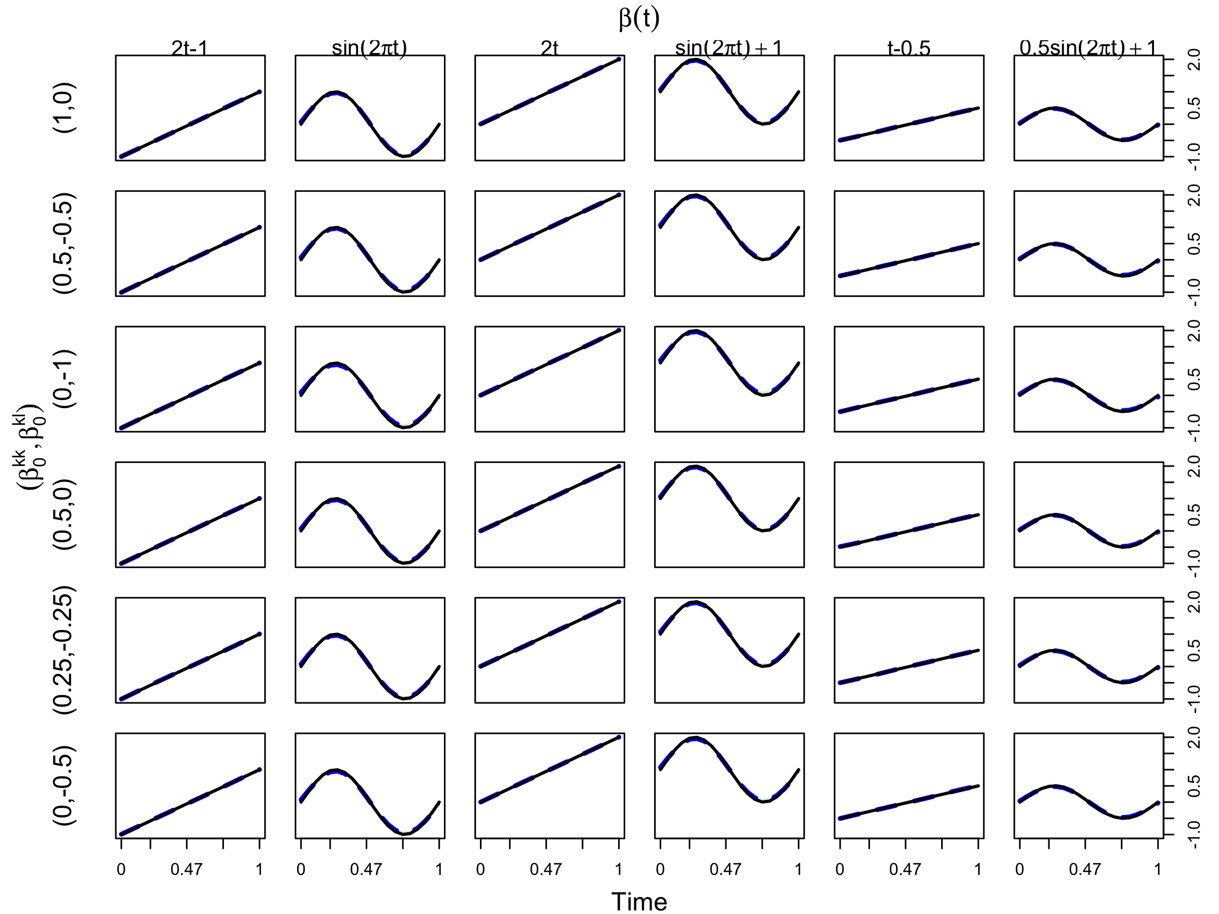
Figure 7: Estimations of the time-varying coefficients for 36 designs with $\lambda=0.1$, i.e. six block matrices by six functions for $\beta(t)$. In each panel, the black solid line represents the true $\beta(t)$ while the blue dashed line denotes the mean curve of $\hat{\beta}(t)$ and the light blue shadow marks the corresponding confidence band.

References

- Aicher et al. [2013] Christopher Aicher, Abigail Z Jacobs, and Aaron Clauset. Adapting the stochastic block model to edge-weighted networks. In ICML Workshop on Structured Learning (SLG), 2013.
- Aicher et al. [2015] Christopher Aicher, Abigail Z Jacobs, and Aaron Clauset. Learning latent block structure in weighted networks. Journal of Complex Networks, 3(2):221–248, 2015.
- Bakhthemmat and Izadi [2021] Ali Bakhthemmat and Mohammad Izadi. Communities detection for advertising by futuristic greedy method with clustering approach. Big Data, 9(1):22–40, 2021.
- Bedi and Sharma [2016] Punam Bedi and Chhavi Sharma. Community detection in social networks. Wiley Interdisciplinary Reviews: Data Mining and Knowledge Discovery, 6(3):115–135, 2016.
- Bhattacharjee et al. [2020] Monika Bhattacharjee, Moulinath Banerjee, and George Michailidis. Change point estimation in a dynamic stochastic block model. Journal of Machine Learning Research, 21(107):1–59, 2020.
- Chen and Mo [2022] Yan Chen and Dongxu Mo. Community detection for multilayer weighted networks. Information Sciences, 595:119–141, 2022.
- Choi et al. [2012] David S Choi, Patrick J Wolfe, and Edoardo M Airoldi. Stochastic blockmodels with a growing number of classes. Biometrika, 99(2):273–284, 2012.
- Danon et al. [2005] Leon Danon, Albert Diaz-Guilera, Jordi Duch, and Alex Arenas. Comparing community structure identification. Journal of Statistical Mechanics: Theory and Experiment, 2005(09):P09008, 2005.
- Dunn and Smyth [2005] Peter K Dunn and Gordon K Smyth. Series evaluation of Tweedie exponential dispersion model densities. Statistics and Computing, 15(4):267–280, 2005.
- Dunn and Smyth [2008] Peter K Dunn and Gordon K Smyth. Evaluation of tweedie exponential dispersion model densities by Fourier inversion. Statistics and Computing, 18(1):73–86, 2008.
- Fu et al. [2009] Wenjie Fu, Le Song, and Eric P Xing. Dynamic mixed membership blockmodel for evolving networks. In Proceedings of the 26th Annual International Conference on Machine Learning, pages 329–336, 2009.
- Gasparetti et al. [2021] Fabio Gasparetti, Giuseppe Sansonetti, and Alessandro Micarelli. Community detection in social recommender systems: a survey. Applied Intelligence, 51(6):3975–3995, 2021.
- Green and Silverman [1993] Peter J Green and Bernard W Silverman. Nonparametric Regression and Generalized Linear Models: a Roughness Penalty Approach. Chapman and Hall, New York, 1993.
- Guerrero-Solé [2017] Frederic Guerrero-Solé. Community detection in political discussions on twitter: An application of the retweet overlap network method to the Catalan process toward independence. Social Science Computer Review, 35(2):244–261, 2017.
- Haj et al. [2022] Abir El Haj, Yousri Slaoui, Pierre-Yves Louis, and Zaher Khraibani. Estimation in a binomial stochastic blockmodel for a weighted graph by a variational expectation maximization algorithm. Communications in Statistics-Simulation and Computation, 51(8):4450–4469, 2022.
- Hastie et al. [2009] Trevor Hastie, Robert Tibshirani, Jerome H Friedman, and Jerome H Friedman. The Elements of Statistical Learning: Data Mining, Inference, and Prediction. Springer, New York, 2 edition, 2009.
- Hoff et al. [2002] Peter D Hoff, Adrian E Raftery, and Mark S Handcock. Latent space approaches to social network analysis. Journal of the American Statistical Association, 97(460):1090–1098, 2002.
- Holland et al. [1983] Paul W Holland, Kathryn Blackmond Laskey, and Samuel Leinhardt. Stochastic blockmodels: First steps. Social Networks, 5(2):109–137, 1983.
- Huang et al. [2023] Sihan Huang, Jiajin Sun, and Yang Feng. PCABM: Pairwise covariates-adjusted block model for community detection. Journal of the American Statistical Association, 0(0):1–26, 2023.
- Lee and Wilkinson [2019] Clement Lee and Darren J Wilkinson. A review of stochastic block models and extensions for graph clustering. Applied Network Science, 4(1):1–50, 2019.
- Lian et al. [2023] Yi Lian, Archer Yi Yang, Boxiang Wang, Peng Shi, and Robert William Platt. A Tweedie compound Poisson model in reproducing kernel Hilbert space. Technometrics, 65(2):281–295, 2023.
- Lu et al. [2018] Zhenqi Lu, Johan Wahlström, and Arye Nehorai. Community detection in complex networks via clique conductance. Scientific Reports, 8(1):1–16, 2018.
- Ludkin [2020] Matthew Ludkin. Inference for a generalised stochastic block model with unknown number of blocks and non-conjugate edge models. Computational Statistics & Data Analysis, 152:107051, 2020.
- Ma et al. [2020] Zhuang Ma, Zongming Ma, and Hongsong Yuan. Universal latent space model fitting for large networks with edge covariates. Journal of Machine Learning Research, 21(4):1–67, 2020.
- MacDonald et al. [2022] Peter W MacDonald, Elizaveta Levina, and Ji Zhu. Latent space models for multiplex networks with shared structure. Biometrika, 109(3):683–706, 2022.
- Mariadassou et al. [2010] Mahendra Mariadassou, Stéphane Robin, and Corinne Vacher. Uncovering latent structure in valued graphs: a variational approach. The Annals of Applied Statistics, 4(2):715–742, 2010.
- Matias and Miele [2017] Catherine Matias and Vincent Miele. Statistical clustering of temporal networks through a dynamic stochastic block model. Journal of the Royal Statistical Society. Series B., 79(4):1119–1141, 2017. ISSN 1369-7412.
- Motalebi et al. [2021] Narges Motalebi, Nathaniel T. Stevens, and Stefan H. Steiner. Hurdle blockmodels for sparse network modeling. The American Statistician, 75(4):383–393, 2021.
- Ng and Murphy [2021] Tin Lok James Ng and Thomas Brendan Murphy. Weighted stochastic block model. Statistical Methods & Applications, 30:1365–1398, 2021.
- Peixoto [2018] Tiago P Peixoto. Nonparametric weighted stochastic block models. Physical Review E, 97(1):012306, 2018.
- Roy et al. [2019] Sandipan Roy, Yves Atchadé, and George Michailidis. Likelihood inference for large scale stochastic blockmodels with covariates based on a divide-and-conquer parallelizable algorithm with communication. Journal of Computational and Graphical Statistics, 28(3):609–619, 2019.
- Silverman [1985] Bernhard W Silverman. Some aspects of the spline smoothing approach to non-parametric regression curve fitting. Journal of the Royal Statistical Society: Series B (Methodological), 47(1):1–21, 1985.
- Tallberg [2004] Christian Tallberg. A Bayesian approach to modeling stochastic blockstructures with covariates. Journal of Mathematical Sociology, 29(1):1–23, 2004.
- Tweedie [1984] Maurice CK Tweedie. An index which distinguishes between some important exponential families. In Statistics: Applications and New Directions: Proc. Indian Statistical Institute Golden Jubilee International Conference, volume 579, pages 579–604, 1984.
- Vu et al. [2013] Duy Q Vu, David R Hunter, and Michael Schweinberger. Model-based clustering of large networks. The Annals of Applied Statistics, 7(2):1010, 2013.
- World Integrated Trade Solution [2023] World Integrated Trade Solution. International merchandise trade, tariff and non-tariff measures (NTM) data. https://wits.worldbank.org/, 2023.
- Xin et al. [2017] Lu Xin, Mu Zhu, and Hugh Chipman. A continuous-time stochastic block model for basketball networks. The Annals of Applied Statistics, 11(2):553–597, 2017.
- Xing et al. [2010] Eric P Xing, Wenjie Fu, and Le Song. A state-space mixed membership blockmodel for dynamic network tomography. The Annals of Applied Statistics, 4(2):535–566, 2010.
- Xu and Hero [2014] Kevin S Xu and Alfred O Hero. Dynamic stochastic blockmodels for time-evolving social networks. IEEE Journal of Selected Topics in Signal Processing, 8(4):552–562, 2014.
- Yang et al. [2011] Tianbao Yang, Yun Chi, Shenghuo Zhu, Yihong Gong, and Rong Jin. Detecting communities and their evolutions in dynamic social networks—a bayesian approach. Machine Learning, 82(2):157–189, 2011.
- Zhang et al. [2020] Jingfei Zhang, Will Wei Sun, and Lexin Li. Mixed-effect time-varying network model and application in brain connectivity analysis. Journal of the American Statistical Association, 115(532):2022–2036, 2020. ISSN 0162-1459.