Reuse Kernels or Activations? A Flexible Dataflow for Low-latency Spectral CNN Acceleration

Abstract.

Spectral-domain CNNs have been shown to be more efficient than traditional spatial CNNs in terms of reducing computation complexity. However they come with a ‘kernel explosion’ problem that, even after compression (pruning), imposes a high memory burden and off-chip bandwidth requirement for kernel access. This creates a performance gap between the potential acceleration offered by compression and actual FPGA implementation performance, especially for low-latency CNN inference. In this paper, we develop a principled approach to overcoming this performance gap and designing a low-latency, low-bandwidth, spectral sparse CNN accelerator on FPGAs. First, we analyze the bandwidth-storage tradeoff of sparse convolutional layers and locate communication bottlenecks. We then develop a dataflow for flexibly optimizing data reuse in different layers to minimize off-chip communication. Finally, we propose a novel scheduling algorithm to optimally schedule the on-chip memory access of multiple sparse kernels and minimize read conflicts. On a state-of-the-art FPGA platform, our design reduces data transfers by 42% with DSP utilization up to 90% and achieves inference latency of 9 ms for VGG16, compared to the baseline state-of-the-art latency of 68 ms.

1. Introduction

Convolutional Neural Networks (CNNs)(Krizhevsky et al., 2012; Simonyan and Zisserman, 2014; Szegedy et al., 2015; He et al., 2016) are a popular choice for FPGA acceleration due to their widespread utility in tasks such as classification, detection(Ren et al., 2015) and segmentation(Long et al., 2015). Accelerating CNNs on current hardware platforms brings about several major challenges: (1) model weights in the convolutional and fully-connected layers, as well as intermediate activations impose a large memory overhead; (2) convolution operations use large-scale floating-point computations, performance is thus bounded by available computing resources; (3) large data transfers between on- and off-chip memory impacts latency, throughput and total power consumption. These issues become even more critical for edge devices with only limited memory and computing capacity.

Given the large number of potentially redundant operations, compression (of the CNN model) can significantly reduce memory and computation overheads, and so is a widely accepted technique for improving efficiency. Among such methods, pruning can deliver more than $20\times$ compression(Zhang et al., 2018b), while still maintaining high accuracy. Quantization supports traditional model operations and data access patterns, but could suffer from high accuracy drop. Another alternative is frequency domain transformation; (Zhang and Prasanna, 2017; Zeng et al., 2018) convert CNNs to the spectral domain to accelerate computation without sacrificing accuracy. These come at a cost - enlarged spectral kernels and complex numbers require vastly more memory and communication bandwidth, causing spectral CNNs to be communication-bounded rather than computation-bounded. To alleviate these issues in spectral CNNs, (Niu et al., 2019) uses an ADMM (Boyd et al., 2011) based pruning method to compress spectral convolutional layers and achieve a high (uniform) compression ratio ($\sim\!4\times$) for all kernels.

Given these advances in compression efficiency, the major challenge (for both spatial and spectral CNNs) now becomes addressing the performance gap - how to port these efficiency gains across to the actual hardware platform implementation. This requires careful design-space exploration and optimization. For example, while the uniform (across kernels) compression ratio of (Niu et al., 2019) reduces load imbalance issues in sparse tensor operation, the problem of irregular data access still remains. This performance gap becomes especially critical for CNNs used in real-time machine learning applications on edge devices, such as face recognition(Amos et al., 2016), autonomous driving(Yaqoob et al., 2019) etc. In particular, computation and communication implementation overheads, unless mitigated through careful design optimizations for effectively utilizing bandwidth and minimizing latency, can severely impact performance under low-latency requirements (Chen et al., 2017)

Motivated by the challenge of overcoming the performance gap between model compression and efficient low-latency hardware implementation on FPGAs, this paper proposes a more efficient architecture for spectral convolution with sparse kernels to minimize data transfers and required bandwidth, as well as inference latency. We bridge this gap via a novel dataflow coupled with a (bounded, approximately-optimal) scheduling algorithm for irregular data access. We summarize our major contributions below:

• We provide a comprehensive complexity analysis of spectral convolutional layers, focusing on the on-chip storage versus bandwidth tradeoff. This analysis enables us to effectively identify the most critical bottleneck in each layer.

• We propose a flexible dataflow for choosing the optimal data reuse strategy in different spectral convolutional layers that minimizes data transfers and off-chip communication. To support this flexibility, we also design a unified architecture that can adjust dataflow on the fly.

• Leveraging the fact that multiple sparse kernels access the same input, we design an approximate exact-cover based scheduling algorithm to optimally schedule on-chip memory access with minimum read conflicts. For a given a number of input image replicas, we use our schedule to perform spectral convolution on each input tile in a minimum of clock cycles. Our scheduling algorithm assumes no pattern constraints on sparse kernels and is therefore generalizable to any set of sparse kernel inputs.

• We implement our design on a state-of-the-art FPGA platform. Using our flexible dataflow, data transfers are reduced by $42\%$ for VGG16. With our scheduling algorithm, DSP utilization reaches up to $90\%$ with only $10$ input replications for $64\%$ parallel kernels (on $4\times$ compressed VGG16).

Compared to the baseline inference latency of 68 ms for processing all sparse spectral convolutional layers[15] (at a bandwidth of 9GB/s), our design only needs 9 ms in total with a bandwidth of 12 GB/s. When baseline latency is scaled to match our performance, the required bandwidth becomes 58GB/s higher, far beyond single DDR capacity. Though our principal focus is on reducing latency, we are still able to achieve high throughput (112 fps).

2. Related Work

Model pruning(Han et al., 2015; He et al., 2017; Luo et al., 2017; Zhang et al., 2018b) aims to reduce storage for kernels, which removing redundant and insignificant connections in both convolutional and fully-connected layers. These methods either prune single connection(Han et al., 2015; Zhang et al., 2018b), or remove a group of connections, such as the whole channel(He et al., 2017), or the whole kernel(Luo et al., 2017; Zhou et al., 2019). Model Quantization(Gupta et al., 2015; Courbariaux et al., 2015; Jacob et al., 2018; Lin et al., 2016) compresses models by encoding float-point weights or activations into short-bit representations. Quantization can reduce computation complexity by converting float-point operation into integer or bit operation, while still holding regular dataflow that is friendly to hardware implementation.

Besides model compression, hardware implementation also assumes a key role in accelerating CNNs’ deployment. Current hardware platforms either fail to efficiently parallelize large-scale convolution/matrix operations(Sodani et al., 2016), or have a fixed memory and computing hierarchy which cannot fit all CNN models(Choquette et al., 2018). Facing these limitations in current hardware platforms, domain-specific architecture emerges as an effective solution for accelerating CNN inference. FPGA based architectures(Qiu et al., 2016; Zhang et al., 2018a; Mei et al., 2017; Zhang and Prasanna, 2017; Zeng et al., 2018) achieve very high throughput or low latency by tailoring its configurable resources (DSPs/BRAMs/LUTs) to certain model. In this way, each model can be quickly deployed into FPGA platforms. Along with design space exploration, performance and resources can be well-balanced. Among these works, (Qiu et al., 2016) adopts kernel-shaped PE array which processes all operations in one kernel simultaneously. High throughput on targeting model (VGG16) can be obtained, but at the cost of less configurability for different model with different kernel sizes. (Zhang et al., 2018a) views convolutional and fully-connected layers as uniformed matrix-multiplication process. In this way, a unified micro-architecture is proposed, in which dataflow for convolutional and fully-connected layers can be separately optimized to maximize FPGA computing and bandwidth utilization. Being aware of a lot of data reuses in convolutional layers, (Wei et al., 2017) proposes a systolic-array architecture which fully exploit data reuses by enabling communication among multiple processing elements (PEs).

Different from previous works, (Zhang and Prasanna, 2017) (Zeng et al., 2018) convert spatial convolution into spectral domain. By first tiling input images, then doing Fast Fourier Transform (FFT) on each input tile, they convert computational-intensive convolution operations into light-weighted Hadamard operations in spectral domain. The advantage is two fold. First, data flow in convolutional layers is being simplified with Hadamard product. Then, computation complexity is reduced without sacrificing accuracy. For example, for VGG16, computation complexity can be reduced by $3\times$ under input tile size of $8\times 8$. However, these two methods come with the serious issue of kernel memory explosion in spectral domain. For VGG16, by converting $3\times 3$ spatial kernel to $8\times 8$ complex-number kernel in spectral domain, storage increases by almost $15\times$. This issue become even more urgent if we use larger FFT size, which cause convolutional layer to be memory-bounded instead of computation-bounded. As a result, reduction in computation complexity cannot be fully exploited in hardware platforms due to high memory and communication overhead.

3. Background

Spatial CNNs, as we call, are convolutional neural networks that consist stacked conventional convolutional layers, followed by activation functions (like ReLU), then usually end with fully-connected layers. Convolutional layers are used to abstract features from inputs and combine them to further higher-level representations(Zeiler and Fergus, 2014). Given input activations $\bm{X}\in\mathbb{R}^{b\times c_{\text{in}}\times h_{\text{in}}\times w_{\text{in}}}$, and kernels $\bm{W}\in\mathbb{R}^{c_{\text{out}}\times c_{\text{in}}\times k\times k}$, outputs $\bm{Y}\in\mathbb{R}^{b\times c_{\text{out}}\times h_{\text{out}}\times w_{\text{out}}}$ can be calculated as:

(1) $$\bm{Y}=\Big{\{}\bm{Y}_{i,n}\Big{\}}=\Big{\{}\sum_{m=1}^{c_{\text{in}}}\bm{X}_{i,m}*\bm{W}_{n,m}\mid 1\leq i\leq b,1\leq n\leq c_{\text{out}}\Big{\}},$$

where $b$ denotes the batch size, $c_{\text{in}}$ and $c_{\text{out}}$ denotes #channels for input and output activations. $h_{\text{in}}$,$w_{\text{in}}$,$h_{\text{out}}$ and $w_{\text{out}}$ indicate spatial dimension of input and output activations. “$*$” is the convolution operator.

Fully-connected layers only consist normal matrix-vector operations with flattened input batch $\bm{X}\in\mathbb{R}^{b\times M}$, which compute output activations $\bm{Y}\in\mathbb{R}^{b\times N}$. Given kernel $\bm{W}\in\mathbb{R}^{M\times N}$, $\bm{Y}$ is obtained as show in Eq (2).

(2) $$\bm{Y}=\bm{X}\times\bm{W},$$

where $M$ and $N$ denotes the length of input and output activations.

Compared with fully-connected layers, convolutional layers account for most computations. For example, in VGG16, $99\%$ computations fall into convolutional layers. On the other side, convolutional layers only have $10\%$ of total parameters, which brings spatial convolutional layers to be bounded by available computing resources.

Spectral CNNs are the models that convert convolution in spatial domain into Hadamard product in spectral domain (frequency domain) with Fast Fourier Transform (FFT)(Zhang and Prasanna, 2017). To reduce complexity of FFT and simplify hardware implementation, it first breaks up inputs $\bm{X}$ into small tiles $\bm{X}^{t,s}\in\mathbb{R}^{b\times c_{\text{in}}\times h_{\text{in}}^{{}^{\prime}}\times w_{\text{in}}^{{}^{\prime}}}$, where $t,s$ denote the position in the whole image for each single tile, $h_{\text{in}}{{}^{\prime}},w_{\text{in}}{{}^{\prime}}$ is tile size. Usually $h_{\text{in}}{{}^{\prime}}$ equals $w_{\text{in}}{{}^{\prime}}$. Then given window size $K=h_{\text{in}}{{}^{\prime}}+k-1$, it applies FFT on these small tiles, getting the spectral-domain counterpart $\widetilde{\bm{X}}^{t,s}\in\mathbb{R}^{b\times c_{\text{in}}\times K\times K}$. After applying spectral kernels $\widetilde{\bm{W}}\in\mathbb{R}^{c_{\text{out}}\times c_{\text{in}}\times K\times K}$ on each tile, and accumulating along the dimension of input channels, we get spectral-domain output tiles $\widetilde{\bm{Y}}^{t,s}\in\mathbb{R}^{b\times c_{\text{out}}\times K\times K}$, as shown in Eq (3).

(3) $$\widetilde{\bm{Y}}^{t,s}=\Big{\{}\widetilde{\bm{Y}}^{t,s}_{i,n}\Big{\}}=\Big{\{}\sum_{m=1}^{c_{\text{in}}}\widetilde{\bm{X}}^{t,s}_{i,m}\circ\widetilde{\bm{W}}_{n,m}\mid 1\leq i\leq b,1\leq n\leq c_{\text{out}}\Big{\}},$$

where “$\circ$” denotes Hadamard product.

Finally, we use Invert Fast Fourier Transform (IFFT) to convert these tiles back to spatial domain, getting $\bm{Y}^{t,s}\in\mathbb{R}^{b\times c_{\text{out}}\times K\times K}$. To get spatial-domain activations for further non-linear operation (like ReLU, Pooling), we need to concatenate these tiles. Due to the sliding window operation of convolution, these output tile $\bm{Y}^{t,s}$ have some overlaps on the boundary. Hence, an operation called Overlap-and-Add (OaA) operation is applied to add and merge the overlap regions(Zhang and Prasanna, 2017).

(4) $$\bm{Y}=\bigcup_{t,s}\bm{Y}^{t,s}=\bigcup_{t,s}\mathcal{IFFT}(\widetilde{\bm{Y}}^{t,s}),$$

where “$\bigcup$” denotes operations that add and merge output tiles in the same image.

Converting CNNs into spectral domain reduces computation complexity in most convolutional layers. For VGG16, with FFT size $K=8$, computation complexity can be reduce by $2\times$ without any accuracy degradation(Zhang and Prasanna, 2017). Furthermore, Hadamard operation simplifies the dataflow in which sliding window on each input tiles can be avoided.

FPGA Acceleration for CNNs takes advantage of FPGAs to parallelize computations in CNNs and customize corresponding dataflow. Due to intrinsic parallel architecture in FPGA, convolution and matrix operations can be efficiently mapped into DSP arrays on FPGAs. The main focus on FPGA acceleration is to customize memory hierarchy so that data movement can be minimized between on- and off-chip memory and maximized in local memory buffer. Doing this, PEs can be guaranteed to reach peak performance during computing. Unlike ASICs, required on-chip memory in FPGA is mapped into the array of Block RAMs (BRAMs), in which each BRAM can store 36Kb data. The logic of controlling dataflow and computing is mapped into Look-Up Table (LUT) arrays in FPGA. Each LUT can be configured as various gate function. Hence, given available resources above ($N_{DSP}$ DSPs, $N_{BRAM}$ BRAMs, $N_{LUT}$ LUTs, as well as off-chip bandwidth $BW_{sys}$), FPGA designs are aimed to optimize certain objective function $T$ under these resource constraints

(5) opt $$T$$

subject to $$n_{DSP}\leq N_{DSP}$$

$$n_{BRAM}\leq N_{BRAM}$$

$$n_{LUT}\leq N_{LUT}$$

$$bw\leq BW_{sys}$$

where $n_{DSP},n_{BRAM},n_{LUT}$ and $bw$ are the required resources in the design. The objective function $T$ can be to maximize throughput, minimizing latency, or minimizing power consumption, etc.

Nowadays, since CNN compression techniques (pruning and quantization) are playing a key role in edge devices, FPGAs become even more important due to its powerful configurability. For example, pruned models require dedicated dataflow to address irregular data access and load imbalance, which makes the FPGA be a perfect platform to design specialized memory hierarchy to fully exercise potentials in compressed CNNs.

4. Complexity Analysis

Given enlarged spectral kernels, even in compressed spectral CNNs, memory and communication have totally different patterns compared with spatial CNNs. In edge devices, due to limited on-chip memory and bandwidth, also low-latency requirement, trade-off between buffering data and off-chip communication becomes nontrivial. Hence conducting a complexity analysis can help locate the primary bottleneck and explore new trade-offs in each spectral convolutional layer.

The complexity analysis is based on a general architecture model, in which data (inputs, outputs, kernels) are originally stored in off-chip memory, then streamed into on-chip memory. For each spectral convolutional layer, computing engine first fetches tiles of inputs and kernels, then computes Hadamard product and accumulation, finally writes output tiles to off-chip memory, as shown in Fig. 1. In the analysis, we assume each $K\times K$ spectral kernel is compressed by $\alpha$, in which only $\frac{K^{2}}{\alpha}$ values are non-zeros. In this context, we analyse the complexity from two aspects: On-chip storage, communication bandwidth.

4.1. On-chip storage

In most cases, on-chip memory resources are not capable of keeping all kernels/activations. The common technique is to tile kernels/activations, calculating partial outputs each time. In next round, we keep some kernels/activations on chip to be reused and bring some new data. Hence, different data reuse approaches require different number of BRAMs. In spectral convolutional layers, we can choose to reuse input tiles/kernels/output partial sums.

To reuse input tiles, we fix input activations on chip until they serve all kernels, while kernels are grouped to be fed into on-chip buffers. In doing this, since kernel buffers are overwritten by another group of kernels, we have to re-load them when starting operation on new input tiles. On the contrary, reusing kernels leads to an opposite dataflow in which parts of kernels are kept on chip, streaming input tiles instead. Reusing output partial sums is to keep partial sums on chip until all input channels of current tile are finished, which avoids writing and re-loading partial sums back and forth.

To give a general analysis, suppose we parallelize $N^{{}^{\prime}}$ kernels, $M^{{}^{\prime}}$ input channels, and $P^{{}^{\prime}}$ input tiles, given the fact that each BRAM can only support one concurrent access, each parallel line (kernel, input channels, input tiles) needs at least one BRAM to support parallel accesses. Besides, we also need to write partial sums to output buffer in parallel. In addition, if kernels are sparse, we need some replicas ($r$) for each input tile to support accesses to the same input tile from multiple kernels (See Sec. 5.3).

In the case of reusing kernels and output partial sums (Flow #1), we keep kernels and partial sums on chip, streaming all input tiles, the required BRAMs will be at least

(6) $$n_{BRAM}=\underbrace{rM^{{}^{\prime}}P^{{}^{\prime}}}_{\text{Input tiles}}+\underbrace{M^{{}^{\prime}}N^{{}^{\prime}}}_{\text{Kernels}}+\underbrace{N^{{}^{\prime}}P^{{}^{\prime}}\left\lceil\frac{h_{\text{in}}w_{\text{in}}\cdot K^{2}}{P^{{}^{\prime}}h_{\text{in}}{{}^{\prime}}w_{\text{in}}{{}^{\prime}}\cdot 1024}\right\rceil}_{\text{partial sums}},$$

where “$1024$” indicates memory depth for single BRAM, and “$K^{2}$” is output tile size.

On the other side, if we choose to reuse input tiles and output partial sums, streaming kernels (Flow #2), the required BRAMs will be at least

(7) $$n_{BRAM}=\underbrace{rM^{{}^{\prime}}P^{{}^{\prime}}}_{\text{Input tiles}}+\underbrace{M^{{}^{\prime}}N^{{}^{\prime}}}_{\text{Kernels}}+\underbrace{M^{{}^{\prime}}P^{{}^{\prime}}\left\lceil\frac{N\cdot K^{2}}{N^{{}^{\prime}}\cdot 1024}\right\rceil}_{\text{partial sums}},$$

If we reuse input tiles and kernels, streaming partial sums (Flow #3), $n_{BRAM}$ can be obtained as follows:

(8) $$n_{BRAM}=\min \left\{\right.\underbrace{rM^{{}^{\prime}}P^{{}^{\prime}}\left\lceil\frac{h_{\text{in}}w_{\text{in}}\cdot K^{2}}{P^{{}^{\prime}}h_{\text{in}}{{}^{\prime}}w_{\text{in}}{{}^{\prime}}\cdot 1024}\right\rceil}_{\text{Input tiles}}+\underbrace{M^{{}^{\prime}}N^{{}^{\prime}}}_{\text{Kernels}}+\underbrace{M^{{}^{\prime}}P^{{}^{\prime}}}_{\text{partial sums}},$$

$$\underbrace{rM^{{}^{\prime}}P^{{}^{\prime}}}_{\text{Input tiles}}+\underbrace{M^{{}^{\prime}}N^{{}^{\prime}}\left\lceil\frac{\frac{1}{\alpha}\cdot N\cdot K^{2}}{N^{{}^{\prime}}\cdot 1024}\right\rceil}_{\text{Kernels}}+\underbrace{M^{{}^{\prime}}P^{{}^{\prime}}}_{\text{partial sums}}\left.\right\},$$

where $\alpha$ is the compression ratio.

For some layers, $n_{BRAM}$ can be very large in certain flow, even beyond the system capacity, which are detailed in Sec 5.2. Therefore, through this analysis, we can accurately describe if certain flow is bounded by BRAMs. On the other hand, we can also find out which flow needs minimum number of BRAMs.

4.2. Communication bandwidth

Different dataflows bring different communication overhead between on- and off-chip memory. Suppose for certain spectral convolutional layer $i$, the latency is set to be $\tau_{i}$ (s),the lower bound of the required bandwidth is: $bw=\frac{\#\text{Data transfers}}{\tau_{i}}$. Off-chip communication consists of reading inputs and kernels, writing outputs, writing and re-loading partial sums. Given three dataflow above, we formulate the required bandwidth as follows:

In Flow #1, input buffer is overwritten by new input tiles after each round. If we start computation with new group of kernels, we have to re-load corresponding input tiles. Given latency $\tau_{i}$ in layer $i$, the required bandwidth is:

(9) $$bw=\underbrace{\frac{Mh_{\text{in}}w_{\text{in}}\cdot\frac{N}{N^{{}^{\prime}}}}{\tau_{i}}}_{\text{Inputs}}+\underbrace{\frac{\frac{1}{\alpha}\cdot NMK^{2}}{\tau_{i}}}_{\text{Kernels}}+\underbrace{\frac{Nh_{\text{out}}w_{\text{out}}}{\tau_{i}}}_{\text{Outputs}},$$

where “$\frac{N}{N^{{}^{\prime}}}$” means the number of times for re-loading input tiles.

In Flow #2, kernel buffer is overwritten instead. Compared with Flow #1, the main communication rests on re-loading kernels.

(10) $$bw=\underbrace{\frac{Mh_{\text{in}}w_{\text{in}}}{\tau_{i}}}_{\text{Inputs}}+\underbrace{\frac{\frac{1}{\alpha}\cdot NMK^{2}\cdot\frac{h_{\text{in}}w_{\text{in}}}{P^{{}^{\prime}}h_{\text{in}}{{}^{\prime}}w_{\text{in}}{{}^{\prime}}}}{\tau_{i}}}_{\text{Kernels}}+\underbrace{\frac{Nh_{\text{out}}w_{\text{out}}}{\tau_{i}}}_{\text{Outputs}},$$

where “$\frac{h_{\text{in}}w_{\text{in}}}{P^{{}^{\prime}}h_{\text{in}}{{}^{\prime}}w_{\text{in}}{{}^{\prime}}}$” means the number of times for re-loading kernels.

Different with Flow #1 and Flow #2, Flow #3 needs to write partial sums to off-chip memory and re-load them if needed, which stands out as the main communication overhead.

(11) $$bw=\underbrace{\frac{Mh_{\text{in}}w_{\text{in}}}{\tau_{i}}}_{\text{Inputs}}+\underbrace{\frac{\frac{1}{\alpha}\cdot NMK^{2}}{\tau_{i}}}_{\text{Kernels}}+\underbrace{\frac{Nh_{\text{out}}w_{\text{out}}\cdot 2\cdot\frac{M}{M^{{}^{\prime}}}}{\tau_{i}}}_{\text{Outputs}},$$

where “$2\cdot\frac{M}{M^{{}^{\prime}}}$” means the number of times for writing/reading partial sums.

Combining these two analyses, each layer’s overhead of both on-chip storage and communication for each dataflow is brought to the surface. Knowing the overhead, we can find an optimal dataflow, even a hybrid one which combines different flow strategies, to minimize hardware overhead, as detailed in Sec. 5.2.

5. Architecture Design

5.1. Overview

According to previous analysis, each spectral convolutional layer might prefer certain dataflow to make an optimal trade-off between memory and communication overhead. To support this flexibility, we design a unified architecture that can adjust dataflow on the fly, as shown in Fig. 1. Streaming controller decides what data (inputs, kernels, partial sums) should be reused or streamed based on each layer’s configurations (Sec. 5.2). Also, irregular data access can be well-solved by joint optimization of scheduling algorithm and supportive hardware implementation (Sec. 5.3).

The whole process is: all inputs, kernels, and outputs are originally stored in DDR memory; once FPGA kernel starts, input tiles and kernels are fed into on-chip buffer before enabling process elements (PEs); then, these tiles are converted into spectral domain by 2D FFT (kernels are already in spectral representation); then we start all parallel PEs, calculating Hadamard product and accumulating partial sums along input channels; after all input channels of current tiles are done, output tiles are converted back to spatial domain using 2D IFFT before writing into DDR memory. To reduce latency, we choose to process multiple input tiles and kernels simultaneously, and process input channels in a serial manner ($M^{{}^{\prime}}=1$) so that write conflicts can be avoided. In each round, one input tile can be reused by all $N^{{}^{\prime}}$ parallel kernels, while each kernel can be reused by $P^{{}^{\prime}}$ tiles.

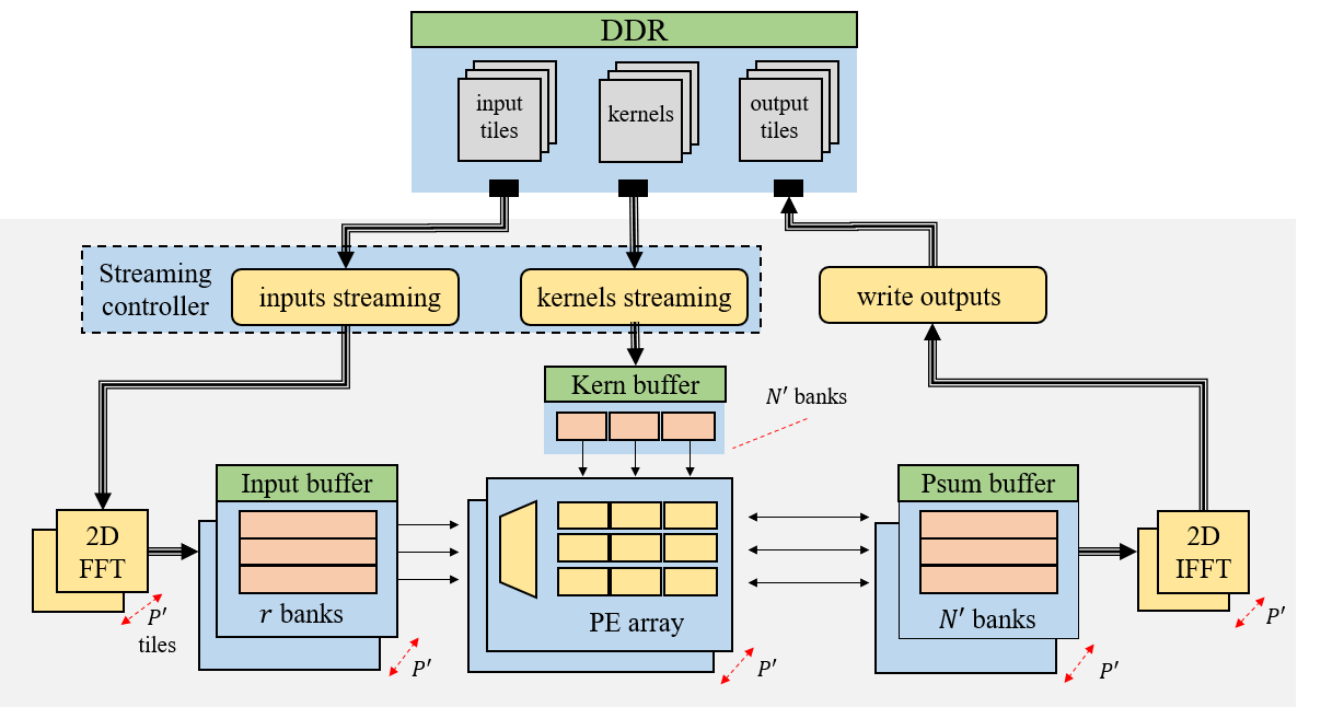
Figure 1. Overview of spectral CNN Arch.

5.2. Flexible dataflow

Keeping a fixed dataflow across all layers cannot guarantee data transfers are minimized. Based on the analysis in Sec. 4, the required on-chip memory and communication bandwidth differs among dataflows. For example, Fig. 2 shows required on-chip memory and off-chip bandwidth in three dataflows for compressed VGG16 ($\alpha=4$): Flow #1 (streaming input tiles), Flow #2 (streaming kernels), and Flow #3 (streaming partial sums).

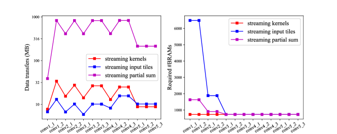
Figure 2. Complexity in VGG16(Left: Data transfers; Right: Required BRAMs)

It is easy to see that streaming input tiles (reuse kernels and partial sums) though has fewer data transfers, it requires huge number of BRAMs. On the other side, streaming kernels needs fewer BRAMs but poses higher communication overhead. Another interesting thing comes with streaming partial sums which brings no advantages at all due to its huge amount of data transfers. Similar observations also hold in other compressed networks. Inspired by this, we propose an optimization algorithm to flexibly decide #kernels should be processed before flushing corresponding input tiles, and #input tiles before flushing corresponding kernels. We call these two parameters streaming parameters: $Ns$ (kernels) and $Ps$ (input tiles). Then the required BRAMs is at least:

(12) $$n_{BRAM}=\underbrace{rP^{{}^{\prime}}}_{\text{Input tiles}}+\underbrace{N^{{}^{\prime}}\left\lceil\frac{\frac{1}{\alpha}\cdot N_{s}K^{2}}{N^{{}^{\prime}}\cdot 1024}\right\rceil}_{\text{Kernels}}+\underbrace{N^{{}^{\prime}}P^{{}^{\prime}}\left\lceil\frac{N_{s}P_{s}K^{2}}{N^{{}^{\prime}}P^{{}^{\prime}}\cdot 1024}\right\rceil}_{\text{partial sums}}.$$

The required bandwidth is at least:

(13) $$bw=\underbrace{\frac{Mh_{\text{in}}w_{\text{in}}\cdot\frac{N}{N_{s}}}{\tau_{i}}}_{\text{Inputs}}+\underbrace{\frac{\frac{1}{\alpha}NMK^{2}\cdot\frac{h_{\text{in}}w_{\text{in}}}{P_{s}h_{\text{in}}^{{}^{\prime}}w_{\text{in}}^{{}^{\prime}}}}{\tau_{i}}}_{\text{Kernels}}+\underbrace{\frac{Nh_{\text{out}}w_{\text{out}}}{\tau_{i}}}_{\text{Outputs}}.$$

Algorithm 1 Dataflow optimization algorithm

1:Compressed CNN model with compress ratio $\alpha$.

2:#parallel input tiles $P^{{}^{\prime}}$; #parallel kernels $N^{{}^{\prime}}$; streaming parameters $Ps$, $Ns$;

3:for ($P^{{}^{\prime}}$,$N^{{}^{\prime}}$) in possible arch parameters do

4:     for $lyr$ in all conv layers do

5:         Get layer parameter ($M$, $N$, $P$, $h_{\text{in}}$,$w_{\text{in}}$, $K$, $h_{\text{in}}^{{}^{\prime}}$,$w_{\text{in}}^{{}^{\prime}}$)

6:         for ($Ps$, $Ns$) in all possible streaming parameters do

7:              $n_{BRAM1}\leftarrow\text{\#BRAMs needed for }\textbf{Flow \#1}$

8:              $n_{BRAM2}\leftarrow\text{\#BRAMs needed for }\textbf{Flow \#2}$

9:              $n_{BRAM3}\leftarrow\text{\#BRAMs needed for }\textbf{Flow \#3}$

10:              Choose the flow with minimum #BRAMs

11:              $n_{BRAM}\leftarrow\min(n_{BRAM1},n_{BRAM2},n_{BRAM3})$

12:              if $n_{BRAM}<N_{BRAM}$ then

13:                  $bw\leftarrow\text{Calculate bandwidth (Eq.~{}\ref{eq::reqBWflexible})}$

14:                  if $bw<bw_{\text{min}}$ then$\triangleright$ Current streaming

15:                       $bw_{\text{min}}\leftarrow bw$

16:                       Update steaming parameter ($Ps$, $Ns$)

17:                  end if

18:              end if

19:         end for

20:         $bw_{\text{max}}\leftarrow\text{Register max bandwidth in all layers}$

21:     end for

22:     if $bw_{\text{max}}<bw_{\text{arch}}$ then$\triangleright$ Current arch

23:         $bw_{\text{arch}}\leftarrow bw_{\text{max}}$

24:         Update arch parameter ($P^{{}^{\prime}},N^{{}^{\prime}}$)

25:     end if

26:end for

Considering different architecture parameters ($P^{{}^{\prime}}$, $N^{{}^{\prime}}$) also lead to different performance, to get the optimal trade-off, we design a heuristic optimization method to find optimal settings for both architecture and streaming parameters, as shown in Alg. 1.

Given a compressed model, Alg. 1 does a heuristic search in architecture parameter space, as well as in streaming parameter space. In each layer, we fix architecture parameters ($P^{{}^{\prime}}$, $N^{{}^{\prime}}$), trying all possible streaming parameters ($Ps$, $Ns$). In each streaming setting, we choose the one with minimum required BRAMs, then calculate its bandwidth $bw$. We update the optimal streaming parameter if the resulting bandwidth $bw$ is less than previous minimum $bw_{\text{min}}$. After iterating all layers, we register the maximum bandwidth $bw_{\text{max}}$ as bandwidth requirement in current architecture setting. Finally, we choose the pair ($P^{{}^{\prime}}$, $N^{{}^{\prime}}$) and ($Ps$, $Ns$) with minimum $bw_{\text{max}}$ given a network model.

Streaming controller in Fig. 1 is designed to adjust dataflow in different layers. Streaming options are managed by a internal state machine, as shown in Fig. 3. Each time when spectral convolution is done (DONE CONV), the state machine first checks if the number of processed kernel reaches $N_{s}$. If not ($!N_{s}$), it continue reading kernels (READ KERNEL). Otherwise, when all input channels of current kernels haven’t been done ($!M_{s}$), two cases can arise: first, $P_{s}$ input image tiles have been finished, for which we need to flush all kernels and input tiles, loading input tiles and kernels from new input channel; second, we are still on the way of processing $P_{s}$ input tiles in current input channel, for which we need to load new input tiles, while kernels are already loaded. Another situation is that $M_{s}$ input channels for current $N_{s}$ kernels and $P_{s}$ tiles are done, it then starts IFFT operation (RPOC IFFT) to convert output image tiles back into spatial domain, then write to off-chip memory (WRITE OUT). At this time, we check if all kernels and input tiles are done, if not ($!(N\&P)$), we go back to read input tiles and kernels, otherwise, we complete current spectral convolutional layer (DONE).

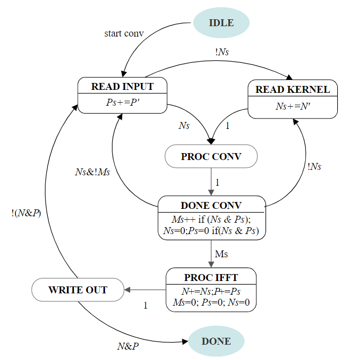
Figure 3. Streaming controller

5.3. Memory access scheduling

Memory access scheduling comes with the fact that parallel sparse kernels assume different access patterns to input tiles. As shown in Fig. 4 which is a typical case of memory access in our design, in which multiple kernels are processed in parallel, while weight values in each kernel are streamed in serial. In each cycle, each PE sends a read address to the input BRAM. After getting the input, PE multiplies it with a corresponding kernel value, then accumulate with the one in partial sums buffer (Fig. 1). Given $N^{{}^{\prime}}$ parallel kernels, at worst, one input BRAM needs to provide $N^{{}^{\prime}}$ different values in a single clock cycle, which violates BRAM’s principle of single access.

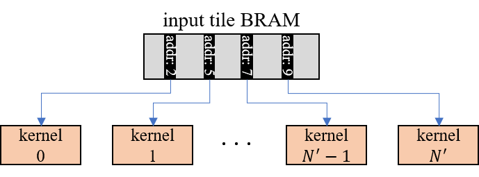
Figure 4. Sparse kernel access

To prevent multiple kernels from starving for no available inputs, we use $r$ replicas to increase throughput of input BRAMs. And noting that some kernels might access the same location, which can be served by one BRAM, the number of replicas can be smaller than $N^{{}^{\prime}}$. Given $N^{{}^{\prime}}$ sparse kernels and $r$ replicas for each input tile, in order to minimize clock cycles of Hadamard product on current $N^{{}^{\prime}}$ kernels and $P^{{}^{\prime}}$ tiles, we design a novel scheduling algorithm to optimally group read requests.

Our scheduling arises from the notion that the order of processing each value in a kernel does not matter. As long as the corresponding indices come along with the value to specify where to write corresponding result into, we can rearrange values in current kernel group in any order. The scheduling algorithm is aimed to group access addresses so that the number of distinct addresses in each read cycle is less than $r$, while the number of cycles of finishing current group of sparse kernels reach minimum. Given $N^{{}^{\prime}}$ sparse kernels, in which each kernel is represented by a format of $\left\{(val,index)\mid 0\leq index\leq K^{2}\right\}$. The number of indices in each kernel exactly equals to $\frac{K^{2}}{\alpha}$. Therefore, the scheduling can be obtained by solving the following problem: given a matrix $M$ of size $N^{\prime}\times K^{2}/\alpha$ where each row stores indices of the same kernel, rearrange values in each row to minimize $\sum_{i=1}^{K^{2}/\alpha}\lceil ID_{i}/r\rceil$, where $ID_{i}$ is the number of distinct indices in the $i^{th}$ column. we refrain from rearranging within the columns as it may result in memory conflicts in the output.

We first transform the representation into a bipartite graph, as shown in Fig. 5, in which each connection between kernel node and index node means the kernel has non-zero value in corresponding index $ID_{x}$.

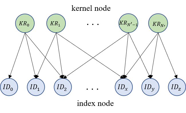
Figure 5. Bipartite presentation of sparse kernels

Based on this bipartite graph, we can construct a unit scheduling set $s_{i}=\left\{(KR_{x_{i}},ID_{x_{i}}),...,(KR_{y_{i}},ID_{y_{i}})\right\}$ that meets following constraints: (C1) elements in each set have distinct kernel nodes $KR_{x}$, which reflects the fact that only one value in each kernel can be processed in each cycle; (C2) the number of different indices $ID_{x}$ cannot exceed $r$, which enables $r$ replicas to feed all selected kernels. Each set $s_{i}$ represents one-cycle read access of $N^{{}^{\prime}}$ parallel PEs. Since kernels are shared among $P^{{}^{\prime}}$ input tiles, $s_{i}$ can be broadcast to all $P^{{}^{\prime}}$ input tiles. Ideally, we can find all welcome sets $S=\left\{s_{1},s_{2},...,s_{i},...\right\}$. Then, to get an optimal scheduling which has minimum clock cycles, we need to find the set collection $S^{*}\subset S$ which has the minimum number of sets. This is exactly an exact cover problem.

Given huge number of possible set $s_{i}$ and exact-cover problem is NP-complete, we choose to use a greedy algorithm to efficiently approximate the optimal solution, as shown in Alg. 2. In each step, we find a set $s_{i}$ that greedily leads to optimal solution. Two cases come up during searching: First, if there are a set collection $S^{{}^{\prime}}$ covering all kernel nodes, then we need to decide which sets to be chosen so that it causes minimal adverse effects on following optimization. We choose to leave as many high-degree index nodes as possible for future search since it’s easier to find a set that can cover most kernels if we have free high-degree index nodes. Therefore, we choose the set $s_{i}$ that has lower-degree index nodes, leaving high-degree nodes untouched. In the second case, if there is no such set covering all kernel nodes, we will choose the set $s_{i}$ that covers as many kernel nodes as possible, which is aimed to maximize current PEs utilization.

Algorithm 2 Scheduling algorithm

1:Compressed kernels.

2:Set collection $S^{*}=\left\{s_{1},s_{2},...,s_{i},...\right\}$ for scheduling.

3:Construct bipartite graph $G(KR,ID)$

4:while There are edges existing in $G(KR,ID)$ do

5:     Find set collection $S$ that meet above constraint C1, C2

6:     if there are sets $S^{{}^{\prime}}$ covering all kernel nodes then

7:         for set $s_{i}$ in $S^{{}^{\prime}}$ do

8:              Choose $s_{i}$ in which edges has minimum index

9:              node degree in $G(KR,ID)$

10:         end for

11:     else

12:         for set $s_{i}$ in $S$ do

13:              Choose $s_{i}$ which cover most kernel nodes in

14:              $G(KR,ID)$

15:         end for

16:     end if

17:     Push selected set $s_{i}$ into $S^{*}$

18:     Delete edges in selected set $s_{i}$ from $G(KR,ID)$

19:end while

After getting the scheduling list, to efficiently access values in kernel and replica buffers, we break $S^{*}$ into two parts, INDEX table and Value table. For each $s_{i}\in S^{*}$, we collect the unique indices, storing them into INDEX table; we store weights and corresponding selection signal $sel$ into VALUE table, as shown in Fig. 6. During hardware implementation, we first read these indices ($rep_{0}$,$rep_{1}$) and value tables, then we use these indices to read necessary inputs at current cycle, then we use sel signal in value tables to route inputs into corresponding PEs. Furthermore, in some cases, some kernels might be inactive due to too many unique addresses in current cycle. Therefore, we use valid signal to indicate whether we should feed certain kernels or not.

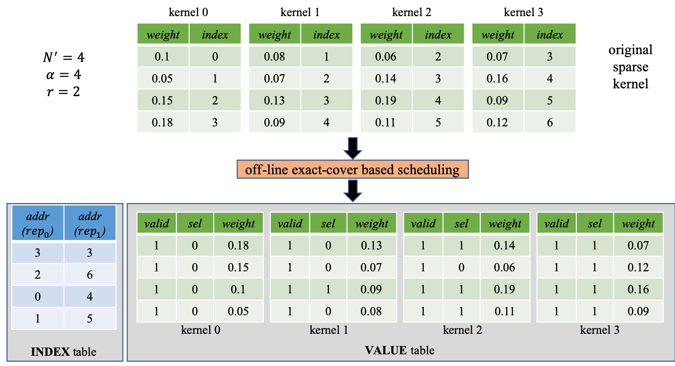
Figure 6. Storage arrangement for sparse kernels

6. Design Evaluation

The fundamental objective in this paper is to reduce communication overhead brought by enlarged spectral kernels and minimize read conflicts when multiple sparse kernels access input tile in one single BRAM. In this section, we use VGG16 to show: (1) how our dataflow optimization technique achieves an optimal trade-off between bandwidth and BRAM usage; (2) how exact-cover based scheduling method improves PE utilization. Sec. 6.1 covers detailed results of BRAM usage and communication bandwidth using various dataflow techniques. Then in Sec. 6.2, we employ kernels with different patterns to show exact-cover based scheduling method delivers higher PE utilization. FPGA implementation results are shown in Sec. 6.3.

We use a heterogeneous CPU-FPGA platform, Xilinx Alveo U200, in which operations like OaA(Zhang and Prasanna, 2017), ReLU, Pooling, fully-connected layers are offloaded to CPU, while FPGA is dedicated to spectral convolutional layers. 16-bit fix-point (FX) number is adopted during computing. RTL code is synthesized and implemented in Xilinx Vivado 2018.3, then integrated into OpenCL environment.

6.1. Data transfers

We use the amount of transferred data between on- and off-chip memory as the metric to compare communication overhead in different dataflows. Required bandwidth can be easily obtained given latency $\tau_{i}$ on each layer.

Table1 shows the optimal architecture and streaming parameters for VGG16 given compression ratio $\alpha=4$. Since the first layer (conv1_1) has negligible computations, we omit it during dataflow optimization. Given these parameters for each layer, and based on previous complexity analysis in Sec. 4 and Sec. 5.2, we can compare this optimized flow Flow opt with Flow #1 (streaming kernels) and Flow #2 (streaming input tiles) in terms of BRAM usage and data transfers.

Fig. 7 shows complexities of different dataflows for VGG16 with $K=8$ and $\alpha=4$. Compare with Flow #1 and Flow #2, Flow opt transfers minimal amount of data in almost all layers, while still keeping moderate BRAM usage. Though Flow opt consumes more BRAMs than Flow #1 design due to the fact that more partial sums needs to be stored, it significantly reduce times of reloading input tiles or kernels during computing. It accordingly relieves the system of much pressure in transferring data. Spectral VGG16 with $K=16$ also delivers similar improvements. However, since the model with $16\times 16$ spectral kernels needs $4\times$ more storage for kernels, even with our optimized dataflow, it still causes huge communication overhead. Hence, during hardware implementation, we will choose $8\times 8$ spectral kernels.

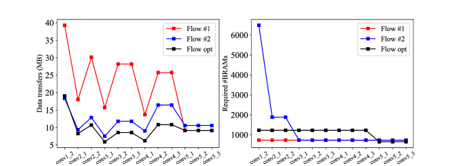
Figure 7. Complexity comparison between different dataflows

Table 1. Architecture and streaming parameter for VGG16

lyr	conv1_2	conv2_*	conv3_*	conv4_*	conv5_*
VGG16 ($K=8$, $P^{{}^{\prime}}=9$, $N^{{}^{\prime}}=64$)
$P_{s}$	243	126	108	27	9
$N_{s}$	64	128	128	512	512
VGG16 ($K=16$, $P^{{}^{\prime}}=16$, $N^{{}^{\prime}}=32$)
$P_{s}$	64	32	16	16	16
$N_{s}$	64	128	256	256	256

The required bandwidth can be easily calculated given latency budget $\tau_{i}$ in each layer $i$. We first assume the platform has enough bandwidth during computing, then $\tau_{i}$ is determined based on each layer’s computation complexity. Suppose the total latency budget for convolutional layers is $\tau$, then for each layer $\tau_{i}=\tau\times\frac{CMP_{i}}{CMP_{\text{total}}}$, where $CPM_{i}$ denotes multiplications and additions in layer $i$. Table2 gives the required bandwidth given total inference latency $\tau=20$ ms. Even with enlarged spectral kernels, the whole design still reaps significant improvements from Flow opt and avoid being communication-bounded.

Table 2. Required bandwidth for VGG16 under Flow opt

VGG16 ($K=8$, $P^{{}^{\prime}}=9$, $N^{{}^{\prime}}=64$)
lyr	conv1_2	conv2_1	conv2_2	conv3_1	conv3_2,3	conv4_1	conv4_2,3	conv5_1,2,3
BW (GB/s)	8.2	7.3	4.7	4.8	3.5	5.0	4.3	9.9

6.2. PE utilization

When evaluating the scheduling algorithm, we use PE utilization $\mu_{i}$ to show the average number active PEs in each layer $i$. Given $r$ replicas for each input image tile, since the total number of multiplications and additions are fixed, higher PE utilization means less number of processing cycles in each convolutional layer. We first define PE utilization $\mu_{i}$ in layer $i$ as:

(14) $$\mu_{i}=\frac{\sum_{t=1}^{T}PE_{\text{on}_{t}}}{T\cdot PE_{\text{total}}}=\frac{\sum_{t=1}^{T}PE_{\text{on}_{t}}}{T\cdot N^{{}^{\prime}}P^{{}^{\prime}}},$$

where $T$ denotes the total convolution cycles, each cycle contributed by Hadamard product with $P^{{}^{\prime}}$ input tiles and $N^{{}^{\prime}}$ kernels; $PE_{\text{on}_{t}}$ and $PE_{\text{total}}$ are the number of working PEs on cycle $t$, and the total number of PEs on chip.

To compare, we also implement two baseline methods: random scheduling and lowest-index first scheduling(Niu et al., 2019). random scheduling randomly chooses both a kernel and a non-zero weight index in this kernel, then continues randomly choosing other kernels and indices until either all kernels are included or the number of unique indices reaches $r$. On the other hand, lowest-index first scheduling always picks the kernels with lowest index in the current group. It iterates this operation until the same stopping condition is triggered.

Fig.8 shows PE utilization in each layer of VGG16 using above three scheduling methods with the number of replicas $r=8$, and $N^{{}^{\prime}}=64$. Exact-cover based scheduling method achieves the highest PE utilization. Moreover, it also gives a consistent performance across all convolutional layers, while lowest-index first scheduling deeply relies on the condition that indices in different kernels are close, like kernels in layer conv5_2, conv5_3.

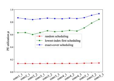
Figure 8. PE utilization given in each layer of VGG16 $r=8$

To show how PE utilization changes with the number of replicas $r$ under different scheduling methods, we vary the number of replicas $r$ from 4 to 20. Fig.9 shows the average PE utilization under different compression ratios, in which the average PE utilization is obtained by weighting each layer’s utilization with its total computations. Scheduling method in this paper reaches very high PE utilization ($>80\%$) given fewer number of replicas compared with lowest-index first method. Even under $\times 8$ compression, in which indices are largely scattered from 0 to $K^{2}-1$, exact-cover based scheduling still achieves $>80\%$ PE utilization given 10 replicas for each input tiles. Lowest-index first method, on the contrary, needs 16 replicas to reach comparable performance.

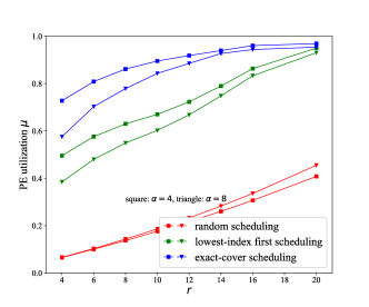
Figure 9. Average PE utilization for VGG16 given different number of replicas

Apart from sparse kernels generated by algorithm in (Niu et al., 2019), robustness to more general sparsity patterns is also critical. We generate sparse kernels from uncompressed spectral model by randomly choose $\frac{K^{2}}{\alpha}$ non-zero weights while zeroing other values. We try various compression ratios, as well as different number of replicas $r$. Fig. 10 shows the average PE utilization for these three scheduling methods. Exact-cover based methods always outperforms lowest-index first scheduling. In addition, even with random sparsity pattern, exact-cover based methods still achieves comparable PE utilization as in ADMM-based pruned kernels when $\alpha=4$.

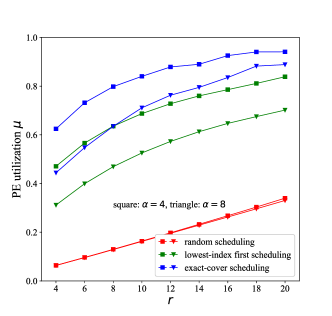
Figure 10. Average PE utilization for random non-zeros given different number of replicas

Table 3. Implementation on FPGA and comparison with other works

	(Zhang and Prasanna, 2017)	(Zeng et al., 2018)	(Niu et al., 2019)	(Page et al., 2017)	This work
Device	Intel QPI FPGA	Stratix V	Virtex XC7VX690T	Artix 7 XC7A200T	Xilinx Alveo U200
Datatype	16bit FT	16bit FX	16bit FX	16bit FX	16bit FX
DSP	224/224	256/256	3200/3600	384/740	2680/6840
BRAM	-	1377/1880	1244/1470	194/365	1469/2160
LUT	-	107K/233K	237K/430K	-	230K/1.2M
Clock(MHz)	200	200	200	100	200
Throughput(fps)	4	6	148	5	112
Latency(ms)	250	167	68	200	9
Bandwidth(GB/s)	5.0	-	9	-	12

6.3. FPGA implementation

During implementation, we choose VGG16 as our target model fed with $224\times 224$ images, in which compression ratio $\alpha=4$, corresponding accuracy is $95.0\%$. Architecture parameters $P^{{}^{\prime}},N^{{}^{\prime}}$ are set to be 9 and 64, while streaming parameters in each layer are the same as Table1. Based on the scheduling analysis, we choose the number of replicas $r$ to be 10 to get $>90\%$ PE utilization. We use the state-of-the-art FPGA, Xilinx Alveo U200, as our target platform, which has $6840$ DSPs and $2160$ RBAMs. URAM (288Kb each) is introduced recently as a global on-chip memory, which we didn’t consider in our analysis. However, our dataflow analysis can be still generalized to this new memory, for which we can translate off-chip data transfers as communication between global buffers and local buffers. Table3 shows the implementation result of our whole architecture, as well as performance comparison with other works. With using $40\%$ DSPs and $68\%$ BRAMs, we still achieve 200MHz clock frequency. Given $N^{{}^{\prime}}=64$ and $P^{{}^{\prime}}=9$, the inference in all convolutional layers is done within $9$ ms, while the required bandwidth is lowered to $12$ GB/s. (Zhang and Prasanna, 2017) and (Zeng et al., 2018) are aimed to accelerate uncompressed spectral CNNs on FPGAs. In terms of latency, we reduce the inference time by $46\%$ after simply scaling the resources utilization. Compared with (Niu et al., 2019), though it has higher throughput, it can only process images in batches. Single-image inference latency is 68ms, which is $7.5\times$ higher than the design in this paper. If we scale its latency to 9ms, the required bandwidth explodes to almost 70GB/s, which is far beyond single DDR’s capacity. (Page et al., 2017) is a design for sparse spatial CNNs. Since it uses an old device, to give a fair comparison, we also assume it can be deployed in Alveo U200, while accessing the same resources. Under 200MHz, we can still get near $40\%$ latency improvement.

To intuitively show resource utilization in the FPGA device, we give a FPGA footprint after implementation, as shown in Fig. 11. Our design take up almost $70\%$ of the total area and most routing resources, which explains why we don’t further increase BRAM and DSP usage.

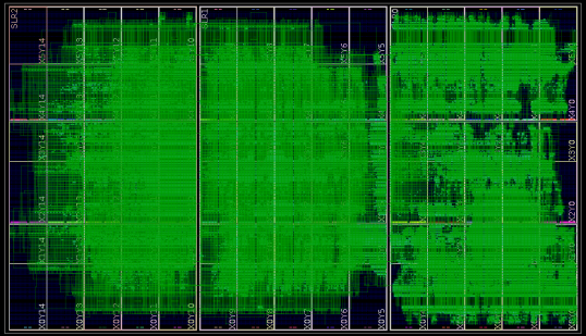
Figure 11. FPGA footprint of our design

7. Conclusion

Pruned spectral CNNs can reduce computation complexity without accuracy loss but have a kernel storage explosion problem. We develop a principled design approach to fully exploit the potential of sparse spectral CNNs and overcome the performance gap between pruning and FPGA implementation: first, we analyze the bandwidth-storage tradeoff of sparse convolutional layers and locate bottlenecks. We then adopt a flexible dataflow for different layers to minimize communication overhead. To ameliorate the performance degradation brought on by irregular on-chip memory accesses of sparse kernels, we design an approximate exact-cover based scheduling algorithm to efficiently feed PEs with few replicas. Finally, we implement a unified hardware architecture which can adjust flexible dataflow on the fly and maximize PE utilization. On a Xilinx Alveo U200 platform, with 64 parallel kernels and 9 parallel input tiles, inference takes 9ms, while only requiring 12GB/s off-chip bandwidth.

8. Acknowledgements

This work was supported in part by the National Science Foundation under grants CNS-1643351 and CCF-1919117.

References

- (1)
- Amos et al. (2016) Brandon Amos, Bartosz Ludwiczuk, Mahadev Satyanarayanan, et al. 2016. Openface: A general-purpose face recognition library with mobile applications. CMU School of Computer Science 6 (2016).
- Boyd et al. (2011) Stephen Boyd, Neal Parikh, Eric Chu, Borja Peleato, and Jonathan Eckstein. 2011. Distributed Optimization and Statistical Learning via the Alternating Direction Method of Multipliers. Found. Trends Mach. Learn. 3, 1 (Jan. 2011), 1–122. https://doi.org/10.1561/2200000016
- Chen et al. (2017) Zhuo Chen, Wenlu Hu, Junjue Wang, Siyan Zhao, Brandon Amos, Guanhang Wu, Kiryong Ha, Khalid Elgazzar, Padmanabhan Pillai, Roberta Klatzky, et al. 2017. An empirical study of latency in an emerging class of edge computing applications for wearable cognitive assistance. In Proceedings of the Second ACM/IEEE Symposium on Edge Computing. ACM, 14.
- Choquette et al. (2018) Jack Choquette, Olivier Giroux, and Denis Foley. 2018. Volta: Performance and programmability. IEEE Micro 38, 2 (2018), 42–52.
- Courbariaux et al. (2015) Matthieu Courbariaux, Yoshua Bengio, and Jean-Pierre David. 2015. Binaryconnect: Training deep neural networks with binary weights during propagations. In Advances in neural information processing systems. 3123–3131.
- Gupta et al. (2015) Suyog Gupta, Ankur Agrawal, Kailash Gopalakrishnan, and Pritish Narayanan. 2015. Deep learning with limited numerical precision. In International Conference on Machine Learning. 1737–1746.
- Han et al. (2015) Song Han, Huizi Mao, and William J Dally. 2015. Deep compression: Compressing deep neural networks with pruning, trained quantization and huffman coding. arXiv preprint arXiv:1510.00149 (2015).
- He et al. (2016) Kaiming He, Xiangyu Zhang, Shaoqing Ren, and Jian Sun. 2016. Deep residual learning for image recognition. In Proceedings of the IEEE conference on computer vision and pattern recognition. 770–778.
- He et al. (2017) Yihui He, Xiangyu Zhang, and Jian Sun. 2017. Channel pruning for accelerating very deep neural networks. In Proceedings of the IEEE International Conference on Computer Vision. 1389–1397.
- Jacob et al. (2018) Benoit Jacob, Skirmantas Kligys, Bo Chen, Menglong Zhu, Matthew Tang, Andrew Howard, Hartwig Adam, and Dmitry Kalenichenko. 2018. Quantization and training of neural networks for efficient integer-arithmetic-only inference. In Proceedings of the IEEE Conference on Computer Vision and Pattern Recognition. 2704–2713.
- Krizhevsky et al. (2012) Alex Krizhevsky, Ilya Sutskever, and Geoffrey E Hinton. 2012. Imagenet classification with deep convolutional neural networks. In Advances in neural information processing systems. 1097–1105.
- Lin et al. (2016) Darryl Lin, Sachin Talathi, and Sreekanth Annapureddy. 2016. Fixed point quantization of deep convolutional networks. In International Conference on Machine Learning. 2849–2858.
- Long et al. (2015) Jonathan Long, Evan Shelhamer, and Trevor Darrell. 2015. Fully convolutional networks for semantic segmentation. In Proceedings of the IEEE conference on computer vision and pattern recognition. 3431–3440.
- Luo et al. (2017) Jian-Hao Luo, Jianxin Wu, and Weiyao Lin. 2017. ThiNet: A Filter Level Pruning Method for Deep Neural Network Compression. In The IEEE International Conference on Computer Vision (ICCV).
- Mei et al. (2017) Chunsheng Mei, Zhenyu Liu, Yue Niu, Xiangyang Ji, Wei Zhou, and Dongsheng Wang. 2017. A 200mhz 202.4 gflops@ 10.8 w vgg16 accelerator in xilinx vx690t. In 2017 IEEE Global Conference on Signal and Information Processing (GlobalSIP). IEEE, 784–788.
- Niu et al. (2019) Yue Niu, Hanqing Zeng, Ajitesh Srivastava, Kartik Lakhotia, Rajgopal Kannan, Yanzhi Wang, and Viktor Prasanna. 2019. SPEC2: SPECtral SParsE CNN Accelerator on FPGAs. In Proceedings of the 2019 IEEE International Conference on High Performance Computing, Data, and Analytics. IEEE.
- Page et al. (2017) Adam Page, Ali Jafari, Colin Shea, and Tinoosh Mohsenin. 2017. Sparcnet: A hardware accelerator for efficient deployment of sparse convolutional networks. ACM Journal on Emerging Technologies in Computing Systems (JETC) (2017).
- Qiu et al. (2016) Jiantao Qiu, Jie Wang, Song Yao, Kaiyuan Guo, Boxun Li, Erjin Zhou, Jincheng Yu, Tianqi Tang, Ningyi Xu, Sen Song, et al. 2016. Going deeper with embedded fpga platform for convolutional neural network. In Proceedings of the 2016 ACM/SIGDA International Symposium on Field-Programmable Gate Arrays. ACM, 26–35.
- Ren et al. (2015) Shaoqing Ren, Kaiming He, Ross Girshick, and Jian Sun. 2015. Faster r-cnn: Towards real-time object detection with region proposal networks. In Advances in neural information processing systems. 91–99.
- Simonyan and Zisserman (2014) Karen Simonyan and Andrew Zisserman. 2014. Very deep convolutional networks for large-scale image recognition. arXiv preprint arXiv:1409.1556 (2014).
- Sodani et al. (2016) Avinash Sodani, Roger Gramunt, Jesus Corbal, Ho-Seop Kim, Krishna Vinod, Sundaram Chinthamani, Steven Hutsell, Rajat Agarwal, and Yen-Chen Liu. 2016. Knights landing: Second-generation intel xeon phi product. Ieee micro 36, 2 (2016), 34–46.
- Szegedy et al. (2015) Christian Szegedy, Wei Liu, Yangqing Jia, Pierre Sermanet, Scott Reed, Dragomir Anguelov, Dumitru Erhan, Vincent Vanhoucke, and Andrew Rabinovich. 2015. Going deeper with convolutions. In Proceedings of the IEEE conference on computer vision and pattern recognition. 1–9.
- Wei et al. (2017) Xuechao Wei, Cody Hao Yu, Peng Zhang, Youxiang Chen, Yuxin Wang, Han Hu, Yun Liang, and Jason Cong. 2017. Automated systolic array architecture synthesis for high throughput CNN inference on FPGAs. In Proceedings of the 54th Annual Design Automation Conference 2017. ACM, 29.
- Yaqoob et al. (2019) Ibrar Yaqoob, Latif U Khan, SM Ahsan Kazmi, Muhammad Imran, Nadra Guizani, and Choong Seon Hong. 2019. Autonomous Driving Cars in Smart Cities: Recent Advances, Requirements, and Challenges. IEEE Network (2019).
- Zeiler and Fergus (2014) Matthew D Zeiler and Rob Fergus. 2014. Visualizing and understanding convolutional networks. In European conference on computer vision. Springer, 818–833.
- Zeng et al. (2018) Hanqing Zeng, Ren Chen, Chi Zhang, and Viktor Prasanna. 2018. A framework for generating high throughput CNN implementations on FPGAs. In Proceedings of the 2018 ACM/SIGDA International Symposium on Field-Programmable Gate Arrays. ACM, 117–126.