Provable Probabilistic Imaging using Score-based Generative Priors

Abstract

Estimating high-quality images while also quantifying their uncertainty are two desired features in an image reconstruction algorithm for solving ill-posed inverse problems. In this paper, we propose plug-and-play Monte Carlo (PMC) as a principled framework for characterizing the space of possible solutions to a general inverse problem. PMC is able to incorporate expressive score-based generative priors for high-quality image reconstruction while also performing uncertainty quantification via posterior sampling. In particular, we introduce two PMC algorithms which can be viewed as the sampling analogues of the traditional plug-and-play priors (PnP) and regularization by denoising (RED) algorithms. We also establish a theoretical analysis for characterizing the convergence of the PMC algorithms. Our analysis provides non-asymptotic stationarity guarantees for both algorithms, even in the presence of non-log-concave likelihoods and imperfect score networks. We demonstrate the performance of the PMC algorithms on multiple representative inverse problems with both linear and nonlinear forward models. Experimental results show that PMC significantly improves reconstruction quality and enables high-fidelity uncertainty quantification.

1 Introduction

The problem of accurately reconstructing high-quality images $\xbm\in\R^{n}$ from a set of sparse and noisy measurements $\ybm\in\R^{m}$ is fundamental in computational imaging. These measurements often do not contain sufficient information to losslessly specify the target image, making the inverse problem ill-posed. Image reconstruction methods should account for ill-posedness in two ways: by 1) imposing prior knowledge to regularize the final solution image, and by 2) characterizing the posterior probability distribution of all possible solutions. While much of the computational imaging research has centered on exploiting prior knowledge, it remains essential to characterize the full distribution of solutions to understand uncertainty, regardless of any imposed constraints. Traditionally, either the posterior distribution is ignored or it is derived under simplified image priors to make the problem tractable, leading to biased results. The objective of this work is to leverage recent advances in learning-based generative models in order to provably specify the posterior distribution under expressive image priors.

The Bayesian framework is commonly used to infer the posterior distribution $\pi(\xbm|\ybm)$ from the prior distribution $p(\xbm)$ of the desired image by incorporating the likelihood $\ell(\ybm|\xbm)$

$$\pi(\xbm|\ybm)\propto\ell(\ybm|\xbm)p(\xbm).$$ (1)

Here, $\ell(\ybm|\xbm)$ probabilistically relates the image to the measurements and is defined by the known imaging system. The quality of the inference of $\xbm|\ybm$ directly depends on the expressivity of the prior. Classic choices include the sparsity-promoting priors such as total variation (TV) [1, 2]. However, these hand-crafted priors are not expressive enough to characterize complicated image structures. The focus has recently shifted to exploring learning-based priors due to their strong expressive power; such priors are often parameterized by deep neural networks. Plug-and-play priors (PnP) [3] and regularization by denoising (RED) [4] are two popular methods in this direction. They consider a pre-trained denoiser as an implicit image prior and use it to replace the functional prior module in the traditional iterative algorithms. Despite the practical success under deep denoisers [5, 6, 7], PnP/RED methods are essentially based on the maximum a posteriori (MAP) estimation which only produces a single image and cannot account for the full posterior distribution.

Sampling from the posterior distribution offers a principled approach to gain insight into the uncertainty and credibility of a reconstructed image. Such uncertainty quantification (UQ) is especially crucial in non-convex inverse problems where multiple distinct solutions could exist and lead to very different interpretations. Due to the complexity of image distributions, traditional UQ methods rely on simplified image assumptions that often yield limited performance [8, 9]. Recently, score-based generative models (SGM) have emerged as a powerful deep learning (DL) tool for sampling from complex high-dimensional distributions. In particular, SGMs learn the score of an image distribution and use it in a Monte Carlo Markov Chain (MCMC) algorithm to perform iterative sampling. It has been shown that SGMs achieve state-of-the-art performance in unconditional image generation [10]. Nevertheless, leveraging a SGM to conduct provable posterior sampling subject to sophisticated physical constraints is underexplored.

In this paper, we aim to bridge this gap by proposing plug-and-play Monte Carlo (PMC) as a principled posterior sampling framework for solving inverse problems. PMC is built on the fusion of PnP/RED and SGM: it leverages powerful score-based generative priors in a plug-and-play fashion, similar to PnP/RED, while enabling provable posterior sampling by incorporating the MCMC formulation used in the SGM. Specifically, the key contributions of this work are as follows:

• We demonstrate how PnP and RED can be generalized to sampling by studying their continuous limits. We show that PnP and RED converge to the same gradient-flow ordinary differential equation (ODE) of the posterior, which corresponds to the noise-free version of the Langevin stochastic differential equation (SDE). Note that this observation also leads to new insights about the mathematical equivalence between PnP and RED.

• We develop two PMC algorithms by extending PnP and RED to MCMC formulations. We name our algorithms PMC-PnP and PMC-RED, respectively. To the best of our knowledge, PMC-PnP represents a new addition to the existing sampling algorithms, while PMC-RED aligns with the common Langevin MCMC algorithm. Inspired by recent advances in SGM, we employ weighted annealing for PMC algorithms and demonstrate how it mitigates mode collapse while also accelerating the sampling speed.

• We establish a stationary-distribution convergence analysis for the proposed PMC algorithms. We prove that all PMC algorithms will converge to the posterior distribution in terms of Fisher information under potentially non-log-concave likelihoods and imperfect prior scores. Note that our analysis can be interpreted as a sampling analogue to the fixed-point analysis established for PnP/RED.

• We validate our algorithms on three real-world imaging inverse problems: compressed sensing, magnetic resonance imaging, and black-hole interferometric imaging. Here, the black-hole imaging problem corresponds to a non-log-concave likelihood. Our experimental results demonstrate improved reconstruction quality and reliable UQ enabled by the proposed PMC algorithms.

2 Background

2.1 Solving inverse problems with Bayesian inference

Consider the general inverse problem

$$\ybm=\Abm(\xbm)+\ebm,$$ (2)

where the goal is to recover $\xbm\in\R^{n}$ given the measurements $\ybm\in\R^{m}$. Here, the measurement operator $\Abm:\R^{n}\rightarrow\R^{m}$ models the response of the imaging system, and $\ebm\in\R^{m}$ represents the measurement noise, which is often assumed to be additive white Gaussian noise (AWGN). One popular Bayesian inference framework for imaging inverse problems is based on the MAP estimation:

$$\xbmhat=\argmax_{\xbm\in\R^{n}}\ell(\ybm|\xbm)p(\xbm)=\argmin_{\xbm\in\R^{n}}\big{\{}g(\xbm)+h(\xbm)\big{\}}.$$ (3)

Here, $g(\xbm)=-\log\ell(\ybm|\xbm)$ is often known as the data-fidelity term and $h(\xbm)=-\log p(\xbm)$ as the regularizer. Commonly, the data-fidelity is set to the least-square loss $g(\xbm)=\frac{1}{2\beta^{2}}\|\ybm-\Abm(\xbm)\|_{2}^{2}$, which corresponds to the Gaussian likelihood $\ybm|\xbm\sim\Ncal(\Abf(\xbm),\beta^{2}I)$ with $\beta^{2}>0$ controlling the variance.

Many popular regularizers, including those based on sparsity, are not differentiable. This precludes using simple algorithms such as gradient descent to solve (3). Proximal methods [11, 12] are commonly employed to accommodate nonsmooth regularizers by leveraging a mathematical concept known as the proximal operator

$$\prox_{\mu h}(\zbm)\defn\argmin_{\xbm\in\R^{n}}\left\{\frac{1}{2}\|\xbm-\zbm\|_{2}^{2}+\mu h(\xbm)\right\}.$$ (4)

Here, the squared error enforces the output $\xbm$ to be close to the input $\zbm$, while $h$ penalizes the solutions falling outside the constraint set with $\mu>0$ adjusting the strength. For many regularizers, the sub-optimization in (4) can be efficiently solved without differentiating $h$ [12, 2]. One commonly used proximal method is the proximal gradient method, which pairs the proximal operator with gradient descent

$${\xbm_{k+1}} =\prox_{\gamma h}\big{(}{\xbm_{k}}-\gamma\nabla g({\xbm_{k}})\big{)},$$ (5)

where $\mu$ is usually set to $\gamma$ for ensuring convergence. Note that the prior information is only imposed via $\prox_{\gamma h}$. An important insight to note is that, since the squared loss is analogous to the Gaussian likelihood in denoising problems involving AWGN, the proximal operator can be viewed as a regularized solution of an image denoising problem [2].

2.2 Using denoisers to impose image priors

Inspired by the equivalence between the proximal operator and image denoiser, PnP [3] was proposed as a pioneering method for incorporating denoising priors. The key idea of PnP is to replace the proximal operator in (4) with an arbitrary AWGN denoiser $\Dcal_{\sigma}:\R^{n}\rightarrow\R^{n}$ with $\sigma>0$ controlling the denoising strength. For example, the formulation of PnP proximal gradient method [13] is given by

$${\xbm_{k+1}} =\Dcal_{\sigma}\big{(}{\xbm_{k}}-\gamma\nabla g({\xbm_{k}})\big{)}$$ (6)

where $\gamma>0$ denotes the step-size. However, the denoiser may not correspond to any explicit regularizer $h$, making PnP generally lose the interpretation as proximal optimization. Other PnP algorithms have also been proposed based on different formulations [14, 15, 16], and we refer to [17] for a comprehensive review.

RED [4] is an alternative method for leveraging image denoiser within MAP optimization algorithms. Different from PnP, RED does not rely on the proximal-denoiser connection but uses the noise residual to approximate the gradient of an implicit regularizer. One widely-used example is the RED gradient descent [4]

$${\xbm_{k+1}}={\xbm_{k}}-\gamma\Big{(}\nabla g({\xbm_{k}})+\tau\big{(}{\xbm_{k}}-\Dcal_{\sigma}({\xbm_{k}})\big{)}\Big{)}$$ (7)

where $\tau>0$ is the regularization parameter. In some special cases, RED is able to link the noise residual $\xbm-\Dcal_{\sigma}(\xbm)$ to an explicit regularizer $h(\xbm)=\xbm^{\Tsf}(\xbm-\Dcal_{\sigma}(\xbm))$ [4, 18]; however, such RED regularizer do not exist for general denoisers, including those parameterized by deep neural networks.

Table 1: A conceptual comparison of existing posterior sampling methods for probabilistic imaging

Category	Reference	2cmGenerative prior	2cmModel agnostic	2cmType of $A(\cdot)$	2cmTheoretical guarantee
2cmVariational Bayesian	[19]	✗	✗	General	✗
	[20]	✓	✗	General	✗
2cmDM-based	[21]	✓	✓	Linear	✗
	[22]	✓	✓	General	✗
	[23]	✓	✗	Linear	✗
2cmMCMC-based	[24]	✓	✓	Linear	✓✗${}^{1}$
	[25]	✓	✓	Linear	✗
	[26]	✗	✓	Linear${}^{2}$	✓✗${}^{3}$
	[27]	✓	✓	Linear	✗
	[28]	✗	✓	Linear	✓✗${}^{4}$
2cmMCMC-based	Ours	✓	✓	General	✓

${}^{1}$Only applicable to Gaussian $\Abm(\cdot)$. ${}^{3}$Not applicable to annealing.

${}^{2}$Theoretically applicable to general $\Abm(\cdot)$ ${}^{4}$No convergence rate presented.

under other assumptions.

The success of PnP and RED has motivated theoretical studies to understand their convergence under general denoisers. Due to the nonexistence of explicit regularizers, PnP and RED are commonly interpreted as fixed-point iterations, and their convergence to a fixed point has been shown for various algorithms [14, 29, 30, 31, 16, 32, 33, 34, 35, 36, 37, 38, 39]. There has also been considerable interest in studying the mathematical equivalence between PnP and RED. Analysis has been proposed to connect RED with the Moreau envelope [36, 40], which allows RED to be interpreted as a generalization of proximal optimization. Nevertheless, a direct algorithmic equivalence between (6) and (7) is still absent in the literature.

2.3 Score-based generative models (SGM)

SGMs have been recently proposed as a powerful generative method for drawing samples from a complex high-dimensional distribution. The main idea of SGMs is to use the score $\nabla\log p(\xbm)$ of the desired distribution $p$ in either MCMC algorithms [41] or diffusion models (DM) [42, 43].

As the true score is almost impossible to obtain for complex distributions $p$, a SGM resorts to finding a computable approximation of $\nabla\log p$ in the form of a neural network. One elegant approximation is inspired by Tweedie’s formula [44]. Let $\zbm\sim p$ be a random sample from the desired distribution, $\ebm\sim\Ncal(0,\sigma^{2}I)$ the AWGN, and $\xbm=\zbm+\ebm$ the noisy image. Then, we have

$$\nabla\log p_{\sigma}(\xbm)=\frac{\E[\zbm|\xbm]-\xbm}{\sigma^{2}}$$ (8)

where $\E[\zbm|\xbm]$ is the minimum mean squared error (MMSE) estimator of $\zbm$ given $\xbm$, and $p_{\sigma}$ is the distribution of the noisy image, which is distinct from the distribution of $p$ itself. As the sum of random variables results in a distribution equal to the convolution of their individual distributions, $p_{\sigma}$ is given by p_σ() = ∫_^n p() ϕ_σ(-)d, where $\phi_{\sigma}$ denotes the probability density function of $\Ncal(0,\sigma^{2}I)$. The distribution $p_{\sigma}$ can be intuitively interpreted as a smoothed version of the true distribution. Given that the Gaussian distribution is a type of mollifier, we can show $\nabla\log p_{\sigma}\rightarrow\nabla\log p$ as $\sigma\rightarrow 0$. An extension of (8) leads to the denoising score matching (DSM) loss [45] that enables learning the score of the smoothed prior from data

$$\textsf{DSM}(\theta)=\E\left[\left\|\frac{\zbm-\xbm}{\sigma^{2}}-\Scal_{\theta}(\xbm,\sigma)\right\|_{2}^{2}\right]$$ (9)

where $\Scal_{\theta}(\xbm,\sigma)$ is a score network parameterized by $\theta$ that is meant to approximate $\nabla\log p_{\sigma}(\xbm)$. For a review of recent SGM algorithms, we refer to the survey presented in [10].

2.4 Related probabilistic imaging methods

We here review the related methods that leverage DL models to perform posterior sampling defined in (1). Table 2.2 provides a conceptual comparison of the methods discussed in this section.

2.4.1 Variational Bayesian methods

Deep variational Bayesian methods often parameterize the posterior distribution as a deep neural network, which can be trained by minimizing the evidence lower bound (ELBO). It has been shown that ELBO is related to the Kullback-Leibler divergence with respect to (w.r.t.) the posterior distribution [46]. Recent works have leveraged this methodology for probabilistic imaging under either hand-crafted [19] or score-based priors [20]. However, the evaluation of the ELBO requires access to the log prior. Due to this requirement, [20] needs to solve an expensive high-dimensional ODE to obtain the log prior associated with the score network, making itself unscalable to large-scale imaging problems. A follow-up work [47] addresses the computation limit at the cost of using an inexact log prior.

2.4.2 DM-based methods

A DM is one type of SGM that learns to sample a distribution $p$ by reversing a diffusion process from $p$ to some simple distribution [10]. The two processes can be mathematically formulated as a diffusion SDE and its reverse-time SDE that relies on the time-varying score $\nabla\log p_{t}(\xbm_{t})$. To adapt DMs for posterior sampling, recent works focus on constraining the reverse process by integrating the likelihood. One line of work uses the proximal operator [21, 23], while others resort to leveraging the gradient [22]. Unfortunately, these methods generally lack theoretical guarantees on their convergence to the posterior distribution. Recent experimental evidence [20, 48] shows that they lead to inaccurate sampling even in simple cases.

2.4.3 MCMC-based methods

MCMC methods recently received significant interest due to the emergence of SGMs. The majority of MCMC-based methods for imaging inverse problems are based on the Langevin MCMC. Recent works have studied the incorporation of linear forward models via singular value decomposition (SVD) [25] or the recovery analysis under random Gaussian matrix [24]. However, these works lack theoretical guarantees on their convergence to the posterior distribution. A recent work [26] analyzed the convergence of Langevin MCMC for posterior sampling under strong assumptions of the forward model. Our work significantly differs from [26] by establishing a novel convergence analysis that relies on weaker assumptions and is compatible with weighted annealing. Other MCMC algorithm has also been investigated for posterior sampling. A line of concurrent works combines the Gibbs splitting with either denoising [28] or generative priors [27].

Algorithm 1 Plug-and-play Monte Carlo (PMC)

1: input: $\xbm_{0}\in\R^{n}$, $\gamma>0$, and $\sigma>0$.

2: for $k=0,1,\dots,N-1$ do

3:    ${\Zbm_{k}}\leftarrow\Ncal(0,I)$

4:    switch discretization

5:     case PnP: (PMC-PnP)

6:      $\Pcal({\xbm_{k}})\leftarrow\nabla g({\xbm_{k}})-\Scal_{\theta}\big{(}{\xbm_{k}}-\gamma\nabla g({\xbm_{k}}),\sigma\big{)}$

7:      ${\xbm_{k+1}}\leftarrow{\xbm_{k}}-\gamma\Pcal({\xbm_{k}})+\sqrt{2\gamma}{\Zbm_{k}}$

8:     case RED: (PMC-RED)

9:      $\Gcal({\xbm_{k}})\leftarrow\nabla g({\xbm_{k}})-\Scal_{\theta}\big{(}{\xbm_{k}},\sigma\big{)}$

10:      ${\xbm_{k+1}}\leftarrow{\xbm_{k}}-\gamma\Gcal({\xbm_{k}})+\sqrt{2\gamma}{\Zbm_{k}}$

11: end for

3 Method: Plug-and-Play Monte Carlo

We start the presentation of PMC by deriving the gradient-flow ODE as the continuous limit of both PnP and RED. By extending the gradient-flow ODE to Langevin SDE, we then formulate the PMC algorithms. Lastly, we present the annealed PMC algorithms by introducing weighted annealing.

3.1 Continuous-time interpretation of PnP/RED

Let $\Rcal_{\sigma}\defn Id-\Dcal_{\sigma}$ be the residual predictor. Consider the following reformulation of the PnP algorithm in (6)

$${\xbm_{k+1}} =\Dcal_{\sigma}\big{(}{\xbm_{k}}-\gamma\nabla g({\xbm_{k}})\big{)}$$

$$={\xbm_{k}}-\gamma\Big{(}\nabla g({\xbm_{k}})+\frac{1}{\gamma}\Rcal_{\sigma}\big{(}{\xbm_{k}}-\gamma\nabla g({\xbm_{k}})\big{)}\Big{)},$$ (10)

and the RED algorithm in (7)

$${\xbm_{k+1}} ={\xbm_{k}}-\gamma\Big{(}\nabla g({\xbm_{k}})+\tau\big{(}\xbm-\Dcal_{\sigma}(\xbm)\big{)}\Big{)}$$

$$={\xbm_{k}}-\gamma\Big{(}\nabla g({\xbm_{k}})+\tau\Rcal_{\sigma}\big{(}{\xbm_{k}}\big{)}\Big{)}.$$ (11)

If $\Dcal_{\sigma}(\xbm)$ is an MMSE image denoiser, by invoking Tweedie’s formula in (8) we can derive the residual predictor as $\Rcal(\xbm)=-\sigma^{2}\nabla\log p_{\sigma}(\xbm)$. Plugging the residual predictor into (3.1) and (3.1) and rearranging the terms yields the following discrete gradient-flow formulation for PnP

$$\frac{{\xbm_{k+1}}-{\xbm_{k}}}{\gamma}=-\Pbf({\xbm_{k}})\quad\text{where}$$

$$\Pbf(\xbm)\defni\nabla g(\xbm)-(\sigma^{2}/\gamma)\nabla\log p_{\sigma}\big{(}\xbm-\gamma\nabla g(\xbm)\big{)}$$ (12)

and for RED

$$\frac{{\xbm_{k+1}}-{\xbm_{k}}}{\gamma}=-\Gbf({\xbm_{k}})\quad\text{where}$$

$$\Gbf(\xbm)\defni\nabla g(\xbm)-\tau\sigma^{2}\nabla\log p_{\sigma}(\xbm).\quad\quad\quad\quad\quad\;$$ (13)

Note that the dynamics of PnP and RED are fully characterized by $\Pbf(\xbm)$ and $\Gbf(\xbm)$, respectively. Let $\tau=1/\gamma$ and $\lim_{\gamma\rightarrow 0}\{\sigma^{2}/\gamma\}=1$. We have

$$\lim_{\gamma\rightarrow 0}\Pbf(\xbm) =\nabla g(\xbm)-\lim_{\gamma\rightarrow 0}\big{\{}(\sigma^{2}/\gamma)\nabla\log p_{\sigma}\big{(}\xbm-\gamma\nabla g({\xbm_{k}})\big{)}\big{\}}$$

$$=\nabla g(\xbm)-\lim_{\gamma\rightarrow 0}\big{\{}\tau\sigma^{2}\nabla\log p_{\sigma}\vphantom{\big{(}\big{)}}(\xbm)\big{\}}=\lim_{\gamma\rightarrow 0}\Gbf(\xbm)$$

$$=-\nabla\log\ell(\ybm|\xbm)-\nabla\log p(\xbm)$$

$$=-\nabla\log\pi(\xbm|\ybm),$$ (14)

where we assume $\nabla\log p(\xbm)$ to be a continuous function. Note that $\lim_{\gamma\rightarrow 0}\{\sigma^{2}/\gamma\}=1$ ensures that $\sigma$ decays with smaller $\gamma$, resembling the requirement in proximal gradient method that the strength of the proximal operator $\mu$ is set to $\gamma$. By plugging the limits of $\Pbf(\xbm)$ and $\Gbf(\xbm)$ into (3.1) and (3.1) and taking $\gamma$ to zero, it follows that PnP and RED both converge to the gradient-flow ODE given by

$${d\xbm_{t}}=\nabla\log\pi({\xbm_{t}}|\ybm)dt.$$ (15)

With this continuous picture, we can draw a few insights about PnP and RED that are not clear through the discrete formulations. First, both PnP and RED are governed by the exact same gradient-flow ODE under the MMSE denoiser. Although the two algorithms apply the residual predictor to different iterates, they can be viewed as simply using different discretization strategies for numerically computing the ODE. Second, the gradient-flow ODE links PnP/RED to the Langevin diffusion described by the following SDE

$${d\xbm_{t}}=\nabla\log\pi({\xbm_{t}}|\ybm)dt+\sqrt{2}{d\Bbm_{t}},$$ (16)

where $\{{\Bbm_{t}}\}_{t\geq 0}$ denotes the $n$-dimensional Brownian motion. As shown in the seminal work [49], Langevin diffusion can be interpreted as the gradient flow in the space of probability distributions. The symmetry between (15) and (16) inspires us to develop the parallel MCMC algorithms of PnP/RED for posterior sampling.

3.2 Formulation of PMC-PnP/RED

The derivation of PMC-PnP and PMC-RED is based on discretizing the Langevin diffusion in (16) according to the discretization strategies used in PnP and RED, respectively. To approximate $\nabla\log p_{\sigma}(\xbm)$, one can use an MMSE image denoiser $\Dcal_{\sigma}(\xbm)=\E[\zbm|\xbm]$ as in PnP/RED; however, it is difficult to obtain an exact MMSE denoiser in practice. As the score is the key, we instead bypass this difficulty by leveraging a score network to obtain a direct approximation $\Scal_{\theta}(\xbm,\sigma)\approx\nabla\log p_{\sigma}(\xbm)$. The formulation of PMC-PnP is given by following (3.1) and (16)

$${\xbm_{k+1}}={\xbm_{k}}-\gamma\Pcal({\xbm_{k}})+\sqrt{2\gamma}{\Zbm_{k}}$$

$$\text{where}\quad\Pcal(\xbm)=\nabla g(\xbm)-\Scal_{\theta}\big{(}\xbm-\gamma\nabla g(\xbm),\sigma\big{)},$$ (17)

where ${\Zbm_{k}}=\int_{k}^{k+1}{d\Bbm_{t}}$ follows the $n$-dimensional i.i.d normal distribution. The coefficient $\sigma^{2}/\gamma$ is omitted as it does not affect the convergence of (3.2) to (16) when $\gamma\rightarrow 0$ and $\sigma\rightarrow 0$. Similarly, we can derive PMC-RED

$${\xbm_{k+1}}={\xbm_{k}}-\gamma\Gcal({\xbm_{k}})+\sqrt{2\gamma}{\Zbm_{k}}$$

$$\text{where}\quad\Gcal(\xbm)=\nabla g(\xbm)-\Scal_{\theta}(\xbm,\sigma),\quad\quad\quad\quad\;$$ (18)

where $\tau$ is also omitted. Algorithms 1 summarizes the details of PMC-PnP and PMC-RED. When $\sigma$ is sufficiently small, PMC-PnP/RED approximately samples from the true posterior distribution. In section 4, we present a detailed analysis of both PMC algorithms. We note that PMC-RED resembles the plug-and-play unadjusted Langevin algorithm (PnP-ULA) in [26], while PMC-PnP has not been studied in the existing literature.

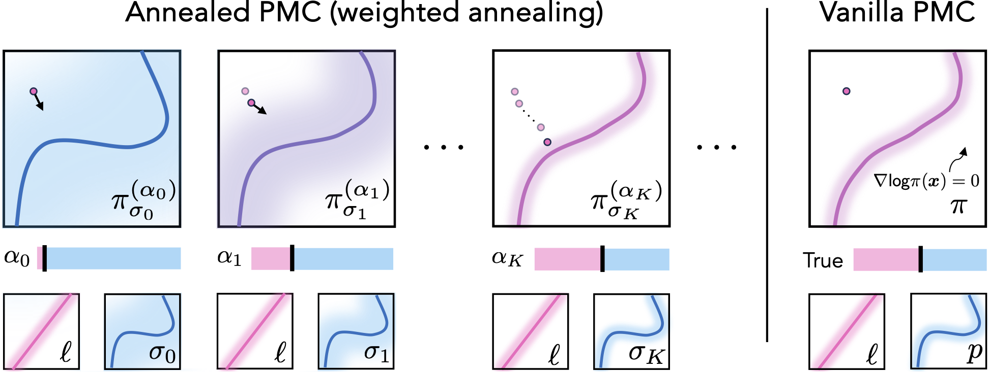
Figure 1: Conceptual illustration of how weighted annealing improves the convergence of APMC algorithms by introducing the weighted posteriors $\{\pi^{({\alpha_{k}})}_{\sigma_{k}}\}$. The solid curves and shade respectively denote the mean and probability density of the distribution; the white area means $\nabla\log p(\xbm)=0$. In order to facilitate the vanilla PMC algorithm to escape from plateaus in $\nabla\log p(\xbm)$, weighted annealing progressively decreases 1) the smoothing strength (${\sigma_{k}}$) of the prior and 2) its relative weights (${\alpha_{k}}$) to the likelihood.

3.3 Weighted annealing for enhanced performance

Langevin algorithms are known to suffer from slow convergence and mode collapse when sampling high-dimensional multimodal distributions. Inspired by the annealed importance sampling [50], we propose weighted annealing for alleviating these problems. Our strategy considers a sequence of weighted posterior distributions

$$\pi^{({\alpha_{k}})}_{\sigma_{k}}(\xbm|\ybm)\propto\ell(\ybm|\xbm)p_{\sigma_{k}}^{\alpha_{k}}(\xbm),$$

where $$\alpha_{0}>\alpha_{1}>\dots>\alpha_{K}=\dots=\alpha_{N-1}=1,$$

$$\sigma_{0}>\sigma_{1}>\dots>\sigma_{K}=\dots=\sigma_{N-1}\approx 0,$$

where $\{{\alpha_{k}}\}_{k=0}^{N-1}$ and $\{{\sigma_{k}}\}_{k=0}^{N-1}$ decays from large initial values to one and almost zero, respectively.

Note that $\alpha$ adjusts the relative weights of the likelihood and prior via powering. At the beginning, the weighted posterior is dominated by the smoothed prior $p_{\sigma_{k}}$, whose density is less concentrated and can facilitate the algorithm to escape from the plateaus in $\nabla\log p(\xbm)$. As the iteration number increases, the likelihood starts to contribute more strongly, and the smoothed prior $p_{\sigma_{k}}$ becomes similar to the true prior $p$. Fig. 1 conceptually illustrates this evolution. Intuitively, this procedure can be interpreted as a burn-in for finding a better initialization. In practice, we observe that the weighted annealing works the best when $\{\alpha\}_{k=0}^{N-1}$ and $\{\sigma\}_{k=0}^{N-1}$ shares the same schedule.

Algorithm 2 summarizes the details of the annealed PMC-PnP (APMC-PnP) and PMC-RED (APMC-RED). A powering-free strategy has been proposed in [24], which applies $\sigma$-smoothing to both likelihood and prior under heterogenous schedules. Ours differs from [24] by using a shared schedule and combining the $\alpha$-powering and $\sigma$-smoothing mechanisms. In the next section, we also analyze the convergence of the APMC algorithms.

Algorithm 2 Annealed plug-and-play Monte Carlo (APMC)

1: input: $\xbm_{0}\in\R^{n}$, $\gamma>0$, $\alpha_{0}>0$, and $\sigma_{0}>0$.

2: for $k=0,1,\dots,N-1$ do

3:    ${\Zbm_{k}}\leftarrow\Ncal(0,I)$

4:    $\sigma_{k},\alpha_{k}\leftarrow\mathsf{WeightedAnnealing}(\sigma_{0},\alpha_{0},k)$.

5:    switch discretization

6:     case PnP: (APMC-PnP)

7:      $\Pcal_{k}({\xbm_{k}})\leftarrow\nabla g({\xbm_{k}})-\alpha_{k}\Scal_{\theta}\big{(}{\xbm_{k}}-\gamma\nabla g({\xbm_{k}}),\sigma_{k}\big{)}$

8:      ${\xbm_{k+1}}\leftarrow{\xbm_{k}}-\gamma\Pcal_{k}({\xbm_{k}})+\sqrt{2\gamma}{\Zbm_{k}}$

9:     case RED: (APMC-RED)

10:      $\Gcal_{k}({\xbm_{k}})\leftarrow\nabla g({\xbm_{k}})-{\alpha_{k}}\Scal_{\theta}\big{(}{\xbm_{k}},{\sigma_{k}}\big{)}$

11:      ${\xbm_{k+1}}\leftarrow{\xbm_{k}}-\gamma\Gcal_{k}({\xbm_{k}})+\sqrt{2\gamma}{\Zbm_{k}}$

12: end for

4 Stationary-Distribution Analysis

Inspired by the fixed-point analysis of PnP/RED, we seek to establish the stationary-distribution convergence for the proposed PMC algorithms. We start our analysis by first introducing the optimization interpretation of Langevin diffusion [49]. Then, we present the assumptions and main results for the vanila and annealed PMC algorithms, respectively.

4.1 Langevin diffusion as optimization

Consider the following optimization of Kullback-Leibler (KL) divergence in the space of probability distributions equipped with the Wasserstein metric

$$\argmin_{\nu}\;\KL(\nu\,\|\,\pi)$$

$$\text{where}\quad\KL(\nu\,\|\,\pi)=\int_{\R^{n}}\nu(\xbm)\log\frac{\nu(\xbm)}{\pi(\xbm)}d\xbm.$$ (19)

where $\pi$ denotes the desired posterior distribution and $\nu$ the iterate. Similar to the gradient concept in the Euclidean space, the gradient under the Wasserstein metric can be defined [51]. In particular, the Wasserstein gradient of $\KL(\nu\,|\,\pi)$ is given by $\nabla_{\nu}\KL(\nu\,|\,\pi)=\nabla\log\frac{\nu(\xbm)}{\pi(\xbm)}$ [52], and its expected norm is known as the relative Fisher information (FI)

$$\FI(\nu\,\|\,\pi)=\int_{\R^{n}}\left\|\nabla\log\frac{\nu(\xbm)}{\pi(\xbm)}\right\|^{2}_{2}\nu(\xbm)d\xbm.$$ (20)

If ${\nu_{t}}$ denotes the distribution obtained by Langevin diffusion at time $t$, then the time derivative of $\KL({\nu_{t}}\,\|\,\pi)$ is the negative FI, i.e. $\frac{d}{dt}\KL({\nu_{t}}\,\|\,\pi)=-\FI({\nu_{t}}\,\|\,\pi)$ [52, 51], which shows that the Langevin diffusion is a gradient flow in the probability space. From an optimization point of view, $\FI(\nu_{t}\,\|\,\pi)$ is analogous to the $\ell$-2 norm of the gradient in $\R^{n}$[53]. To leverage this, we derive the convergence of $\FI(\nu_{t}\,\|\,\pi)$ under a continuous interpolation of the distributions obtained by PMC algorithms (see Supplement I for more details), which implies the stationarity of the discrete algorithms. Different from optimization, if $\nu$ and $\pi$ have positive and smooth densities, $\FI(\nu\,\|\,\pi)=0$ indicates that $\nu$ and $\pi$ are equal. This implies that the value of FI can serve as a criterion to measure the convergence of distributions. We refer to [53] for more discussion on this topic.

4.2 Convergence of stationary PMC algorithms

We begin our analysis by first considering the stationary PMC algorithms without weighted annealing. We assume that the log-likelihood $\log\ell(\ybm|\xbm)$ is differentiable and has a Lipschitz continuous gradient with constant $L_{g}>0$ for any $\xbm_{1},\xbm_{2}\in\R^{n}$

$$\big{\|}\nabla\log\ell(\ybm|\xbm_{1})-\nabla\log\ell(\ybm|\xbm_{2})\big{\|}_{2}\leq L_{g}\big{\|}\xbm_{1}-\xbm_{2}\big{\|}_{2}.$$ (A1)

This is equivalent to assuming $\nabla g(\xbm)=-\nabla\log\ell(\ybm|\xbm)$ to be Lipschitz continuous with $L_{g}$. Note that Assumption 4.2 does not assume the log-concavity of the likelihood (i.e. convexity of the data-fidelity term), meaning that our analysis is compatible with nonlinear inverse problems.

We assume that the log-prior $\log p(\xbm)$ is differentiable and has a Lipschitz continuous gradient with a finite constant $L_{p}>0$ for any $\xbm_{1},\xbm_{2}\in\R^{n}$

$$\big{\|}\nabla\log p(\xbm_{1})-\nabla\log p(\xbm_{2})\big{\|}_{2}\leq L_{p}\big{\|}\xbm_{1}-\xbm_{2}\big{\|}_{2}.$$ (A2)

This assumption is general and only poses the basic regularity condition for the underlying true prior.

We assume the score network $\Scal_{\theta}(\xbm,\sigma)$ satisfies the following conditions

1. For any $\sigma>0$, $\Scal_{\theta}(\xbm,\sigma)$ is Lipschitz continuous with $L_{\sigma}>0$ for any $\xbm_{1},\xbm_{2}\in\R^{n}$

   $$\|\Scal_{\theta}(\xbm_{1},\sigma)-\Scal_{\theta}(\xbm_{2},\sigma)\|_{2}\leq L_{\sigma}\|\xbm_{1}-\xbm_{2}\|_{2}$$ (A3.a)

2. For any $\sigma>0$, $\Scal_{\theta}(\xbm,\sigma)$ has a bounded error $\varepsilon_{\sigma}<+\infty$ for any $\xbm\in\R^{n}$

   $$\|\Scal_{\theta}(\xbm,\sigma)-\nabla\log p_{\sigma}(\xbm)\|^{2}_{2}\leq\varepsilon_{\sigma}^{2}$$ (A3.b)

We highlight that Assumption .() accounts for the network approximation error that is inevitable in practice.

Let $p_{\sigma}(\xbm)=\int_{\R^{n}}p(\zbm)\phi_{\sigma}(\xbm-\zbm)d\zbm$ denote the smoothed prior, where $\phi_{\sigma}$ is the probability density function of $\Ncal(0,\sigma^{2}I)$. We assume $\log p_{\sigma}(\xbm)$ is continuously differentiable, and $\nabla\log p_{\sigma}(\xbm)$ has a bounded error from $\nabla\log p(\xbm)$, that is, for any $\sigma>0$ and $\xbm\in\R^{n}$

$$\|\nabla\log p_{\sigma}(\xbm)-\nabla\log p(\xbm)\|_{2}\leq\sigma C.$$ (A4)

In special cases, such as $p$ being a Gaussian, the bound of the score mismatch can be derived analytically. However, it is generally difficult to derive a closed-form expression of the mismatch for an arbitrary distribution.

Under these assumptions, we now derive the convergence of PMC-RED.

Theorem 4.1 (PMC-RED).

Let $\{\nu_{t}\}_{t\geq 0}$ denote a continuous interpolation of the distributions generated by PMC-RED and $N>0$ the total number of iterations. Assume that Assumptions 4.2-4.2 hold. Then, for $\gamma\in\left(0,\frac{1}{\sqrt{32}L}\right]$, we have

$$\frac{1}{N\gamma}\int_{0}^{N\gamma}\FI(\nu_{t}\,\|\,\pi)\,dt\leq\frac{4\KL(\nu_{0}\,\|\,\pi)}{N\gamma}+\underbrace{\vphantom{\Big{|}}\Asf_{1}\gamma}_{\begin{subarray}{c}\text{Discretization}\\ \text{Error}\end{subarray}}+\underbrace{\vphantom{\Big{|}}\Asf_{2}\sigma^{2}}_{\begin{subarray}{c}\text{Score Mismatch}\\ \text{Error}\end{subarray}}+\underbrace{\vphantom{\Big{|}}\Asf_{3}\varepsilon_{\sigma}^{2}}_{\begin{subarray}{c}\text{Approximation}\\ \text{Error}\end{subarray}}$$ (T1)

where $L=L_{g}+\max\{L_{\sigma},L_{p}\}$. Note that the constants $\Asf_{1}$, $\Asf_{2}$, and $\Asf_{3}$ are independent of $\gamma$, $\sigma^{2}$, and $\varepsilon^{2}_{\sigma}$.

Proof 4.2.

See Supplement I.B for a detailed proof.

In order to derive the result for PMC-PnP we need one additional assumption on the likelihood: We assume that the $\ell$-2 norm of the gradient of log-likelihood is bounded, namely $\|\nabla g(\xbm)\|_{2}\leq R_{g}$ with $R_{g}>0$. The boundness of the $\nabla g(\xbm_{k})$ is practical and can be achieved by imposing gradient clipping at every iteration. In practice, we observe that the algorithm converges under a Gaussian likelihood without clipping.

Theorem 4.3 (PMC-PnP).

Let $\{\nu_{t}\}_{t\geq 0}$ denote a continuous interpolation of the distributions generated by PMC-PnP and $N>0$ the total number of iterations. Assume that Assumptions 4.2-4.2 hold. Then, for $\gamma\in\left(0,\frac{1}{\sqrt{32}L}\right]$, we have

$$\frac{1}{N\gamma}\int_{0}^{N\gamma}\FI(\nu_{t}\,\|\,\pi)\,dt\leq\frac{4\KL(\nu_{0}\,\|\,\pi)}{N\gamma}+\underbrace{\vphantom{\Big{|}}\Bsf_{1}\gamma}_{\begin{subarray}{c}\text{Discretization}\\ \text{Error}\end{subarray}}+\underbrace{\vphantom{\Big{|}}\Bsf_{2}\sigma^{2}}_{\begin{subarray}{c}\text{Score Mismatch}\\ \text{Error}\end{subarray}}+\underbrace{\vphantom{\Big{|}}\Bsf_{3}\varepsilon_{\sigma}^{2}}_{\begin{subarray}{c}\text{Approximation}\\ \text{Error}\end{subarray}}$$ (T2)

where $L=L_{g}+\max\{L_{\sigma}+\gamma L_{g}L_{\sigma},L_{p}\}$. Note that the constants $\Bsf_{1}$, $\Bsf_{2}$, and $\Bsf_{3}$ are independent of $\gamma$, $\sigma^{2}$, and $\varepsilon^{2}_{\sigma}$.

Proof 4.4.

See Supplement I.C for a detailed proof.

The expressions for the constants in Theorems 4.1 and 4.3 are given in the proofs. The resemblance in these two theorems shows that PMC-RED and PMC-PnP possess similar convergence behaviors. When the two algorithms run in continuous time with the true prior score (i.e. $\gamma=0$, $\sigma=0$, and $\varepsilon_{\sigma}=0$), they converge to the posterior distribution $\pi$ in terms of FI at the rate of $O(1/N)$. On the other hand, if we consider the approximations introduced in practice, their convergence is dependent on the interplay of three different errors, which are respectively proportional to step-size $\gamma$, squared smoothing strength $\sigma^{2}$, and squared approximation error $\varepsilon_{\sigma}^{2}$. While it is almost impossible to train a score network such that $\varepsilon_{\sigma}=0$, one can still adjust $\gamma$ and $\sigma$ to improve the convergence accuracy. For example, when the step-size is $O(1/N)$, the discretization error asymptotically equals zero as $N$ goes to infinity.

4.3 Convergence of annealed PMC algorithms

Characterizing the convergence of the annealed PMC algorithms is more challenging as the intermediate posterior varies over iterations. In this section, we tackle this problem by deriving explicit bounds of FI for APMC algorithms.

We assume that the output of the score network $\Scal_{\theta}(\xbm,\sigma)$ is bounded in $\ell$-2 norm, namely $\|\Scal_{\theta}(\xbm,\sigma)\|_{2}\leq R_{s}$. This assumption assumes the boundness of the deep score network’s output. Similarly, we can implement this condition in practice by using clipping.

Note that Assumption 4.2 ensures the Lipschitz constant of the true score is not exploding. This is necessary for the existence of $\sup\{L_{\sigma_{k}}\}_{k=0}^{N-1}$ as $N$ goes to infinity. Here, $L_{\sigma_{k}}$ denotes the Lipschitz constant of the score network at iteration $k$.

Theorem 4.5 (APMC-RED).

Let $\{{\alpha_{k}}\}_{k=0}^{N-1}$ and $\{{\sigma_{k}}\}_{k=0}^{N-1}$ be decreasing sequences where $\alpha_{K,\dots,N-1}=1$. Let $\{\nu_{t}\}_{t>0}$ denote a continuous interpolation of the distributions generated by APMC-RED and $N>0$ be the total number of iterations. Assume that Assumptions 4.2-4.2 and 4.3 hold. Then, for $\gamma\in\left(0,\frac{1}{\sqrt{32}L_{\mathsf{\tiny max}}}\right]$, we have

$$\frac{1}{N\gamma}\int_{0}^{N\gamma}\FI(\nu_{t}\,\|\,\pi)\,dt\leq\frac{4\KL(\nu_{0}\,\|\,\pi)+\gamma\zeta}{N\gamma}+\underbrace{\vphantom{\Big{|}}\Csf_{1}\gamma}_{\begin{subarray}{c}\text{Discretization}\\ \text{Error}\end{subarray}}+\underbrace{\vphantom{\Big{|}}\Csf_{2}\bar{\sigma}^{2}}_{\begin{subarray}{c}\text{Score Mismatch}\\ \text{Error}\end{subarray}}+\underbrace{\vphantom{\Big{|}}\Csf_{3}\bar{\varepsilon}^{2}}_{\begin{subarray}{c}\text{Approximation}\\ \text{Error}\end{subarray}}$$ (T3)

where $L_{k}=L_{g}+\max\{{\alpha_{k}}L_{\sigma_{k}},L_{p}\}$, $L_{\mathsf{\tiny max}}=\sup\,\{L_{k}\}_{k=0}^{N-1}$, $\bar{\varepsilon}^{2}=\frac{1}{N}\sum_{k=0}^{N-1}\varepsilon_{\sigma_{k}}^{2}$, and $\bar{\sigma}^{2}=\frac{1}{N}\sum_{k=0}^{N-1}\sigma^{2}_{k}$. Note that the constants $\zeta$, $\Csf_{1}$, $\Csf_{2}$, and $\Csf_{3}$ are independent of $\gamma$, $\bar{\sigma}^{2}$, and $\bar{\varepsilon}^{2}$.

Proof 4.6.

See Supplement I.D for a detailed proof.

Theorem 4.7 (APMC-PnP).

Let $\{{\alpha_{k}}\}_{k=0}^{N-1}$ and $\{{\sigma_{k}}\}_{k=0}^{N-1}$ be decreasing sequences where $\alpha_{K}=\alpha_{K+1}=\dots=1$. Let $\{\nu_{t}\}_{t>0}$ denote a continuous interpolation of the distributions generated by APMC-PnP and $N>0$ be the total number of iterations. Assume that Assumptions 4.2-4.3 hold. Then, for $\gamma\in\left(0,\frac{1}{\sqrt{32}L_{\mathsf{\tiny max}}}\right]$, we have

$$\frac{1}{N\gamma}\int_{0}^{N\gamma}\FI(\nu_{t}\,\|\,\pi)\,dt\leq\frac{4\KL(\nu_{0}\,\|\,\pi)+\gamma\zeta}{N\gamma}+\underbrace{\vphantom{\Big{|}}\Dsf_{1}\gamma}_{\begin{subarray}{c}\text{Discretization}\\ \text{Error}\end{subarray}}+\underbrace{\vphantom{\Big{|}}\Dsf_{2}\bar{\sigma}^{2}}_{\begin{subarray}{c}\text{Score Mismatch}\\ \text{Error}\end{subarray}}+\underbrace{\vphantom{\Big{|}}\Dsf_{2}\bar{\varepsilon}^{2}}_{\begin{subarray}{c}\text{Approximation}\\ \text{Error}\end{subarray}}$$ (T4)

where $L_{k}=L_{g}+\max\{\alpha_{k}L_{\sigma_{k}}+\alpha_{k}\gamma L_{g}L_{\sigma_{k}},L_{p}\}$, $L_{\mathsf{\tiny max}}=\sup\,\{L_{k}\}_{k=0}^{N-1}$, $\bar{\varepsilon}^{2}=\frac{1}{N}\sum_{k=0}^{N-1}\varepsilon_{\sigma_{k}}^{2}$, and $\bar{\sigma}^{2}=\frac{1}{N}\sum_{k=0}^{N-1}\sigma_{k}^{2}$. Note that the constants $\zeta$, $\Dsf_{1}$, $\Dsf_{2}$, and $\Dsf_{3}$ are independent of $\gamma$, $\bar{\sigma}^{2}$, and $\bar{\varepsilon}^{2}$.

Proof 4.8.

See Supplement I.E for a detailed proof.

The expressions for the constants in Theorems 4.5 and 4.7 are given in the proofs. Overall, the convergence results of APMC algorithms are consistent with their stationary counterparts. The key difference is that the last two errors are proportional to the averaged squared values $\bar{\sigma}^{2}$ and $\bar{\varepsilon}^{2}$, respectively. As $\{{\sigma_{k}}\}_{k=0}^{N-1}$ is pre-defined by the user, we can make the sequence squared-summable such that $\bar{\sigma}^{2}$ decreases to zero as $N$ goes to infinity. Thus, the score mismatch error can be asymptotically removed. We note that the approximation error can also be eliminated if $\bar{\varepsilon}^{2}$ is squared-summable, which is a weaker condition than assuming the score network to be error-free. Nevertheless, it is quite challenging to precisely control $\varepsilon_{\sigma_{k}}$ of score networks.

5 Numerical Validations of Theory

The objective of this section is to verify the capability of APMC algorithms to correctly sample from posterior distributions. We focus on the annealed algorithms as they subsume the stationary variants. We construct two experiments: a numerical validation of the proposed convergence analysis and a statistical study on sampling for images.

Table 2: Minimal values of the averaged relative Fisher information (FI) and Kullback-Leibler (KL) divergence over the testing posterior distributions. The convergence in both metrics are observed for the annealed PMC algorithms in each test.

Annealed algorithms	Metrics	$\gamma$				$\sigma_{\mathsf{min}}$				$\varepsilon_{\mathsf{max}}$
		$1.6$	$0.8$	$0.4$		$0.4$	$0.2$	$0.1$		$5.0$	$2.5$	$1.25$
APMC-PnP	FI	$0.9455$	$0.0985$	$0.0260$		$0.2658$	$0.1148$	$0.0565$		$0.3018$	$0.0260$	$0.0076$
	KL	$3.1782$	$0.6336$	$0.5690$		$1.0616$	$0.7429$	$0.6259$		$1.1187$	$0.5690$	$0.5651$
APMC-RED	FI	$0.9247$	$0.0818$	$0.0218$		$0.2723$	$0.1191$	$0.0577$		$0.2923$	$0.0218$	$0.0051$
	KL	$3.2423$	$0.6186$	$0.5632$		$1.0792$	$0.7541$	$0.6315$		$1.1097$	$0.5632$	$0.5614$

5.1 Numerical validation of convergence

One key contribution of our analysis is that the final FI values obtained by annealed PMC algorithms w.r.t. posterior $\pi$ are proportional to step-size $\gamma$, averaged smoothing strength $\bar{\sigma}^{2}$, and averaged approximation error $\bar{\varepsilon}^{2}$. In order to efficiently verify the dependency, we consider a two-dimensional (2D) posterior distribution that is characterized by the Gaussian likelihood described in Section 2.1 and a bimodal Gaussian mixture prior. The measurement $\ybm$ is obtained by evaluating (2) at $x=(0,0)$, with AWGN corruption of variance $\beta^{2}=1$. We construct twenty test posterior distributions by generating random realizations of $\Abm$ while keeping the rest unchanged. Rather than use a learned score model, we simulate an imperfect score by adding AWGN to the analytical score of the prior. This allows us to control $\bar{\varepsilon}^{2}$ by adjusting the maximal norm $\varepsilon_{\mathsf{max}}$ of the noise. Similarly, we adjust the minimal smoothing strength $\sigma_{\mathsf{min}}$ to control $\bar{\sigma}^{2}$. We refer to Supplement II.A for additional technical details.

Table 5 empirically evaluates the evolution of the minimal $\FI(\nu_{k}\,\|\,\pi)$ and $\KL(\nu_{k}\,\|\,\pi)$ obtained by APMC-PnP and APMC-RED with different $\gamma$, $\sigma_{\mathsf{min}}$, and $\varepsilon_{\mathsf{max}}$ values. The values of $\FI(\nu_{k}\,\|\,\pi)$ and $\KL(\nu_{k}\,\|\,\pi)$ are averaged over all testing distributions. We observed convergence in both metrics for the APMC algorithms in all tests. The table clearly illustrate the improvement in $\FI(\nu_{k}\,\|\,\pi)$ by reducing the value of these parameters as illustrated in Theorem 4.7 and 4.5. Although FI can not be interpreted as a direct proxy of KL [53], remarkably a similar trend is also observed for $\KL(\nu_{k}\,\|\,\pi)$. The convergence plots of APMC-PnP and APMC-RED are shown in Supplement III.

5.2 Statistical validation of image posterior sampling

We now validate the APMC algorithms for sampling from a posterior distribution of images. To demonstrate this, we compare the sample statistics generated by APMC and the grounth-truth posterior. All images used in this validation are taken from the CelebA dataset [54] with normalization to $[-1,1]$ and rescaling to $32\times 32$ pixels for efficient computation. Since the two APMC algorithms are symmetric, we focus the discussion on APMC-PnP, deferring the results of APMC-RED to Supplement III for brevity.

We adopt the same setup of the posterior as the previous validation. We set $\Abm$ to a $307\times 1024$ random Gaussian matrix, and $\ybm$ is simulated by evaluating (2) at a test image under AWGN with variance $\beta^{2}=0.01$. The two modes of the bimodal Gaussian prior are set to correspond to the female and male images, respectively. We manually shift the means of the two modes by $-2$ and $+2$; otherwise, they are indistinguishable under the Gaussian assumption. Rather than using the true score corrupted by noise, we instead pre-train a deep score network (see Section 6.1 for details) to approximate the score of the prior. The training images are obtained by drawing random samples from the Gaussian prior. We observe that the Gaussian images are less structured, and thus the performance of the score network on this synthetic dataset should not be interpreted as an indication of its performance on natural images. We also run the algorithms with the analytical score to show the performance of APMC-PnP in the ideal case. We refer to Supplement II.B for the additional technical details.

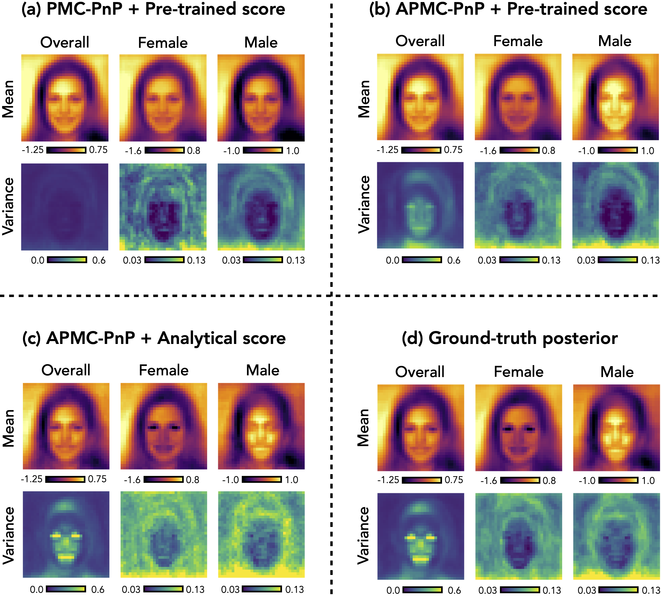
Figure 2: Comparison of the sample statistics obtained by PMC-PnP and APMC-PnP versus the ground-truth posterior distribution. Each test algorithm is run to collect $1000$ samples, which are then classified into two modes according to their distance and angle with respect to the ground-truth modes. PMC-PnP, which does not use annealing, fails to identify the bimodal distribution, as can be seen by the two groups of classified images being nearly indistinguishable. Under the pre-trained score, APMC-PnP significantly improves in performance over PMC-PnP by distinguishing the female and male modes. These two modes look similar to the ground truth posterior modes, although some differences remain due to the use of an approximate learned score. In the ideal case of the analytical score, APMC-PnP recovers a distribution that closely resembles the ground-truth posterior.

Fig. 2 compares the sampling performance of APMC-PnP and PMC-PnP against ground-truth posterior. All algorithms are run until convergence to sample $1000$ images, and we use a large non-divergent step-size to accelerate the procedure. Fig. 2(a) and 2(b) compares the PMC-PnP and APMC-PnP under the pre-trained score. It is clear that the PMC-PnP struggles in sampling the two modes, leading to a unitary cluster of samples that are inseparable. On the contrary, APMC-PnP can successfully capture the two modes by leveraging weighted annealing. Note the improvement in the overall and per-mode statistics led by APMC-PnP. When the analytical score is used, Fig. 2(c) and 2(d) display almost identical overall statistics, demonstrating the high-quality recovery of the posterior distribution by APMC-PnP. Note the closeness between the means of APMC-PnP and groundtruth. However, we notice that APMC-PnP tends to get larger sample variances for each mode. This might be attributed to the large step-size and could be mitigated by using smaller values.

6 Experiments on Imaging Inverse Problems

In this section, we demonstrate the performance of APMC algorithms on real-world imaging inverse problems. Our experiments consist of three high-dimensional image recovery tasks: compressed sensing (CS), magnetic resonance imaging (MRI), and black-hole interferometric imaging (BHI). Together, these tasks provide coverage of both log-concave and non-log-concave likelihoods.

6.1 Score-based generative priors

To fully leverage the latest advances in SGM, we implement our score network by customizing the state-of-the-art U-Net architecture in guided diffusion [55]. We introduce a key modification to make the network take the smoothing strength $\sigma$ as input by leveraging techniques in [56]. We train individual networks for approximating the scores of three image prior distributions, that is, human face images, brain MRI images, and black-hole images, which are used in the experiments of CS, MRI, and BHI, respectively. Note that the training of the score network is agnostic to the forward models of these imaging tasks. We train the score network over the smoothing ranges $\sigma\in[348,0.01]$ and $\sigma\in[192,0.01]$ for $256\times 256$ and $64\times 64$ images, respectively. Note that these ranges are suggested by [56] for achieving the optimized performance. We refer to Supplement II for additional technical details on the architecture and training.

6.2 Linear Inverse Problems: CS and MRI

The inverse problems of CS and MRI that we tackle can be described by a linear version of the system in (2), where $\Abm$ corresponds to either a i.i.d random Gaussian matrix or the Fourier transform with subsampling, and $\ebm$ corresponds to 40 dB input signal-to-noise ratio (SNR). Both tasks are performed on a dataset of $40$ images with the spatial resolution of $256\times 256$ pixels, where $10$ held-out images are used for finetuning the hyperparameters, and the remaining $30$ images are used for collecting the test results. All images are normalized to $[-1,1]$. We include four baseline methods for comparison: PnP, RED, PnP-ULA [26], and DPS [22]. The first two algorithms correspond to MAP-based methods, while the rest are designed for posterior sampling. In the test, PnP and RED are equipped with the pre-trained DnCNN denoisers from [57], while PnP-ULA and DPS use the score networks. We refer to Supplement II for the details on the implementation of baseline methods. In each experiment, we run algorithms for a maximum number of $10,000$ iterations to collect the final results. For the sampling methods, the final reconstructed image is obtained by averaging $10$ image samples.

We evaluate the reconstruction quality by using the peak signal-to-noise ratio (PSNR), which is inversely related to the mean squared error (MSE). We use PSNR as the criterion to finetune the algorithmic hyperparameters. To quantitatively measure the quality of UQ, we compute the normalized negative log-likelihood (NLL) [58] of the groundtruth $\xbm$ under independent pixel-wise Gaussian distributions characterized by the sample mean $\xbmbar$ and standard deviation $\mathsf{SD}$

$$\mathsf{NLL}(\xbmbar,\xbm)=\frac{1}{n}\sum_{i=1}^{n}\frac{1}{2\mathsf{SD}^{2}_{i}}(\xbmbar_{i}-\xbm_{i})^{2}+\frac{1}{2}\log(2\pi\mathsf{SD}^{2}_{i})$$ (21)

where $i$ is the pixel index and $\mathsf{SD}_{i}$ the $i$th estimated standard deviation. It follows that better UQ algorithms minimize NLL by producing a high-fidelity $\xbmbar$ and avoiding the need for an arbitrarily large $\mathsf{SD}$. We additionally calculate the pixel-wise 3-SD credible interval to measure the coverage of the groundtruth. If the distribution were truly Gaussian, $99\%$ of the ground-truth pixels should lie within the 3-SD interval; however, as our posterior distributions are not Gaussian with a score-based prior, we do not expect to reach $99\%$ coverage in our experiments.

6.2.1 Compressed Sensing

Two different CS ratios $(m/n)$ of $\{10\%,30\%\}$ are considered in the experiments. We train the score network using the FFHQ dataset [59], while randomly selecting the test images from the separate CelebA dataset [54].

Table LABEL:Tab:Recon ($m/n=0.1$ & $m/n=0.3$) summarize the averaged PSNR and MSE values obtained by all algorithms. First, the table clearly shows the substantial improvement led by APMC algorithms over the baselines in all settings. In particular, when the compression is severe ($m/n=0.1$), APMC algorithms achieve around $28.10$ dB in averaged PSNR, outperforming the best baseline by $3.18$ dB. The enhancement is further demonstrated in the visual comparison shown in Fig. LABEL:Fig:Recon (1st row). We observe that APMC algorithms can faithfully recover fine details preserved in the groundtruth. In particular, note the hair, teeth, and eye shape highlighted in the zoom-in regions. Second, the poor results of PnP-ULA imply the slow convergence of stationary Langevin algorithms. We run PnP-ULA on one test image for more iterations and fail to observe convergence within $30,000$ iterations under both settings (see Supplement III for the convergence plots). On the other hand, APMC algorithms generally converge within $4,000$ iterations, showing a significant acceleration in speed led by weighted annealing in this CS task.

Table LABEL:Tab:UQ ($m/n=0.1$ & $m/n=0.3$) summarize the averaged NLL values obtained by the APMC algorithms and sampling baselines. We additionally summarize the averaged pixel-wise absolute error ($|\xbmbar-\xbm|$) and standard deviation (SD) as they are the two factors that jointly determine the final value of NLL. Beyond high-quality reconstruction, the results show that APMC algorithms also achieve better UQ performance than the baselines, by simultaneously producing a high-fidelity mean and avoiding the need for a large SD. Fig. LABEL:Fig:UQ(a) visualizes the pixel-wise statistics associated with the reconstruction in Fig LABEL:Fig:Recon (1st row). In the left columns, we plot the 3-SD credible interval where the outside pixels are highlighted in red. Note that around $97\%$ of the pixels in the ground-truth image lie in the 3-SD interval from the reconstructions produced by APMC algorithms. Despite DPS also achieving a high coverage ratio, it yields inaccurate $\xbmbar$ and thus large SD which leads to poor NLL performance.

6.2.2 Magnetic resonance imaging

In this task, we consider the radial subsampling mask corresponding to $\{4\times,8\times\}$ acceleration. We use the FastMRI dataset [60] to train the score network and to form the testing dataset.

Table LABEL:Tab:Recon and LABEL:Tab:UQ ($\text{Accel.}=8\times$ & $\text{Accel.}=4\times$) summarize the numerical performance of all algorithms in image reconstruction and UQ, respectively. Overall, the APMC algorithms still yield the best PSNR and NLL values, showing consistent performance across different inverse problems. On the other hand, we observe the convergence of PnP-ULA under $4\times$ acceleration, which is reflected in the better numerical values. This fact shows that the stationary Langevin algorithms are able to sample from the posterior but require more iterations. Fig. LABEL:Fig:Recon (2nd row) provides a visual comparison of the reconstructed images under $8\times$ acceleration, and Fig. LABEL:Fig:UQ(b) visualizes the associated pixel-wise statistics. Note how APMC algorithms restore the fine features in different brain areas and cover about $99\%$ of the ground-truth pixels with a narrower 3-SD credible interval.

We additionally compare APMC algorithms with the state-of-the-art end-to-end VarNet [61] in terms of the reconstruction quality. By just leveraging the model-agnostic priors, both APMC algorithms demonstrate close results to the VarNet which requires model-specific training. We refer to Supplement III for a detailed discussion.

Figure 3: Visual illustration of BHI. The left two images together demonstrate the subsampling pattern in the Fourier spectrum. The Groundtruth image shows the ground-truth black hole simulation image used in this experiment. The Target image corresponds to the scenario where the low-frequency band is fully sampled, resembling a single-dish telescope the size of the Earth. This target image represents the intrinsic resolution of our telescope; an effort to recover sharper features would be classified as attempting superresolution.

6.3 Nonlinear black-hole interferometric imaging

We now validate APMC algorithms on the nonlinear BHI task. The imaging system of BHI can be mathematically characterized by the van Cittert-Zernike theorem, which links each Fourier component, or so-called visibility, of the black-hole image to the coherence measured by a pair of telescopes. The measurement equation for each visibility is given by

$$V_{a,b}^{t}=g_{a}^{t}g_{b}^{t}\cdot e^{-i(\phi_{a}^{t}-\phi_{b}^{t})}\cdot\tilde{\Ibm}_{a,b}^{t}(\xbm)+\eta_{a,b}$$ (22)

where $a$ and $b$ index the telescopes, $t$ represents time, and $\tilde{\Ibm}_{a,b}^{t}(\xbm)$ is the ideal Fourier component of image $\xbmast$ corresponding to the baseline between telescopes $a$ and $b$ at time $t$. In practice, the visibility is corrupted by three types of noise: telescope-based gain error $g_{a}$ and $g_{b}$, telescope-based phase error $\phi_{a}^{t}$ and $\phi_{a}^{t}$, and baseline-based AWGN $\eta_{a,b}$. The first two types of noise are usually caused by atmospheric turbulence and instrument miscalibration, while the last one corresponds to thermal noise. To mitigate the gain and phase error, multiple noisy visibilities are combined into noise-canceling data products termed closure phases and log closure amplitudes

$$\ybm^{\mathsf{cph}}_{t,(a,b,c)}=\angle(V_{a,b}V_{b,c}V_{a,c})$$ (23)

$$\ybm^{\mathsf{camp}}_{t,(a,b,c,d)}=\log\left(\frac{|V_{a,b}^{t}||V_{c,d}^{t}|}{|V_{a,c}||V_{b,d}^{t}|}\right)$$ (24)

where $\angle$ computes the angle of a complex number. Given total $M>0$ telescopes, the number of combined measurements $\ybm^{\mathsf{cph}}_{t}$ and $\ybm^{\mathsf{camp}}_{t}$ at time $t$ are given by $\frac{(M-1)(M-2)}{2}$ and $\frac{M(M-3)}{2}$, respectively, after excluding repetitive measurements. Here, we adopt a 9-telescope array ($M=9$) consisting of telescopes that currently participate in the Event Horizon Telescope (EHT). In summary, the forward problem of BHI is formulated as

$$\begin{cases}\ybm^{\mathsf{cph}}_{t}=\Abm^{\mathsf{cph}}_{t}(\xbm)\\ \ybm^{\mathsf{camp}}_{t}=\Abm^{\mathsf{camp}}_{t}(\xbm)\end{cases}\text{where}\;\begin{cases}\Abm^{\mathsf{cph}}_{t}=(\Abm^{\mathsf{cph}}_{t,\mathsf{c}_{1}},\cdots,\Abm^{\mathsf{cph}}_{t,\mathsf{c}_{k_{1}}})^{T}\\ \Abm^{\mathsf{camp}}_{t}=(\Abm^{\mathsf{camp}}_{t,\mathsf{c}_{1}},\cdots,\Abm^{\mathsf{camp}}_{t,\mathsf{c}_{k_{2}}})^{T}\end{cases}$$

Note that the inverse problem of BHI is severely ill-posed: even if we have an Earth-size telescope, the high-frequency visibilities are still immeasurable; in practice, the low-frequency band is further subsampled. A visual illustration of BHI is provided in Fig. 3. Additionally, the gain and phase errors result in significant information loss; for instance, the absolute phase of the image can never be recovered and the total flux (i.e. summation of the pixel values) of the image is not constrained by either of the closure quantities. Since this is the case we include an additional constraint in the likelihood to constrain the total flux:

$$\ell(\ybm|\xbm)= \underbrace{\sum_{t,\mathsf{c}}\frac{\|\Abm^{\mathsf{cph}}_{t,\mathsf{c}}(\xbm)-\ybm^{\mathsf{cph}}_{t,\mathsf{c}}\|^{2}_{2}}{2\beta_{\mathsf{cph}}^{2}}}_{\chi^{2}_{\mathsf{cph}}}+\underbrace{\sum_{t,\mathsf{c}}\frac{\|\Abm^{\mathsf{camp}}_{t,\mathsf{c}}(\xbm)-\ybm^{\mathsf{camp}}_{t,\mathsf{c}}\|_{2}^{2}}{2\beta_{\mathsf{camp}}^{2}}}_{\chi^{2}_{\mathsf{camp}}}$$

$$+\rho\frac{\left\|\sum_{i}\xbm_{i}-\ybm^{\mathsf{flux}}\right\|_{2}^{2}}{2},$$ (25)

where $\beta_{\mathsf{cph}}$ and $\beta_{\mathsf{camp}}$ are assumed to be known, $\ybm^{\mathsf{flux}}$ can be accurately measured, and $\rho>0$ is an optimization parameter. The first two terms in (6.3) are referred to as the $\chi^{2}$ errors.

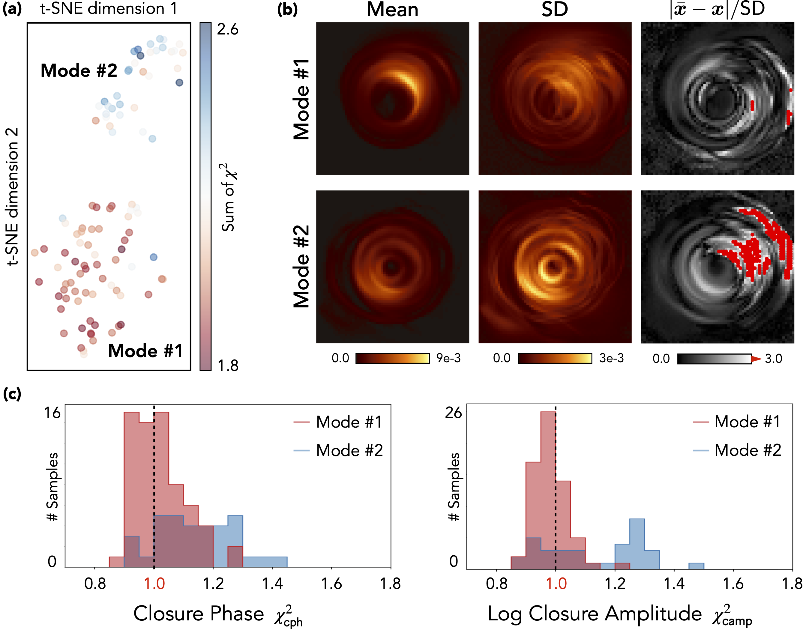
Figure 4: Visualization of the sampling results obtained by APMC-PnP. In total $100$ samples were drawn. (a) The t-SNE plot (perplexity=20) shows the distribution of the samples. Note that this t-SNE plot shows there are two distinct image modes. (b) Pixel-wise statistics of each mode. (c) The distribution of the closure phase $\chi^{2}_{\mathsf{cph}}$ and log closure amplitude $\chi^{2}_{\mathsf{camp}}$ statistics for each mode. Note that APMC-PnP successfully recovers the two modes of the posterior distribution, with both modes resulting in $\chi^{2}$ statistics close to 1.

Experimental setup

We test our APMC algorithms on a synthetic BHI problem that has previously been shown to lead to a bimodal posterior distribution [19]. The ground-truth test image is shown in Fig. 3. One of the primary objectives of this experiment is to determine if the algorithms can successfully reconstruct this bimodal distribution. We additionally assess the fidelity of the reconstruction using the $\chi^{2}$ errors. Note that $\chi^{2}_{\mathsf{cph}}=\chi^{2}_{\mathsf{camp}}=1$ indicates that the measurements and prior are ideally balanced.

We use the GRMHD dataset [62] to train the score network. All images used in the experiment are resized to $64\times 64$ pixels. We observe that APMC-PnP and APMC-RED yield identical results for BHI as the step-size allowed for convergence is small ($10^{-6}$); hence, we restrict our discussion to the results of APMC-PnP for brevity. We include DPI with a score-based prior (scoreDPI) [20, 47] as the baseline method. We run each algorithm to draw $100$ samples for computing the final results. Note that scoreDPI is a variational method and needs to be retrained for different test cases. Additionally, due to computational and memory constraints, an approximation of the prior log-density must be used in scoreDPI in order to handle $64\times 64$ images.

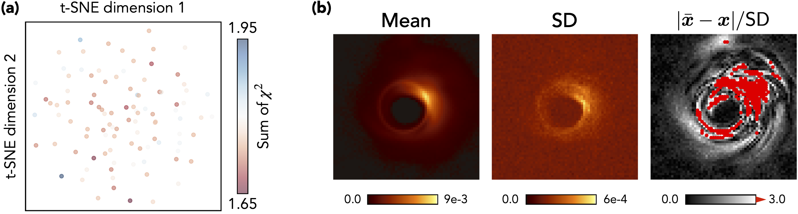
Figure 5: Visualization of the sampling results obtained by scoreDPI. (a) shows the t-SNE plot (perpelxity=20), and (b) plots the sample statistics. Note that scoreDPI recovers a single-mode distribution rather than a bimodal distribution.

Results

Fig. 4 visualizes the statistics of the samples generated by APMC-PnP. We use the t-distributed stochastic neighbor embedding (t-SNE) to plot the distribution of the samples. As shown in Fig. 4(a), the samples can be classified into two modes: Mode #1 is composed of the black holes with their flux concentrating in the top-right corner (as is also the case in the groundtruth), while the black holes from Mode #2 have the flux concentration at the bottom-left corner. Our result is aligned with the previous experiment that recovered two similar modes (see Fig. 6 in [19]). The uncertainty of each mode is shown in Fig. 4(b). Note the almost full coverage of the groundtruth by the 3-SD credible interval of Mode #1. Fig. 4(c) illustrates the data-fidelity for each sample by plotting the histogram of the $\chi^{2}_{\mathsf{cph}}$ and $\chi^{2}_{\mathsf{camp}}$ errors. We highlight that the values obtained by both modes are distributed close to 1. Fig. 5 visualizes the statistics for scoreDPI. The t-SNE plot shows that scoreDPI recovers a single-mode distribution rather than a bimodal distribution. The inability of scoreDPI to recover the bimodal distribution could be caused by a few factors that potentially lead to inaccurate posterior estimation: 1) the posterior is approximated by a normalizing flow network that likely struggles to model the rich posterior of $64\times 64$ pixel images, and 2) to handle this image size an approximation to the prior log-density was used. In contrast, our method does not suffer from these factors and can handle large image sizes without making additional approximations. We also note that there is less coverage of the ground-truth pixels within 3-SD interval of scoreDPI when compared with Mode #1’s result obtained by APMC-PnP.

7 Conclusion

In this paper, we develop PMC as a principled posterior sampling framework for solving general imaging inverse problems. PMC jointly leverages the expressive score-based generative priors and physical constraints while also enabling the UQ of the reconstructed image via posterior sampling. In particular, we introduce two PMC algorithms which can be backward-related to the traditional PnP and RED algorithms. A comprehensive convergence analysis for both stationary and annealed variants of the PMC algorithms is presented. Our results show that all algorithms converge at the rate of $O(1/N)$. Related experiments are also presented to empirically confirm the proposed theorems and to elucidate the capability of PMC in various representative inverse problems, including a non-convex problem that leads to a bimodal posterior distribution.

Supplementary Material

8 Technical Proofs

In this section, we present the technical proofs. The general idea of our proof is inspired by the interpolation technique used in [63, 53]. In order to analyze the convergence of a PMC algorithm (which is discrete in time), we follow [53] to “linearly” interpolate the iterations of the algorithm, forming a corresponding continuous-time diffusion process. By doing so, we are able to use tools in continuous mathematics such as differential inequalities to study the change of the Kullback–Leibler (KL) divergence along the interpolated diffusion process. Indeed, the interpolated diffusion process can be understood as a “piece-wise constant” gradient flow of the KL divergence in the space of probability distributions. Therefore, we can follow the practice in optimization to derive the stationary-distribution convergence. Here, the stationary condition will be given in terms of the relative Fisher information (FI), which measures the norm of the “gradient” of KL divergence under the Wasserstein metric.

This section is organized as follows. In Subsection LABEL:Sec:Lemmas, we present two lemmas that we adapted from [53]; we also introduce some simpler proof of these lemmas. With the two lemmas, we prove the main theorem of our paper in Subsections LABEL:Sec:Proof1, LABEL:Sec:Proof2, LABEL:Sec:Proof3, and LABEL:Sec:Proof4.

Notations  Throughout the proof, we consider the probability space $(\Omega,\Fscr,\mathbb{P})$, where $\Omega$ denotes the sample space, $\Fscr$ the $\sigma$-algebra, and $\mathbb{P}$ the probability measure. For the random variable $\zeta:\Omega\rightarrow\R^{n}$, we denote its expectation by $\E[\zeta]=\int_{\Omega}\zeta(\omega)\mathbb{P}(d\omega)$.

We recall that the posterior distribution that we are interested in takes the form $\pi(\xbm|\ybm)\propto\ell(\ybm|\xbm)p(\xbm)$. We define $g(\xbm)=-\log\ell(\ybm|\xbm)$ . For ease of notation, we will omit the presence of $\ybm$ and simply write $\pi(\xbm|\ybm)$ by $\pi(\xbm)$ in our proof. As a reminder, we have the following relations:

$$\pi\propto e^{-f},\quad\nabla f=-\nabla\log\pi=\nabla g-\nabla\log p\,.$$

Here, we assume $\nabla f\in C^{1}$ is differentiable and has a continuous derivative. We will use the above notations and relations constantly in the proof. For reader’s convenience, we recall the definition of the KL divergence for two probability densities $\nu$ and $\pi$ is ( ν ∥  π

References

- [1] L. I. Rudin, S. Osher, and E. Fatemi, “Nonlinear total variation based noise removal algorithms,” Physica D, vol. 60, pp. 259–268, Nov. 1992.
- [2] A. Beck and M. Teboulle, “Fast gradient-based algorithm for constrained total variation image denoising and deblurring problems,” IEEE Trans. Image Process., vol. 18, pp. 2419–2434, November 2009.
- [3] S. V. Venkatakrishnan, C. A. Bouman, and B. Wohlberg, “Plug-and-play priors for model based reconstruction,” in Proc. IEEE Global Conf. Signal Process. and Inf. Process. (GlobalSIP), (Austin, TX, USA), pp. 945–948, Dec. 3-5, 2013.
- [4] Y. Romano, M. Elad, and P. Milanfar, “The little engine that could: Regularization by denoising (RED),” SIAM J. Imaging Sci., vol. 10, no. 4, pp. 1804–1844, 2017.
- [5] Z. Wu, Y. Sun, A. Matlock, J. Liu, L. Tian, and U. S. Kamilov, “Simba: Scalable inversion in optical tomography using deep denoising priors,” Oct. 2019.
- [6] R. Ahmad, C. A. Bouman, G. T. Buzzard, S. Chan, S. Liu, E. T. Reehorst, and P. Schniter, “Plug-and-play methods for magnetic resonance imaging: Using denoisers for image recovery,” IEEE Signal Process. Mag., vol. 37, no. 1, pp. 105–116, 2020.
- [7] K. Zhang, Y. Li, W. Zuo, L. Zhang, L. Van Gool, and R. Timofte, “Plug-and-play image restoration with deep denoiser prior,” IEEE Transactions on Pattern Analysis and Machine Intelligence, vol. 44, no. 10, pp. 6360–6376, 2022.
- [8] J. M. Bardsley, “Mcmc-based image reconstruction with uncertainty quantification,” SIAM Journal on Scientific Computing, vol. 34, no. 3, pp. A1316–A1332, 2012.
- [9] A. Repetti, M. Pereyra, and Y. Wiaux, “Scalable bayesian uncertainty quantification in imaging inverse problems via convex optimization,” SIAM Journal on Imaging Sciences, vol. 12, no. 1, pp. 87–118, 2019.
- [10] L. Yang, Z. Zhang, Y. Song, S. Hong, R. Xu, Y. Zhao, W. Zhang, B. Cui, and M.-H. Yang, “Diffusion models: A comprehensive survey of methods and applications,” 2023.
- [11] S. Boyd, N. Parikh, E. Chu, B. Peleato, and J. Eckstein, “Distributed optimization and statistical learning via the alternating direction method of multipliers,” Found. Trends Mach. Learn., vol. 3, no. 1, pp. 1–122, 2011.
- [12] A. Beck and M. Teboulle, “A fast iterative shrinkage-thresholding algorithm for linear inverse problems,” SIAM J. Imaging Sci., vol. 2, no. 1, pp. 183–202, 2009.
- [13] U. S. Kamilov, H. Mansour, and B. Wohlberg, “A plug-and-play priors approach for solving nonlinear imaging inverse problems,” IEEE Signal. Proc. Let., vol. 24, pp. 1872–1876, Dec. 2017.
- [14] C. A. Metzler, A. Maleki, and R. G. Baraniuk, “From denoising to compressed sensing,” IEEE Trans. Inf. Theory, vol. 62, pp. 5117–5144, September 2016.
- [15] S. Ono, “Primal-dual plug-and-play image restoration,” IEEE Signal Process. Lett., vol. 24, no. 8, pp. 1108–1112, 2017.
- [16] Y. Sun, Z. Wu, X. Xu, B. Wohlberg, and U. S. Kamilov, “Scalable plug-and-play admm with convergence guarantees,” IEEE Transactions on Computational Imaging, vol. 7, pp. 849–863, 2021.
- [17] U. S. Kamilov, C. A. Bouman, G. T. Buzzard, and B. Wohlberg, “Plug-and-play methods for integrating physical and learned models in computational imaging: Theory, algorithms, and applications,” IEEE Signal Processing Magazine, vol. 40, no. 1, pp. 85–97, 2023.
- [18] E. T. Reehorst and P. Schniter, “Regularization by denoising: Clarifications and new interpretations,” IEEE Trans. Comput. Imag., vol. 5, pp. 52–67, Mar. 2019.
- [19] H. Sun and K. L. Bouman, “Deep probabilistic imaging: Uncertainty quantification and multi-modal solution characterization for computational imaging,” in AAAI Conference on Artificial Intelligence (AAAI), 2021.
- [20] B. T. Feng, J. Smith, M. Rubinstein, H. Chang, K. L. Bouman, and W. T. Freeman, “Score-based diffusion models as principled priors for inverse imaging,” 2023.
- [21] Y. Song, L. Shen, L. Xing, and S. Ermon, “Solving inverse problems in medical imaging with score-based generative models,” in International Conference on Learning Representations, 2022.
- [22] H. Chung, J. Kim, M. T. Mccann, M. L. Klasky, and J. C. Ye, “Diffusion posterior sampling for general noisy inverse problems,” in The Eleventh International Conference on Learning Representations, 2023.
- [23] J. Liu, R. Anirudh, J. J. Thiagarajan, S. He, K. A. Mohan, U. S. Kamilov, and H. Kim, “Dolce: A model-based probabilistic diffusion framework for limited-angle CT reconstruction,” in Proc. IEEE Int. Conf. Comp. Vis. (ICCV), 2023.
- [24] A. Jalal, M. Arvinte, G. Daras, E. Price, A. G. Dimakis, and J. Tamir, “Robust compressed sensing mri with deep generative priors,” in Advances in Neural Information Processing Systems, vol. 34, pp. 14938–14954, 2021.
- [25] B. Kawar, G. Vaksman, and M. Elad, “SNIPS: Solving noisy inverse problems stochastically,” in Advances in Neural Information Processing Systems, 2021.
- [26] R. Laumont, V. D. Bortoli, A. Almansa, J. Delon, A. Durmus, and M. Pereyra, “Bayesian imaging using plug & play priors: When langevin meets tweedie,” SIAM Journal on Imaging Sciences, vol. 15, no. 2, pp. 701–737, 2022.
- [27] F. Coeurdoux, N. Dobigeon, and P. Chainais, “Plug-and-play split gibbs sampler: embedding deep generative priors in bayesian inference,” 2023.
- [28] C. A. Bouman and G. T. Buzzard, “Generative plug and play: Posterior sampling for inverse problems,” 2023.
- [29] S. H. Chan, X. Wang, and O. A. Elgendy, “Plug-and-play ADMM for image restoration: Fixed-point convergence and applications,” IEEE Trans. Comput. Imag., vol. 3, pp. 84–98, Mar. 2017.
- [30] Y. Sun, B. Wohlberg, and U. S. Kamilov, “An online plug-and-play algorithm for regularized image reconstruction,” IEEE Trans. Comput. Imag., vol. 5, pp. 395–408, Sept. 2019.
- [31] E. K. Ryu, J. Liu, S. Wang, X. Chen, Z. Wang, and W. Yin, “Plug-and-play methods provably converge with properly trained denoisers,” in Proc. 36th Int. Conf. Machine Learning (ICML), vol. 97, pp. 5546–5557, 2019.
- [32] R. G. Gavaskar and K. N. Chaudhury, “Plug-and-Play ISTA converges with kernel denoisers,” IEEE Signal Process. Lett., vol. 27, pp. 610–614, Apr. 2020.
- [33] X. Xu, Y. Sun, J. Liu, B. Wohlberg, and U. S. Kamilov, “Provable convergence of plug-and-play priors with mmse denoisers,” IEEE Signal Process. Lett., vol. 27, pp. 1280–1284, 2020.
- [34] P. Nair, R. G. Gavaskar, and K. N. Chaudhury, “Fixed-point and objective convergenceof plug-and-play algorithms,” IEEE Trans. Comput. Imag., vol. 7, pp. 337–348, 2021.
- [35] R. Cohen, M. Elad, and P. Milanfar, “Regularization by denoising via fixed-point projection (RED-PRO),” arXiv:2008.00226 [eess.IV], 2020.
- [36] Y. Sun, J. Liu, and U. S. Kamilov, “Block coordinate regularization by denoising,” in Advances in Neural Information Processing Systems 32, pp. 380–390, 2019.
- [37] Z. Wu, Y. Sun, A. Matlock, J. Liu, L. Tian, and U. S. Kamilov, “SIMBA: Scalable inversion in optical tomography using deep denoising priors,” IEEE J. Sel. Topics Signal Process., pp. 1–1, 2020.
- [38] Y. Sun, J. Liu, Y. Sun, B. Wohlberg, and U. Kamilov, “Async-RED: A provably convergent asynchronous block parallel stochastic method using deep denoising priors,” in International Conference on Learning Representations (ICLR), 2021.
- [39] Y. Hu, J. Liu, X. Xu, and U. S. Kamilov, “Monotonically convergent regularization by denoising,” in 2022 IEEE International Conference on Image Processing (ICIP), pp. 426–430, 2022.
- [40] R. Laumont, V. De Bortoli, A. Almansa, J. Delon, A. Durmus, and M. Pereyra, “On maximum a posteriori estimation with plug & play priors and stochastic gradient descent,” Journal of Mathematical Imaging and Vision, vol. 65, no. 1, pp. 140–163, 2023.
- [41] Y. Song and S. Ermon, “Generative modeling by estimating gradients of the data distribution,” in Advances in Neural Information Processing Systems, vol. 32, 2019.
- [42] J. Ho, A. Jain, and P. Abbeel, “Denoising diffusion probabilistic models,” in Advances in Neural Information Processing Systems (H. Larochelle, M. Ranzato, R. Hadsell, M. Balcan, and H. Lin, eds.), vol. 33, pp. 6840–6851, 2020.
- [43] Y. Song, J. Sohl-Dickstein, D. P. Kingma, A. Kumar, S. Ermon, and B. Poole, “Score-based generative modeling through stochastic differential equations,” in International Conference on Learning Representations, 2021.
- [44] B. Efron, “Tweedie’s formula and selection bias,” Journal of the American Statistical Association, vol. 106, no. 496, pp. 1602–1614, 2011.
- [45] P. Vincent, “A connection between score matching and denoising autoencoders,” Neural Comput., vol. 23, no. 7, pp. 1661–1674, 2011.
- [46] D. P. Kingma and M. Welling, “Auto-encoding variational bayes,” arXiv:1312.6114, 2013.
- [47] B. T. Feng and K. L. Bouman, “Efficient bayesian computational imaging with a surrogate score-based prior,” arXiv preprint arXiv:2309.01949, 2023.
- [48] G. Cardoso, Y. J. E. Idrissi, S. L. Corff, and E. Moulines, “Monte carlo guided diffusion for bayesian linear inverse problems,” arXiv:2308.07983, 2023.
- [49] R. Jordan, D. Kinderlehrer, and F. Otto, “The variational formulation of the fokker–planck equation,” SIAM Journal on Mathematical Analysis, vol. 29, no. 1, pp. 1–17, 1998.
- [50] R. M. Neal, “Annealed importance sampling,” Statistics and Computing, vol. 11, no. 2, pp. 125–139, 2001.
- [51] C. Villani et al., Optimal transport: old and new, vol. 338. Springer, 2009.
- [52] L. Ambrosio, N. Gigli, and G. Savaré, Gradient Flows in Metric Spaces and in the Space of Probability Measures. Lectures in Mathematics ETH Zürich, Birkhäuser, 2008.
- [53] K. Balasubramanian, S. Chewi, M. A. Erdogdu, A. Salim, and S. Zhang, “Towards a theory of non-log-concave sampling:first-order stationarity guarantees for langevin monte carlo,” in Proceedings of Thirty Fifth Conference on Learning Theory, vol. 178, pp. 2896–2923, 02–05 Jul 2022.
- [54] Z. Liu, P. Luo, X. Wang, and X. Tang, “Deep learning face attributes in the wild,” in Proceedings of International Conference on Computer Vision (ICCV), 2015.
- [55] P. Dhariwal and A. Q. Nichol, “Diffusion models beat GANs on image synthesis,” in Advances in Neural Information Processing Systems, 2021.
- [56] Y. Song and S. Ermon, “Improved techniques for training score-based generative models,” in Advances in Neural Information Processing Systems 33, 2020.
- [57] K. Zhang, W. Zuo, Y. Chen, D. Meng, and L. Zhang, “Beyond a Gaussian denoiser: Residual learning of deep CNN for image denoising,” IEEE Trans. Image Process., vol. 26, pp. 3142–3155, July 2017.
- [58] B. Lakshminarayanan, A. Pritzel, and C. Blundell, “Simple and scalable predictive uncertainty estimation using deep ensembles,” Advances in neural information processing systems, vol. 30, 2017.
- [59] T. Karras, S. Laine, and T. Aila, “A style-based generator architecture for generative adversarial networks,” in 2019 IEEE/CVF Conference on Computer Vision and Pattern Recognition (CVPR), pp. 4396–4405, 2019.
- [60] Zbontar et al., “fastMRI: An open dataset and benchmarks for accelerated MRI,” 2018. arXiv:1811.08839.
- [61] A. Sriram, J. Zbontar, T. Murrell, A. Defazio, C. L. Zitnick, N. Yakubova, F. Knoll, and P. Johnson, “End-to-end variational networks for accelerated mri reconstruction,” in Medical Image Computing and Computer Assisted Intervention, pp. 64–73, 2020.
- [62] G. N. Wong, B. S. Prather, V. Dhruv, B. R. Ryan, M. Mościbrodzka, C. kwan Chan, A. V. Joshi, R. Yarza, A. Ricarte, H. Shiokawa, J. C. Dolence, S. C. Noble, J. C. McKinney, and C. F. Gammie, “Patoka: Simulating electromagnetic observables of black hole accretion,” The Astrophysical Journal Supplement Series, vol. 259, no. 2, p. 64, 2022.
- [63] S. Vempala and A. Wibisono, “Rapid convergence of the unadjusted langevin algorithm: Isoperimetry suffices,” in Advances in Neural Information Processing Systems 32, 2019.
- [64] S. Chewi, M. A. Erdogdu, M. Li, R. Shen, and S. Zhang, “Analysis of langevin monte carlo from poincare to log-sobolev,” in Proceedings of Thirty Fifth Conference on Learning Theory (P.-L. Loh and M. Raginsky, eds.), vol. 178, pp. 1–2, 02–05 Jul 2022.