Deep Policy Iteration for High-Dimensional Mean Field Games

Abstract

This paper introduces Deep Policy Iteration (DPI), a novel approach that combines the MFDGM [1] method and the Policy Iteration method [2, 3] to address high-dimensional stochastic Mean Field Games. The Deep Policy Iteration employs three neural networks to approximate the solutions of equations. These networks are trained to satisfy each equation and its corresponding forward-backward conditions. Unlike existing approaches that are limited to separable Hamiltonians and lower dimensions, DPI extends its capabilities to effectively solve high-dimensional MFG systems, encompassing both separable and non-separable Hamiltonians. To evaluate the reliability and efficacy of DPI, a series of numerical experiments is conducted. The results obtained using DPI are compared with those obtained using the MFDGM method and the Policy Iteration Method. This comparative analysis provides insights into the performance of DPI and its advantages over existing methods.

latexText page 7 contains only floats

[inst1]organization=College of Computing, UM6P,addressline=Lot 660, city=BenGuerir, postcode=43150, country=Morocco

[inst2]organization=College of Computing, UM6P,addressline=Lot 660, city=BenGuerir, postcode=43150, country=Morocco

1 Introduction

Mean Field Games (MFG) theory, introduced by Lasry and Lions [4], provides a framework for analyzing Nash equilibria in differential games involving a large number of agents. This theory is characterized by a mathematical formulation consisting of a system of coupled partial differential equations (PDEs). Specifically, the system comprises a forward-time Fokker-Planck equation (FP) and a backward-time Hamilton-Jacobi-Bellman equation (HJB), which govern the evolution of the population density and the value function, respectively. MFGs have garnered significant attention and have been extensively studied in various fields, such as autonomous vehicles [5, 6], finance [7, 8], economics [9, 10, 11]. In the general case, the MFG system is described as,

$$\left\{\begin{array}[]{rrrrr}-\partial_{t}\phi-\nu\Delta\phi+H(x,\rho,\nabla\phi)=0,\ in&E,\\ \partial_{t}\rho-\nu\Delta\rho-\operatorname{div}\left(\rho\nabla_{p}H(x,\rho,\nabla\phi)\right)=0,\ in&E,\\ \rho(0,x)=\rho_{0}(x),\ \ \phi(T,x)=g(x,\rho(T,x)),\ in&\Omega,\end{array}\right.$$ (1)

where, $E=[0,T]\times\Omega,$ $\Omega$ bounded subset of $\mathbb{R}^{d}$ and $g$ denotes the terminal cost. The Hamiltonian $H$ with separable structure is defined as

$$H(x,\rho,p)=inf_{v}\{-p.v+L_{0}(x,v)\}-f_{0}(x,\rho)=H_{0}(x,p)-f_{0}(x,\rho),$$ (2)

The solution of (1) exists and is unique under the standard assumptions of convexity of $H$ in the second variable and monotonicity of $f$ and $g$ [12], see also refs [13, 4] for more details. For non-separable Hamiltonians, where the Hamiltonian of the MFG depends jointly on $\rho$ and $p$, the existence and uniqueness of the solution for MFGs of congestion type has been investigated by Achdou and Porretta in [14] and Gomes et al. in [15].

The numerical solution of (1) holds significant importance in the practical application of MFG theory. However, due to the strong coupling and forward-backward structure of the two equations in (1), they cannot be solved independently or jointly using simple forward-in-time methods. Extensive research has been conducted in this area, leading to the proposal of various methods with successful applications, as seen in [16, 4] and references therein. Nevertheless, these methods often face challenges in terms of computational complexity, particularly when dealing with high-dimensional problems [17, 18].

To address this challenge, deep learning methods, such as Generative Adversarial Networks (GANs) [12, 19], have been utilized to reformulate MFGs as primal-dual problems. However, these existing methods require the Hamiltonian $H$ to be separable in terms of $\rho$ and $p$. Unfortunately, none of these methods adequately cover the case of a non-separable Hamiltonian with a generic structure.

To the best of our knowledge, two promising numerical approaches have recently emerged to overcome this limitation. The first approach is the Policy Iteration (PI) method (in the context of MFG) [3], which is a numerical method based on finite difference techniques. PI can be seen as a modification of the fixed-point procedure, where, at each iteration, the HJB equation is solved for a fixed control. The control is then updated separately after the value function is updated. The second approach is the MFDGM method [1], which is a deep learning method based on the Deep Galerkin Method. This method offers a promising solution for MFGs with non-separable Hamiltonians.

Following the work in [2, 3], we introduce the policy iteration algorithms for (1) with periodic boundary conditions.

We first define the Lagrangian as the Legendre transform of $H$ :

$$L(\rho,q)=\sup_{p\in\mathbb{R}^{d}}\{p\cdot q-H(\rho,p)\}$$

Policy Iteration Algorithm: Given $R>0$ and given a bounded, measurable vector field $q^{(0)}:\mathbb{T}^{d}\times[0,T]\rightarrow\mathbb{R}^{d}$ with $\left|q^{(0)}\right|\leq R$ and $\left\|\operatorname{div}q^{(0)}\right\|_{L^{r}(E)}\leq R$, iterate:

(i) Solve

$$\begin{cases}\partial_{t}\rho^{(n)}-\epsilon\Delta\rho^{(n)}-\operatorname{div}\left(\rho^{(n)}q^{(n)}\right)=0,&\text{ in }E,\\ \rho^{(n)}(x,0)=\rho_{0}(x)&\text{ in }\Omega.\end{cases}$$ (3)

(ii) Solve

$$\begin{cases}-\partial_{t}\phi^{(n)}-\epsilon\Delta\phi^{(n)}+q^{(n)}D\phi^{(n)}-L\left(\rho^{(n)},q^{(n)}\right)=0&\text{ in }E,\\ \phi^{(n)}(x,T)=\phi_{T}(x)&\text{ in }\Omega,\end{cases}$$ (4)

(iii) Update the policy

$$q^{(n+1)}(x,t)=\arg\max_{|q|\leq R}\left\{q\cdot D\phi^{(n)}(x,t)-L\left(\rho^{(n)},q\right)\right\}\quad\text{ in }E.$$ (5)

Contributions This paper contributes by introducing a novel approach, called Deep Policy Iteration (DPI), which combines elements of the MFDGM method and the PI method to solve high-dimensional stochastic MFG. Inspired by [20, 21], we employ three neural networks to approximate the unknown solutions of equations (3)-(5), trained to satisfy each equation and the associated forward-backward conditions. While most existing methods are restricted to problems with separable Hamiltonians and lower dimensions, DPI overcomes these limitations and can effectively solve high-dimensional MFG systems, encompassing both separable and non-separable Hamiltonians. To assess the reliability and effectiveness of DPI, we conducted a series of numerical experiments. In these experiments, we compare the results obtained using DPI with those obtained using the MFDGM method and the PI method.

Contents The subsequent sections of this paper are organized as follows: Section 2 provides an introduction to our approach, outlining its key aspects. In Section 3, we delve into a comprehensive examination of PI and MFDGM methods. Moving on to Section 4, we explore the numerical performance of our proposed algorithms. To evaluate the efficacy of our method, we employ a straightforward analytical solution in Section 4.1. In Section 4.2, we put our method to the test using two high-dimensional examples. Furthermore, we employ a well-established one-dimensional traffic flow problem [5], renowned for its non-separable Hamiltonian, to compare DPI and PI in Section 4.3.

2 Methodology

The proposed methodology consists of two main steps: In the first step, the algorithm computes the density and cost of a given policy. This is achieved by solving a set of coupled partial differential equations (PDEs) that describe the dynamics of the system.

In the second step, the algorithm updates the policy established in the first step and computes a new policy that minimizes the expected cost given the density and value function. This involves solving a separate optimization problem for each agent, which can be done using deep learning techniques.
Here, we proceed by using a distinct neural network for each of the three variables: the density function, the value function, and the policy.

To assess the accuracy of these approximations, we use a loss function based on the residual of each equation to update the parameters of the neural networks. These neural networks are trained based on the Deep Galerkin Method [20]. Within each iteration, the DPI method repeats the two steps until convergence. At each iteration, the algorithm computes a better policy by taking into account the expected behavior of the other agents in the population. The resulting policy is a solution to the MFG that describes the optimal behavior of the agents in the population, given the interactions between them.

We initialize the neural networks as a solution to our system and define:

$$q_{\tau}(t,x)=N_{\tau}(t,x),\ \ \ \phi_{\omega}(t,x)=N_{\omega}(t,x),\ \ \ \rho_{\theta}(t,x)=N_{\theta}(t,x).$$ (6)

Our training strategy starts by solving (3). We compute the loss (7) at randomly sampled points $\{(t_{b},x_{b})\}_{b=1}^{B}$ from $E$, and $\{x_{s}\}_{s=1}^{S}$ from $\Omega$.

$$\textsc{Loss}_{total}^{(3)}=\textsc{Loss}^{(3)}+\textsc{Loss}_{cond}^{(3)},$$ (7)

where

$$\textsc{Loss}^{(3)} =\frac{1}{B}\sum_{b=1}^{B}\Big{|}\partial_{t}\rho_{\theta}(t_{b},x_{b})-\nu\Delta\rho_{\theta}(t_{b},x_{b})$$

$$\quad\quad\quad-\operatorname{div}\left(\rho_{\theta}(t_{b},x_{b})q_{\tau}(t_{b},x_{b}))\right)\Big{|}^{2},$$

and

$$\textsc{Loss}_{cond}^{(3)}=\frac{1}{S}\sum_{s=1}^{S}\Big{|}\rho_{\theta}(0,x_{s})-\rho_{0}(x_{s})\Big{|}^{2}.$$

We then update the weights of $\rho_{\theta}$ by back-propagating the loss (7). We do the same to (4) with the given $\rho_{\theta}$. We compute (8) at randomly sampled points $\{(t_{b},x_{b})\}_{b=1}^{B}$ from $E$, and $\{x_{s}\}_{s=1}^{S}$ from $\Omega$,

$$\textsc{Loss}_{total}^{(4)}=\textsc{Loss}^{(4)}+\textsc{Loss}_{cond}^{(4)},$$ (8)

where

$$\textsc{Loss}^{(4)} =\frac{1}{B}\sum_{b=1}^{B}\Big{|}\partial_{t}\phi_{\omega}(t_{b},x_{b})+\nu\Delta\phi_{\omega}(t_{b},x_{b})$$

$$\quad\quad+q_{\tau}(t_{b},x_{b}))\nabla\phi_{\omega}(t_{b},x_{b})-L(\rho_{\theta}(t_{b},x_{b}),q_{\tau}(t_{b},x_{b}))\Big{|}^{2},$$

and

$$\textsc{Loss}_{cond}^{(4)}=\frac{1}{S}\sum_{s=1}^{S}\Big{|}\phi_{\omega}(T,x_{s})-g(x_{s},\rho_{\theta}(T,x_{s}))\Big{|}^{2}.$$

We then update the weights of $\phi_{\omega}$ by backpropagating the loss (8). Finally, we update $q_{\tau}$ by computing the loss (9) at randomly sampled points $\{(t_{b},x_{b})\}_{b=1}^{B}$ from $E$.

$$\textsc{Loss}_{total}^{(5)}=\textsc{Loss}^{(5)}+\textsc{Loss}_{cond}^{(5)},$$ (9)

where

$$\textsc{Loss}^{(5)} =\frac{1}{B}\sum_{b=1}^{B}q_{\tau}(t_{b},x_{b}))\nabla\phi_{\omega}(t_{b},x_{b})-L(\rho_{\theta}(t_{b},x_{b}),q_{\tau}(t_{b},x_{b})),$$

and

$$\textsc{Loss}_{cond}^{(5)}=\frac{1}{B}\sum_{b=1}^{B}\Big{|}q_{\tau}(t_{b},x_{b})-\nabla_{p}H(\rho_{\theta}(t_{b},x_{b}),\nabla\phi_{\omega}(t_{b},x_{b}))\Big{|}^{2}.$$

To help readers better understand our methodology, we have summarized it in the form of an algorithm 1. This algorithm serves as a visual representation of our steps, allowing others to replicate our methodology and validate our results. The convergence of the neural network approximation was previously analyzed in [20, 1]. Furthermore, the convergence of policy iteration was examined in [2, 3] with the Banach fixed point method. It is important to note that by experimenting with diverse network structures and training approaches, one can enhance the performance and robustness of the neural networks utilized in the model. Hence, selecting the best possible combination of architecture and hyperparameters for the neural networks is crucial for achieving the desired outcomes.

$L$, $\nu$ diffusion parameter, $g$ terminal cost.

Initialize neural networks $N_{\tau_{0}}$, $N_{\omega_{0}}$ and $N_{\theta_{0}}$

Train

for n=0,1,2…,K-1 do

     (i) solve (3)

     Sample batch $\{(t_{b},x_{b})\}_{b=1}^{B}$ from $E$, and $\{x_{s}\}_{s=1}^{S}$ from $\Omega$

     $\textsc{L}^{(3)}\leftarrow\frac{1}{B}\sum_{b=1}^{B}\Big{|}\partial_{t}\rho_{\theta_{n}}(t_{b},x_{b})-\nu\Delta\rho_{\theta_{n}}(t_{b},x_{b})$

     $\quad\quad\quad\quad\quad\quad\quad-\operatorname{div}\left(\rho_{\theta_{n}}(t_{b},x_{b})q_{\tau_{n}}(t_{b},x_{b}))\right)\Big{|}^{2}$

     $\textsc{L}_{cond}^{(3)}\leftarrow\frac{1}{S_{1}}\sum_{s=1}^{S}\Big{|}\rho_{\theta_{n}}(0,x_{s})-\rho_{0}(x_{s})\Big{|}^{2}.$

     Backpropagate $\textsc{Loss}_{total}^{(3)}$ to $\theta_{n+1}$ weights.

     

     (ii) solve (4)

     Sample batch $\{(t_{b},x_{b})\}_{b=1}^{B}$ from $E$, and $\{x_{s}\}_{s=1}^{S}$ from $\Omega$.

     $\textsc{L}^{(4)}\leftarrow\frac{1}{B}\sum_{b=1}^{B}\Big{|}\partial_{t}\phi_{\omega_{n}}(t_{b},x_{b})+\nu\Delta\phi_{\omega_{n}}(t_{b},x_{b})$

     $\quad\quad\quad\quad+q_{\tau_{n}}(t_{b},x_{b}))\nabla\phi_{\omega_{n}}(t_{b},x_{b})-L(\rho_{\theta_{n+1}}(t_{b},x_{b}),q_{\tau_{n}}(t_{b},x_{b}))\Big{|}^{2}$

     $\textsc{L}_{cond}^{(4)}\leftarrow\frac{1}{S}\sum_{s=1}^{S}\Big{|}\phi_{\omega_{n}}(T,x_{s})-g(x_{s},\rho_{\theta_{n+1}}(T,x_{s}))\Big{|}^{2}.$

     Backpropagate $\textsc{Loss}_{total}^{(4)}$ to $\omega_{n+1}$ weight.

     

     (i) solve (5)

     Sample batch $\{(t_{b},x_{b})\}_{b=1}^{B}$ from $E$.

     $\textsc{L}^{(5)}\leftarrow\frac{1}{B}\sum_{b=1}^{B}q_{\tau_{n}}(t_{b},x_{b}))\nabla\phi_{\omega_{n+1}}(t_{b},x_{b})$

     $\quad\quad\quad\quad\quad-L(\rho_{\theta_{n+1}}(t_{b},x_{b}),q_{\tau_{n}}(t_{b},x_{b})),$

     $\textsc{L}_{cond}^{(5)}\leftarrow\frac{1}{B}\sum_{b=1}^{B}\Big{|}q_{\tau_{n}}(t_{b},x_{b})-\nabla_{p}H(\rho_{\theta_{n+1}}(t_{b},x_{b}),\nabla\phi_{\omega_{n+1}}(t_{b},x_{b}))\Big{|}^{2}.$

     Backpropagate $\textsc{Loss}_{total}^{(5)}$ to $\tau_{n+1}$ weight.

     

return $\theta_{K}$, $\omega_{K}$

Algorithm 1 Deep Policy Iteration Method

3 Related Works

In this section, we present a literature review that pertains to our study. Specifically, we concentrate on two pertinent sources that provide insight into our research. It is important to note that previous literature has primarily focused on the separable case already presented on [19, 12]. However, our study seeks to broaden this by exploring the general MFG problems. To accomplish this objective, we conduct a thorough analysis of the two identified sources and draw inspiration from them. This allows us to gain a more comprehensive understanding of how decision-making criteria interact in intricate situations. Additionally, this review illuminates potential difficulties that may arise when examining the non-separable case and demonstrates how our approach can contribute to addressing these issues.

Policy Iteration method: In [3], the authors introduced the Policy iteration method, which proved to be the first successful approach for solving systems of mean-field game partial differential equations with non-separable Hamiltonians. The method involved proposing two algorithms based on policy iteration, which iteratively updated the population distribution, value function, and control. Since the control was fixed, these algorithms only required the solution of two decoupled, linear PDEs at each iteration, which reduced the complexity of the equations; refer to [2].

The authors presented a revised version of the policy iteration algorithm, which involves updating the control during each update of the population distribution and value function. Their novel approach strives to make significant strides in the field and deepen our understanding of the subject matter. However, due to the computational complexity of the method, it was limited to low-dimensional problems.

One major limitation of this method was that it may not work in the separable case. To address these issues, our study proposes a new approach using neural networks. We will use the same policy iteration method but instead of using the finite difference method to solve the two decoupled, linear PDEs, we will use neural networks inspired by DGM. This will allow us to overcome the computational challenges of the original method and extend its applicability to the separable case. With this approach, we expect to significantly improve the computational complexity of the method, which will allow us to apply it to a wider range of high-dimensional problems.

Overall, our study seeks to extend the applicability of the PI method to more complex and higher-dimensional problems by incorporating neural networks into its framework. We believe that this approach has the potential to make a significant contribution to the field of mean-field game theory and could have practical implications in fields such as finance, economics, and engineering.

MFDGM: The methodology proposed by [1] involves the use of two neural networks to approximate the population distribution and the value function. The accuracy of these approximations is optimized by using a loss function based on the residual of the first equation (HJB) to update the parameters of the neural networks. The process is then repeated using the second equation (FP) and new parameters to further improve the accuracy of the approximations. In contrast, methods based on Generative Adversarial Networks (GANs) [19, 12] cannot solve MFGs with non-separable Hamiltonians.

This novel methodology significantly improves the computational complexity of the method by utilizing neural networks trained simultaneously with a single hidden layer and optimizing the approximations through a loss function. This makes the method more efficient and scalable, enabling its application to a wider range of high-dimensional problems in general mean-field games, including separable or non-separable Hamiltonians and deterministic or stochastic models. Additionally, comparisons to previous methods demonstrate the efficiency of this approach, even with multilayer neural networks.

Our research builds upon prior investigations and offers substantial advancements in methodologies for enhancing the efficiency and precision of solving general mean-field games. This is achieved through the integration of PI, which reduces the complexity of the equations, and neural networks, resulting in improved computational performance and accuracy.

4 Numerical Experiments

To assess the efficacy of the proposed algorithm (1), we conducted experiments on two distinct problems. Firstly, we utilized the example dataset provided in [12, 1], which has an explicitly defined solution structure that facilitates straightforward numerical comparisons. Secondly, we evaluated the algorithm’s performance on a well-studied one-dimensional traffic flow problem [5], which is known for its non-separable Hamiltonian.
To ascertain the reliability of our approach, we compared the performance of three different algorithms, namely PI, DPI, and MFDGM, on the same dataset. Through this evaluation, we aimed to determine the effectiveness of our proposed algorithm in comparison to existing state-of-the-art methods. Furthermore, we extended the application of our method to more intricate problems involving high-dimensional cases, further substantiating its reliability.

4.1 Analytic Comparison

We test the effectiveness of the DPI method, we compare its performance with a simple example of the analytic solution characterized by a separable Hamiltonian. In order to simplify the comparison process, we select the spatial domain as $\Omega=[-2,2]^{d}$ and set the final time as $T=1.$ This allows us to easily analyze and compare the results obtained from both methods. For

$$\begin{array}[]{cc}H_{0}(x,p)=\frac{||p||^{2}}{2}-\beta\frac{||x||^{2}}{2},\ \ \ f_{0}(x,\rho)=\gamma\ln(\rho),\\ g(x)=\alpha\frac{||x||^{2}}{2}-(\nu d\alpha+\gamma\frac{d}{2}\ln\frac{\alpha}{2\pi\nu}),\end{array}$$ (10)

and $\nu=\beta=1$, where

$$\alpha=\frac{-\gamma+\sqrt{\gamma^{2}+4\nu^{2}\beta}}{2\nu}=\frac{-\gamma+\sqrt{\gamma^{2}+4}}{2}.$$

The corresponding MFG system is:

$$\left\{\begin{array}[]{rrrrr}-\partial_{t}\phi-\Delta\phi+\frac{||\nabla\phi||^{2}}{2}-\frac{||x||^{2}}{2}=\gamma\ln(\rho),\\ \partial_{t}\rho-\Delta\rho-\operatorname{div}\left(\rho\nabla\phi\right)=0,\\ \rho(0,x)=(\frac{1}{2\pi})^{\frac{d}{2}}e^{-\frac{||x||^{2}}{2}},\\ \phi(T,x)=\alpha\frac{||x||^{2}}{2}-(\alpha d+\gamma\frac{d}{2}\ln\frac{\alpha}{2\pi}),\end{array}\right.\vspace{-0.25cm}$$ (11)

and the explicit formula is given by

$$\begin{array}[]{cc}\phi(t,x)=\alpha\frac{||x||^{2}}{2}-(\alpha d+\gamma\frac{d}{2}\ln\frac{\alpha}{2\pi})t,\\ \rho(t,x)=(\frac{1}{2\pi})^{\frac{d}{2}}e^{-\frac{||x||^{2}}{2}}.\end{array}$$ (12)

Test 1: Assuming a congestion-free scenario ($\gamma=0$) in a one-dimensional system of partial differential equations 11, we utilize Algorithm 1 to obtain results by using a minibatch size of 50 samples at each iteration. Our approach employs neural networks with one hidden layer consisting of 100 neurons each, with Softplus activation function for $N_{\omega}$ and Tanh activation function for $N_{\theta}$ and $N_{\tau}$. To train the neural networks, we use ADAM with a learning rate of $10^{-4}.$ and weight decay of $10^{-3}.$ We adopt ResNet as the architecture of the neural networks, with a skip connection weight of 0.5. We kept the same parameters for the second method MFDGM. The numerical results are presented in Figure 1, where we compare the approximate solutions obtained by two methods to the exact solutions at different times. To assess the performance of the methods, we compute the relative error between the model predictions and the exact solutions on a $100\times 100$ grid within the domain $[0,1]\times[-2,2]$, see Figure 2. Furthermore, we monitored the convergence of our approach by plotting the two residual losses, as defined in Algorithm 1 and the MFDGM algorithm, in Figure 3. Optimal selection of architecture and hyperparameters for the neural networks plays a crucial role in attaining the desired outcomes for both methods see experiments in [1].

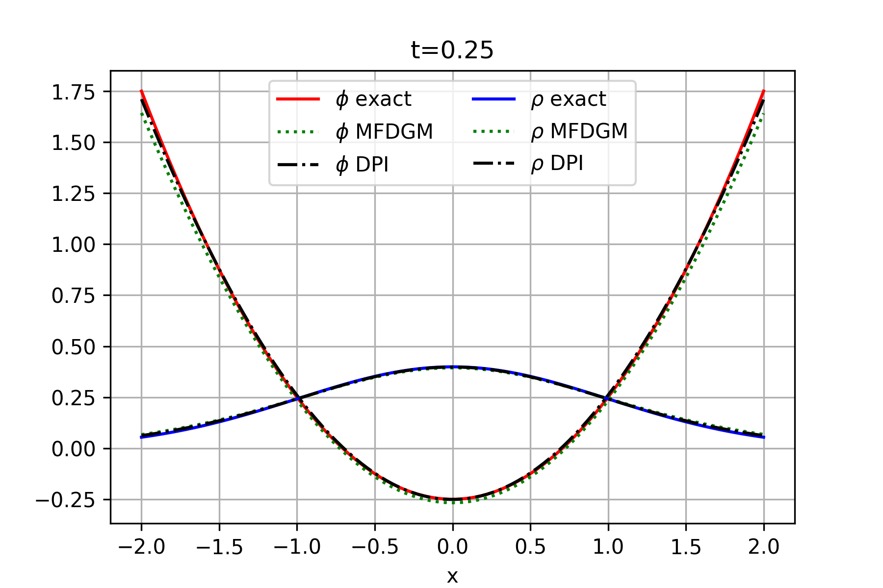
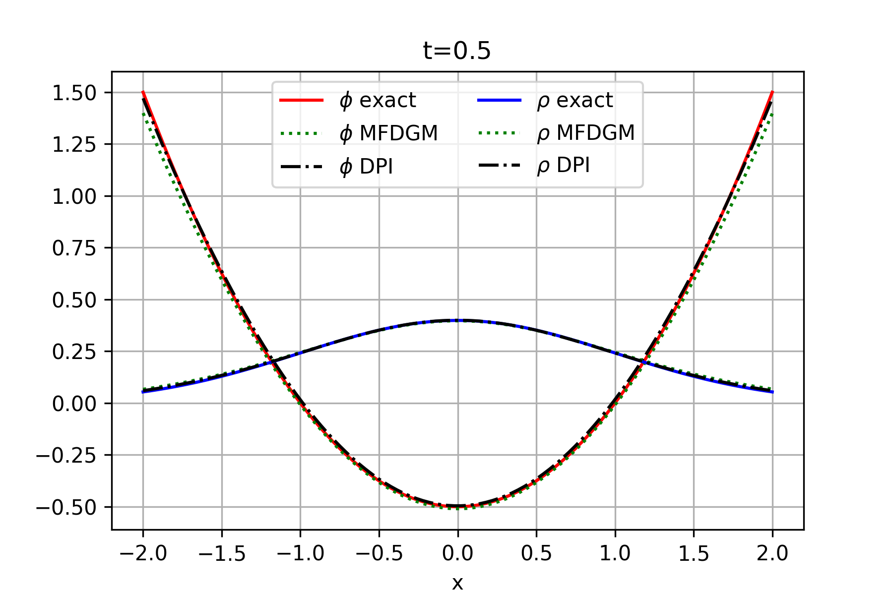
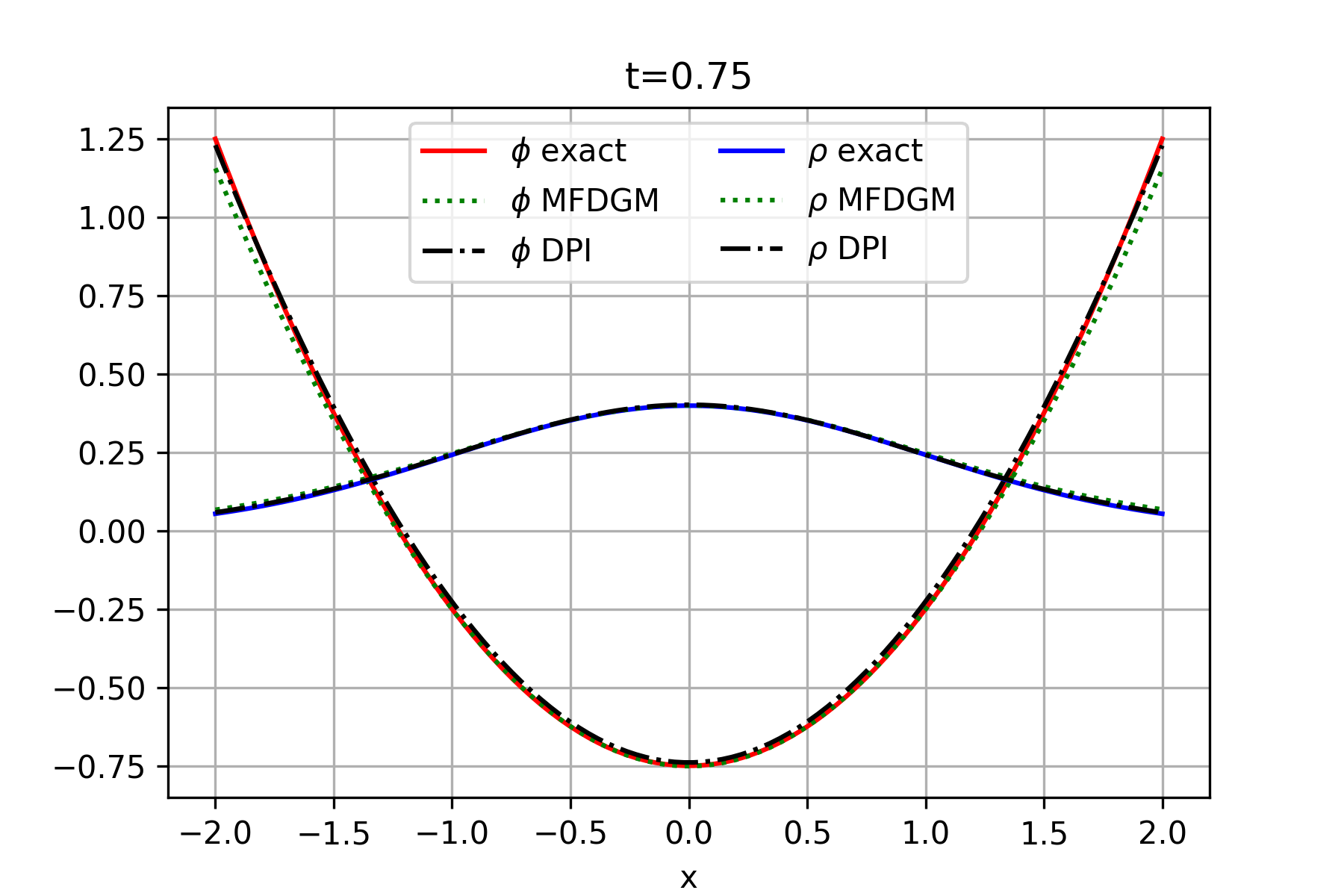
Figure 1: Comparison of Exact Solution and Prediction using DPI and MFDGM in one-Dimension at t=(0.25, 0.5, 0.75) with $\gamma=0$

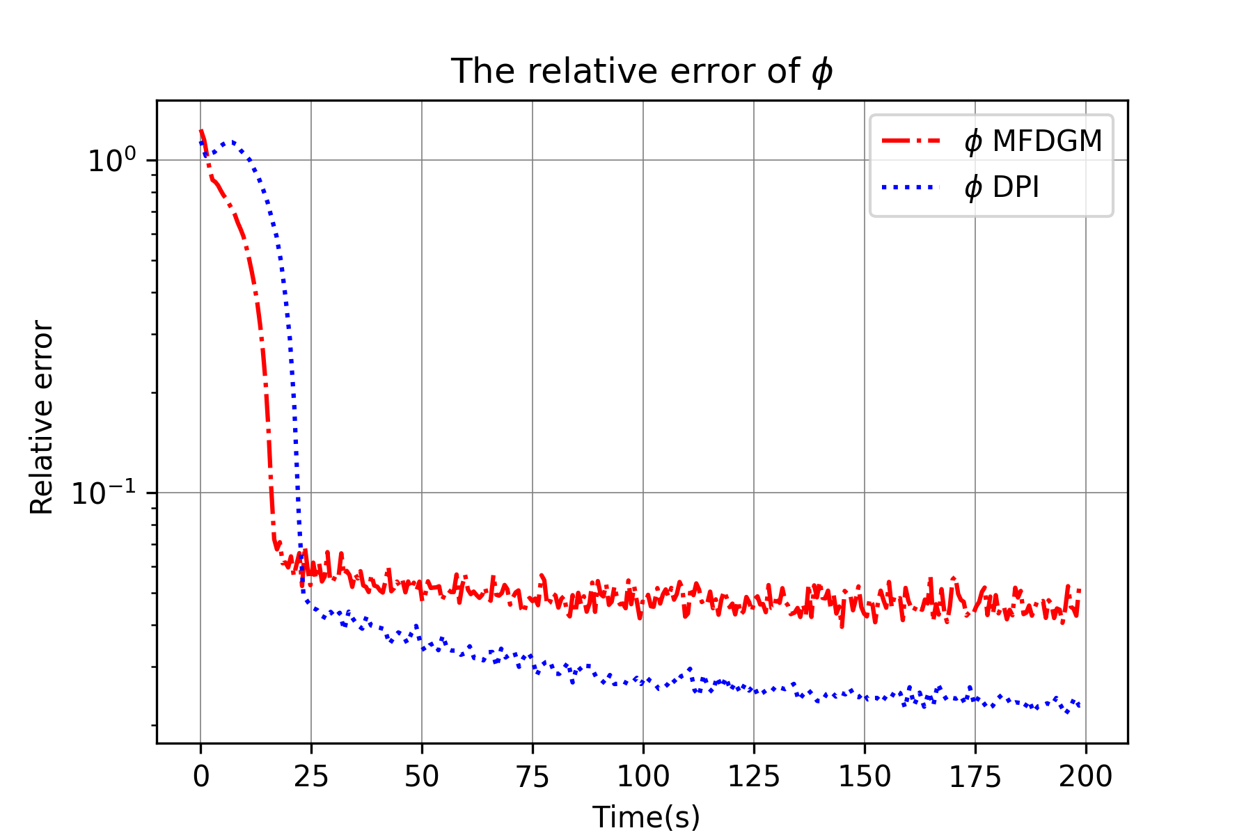
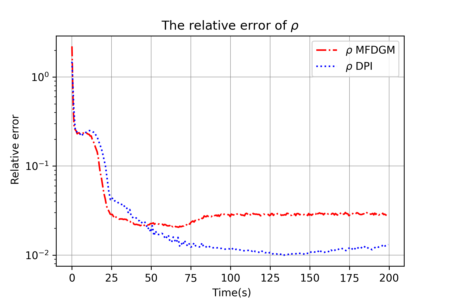
Figure 2: Comparison of Relative Error for $\phi$ and $\rho$ using Two Methods with $\gamma=0$.

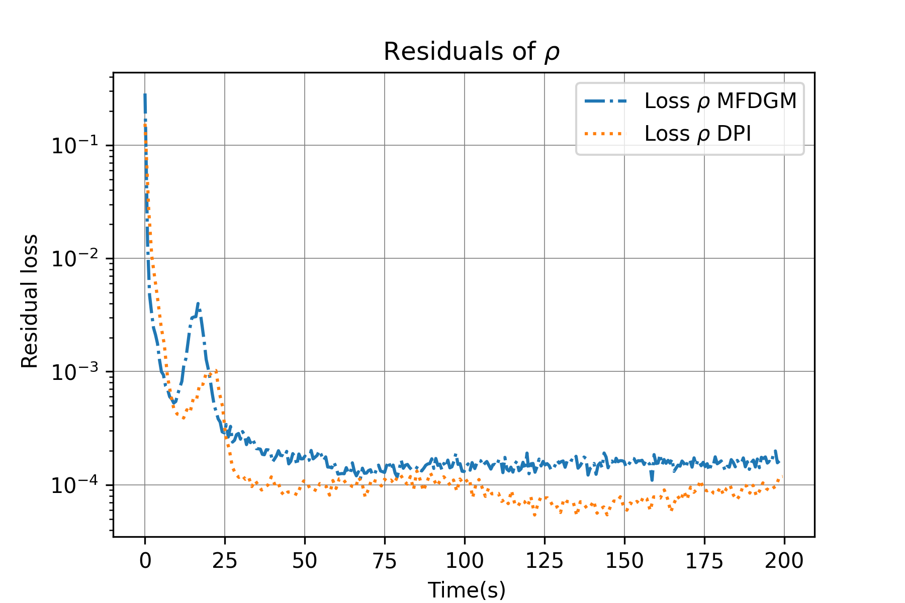
Figure 3: Comparison of losses for $\phi$ and $\rho$ using Two Methods with $\gamma=0$.

Test 2: In order to investigate the impact of congestion on the previous case, we repeat the same experiment with the same parameters, but this time we consider a non-zero congestion parameter $(\gamma=0.1)$. We present the numerical results in Figures 4, 5, 6.

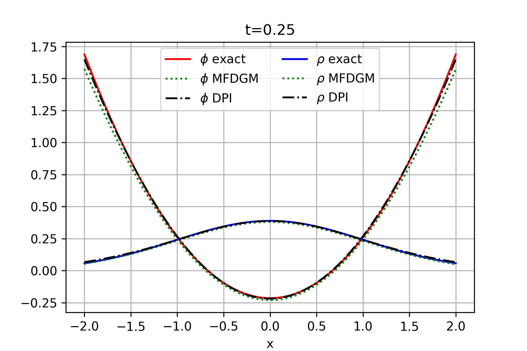
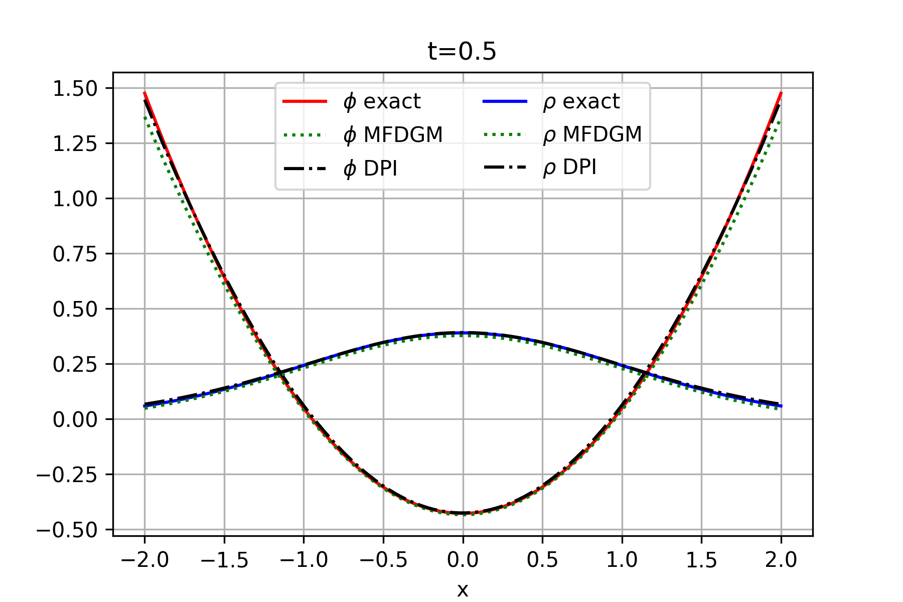
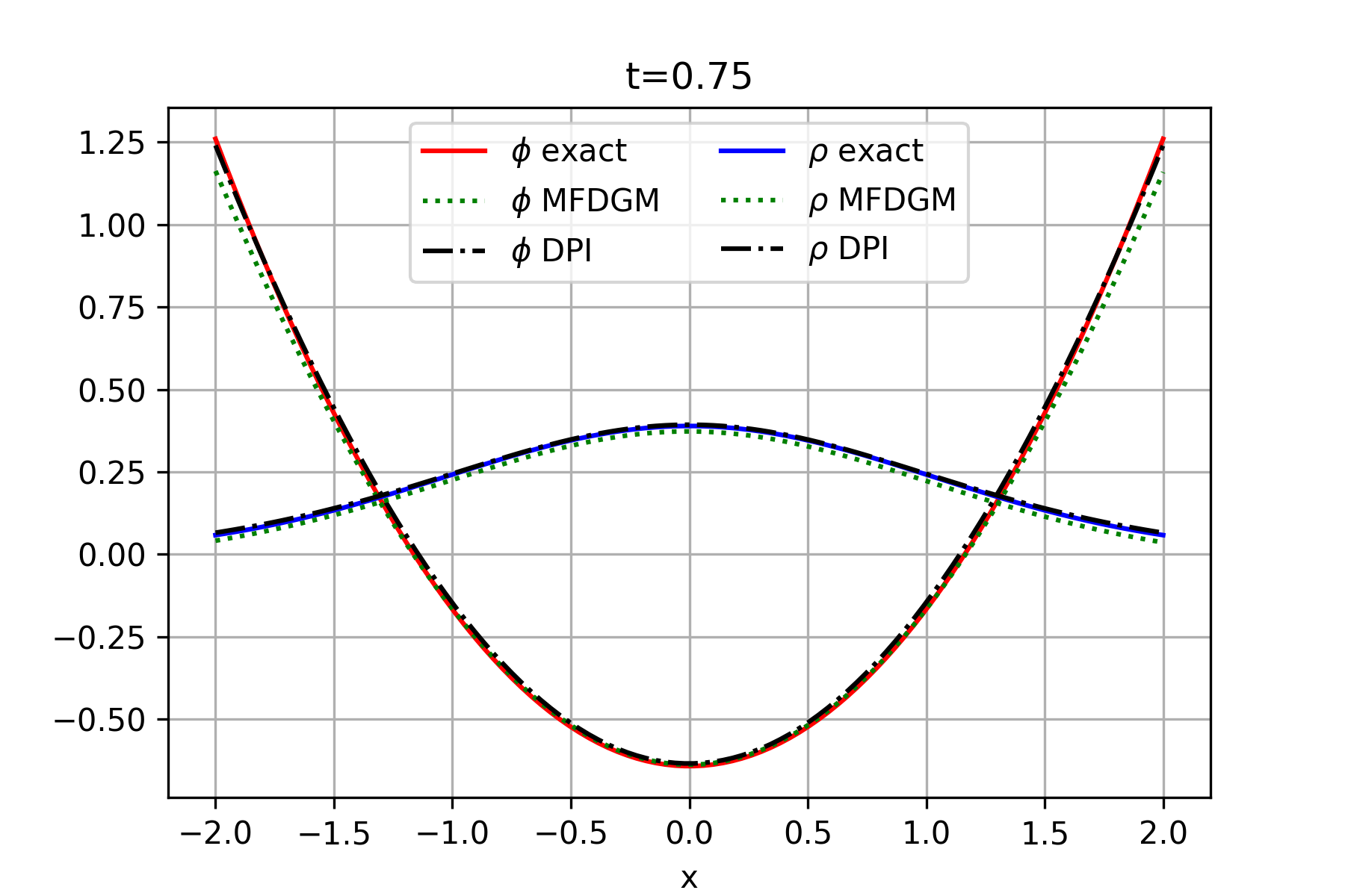
Figure 4: Comparison of Exact Solution and Prediction using DPI and MFDGM in One Dimension at t=(0.25, 0.5, 0.75) with $\gamma=0.1$

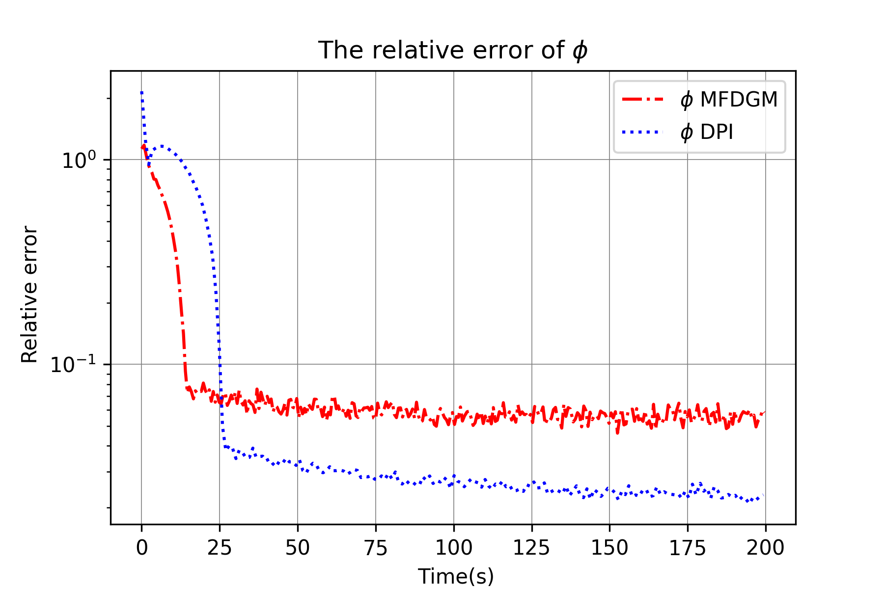
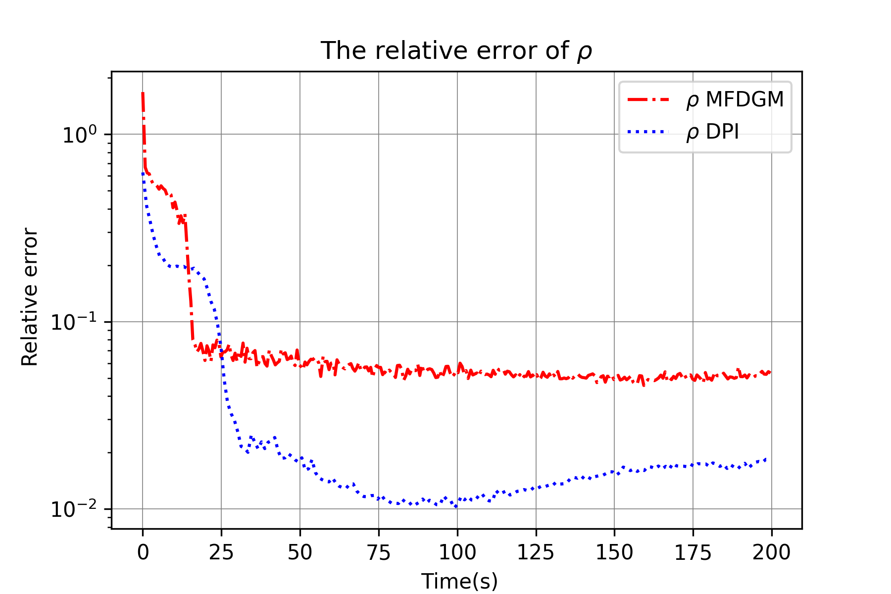
Figure 5: Comparison of Relative Error for $\phi$ and $\rho$ using Two Methods with $\gamma=0.1$.

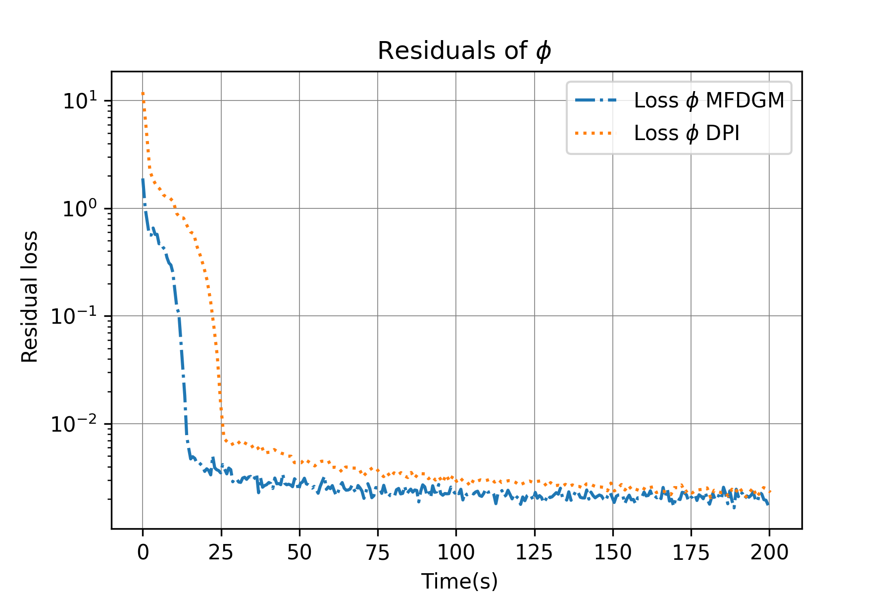
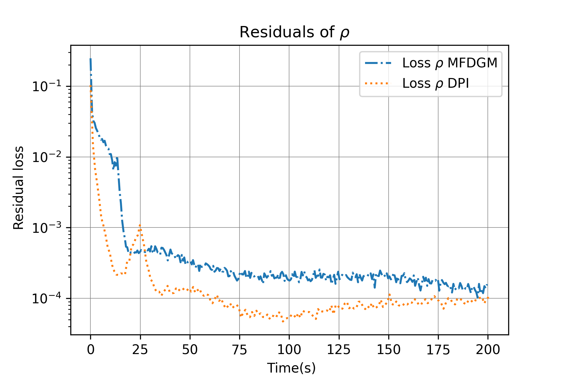
Figure 6: Comparison of losses for $\phi$ and $\rho$ using Two Methods with $\gamma=0.1$.

In comparison to the MFDGM algorithm, DPI demonstrates a higher level of effectiveness, particularly when applied to congestion scenarios. This superiority can be attributed to DPI’s ability to reduce the complexity of Partial Differential Equations (PDEs) through the incorporation of a policy neural network. Furthermore, to mitigate errors such as MFDGM, we enforce training DPI within the boundaries. This additional measure ensures improved accuracy in the training process. By leveraging this neural network, DPI offers a more suitable approach for handling congestion-related tests, surpassing the capabilities of the MFDGM algorithm.
Test 3: In this test, we aim to solve (11) using PI. To enable the application of this method, we incorporate periodic boundary conditions into (6). In their research, the authors utilized Policy Iteration methods to solve a Partial Differential Equation (PDE) system through finite-difference approximation. They adopted a uniform grid $\mathcal{G}$ and centred second-order finite differences for the discrete Laplacian while computing the Hamiltonian and divergence term in the FP equation using the Engquist-Osher numerical flux for conservation laws. The symbol $\sharp$ represented the linear differential operators at the grid nodes. Specifically, in the context of one dimension, they implemented a uniform discretization of $E$ with $I$ nodes $x_{i}=ih$, where $h=1/I$ is the space step. To discretize time, they employed an implicit Euler method for both the time-forward FP equation and the time-backward HJB equation, with a uniform grid on the interval $[0,T]$ with $N+1$ nodes $t_{n}=nt$, where $t=T/N$ was the time step. To prevent any confusion, we adhere to the previously established notation. Therefore, we use $\phi$, $\rho$, and the policy $q$ to represent the vectors that approximate the solution on $\mathcal{G}$, and by $\phi_{n},\rho_{n},$ and $q_{n}$ the vectors on $\mathcal{G}$ approximating the solution and policy at time $t_{n}$. The algorithm we will use for the fully discretized System 11 is as follows: we start with an initial guess $q^{(0)}_{n}:\mathcal{G}\to\mathbb{R}^{2d}$ for $n=0,...,N,$ and initial and final data $\rho_{0},\phi_{N}:\mathcal{G}\to\mathbb{R}$. We then iterate on $k\geq 0$ until convergence,
(i) Solve for $n=0,\ldots,N-1$ on $\mathcal{G}$

$$\left\{\begin{array}[]{l}\rho_{n+1}^{(k)}-dt\left(\Delta_{\sharp}\rho_{n+1}^{(k)}+\operatorname{div}_{\sharp}\left(\rho_{n+1}^{(k)}q_{n+1}^{(k)}\right)\right)=\rho_{n}^{(k)}\\ \rho_{0}^{(k)}=\rho_{0}\end{array}\right.$$

(ii) Solve for $n=N-1,\ldots,0$ on $\mathcal{G}$

$$\left\{\begin{aligned} \phi_{n}^{(k)}&-dt\left(\Delta_{\sharp}\phi_{n}^{(k)}-q_{n,\pm}^{(k)}\cdot D_{\sharp}\phi_{n}^{(k)}\right)\\ &=\phi_{n+1}+dt\left(\frac{1}{2}\left|q_{n+1,\pm}^{(k)}\right|^{2}+x_{i}^{2}+\gamma Ln\left(\rho_{n+1}^{(k)}\right)\right)\\ \phi_{N}^{(k)}&=\phi_{N}\end{aligned}\right.$$

(iii) Update the policy $q_{n}^{(k+1)}=D_{\sharp}\phi_{n}^{(k)}$ on $\mathcal{G}$ for $n=0,\ldots,N$, and set $k\leftarrow$ $k+1$. In the following test, we choose $\gamma=0$, T = 1 for the final time, and $K=50$. The grid consisted of $I=200$ nodes in space and $N=200$ nodes in time. The initial policy was initialized as $q^{(0)}_{n}\equiv(0,0)$ on $\mathcal{G}$ for all $n$.

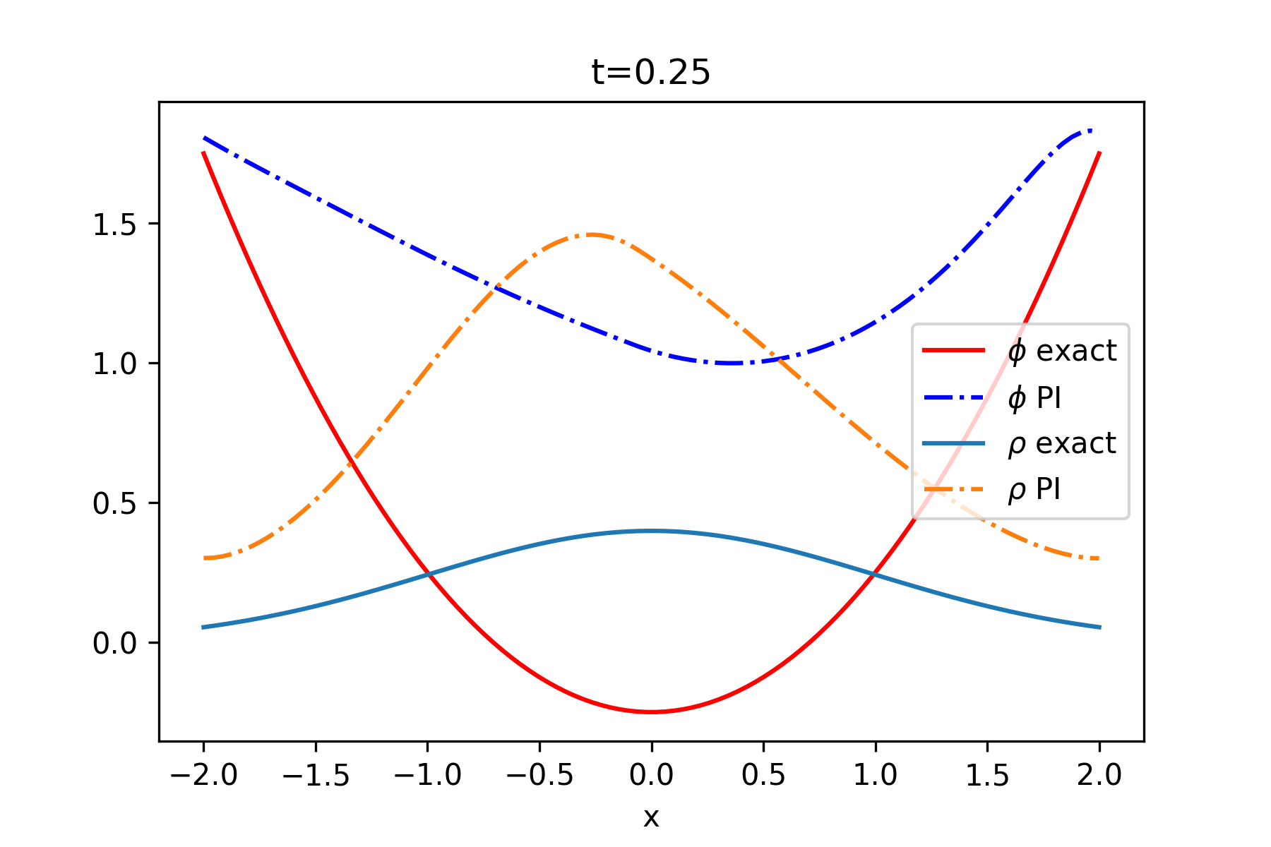
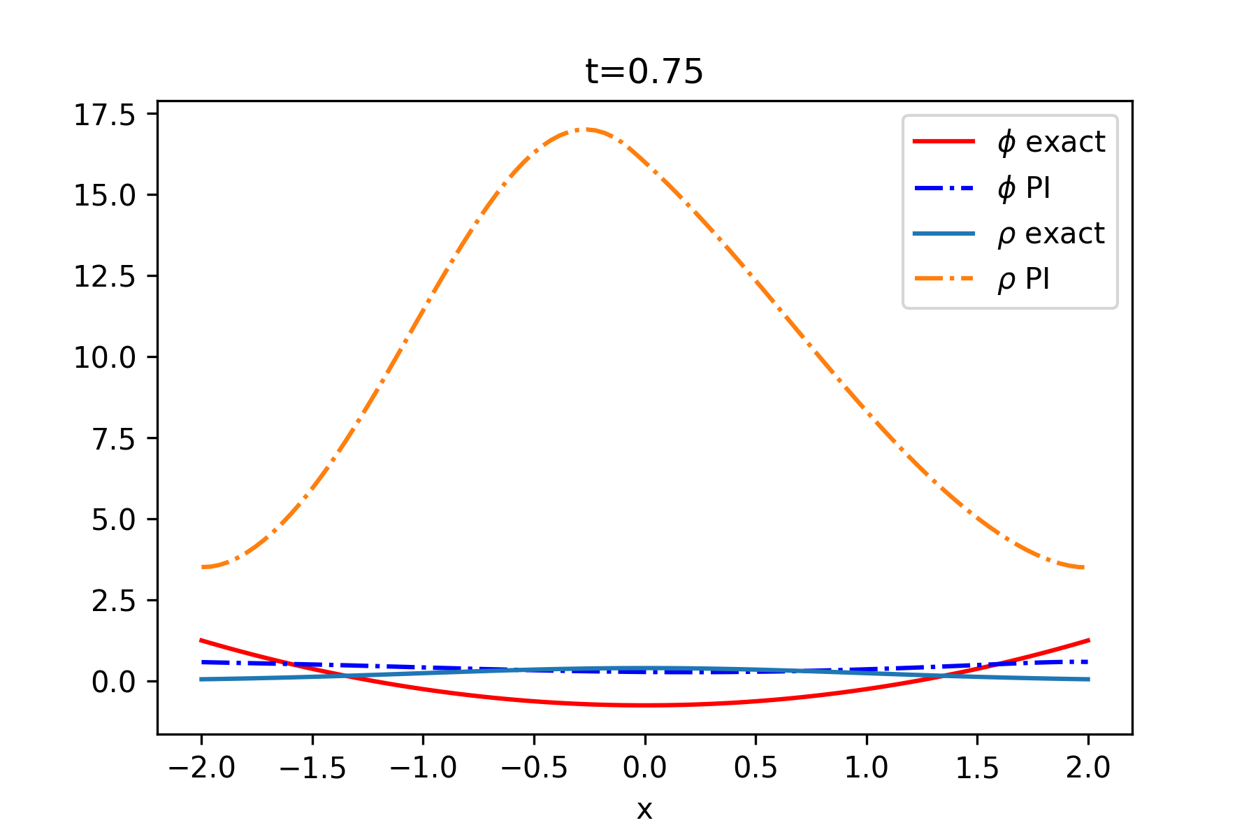
Figure 7: Comparison of Exact Solution and Prediction using PI in One Dimension at t=(0.25, 0.5, 0.75) with $\gamma=0$

The results of the study Figure 7 showed that policy iteration is not effective in solving MFG problems in separable cases. However, the use of deep learning instead of finite difference methods has exhibited promise in extending the applicability of this approach to MFG in the separable case. In future examinations, we will conduct a thorough assessment to explore the potential of DPI in addressing more intricate MFG problems.

Test 4: The effectiveness of our approach in high-dimensional cases is tested in this experiment and the next section. We solve the MFG system (11) for dimensions 2, 50, and 100 and present the results in Figure 8. To train the neural networks, we use a minibatch of 100, 500, and 1000 samples respectively for d=2, 50 and 100. The neural networks have a single hidden layer consisting of 100, 200 and 256 neurons each respectively. We utilize the Softplus activation function for $N_{\omega}$ and the Tanh activation function for $N_{\tau}$ and $N_{\theta}$. We use ADAM with a learning rate of $10^{-4}$, weight decay of $10^{-4}$, and employ ResNet as the architecture with a skip connection weight of 0.5. The results were obtained after applying a Savgol filter to enhance the clarity of the curves

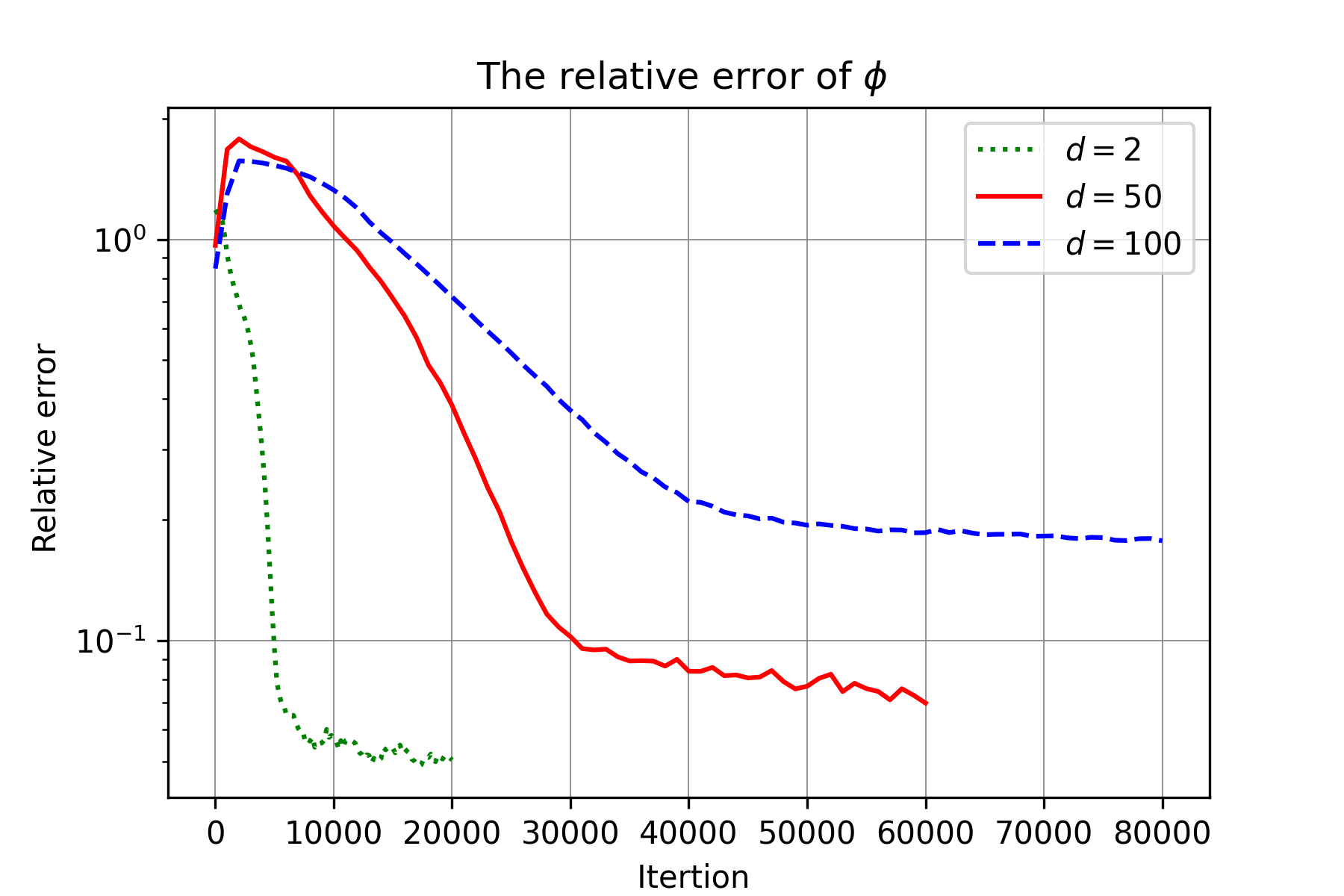
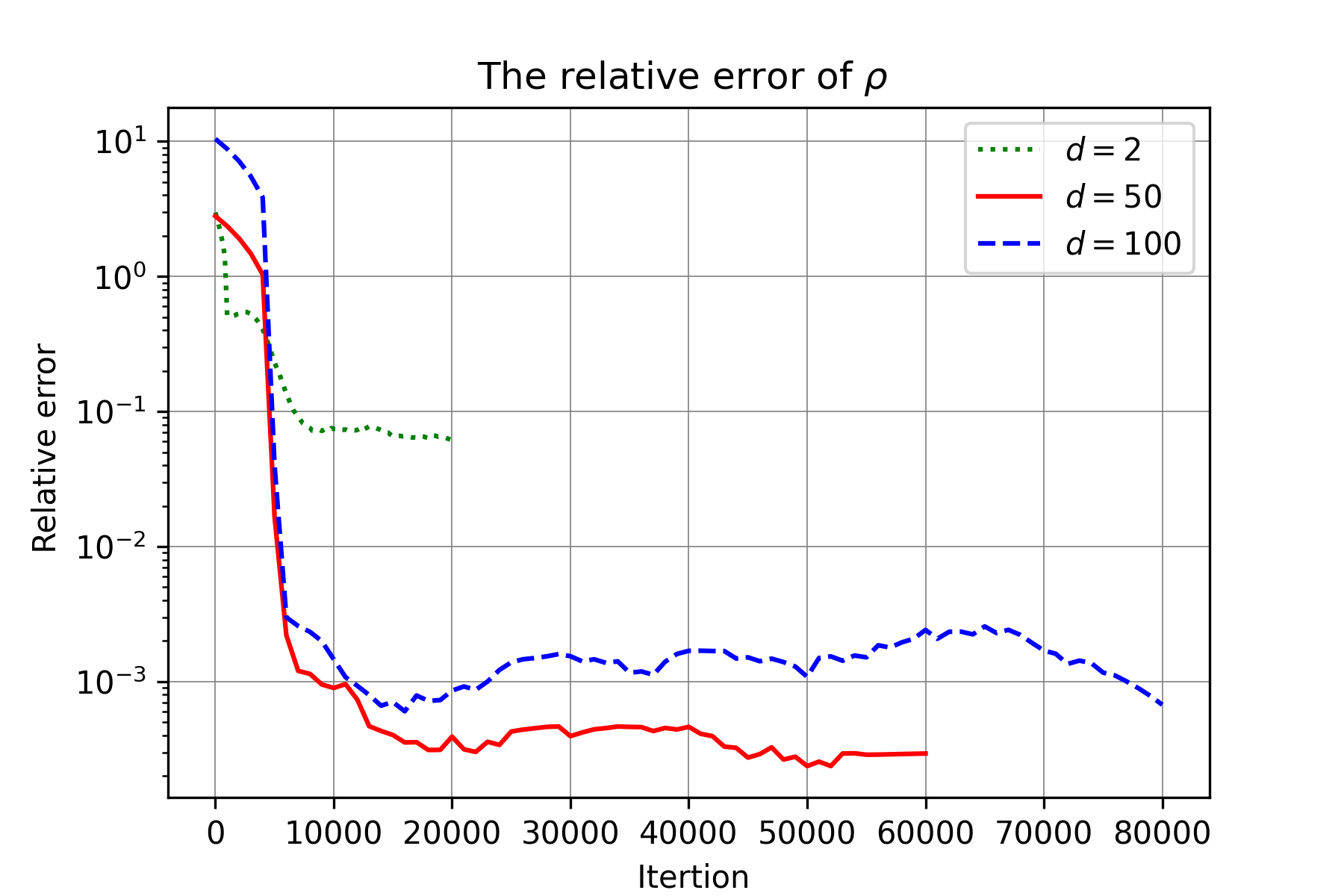
Figure 8: The relative Error for $\phi$ and $\rho$ DPI Method for d=2, 50 and 100

4.2 High-Dimensional

In this section, our goal is to further assess the effectiveness of our approach in high-dimensional contexts by examining two specific examples characterized by non-separable Hamiltonians, as previously introduced in [3].

Example 1: We consider the following problem in the stochastic case with $\nu=0.3$. The problem is defined within the domain $\Omega=[0,1]^{d}$, with a fixed final time of $T=1$. In this context, the terminal cost is specified as $g=0,$ and the initial density is characterized by a Gaussian distribution.
The corresponding MFG system is,

$$\left\{\begin{array}[]{rrrrr}-\phi_{t}-\nu\Delta\phi+\frac{1}{2(1+4\rho)}||\phi_{x}||^{2}=0,\\ \rho_{t}-\nu\Delta\rho-\operatorname{div}(\rho\frac{\phi_{x}}{1+4\rho})=0,\\ \rho(0,x)=\left(\frac{1}{2\pi}\right)^{d/2}e^{-\frac{||x-0.25||^{2}}{2}},\\ \phi(x,T)=0.\end{array}\right.\vspace{-0.25cm}$$ (13)

We addressed the MFG system (13) across three different dimensions: 2, 10, and 50. The results of this analysis are presented in Figure 9. For the training of neural networks, we adopted varying minibatch sizes: 100, 500, and 1000 samples, corresponding to $d=2,10$, and $100$. These neural networks consist of a single hidden layer with 100. We applied the Softplus activation function for $N_{\omega}$ and the Tanh activation function for $N_{\tau}$ and $N_{\theta}$. Our optimization approach used ADAM with a learning rate of $10^{-4}$ and a weight decay of $10^{-4}$. We employed the ResNet architecture with a skip connection weight of 0.5. To enhance the smoothness of the curves, the results underwent a Savgol filter.

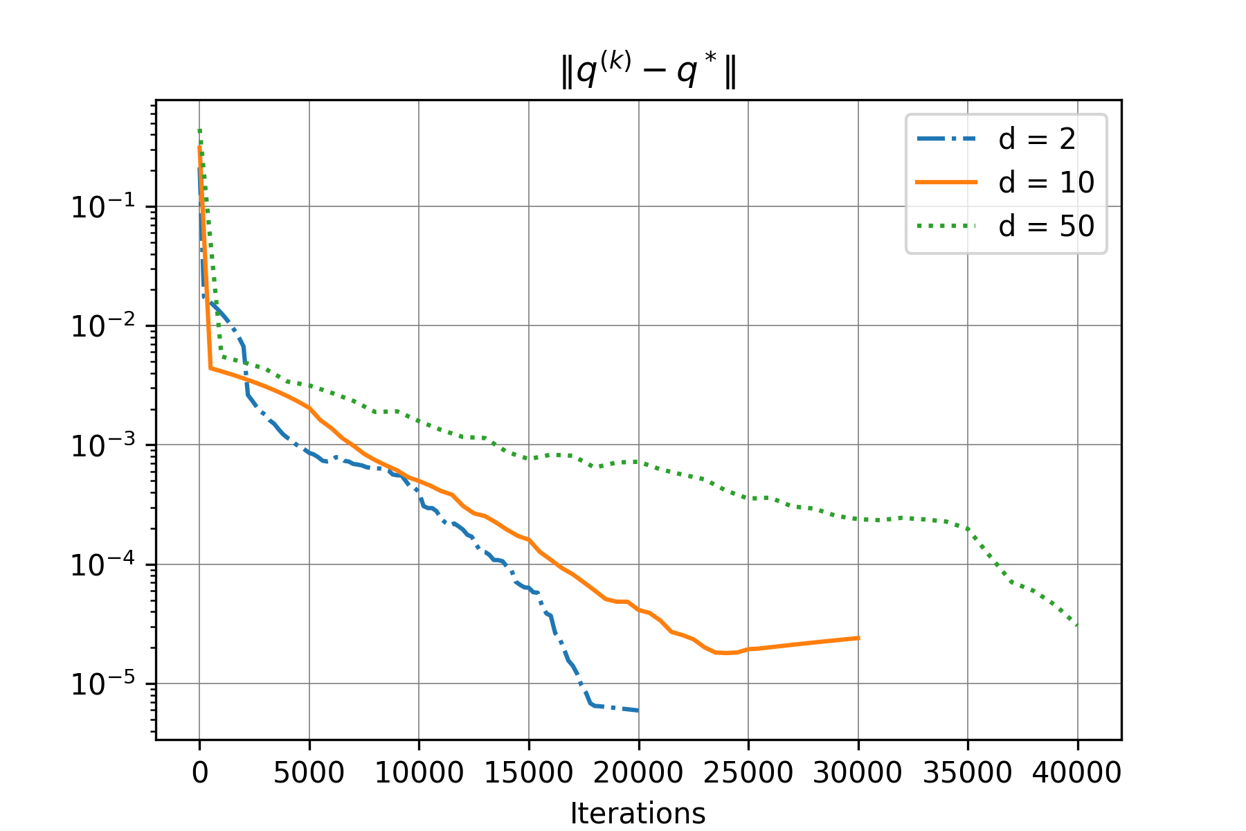
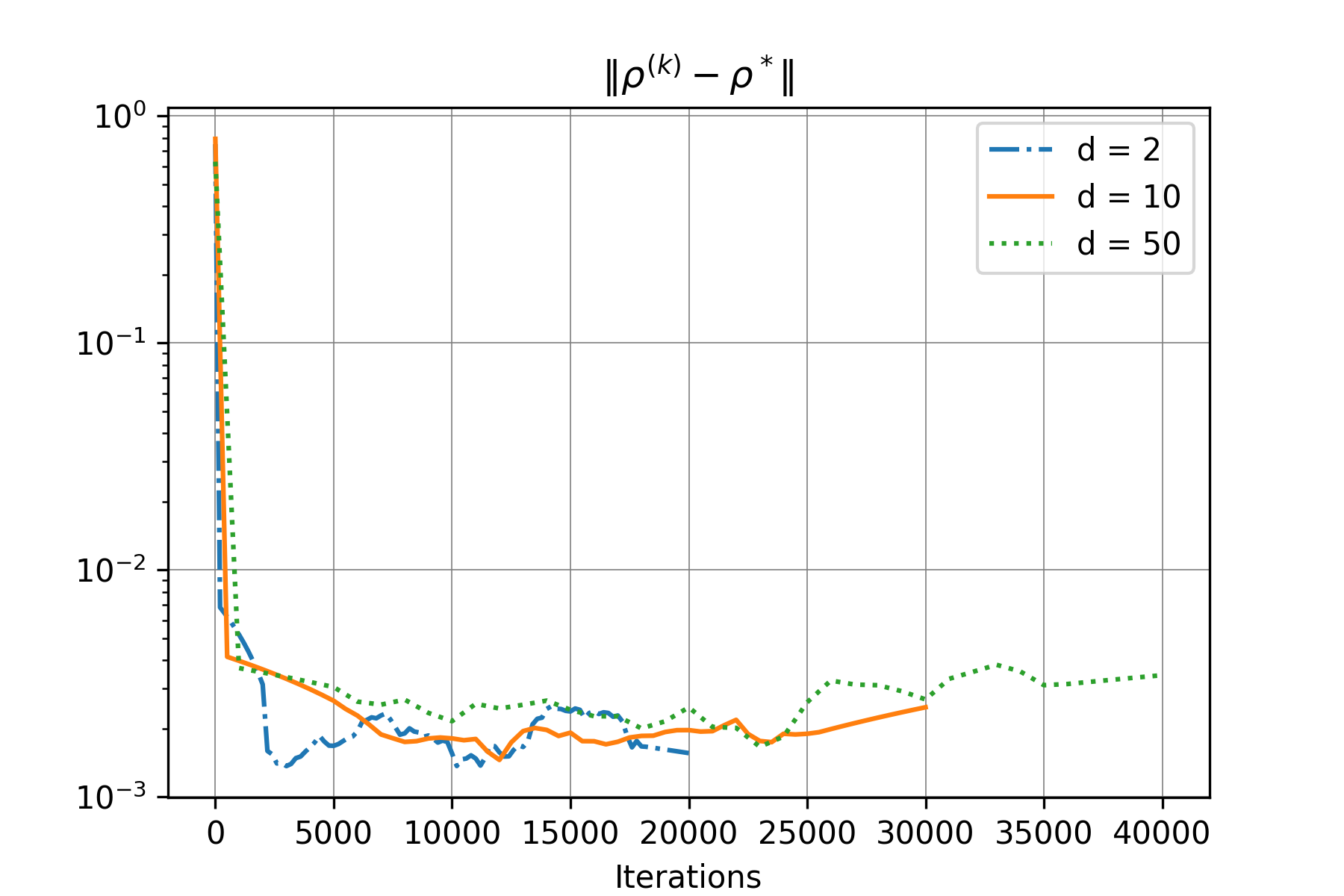
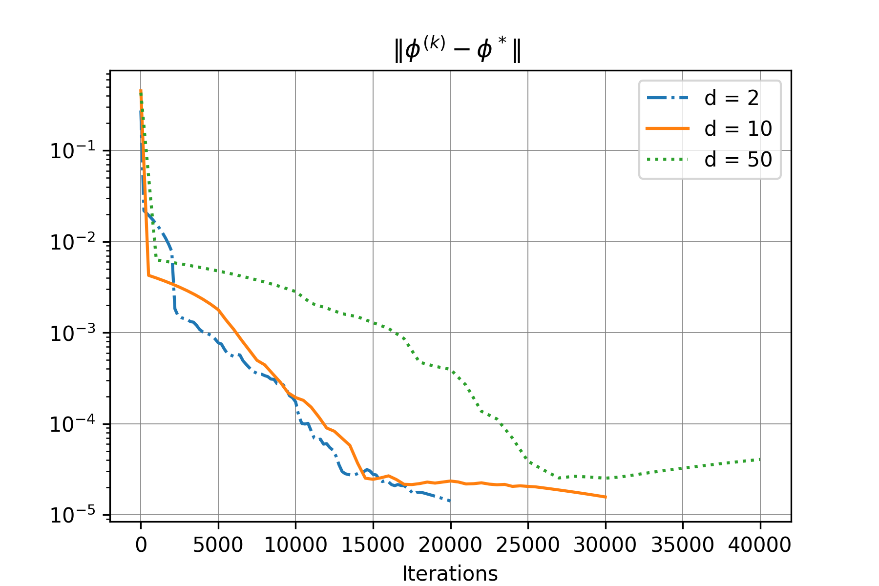
Figure 9: Example1: The $L^{\infty}$ Distance between $\rho^{(k)}$, $\phi^{(k)}$ and $q^{(k)}$ from DPI and the final solution $\rho^{*}$, $\phi^{*}$ and $q^{*}$ for d=2, 10 and 50.

Example 2: Now we give the following problem with a terminal cost that motivates the agents to direct their movements toward particular sub-regions within the domain.
The corresponding MFG system is,

$$\left\{\begin{array}[]{rrrrr}-\phi_{t}-\nu\Delta\phi+\frac{1}{2\rho^{1/2}}||\phi_{x}||^{2}=0,\\ \rho_{t}-\nu\Delta\rho-\operatorname{div}(\rho\frac{\phi_{x}}{\rho^{1/2}})=0,\\ \rho(0,x)=\left(\frac{1}{2\pi}\right)^{d/2}e^{-\frac{||x-0.25||^{2}}{2}},\\ \phi(x,T)=\sum_{i=1}^{d}cos(2\pi x_{i}).\end{array}\right.\vspace{-0.25cm}$$ (14)

We perform the same process as previously described in Example 1 for the MFG system (14), and the results of this analysis are presented in Figure 10.

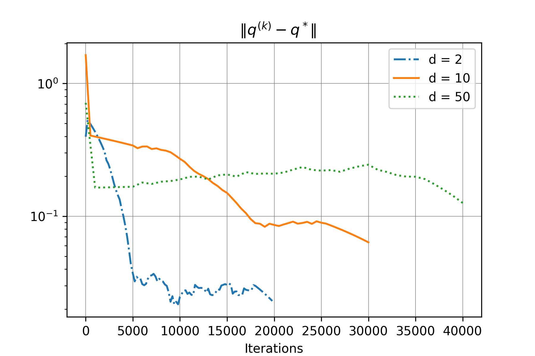
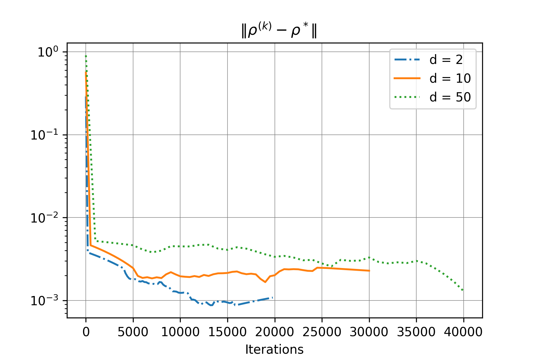
Figure 10: Example2: The $L^{\infty}$ Distance between $\rho^{(k)}$, $\phi^{(k)}$ and $q^{(k)}$ from DPI and the final solution $\rho^{*}$, $\phi^{*}$ and $q^{*}$ for d=2, 10 and 50.

4.3 Trafic Flow

To assess the DPI method, we conducted experiments on a traffic flow problem for an autonomous vehicle used to test the effectiveness of MFDGM. We specifically chose this problem because it is characterized by a non-separable Hamiltonian, making it a more complex and challenging problem. In our experiments, we applied the PI and DPI Methods to the problem and evaluated its performance in stochastic cases $\nu=0.1$. We consider the traffic flow problem on the spatial domain $\Omega=[0,1]$ with dimension $d=1$ and final time $T=1$. The terminal cost $g$ is set to zero and the initial density $\rho_{0}$ is given by a Gaussian distribution, $\rho_{0}(x)=0.05-0.9\exp\left(\frac{-1}{2}\left(\frac{x-0.5}{0.1}\right)^{2}\right)$.
The corresponding MFG system is,

$$\left\{\begin{array}[]{rrrrr}\phi_{t}+\nu\Delta\phi-\frac{1}{2}||\phi_{x}||^{2}+(1-\rho)\phi_{x}=0\\ \rho_{t}-\nu\Delta\rho-\operatorname{div}((\phi_{x}-(1-\rho))\rho)=0\\ \rho(x,0)=0.05-0.9\exp(\frac{-1}{2}(\frac{x-0.5}{0.1})^{2}),\\ \phi(x,T)=0.\end{array}\right.\vspace{-0.25cm}$$ (15)

Test 1: In this test, we aim to solve (15) with periodic boundary conditions, we utilized Algorithm 1 with a minibatch size of 50 samples at each iteration to obtain results. Our approach involved the use of neural networks with different hidden layers, each consisting of 100 neurons. Specifically, for $N_{\theta}$, we employed three hidden layers with the Gelu activation function, while for $N_{\omega}$ and $N_{\tau}$, we used a single hidden layer with the Sin activation function. During the training process, we employed the ADAM optimizer with a learning rate of $10^{-4}$ and weight decay of $10^{-3}$. To construct the neural networks, we adopted the ResNet architecture, incorporating a skip connection weight of 0.5.
To assess the performance of the methods, we conducted an analysis of the numerical results presented in Figure 11. This figure provides visual representations of the density solution as well as the $L^{\infty}$ Distance between $\rho^{(k)}$, $\phi^{(k)}$ and $q^{(k)}$ from DPI and the final solution $\rho^{*}$, $\phi^{*}$ and $q^{*}$ from fixed point algorithm. The $L^{\infty}$ Distance values were obtained after applying a Savgol filter to enhance the clarity of the curves.

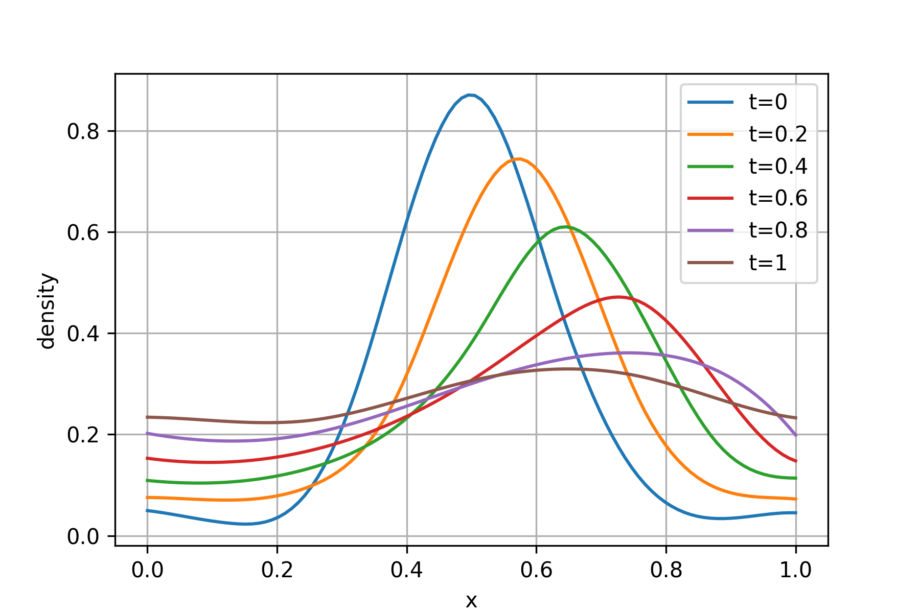
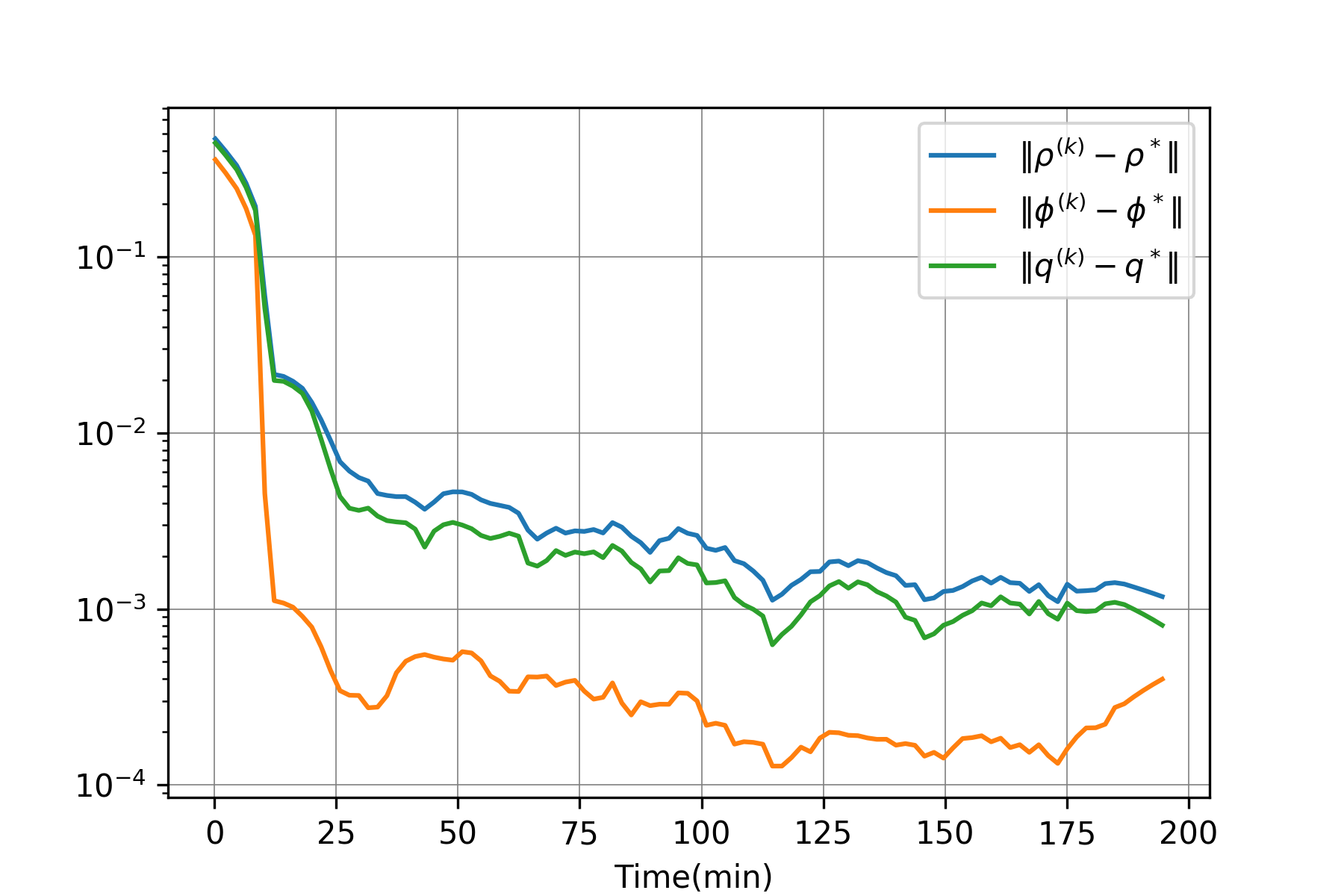
Figure 11: the density solution obtained with DPI and $L^{\infty}$ Distance between $\rho^{(k)}$, $\phi^{(k)}$ and $q^{(k)}$ from DPI and the final solution $\rho^{*}$, $\phi^{*}$ and $q^{*}$ from fixed point algorithm

Test 2: The purpose of this test is to utilize the PI method in order to solve (15) with periodic boundary conditions. Similar to Test 3, we employ PI algorithm to solve the fully discretized (15) as follows: we start with an initial guess $q^{(0)}_{n}:\mathcal{G}\to\mathbb{R}^{2d}$ for $n=0,...,N,$ and initial and final data $\rho_{0},\phi_{N}:\mathcal{G}\to\mathbb{R}$. We then iterate on $k\geq 0$ until convergence:
(i) Solve for $n=0,\ldots,N-1$ on $\mathcal{G}$

$$\left\{\begin{array}[]{l}\rho_{n+1}^{(k)}-dt\left(\Delta_{\sharp}\rho_{n+1}^{(k)}+\operatorname{div}_{\sharp}\left(\rho_{n+1}^{(k)}q_{n+1}^{(k)}\right)\right)=\rho_{n}^{(k)}\\ \rho_{0}^{(k)}=\rho_{0}\end{array}\right.$$

(ii) Solve for $n=N-1,\ldots,0$ on $\mathcal{G}$

$$\left\{\begin{aligned} \phi_{n}^{(k)}&-dt\left(\Delta_{\sharp}\phi_{n}^{(k)}-q_{n,\pm}^{(k)}\cdot D_{\sharp}\phi_{n}^{(k)}\right)\\ &=\phi_{n+1}+\frac{dt}{2}\left(\left|q_{n+1,\pm}^{(k)}\right|^{2}+\left|1-\rho_{n+1}^{(k)}\right|^{2}+\left(1-\rho_{n+1}^{(k)}\right)q_{n+1,\pm}^{(k)}\right)\\ \phi_{N}^{(k)}&=\phi_{N}\end{aligned}\right.$$

(iii) Update the policy $q_{n}^{(k+1)}=D_{\sharp}\phi_{n}^{(k)}$ on $\mathcal{G}$ for $n=0,\ldots,N$, and set $k\leftarrow$ $k+1$. In the following test, we choose $\gamma=0$, T = 1 for the final time, and $K=50$. The grid consisted of $I=200$ nodes in space and $N=200$ nodes in time. The initial policy was initialized as $q^{(0)}_{n}\equiv(0,0)$ on $\mathcal{G}$ for all $n$. Figure 12 presents the numerical results, offering visual depictions of both the density solution and the $L^{\infty}$ Distance between $\rho^{(k)}$, $\phi^{(k)}$ and $q^{(k)}$ from policy iteration and the final solution $\rho^{*}$, $\phi^{*}$ and $q^{*}$ from fixed point algorithm.

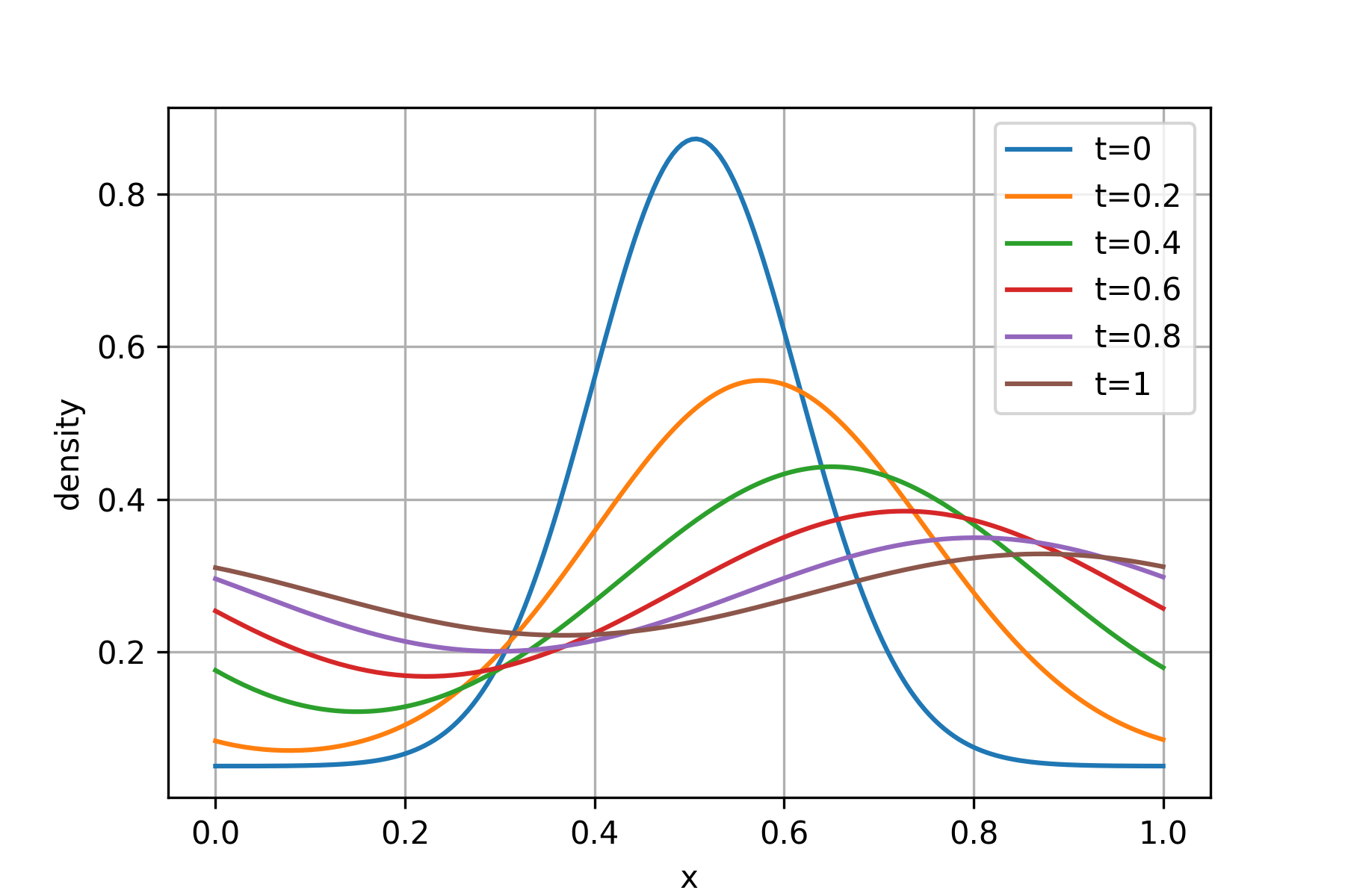
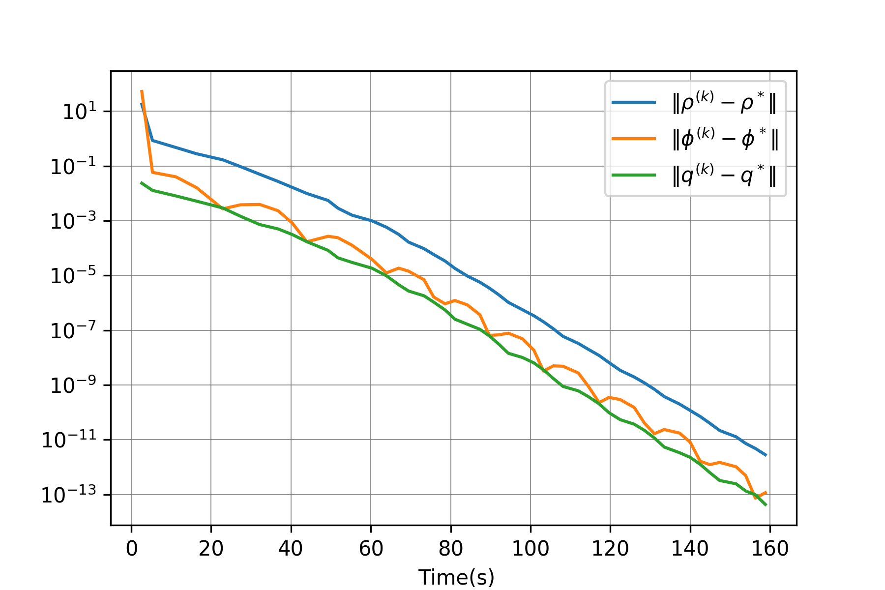
Figure 12: the density solution obtained with policy iteration and $L^{\infty}$ Distance between $\rho^{(k)}$, $\phi^{(k)}$ and $q^{(k)}$ from policy iteration and the final solution $\rho^{*}$, $\phi^{*}$ and $q^{*}$ from fixed point algorithm

The findings of this study revealed that policy iteration outperforms deep policy iteration in terms of effectiveness and speed. Consequently, we can deduce that traditional methods are commonly employed to address such problems. However, it is important to note that traditional methods have limitations, such as the curse of dimensionality. Hence, there is a growing interest in utilizing deep learning approaches as an alternative solution.

5 Conclusion

We have presented a novel approach that combines the MFDGM method and the PI method to tackle high-dimensional stochastic MFG. Our approach exhibits a higher level of effectiveness, particularly in congestion scenarios, compared to the MFDGM algorithm. Additionally, we have observed that while our DPI approach demonstrates effectiveness for general MFG, the traditional PI method outperforms DPI in terms of effectiveness and speed when dealing with non-separable Hamiltonians. It can be deduced that traditional methods are commonly employed to address such problems in low-dimensional settings, but DPI extends its capabilities to high-dimensional scenarios.

References

- [1] M. Assouli, B. Missaoui, Deep learning for mean field games with non-separable hamiltonians, Chaos, Solitons & Fractals 174 (2023) 113802. doi:https://doi.org/10.1016/j.chaos.2023.113802.
- [2] S. Cacace, F. Camilli, A. Goffi, A policy iteration method for mean field games, ESAIM: Control, Optimisation and Calculus of Variations 27 (2021) 85.
- [3] M. Lauriére, J. Song, Q. Tang, Policy iteration method for time-dependent mean field games systems with non-separable hamiltonians, arXiv preprint arXiv:2110.02552 (2021).
- [4] J.-M. Lasry, P.-L. Lions, Mean field games, Japanese journal of mathematics 2 (1) (2007) 229–260.
- [5] K. Huang, X. Di, Q. Du, X. Chen, A game-theoretic framework for autonomous vehicles velocity control: Bridging microscopic differential games and macroscopic mean field games, arXiv preprint arXiv:1903.06053 (2019).
- [6] H. Shiri, J. Park, M. Bennis, Massive autonomous uav path planning: A neural network based mean-field game theoretic approach, in: 2019 IEEE Global Communications Conference (GLOBECOM), IEEE, 2019, pp. 1–6.
- [7] P. Cardaliaguet, C.-A. Lehalle, Mean field game of controls and an application to trade crowding, Mathematics and Financial Economics 12 (3) (2018) 335–363.
- [8] P. Casgrain, S. Jaimungal, Algorithmic trading in competitive markets with mean field games, SIAM News 52 (2) (2019) 1–2.
- [9] Y. Achdou, J. Han, J.-M. Lasry, P.-L. Lions, B. Moll, Income and wealth distribution in macroeconomics: A continuous-time approach, Tech. rep., National Bureau of Economic Research (2017).
- [10] Y. Achdou, F. J. Buera, J.-M. Lasry, P.-L. Lions, B. Moll, Partial differential equation models in macroeconomics, Philosophical Transactions of the Royal Society A: Mathematical, Physical and Engineering Sciences 372 (2028) (2014) 20130397.
- [11] D. A. Gomes, L. Nurbekyan, E. Pimentel, Economic models and mean-field games theory, Publicaoes Matematicas, IMPA, Rio, Brazil (2015).
- [12] A. T. Lin, S. W. Fung, W. Li, L. Nurbekyan, S. J. Osher, Apac-net: Alternating the population and agent control via two neural networks to solve high-dimensional stochastic mean field games, arXiv preprint arXiv:2002.10113 (2020).
- [13] J.-M. Lasry, P.-L. Lions, Jeux à champ moyen. ii–horizon fini et contrôle optimal, Comptes Rendus Mathématique 343 (10) (2006) 679–684.
- [14] Y. Achdou, A. Porretta, Mean field games with congestion, Annales de l’Institut Henri Poincare (C) Non Linear Analysis 35 (06 2017). doi:10.1016/j.anihpc.2017.06.001.
- [15] D. A. Gomes, V. K. Voskanyan, Short-time existence of solutions for mean-field games with congestion, Journal of the London Mathematical Society 92 (3) (2015) 778–799.
- [16] Y. Achdou, P. Cardaliaguet, F. Delarue, A. Porretta, F. Santambrogio, Y. Achdou, M. Laurière, Mean field games and applications: Numerical aspects, Mean Field Games: Cetraro, Italy 2019 (2020) 249–307.
- [17] P. Hammer, Adaptive control processes: a guided tour (r. bellman) (1962).
-
[18]
R. Bellman,
Dynamic
programming, Science 153 (3731) (1966) 34–37.
arXiv:https://www.science.org/doi/pdf/10.1126/science.153.3731.34,
doi:10.1126/science.153.3731.34.
URL https://www.science.org/doi/abs/10.1126/science.153.3731.34 - [19] H. Cao, X. Guo, M. Laurière, Connecting gans, mfgs, and ot, arXiv preprint arXiv:2002.04112 (2020).
- [20] J. Sirignano, K. Spiliopoulos, Dgm: A deep learning algorithm for solving partial differential equations, Journal of computational physics 375 (2018) 1339–1364.
- [21] M. Raissi, Deep hidden physics models: Deep learning of nonlinear partial differential equations, The Journal of Machine Learning Research 19 (1) (2018) 932–955.