Matrix-product-state-based band-Lanczos solver for quantum cluster approaches

Abstract

We present a matrix-product state (MPS) based band-Lanczos method as solver for quantum cluster methods such as the variational cluster approximation (VCA). While a naïve implementation of MPS as cluster solver would barely improve its range of applicability, we show that our approach makes it possible to treat cluster geometries well beyond the reach of exact diagonalization methods. The key modifications we introduce are a continuous energy truncation combined with a convergence criterion that is more robust against approximation errors introduced by the MPS representation and provides a bound to deviations in the resulting Green’s function. The potential of the resulting cluster solver is demonstrated by computing the self-energy functional for the single-band Hubbard model at half filling in the strongly correlated regime, on different cluster geometries. Here, we find that only when treating large cluster sizes, observables can be extrapolated to the thermodynamic limit, which we demonstrate at the example of the staggered magnetization. Treating clusters sizes with up to $6\times 6$ sites we obtain excellent agreement with quantum Monte-Carlo results.

I Introduction

Exploring the quantum states of matter of two-dimensional strongly correlated electron systems is inherently difficult. Prime examples are the cuprate high-temperature superconductors Bednorz and Müller (1986), whose salient features are frequently described within a single-band Hubbard-type model on a square lattice geometry Dagotto (1994); LeBlanc et al. (2015); Zheng et al. (2017). More recently, two-dimensional materials have attracted substantial interest in a variety of systems, like bilayer graphene and other multi-layered materials Cao et al. (2018); Lu et al. (2019); Cao et al. (2020), transfer metal dichalcogenides (TMDCs) Manzeli et al. (2017), or kagomé metals Ortiz et al. (2019, 2020). Experiments on these materials have revealed unconventional phases of matter, e.g., a Wigner-crystal quantum Hall phase Seiler et al. (2022), or interesting superconducting phases Cao et al. (2018); Lu et al. (2019); Cao et al. (2020); Zhang et al. (2021); Neupert et al. (2022); Yin et al. (2022), for which the role of flat bands and correlation effects is investigated. Hence, there is an urgent need to further develop numerical methods to treat 2D systems.

Important progress in describing strongly correlated two-dimensional systems has been achieved by the development of methods, which help to investigate quantum phases and quantum critical behavior directly in the thermodynamic limit. The fundamental insight is that the challenge of solving systems in the thermodynamic limit can be simplified by replacing it with an equivalent problem that is defined on a finite cluster, only. This is the foundation of so-called cluster-embedding techniques (CETs) such as DMFT Metzner and Vollhardt (1989); Georges and Kotliar (1992); Georges et al. (1996), cluster-perturbation theory (CPT) Gros and Valentí (1993); Sénéchal et al. (2000) or VCA Potthoff et al. (2003); Dahnken et al. (2004a); Sénéchal et al. (2005a); Aichhorn et al. (2006a). These approaches are often formulated in terms of Green’s functions of the finite cluster and the embedding is defined such that the cluster Green’s function describes best that of the actual physical system. Despite others, the success of these methods is based on the intimate relation between Green’s functions and experimental observables, for instance spectral functions, which allows for the direct comparison between theory and experiment Damascelli et al. (2003).

With the development of CETs, which contain the mapping of lattice problems to finite clusters, the focus has shifted to determine the cluster Green’s function, which still constitutes a computational highly non-trivial problem. Important classes of methods to approach this task are wave function-based methods, like exact diagonalization (ED) Noack and Manmana (2005); Sandvik (2010) or tensor-network state (TNS) methods Cirac and Verstraete (2009); Verstraete et al. (2008), and sampling-based methods, like quantum Monte Carlo (QMC) Grotendorst et al. (2002); Nightingale and Umrigar (1999); Albuquerque et al. (2007). ED cluster solvers are conceptionally the most simple approach and despite the fact that an extreme degree of optimization has been achieved, incorporating various symmetries and exploiting massive parallelization Wietek and Läuchli (2018), they suffer drastically from the exponential growth of the Hilbert space, limiting the practically doable number of cluster sites for single band Hubbard models to $\sim\mathcal{O}(20)$. On the other hand, TNS realized as MPS Schollwöck (2011) are extremely successful in one dimension, but the area law of entanglement or the entanglement barrier in non-equilibrium situations highly limits their applicability to two-dimensional systems Paeckel et al. (2019). From a quantum information perspective, finite projected entangled-pair states (PEPS) Verstraete and Cirac (shed); Verstraete et al. (2008) should be optimal. However, these algorithms have been shown to exhibit only extremly slow convergence for Hubbard-type systems Scheb and Noack (2023). Finally, QMC methods have their limitations due to the fermionic sign problem Troyer and Wiese (2005), which restricts the class of solvable cluster Hamiltonians.

In this paper, we introduce an efficient MPS -based scheme for calculating the cluster Green’s function and apply it within the context of VCA. It turns out that a naïve treatment of established Krylov-based methods in a MPS framework would barely improve the range of applicability of the VCA. However, when combining the MPS with a band Lanczos scheme as well as an energy truncation, it is possible to treat cluster geometries well outside the reach of ED solvers and without principal limitations on the Hamiltonian.

The remainder of the paper is structured as follows: In Sec. II we introduce the single-band Hubbard model and the basic idea of cluster methods, such as the VCA. In Sec. III we discuss in detail our band-Lanczos ansatz for MPS, including the energy truncation scheme, an error estimate using the Hochbruck-Lubich bound Hochbruck and Lubich (1999), a useful energy rescaling, and a discussion of the loss of orthogonality of the Lanczos vectors within the MPS framework. Furthermore, Sec. III.2 discusses further aspects of the VCA as relevant for this paper, and Sec. III.3 discusses our choice of clusters, including Betts clusters. Section IV presents the main results of this paper obtained with our band-Lanczos MPS +VCA-ansatz, including a detailed analysis of the scaling of the results with the MPS bond dimension and a comparison of the staggered magnetization after scaling to infinite cluster size with numerically exact QMC results, as well as results for the spectral function. In Sec. V we conclude and provide an outlook to further applications of our method. The appendix presents technical details of the calculations.

II Model and numerical technique

The model for which we benchmark our solver is one of the most common ones to study strongly correlated electron systems in two dimensions, the one-band Hubbard model with nearest-neighbor hopping Hubbard (1963). The corresponding Hamiltonian reads

$$\hat{H}=-t\sum_{\braket{i,j},\sigma}\left(\hat{c}^{\dagger}_{i,\sigma}\hat{c}^{{\phantom{\dagger}}}_{j,\sigma}+\mathrm{h.c.}\right)+U\sum_{i}\hat{n}^{{\phantom{\dagger}}}_{i,\uparrow}\hat{n}^{{\phantom{\dagger}}}_{i,\downarrow}\;,$$ (1)

where $\hat{c}^{(\dagger)}_{j,\sigma}$ are the annihilation (creation) operators of electrons of spin $\sigma$ and $\hat{n}^{{\phantom{\dagger}}}_{j,\sigma}=\hat{c}^{{\phantom{\dagger}}}_{j,\sigma}\hat{c}^{\dagger}_{j,\sigma}$ is the particle number operator for a given spin $\sigma$ on site $j$.

For our band Lanczos solver we have quantum cluster techniques in mind, for which a finite-size scaling in cluster size is known to be notoriously difficult in 2D LeBlanc et al. (2015); Zheng et al. (2017). In particular embedding the cluster into an effective environment, various factors need to be considered, such as the ratio between cluster-bulk and cluster-boundary sites, the connectivity of boundary sites or the cluster geometry. Given these complications, which we discuss in more detail in Sec. III.3, the main goal of our band-Lanczos solver is to provide a tool that can handle various cluster geometries while increasing the cluster sizes as much as possible. A prime example for a quantum cluster technique is CPT Gros and Valentí (1993); Sénéchal et al. (2000), which can be derived from strong-coupling perturbation theory Pairault et al. (1998); Sénéchal et al. (2002), and which allows to calculate the spectral function based on the cluster Green’s function. In CPT, the lattice is tiled into a super-lattice of – most of the time identical – clusters. The inter-cluster hopping terms are then collected into a matrix $\mathbf{V}$ and treated in lowest-order perturbation theory when constructing the CPT Green’s function:

$$\mathbf{G}^{\mathrm{CPT}}(\mathbf{\tilde{k}},\omega)=\left((\mathbf{G}^{\mathrm{cluster}}(\omega))^{-1}-\mathbf{V}(\mathbf{\tilde{k}})\right)^{-1}.$$ (2)

Here $\mathbf{\tilde{k}}$ are reduced wave-vectors corresponding to the partial Fourier transform with respect to the superlattice vectors. In the following, we will omit the superscript and refer to the cluster Green’s function as $\mathbf{G}(\omega)$.

The error of the perturbative treatment within CPT is expected to reduce when enlarging the ratio of cluster ’bulk’ to cluster boundary, for instance when scaling up clusters of fixed geometry. In addition to the cluster size, different geometries allow to precisely account for the spectral function at different wave vectors $\mathbf{k}$.

CPT has been used not only for model calculations on the Hubbard Sénéchal et al. (2000), t-J Zacher et al. (2000) and pure spin models Ovchinnikov et al. (2010), but also for more realistic modeling of materials, e.g., in the context of Mott insulators such as NiO Eder et al. (2005) or (doped) cuprates Dahnken et al. (2002); Sénéchal et al. (2002); Dahnken et al. (2003); Sénéchal and Tremblay (2004). It can also be extended to non-local interactions Aichhorn et al. (2004), electron-phonon coupling Hohenadler et al. (2003), non-equilibrium problems Balzer and Potthoff (2011) or even be used to calculate two-particle responses Kuz’min et al. (2023). CPT is thereby not only conceptually simple, but also one of the most versatile quantum cluster techniques.

However, CPT is limited in that it does not allow to study symmetry-broken phases. An extension of the technique mends this deficiency by including symmetry-breaking Weiss fields on the cluster, which are determined according to a variational principle. The variational cluster perturbation theory, more commonly known as VCA Potthoff et al. (2003); Dahnken et al. (2004a), will be introduced in more detail in section III.2.

For benchmarking purposes, we add here a Weiss field term on the cluster corresponding to a staggered magnetic field,

$$\hat{\mathcal{H}}_{\mathrm{AF}}=h_{z}\sum_{l}e^{i\mathbf{Q}\cdot\mathbf{R}_{l}}(\hat{n}_{\mathbf{R}_{l,\uparrow}}-\hat{n}_{\mathbf{R}_{l,\downarrow}}),$$ (3)

where $l$ denotes cluster sites and the Néel ordering wave vector is $\mathbf{Q}=(\pi,\pi)$. A detailed VCA study of antiferromagnetism (AF) in the 2D Hubbard model using this Weiss field can be found in Ref. Dahnken et al., 2004b. For the following, it is important to note that the (cluster) Green’s function of $\hat{H}+\hat{\mathcal{H}}_{\mathrm{AF}}$ needs to be determined.

III Method

In this section we introduce the band Lanczos algorithm for calculating the cluster Green’s function using MPS. Several routes have been pursued so far to employ MPS -based cluster solvers for CET. This includes time-evolution based solvers obtaining the cluster Green’s function from real or in imaginary time evolution Linden et al. (2020); Ganahl et al. (2015); Bauernfeind et al. (2017); Bramberger et al. (2023); Bollmark et al. (2023), expanding the resolvent in terms of orthogonal polynomials Holzner et al. (2011); Tiegel et al. (2014); Wolf et al. (2014), reformulating the determination of the resolvent as optimization problem using correction vectors Kühner and White (1999); Nocera and Alvarez (2022), or evaluating the Green’s matrix elements explicitly by means of a global Lanzcos approach Dargel et al. (2012).

Nevertheless, despite each of these methods being considerably successful in the past, their applicability to VCA is rather limited. Standard time-evolution based solvers require considerable system sizes to avoid too fast entanglement growth, due to reflections of excitations at the cluster boundary. Evaluating the resolvent in terms of orthogonal polynomials on the other hand, typically requires a large number $\sim\mathcal{O}(100)$ of basis states, each of which is obtained by applying the Hamiltonian to its predecessor, and thereby rapidly increases the state’s entanglement. This limitation is partially overcome by a direct Lanczos expansion of each Green’s matrix element, which typically requires only $\sim\mathcal{O}(10)$ applications of the Hamiltonian, per matrix element. However, a lot of information about the low-energy states is generated repeatedly, since each matrix element is constructed independently of every other. Furthermore, the reduced numerical precision using MPS arithmetics typically causes severe orthogonality problems after more than $10$ applications of the Hamiltonian. The necessary application of further reorthogonalization techniques common to global Krylov methods Simon (1984) deteriorates the computational efficiency such that cluster sizes beyond those doable using exact methods can only hardly be reached.

In sight of these complications, the band Lanczos Freund (2000); Baker et al. (2023) offers a promising approach to evaluate the cluster Green’s function in a global Krylov-subspace representation, employing various initial states. In the following, we first summarize the general idea of the band Lanczos and introduce the necessary steps to obtain a meaningful convergence criterium. Afterwards, we recapitulate the necessary theory of the VCA, in order to use the band Lanczos algorithm as its cluster solver.

III.1 Band Lanczos with MPS

The quantity of interest of most CETs is the cluster Green’s function in frequency space, which can be written componentwise for electrons in real space as

$$G^{(e)}_{\mu\mu^{\prime}}(\omega)=\braket{\psi}{\hat{c}^{\phantom{\dagger}}_{\mu}\left(\hat{H}-E_{0}-\omega\right)^{-1}\hat{c}^{\dagger}_{\mu^{\prime}}}{\psi}\;,$$ (4)

where we combined site and spin labels into greek letters $\mu=(i,\sigma),\mu^{\prime}=(j,\sigma^{\prime})$ and the superscript $(e)$ indicates that here we are describing the electron part. The cluster Green’s function for holes, indicated by a superscript $(h)$, can be written in a similar manner by exchanging the creation and annihilation operators and replacing $\omega\rightarrow-\omega$. In the band Lanczos method, the Green’s function is calculated by constructing a Krylov subspace using several electron and hole excitations, which serve as initial states. Representing the initial states as MPS and the Hamiltonian as matrix-product operator (MPO), the Krylov subspace construction can be performed in principle using standard MPS arithmetics. The particular choice of the set of initial states can depend on the cluster symmetries, but for the sake of simplicity we restrict ourselves in the following to the simplest case and ignore symmetries.

Consider the ground state $\ket{\psi}$ of a cluster, given by the Hamiltonian $\hat{H}$ acting on $L\in\mathbb{N}$ cluster sites, where each site $j$ can host electronic degrees of freedom described by annihilation (creation) operators $\hat{c}^{(\dagger)}_{j,\sigma}$. We define a set of initial states $\ket{\varphi^{(e)}_{j,\sigma}}=\hat{c}^{\dagger}_{j,\sigma}\ket{\psi}$ and introduce the spin-$\sigma$ electron Krylov subspace $\mathcal{K}^{D}_{\sigma}$ with $D=N\cdot L$, generated from $N-1$ applications of $\hat{H}$ to the $L$ initial states with spin $\sigma$:

$$\mathcal{K}^{0}_{\sigma} =\operatorname{span}\left\{\ket{\varphi^{(e)}_{1,\sigma}},\ldots,\ket{\varphi^{(e)}_{L,\sigma}}\right\}\;,$$ (5)

$$\mathcal{K}^{D}_{\sigma} =\mathcal{K}^{D-1}_{\sigma}\cup\operatorname{span}\left\{\hat{H}^{N}\ket{\varphi^{(e)}_{1,\sigma}},\ldots,\hat{H}^{N}\ket{\varphi^{(e)}_{L,\sigma}}\right\}\;.$$ (6)

Note that replacing the creation operators with the annihilation operators $\hat{c}^{\dagger}_{j,\sigma}\rightarrow\hat{c}^{\phantom{\dagger}}_{j,\sigma}$, we obtain another set of initial states $\ket{\varphi^{(h)}_{j,\sigma}}=\hat{c}^{\phantom{\dagger}}_{j,\sigma}\ket{\psi}$, from which we construct the spin-$\sigma$ hole Krylov subspace $\bar{\mathcal{K}}^{D}_{\sigma}$. For each Krylov subspace, an orthonormal basis is obtained from an iterative orthogonalization scheme. Thereby, given a set of orthogonal Krylov vectors $\ket{k_{\alpha,\nu}}\in\mathcal{K}^{D}_{\sigma}$ with $\alpha\in\left\{1,\ldots,\tilde{L}\right\}$ ($\tilde{L}\leq L$) and $\nu\in\left\{0,\ldots,N-1\right\}$, a new set of candidate states $\left\{\ket{k_{\alpha,N}}\right\}$ is generated by applying the Hamiltonian to all states $\left\{\ket{k_{\alpha,N-1}}\right\}$. Just as in the conventional Lanczos scheme Cullum and Willoughby (2002), every candidate state $\ket{k_{\alpha,N}}$ is then reorthogonalized against its $2L$ predecessors $\ket{k_{\alpha,N-1}}$ and $\ket{k_{\alpha,N-2}}$. Furthermore, candidate states have to be orthogonalized against each other, i.e., upon adding a new candidate state $\ket{k_{\alpha,N}}$, it needs to be orthogonalized against all $\ket{k_{\alpha^{\prime}<\alpha,N}}$. It may occur that the states $\ket{k_{\alpha,N}}$ generated by this recursion are not linearly independent. This situation is typically solved by applying a so-called deflation scheme, reducing the range $\tilde{L}$ of the $\alpha$’s until all Krylov states $\ket{k_{\alpha\leq\tilde{L},N}}$ are linearly independent Freund (2000).

Following this strategy, a global Krylov basis is constructed that allows for a representation of the Green’s function Eq. 4 in a Krylov subspace

$$G^{(e)}_{\mu\mu^{\prime}}(\omega) \approx\sum_{\nu,\alpha_{\nu}}\sum_{\nu^{\prime},\alpha^{\prime}_{\nu^{\prime}}}\braket{\psi}{\hat{c}^{\phantom{\dagger}}_{\mu}}{k_{\alpha^{\phantom{\prime}}_{\nu},\nu}}\braket{k_{\alpha^{\prime}_{\nu^{\prime}},\nu^{\prime}}}{\hat{c}^{\dagger}_{\mu^{\prime}}}{\psi}$$

$$\phantom{=\sum_{\nu,\alpha_{\nu}}}\times\braket{k_{\alpha^{\phantom{\prime}}_{\nu},\nu}}{\left(\hat{H}-E_{0}-\omega\right)^{-1}}{k_{\alpha^{\prime}_{\nu^{\prime}},\nu^{\prime}}}\;.$$ (7)

In absence of deflated states, the effective Hamiltonian $\braket{k_{\alpha,\nu}}{\hat{H}}{k_{\alpha^{\prime},\nu^{\prime}}}$ is block tri-diagonal with a maximum block size $2L+1$ and can be diagonalized easily, to evaluate the operator inverse. In contrast, the usual Lanczos recursion corresponds to the case $L=1$: The block size is $2\cdot 1+1=3$, which reflects the fact that only a single matrix element of the cluster Green’s function can be evaluated per Krylov expansion.

The overall dimension of the generated Krylov subspace is given by $N\cdot L$, which amounts to $N-1$ applications of the Hamiltonian, and we refer to $N$ as the Krylov order. This, however, comes at the cost of additional, global MPS arithmetics when reorthogonalizing the candidate states. The resulting approximations generally introduce instabilities in the band Lanczos recursion. Instabilities most prominently manifest in form of a loss of the block tri-diagonal structure of the effective Hamiltonian. In other words, weight of the basis states accumulates in the orthogonal complement of the targeted Krylov subspace.

The loss of accuracy of the Krylov subspace expansion leads in particular to two problematic issues. First, the loss of orthogonality amongst the basis states in the Krylov subspace cannot be completely compensated in practice: Due to the large number of basis states, a (full) reorthogonalization would not be efficient numerically. Second, a convergence criterion that relates error bounds of the cluster Green’s function to the approximation quality of the Krylov subspace is required: Standard convergence criteria such as the relative change in the energy spectrum are numerically unstable. Our methodical developments target both convergence issues with the goal of a numerically stable band Lanczos recursion using MPS -arithmetics that work at a finite, yet controlled approximation quality.

III.1.1 Energy truncation

(a)

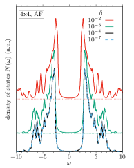
(b)

Figure 1: LABEL:sub@fig:e-trunc:sketch Schematic representation of the energy truncation. Overlaps $\epsilon_{n}=\langle\tilde{E}_{n}|\psi\rangle<\delta$ are neglected when constructing the sublattice projection (marked red). LABEL:sub@fig:e-trunc:dos Effect of the truncation threshold on the (lattice) density of states $N(\omega)$ for a $4\times 4$ cluster in the AF phase, see Sec.III.2 for details. The results for $\delta=10^{-2},10^{-3}$ are shifted for clarity.

Constructing Krylov spaces of higher order, an increasing number of highly excited states has to be captured by the MPS representations of the Krylov vectors. Unfortunately, states from the bulk of the many-body Hamiltonian’s spectrum typically satisfy a volume law of entanglement Bianchi et al. (2022) and are therefore the main reason for the exponentially increasing computational complexity. While this is a problem in general, here, we are interested in a faithful approximation of the poles of the Green’s matrix, i.e., their positions and weights. Hence, we can exploit a strategy introduced previously in the context of expanding the resolvent in terms of Chebyshev polynomials Holzner et al. (2011). The general idea is to construct local Krylov spaces at each lattice site and iteratively project the state’s site tensors into a sequence of local Krylov subspaces. However, in contrast to projecting the site tensors into a certain energy window as described in Holzner et al. (2011), we use the local Krylov space expansion to construct a projector to the subspace containing the most relevant eigenstates, up to a defined threshold $\delta$:

$$\ket{\psi}=\sum_{n}\underbrace{\braket{\tilde{E}_{n}}{\psi}}_{\varepsilon_{n}}\ket{\tilde{E}_{n}}\approx\sum_{\varepsilon_{n}>\delta}\varepsilon_{n}\ket{\tilde{E}_{n}}$$ (8)

where

$$\ket{\tilde{E}_{n}}=\sum_{l=0}^{K}c_{l}\ket{\nu_{l}}\;,\quad\lim_{K\rightarrow\operatorname{dim}\mathcal{H}}\hat{H}\ket{\tilde{E}_{n}}=E_{n}\ket{E_{n}}$$ (9)

and $\ket{\nu_{l}}\in\mathcal{H}_{K}$ Lanczos vectors in Krylov space $\mathcal{H}_{K}=\operatorname{span}\left\{\ket{\psi},\hat{H}\ket{\psi},\ldots,\hat{H}^{K}\ket{\psi}\right\}$. A schematic illustration of the energy truncation is shown in Fig. 1a. The red shaded bars correspond to those eigenstates that have a weight $\braket{\tilde{E}_{n}}{\psi}<\delta$ and are hence discarded. Refering to the expansion of the Green’s function in the Krylov subspace Eq. 7, we can identify the weights with the expansion of the matrix elements $\braket{k_{\alpha^{\prime}_{\nu^{\prime}},\nu^{\prime}}}{\hat{c}^{\dagger}_{\mu}}{\psi}$ in the energy eigenbasis. The energy truncation thus simply discards those eigenstates, whose contribution to the total Green’s function are $\mathcal{O}(\delta^{2})$.

In Fig. 1b we illustrate the effect of the energy truncation on the calculated lattice density of states using the CPT Green’s function for a $4\times 4$ cluster in the antiferromagnetically ordered state. Setting the truncation threshold too high results in a breakdown of the subspace projection. Here, this is the case for $\delta=10^{-2}$, where the erroneous subspace projection leads to a density of states, which neither captures correctly the gap nor the high-frequency part of the spectrum. However, already for moderate values of $\delta\lesssim 10^{-3}$ the spectrum is well reproduced, in particular the gap and the low-energy part of the spectrum, and only small deviations from the exact result are visible for higher excitation energies. A truncation threshold of $\delta\leq 10^{-4}$ finally leads to results which are for practical purposes essentially exact. In this case, only states with negligible weight for the density of states are truncated. The systematic improvements of the high-energy part of the spectrum can be related to the fact that the Green’s function is computed from locally exciting the ground state, such that the weight of higher-energy eigenstates decreases rapidly. For the following calculations, we avoid any ambiguity by using an energy truncation threshold of $\delta=10^{-5}$.

The computational costs of this energy truncation are not negligible. The complexity per local update scales as $\mathcal{O}(Km^{3}wd)+\mathcal{O}(Km^{2}w^{2}d^{2})$ where $K$ is the number of applications of the local representation of $\hat{H}$. Refering to standard notation, here we denote the MPS bond dimension by $m$, the MPO bond dimension by $w$ and the local Hilbert space dimension by $d$. Thus, we use the energy truncation only for the large clusters with $L\geq 16$ sites and apply it in the process of creating a new candidate state only once, namely after the global application of $\hat{H}$. However, the goal is not to achieve a speed up at constant $m$. Instead, we aim for a reduction of orthogonality losses that occur when orthogonalizing candidate states with respect to each other. Here, the effect of the energy truncation is to remove highly entangled contributions allowing for signficantly higher precision in the orthogonalization procedure, while keeping the bond dimension fixed. We found that building up a reasonably large Krylov space of dimension $D\sim 100$ for the larger clusters using computationally feasible bond dimensions $m=1024-2048$ was possible only when employing an energy truncation. Otherwise, orthogonality could not be maintained and the construction procedure would break down due to orthogonality losses.

III.1.2 Hochbruck-Lubich criterion

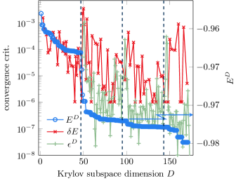
Figure 2: Comparison of convergence critera. The blue curve (right $y$-axis) shows the lowest eigenvalue $E^{D}$ of the effective Hamiltonian in the Krylov subspace as a function of the dimension $D$ for a $4\times 6$-site Hubbard cluster at $U=8t$ and a staggered magnetic field $h_{z}=0.09t$. The conventional convergence criterion $\delta E=E^{D+1}-E^{D}$ is given by the red line (left $y$-axis), exhibiting strong fluctuations over several orders of magnitude. In contrast, oscillations in the suggested Hochbruck-Lubich critertion $\epsilon^{D}$ shown by the green line are significantly smaller, overlaying a systematic decrease w.r.t. the number of iterations.

Controlling the convergence of the band Lanczos in the MPS representation is a suprisingly delicate problem. The unavoidable loss of numerical precision, caused by performing global operations using MPS arithmetics, as well as finite truncation errors, render standard convergence criteria such as the relative change in the ground-state energy in the constructed Krylov subspace not suitable. For instance, initially one observes a steep decrease of the relative error $\delta E=(E^{D+\alpha+1}-E^{D+\alpha})/E^{D+\alpha}$, where $E^{D+\alpha}$ is the ground state energy after adding the $\alpha$th candidate state to the Krylov subspace $\mathcal{K}^{D}_{\sigma}$. However, $\delta E$ exhibits rather drastic jumps over more than an order of magnitude, paired with iterations where $\delta E=0$ w.r.t. the energy resolution, which is bounded by the MPS truncation error. This phenomenon is shown at the example of a $4\times 6$-Hubbard cluster in Fig. 2 where the red curves represent $\delta E$.

There are two major sources for an erroneous convergence indication in $\delta E$. First, whenever $\hat{H}$ is applied to a complete sequence of candidate states (here, $N\cdot 2L=N\cdot 48$ marked by the dashed lines), the Krylov order $N$ increases. Given a fixed Krylov order, the band Lanczos generates a sequence of states that optimize the approximation of the ground state, which, however, is constraint by the Krylov order. Therefore, $\delta E$ decreases within a sequence of candidate states, which leads to a false indication of overall convergence. Second, candidate states $\ket{k_{\alpha,N}}$ have a different relevance for the ground state approximation. Most prominently, states that are created from initial excitations located at the boundary of the system converge more quickly.

Besides these technical problems, in practise the energy gain is not the most relevant quantity: In the end, the goal is to approximate the poles and weights of the cluster Green’s function up to a certain precision. For that purpose, here we pursue a different approach using a convergence criterion that directly measures the desired approximation quality. The idea is to relate an error measure $\delta R^{D}(\tau)$, which can be derived for the approximation of the action of the operator exponential $\mathrm{e}^{-\mathrm{i}\hat{H}\tau}\ket{\psi}$ to the Green’s function. The detailed derivation is given in App. B, here we only quote the resulting bound for the error in approximating the Green’s function in the Krylov subspace with dimension $D$:

$$\lvert\delta G^{(e,h)}_{\mu\nu}(\omega)\rvert\leq 2\pi^{2}\delta R^{D}(\tau)\;.$$ (10)

$\delta R^{D}(\tau)$ can be approximated by the generalized residual introduced by Hochbruck and Lubich Hochbruck and Lubich (1997, 1999); Botchev et al. (2013), which bounds the actual approximation error of the operator exponential $\epsilon^{D}\leq\delta R^{D}(\tau)$. An estimation for $\epsilon^{D}$ is given by the Hochbruck-Lubich bound Hochbruck and Lubich (1999)

$$\epsilon^{D}_{\tau}\leq\frac{40}{\tau}e^{-\frac{\tau}{4}}\left(\frac{e\tau}{4D}\right)^{D}\;,$$ (11)

relating the approximation error of the cluster Green’s function to the Krylov space dimension $D$ and the chosen time step $\tau$. In our computations, we choose $\epsilon\leq\delta R^{D}(\tau)$ as error threshold, which can be evaluated at negligible numerical costs from the matrix representation of the exponential of the effective Hamiltonian $\hat{H}^{D}$ Botchev et al. (2013); Paeckel et al. (2019) (see also App. B). We furthermore fix the time step by relating it to the spectral width $W$ of $\hat{H}$ via $\tau=\frac{2\pi}{\kappa W}$ where typically we choose the energy window fraction $\kappa\approx 1$.

We can now argue why we expect this error measure to be more reliable than only considering the relative change in the ground-state energy: $\delta R^{D}(\tau)$ is not a relative measure and while we also found it to exhibit fluctuations in our numerics, these are less severe than those in $\delta E$. The stability of $\delta R^{D}(\tau)$ against fluctuations comes from the fact that increasing the Krylov space dimension $D$, the residual in approximating the time evolution is monotonically decreasing, which follows directly from Eq. 11. Thus, fluctuations can only be generated from approximation errors caused by the MPS arithmetics and truncation errors. The main effect of these errors is to destroy the block-tridiagonal form of the effective Hamiltonian, which, however, can be monitored by the precision of the MPS arithmetics and the truncation errors. We choose the corresponding thresholds to be sufficiently small and thereby obtain a significantly more stable convergence criterion than using $\delta E$. It should be noted that strictly speaking, Eq. 11 is valid only after a complete sequence of Lanczos states for the set of initial states $\ket{\varphi^{(e)}_{j,\sigma}}$ has been constructed, i.e., the Krylov space dimension has to fulfill $D=N\cdot L$. We discuss this issue in App. B but from our numerical experience we found that the violation of monotonicity while constructing a new set of $L$ candidate states is not too severe.

III.1.3 Orthogonality loss

A major source for numerical instabilities in Krylov subspace methods is the loss of orthogonality of Krylov vectors. While in the commonly used exact state-representations the loss of orthogonality is in general caused by round-off errors due to finite-precision arithmetics Meurant and Strakoš (2006), the use of MPS introduces additional error sources. On the one hand, generating a new set of candidate states in the $N$th iteration of the band Lanczos recursion requires to act with the Hamiltonian on MPS representations of Lanczos vectors $\ket{k_{\alpha,N}}$: $\ket{k_{\alpha,N}}\longmapsto\hat{H}\ket{k_{\alpha,N}}$. Performing this operation by a naïve MPO -MPS application is numerically very costly so that we resort to a variational application scheme with a zipup-preconditioner Paeckel et al. (2019). While this allows us to achieve convergence of the MPO -application typically after two sweeps, we are still limited by the growth of the MPS bond-dimension, requiring a finite truncated weight. On the other hand, the orthogonalization of new candidate vectors $\hat{H}\ket{k_{\alpha,N}}$ against previous Lanczos states has to be done using a variational update scheme at finite truncated weight, too. This introduces a further loss of numerical precision if the variational optimization can get stuck in local minima. We preconditioned the optimization using an optimized initial guess state generation by mixing small contribution of higher and lower order Krylov states into the candidates. Nevertheless, the band Lanczos recursion inevitably is going to loose orthogonality, and the rate at which this loss occurs crucially depends on the maximally allowed truncated weight.

In order to keep the recursions stable as long as possible, we exploit the energy truncation, which removes poles, i.e., eigenstates, with small weights in the Green’s function from the Lanczos states. This truncation then allows us to use small truncated weights $\delta_{\mathrm{trunc}}\sim\mathcal{O}(10^{-10})$ at moderate bond dimensions. We typically allow for up to $\chi_{\mathrm{max}}=1024$ states and only for the very large clusters increased that value to $\chi_{\mathrm{max}}=2048$. Throughout the band Lanczos recursion, we then monitor the violation of the anti-commutation relations

$$\mathcal{I}_{j,\sigma;j^{\prime},\sigma^{\prime}} =\sum_{\alpha,\nu}\braket{0}{\hat{c}^{\dagger}_{j,\sigma}}{k_{\alpha,\nu}}\braket{k_{\alpha,\nu}}{\hat{c}^{\phantom{\dagger}}_{j^{\prime},\sigma^{\prime}}}{0}$$

$$\phantom{=}\quad+\braket{0}{\hat{c}^{\phantom{\dagger}}_{j^{\prime},\sigma^{\prime}}}{k_{\alpha,\nu}}\braket{k_{\alpha,\nu}}{\hat{c}^{\dagger}_{j,\sigma}}{0}\;.$$ (12)

We consider a deviation

$$\delta_{\mathrm{ol}}=\sqrt{\sum_{j,j^{\prime}}\sum_{\sigma,\sigma^{\prime}}\lVert\mathcal{I}_{j,\sigma;j^{\prime},\sigma^{\prime}}-\delta_{j,j^{\prime}}\delta_{\sigma,\sigma^{\prime}}\lVert^{2}}<10^{-3}\;,$$ (13)

which is of the order of the total truncation error $\sim L\cdot\sqrt{\delta_{\mathrm{trunc}}}$, as acceptable and terminate the Lanczos recursion if that threshold is exceeded. For all practical applications discussed in this paper, the energy truncation allowed us to perform $\sim\mathcal{O}(100)$ Lanczos iterations without facing numerical instabilities caused by the orthogonality loss. Importantly, this number was sufficient to converge also the largest clusters and obtain faithful approximations of the relevant poles and weights of the cluster Green’s function w.r.t. the convergence criterion introduced in Sec. III.1.2.

III.1.4 Energy rescaling

In order to conveniently use the error bound Eq. 11 we always rescale the Hamiltonian such that the spectral width is given by $W\equiv 1$. Furthermore, the rescaling allows us to introduce another tool to control the quality of the constructed Krylov subspace. In fact, a severe loss of orthogonality in the band Lanczos is typically signalled by an artificial drop of the lowest eigenvalue $\tilde{E}^{D}_{0}$ of the effective Hamiltonian in the Krylov space $\mathcal{K}^{D}$ below the ground-state energy. For these reasons we rescale and shift the Hamiltonian $\hat{H}$ throughout our computations, which of course needs to be compensated for in the evaluation of the cluster Green’s function. The first step of the rescaling is to obtain the spectral width

$$W=\lvert E_{0}-E_{\mathrm{max}}\rvert$$ (14)

of $\hat{H}$ by calculating the ground-state energy $E_{0}$ and the energy of the highest excited state $E_{\mathrm{max}}$. Afterwards, the Hamiltonian is rescaled and shifted,

$$\hat{H}\rightarrow\hat{\tilde{H}}=\frac{\hat{H}-E_{\mathrm{max}}}{\lvert E_{0}-E_{\mathrm{max}}\rvert}\;,$$ (15)

to force the spectrum to be located within the interval $[-1,0]$. Thus, the lowest eigenvalue of the effective Hamiltonian serves as additional proxy to the convergence of the Krylov-space by monitoring whether the condition $\tilde{E}^{D}_{0}>-1$ holds true. We also note that using the rescaled Hamiltonian, the Hochbruck-Lubich time step is related trivially to the energy window fraction $\tau=2\pi/\kappa$.

III.2 VCA

The VCA Potthoff et al. (2003) is an established quantum-cluster technique, which is well-suited to probe correlated systems for symmetry-breaking fields Dahnken et al. (2004a); Sénéchal et al. (2005a). It is based on the self-energy-functional (SEF) theory Potthoff (2003a, b, 2012) and consists of determining the stationary points of the SEF $\Omega_{\mathbf{t}}[\mathbf{\Sigma}]$, which is related to the Baym-Kadanoff-Luttinger-Ward functional Baym and Kadanoff (1961); Luttinger and Ward (1960), with respect to trial self-energies of a reference system $\mathbf{\Sigma}(\mathbf{t}^{\prime})$:

$$\Omega_{\mathbf{t}}\left[\mathbf{\Sigma}\left(\mathbf{t}^{\prime}\right)\right]= \Omega^{\prime}+\Tr\ln\left(-\left(\mathbf{G}_{0}^{-1}-\mathbf{\Sigma}\left(\mathbf{t}^{\prime}\right)\right)^{-1}\right)$$

$$-\Tr\ln\left(-\mathbf{G}^{\prime}\right)\;.$$ (16)

Here, $\Tr\mathbf{A}=T\sum_{\omega,\alpha}A_{\alpha,\alpha}(i\omega)$, $\Omega^{\prime}$ denotes the grand potential, and $\mathbf{G}^{\prime}$ the Green’s function of the reference system. Since the theory requires the reference system to have the same interaction terms as the original system, the cluster self-energies can be varied via their one-body terms $\mathbf{t}^{\prime}$. At a stationary point, the SEF represents an approximation of the grand potential of the original system in the variational space of available self-energies of the reference system.

To investigate symmetry-broken phases, a (fictitious) symmetry-breaking Weiss field term can be added to the cluster Hamiltonian. The Weiss field strength is then one of the one-body terms, which are determined via the variational principle that leads to stationarity of the SEF with respect to the cluster self-energy.

Here, we focus on zero temperature, $T=0$, and perform the summation over frequency $\omega_{m}$ in Eq. 16 analytically. In this case one obtains Aichhorn et al. (2006a)

$$\Tr\ln(\mathbf{G}_{0}^{-1}-\mathbf{\Sigma})^{-1} =\sum_{m}\omega_{m}\Theta(-\omega_{m})-R$$ (17)

$$\Tr\ln\mathbf{G^{\prime}}^{-1} =\sum_{m}\omega_{m}^{\prime}\Theta(-\omega^{\prime}_{m})-R\;,$$ (18)

with the Heaviside function $\Theta(\omega)$, a contribution $R$ from the poles of the self-energy, the poles $\omega^{\prime}_{m}$ of the cluster Green’s function $\mathbf{G}^{\prime}$, and the poles $\omega_{m}$ of the VCA Green’s function $(\mathbf{G}_{0}^{-1}-\mathbf{\Sigma})^{-1}$. It is therefore useful to work with a Lehmann representation of the Green’s function since it explicitly includes the information about its poles $\omega_{m}$; for more details see appendix A.

In order to limit the variational space of cluster self-energies, a limited set of one-body parameters of the cluster Hamiltonian are varied in practice: The hopping strengths $t^{\mathrm{cluster}}_{ij}$ can be determined from the variational principle to account for cluster boundary effects Potthoff et al. (2003), whereas the cluster chemical potential $\mu^{\prime}$ should be optimized to obtain a thermodynamically stable electron filling $n$ Aichhorn et al. (2006b). Additional one-body terms can be added to the cluster Hamiltonian to account for symmetry-broken phases such as magnetic order Dahnken et al. (2004b), superconductivity Sénéchal et al. (2005b) or charge order Aichhorn et al. (2004).
In the half-filled two-dimensional Hubbard model with isotropic nearest-neighbor hopping, the chemical potential is at $\mu=U/2$ and $\mu^{\prime}$ does not need to be determined in the variational search. Furthermore it was shown that optimizing the cluster hopping terms did not lead to significant improvement of the approximation of the grand potential Potthoff et al. (2003). To capture the essential physics of antiferromagnetic ordering, it is therefore sufficient to apply a staggered magnetic field of strength $h_{z}$ on the cluster, see Eq. (3), and use it as the sole one-body parameter throughout the variational search.

III.3 Choice of clusters

The choice of a cluster is a centerpiece of most quantum cluster techniques be it for accessing specific cluster momenta or for performing a finite-size scaling. Besides the size of the cluster, its geometry is of crucial importance in two-dimensional systems and the seminal papers of Betts et al. Betts et al. (1996a, 1999) introduced a set of evaluation criteria for the suitability of clusters with periodic boundary conditions, which were based on the completeness of near-neighbor shells.

Within CPT and VCA one uses open boundary conditions on the clusters and a systematic study of Betts clusters is missing. Nevertheless, we resort here to the labelling and characterization scheme introduced by Betts et al. Betts et al. (1996b), in particular to parameters such as the geometrical imperfection $J$ and the bipartite imperfection $I_{B}$ to identify clusters of high geometrical and topological quality. Apart from more traditional rectangular clusters, we also test our solver on skewed Betts clusters. We limit ourselves to clusters that can tile bipartite lattices and focus on those which have zero bipartite imperfection. By combining calculations of several cluster geometries, we can access different points of the lattice Brillouin zone via reciprocal vectors of the superlattice. In Fig. 3 we illustrate this for lattice tilings using different 24-site clusters that fulfil the condition $I_{B}=0$.

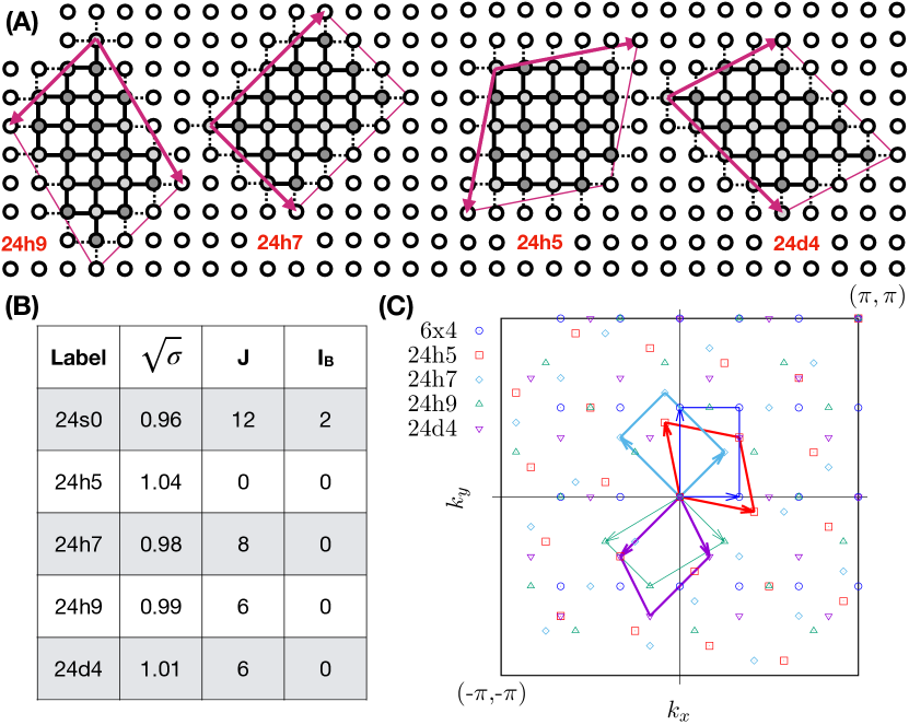
Figure 3: (A) Illustration of the geometries of different clusters with $N=24$ sites labeled according to Betts et al. Betts et al. (1996b). Red arrows indicate the superlattice vectors that tile the lattice with the respective cluster, dashed lines indicate inter-cluster hopping terms and the Néel-type sublattice structure is indicated by different tones of grey. The clusters differ in their squareness ${\sigma}$, geometrical imperfection $J$ and bipartite imperfection $I_{B}$, see (B). (C) Points in the Brillouin zone that are multiples of reciprocal superlattice vectors, which are indicated by arrows. The corresponding reduced (superlattice) Brillouin zones are marked by parallelograms.

IV Results and discussion

In the following, we study the antiferromagnetic (AF) ordering within the half-filled single-band Hubbard model to benchmark our solver. We focus here at the challenging point in parameter space $U/t=8$, i.e., an on-site interaction equal to the band-width of the non-interacting dispersion, where the system is already in the Mott insulating regime.

Translated to the self-energy functional, this leads to one stationary point, a maximum, at $h_{z}=0$ corresponding to a non-magnetic solution and to two minima at $h_{z}=\pm h_{z}^{c}\neq 0$ corresponding to a phase with antiferromagnetic order, see Fig. 4. Since $\Omega$ is symmetric in $h_{z}$, we plot it in the following only for positive values of $h_{z}$.

Compared to numerically exact solvers, the MPS -based solver introduces additional approximations, in particular since the MPS bond dimension is bound to a maximal value $\chi^{\mathrm{max}}$ and since perfect orthogonality between the Krylov vectors is lost faster at large iteration numbers within the band-Lanczos procedure. Comparing the self-energy functional computed with our MPS-based solver to the benchmark using an exact diagonalization (ED) based solver, we see excellent agreement in Fig. 4 if the maximal MPS bond dimension is chosen large enough. For the small cluster used here, $\chi$ can be increased until the MPS representation is essentially exact. However, for too small bond dimension, deviations from the exact curve are visible. In that case, the self-energy functional is systematically evaluated to be too large. Except for extreme cases, e.g. $\chi=128$ in Fig. 4, $\Omega$ shows even for moderate bond dimension correct functional behavior as a function of the Weiss field, which allows for an interpolation around the stationary points. As we show in Sec. IV.0.1, fitting the self-energy functional to determine its stationary points allows to calculate observables for different bond dimension in order to perform an extrapolation to $\chi^{\mathrm{max}}\rightarrow\infty$.

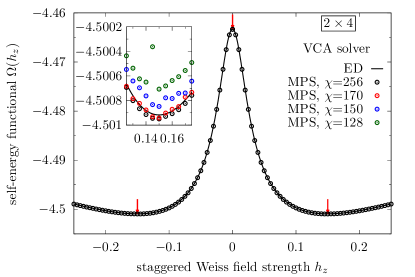
Figure 4: The self-energy functional $\Omega$ as a function of staggered Weiss field strength for a $2\times 4$ cluster. Stationary points of $\Omega$ are indicated by arrows. Dots denote results obtained with the matrix-product state (MPS)-based solver, in the inset shown for different maximal MPS bond dimension $\chi^{\mathrm{max}}$ around the minimum of $\Omega$; the results obtained with an exact diagonalization (ED) solver are shown as a line.

To illustrate the effects of cluster geometry on $\Omega$, we plot in Fig. 5 the self-energy functional of the 24-site clusters introduced in Fig. 3. Even though the rough functional forms of $\Omega$ do not differ qualitatively, their stationary points vary notably. We also note that clusters with similar geometric properties, as for instance quantified in terms of their geometrical and bipartite imperfection, see Fig. 3(B), generate quite similar self-energy functionals, whereas different imperfection of two clusters leads to significantly different $\Omega$.

Another consequence of using a MPS representation of the quantum states is that even for a given cluster geometry, the obligatory mapping of the 2D cluster onto a 1D chain introduces a degree of freedom which has a direct impact on the precision with which the SEF is calculated. In the inset of Fig. 5 we illustrate this effect by calculating the cluster Green’s function of the rectangular 24s0 cluster for two different 1D mappings. The corresponding self-energy functionals agree in the $\chi\rightarrow\infty$ limit, but differ for finite $\chi$. Whereas the mapping minimizing long-range hopping (’$4\times 6$’) leads to well converged results at $\chi^{\mathrm{max}}=1024$, the longer-ranged mapping (’$6\times 4$’) leads to a larger build-up of entanglement and would require a $\chi^{\mathrm{max}}>2048$.

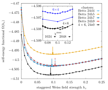
Figure 5: Impact of the cluster geometry on the self-energy functional. $\Omega$ is calculated with $\chi^{\mathrm{max}}=1024$ for different 24-site clusters shown in Fig. 3. Minima of $\Omega$ are indicated by arrows, lines are only a guide to the eye. The inset shows $\Omega$ for two different 1D mappings of the 24s0 cluster, ’$4\times 6$’ and ’$6\times 4$’, calculated with $\chi^{\mathrm{max}}=1024,2048$.

In presence of nearly degenerate quantum states, different symmetry-breaking orders on the cluster can be easily picked up within MPS based approaches when not providing a sufficiently large bond dimension. This is for instance the case for the ’$4\times 6$’ mapped 24s0 cluster at $h_{z}\approx 0.11$, see inset of Fig. 5. Hence, scaling the position of the stationary points of $\Omega$ in the maximal MPS bond dimension instead of individual points of the self-energy functional proved to be more robust.

IV.0.1 SEF scaling with bond dimension

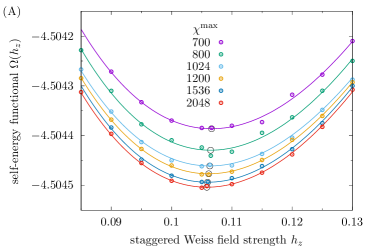
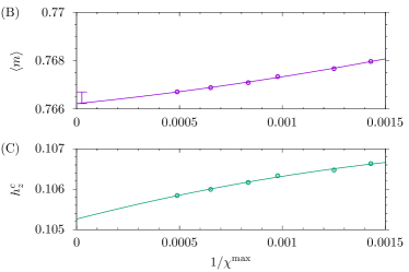
Figure 6: Scaling of the self-energy functional $\Omega$ in the maximal MPS bond dimension $\chi^{\mathrm{max}}$ for the Betts cluster 22h5. Around the stationary point $\Omega(h_{z}^{c})$ the functional can be fitted as a function of the Weiss field, shown as a line (A); the corresponding minima are indicated by black circles. For different $\chi^{\mathrm{max}}$, the SEF shows similar functional dependence on $h_{z}$. The staggered magnetization $\langle m\rangle$ on the lattice (B) and the Weiss field strength $h_{z}^{c}$ (C) are then scaled as a function of inverse bond dimension $1/\chi^{\mathrm{max}}$.

In Fig. 6, the value of the Weiss field $h_{z}^{c}$ as well as the staggered magnetization on the lattice, $\langle m\rangle$, are scaled in the inverse bond dimension. The staggered magnetization scales linear in $1/\chi^{\mathrm{max}}$ and gives a lower estimate of the expectation value for the $\chi^{\mathrm{max}}\rightarrow\infty$ limit. Since at some critical $\chi^{c}$ the MPS representation is exact, we expect a constant value of $\langle m\rangle$ for $\chi^{\mathrm{max}}>\chi^{c}$. The value of $\langle m\rangle$ at the largest calculated $\chi^{\mathrm{max}}$ therefore sets an upper bound for the staggered magnetization.

However, the dependence of $h_{z}^{c}$ and $\langle m\rangle$ on $1/\chi$ is mild ($\mathcal{O}(10^{-3})$) and of the same order as the estimated error such that it can be neglected in practice for most applications as long as a sufficiently large bond dimension $\chi$ is used. In the case of the shown 22-site Betts cluster, this would be the case for $\chi^{\mathrm{max}}\gtrsim 1000$. Given the large computational cost of evaluating the cluster Green’s function via the MPS-based band Lanczos solver, systematically scaling expectation values in the MPS bond dimension should remain the exception. Instead, it offers the possibility to calculate spectral functions or observables for large clusters (e.g. using cluster perturbation theory), for which symmetry breaking terms can be included via VCA. The rather mild dependence of the functional form of the SEF and the related expectation values on the chosen MPS bond dimension is important in this context.

IV.0.2 Spectral functions

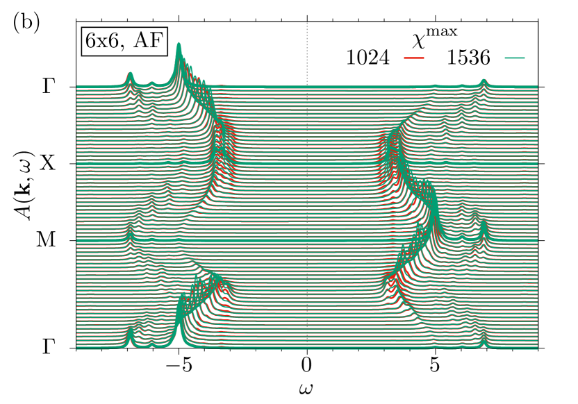
Figure 7: (a) Density of states $N(\omega)$ of the $4\times 4$ (top) and 22h5 (bottom) clusters for different maximal MPS bond dimension $\chi^{\mathrm{max}}$. (b) shows the $\mathbf{k}-$resolved spectral function $A(\mathbf{k},\omega)$ of a $6\times 6$ cluster for two different maximal bond dimensions. All calculations were done in the antiferromagnetically ordered state, i.e. at the stationary point of the SEF for the respective clusters.

Next, we discuss the mild influence of the maximal MPS bond dimension $\chi^{\mathrm{max}}$ on the spectral function, see Fig. 7.

For comparatively small clusters, the spectral function $A(\mathbf{k},\omega)$ and the density of states (DOS) $N(\omega)$ can be converged in $\chi^{\mathrm{max}}$. We illustrate this in the case of the $4\times 4$ cluster for $N(\omega)$ in Fig. 7(a). The results obtained from restricting the bond dimension to $\chi^{\mathrm{max}}=512$ show already good agreement for excitation energies close to the gap, but the density of states still shows differences at larger excitation energies around $\omega\sim\pm 6$. For $\chi^{\mathrm{max}}\gtrsim 1024$, the density of states and spectral function of the $4\times 4$ cluster are converged and do not change any more when increasing the bond dimension.

For larger clusters like the $22h5$ cluster discussed previously in Fig. 6, scaling $h_{z}^{c}$ and $\langle m\rangle$ still leads to minor changes when increasing the bond dimension up to $\chi^{\mathrm{max}}=2048$. However, tracking the changes of the density of states as a function of $\chi^{\mathrm{max}}$ reveals that only small changes close to the outmost band edges far from the gap are visible. The DOS for excitation energies $|\omega|\lesssim 5$ is already converged for $\chi^{\mathrm{max}}=1536$ and even for $\chi^{\mathrm{max}}=1024$ the deviations from the converged solution are for most purposes negligible.

In Fig. 7(b) we finally show the $\mathbf{k}-$resolved spectral function $A(\mathbf{k},\omega)$ along the high symmetry path $(0,0)-(\pi,0)-(\pi,\pi)-(0,0)$ for one of the largest clusters we systematically studied, the $6\times 6$ cluster. The spectral function was calculated from the CPT Green’s function, Eq.(2), using the periodization scheme proposed in Ref. Sénéchal et al., 2000. In contrast to small and intermediate clusters, the SEF of the $6\times 6$ cluster still shows notable differences as a function of the MPS bond dimension up to $\chi^{\mathrm{max}}=2048$. They translate to the spectral function in form of small differences in the low-energy excitations, most visible around the X point, $\mathbf{k}=(\pi,0)$. Nevertheless, the most salient features of the spectral function are already converged in the bond dimension for a remarkably small $\chi^{\mathrm{max}}=1536$. This can be seen as an advantageous feature of the MPS solver, which enforces due to the energy truncation scheme first the convergence of poles of the Green’s function that contribute most spectral weight. The present MPS solver therefore even allows to interpret spectral functions of large clusters for which a full convergence in terms of the MPS bond dimension cannot be achieved.

IV.0.3 Finite size scaling

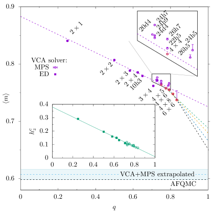
Figure 8: Finite-size scaling of VCA data for different rectangular and Betts clusters. The staggered magnetization $\langle m\rangle$ and the magnetic Weiss field on the cluster $h_{z}$ (inset) are scaled as a function of the parameter $q$ described in text. The reference data from auxiliary-field quantum Monte Carlo (AFQMC) is taken from Ref. Seki and Sorella (2019). The staggered magnetization extrapolated from the band-Lanczos results for rectangular clusters (highlighted in red) using a non-linear ansatz is shown as dashed blue line and the shaded area indicates the $1\sigma$ confidence interval, containing the AFQMC result.

In order to perform a finite-size scaling of the staggered magnetization, calculations need to be performed using different cluster sizes. However, even for fixed cluster size, the cluster geometry has an impact on the self-energy functional since the corresponding cluster Green’s functions include long-range correlations to a different extent. To include this information for the finite-size scaling, we use the quality factor introduced by D. Sénéchal in Ref. Sénéchal, 2008. It amounts to comparing the intra-cluster hopping terms $N_{t}^{cl}$ to the number of hopping terms per site in the infinite lattice and therefore takes into account both the cluster size and geometry. In the square lattice, this amounts to $q=N^{cl}_{t}/2L$. The scaling factor $q$ thereby contrasts with other commonly used scaling parameters like $1-1/L$, which include only information of the cluster size.

When using this quality factor, the extrapolation of the Weiss field strength $h^{c}_{z}$ to the thermodynamic limit leads to a vanishing field strength whereas the expectation value of the staggered magnetization on the lattice $\langle m\rangle$ extrapolates to a finite value, see Fig. 8. In the infinite-cluster-size limit, $q=1$ and we will not need the symmetry-breaking field since the symmetry will be broken spontaneously. There, the value of the staggered magnetization $\left.\langle m\rangle\right|_{q=1}$ simply corresponds to the order parameter on the lattice. At half-filling, $\langle m\rangle$ can be calculated numerically exactly using auxiliary-field quantum Monte Carlo simulations (AFQMC) Hirsch (1983); Sugiyama and Koonin (1986); Sorella et al. (1989); Imada and Hatsugai (1989); Rom et al. (1997); Becca and Sorella (2017).

Comparing to the AFQMC result (dashed black line) of Seki and Sorella Seki and Sorella (2019) we see that the linear scaling in $q$ (dashed, violet graph) would lead to an overestimation by $\sim 20\%$ of the staggered magnetization, i.e., the linear dependence $\langle m\rangle$ on $q$ seems to hold only for small and intermediate cluster sizes. Indeed, for the largest clusters calculated with our MPS band-Lanczos solver, we already observe a significant deviation from linear scaling (c.f. the red highlighted symbols in Fig. 8). We believe that besides others, the non-linear $q$-dependence is generated from the fact that in the presented calculations we did not vary the hopping amplitudes at the cluster boundaries. In that case, an extrapolation would still be possible even though the exact functional dependency is unknown.

We attempt to account for the non-linear behavior by: (1) Linearly extrapolating $\braket{m}(q\rightarrow 1,q_{0})$ for the largest rectangular clusters (c.f. the red highlighted symbols in Fig. 8) on a domain $[q_{0},1]$ where we varied $q_{0}\in[0.775,0.8125]$. The obtained linear extrapolations are indicated by the colored dashed lines in Fig. 8. (2) We then make the simplest non-linear ansatz for the functional dependency on $q_{0}$

$$\braket{m}(q\rightarrow 1,q_{0})=\alpha(q_{0}-1)^{2}+m_{\infty}\;.$$ (19)

This ansatz has a stationary point at $q_{0}=1$, resembling the expected asymptotic behavior of the magnetization when scaling the number of cluster sites to the thermodynamic limit. The extrapolated value of the magnetization is $m_{\infty}=0.607\pm 0.009$, which is shown in Fig. 8 as blue dashed line and the shaded area indicates the $1\sigma$ confidence interval of the extrapolation. Note that this value agrees with the AFQMC-result $m^{\mathrm{QMC}}_{\infty}=0.5982$ within the confidence interval and the deviation is only about $1.5\%$. We therefore find that with the cluster sizes accessible via the VCA +MPS ansatz, it is possible to estimate values for local observables in the thermodynamic limit to a very high precision, even without exploring all possible variational parameters within VCA.

V Conclusions and Outlook

We introduce a band-Lanczos solver based on MPS for quantum cluster methods such as the VCA. While a naïve implementation of MPS as cluster solver does not lead to a substantial improvement over using ED techniques, we showed that significantly larger cluster sizes can be treated with high accuracy by combining the MPS +band-Lanczos solver with a suitable energy truncation, controlling the loss of orthogonality of the Lanczos states and introducing a robust convergence criterion.

We demonstrate the potential of the approach by computing the staggered magnetization $\langle m\rangle$ of a single band Hubbard model on a 2D square lattice. Treating different cluster sizes and shapes (regular rectangular as well as Betts clusters), we extrapolate our MPS data in the bond dimension $\chi$, which we show to yield a systematic improvement of the approximation quality of the Green’s function and its derived quantities. In this way we can exploit the increased number of accessible cluster sizes and geometries to extrapolate observables such as the staggered magnetization into the thermodynamic limit. We show that at half filling and for intermediate interaction strengths $U/t=8$ (i.e., in the Mott insulating regime, where the interaction strength is of the order of the bandwidth of the noninteracting system) an anomalous finite-size scaling with a crossover length scale is observed. Only for rectangular cluster sizes that are large enough, i.e., $4\times 4$ and larger, a deviation from an otherwise linear scaling is obtained, which can be extrapolated towards the correct result in the thermodynamic limit. The resulting value of $\langle m\rangle$ in the thermodynamic limit agrees with numerically exact QMC data within an error margin of $1.5\%$. In contrast, with the smaller cluster sizes amenable to ED, the extrapolation in cluster size leads to a value, which overestimates the QMC result by $\sim 20\%$.

Given the significant increase of the number of cluster sites, we envisage that our approach has the potential to substantially improve the investigations in multi-band Hubbard-like models. Here, Hund’s coupling leads to an interplay between orbital, spin, and electronic degrees of freedom Georges et al. (2013); de’ Medici (2017), which affects material properties like superconductivity in nickelates and iron based superconductors, orbital selectivity in iron chalcogenides or optoelectronic and photovoltaic properties Lanatà et al. (2013); Villar Arribi and de’ Medici (2021); De Franco et al. (2018); Pham and Li (2017); Hepting et al. (2020); Li et al. (2019); Rahil et al. (2022); Tsai et al. (2016); Rahil et al. (2022). Although the interactions are local in nature, the higher complexity of these 2D systems poses an even stronger challenge to their theoretical description. While it is essentially impossible for ED -based solvers to treat cluster sizes large enough to perform meaningful studies on such multi-orbital systems, the MPS +band-Lanczos approach makes it possible to treat also systems with larger local Hilbert spaces in a controlled way, so that it appears natural to extend our approach to such multi-band situations.

Supplemental Materials: Matrix-product-state-based band-Lanczos solver for quantum cluster approaches

Appendix A $Q$-matrix formulation of the cluster Green’s function

To rewrite the cluster Green’s function, we use the $\mathbf{Q}$-matrix formulation of the Lehmann representation introduced in Ref. Zacher et al. (2002):

$$G^{\prime}_{\alpha,\beta}(\omega)=\sum_{m}\frac{Q^{{\phantom{\dagger}}}_{\alpha,m\vphantom{\beta}}Q^{\dagger}_{m,\beta}}{\omega-\omega^{\prime}_{m}}\;,$$ (A.1)

with $\alpha,\beta$ being compound site and spin indices, and excited states $m$. The $\mathbf{Q}$-matrix is defined as the concatenation of the electron and hole matrices

$$Q^{\vphantom{(e)}}_{\alpha,m}= \left(Q_{\alpha,r}^{(e)},Q_{\alpha,s}^{(h)}\right)\,,$$ (A.2)

$$Q_{\alpha,r}^{(e)}= \braket{0}{\hat{c}^{\vphantom{(e)}}_{\alpha}}{r}\,,$$ (A.3)

$$Q_{\alpha,s}^{(h)}= \braket{s}{\hat{c}^{\vphantom{(e)}}_{\alpha}}{0}\;,$$ (A.4)

where $\ket{0}$ is the ground state with energy $E_{0}$. The corresponding excitation energies needed in Eq. 18 read $\omega^{\prime}_{m}=\left(\omega^{(e)}_{r},\omega^{(h)}_{s}\right)=\left(E^{{\phantom{\prime}}}_{r}-E^{{\phantom{\prime}}}_{0},E^{{\phantom{\prime}}}_{0}-E^{{\phantom{\prime}}}_{s}\right)$. To obtain the poles $\omega$ for Eq. 17 we rewrite the VCA Green’s function as

$$\mathbf{G} =\frac{1}{\mathbf{G}_{0}^{-1}-\Sigma}=\frac{1}{(\mathbf{G}^{\prime})^{-1}-\mathbf{V}}$$ (A.5)

$$=\mathbf{Q}\frac{1}{\mathbf{g}^{-1}-\mathbf{Q}^{\dagger}\mathbf{V}\mathbf{Q}}\mathbf{Q}^{\dagger}\;,$$ (A.6)

where $\mathbf{g}^{-1}=\omega-\mathbf{\Lambda}$ with $\Lambda^{{\phantom{\prime}}}_{m,l}=\delta^{{\phantom{\prime}}}_{m,l}\omega^{\prime}_{m\vphantom{l}}$ so that the poles $\omega_{m}$ are nothing but the eigenvalues of $\mathbf{\Lambda}+\mathbf{Q}^{\dagger}\mathbf{V}\mathbf{Q}$. The $\mathbf{Q}$-matrix and the one-particle excitations $\omega^{\prime}$ are calculated via the band Lanczos algorithm.

Appendix B Hochbruck-Lubich convergence criterion

We consider the Greens function in its time integral representation

$$G_{AB}(\omega+\mathrm{i}\eta)=\mathrm{i}\int_{0}^{\infty}dt\braket{\varphi_{A}}{\mathrm{e}^{-\mathrm{i}(\hat{H}-\omega-\mathrm{i}\eta)t}}{\varphi_{B}}$$ (B.1)

for some Hamiltonian $\hat{H}$ and local perturbations of an initial state $\ket{\psi}$ generated from operators $\hat{A},\hat{B}$:

$$\ket{\varphi_{A}}=\hat{A}\ket{\psi}\quad\text{and}\quad\ket{\varphi_{B}}=\hat{B}\ket{\psi}\;,$$ (B.2)

where $\eta>0$ is a finite broadening. The error estimation by Hochbruck and Lubich is based on approximating the action of an operator exponential $\mathrm{e}^{-t\hat{A}}$ in a Krylov subspace $\mathcal{K}^{D}$ where $D\in\mathbb{N}$ denotes the dimension of the Krylov subspace

$$\lVert\mathrm{e}^{-t\hat{A}}\ket{\varphi}-\mathrm{e}^{-t\hat{A}^{D}}\ket{\varphi}\rVert\approx t\left\lvert\beta^{D}\braket{f^{D}}{\mathrm{e}^{-t\hat{A}^{D}}}{\varphi}\right\rvert=t\delta R^{D}(t)\;,$$ (B.3)

where $\beta^{D}$ is the usual Lanczos residual after $D$ iterations, $\hat{A}^{D}$ denotes the projection of $\hat{A}$ to $\mathcal{K}^{D}$ and $\delta R^{D}(t)$ can be estimated by the generalized residual Hochbruck and Lubich (1997, 1999); Botchev et al. (2013). Here, $\ket{f^{D}}$ is the component of the initial state $\ket{\varphi}$ projected into the orthogonal complement $\mathcal{K}^{D}_{\perp}=\mathcal{H}\setminus\mathcal{K}^{D}$ of the Krylov subspace

$$\ket{\varphi}=\hat{P}^{D}\ket{\varphi}+\hat{P}^{D}_{\perp}\ket{\varphi}\equiv\hat{P}^{D}\ket{\varphi}+\ket{f^{D}}\;,$$ (B.4)

with $\hat{P}^{D}_{(\perp)}$ being the projector into $\mathcal{K}^{D}$ ($\mathcal{H}\setminus\mathcal{K}^{D}$). The estimation is based on a finite time argument in the exponent, hence we use the following decomposition of the integration domain

$$\int_{0}^{\infty}dtF(t) =\left[\int_{0}^{\tau}dt+\int_{\tau}^{2\tau}dt+\cdots\right]F(t)$$

$$=\sum_{p=0}^{\infty}\int_{0}^{\tau}dtF(t+p\tau)\;.$$ (B.5)

Decomposing the expectation value $F(t)=\braket{\varphi}{\mathrm{e}^{-\mathrm{i}\hat{H}\tau}}{\varphi}$ into its components the Krylov subspace and the orthogonal complement using Eq. B.4

$$F(t) =\braket{\varphi}{\mathrm{e}^{-\mathrm{i}\hat{H}^{D}\tau}}{\varphi}+\braket{f^{D}}{\mathrm{e}^{-\mathrm{i}\hat{H}^{D}\tau}}{\varphi}\;,$$ (B.6)

and abbreviating $\hat{U}^{D}(t,\omega)=\mathrm{e}^{-\mathrm{i}(\hat{H}^{D}-\omega)t}$, we can rewrite the time integration as

$$G_{AB}(\omega+\mathrm{i}\eta) =\mathrm{i}\int_{0}^{\infty}dt\braket{\varphi_{A}}{\hat{U}^{D}(t,\omega)\mathrm{e}^{-\eta t}}{\varphi_{B}}+\delta G^{D}_{AB}\;,$$ (B.7)

with the residual

$$\delta G^{D}_{AB} =\mathrm{i}\sum_{p=0}^{\infty}\int_{0}^{\tau}dt\braket{f^{D}_{A}}{\hat{U}^{D}(t+p\tau,\omega)}{\varphi_{B}}\mathrm{e}^{-\eta(t+p\tau)}\;.$$ (B.8)

We can now apply Eq. B.3 to estimate the residual

$$\lvert\delta G^{D}_{AB}\rvert \approx\int_{0}^{\tau}dt\sum_{p=0}^{\infty}(t+p\tau)\delta R^{D}(t+p\tau)\mathrm{e}^{-\eta(t+p\tau)}$$

$$\leq\delta R^{D}(\tau)\int_{0}^{\tau}dt\sum_{p=0}^{\infty}(t+p\tau)\mathrm{e}^{-\eta(t+p\tau)}$$

$$=\delta R^{D}(\tau)\frac{1-\mathrm{e}^{-\eta\tau}(1+\eta\tau)}{\eta^{2}}\;,$$ (B.9)

where we used the monotonicity of the generalized residual $\delta R^{D}(t)\leq\delta R^{D}(t+p\tau)\leq 1$ for $t\leq\tau$. In our numerical calculations we usually set $\tau=2\pi$ such that we can determine the correction term $J(\eta)\equiv\frac{1-\mathrm{e}^{-2\pi\eta}(1+2\pi\eta)}{\eta^{2}}$ in the limit $\eta\rightarrow 0$

$$\lim_{\eta\rightarrow 0}J(\eta) =\lim_{\eta\rightarrow 0}\frac{1-(1-4\pi^{2}\eta^{2})-2\pi^{2}\eta^{2}}{\eta^{2}}+\mathcal{O}(\eta)$$

$$=2\pi^{2}\;,$$ (B.10)

and thus we arrive at the error bound

$$\lvert\delta G^{D}_{AB}\rvert\leq 2\pi^{2}\delta R^{D}(\tau)\approx 20\cdot\delta R^{D}(\tau)\;.$$ (B.11)

The generalized residual $\delta R^{D}(\tau)$ can be computed at no additional cost using the approximation of the exponential in the Krylov subspace

$$\delta R^{D}(\tau)=\beta^{D}\braket{f^{D-1}}{\mathrm{e}^{-\mathrm{i}\hat{H}^{D}\tau}}{f^{D}}\;.$$ (B.12)

While these considerations provide a reliable bound for the usual Lanczos procedure, they are exact in case of the band Lanczos only, if the Krylov dimension $D$ and the Krylov order $N$, i.e., the number of applications of $\hat{H}$ to the set of $L$ initial states, are related via $D=N\cdot L$. The reason behind this limitation is that in Eq. B.6 we assumed that the residual Krylov vector $\ket{f^{D}}$ has a Krylov order $N+1$ while $\hat{H}^{D}$ is approximated with Krylov order $N$, only. In princple this means that Eq. B.11 can only be applied after a whole sequence of $L$ candidate states has been constructed. However, in practise we observed that also within such a sequence, Eq. B.11 yields satisfying error estimations with fluctuations in the error estimation being of an order of magnitude, at the most.

References

- Bednorz and Müller (1986) J. G. Bednorz and K. A. Müller, Zeitschrift für Physik B Condensed Matter 64, 189 (1986).
- Dagotto (1994) E. Dagotto, Rev. Mod. Phys. 66, 763 (1994).
- LeBlanc et al. (2015) J. P. F. LeBlanc, A. E. Antipov, F. Becca, I. W. Bulik, G. K.-L. Chan, C.-M. Chung, Y. Deng, M. Ferrero, T. M. Henderson, C. A. Jiménez-Hoyos, E. Kozik, X.-W. Liu, A. J. Millis, N. V. Prokof’ev, M. Qin, G. E. Scuseria, H. Shi, B. V. Svistunov, L. F. Tocchio, I. S. Tupitsyn, S. R. White, S. Zhang, B.-X. Zheng, Z. Zhu, and E. Gull (Simons Collaboration on the Many-Electron Problem), Phys. Rev. X 5, 041041 (2015).
- Zheng et al. (2017) B.-X. Zheng, C.-M. Chung, P. Corboz, G. Ehlers, M.-P. Qin, R. M. Noack, H. Shi, S. R. White, S. Zhang, and G. K.-L. Chan, Science 358, 1155 (2017), https://www.science.org/doi/pdf/10.1126/science.aam7127 .
- Cao et al. (2018) Y. Cao, V. Fatemi, S. Fang, K. Watanabe, T. Taniguchi, E. Kaxiras, and P. Jarillo-Herrero, Nature 556, 43 (2018).
- Lu et al. (2019) X. Lu, P. Stepanov, W. Yang, M. Xie, M. A. Aamir, I. Das, C. Urgell, K. Watanabe, T. Taniguchi, G. Zhang, A. Bachtold, A. H. MacDonald, and D. K. Efetov, Nature 574, 653 (2019).
- Cao et al. (2020) Y. Cao, D. Rodan-Legrain, O. Rubies-Bigorda, J. M. Park, K. Watanabe, T. Taniguchi, and P. Jarillo-Herrero, Nature 583, 215 (2020).
- Manzeli et al. (2017) S. Manzeli, D. Ovchinnikov, D. Pasquier, O. V. Yazyev, and A. Kis, Nature Reviews Materials 2, 17033 (2017).
- Ortiz et al. (2019) B. R. Ortiz, L. C. Gomes, J. R. Morey, M. Winiarski, M. Bordelon, J. S. Mangum, I. W. H. Oswald, J. A. Rodriguez-Rivera, J. R. Neilson, S. D. Wilson, E. Ertekin, T. M. McQueen, and E. S. Toberer, Phys. Rev. Mater. 3, 094407 (2019).
- Ortiz et al. (2020) B. R. Ortiz, S. M. L. Teicher, Y. Hu, J. L. Zuo, P. M. Sarte, E. C. Schueller, A. M. M. Abeykoon, M. J. Krogstad, S. Rosenkranz, R. Osborn, R. Seshadri, L. Balents, J. He, and S. D. Wilson, Phys. Rev. Lett. 125, 247002 (2020).
- Seiler et al. (2022) A. M. Seiler, F. R. Geisenhof, F. Winterer, K. Watanabe, T. Taniguchi, T. Xu, F. Zhang, and R. T. Weitz, Nature 608, 298 (2022).
- Zhang et al. (2021) Z. Zhang, Z. Chen, Y. Zhou, Y. Yuan, S. Wang, J. Wang, H. Yang, C. An, L. Zhang, X. Zhu, Y. Zhou, X. Chen, J. Zhou, and Z. Yang, Phys. Rev. B 103, 224513 (2021).
- Neupert et al. (2022) T. Neupert, M. M. Denner, J.-X. Yin, R. Thomale, and M. Z. Hasan, Nature Physics 18, 137 (2022).
- Yin et al. (2022) J.-X. Yin, B. Lian, and M. Z. Hasan, Nature 612, 647 (2022).
- Metzner and Vollhardt (1989) W. Metzner and D. Vollhardt, Phys. Rev. Lett. 62, 324 (1989).
- Georges and Kotliar (1992) A. Georges and G. Kotliar, Phys. Rev. B 45, 6479 (1992).
- Georges et al. (1996) A. Georges, G. Kotliar, W. Krauth, and M. J. Rozenberg, Rev. Mod. Phys. 68, 13 (1996).
- Gros and Valentí (1993) C. Gros and R. Valentí, Phys. Rev. B 48, 418 (1993).
- Sénéchal et al. (2000) D. Sénéchal, D. Perez, and M. Pioro-Ladrière, Phys. Rev. Lett. 84, 522 (2000).
- Potthoff et al. (2003) M. Potthoff, M. Aichhorn, and C. Dahnken, Phys. Rev. Lett. 91, 206402 (2003).
- Dahnken et al. (2004a) C. Dahnken, M. Aichhorn, W. Hanke, E. Arrigoni, and M. Potthoff, Phys. Rev. B 70, 245110 (2004a).
- Sénéchal et al. (2005a) D. Sénéchal, P.-L. Lavertu, M.-A. Marois, and A.-M. S. Tremblay, Phys. Rev. Lett. 94, 156404 (2005a).
- Aichhorn et al. (2006a) M. Aichhorn, E. Arrigoni, M. Potthoff, and W. Hanke, Phys. Rev. B 74, 235117 (2006a).
- Damascelli et al. (2003) A. Damascelli, Z. Hussain, and Z.-X. Shen, Rev. Mod. Phys. 75, 473 (2003).
- Noack and Manmana (2005) R. M. Noack and S. R. Manmana, AIP Conference Proceedings 789, 93 (2005).
- Sandvik (2010) A. W. Sandvik, AIP Conference Proceedings 1297, 135 (2010), http://aip.scitation.org/doi/pdf/10.1063/1.3518900 .
- Cirac and Verstraete (2009) J. I. Cirac and F. Verstraete, Journal of Physics A: Mathematical and Theoretical 42, 504004 (2009).
- Verstraete et al. (2008) F. Verstraete, V. Murg, and J. I. Cirac, Advances in Physics 57, 143 (2008).
- Grotendorst et al. (2002) J. Grotendorst, D. Marx, and A. Muramatsu, eds., Quantum Simulations of Complex Many-Body Systems: From Theory to Algorithms (John von Neumann Institute for Computing, Jülich, 2002).
- Nightingale and Umrigar (1999) M. P. Nightingale and C. J. Umrigar, eds., Quantum Monte Carlo Methods in Physics and Chemistry, Vol. 525 (NATO Science Series, 1999).
- Albuquerque et al. (2007) A. Albuquerque, F. Alet, P. Corboz, P. Dayal, A. Feiguin, S. Fuchs, L. Gamper, E. Gull, S. Gürtler, A. Honecker, R. Igarashi, M. Körner, A. Kozhevnikov, A. Läuchli, S. Manmana, M. Matsumoto, I. McCulloch, F. Michel, R. Noack, G. Pawlowski, L. Pollet, T. Pruschke, U. Schollwöck, S. Todo, S. Trebst, M. Troyer, P. Werner, and S. Wessel, Journal of Magnetism and Magnetic Materials 310, 1187 (2007), proceedings of the 17th International Conference on Magnetism, The International Conference on Magnetism.
- Wietek and Läuchli (2018) A. Wietek and A. M. Läuchli, Phys. Rev. E 98, 033309 (2018).
- Schollwöck (2011) U. Schollwöck, Annals of Physics 326, 96 (2011), january 2011 Special Issue.
- Paeckel et al. (2019) S. Paeckel, T. Köhler, A. Swoboda, S. R. Manmana, U. Schollwöck, and C. Hubig, Annals of Physics 411, 167998 (2019).
- Verstraete and Cirac (shed) F. Verstraete and J. I. Cirac, cond-mat/0407066 (unpublished).
- Scheb and Noack (2023) M. Scheb and R. M. Noack, Phys. Rev. B 107, 165112 (2023).
- Troyer and Wiese (2005) M. Troyer and U.-J. Wiese, Phys. Rev. Lett. 94, 170201 (2005).
- Hochbruck and Lubich (1999) M. Hochbruck and C. Lubich, BIT Vol. 39, pp 620 (1999).
- Hubbard (1963) J. Hubbard, Proceedings of the Royal Society of London A: Mathematical, Physical and Engineering Sciences 276, 238 (1963).
- Pairault et al. (1998) S. Pairault, D. Sénéchal, and A.-M. S. Tremblay, Phys. Rev. Lett. 80, 5389 (1998).
- Sénéchal et al. (2002) D. Sénéchal, D. Perez, and D. Plouffe, Phys. Rev. B 66, 075129 (2002).
- Zacher et al. (2000) M. G. Zacher, R. Eder, E. Arrigoni, and W. Hanke, Phys. Rev. Lett. 85, 2585 (2000).
- Ovchinnikov et al. (2010) A. S. Ovchinnikov, I. G. Bostrem, and V. E. Sinitsyn, Theoretical and Mathematical Physics 162, 179 (2010).
- Eder et al. (2005) R. Eder, A. Dorneich, and H. Winter, Phys. Rev. B 71, 045105 (2005).
- Dahnken et al. (2002) C. Dahnken, E. Arrigoni, and W. Hanke, Journal of Low Temperature Physics 126, 949 (2002).
- Dahnken et al. (2003) C. Dahnken, E. Arrigoni, W. Hanke, M. G. Zacher, and R. Eder, in High Performance Computing in Science and Engineering, Munich 2002, edited by S. Wagner, A. Bode, W. Hanke, and F. Durst (Springer Berlin Heidelberg, Berlin, Heidelberg, 2003) pp. 289–305.
- Sénéchal and Tremblay (2004) D. Sénéchal and A.-M. S. Tremblay, Phys. Rev. Lett. 92, 126401 (2004).
- Aichhorn et al. (2004) M. Aichhorn, H. G. Evertz, W. von der Linden, and M. Potthoff, Phys. Rev. B 70, 235107 (2004).
- Hohenadler et al. (2003) M. Hohenadler, M. Aichhorn, and W. von der Linden, Phys. Rev. B 68, 184304 (2003).
- Balzer and Potthoff (2011) M. Balzer and M. Potthoff, Phys. Rev. B 83, 195132 (2011).
- Kuz’min et al. (2023) V. I. Kuz’min, S. V. Nikolaev, M. M. Korshunov, and S. G. Ovchinnikov, Materials 16 (2023), 10.3390/ma16134640.
- Dahnken et al. (2004b) C. Dahnken, M. Aichhorn, W. Hanke, E. Arrigoni, and M. Potthoff, Phys. Rev. B 70, 245110 (2004b).
- Linden et al. (2020) N.-O. Linden, M. Zingl, C. Hubig, O. Parcollet, and U. Schollwöck, Phys. Rev. B 101, 041101 (2020).
- Ganahl et al. (2015) M. Ganahl, M. Aichhorn, H. G. Evertz, P. Thunström, K. Held, and F. Verstraete, Phys. Rev. B 92, 155132 (2015).
- Bauernfeind et al. (2017) D. Bauernfeind, M. Zingl, R. Triebl, M. Aichhorn, and H. G. Evertz, Phys. Rev. X 7, 031013 (2017).
- Bramberger et al. (2023) M. Bramberger, B. Bacq-Labreuil, M. Grundner, S. Biermann, U. Schollwöck, S. Paeckel, and B. Lenz, SciPost Phys. 14, 010 (2023).
- Bollmark et al. (2023) G. Bollmark, T. Köhler, L. Pizzino, Y. Yang, J. S. Hofmann, H. Shi, S. Zhang, T. Giamarchi, and A. Kantian, Phys. Rev. X 13, 011039 (2023).
- Holzner et al. (2011) A. Holzner, A. Weichselbaum, I. P. McCulloch, U. Schollwöck, and J. von Delft, Phys. Rev. B 83, 195115 (2011).
- Tiegel et al. (2014) A. C. Tiegel, S. R. Manmana, T. Pruschke, and A. Honecker, Phys. Rev. B 90, 060406 (2014).
- Wolf et al. (2014) F. A. Wolf, I. P. McCulloch, O. Parcollet, and U. Schollwöck, Phys. Rev. B 90, 115124 (2014).
- Kühner and White (1999) T. D. Kühner and S. R. White, Phys. Rev. B 60, 335 (1999).
- Nocera and Alvarez (2022) A. Nocera and G. Alvarez, Phys. Rev. B 106, 205106 (2022).
- Dargel et al. (2012) P. E. Dargel, A. Wöllert, A. Honecker, I. P. McCulloch, U. Schollwöck, and T. Pruschke, Phys. Rev. B 85, 205119 (2012).
- Simon (1984) H. D. Simon, Mathematics of Computation 42, 115 (1984).
- Freund (2000) R. W. Freund, in Templates for the Solution of Algebraic Eigenvalue Problems: A Practical Guide, edited by Z. Bai, J. D. Demmel, A. Ruhe, J. Dongarra, and H. van der Vorst (SIAM, Philadelphia, 2000) Chap. 4.6, pp. 80–88.
- Baker et al. (2023) T. E. Baker, A. Foley, and D. Sénéchal, “Direct solution of multiple excitations in a matrix product state with block lanczos,” (2023), arXiv:2109.08181 [cond-mat.str-el] .
- Cullum and Willoughby (2002) J. K. Cullum and R. A. Willoughby, Lanczos Algorithms for Large Symmetric Eigenvalue Computations (Society for Industrial and Applied Mathematics, 2002) https://epubs.siam.org/doi/pdf/10.1137/1.9780898719192 .
- Bianchi et al. (2022) E. Bianchi, L. Hackl, M. Kieburg, M. Rigol, and L. Vidmar, PRX Quantum 3, 030201 (2022).
- Hochbruck and Lubich (1997) M. Hochbruck and C. Lubich, SIAM J. Numerical Anal. Vol. 34, pp 1911 (1997).
- Botchev et al. (2013) M. A. Botchev, V. Grimm, and M. Hochbruck, SIAM Journal on Scientific Computing 35, A1376 (2013), https://doi.org/10.1137/110820191 .
- Meurant and Strakoš (2006) G. Meurant and Z. Strakoš, Acta Numerica 15, 471–542 (2006).
- Potthoff (2003a) M. Potthoff, The European Physical Journal B-Condensed Matter and Complex Systems 32, 429 (2003a).
- Potthoff (2003b) M. Potthoff, The European Physical Journal B-Condensed Matter and Complex Systems 36, 335 (2003b).
- Potthoff (2012) M. Potthoff, “Self-energy-functional theory,” in Strongly Correlated Systems: Theoretical Methods, edited by A. Avella and F. Mancini (Springer Berlin Heidelberg, Berlin, Heidelberg, 2012) pp. 303–339.
- Baym and Kadanoff (1961) G. Baym and L. P. Kadanoff, Phys. Rev. 124, 287 (1961).
- Luttinger and Ward (1960) J. M. Luttinger and J. C. Ward, Phys. Rev. 118, 1417 (1960).
- Aichhorn et al. (2006b) M. Aichhorn, E. Arrigoni, M. Potthoff, and W. Hanke, Phys. Rev. B 74, 024508 (2006b).
- Sénéchal et al. (2005b) D. Sénéchal, P.-L. Lavertu, M.-A. Marois, and A.-M. S. Tremblay, Phys. Rev. Lett. 94, 156404 (2005b).
- Betts et al. (1996a) D. D. Betts, S. Masui, N. Vats, and G. E. Stewart, Canadian Journal of Physics 74, 54 (1996a), https://doi.org/10.1139/p96-010 .
- Betts et al. (1999) D. D. Betts, H. Q. Lin, and J. S. Flynn, Canadian Journal of Physics 77, 353 (1999), https://doi.org/10.1139/p99-041 .
- Betts et al. (1996b) D. D. Betts, S. Masui, N. Vats, and G. E. Stewart, Canadian Journal of Physics 74, 54 (1996b), https://doi.org/10.1139/p96-010 .
- Seki and Sorella (2019) K. Seki and S. Sorella, Phys. Rev. B 99, 144407 (2019).
- Sénéchal (2008) D. Sénéchal, “An introduction to quantum cluster methods,” (2008), arXiv:0806.2690 [cond-mat.str-el] .
- Hirsch (1983) J. E. Hirsch, Phys. Rev. B 28, 4059 (1983).
- Sugiyama and Koonin (1986) G. Sugiyama and S. Koonin, Annals of Physics 168, 1 (1986).
- Sorella et al. (1989) S. Sorella, S. Baroni, R. Car, and M. Parrinello, Europhysics Letters 8, 663 (1989).
- Imada and Hatsugai (1989) M. Imada and Y. Hatsugai, Journal of the Physical Society of Japan 58, 3752 (1989), https://doi.org/10.1143/JPSJ.58.3752 .
- Rom et al. (1997) N. Rom, D. Charutz, and D. Neuhauser, Chemical Physics Letters 270, 382 (1997).
- Becca and Sorella (2017) F. Becca and S. Sorella, Quantum Monte Carlo approaches for correlated systems (Cambridge University Press, 2017).
- Georges et al. (2013) A. Georges, L. d. Medici, and J. Mravlje, Annual Review of Condensed Matter Physics 4, 137 (2013), https://doi.org/10.1146/annurev-conmatphys-020911-125045 .
- de’ Medici (2017) L. de’ Medici, in The Physics of Correlated Insulators, Metals, and Superconductors, edited by E. Pavarini, E. Koch, R. Scalettar, and R. Martin (Verlag des Forschungszentrum Jülich, Jülich, 2017) Chap. 14, pp. 377–398.
- Lanatà et al. (2013) N. Lanatà, H. U. R. Strand, G. Giovannetti, B. Hellsing, L. de’ Medici, and M. Capone, Phys. Rev. B 87, 045122 (2013).
- Villar Arribi and de’ Medici (2021) P. Villar Arribi and L. de’ Medici, Phys. Rev. B 104, 125130 (2021).
- De Franco et al. (2018) C. De Franco, L. F. Tocchio, and F. Becca, Phys. Rev. B 98, 075117 (2018).
- Pham and Li (2017) A. Pham and S. Li, Phys. Chem. Chem. Phys. 19, 11373 (2017).
- Hepting et al. (2020) M. Hepting, D. Li, C. J. Jia, H. Lu, E. Paris, Y. Tseng, X. Feng, M. Osada, E. Been, Y. Hikita, Y. D. Chuang, Z. Hussain, K. J. Zhou, A. Nag, M. Garcia-Fernandez, M. Rossi, H. Y. Huang, D. J. Huang, Z. X. Shen, T. Schmitt, H. Y. Hwang, B. Moritz, J. Zaanen, T. P. Devereaux, and W. S. Lee, Nature Materials 19, 381 (2020).
- Li et al. (2019) D. Li, K. Lee, B. Y. Wang, M. Osada, S. Crossley, H. R. Lee, Y. Cui, Y. Hikita, and H. Y. Hwang, Nature 572, 624 (2019).
- Rahil et al. (2022) M. Rahil, R. M. Ansari, C. Prakash, S. S. Islam, A. Dixit, and S. Ahmad, Scientific Reports 12, 2176 (2022).
- Tsai et al. (2016) H. Tsai, W. Nie, J.-C. Blancon, C. C. Stoumpos, R. Asadpour, B. Harutyunyan, A. J. Neukirch, R. Verduzco, J. J. Crochet, S. Tretiak, L. Pedesseau, J. Even, M. A. Alam, G. Gupta, J. Lou, P. M. Ajayan, M. J. Bedzyk, M. G. Kanatzidis, and A. D. Mohite, Nature 536, 312 (2016).
- Zacher et al. (2002) M. G. Zacher, R. Eder, E. Arrigoni, and W. Hanke, Phys. Rev. B 65, 045109 (2002).